ijmf paper 52
DESCRIPTION
paperTRANSCRIPT

International Journal of Multiphase Flow 52 (2013) 71–91
Contents lists available at SciVerse ScienceDirect
International Journal of Multiphase Flow
journal homepage: www.elsevier .com/ locate / i jmulflow
Flow of mono-dispersed particles through horizontal bend
D.R. Kaushal a,⇑, A. Kumar b, Yuji Tomita c, Shigeru Kuchii d, Hiroshi Tsukamoto d
a Department of Civil Engineering, IIT Delhi, Hauz Khas, New Delhi 110 016, Indiab Department of Mechanical Engineering, YMCA UST, Faridabad, Haryana, Indiac Kyushu Institute of Technology, 1-1 Sensui cho, Tobata, Kitakyushu 804-8550, Japand Kitakyushu National College of Technology, 5-20-1 Shii, Kokura-minami, Kitakyushu 802-0985, Japan
a r t i c l e i n f o
Article history:Received 11 June 2011Received in revised form 30 December 2012Accepted 31 December 2012Available online 10 January 2013
Keywords:CFD modelingEulerian modelBend radius ratioPipe bendConcentration distributionSlurry pipelinePressure drop
0301-9322/$ - see front matter � 2013 Published byhttp://dx.doi.org/10.1016/j.ijmultiphaseflow.2012.12.0
⇑ Corresponding author. Tel.: +91 9818280867; faxE-mail address: [email protected] (D.R. Kaush
a b s t r a c t
Pipeline slurry flow of mono-dispersed particles through horizontal bend is numerically simulated byimplementing Eulerian two-phase model in FLUENT software. A hexagonal shape and Cooper typenon-uniform three-dimensional grid is chosen to discretize the entire computational domain, and a con-trol volume finite difference method is used to solve the governing equations. The modeling results arecompared with the experimental data collected in 53.0 mm diameter horizontal bend with radius of148.4 mm for concentration profiles and pressure drops. Experiments are performed on narrow-sized sil-ica sand with mean diameter of 450 lm and for flow velocity up to 3.56 m/s (namely, 1.78, 2.67 and3.56 m/s) and four efflux concentrations up to 16.28% (namely, 0%, 3.94%, 8.82% and 16.28%) by volumefor each velocity. Eulerian model gives fairly accurate predictions for both the pressure drop and concen-tration profiles at all efflux concentrations and flow velocities.
� 2013 Published by Elsevier Ltd.
1. Introduction
Pipe bends are an integral part of any pipeline network systemas these provide flexibility in routing. The pressure loss in slurryflow through a bend is a strong function of the solids concentra-tion, pipe diameter, flow velocity, bend radius, bend angle, sizeand specific gravity of particles. The secondary flow generatednot only influences the pressure loss but also the distribution ofsolids leading to excessive wear.
Studies in bends for solid–liquid two-phase flow are few innumber. Toda et al. (1972) experimentally determined the pres-sure drop over a length of 5.0 m including the pipe bend eitherin horizontal plane or vertical upward plane for the flow of glassbeads of diameter 0.5–2.0 mm and polystyrene of diameter1.0 mm, separately, using water as the carrier fluid. The four 90�pipe bends studied had R/r of 0, 2.4, 4.8 and 9.6, where r is the piperadius and R is the bend radius. The pipe bends were made of poly-acrylate. For the bend in horizontal plane, they observed the sandparticles move up along the inside wall at low velocity, while instraight pipe the flow is a sliding bed. They also found that evenwhen a stationary bed was formed on the bottom of straight pipe,almost all particles were suspended in the pipe bend. At highervelocities, they observed that the particles were forced towards
Elsevier Ltd.09
: +91 11 2658 1117.al).
the outer wall as a result of centrifugal forces generated in thebend. For bends in vertical plane, they observed that almost allthe particles were travelling along the outside of the pipe bend.The solids were re-distributed downstream of the bend, the dis-tance increasing with increase in velocity. They attributed thisphenomenon to the increasing effect of centrifugal force as com-pared to the secondary flow.
Kalyanraman et al. (1973) have experimentally investigated theflow through 90� horizontal bend for sand-water slurry (sand par-ticles having diameter of 2 mm) for different R/r at solid concentra-tion varying between 0% and 18%. They have established that bendwith R/r = 5 is optimum for the minimum pressure loss.
Turian et al. (1998) experimentally determined the frictionlosses for the flow of slurries of laterite and gypsum at efflux con-centrations from 3.6% to 12.7% and from 10.7% to 30.6%, respec-tively, through 2.5 and 5.0 cm diameter pipe bends. For flowthrough 45� and 180� bends, and 90� bends having R/r in the rangefrom 2 to 100, resistance coefficients were found to be inverselyproportional to the Reynolds number for laminar flow, and to ap-proach constant asymptotic values for turbulent flow.
Based on the above literature review, it is observed that studiesrelated to the measurement of pressure drop and concentrationprofile around the bend for mono-dispersed particles are few, thenwhat to say about multisized particles. In any practical situation,the solids that are being transported hydraulically through pipelineand bend are multisized and in fact their size may span three or

Table 1Geometric details of 90� horizontal bends used in flow of water.
Bend Radius of curvature of Bend (R, Radius ratio Length of pipe
72 D.R. Kaushal et al. / International Journal of Multiphase Flow 52 (2013) 71–91
more orders of magnitude. The flow behavior of multisized isbound to be different from mono-dispersed due to redistributionof particles around the bend.
CFD based approach for investigating the variety of multiphasefluid flow problems in closed conduits and open channel is beingincreasingly used. One advantage with CFD-based approach is thatthree dimensional solid–liquid two phase flow problems under awide range of flow conditions and sediment characteristics maybe evaluated rapidly, which is almost impossible experimentally.Thinglas and Kaushal (2008a,b) have recently performed three-dimensional CFD modeling for optimization of invert trap configu-ration used in sewer solid management. Invert traps are sumps inthe sewer invert and they have been used to collect the sedimentswithin the sewers or drains. However, the use of such methodologyfor evaluating flow characteristics in slurry pipelines is limited.Ling et al. (2003) proposed a simplified three-dimensional alge-braic slip mixture (ASM) model to obtain the numerical solutionin sand–water slurry flow. Kumar et al. (2008) compared their pre-liminary experimental data of pressure drop with CFD modelingfor slurry flow in pipe bend at concentrations of 3.94% and 8.82%.
In the present study, three-dimensional concentration distribu-tions and pressure drops are calculated using Eulerian two-phasemodel in a 90 degree horizontal pipe bend having bend radius of148.4 mm with pipe diameter of 53.0 mm at different efflux volu-metric concentrations of mono-dispersed silica sand in the rangefrom 0% to 16.28%. For each concentration, the flow velocity wasvaried from 1.78 to 3.56 m/s. The modeling results are comparedwith the experimental data.
No. mm) (R/r) bend
1 0 0 1.00D2 79.1 2.98 2.34D3 94.7 3.57 2.81D4 111.8 4.22 3.31D5 131.1 4.95 3.90D6 148.4 5.60 4.40D7 156.0 5.89 4.62D
D = 53 mm, Hs/D = 0.0003.
2. Experimental setup
The pilot plant test loop of length 30 m with inside diameterbeing 53.0 mm as shown in Fig. 1 is used in the present study. De-tails of the loop are given elsewhere (Kumar, 2010). The distancebetween the two parallel horizontal pipes in Fig. 1 is 6.5 m. Thepipe bend is laid horizontally. The slurry is prepared in the mixing
Fig. 1. Schematic diagram o
tank (2.73 m3), provided with a stirring arrangement to keep theslurry well mixed.
According to Ito (1960), the bend having a radius ratio of around5.5 gives the minimum pressure drop in smooth bends for flow ofwater. Commercially available bends are not smooth and thereforeit is decided in the present study to carry out the experiments withrough bends (Hs/D = 0.0003, where Hs is the average pipe wallroughness and D is the pipe diameter) having radius ratios around5 for flow of water. Geometric details of all these pipe bends aretabulated in Table 1. The pipe bend having R/r = 0 is a sharp elbowconsisting of two tubes with a 45� cut joined at an angle of 90�.Experimental and CFD modeling results obtained in the presentstudy in seven different R/r ratios indicate that R/r = 5.60 givesthe minimum pressure drop for flow of water in rough pipe bend.The bend geometry having a radius ratio R/r of 5.60 is thereforechosen in the present study for flow of silica sand particles.
The measured specific gravity of silica sand is 2.65 and the par-ticles are having median particle size of 450 lm. The width of aparticle size distribution is usually defined by the geometric stan-dard deviation rg[=(d84.1/d15.9)1/2, where d84.1 and d15.9 are particlediameters having 84.1% and 15.9% finer particles, respectively]. Thegeometric standard deviation rg for the particles used in the pres-ent study is found as 1.15.
f pilot plant test loop.

Fig. 3. Enlarged view of meshing in pipe bend.
D.R. Kaushal et al. / International Journal of Multiphase Flow 52 (2013) 71–91 73
In the straight pipeline, a small length of perspex pipe was pro-vided (designated as observation chamber) to establish the criticaldeposition velocity of the slurry in the pipeline by observing themotion of the particles at the bottom of the pipeline. Critical depo-sition velocity is the flow velocity at which the particles start set-tling at pipe bottom. Measurement of critical deposition velocityshowed no significant change with efflux concentration. It is ob-served that deposition velocity increases only by a very littleamount as efflux concentration increases. Deposition velocity var-ied from 1.50 m/s to 1.55 m/s in the range of efflux concentrationfrom 3.94% to 16.28% by volume. Similar observations for criticaldeposition velocity have been made by Schaan et al. (2000) inthe flow of spherical glass beads, Ottawa sand and Lane mountainsand slurries through 105 mm diameter pipe. They found criticaldeposition velocity for spherical glass beads as constant over therange of solids concentrations from 5% to 45% by volume. For Otta-wa sand and Lane mountain sand slurries, they reported only a lit-tle increase of around 0.2 m/s in critical deposition velocity in therange of solids concentrations from 5% to 30% by volume. Kaushaland Tomita (2002) experimentally observed a variation in criticaldeposition velocity from 1.10 m/s to 1.18 m/s in the range of effluxconcentration from 4 % to 26 % by volume for multisized particu-late zinc tailings slurry flowing through 105 mm diameter horizon-tal pipe.
The test bend of radius ratio 5.60 as shown in Fig. 2 is fitted inthe test loop. The minimum straight length at the upstream ofbend is more than 100D (6.5 m as shown in Fig. 1) which ensuresfully developed flow at the test bend inlet. The downstream lengthhelps to measure the pressure loss and effect of bend on the solidre-distribution in the downstream straight section. The straightlength downstream of the bend is more than 140D (10 m as shownin Fig. 1).
To measure the pressure drop distribution along the bends,pressure taps were provided on the upstream and downstreamsides of the bends at different points. Pressure drops are measuredin the pipeline at 0, D, 2D, 4D, 8D, 16D, 32D, 64D, and 90D in the
Fig. 2. Locations of pressure tappin
downstream of the bend exit and 0, D, 2D, 4D, 8D, 16D and 32Din the upstream of the bend inlet as shown in Fig. 2.
In order to account for the disturbed flow conditions, two pres-sure taps are provided at diametrically opposite positions in thehorizontal plane at each location. The pressure is not uniformacross the bend cross-section and increases from the inner wallto the outer wall. Pressure is also decreasing along the bend contin-uously from inlet to exit of the bend. It is true that more pressuretaps would have given average pressure at a location more pre-cisely and thus more accurate pressure drop along the bend. How-ever, in view of smaller pipe diameter of 53.0 mm, it was decidedto use only two pressure taps at each location.
Two different pressure drops are measured at diametricallyopposite positions in the horizontal plane at each location with re-spect to a reference location which is chosen as 32D upstream ofthe bend inlet. Multi-tube, inverted U-tube manometer assembly
gs and concentration samplers.

-3
-2.5
-2
-1.5
-1
-0.5
0
0 1 2 3 4 5 6 7
Nor
mel
ised
Pre
ssur
e D
rop
Distence, m
Predicted
Experimental
Fig. 4. Normalized pressure ¼ Dp= qwV2m=2
� �h idistributions for single-phase flow
at R/r = 5.6 and Vm = 3.56 m/s.
Fig. 5. Normalized pressure profiles Dp= qwV2m=2
� �h ifor single-phase flow at R/
r = 0 and Vm = 3.56 m/s.
74 D.R. Kaushal et al. / International Journal of Multiphase Flow 52 (2013) 71–91
is used in order that small pressure differences can be measuredaccurately. The pressure taps are provided with separation cham-bers to prevent blockage of the connecting tubes.
The concentration profiles are measured using concentrationsamplers C1, C2 and C3 located at 5D, 25D and 50D, respectively,in the downstream of bend exit as shown in Fig. 2. These concen-tration profiles are measured at mid-vertical plane (vertical diam-eter) of each cross-section by traversing the sampling tube frombottom to top of the pipe.
For continuous monitoring of the discharge by volume of slurry,a pre-calibrated electromagnetic flowmeter is installed in the ver-tical pipe section of the loop as shown in Fig. 1. Electromagneticflow meter is calibrated by gravimetric method using measuringtank. The flow of slurry in the test loop is diverted to the measuringtank of 1.2 m3 having a height of 1.5 m for known interval of time.The rise in the level of slurry in the tank for a given time intervalwas measured using a scale having a least count of 1 mm. The leastcount of the stop watch was 0.01 s. Flow rate by this method isevaluated with an accuracy of ±0.5%. The similar procedure was re-peated at various flow rates over the entire range of operation ofthe electromagnetic flow meter.
The test loop is also provided with an efflux sampling tube fit-ted with a plug valve in the vertical pipe section near the dischargeend, for collection of the slurry sample to monitor the efflux con-centration and density of the slurry.
The accuracy of a set of measurements is a function of the leastcount of the measuring instruments. In the present study, the
instruments used are manometer, electro-magnetic flowmeterand sampling probe. The resolution of manometer is ±1 mm and±0.1 l/s for the electromagnetic flowmeter. The uncertainty inpressure drop measurements was determined by repeatingexperiments several times. The experimental data were foundrepeatable with errors due to uncertainty in measurementsranging between 1% and 3% depending upon the flow velocity.The stem size of sampling tube was 3 mm and sampling probeshowed a variation of around 2% in concentration. The experimen-tal loop has been checked for correct alignment between bend andstraight pipe before taking each measurement.
3. Mathematical model
The use of a specific multiphase model (the discrete phase, mix-ture, Eulerian model) to characterize momentum transfer dependson the volume fraction of solid particles and on the fulfillment ofthe requirements which enable the selection of a given model. Inpractice, slurry flow through pipeline is not a diluted system,therefore the discrete phase model cannot be used to simulate itsflow, but both the mixture model and the Eulerian model areappropriate in this case. Further, out of two versions of Eulerianmodel, granular version will be appropriate in the present case.The reason for choosing the granular in favor of the simpler non-granular multi-fluid model is that the non-granular model doesnot include models for taking friction and collisions between par-ticles into account which is believed to be of importance in theslurry flow. The non-granular model also lacks possibilities to seta maximum packing limit which makes it less suitable for model-ing flows with particulate secondary phase in the present case. Lunet al. (1984) and Gidaspow et al. (1992) proposed such a model forgas–solid flows. Slurry flow may be considered as gas–solid (pneu-matic) flow by replacing the gas phase by water and maximumpacking concentration by static settled concentration. Further-more, few forces acting on solid phase may be prominent in caseof slurry flow, which may be neglected in case of pneumatic flow.In the present study slurry pipeline bend is modeled using granu-lar-Eulerian model as described below.
3.1. Eulerian model
Eulerian two-phase model assumes that the slurry flow consistsof solid ‘‘s’’ and fluid ‘‘f’’ phases, which are separate, yet they forminterpenetrating continua, so that af + as = 1.0, where af and as arethe volumetric concentrations of fluid and solid phase, respec-tively. The laws for the conservation of mass and momentum aresatisfied by each phase individually. Coupling is achieved bypressure and inter-phase exchange coefficients.
The forces acting on a single particle in the fluid are:
1. Static pressure gradient, rP.2. Solid pressure gradient or the inertial force due to particle
interactions, rPs.3. Drag force caused by the velocity difference between two
phases, Ksf ð~ts �~tf Þ, where, Ksf is the inter-phase drag coeffi-cient,~ts and~tf are velocity of solid and fluid phase, respectively.
4. Viscous forces, r � ��sf , where, ��sf is the stress tensor for fluid.5. Body forces, q~g, where, q is the density and g is the acceleration
due to gravity.6. Virtual mass force as suggested by Drew and Lahey (1993),
Cvmasqf ð~tf � r~tf �~ts � r~tsÞ where, Cvm is the coefficient ofvirtual mass force and is taken as 0.5 in the present study.
7. Lift force as suggested by Drew and Lahey (1993),CLasqf ð~tf �~tsÞ � ðr �~tf Þ where, CL is the lift coefficient takenas 0.5 in the present study.

(a) R/r = 2.98
(b) R/r = 3.57
(c) R/r = 4.22
(d) R/r = 4.95
(e) R/r = 5.60
(f) R/r = 5.89
Fig. 6. Normalized pressure profiles Dp= qwV2m=2
� �h ifor single-phase flow at R/r = 2.98–5.89 and Vm = 3.56 m/s.
D.R. Kaushal et al. / International Journal of Multiphase Flow 52 (2013) 71–91 75
0
0.1
0.2
0.3
0.4
0.5
0.6
0.7
43210
R/r = 0
R/r = 0
R/r = 2.98
R/r = 2.98
R/r = 3.57
R/r = 3.57
R/r = 4.22
R/r = 4.22
R/r = 4.95
R/r = 4.95
R/r = 5.60
R/r = 5.60
R/r = 5.89
R/r = 5.89
prediction
measurement
k t
Vm (m/s)
Fig. 7. Comparison between measured and predicted bend loss coefficient (kt) for single-phase flow.

0.4
0.5
0.4
0.5
0.1
0.2
0.3
3 4 5 6
k t
0.1
0.2
0.3
3 4 5 6
k t
R/r
(a) Vm = 0.89 m/s
R/r
(b) Vm = 1.34 m/s
0.4
0.5
0.4
0.5
0.1
0.2
0.3k t
0.1
0.2
0.3k t
R/r
(c) Vm = 1.78 m/s
R/r
(d) Vm = 2.67 m/s
0.4
0.5
0.1
0.2
0.3k t
3 4 5 6
R/r
(e) Vm = 3.56 m/s
3 4 5 6 3 4 5 6
Fig. 8. Variation of bend loss cofficient (kt) with R/r for single-phase flow ( Ito (1960), Hs/D = 0; � Measured, Hs/D = 0.0003 M CFD, Hs/D = 0.0003;� CFD, Hs/D = 0).
76 D.R. Kaushal et al. / International Journal of Multiphase Flow 52 (2013) 71–91
3.1.1. Governing equations3.1.1.1. Continuity equation.
r � atqttt!� �¼ 0 ð1Þ
where t is either s or f.
3.1.1.2. Momentum equations. Momentum equation for fluid phase:
r � af qf tf!tf!� �¼ �afrPþr � ��sf þ af qf~g þ Ksf ts
!� tf!� �
þ Cvmaf qf ~ts � r~ts �~tf � r~tf
� �þ CLasqf ~tf �~ts
� �� ðr �~tf Þ ð2Þ
Momentum equation for solid phase:
r � asqsts!ts!� �¼ �asrP �rPs þr � ��ss þ asqf~g
þ Kfs tf!� ts
!� �þ Cvmasqf ~tf � r~tf �~ts � r~ts
� �þ CLasqf ~ts �~tf
� �� r�~tf� �
ð3Þ
where ��ss and ��sf are the stress tensors for solid and fluid, respec-tively, which are expressed as

(a) Cvf = 3.94%, Vm = 1.78 m/s
(b) Cvf = 8.82%, Vm = 1.78 m/s
(c) Cvf = 16.28%, Vm = 1.78 m/s
(d) Cvf = 3.94%, Vm = 3.56 m/s
(e) Cvf = 8.82%, Vm = 3.56 m/s
(f) Cvf = 16.28%, Vm = 3.56 m/s
Fig. 9. Normalized pressure profiles Dp= qmV2m=2
� �h ifor slurry flow in pipe bend at mid-horizontal plane.
D.R. Kaushal et al. / International Journal of Multiphase Flow 52 (2013) 71–91 77
��ss ¼ asls rts!þrts
!tr� �
þ as ks �23ls
� �r � ts!I ð4Þ
and
��sf ¼ af lf rtf!þrtf
!tr� �
ð5Þ
with superscript ‘tr’ over velocity vector indicating transpose. I isthe identity tensor. ks is the bulk viscosity of the solids as givenby Lun et al. (1984):
ks ¼43asqsdsgo;ssð1þ essÞ
Hs
p
� �12
ð6Þ
ds is the particle diameter put as 450 lm. go,ss is the radial distribu-tion function, which is interpreted as the probability of particletouching another particle, as given by Gidaspow et al. (1992):
go;ss ¼ 1� as
as;max
� �13
" #�1
ð7Þ
as,max is the static settled concentration measured experimentally0.52. Hs is the granular temperature, which is proportional to thekinetic energy of the fluctuating particle motion and is modeledas described in Section 3.1.4. ess is the restitution coefficient, takenas 0.9 for silica sand particles. lf is the shear viscosity of fluid. ls isthe shear viscosity of solids defined as
ls ¼ ls;col þ ls;kin þ ls;fr ð8Þ
where ls,col, ls,fr and ls,kin are collisional, frictional and kinetic vis-cosity are calculated using the expressions given by Gidaspowet al. (1992), Schaeffer (1987) and Syamlal et al. (1993), respec-tively, as given by:

-5
-4
-3
-2
-1
0
0 1 2 3 4 5 6 7
Nor
mel
ised
Pre
ssur
e D
rop
Distance, m
(a) Vm = 1.78m/s
Predicted
Experimental
-5
-4
-3
-2
-1
0
0 1 2 3 4 5 6 7
Nor
mal
ised
Pre
ssur
e D
rop
Distance, m
(b) Vm = 2.67m/s
Predicted
Experimental
-5
-4
-3
-2
-1
0
0 1 2 3 4 5 6 7
Nor
mel
ised
Pre
ssur
e D
rop
Distance, m
(c) Vm = 3.56m/s
Predicted
Experimental
Fig. 10. Normalized pressure drop Dp= qmV2m=2
� �h idistribution at different Vm for
Cvf = 3.94%.
-5
-4
-3
-2
-1
0
0 1 2 3 4 5 6 7
Nor
mel
ised
Pre
ssur
e D
rop
Distance, m
(a) Vm = 1.78m/s
Predicted
Experimental
-5
-4
-3
-2
-1
0
0 1 2 3 4 5 6 7N
orm
alis
ed P
ress
ure
Dro
p
Distance, m
(b) Vm = 2.67m/s
Predicted
Experimental
-5
-4
-3
-2
-1
0
0 1 2 3 4 5 6 7
Nor
mel
ised
Pre
ssur
e D
rop
Distance, m
(c ) Vm = 3.56m/s
Predicted
Experimental
Fig. 11. Normalized pressure drop Dp= qmV2m=2
� �h idistribution at different Vm for
Cvf = 8.82%.
78 D.R. Kaushal et al. / International Journal of Multiphase Flow 52 (2013) 71–91
ls;col ¼45asqsdsgo;ssð1þ essÞ
Hs
p
� �12
; ð9Þ
ls;fr ¼Ps sin /
2ffiffiffiffiffiffiI2Dp ; ð10Þ
and
ls;kin ¼ ls;kin ¼asdsqs
ffiffiffiffiffiffiffiffiffiffiHspp
6ð3� essÞ1þ 2
5ð1þ essÞð3ess � 1Þasgo;ss
ð11Þ
I2D is the second invariant of the strain rate tensor. Ps is the solidpressure as given by Lun et al. (1984):
Ps ¼ asqsHs þ 2qsð1þ essÞa2s go;ssHs ð12Þ
/is the internal friction angle taken as 30� in the present computa-tions. Ksf(=Kfs) is the inter-phase momentum exchange coefficientgiven by Syamlal et al. (1993):
Ksf ¼ Kfs ¼34
asaf qf
V2r;sds
CDRes
Vr;s
� �~ts �~tf
�� �� ð13Þ
CD is the drag coefficient given by Richardson and Zaki (1954):
CD ¼ 0:63þ 4:8Res
Vr;s
� ��12
" #2
ð14Þ
Res is the relative Reynolds number given by
Res ¼qf ds ts
!� tf!��� ���
lfð15Þ
Vr,s is the terminal velocity correlation for solid phase as given byGarside and Al-Dibouni (1977):
Vr;s ¼ 0:5 A� 0:06Res þffiffiffiffiffiffiffiffiffiffiffiffiffiffiffiffiffiffiffiffiffiffiffiffiffiffiffiffiffiffiffiffiffiffiffiffiffiffiffiffiffiffiffiffiffiffiffiffiffiffiffiffiffiffiffiffiffiffiffiffiffiffiffiffiffiffiffiffiffiffiffiffiffiffið0:06ResÞ2 þ 0:12Resð2B� AÞ þ A2
q� �ð16Þ
with
A ¼ a4:14f ; B ¼ 0:8a1:28
f for af 6 0:85 ð17Þ
and
A ¼ a4:14f ; B ¼ a2:65
f for af > 0:85 ð18Þ

-5
-4
-3
-2
-1
0
0 1 2 3 4 5 6 7
Nor
mal
ised
Pre
ssur
e D
rop
Distance, m
(a) Vm = 1.78m/s
Predicted
Experimental
-5
-4
-3
-2
-1
0
0 1 2 3 4 5 6 7
Nor
mel
ised
Pre
ssur
e D
rop
Distance, m
(b) Vm = 2.67m/s
Predicted
Experimental
-5
-4
-3
-2
-1
0
0 1 2 3 4 5 6 7
Nor
mel
ised
Pre
ssur
e D
rop
Distance, m
(c) Vm = 3.56m/s
Predicted
Experimental
Fig. 12. Normalized pressure drop Dp= qmV2m=2
� �h idistribution at different Vm for
Cvf = 16.28%.
0.1
0.2
0.3
0.4
0.5
0.6
1 2 3 4
k t
Vm (m/s)
Cvf = 0% Cvf = 0%
Cvf = 3.94% Cvf = 3.94%
Cvf = 8.86 % Cvf = 8.86%
Cvf = 16.28% Cvf = 16.28%
prediction
measurement
Fig. 13. Comparison between measured and predicted bend loss coefficient (kt) inslurry flow for R/r = 5.6.
D.R. Kaushal et al. / International Journal of Multiphase Flow 52 (2013) 71–91 79
3.1.2. Turbulence closure for the fluid phasePredictions for turbulent quantities for the fluid phase are
obtained using standard k-e model (Launder and Spalding, 1974)supplemented by additional terms that take into accountinter-phase turbulent momentum transfer.
The Reynolds stress tensor for the fluid phase is
st;f ¼ �23
qf kf þ lt;fr~tf
� �I þ lt;f r~tf þr~ttr
f
� �ð19Þ
where lt,f is the turbulent viscosity given by
lt;f ¼ qf Clk2
f
efwith Cl ¼ 0:09 ð20Þ
The predictions of turbulent kinetic energy kf and its rate ofdissipation ef are obtained from following transport equations
r � af qf Uf�!
kf
� �¼ r � af
lt;f
rkrkf
� �þ af Gk;f � af qf ef
þ af qf
Ykf
ð21Þ
r � af qf Uf�!
ef
� �¼ r � af
lt;f
reref
� �þ af
� ef
kfC1eGk;f � C2eqf ef
� �þ af qf
Yef
ð22Þ
whereQ
kf andQ
ef represent the influence of the solid phase on thefluid phase given byYkf
¼ Kfs
af qfksf � 2kf þ tsf
�!:tdr�!� �
ð23Þ
Yef
¼ C3eef
kf
Ykf
ð24Þ
tdr�! is the drift velocity given by
tdr�! ¼ Ds
rsf asras �
lt;f
rsf afraf
� �ð25Þ
tsf�! is the slip-velocity, the relative velocity between fluid phase andsolid phase given by
tsf�! ¼ ts
!� tf! ð26Þ
Ds is the eddy viscosity for solid phase is defined in the next section.rsf is a constant taken as 0.75. ksf is the co-variance of the velocity offluid phase and solid phase defined as average of product of fluidand solid velocity fluctuations. Gk,f is the production of the turbulentkinetic energy in the flow defined as the rate of kinetic energyremoved from the mean and organized motions by the Reynoldsstresses given by
Gk;f ¼ lt;f r~tf þr~ttf
� �: r~tf ð27Þ
The constant parameters used in different equations are taken as
C1e ¼ 1:44; C2e ¼ 1:92; C3e ¼ 1:2; rk ¼ 1:0; re ¼ 1:3

(i) bend inlet
(iv) X = 5D
(i) bend inlet
(iv) X = 5D
(i) bend inlet
(iv) X = 5D
(ii) bend centre
(v) X = 25D
(a) Cvf = 3.94%
(ii) bend centre
(v) X = 25D
(b) Cvf = 8.82%
(ii) bend centre
(v) X = 25D
(c) Cvf = 16.28%
(iii) bend exit
(vi) X = 50D
(iii) bend exit
(vi) X = 50D
(iii) bend exit
(vi) X = 50D
Fig. 14. Cross-sectional concentration (as) distribution at different locations fromthe bend exit at different concentrations for Vm = 1.78 m/s at R/r = 5.6.
(i) bend inlet
(iv) X = 5D
(i) bend inlet
(iv) X = 5D
(i) bend inlet
(iv) X = 5D
(ii) bend centre
(v) X = 25D
(a) Cvf = 3.94%
(ii) bend centre
(v) X = 25D
(b) Cvf = 8.82%
(ii) bend centre
(v) X = 25D
(c) Cvf = 16.28%
(iii) bend exit
(vi) X = 50D
(iii) bend exit
(vi) X = 50D
(iii) bend exit
(vi) X = 50D
Fig. 15. Cross-sectional concentration (as) distribution at different locations fromthe bend exit at different concentrations for Vm = 2.67 m/s at R/r = 5.6.
80 D.R. Kaushal et al. / International Journal of Multiphase Flow 52 (2013) 71–91
3.1.3. Turbulence in the solid phaseTo predict turbulence in solid phase, Tchen’s theory (Lun et al.,
1984) of the dispersion of discrete particle in homogeneous andsteady turbulent flow is used. Dispersion coefficients, correlationfunctions, and turbulent kinetic energy of the solid phase are rep-resented in terms of the characteristics of continuous turbulentmotions of fluid phase based on two time scales. The first timescale considering inertial effects acting on the particle:
sF;sf ¼ asqf K�1sf
qs
qfþ Cvm
!ð28Þ
The second characteristic time of correlated turbulent motionor eddy-particle interaction time:
st;sf ¼ st;f 1þ Cbn2 ��1
2 ð29Þ
n ¼Vr�!��� ���ffiffiffiffiffiffiffi
23 kf
q ð30Þ
The characteristic time of energetic turbulent eddies:
st;f ¼32
Clkf
efð31Þ
Vr�!��� ��� is the average value of the local relative velocity between
particle and surrounding fluid defined as the difference in slip and
drift velocity V!
r ¼~tsf �~tdr
� �.
Cb ¼ 1:8� 1:35 cos2 h ð32Þ
h is the angle between the mean particle velocity and mean relativevelocity.
gsf is the ratio between two characteristic times given by
gsf ¼st;sf
sF;sfð33Þ
ks is the turbulent kinetic energy of the solid phase given by
(i) bend inlet
(iv) X = 5D
(i) bend inlet
(iv) X = 5D
(i) bend inlet
(iv) X = 5D
(ii) bend centre
(v) X = 25D
(a) Cvf = 3.94%
(ii) bend centre
(v) X = 25D
(b) Cvf = 8.82%
(ii) bend centre
(v) X = 25D
(c) Cvf = 16.28%
(iii) bend exit
(vi) X = 50D
(iii) bend exit
(vi) X = 50D
(iii) bend exit
(vi) X = 50D
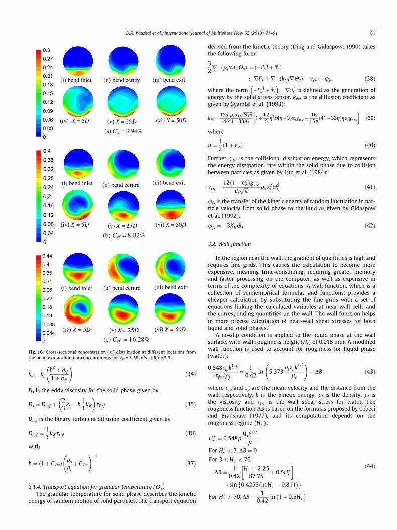
Fig. 16. Cross-sectional concentration (as) distribution at different locations fromthe bend exit at different concentrations for Vm = 3.56 m/s at R/r = 5.6.
D.R. Kaushal et al. / International Journal of Multiphase Flow 52 (2013) 71–91 81
ks ¼ kfb2 þ gsf
1þ gsf
!ð34Þ
Ds is the eddy viscosity for the solid phase given by
Ds ¼ Dt;sf þ23
ks � b13
ksf
� �sF;sf ð35Þ
Dt,sf is the binary turbulent diffusion coefficient given by
Dt;sf ¼13
ksf st;sf ð36Þ
with
b ¼ ð1þ CVmÞqs
qfþ CVm
!�1
ð37Þ
3.1.4. Transport equation for granular temperature (Hs)The granular temperature for solid phase describes the kinetic
energy of random motion of solid particles. The transport equation
derived from the kinetic theory (Ding and Gidaspow, 1990) takesthe following form:
32r � ðqsas~tsHsÞ ¼ ð�PsI þ ssÞ
: r~ts þr � ðkHsrHsÞ � cHs þufs ð38Þ
where the term �PsI þ ��ss
� �: rts! is defined as the generation of
energy by the solid stress tensor. kHs is the diffusion coefficient asgiven by Syamlal et al. (1993):
kHs¼15dsqsas
ffiffiffiffiffiffiffiffiffiffiHspp
4ð41�33gÞ 1þ125
g2ð4g�3Þasgo;ssþ16
15pð41�33gÞgasgo;ss
ð39Þ
where
g ¼ 12ð1þ essÞ ð40Þ
Further, cHsis the collisional dissipation energy, which represents
the energy dissipation rate within the solid phase due to collisionbetween particles as given by Lun et al. (1984):
cHs¼
12 1� e2ss
� �go;ss
dsffiffiffiffipp qsa
2s H
32s ð41Þ
ufs is the transfer of the kinetic energy of random fluctuation in par-ticle velocity from solid phase to the fluid as given by Gidaspowet al. (1992):
ufs ¼ �3KfsHs ð42Þ
3.2. Wall function
In the region near the wall, the gradient of quantities is high andrequires fine grids. This causes the calculation to become moreexpensive, meaning time-consuming, requiring greater memoryand faster processing on the computer, as well as expensive interms of the complexity of equations. A wall function, which is acollection of semiempirical formulas and functions, provides acheaper calculation by substituting the fine grids with a set ofequations linking the calculated variables at near-wall cells andthe corresponding quantities on the wall. The wall function helpsin more precise calculation of near-wall shear stresses for bothliquid and solid phases.
A no-slip condition is applied to the liquid phase at the wallsurface, with wall roughness height (Hs) of 0.015 mm. A modifiedwall function is used to account for roughness for liquid phase(water):
0:548tfpk1=2
sfw=qf¼ 1
0:42ln 5:373
qf zpk1=2
lf
!� DB ð43Þ
where tfp and zp are the mean velocity and the distance from thewall, respectively, k is the kinetic energy, qf is the density, lf isthe viscosity and sfw is the wall shear stress for water. Theroughness function DB is based on the formulas proposed by Cebeciand Bradshaw (1977), and its computation depends on theroughness regime Hþs
� �:
Hþs ¼ 0:548qHsk
1=2
lFor Hþs < 3;DB ¼ 0
For 3 < Hþs < 70
DB ¼ 10:42
Hþs � 2:2587:75
þ 0:5Hþs
� sin 0:4258 ln Hþs � 0:811
� �� �For Hþs > 70;DB ¼ 1
0:42ln 1þ 0:5Hþs� �
ð44Þ

(a) Water at bend inlet
(g) Sand at bend inlet
(b) Water at bend centre
(h) Sand atbend centre
(c) Water at bend exit
(i) Sand at bend exit
(d) Water at X = 5D
(j) Sand at X = 5D
(e) Water at X = 25D
(k) Sand at X = 25D
(f) Water at X = 50D
(l) Sand at X = 50D
Fig. 17. Distributions of tfz and tsz in m/s at Cvf = 8.82% and Vm = 3.56 m/s.
(a) Water (b) Sand
Fig. 18. Contours of magnitude and directions of velocity component in the plane perpendicular to the direction of flow in m/s for Cvf = 8.82% and Vm = 3.56 m/s at bendcentre.
82 D.R. Kaushal et al. / International Journal of Multiphase Flow 52 (2013) 71–91
In the FLUENT (2006) solver, DB is evaluated using thecorresponding formula in Eq. (44). The modified law of the wallin Eq. (43) is then used to evaluate the shear stress at the walland other wall functions for the turbulent quantities for water.
For solid phase (silica sand), the semi-empirical equationsdeveloped by Johnson and Jackson (1987), expressed as Eqs. (45)and (46) are used to calculate the solid tangential velocity andgranular temperature at wall. Specularity coefficient /w representsthe tangential momentum loss in the particle–wall collisions, andhigh granular energy will be produced at the high specularitycoefficient. The investigations of slurry flows show that it isdifficult to measure the specularity coefficient /w and the parti-
cle–wall restitution coefficient ew in the experiment, so the appro-priate values for a specified flow system are generally determinedby sensitivity analysis in the numerical investigations (Benyahiaet al., 2007).
~ts;w ¼ �6lsas;maxffiffiffi
3p
p/wqsgo;ss
ffiffiffiffiffiffiffiffiffiffiHs;w
p @~ts;w
@nð45Þ
Hs;w ¼ �jHs;w
cw
@Hs;w
@nþ
ffiffiffi3p
p/wqsas~t2s;wgo;ssH
3=2s;w
6as;maxcwð46Þ
where cw ¼ffiffi3p
p 1�e2wð Þasqsgo;ssH
3=2s;w
4as;max.

(a) Water (b) Sand
Fig. 19. Contours of magnitude and directions of velocity component in the plane perpendicular to the direction of flow in m/s for Cvf = 8.82% and Vm = 3.56 m/s at bend exit.
D.R. Kaushal et al. / International Journal of Multiphase Flow 52 (2013) 71–91 83
The parameters used in the model are determined referring tothe previous numerical and experimental studies on slurry flowswith the same type of particles. The particle–wall restitutioncoefficient ew is taken as 0.99 and the specularity coefficient
(a) Water
Fig. 20. Contours of magnitude and directions of velocity component in the plane perpe
/w used in the Johnson–Jackson wall boundary conditions is0.0001, namely only 0.01% of tangential momentum is lost afterthe particle–wall collisions (Benyahia et al., 2007; Pain et al.,2001).
(b) Sand
ndicular to the direction of flow in m/s for Cvf = 8.82% and Vm = 3.56 m/s at X = 5D.

(a) Water at bend centre
(d) Sand at bend centre
(b) Water at bend exit
(e) Sand at bend exit
(c) Water at X = 5D
(f) Sand at X = 5D
Fig. 21. Contours of magnitude and directions of vertical velocities tfz(x, y) and tsz(x, y) in m/s for Cvf = 8.82% and Vm = 3.56 m/s.
84 D.R. Kaushal et al. / International Journal of Multiphase Flow 52 (2013) 71–91
Centrifugal force due to presence of bend gets calculated auto-matically by FLUENT based on the development of radial pressuregradient due to curved streamlines along the bend section.
4. Numerical solution
4.1. Geometry
In single phase flow it is well established that an entrancelength of 30D to 50D is necessary to establish fully developedturbulent pipe flow. Whilst such estimates were used as a guide,a series of numerical trials were conducted using different pipelengths. For all of the cases simulated here, a pipe length of 32D
was sufficient to give a fully developed slurry flow at the upstreamof bend inlet. Using a longer pipe did not affect the results. In viewof this, the reference pressure is chosen 32D upstream of the bendinlet. As the present study is focussed on analyzing the slurry-flowbehavior in 90� horizontal bend only, there is no use of taking ref-erence point at distance larger than 32D. Velocity inlet is kept15 cm upstream of reference point which is at 32D upstream ofthe bend inlet (Fig. 2). The bend is laid horizontally in (x, y) planewith origin (0, 0, 0) at centre of velocity inlet. The direction of flowat velocity inlet is in positive-y direction. The direction of flow atpressure outlet is in negative-x direction. The mid-vertical planeis in the z-axis intersecting pipe cross-section at the centre. Themid-horizontal plane is along the x and y-axis in (x, y) plane at

(a) Bend centre (b) Bend exit (c) X = 5D
Fig. 22. Contours of slip velocity (tsz � tfz) in the plane perpendicular to the direction of flow in m/s for Cvf = 8.82% and Vm = 3.56 m/s.
0
0.2
0.4
0.6
0.8
1
z'
Predicted
Experimental
0
0.2
0.4
0.6
0.8
1z'
Predicted
Experimental
0 1 2 3 4 5 6 7
Normalised Concentration
(a) X = 5D
0 1 2 3 4 5 6 7
Normalised Concentration
(b) X =25 D
0
0.2
0.4
0.6
0.8
1
0 1 2 3 4 5 6 7
z'
(c) X = 50DNormalised Concentration
Predicted
Experimental
Fig. 23. Comparison between measured and predicted mid-vertical concentration profiles at different locations in the downstream of bend exit at Cvf = 3.94% andVm = 1.78 m/s (Normalized concentration = as(z0)/Cvf).
D.R. Kaushal et al. / International Journal of Multiphase Flow 52 (2013) 71–91 85
velocity inlet and pressure outlet, respectively, intersecting pipecross-section at the centre.
The computational grid for the bend similar to that used in exper-iments consisting of 266,670 cells and 303,456 nodes (Figs. 2 and 3)
has been generated using GAMBIT software. This number was gener-ated by applying the same cross-sectional meshes obtained from theoptimum cross-sectional meshes of pipe for the single-phase flow.The grid-independence tests were carried out keeping all the solver
0.2
0.4
0.6
0.8
1
z'
Predicted
Experimental
0.2
0.4
0.6
0.8
1
z'
Predicted
Experimental
00 1 2 3 4
Normalised Concentration
(a) X = 5D
00 1 2 3 4
Normalised Concentration
(b) X = 25D
0
0.2
0.4
0.6
0.8
1
0 1 2 3 4
z'
Normalised Concentration
(c) X = 50D
Predicted
Experimental
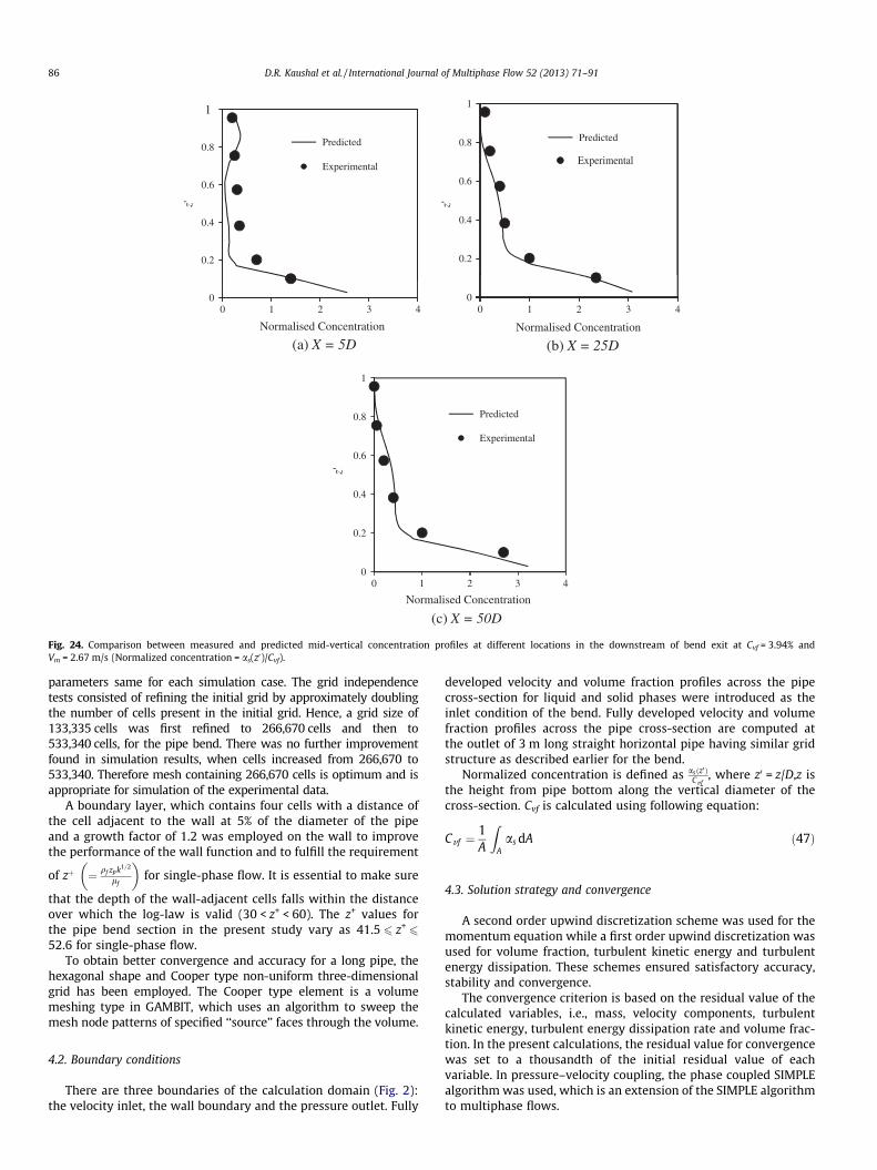
Fig. 24. Comparison between measured and predicted mid-vertical concentration profiles at different locations in the downstream of bend exit at Cvf = 3.94% andVm = 2.67 m/s (Normalized concentration = as(z0)/Cvf).
86 D.R. Kaushal et al. / International Journal of Multiphase Flow 52 (2013) 71–91
parameters same for each simulation case. The grid independencetests consisted of refining the initial grid by approximately doublingthe number of cells present in the initial grid. Hence, a grid size of133,335 cells was first refined to 266,670 cells and then to533,340 cells, for the pipe bend. There was no further improvementfound in simulation results, when cells increased from 266,670 to533,340. Therefore mesh containing 266,670 cells is optimum and isappropriate for simulation of the experimental data.
A boundary layer, which contains four cells with a distance ofthe cell adjacent to the wall at 5% of the diameter of the pipeand a growth factor of 1.2 was employed on the wall to improvethe performance of the wall function and to fulfill the requirement
of zþ ¼ qf zpk1=2
lf
� �for single-phase flow. It is essential to make sure
that the depth of the wall-adjacent cells falls within the distanceover which the log-law is valid (30 < z+ < 60). The z+ values forthe pipe bend section in the present study vary as 41.5 6 z+
6
52.6 for single-phase flow.To obtain better convergence and accuracy for a long pipe, the
hexagonal shape and Cooper type non-uniform three-dimensionalgrid has been employed. The Cooper type element is a volumemeshing type in GAMBIT, which uses an algorithm to sweep themesh node patterns of specified ‘‘source’’ faces through the volume.
4.2. Boundary conditions
There are three boundaries of the calculation domain (Fig. 2):the velocity inlet, the wall boundary and the pressure outlet. Fully
developed velocity and volume fraction profiles across the pipecross-section for liquid and solid phases were introduced as theinlet condition of the bend. Fully developed velocity and volumefraction profiles across the pipe cross-section are computed atthe outlet of 3 m long straight horizontal pipe having similar gridstructure as described earlier for the bend.
Normalized concentration is defined as asðz0 ÞCvf
, where z0 = z/D,z isthe height from pipe bottom along the vertical diameter of thecross-section. Cvf is calculated using following equation:
Cvf ¼1A
ZAas dA ð47Þ
4.3. Solution strategy and convergence
A second order upwind discretization scheme was used for themomentum equation while a first order upwind discretization wasused for volume fraction, turbulent kinetic energy and turbulentenergy dissipation. These schemes ensured satisfactory accuracy,stability and convergence.
The convergence criterion is based on the residual value of thecalculated variables, i.e., mass, velocity components, turbulentkinetic energy, turbulent energy dissipation rate and volume frac-tion. In the present calculations, the residual value for convergencewas set to a thousandth of the initial residual value of eachvariable. In pressure–velocity coupling, the phase coupled SIMPLEalgorithm was used, which is an extension of the SIMPLE algorithmto multiphase flows.

0
0.2
0.4
0.6
0.8
1
z'
Predicted
Experimental
0
0.2
0.4
0.6
0.8
1
z'
Predicted
Experimental
00 1 2 3 4
Normelised Concentration
(a) X = 5D
00 1 2 3 4
Normalised Concentration
(b) X =25D
0
0.2
0.4
0.6
0.8
1
0 1 2 3 4
z'
Normalised Concentration
(c) X = 50D
Predicted
Experimental
Fig. 25. Comparison between measured and predicted mid-vertical concentration profiles at different locations in the downstream of bend exit at Cvf = 3.94% andVm = 3.56 m/s (Normalized concentration = as(z0)/Cvf).
D.R. Kaushal et al. / International Journal of Multiphase Flow 52 (2013) 71–91 87
Parametric analysis was undertaken to assess the sensitivityof simulation results to various input parameters and todetermine appropriate default parameters and methodologiesfor predicting the different properties of slurry flow throughpipeline.
5. Modeling results
5.1. Pressure drop for single-phase flow at different radius ratios
The pressure drops are presented in the normalized form½¼ Dp=ðqwV2
m=2Þ, where, Dp is the pressure drop with referenceto 32D upstream of bend inlet, qw is the density of water and Vm
is the mean flow velocity calculated by dividing the measured dis-charge by pipe cross-sectional area. Normalized pressure dropshave been evaluated for simulated geometry for seven pipe bendsat five mean flow velocities from 0.89, 1.34, 1.78, 2.67, up to3.56 m/s. The corresponding range of Reynolds number is(0.64 � 105–2.50 � 105). Pressure drop distributions obtained byexperiments and CFD modeling for flow of water are presentedin Fig. 4 for R/r = 5.60 at the flow velocity of 3.56 m/s. As expected,the pressure decreases along the flow constantly before the bend.However, as the flow reaches near the bend, the pressure decreasesrapidly in comparison to the straight section. Figs. 5 and 6 showthe pressure changes across the horizontal bend cross-section.The increased pressure at the outer wall of the bend is due to vor-tex formation.
The total bend loss coefficient (kt) is defined as
kt ¼Dpt
qwV2m
2
� � ð48Þ
where Dpt is the bend pressure drop.The measured and simulated bend loss coefficients (kt) are
evaluated for each run and drawn graphically in Fig. 7. It is alsoobserved that values of kt reduce from a highest value for theelbow having radius ratio 0.0 to the lowest value for the radiusratio 5.60 and increase thereafter, a feature observed at all flowrates. The high pressure loss in a sharp elbow can be attributedto the generation of strong secondary flows due to the sharp turn.It is observed that the CFD modeling gives fairly accurate predic-tions (with percentage error in the range of ±10%) for kt at all flowvelocities considered in the present study. In the present case, R/D > 1,2 � 104 < Re < 4 � 105, Ito (1960) gave following correlationfor kt:
kt ¼0:3897f0:95þ 4:42=ðR=DÞ1:96gðR=DÞ0:84
R0:17e
; Re=ðR=DÞ2 > 364
ð49Þ
where Re ¼ VmDm ; m is kinematic viscosity of water.
It is observed that both the measured and CFD predictions forrough bends used in the present experiment are larger than thevalues predicted by Ito (1960) for smooth bends as shown inFig. 8. Such a difference is obvious due to roughness of pipe bends.

0
0.2
0.4
0.6
0.8
1
z'
Predicted
Experimental
0
0.2
0.4
0.6
0.8
1
z'
Predicted
Experimental
0 1 2 3 4 5
Normalised Concentration
(b) X = 25D
0 1 2 3 4 5
Normalised Concentration
(a) X = 5D
0
0.2
0.4
0.6
0.8
1
0 1 2 3 4 5
z'
Normalised Concentration
(c) X = 50D
Predicted
Experimental
Fig. 26. Comparison between measured and predicted mid-vertical concentration profiles at different locations in the downstream of bend exit at Cvf = 8.82% andVm = 1.78 m/s (Normalized concentration = as(z0)/Cvf).
88 D.R. Kaushal et al. / International Journal of Multiphase Flow 52 (2013) 71–91
However, CFD predictions are well in line with Ito (1960) correla-tion for smooth bends and experimental data for rough bends asshown in Fig. 8.
5.2. Pressure drop for slurry flow in bend having R/r of 5.60
The pressure drops in mid-horizontal plane are presented inFig. 9 in the normalized form as Dp=ðqmV2
m=2Þ, where Dp is thepressure drop with reference to the 32D upstream of bend inletat a particular point, qm is the measured density of slurry, Vm isthe mean flow velocity calculated by dividing the measured dis-charge by pipe cross-sectional area for efflux concentration of3.94–16.28% at flow velocities of 1.78 and 3.56 m/s.
Comparison between measured and predicted normalized pres-sure drops is shown in Figs. 10–12. From these figures, it is clearlyseen that the CFD can predict the pressure drop with fair accuracyfor slurry flow through horizontal 90 degree bend. However, as theefflux concentration increases, the CFD results begin to deviatefrom the measured values. The deviation increases with the con-centration. It is observed that the CFD modeling gives predictionswith percentage error in the range of ±10% for pressure drop atall flow velocities considered in the present study.
The measured and predicted bend loss coefficients (kt) aredrawn graphically in Fig. 13. It is observed that kt reduces with in-crease in flow velocity, and decrease in efflux concentration. It isobserved that the CFD modeling gives fairly accurate predictions(with percentage error in the range of ±10% except few data at
higher concentration) for kt at all flow velocities considered inthe present study.
5.3. Concentration distribution at bend
Cross-sectional concentration distributions (as) as predicted byCFD at six different locations (namely, bend inlet, bend centre,bend exit, X = 5D, 25D and 50D, where X is the distance from bendexit) for efflux concentration 3.94%, 8.82% and 16.28% at flowvelocities 1.78 m/s, 2.67 m/s and 3.56 m/s are shown in Figs. 14–16. In these figures, left hand side represents the outer wall,whereas right hand side represents inner wall of the bend. The con-centration distributions are skewed towards the bottom and thisskewness being higher for lower velocity of 1.78 m/s. At highervelocities of 2.67 m/s and 3.56 m/s, the concentration distributionis more uniform. At bend centre, bend exit and X = 5D, the particlesare forced outwards due to the secondary flow. This secondary flowinfluences the motion of particles even after the bend and theincreased concentrations at the outer wall of bend can be clearlyseen at these locations for all the concentrations and flow veloci-ties (Figs. 14–16). This effect is maximum at X = 5D resulting intoa central zone of very low concentration at the centre of pipeline.It is observed that in upstream side of bend inlet, X = 25D andX = 50D, flow behavior is almost similar to the flow in straightsection. The concentration profile becomes more uniformdownstream of bend exit. This effect is more visible with increas-ing flow velocity as the increased strength of turbulent eddies

0
0.2
0.4
0.6
0.8
1
z'
Predicted
Experimental
0
0.2
0.4
0.6
0.8
1
z'
Predicted
Experimental
0 1 2 3 4
Normalised Concentration
(a) X = 5D
00 1 2 3 4
Normalised Concentration
(b) X = 25D
0
0.2
0.4
0.6
0.8
1
0 1 2 3 4
z'
Normalised Concentration
(c) X = 50D
Predicted
Experimental
Fig. 27. Comparison between measured and predicted mid-vertical concentration profiles at different locations in the downstream of bend exit at Cvf = 8.82% andVm = 2.67 m/s (Normalized concentration = as(z0)/Cvf).
D.R. Kaushal et al. / International Journal of Multiphase Flow 52 (2013) 71–91 89
formed due to the change in flow direction. However, at the bendinlet, the concentration profile does not deviate much from that inthe upstream side.
In Fig. 17, distributions of tfz and tsz in m/s at Cvf = 8.82% andVm = 3.56 m/s are shown. Deformation in velocity profiles due tothe presence of bend is more prominent at bend centre, bend exitand X = 5D. Zone of higher velocity is shifted away from centre atthese locations. Such deformation in velocity profile may be attrib-uted to the secondary flow. However, at bend inlet, bend exit andX = 5D, zone of higher velocity remains in the central core of pipecross-secton.
Figs. 18–20 show the contours of magnitude and directions ofvelocity component in the plane perpendicular to the flow direc-tion in m/s for Cvf = 8.82% and Vm = 3.56 m/s at bend centre, bendexit and X = 5D, respectively. Secondary flow begins to develop atbend centre (Fig. 18), it is fully developed at bend exit (Fig. 19)and remains developed at X = 5D (Fig. 20). However, the velocitycomponents in the plane perpendicular to the flow direction atbend inlet, X = 25D and X = 50D are negligible (0–0.1 m/s forVm = 3.56 m/s) due to the absence of secondary flows at theselocations.
The observations made previously from Figs. 14–20 are reaf-firmed in Fig. 21 showing the z-component of velocity for waterand sand. High values at bend centre, bend exit and X = 5D reflectsstrong effect of secondary flows. This effect creates zones of posi-tive and negative values at left (outer wall of bend) and right (innerwall of bend) corner in the upper half of pipeline, respectively.
Positive zone situated at outer wall of bend is more prominent atbend centre due to free passage for water and sand particles (Figs.21a and d and 16b). The diminishing of positive zone at X = 5D maybe attributed to the movement of sand particles into the positivezone situated at the outer wall of bend hindering the movementof more water and sand particles due to gravitational effects (Figs.21c and f and 16b). Negative zone situated at the inner wall of bendis more prominent at X = 5D as the gravitational effect and the pres-ence of sand particles enhances the downward movement of waterand sand particles (Figs. 21c and f and 16b). Negative zone situatedat inner wall at bend centre is not prominent due to absence of sandparticles (Figs. 21a and d and 16b). Very low values of tfz(x, y) andtsz(x, y) at bend inlet, X = 25D and X = 50D reflect diminishing effectdue to the secondary flows are not shown in this figure.
Fig. 22 shows the contours of z component of slip velocity (dif-ference in z components of velocity for sand and water) in theplane perpendicular to the direction of flow in m/s for Cvf = 8.82%and Vm = 3.56 m/s. At bend centre, velocity component of sand ismore than that of water, forcing sand particles towards outer wallof bend (Fig. 16b). These particles are trapped in secondary flowsand move further up along the pipe wall. The positive slip velocityin the outer periphery as shown in Fig. 22b and c at bend exit andX = 5D keeps more particles moving in the outer ring near pipewall.
Particles segregate in a small portion of the pipe cross-sectionclose to the outer wall in bend due to the action of centrifugalforces. These particles impinging on the outer wall, form a

0
0.2
0.4
0.6
0.8
1
z'
Predicted
Experimental
0
0.2
0.4
0.6
0.8
1
z'
Predicted
Experimental
0 1 2 3 4
Normalised Concentration
(a) X = 5D
0 1 2 3 4
Normalised Concentration
(b) X = 25D
0
0.2
0.4
0.6
0.8
1
0 1 2 3 4
z'
Normalised Concentration
(c) X = 50D
Predicted
Experimental
Fig. 28. Comparison between measured and predicted mid-vertical concentration profiles at different locations in the downstream of bend exit at Cvf = 8.82% andVm = 3.56 m/s (Normalized concentration = as(z0)/Cvf).
90 D.R. Kaushal et al. / International Journal of Multiphase Flow 52 (2013) 71–91
relatively dense phase structure in a small portion of the pipecross-section close to the outer wall that is termed as rope(concentration distributions at bend centre and bend exit shownin Figs. 14–16). Just after the bend, transport of particles ismainly due to the roping effect. The region of the rope has amuch higher solid concentration than the remainder of the pipe.This high concentration increases the particle–particle collisionsand causes the particles to decelerate. In other words, increasedsolids pressure results into the decrease in momentum of theparticles (velocity distributions at bend centre, bend exit andX = 5D shown in Figs. 18–21). The ropes were dispersed furtherdown the bend where the particles accelerate and a secondaryflow carries them around the pipe circumference and eventuallyto the middle of the pipe where turbulence causes them tospread over the entire cross-section (concentration distributionsat X = 5D in Figs. 14–16).
An overall review based on the above discussion for the concen-tration distribution of mono-dispersed slurry at different locationsin the bend having radius ratio 5.60 reveals the following:
a. The re-distribution of solid particles takes place downstreamof the bend due to the secondary flows. This effect is seenclose to the bend and decays with increase in distance.
b. The concentration distribution is more uniform just down-stream of the bend. The skewness in the concentration pro-file increases with downstream distance from the bend exit.
c. At the bend inlet, the concentration profile does not deviatemuch from that in the upstream side.
In the present study, as is measured at X = 5D, 25D and 50Dfrom bend exit using sampling tubes C1, C2 and C3 (Fig. 2) atz0 = 0.094, 0.189, 0.377, 0.566, 0.755 and 0.943. Figs. 23–28 pres-ent the measured and predicted normalized solids concentrationprofiles using CFD in mid-vertical plane in downstream side ofbend for flow velocities of 1.78, 2.67 and 3.56 m/s at solidconcentrations of 3.94% and 8.82%. In the present study, the con-centration profiles measured at the same plane are used forcomparison. The swirling flow due to secondary flow at bendmakes the concentration at the top of pipe higher than that incentral core near the bend exit at X = 5D. Figs. 23–28 exhibit rea-sonably good agreement between experimental and modelingvalues except for few cases.
6. Conclusions
The ability of implemented Eulerian model in FLUENT softwareto predict the pressure drop and concentration profile across a 90�horizontal pipe bend in slurry pipeline transporting silica sandusing standard input parameters was investigated. Overall, therewas broad qualitative and quantitative agreement in trends andflow patterns. The results suggest that the Eulerian model is rea-
D.R. Kaushal et al. / International Journal of Multiphase Flow 52 (2013) 71–91 91
sonably effective with the slurry pipe bend in the horizontal plane.We examine the possibility of FLUENT software when it is appliedto slurry flow in a bend. In this software, k–e model is used to ob-tain fluid Reynolds stresses and the kinetic theory model is used toobtain solid phase stresses like fluid molecular stresses. Theseequations are solved coupling with other equations. We couldget many interesting results by this approach, which are compara-ble to the measurements.
Followings are the specific conclusions based on the presentstudy:
i. Measured and predicted normalized pressure drop and bendloss coefficient show good agreement for flow of water in awide range of R/r values from 0 to 5.89, with a maximum±10% difference.
ii. CFD modeling gives fairly accurate pressure drops (withinpercentage error of ±10% except few data at higher concen-tration) for the flow of silica sand slurry having particlediameter of 450 lm in the efflux concentration from 0% to16.28% at different flow velocities from 1.78 to 3.56 m/s.
iii. Velocity and concentration distributions of solids get almostuniform shortly after the bend.
iv. The redistribution of solid particles takes place downstreamof the bend due to the secondary flows. This effect is seenclose to the bend exit, and with increase in distance thiseffect decays in the mid-vertical plane.
References
Benyahia, S., Syamlal, M., O’Brien, T.J., 2007. Study of the ability of multiphasecontinuum models to predict core-annulus flow. AIChE J. 53, 2549–2568.
Cebeci, T., Bradshaw, P., 1977. Momentum Transfer in Boundary Layers. HemispherePublishing Corporation, New York.
Ding, J., Gidaspow, D., 1990. A bubbling fluidization model using kinetic theory ofgranular flow. AIChE J. 36, 523–538.
Drew, D.A., Lahey, R.T., 1993. Particulate Two – Phase Flow. Butterworth-Heinemann Publications, Boston, pp. 509–566.
FLUENT, 2006. User’s Guide Fluent 6.2. Fluent Incorporation, USA.Garside, J., Al-Dibouni, M.R., 1977. Velocity-voidage relationships for fluidization
and sedimentation. I & EC Process Des. Dev. 16, 206–214.
Gidaspow, D., Bezburuah, R., Ding, J., 1992. Hydrodynamics of circulating fluidizedbeds, kinetic theory approach in fluidization VII. In: Proceedings of the 7thEngineering Foundation Conference on Fluidization.
Ito, H., 1960. Pressure losses in smooth pipe bends. J. Basic Eng. ASME 82D,131–143.
Johnson, P., Jackson, R., 1987. Frictional–collisional constitutive relations forgranular materials, with application to plane shearing. J. Fluid Mech. 176,67–93.
Kalyanraman, K., Ghosh, D.P., Rao, A.J., 1973. Characteristics of sand water slurry in90� horizontal pipe bend. Inst. Eng. (India) J. 54, 73–79.
Kaushal, D.R., Tomita, Y., 2002. Solids concentration profiles and pressure drop inpipeline flow of multisized particulate slurries. Int. J. Multiphase Flow 28,1697–1717.
Kumar, A., 2010. Experimental and CFD Modeling of Hydraulic and PneumaticConveying through Pipeline. Ph.D. Thesis. I.I.T. Delhi.
Kumar, A., Kaushal, D.R., Kumar, U., 2008. Bend pressure drop experimentscompared with FLUENT. Inst. Civil Eng. J. Eng. Comput. Mech. 161, 35–45.
Launder, B.E., Spalding, D.B., 1974. The numerical computation of turbulent flows.Comput. Meth. Appl. Mech. Eng. 3, 269–289.
Ling, J., Skudarnov, P.V., Lin, C.X., Ebadian, M.A., 2003. Numerical investigations ofliquid–solid slurry flows in a fully developed turbulent flow region. Int. J. HeatFluid Flow 24, 389–398.
Lun, C.K.K., Savage, S.B., Jeffrey, D.J., Chepurniy, N., 1984. Kinetic theories forgranular flow: inelastic particles in couette flow and slightly inelastic particlesin a general flow field. J. Fluid Mech. 140, 223–256.
Pain, C.C., Mansoorzadeh, S., de Oliveira, C.R.E., 2001. A study of bubbling andslugging fluidised beds using the two-fluid granular temperature model. Int. J.Multiphase Flow 27, 527–551.
Richardson, J.R., Zaki, W.N., 1954. Sedimentation and fluidization: Part I. Trans. Inst.Chem. Eng. 32, 35–53.
Schaan, J., Sumner, R.J., Gillies, R.G., Shook, C.A., 2000. The effect of particle shape onpipeline friction for Newtonian slurries of fine particles. Can. J. Chem. Eng. 78,717–725.
Schaeffer, D.G., 1987. Instability in the evolution equations describingincompressible granular flow. J. Diff. Eq. 66, 19–50.
Syamlal, M., Rogers, W., O’Brien, T.J., 1993. MFIX Documentation. Theory Guide, vol.1. National Technical Information Service, Springfield, VA.
Thinglas, T., Kaushal, D.R., 2008a. Comparison of two dimensional and threedimensional CFD modeling of invert trap configuration to be used in sewer solidmanagement. Particuology 6, 176–184.
Thinglas, T., Kaushal, D.R., 2008b. Three dimensional CFD modeling for optimizationof invert trap configuration to be used in sewer solid management. ParticulateSci. Technol. 26, 507–519.
Toda, M., Kamori, N., Saito, S., Maeda, S., 1972. Hydraulic conveying of solidsthrough pipe bends. J. Chem. Eng. Jpn. 5, 4–13.
Turian, R.M., Ma, T.W., Hsu, F.L., Sung, D.J., Plackmann, G.W., 1998. Flowof concentrated non-Newtonian slurries: 2. Friction losses for flow inbends, fittings, valves and Venturi meters. Int. J. Multiphase Flow 24,243–269.