INCREASE OF EXCHANGEABLE CARBON IN THE EARTH'S RESERVOIRS

FROM COMBUSTION OF FOSSIL FUELS

Doris J. Dugas

December 1968

IID1~r

INCREASE OF EXCHANGEABLE CARBON IN THE EARIT'S RESERVOIRSFROM COMBUSTION OF FOSSIL FJELS

Doris J Dugas

The RAND Corporation, Santa Monica, California

ABSTRACT

The distribution of excess carbon dioxide produced during and after

the consumption of all fossil fuel is determined with the aid of a foir-

reservoir moi-i of carbon exchange as developed previoti"ly for carbon-

14. From estimates of the total hydrocarbon fuel resources originally

on earth. it is calculated that about 3000 billion tons of carbon ulti-

mately may be released to the atmosphere from this source, At a moder-

ate consumption rate, this fuel supply will be consumed within 200 years

and, according to the model, the atmospheric carbon dioxide concentra-

tion will reach a maximum value of twice its normal (pre-1900) concen-

tration before declining to a new equilibriur level about 8 percent

above the normal. Carbon excess in the surface layers of the ocean

reaches a peak a few years later than the ;tmosphere and retains some-

what less of the excess carbon at equilibrium, while the deep sea even-

tually absorbs over 90 percent of the excess carbon released by fossil

fuel consumption. It was fount that the results are highly sensitive

to the assumptions as to future fossil fuel consumption rates, but that

the atmospheric carbon concentration is not critically affected by the

amount of direct exchange between the atmosphere and deep sea.

Any views expressed in this paper are those of the author. Theyshould not be interpreted as reflecting the views of The RAND Corpora-tion or the official opinion or policy of any ( its governmental orprivaLe research sponsors. Papers are reproduct bv The RAND Corpora-tion as a courtesy to members of its staff.

This paper was prepired Ior pub li.at ion in Jouril I i f Geophysi calResearch.

-2-

INTRODUCTION

Carbon dioxide is the only one of the m3ny air pollutan s that

has been identified as increasing on a global scale. Measuterments in

recent years have shown that the carbon dioxide concentration in the

atmosphere has been slowly increasing since the late 19th century

[Callendar, 1958] and the current annual rate ,)f increase appears to

be about 0.7 parts per million (ppm) measured over the oceans [Bolin

and Keeling, Q61], Local and temporal variations nay be much greater

than this according to temperature, amount of vegetation, season, in-

dustrial activity, and volcanism. The general increase has often been

attributed to human activities involving the combustion of ever larger

quantities of hydrocarbon fuels; consequently the prospect of gradual

industrialization over most of the earth evokes predictions of huge

carbon dioxide concentrations in the atmosphere. However, cab5on di-

oxide released to the atmosphere is continually being mix :d with other

reservoirs--the oceans, soil, biosphere--and the oceans, being the

largest reservoir for carbon dioxide, are especially important in with-

drawing excess carbon from the atmospherc

In view of the possibility of long term Llimatic changes due to

variations in carbon dioxide concentration in the atmosphere, it is

of particular interest to determine tow great such variations may be-

come. An upper limit may be calculated by assuming that mait will con-

sume the total supply of fossil fuels remaining in the earth. This

paper will be concerned with the quantitative exchange of carbon be-

tween the earth's natural reservoirs, ind particularly with the rate

at which an excess of carbon dioxide in the atniosphere caused by

I -

-3-

combc-ttion products Aill decay with time. To do this, the tour-reservoir

moide] 4,, exchange and the exchange rate constants established from radio-

carbo;:, ditn wvill. be used! [les.user and Dugab, 1966].

-4-

FOSSI FUEL RESOURCES

StatisLics on the amount of fossil fuel (that is, el derived

from geologic deposits of organic matter, including coal, netroleum

and gas) thus far produced on earth are given in Table I. Data prior

to 1961 were obtained from Hubbert (1962) and statistics for recent

years were gathered from the world production tables published by the

Bureau of Mines (1963-1966).

Numerous estimates of the amount of fossil fuel remaining in the

earth have been made. There are wide discrepanices between estimates,

with the later ooes generally being larger than earlier ones, reflect-ing more thorough geological surveys, imprLved recovery methods andI;

more oxperienc, with proven reserves. Recent figures from the U.S.

Geological Survey [Averitt, 1968 and Hendricks, 1965] for the petroleum

and natural gas resources remaining in place in the world are also

given in Table I. The estimates were obtained by classifying sedimen-

tary basins of the world, including the continental shelves, then ap-

plying known productivity factors of similar U.S. basins. ',te that

"ton" as used throughout this paper refers to the metric ton (1000 kg

rr ?2O0 Ib) Whe. original data were given in b..rrels, they have been

converted here to metric tors assuming an average specific gravity for

crude oil and natural gas liquids of 0.92.

World coal resources wevc not included in U.S.G.S. estimates, so

a prior L.timate ot Weeks 19601 is given in the table. It includes

all grades of antoracite, bituminous, and lignite, even though they

may he in narrow seams or deep deposits that art, not now commercially

exp)loitable Some large claims for coal resources in USSR and China

-5-

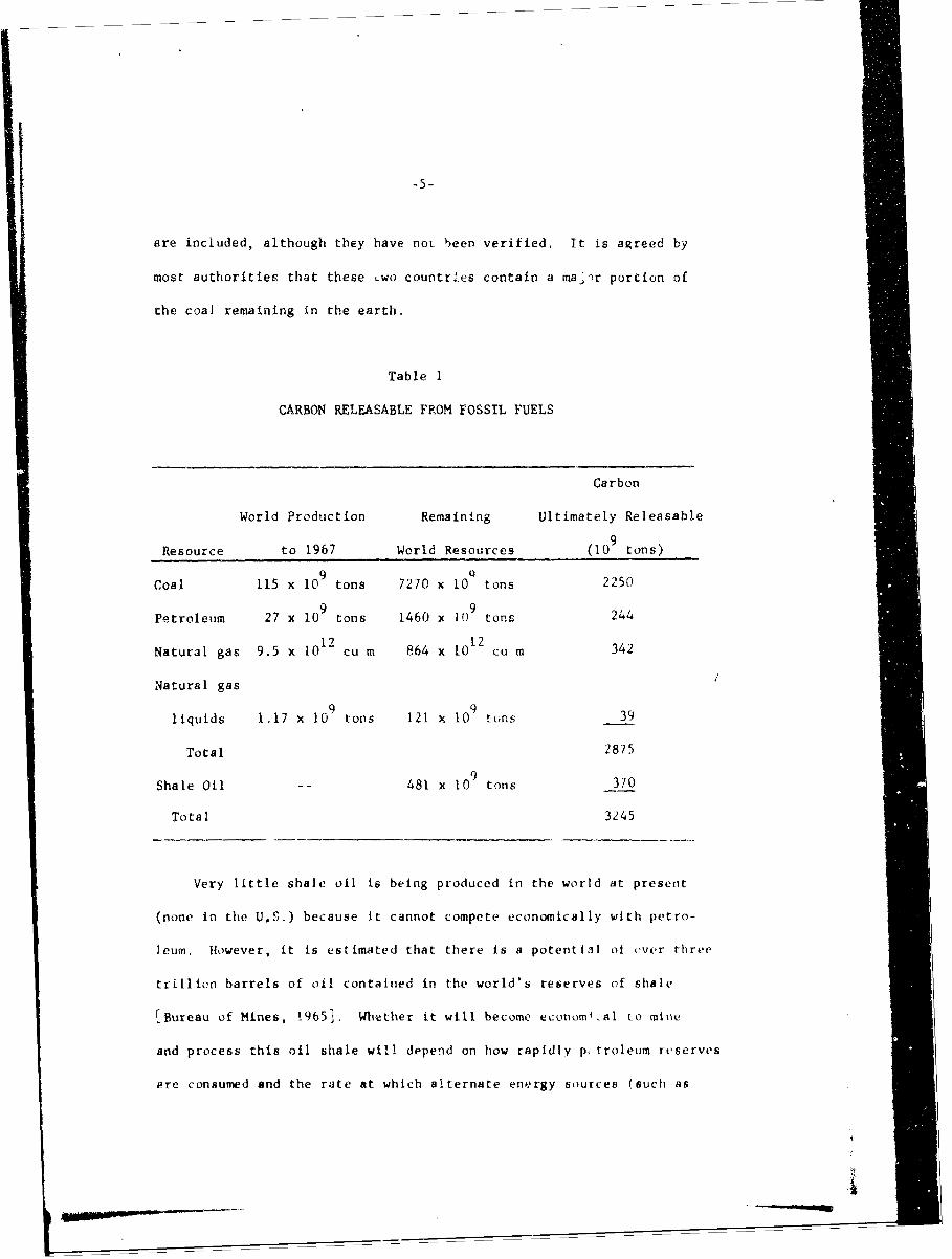
are included, although they have not been verified. It is agreed by

most authorities that these Lwo countries contain a ma,-r porcion of

the coal remaining in the earth.

Table 1

CARBON RELEASABLE FROM FOSSIL FUELS

Carbon

World Production Remaining Ultimately Releasable

Resource to 1967 World Resources (109 tons)

Coal 115 x 109 tons 7270 x 10 tons 2250

Petroleum 27 x 109 tons 1460 x 109 ton- 244

112 012Natural gas 9.5 x 10 cu m 864 x 10 cu m 342

Natural gas

liquids 1.17 x 109 tons 121 x 109 tons 39

Total 2875

Shale Oil 481 x 109 tons 370

Total 3245

Very little shale oil is being produced in the world at present

(none in the U.S.) because it cannot compete economically with petro-

leum. However, it is estimated that there is a potential of over three

trillion barrels of oil contained in the world's reserves of shale

[Bureau of Mines, 19651. Whether it will become economical to mine

and process this oil shale will depend on how rapidly p troleum reserves

ore consumed and the rate at which alternate energy sources (such as

nuclear) are expanded. Since the future of the shale oil industry Is

still fairiy uncertain, two values for the total carbon ultimately re-

leaseable have been determined: one assumes all shale oil reserves

will be consumed, and one that disregards shale oil altogether.

In o.-der to add the fuel resources listed in Table 1, each has

been reduced to the common base of tons of carbon ultinately release-

able. This conversion involved the expected recovery rate for each

resource originally in place, and the average carbon content of the

recovered fuel. The factors which were used in this conversion are

listed in Table 2. They arp, of course, subject to revision as tech-

nology progresses and demand changes, It is presumed that all (if the

carDon in a fuel as produced will eventually be oxidized and reach the

atmosphere as carbon dioxide, even though it may be wasted, tempor-

arily stored, or inefficiently consumed.

Table 2

RECOVERY RATE AND CARBON CONTENT OF

HYDROCARBON FUEL RESOURCES

Fraction of Average

Resource Carbon

Resource Recoverable Content (v)

Coal

Petroleum b4

Natural gas 78

Natural gas liquids 64

Shale oil all 77

Resource is estimated in terms of recover-

ahle oil r-ther than oitl in plate.

-7-

Adding the releasable carbon for fuel already consumed and remain-

ing resources gives the total for a,I time of 2875 billion tons (or

3245 billion tons if shale oil is included). ThiLs represents 4.9 times

(or 5.5 times) the amount of carbon in the atmosphere before 1900.

-8-

CARBON EXCHANGE MODEL

After the method previously developed [Plesset and Dugas, 1966],

four reservoirs of carbon dioxide will be considered to exchange as

indicated schematically in Fig. I. The equations for exchange of car-

bon among the four reservoirs under equilibrium conditions (that is,

before significant hydrocarbon fuel consump:ion begins) are:

-KadNa K amNa - KahMa KdaNd MaNm+KhaNh 0 (1)

-KhaNh + Kh a N 0 (2)

-K N -K N + K N + K N-0 (3)ma m md m am a dm d

-K N -K N +K N +KN - 0 (4)da d duid ad a mdm

where

Ni is the amount of carbon in reservoir i under equilibrium

conditions (see Fig. I).

Subscripts refer to the four reservoirs: a - atmosphere

h - humus

m - mixed layer of oceans

d - deep sea

Kir is the exchange rate constant for exchange of carbon between

reservoir i ind r as determined by radiocarbon data and

multiplied by the appropriate fractionation factors (see Table 3).

.9.

ATMOSPHERE PLUS KLAND BIOSPHERE

1.48Na

KdalKma$Kam Kad

MIXED LAYER1. 20Na

DEEP SEA5& 1Na

Fig. 1 Four-reservoir model of the earth's carbon exchange system.

Amount of carbon in each reservoir is given relative to that

in the atmosphere alone, N

10-

Table 3

EXCHANGE RATE CONSTANTS FOR CARBON IN (YEARS)1

Exchange Rate

Constant r = i0

Ka 2.91 x 10 2.91 x 10-

-2K 1.78 x 10 3.65 x 10am

K 1.78 x !1' 3.65 x 10 -3

ad-3

Kha 2.52 x 10 2.52 x 10

K 8.85 x 10-4 8.44 x 10

-3

Ma* -2)

K md 2.75 x 10" 5.12 x 10'

Kda 8.85 x 10 8.44 x 10

-4 -4Kdm 1 34 x 10 3.02 x 10

*Note that incorrect values of k were!fld

given in the referenced paper LPlesset and

Dugas, 1966].

The ratio of exchange rates between atmosphere-mixed layer and

atmosphere-deep sea is cenoted by

Ifl=K /K

am ad

Since thio ratio has not been well-established by experimental data,

exchange ate constants are given for two values of , in Table 3. If

01 ' aSLsmes that the exchange rate is directly proportional to the sur-

face area exposed, then T = 3 is the appropriate value, at least for

the AtIantt ! ,- Ocean where the areas of deep sea upwelling ,iear the poles

amount to about one-foo;rth the ocean area Craig, 1 9b3. However, it

is generally thought that iK.a Lends to be 'larger than X a at high lat-

itudes, because of the stronger winds and more turbulent sea conditions

and -=1 appears maore nearly correct. We '.all use ',-ere values of

- I and 10 to de..erMine the effect of varying amounts of exchange

between deep sea and atmosphere. -= - corresponds to the so-called

chain model in which no direct exchange between deep sea and atmosphure

occurb.

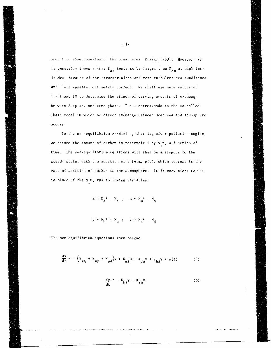
In the non-equilibrium condition, that is, after pollution begins,

we denote the amoun~t of carbon in reservoir i by Ni* a function of

time. The non-equilibrium equations will then be analogous to the

steady state, with the addition of a term, p(t), which represents the

rate of addition of carbon to the atmosphere. It is cocrvenient to use

in place of the N *, tne following variables:

x Na Na u m *-NM

y~N h*N h v vNd* N d

The non-equilibrium equations then become

dx (dt h am ad) ~ma da hy+Pt

dy K haY+ K ax (6)dt ha h

I! -K + K u -K x + K V(7)dt ma md a n drn

d v- v+K /+ K (8)dta dad" 'md(

Since we do not know the rate at which carbon fuel will be con-

sumed in the future, we must extrapolate the function p(t) from pres-

ent data. For the past few years world production of hydrocarbon fuels

has been increasing by over 4 percent per year, although the rate of

increase has not been steady as shown in Table 4.

Table 4

RECENT WORLD PRODUCTION OF HYDROCARBON FUELS

World Production Calculated

Coal Natural Gas Crude Petroleum Carbon "2leased

9 9 9 9Year (10 tons) (10 cu m) (10 tons) (10 tons)

1959 2.53 431 1.04 2.53

1960 2.64 479 1,12 2.67

1961 2.49 513 1.19 2.66

1962 2.55 547 1.30 2.79 9

1963 2.66 621. 1.39 2.97

1964 2.76 680 1.50 3.14

1965 2.81 723 1.62 3.28

1966 2.84 763 1.75 3.42

Production data from Bureau of Mines [1963-1966]. Natural gas liquids

are neglected, since they represent less than 2 percent of the total..

_ .

-13-

As long as the exponential rate of increase continues, the amount of

carbon released to the atmoaphere each year will have the form

p;) -Y 0 (e 't --1); 0 < t < t (9)

We shall assume t to be the year 1900, when thQ industrial revo-0

lution ,as gaining momentum and effluents to the atmosphere were be-

coming significant. The amount of carbon in the atmosphere at that

time, P , Is estimated to have been about 590 billion tons. Eviluating

the constants in Eq. (9) tc correspond with a 4 percent annual increase

and the production data f.)r 1966 gives:

(.0392

p(t) = .000471P0 (e -'1); 0 < t < t1 (10)

It is Linprobable that the exponential rate of increase in fuel

consumption will continue unabated until fuel supplies are completely

eohausted. It seems more likely that fuel consumption will continue

exponentially for some time, then level off as fossil fuel becomes

scarce and other types of energy are developed. Eventually the hydro-

carbor, tuels will cease to be significant a the last of the reserves

become unecnomical to recover. The leveling-off ?mrtion of the curve

may be approximated by a hyperbolic tangent function:

p(t) = c tanh bt; t .t ntmax etm dfu

The values for constants c and b will depend on the estimated fuel

-14-

consumption rate for many years in the future. If the rate of consump-

tion reaches a maximum of o times the current value, which was 3.42

billion tins per year in 1966, then c becomes .00578oP . For (tanh'0

bt) to approach a value of one within about 200 yr, b must be at least

0.01. The rquation for p(t) will then be

p(t) = .005 78pP tanh (.01 t); tI < t < t (12)O m ax

Larger values of b will cause the consumption rate to reach its maxi-

mum value sooner. Figure 2 illustrates the rate of carbon addition

to the atmosphere according to the scheme described above for 0 = 5,

10, 20. The exponential function is used to approximate the first

portion of the curve and the tanh function approximates the latter

half. The intersection of the two curves determines tI. Addition of

carbon is assumed to drop sharply to zero at t when all fossil fuelmax

resources are exhausted. The area under each composite curve represents

the total amount of carbon added over all time due to combustion of

fossil fuel, and in each case must be equal to the original supply

(4.9 P0 ). Thus thp integral determines the value of t m

t t tp(t)dt c, P 0 (e -)dt + Oa P m(tanh bt)dt 4.9 P (13)

00

-. 10-

Iw*41

'13

() u)

E .0

--

.0

4 w~

0 cro Q)

.0 43

"-4 L

o -4 0

0 41~00

E-44)

SNO 60 .0 0

-16-

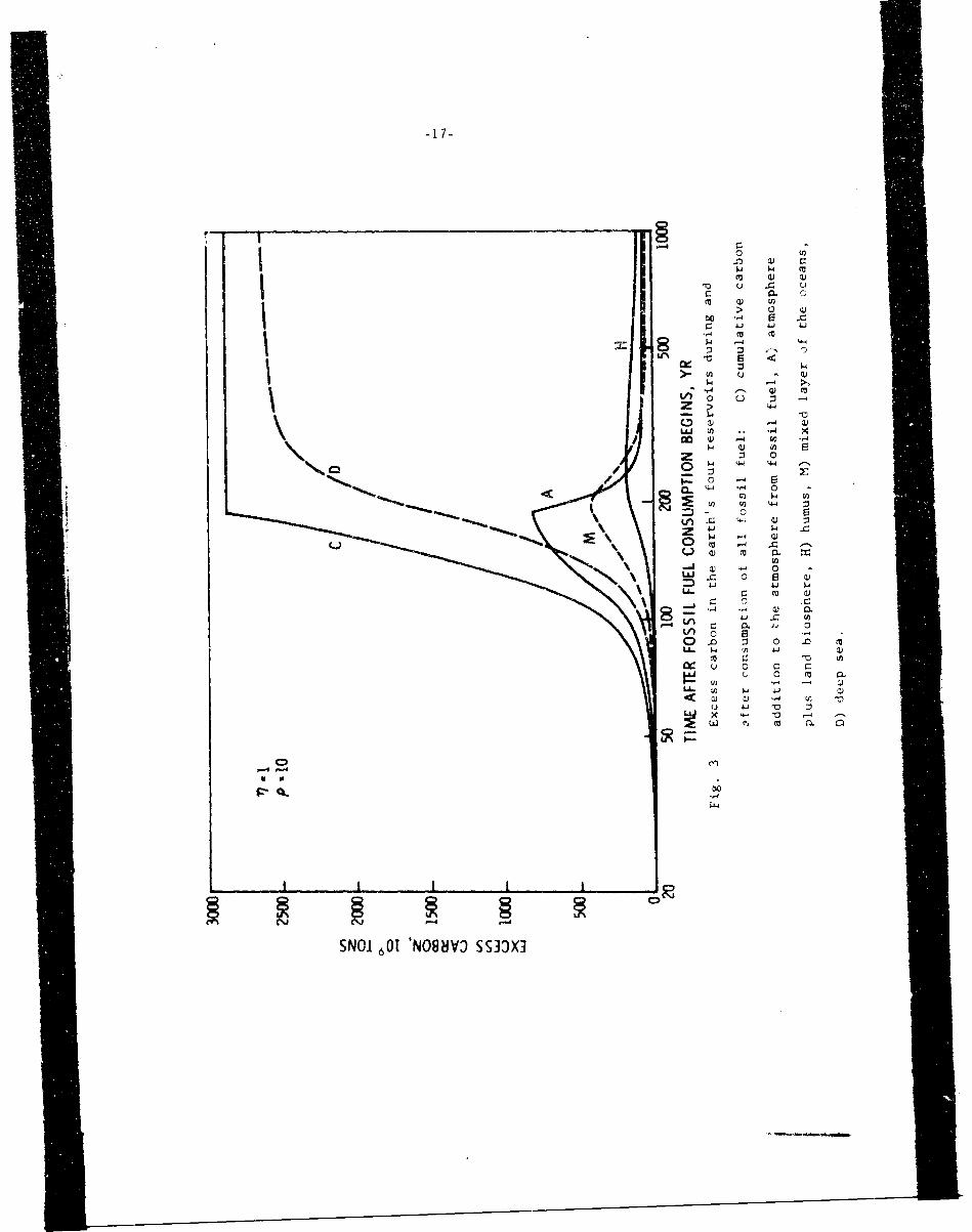
RES'TLTS

The rise and decay of excess carbon in the four reservoirs was

calculated by numerically integrating Eqs. (5) through (8) using sev-

eral assumptions as to the rate of consumption of fuel, total supply

of fossil fuel, and amount of mixing between deep sea and atmosphere.

Figure 3 illustrates the changes in carbon concentration in each

reservoir as excess carbon is added according to the schedule for

10. When the addition of carbon to the atmosphere stops (fuel

resources exhausted), the carbon concentration in each reservoir grad-

ually approaches a new equilibrium value, with over 90 percent of the

excess accumulating in the deep sea. In the case illustrated, the

atmosphere-land biosphere combined reaches a maximum carbon excess at

nearly the same time as the peak fuel consumption. The mixed layer

reaches a maximum about half as great a few years later. The ex-

cess carbon in the humus is even less and delayed somewhat longer than

the mixed layer, but over the long run it retains a slightly greater

quantity of carbon,

It was assumed that the exchange oetween land biosphere and at-

mospheru is fairly rapid, so that the ratio of carbon in these two

reservoirs remains essentially constant. Figure 4 illustrates the car-

bon content of the atmosphere alone for three different fuel consump-

tion rates. It can be seen that the maximum carbon content and the

time at which it is reached are highly sensitive to the value of 0'

The equilibrium value is independent of p, however, depending only on

the total amount of fuel .onsumed; thus th carbon content decays to

a value about 8 percent above normal in each case.

ca w (D

00 -,4 S e

-,44

>- Uc UU

1-4 .- >Ln ,. u ) C

ld~ o 4

C4 a)-

4-4 0 I

CCi

0A .n -

U- c

-C C C

LA 0 -4 0.

LA- -a c

0

SNOI 601 'NO8gVV SS33X]

u &W

0 cl

0.

/ m

co0 0Q) u

CL o w

0 m~El L)

4-1 --

-4A

c~J ece.

383HdSOWIV 1VWHON 01 3AIIY1M I1NON0 NOSUY3

-19-

A change in - has very little effect an the time variation of car-

bon in the atmosphere (Fig. 5). Changing has a greater, but opposite,

effect in the mixed layer an,,' also shifts the time of peak carbon con-

tent. The mixed layer reaches its maximum carbin content at t = 196

or 192 years for - = I or 10, respectively, while the atmosphere reaches

its maximum at t = 189 years in either case, giving delay tinmes A 7

years for - = I or 3 years for = 10.

The inclusion of shale oil extends the total fossil fuel supply

slightiy (10 years for c = 10), but as Fig. 6 shows, it has a rela-

tively minor effect on the carbon content of the atmosphere. The ul-

timate equilibrium value after all fuel Ls consumed is about 10 percent

higher tht:n if shale o,1 were not included.

We may conclude that Lhe atmnspheric carbon concentration is not

highly sensitive to the discrepancies in estimating total fuel re-

sources, nor to variations in direct exchange between atmosphere and

deep sea, )ut that the rate of future fuel consumption is much more

critical to the transient cdrb,.n distribution.

2' C

C>-

x0

**

cl-c

IVW80N 01 3AlIV138 1NIUN0O N098V

-2LA-

I -

] ]HS(M V 1'W8N 0IAI-13 N NO 08V

-22-

DI2SCUSSION

Acccrding to the mo,. of carbon exchange described here, abo',t

40 percent of the carbon released so .ar buy combustion of fossil fuel

should have remained in the atmoephere, This is iii reasonable agree-

ment with the data of Keeling and Waterman F1968], whose measurements

indicate that the increase in atmospheric carbon dioxide corresponds

to about half the carbon fuel consumed to date. The model further

indicates that the natural exchange processes among carbon reservoirs

cannot operate fast enough to maintain equilibrium as long as the cur-

rent and projected rates of fossil fuel consumption prevail. Thus, it

may be expected that the armosphere will continue to accumulate nearly

halt of the carbon ;eleased until fuel consumption rates decline or

the fuel supply is exhiustej. It i. impossible to predict with any

confidence the meximum carbon dioxide concentration that will be reached,

since that depends on future rates of hydrocarbon fuel consumption.

Obviously the scheme -resented here for describing future consumption

rates is only one of many possibilities. However, within the con-

straints of the known recent consumption rates and the remaining sup-

ply, it would seem that future con;umption rates could not deviate

greatly irom those presented here. In any case, it appears that the

equilibrium concentvation of carbon in the atmosphere that is eventu-

ally reached after all fossil fuel is consumed will be about 8 percent

above the pre-1900 normal.

-23-

REFERENCES

Averitz, Paul, U.S. Department of the Interior, Geological S:rvey

News Release, April 20, 1968.

Bolin, B., and C. D. Keeling, Large Scale Atmospheric Mixing, J. Geo-

phys. Res., 68 (13), 3899-3920, 1963.

Bureau of Mines, U.S. Department of the Interior, Bull. #630, Mineral

Facts and Problems (1965).

Bureau of Mines, U.S. Department of the Interior, Minerals Yearbook,

1963-1966.

Callendar, G. S., On the Amount of Carbon Dioxide in the Atmosphere,

Tellus, i0. 243-248, 1958.

Craig, H., The Natural Distribution of Radiocarbon: Mixing Rates in

the Sea and Residence Times of Carbon and Water, in Earth Science

and Meteoritics, edited by J. Geiss and E. D. Goldberg, pp. 103-114,

North Holland Pub. Co., Amsterdam, 1963.

Hendricks, T. A., Resources of Oil Gas and Natural Gas Liquids in the

U.S. and the World, U.S. Geological Survey circular #522 (1965).

Hubbert, M. K., Energy Resources, National Academy of Sciences - Na-

tional Research Council Publication 1O00-D, Washington, D.C., 1962.

Keeling, C, D., and L. S. Waterman, Carbon Dioxide in Surface Ocean

Waters, J. Geophys. Res. 73 (14), 4529-4541, 1968.

Plesset, M. S., and D. J. Dugas, Decay of a Disturbance in the Natural

Distribution of Carbon-14, The RAND Corporation, RM-5'OO1-TAB, November

1966.

---------... .

-24-

Weeks, L. G,, The Next Hundred Years Energy Demand and So:LrL,,s of

Supply, GeoTimes, 5, (1), 18-21 and 51-.55, 1960.