ii.3.2 rapid prediction of co2 movement in aquifers, coal ... · ii.3.2 rapid prediction of co2...

$: II.3.2 Rapid Prediction of CO2 Movement in Aquifers, Coal ... · II.3.2 Rapid Prediction of CO2 Movement in Aquifers, Coal Beds, ... Mass transfer between the matrix and fracture$
II.3 Project Results: Geologic CO2 Sequestration

GCEP Technical Report - 2004 115

II.3.2 Rapid Prediction of CO2 Movement in Aquifers, Coal Beds, and Oil and Gas Reservoirs

Investigators A. R. Kovscek, Associate Professor, Petroleum Engineering; F. M. Orr Jr, Professor, Petroleum Engineering Department; K. Jessen, Acting Assistant Professor, Petroleum Engineering Department, G. Q. Tang, Research Associate, M. D. Cakici, Marc Hesse, C. J. Seto, Graduate Research Assistants Background

Considerable effort has been devoted to the development of reservoir simulation tools for the oil industry, and there are high-quality simulators available that handle effectively many of the flow problems appropriate to oil and gas reservoirs. One area where simulator development is continuing, however, is in the simulation of processes in which multiple components transfer between whatever phases are present in the porous medium. Injection of CO2 into geologic reservoirs inevitably involves such component transfers, as the injected CO2 dissolves in any water or oil present, as hydrocarbons transfer to the relatively dense CO2-rich phase, or as CO2, methane, and possibly N2 adsorb and desorb in coal.

Because the most important physical mechanisms of storage differ for the three geologic systems, it is appropriate to consider the current state of predictive models for each setting. Compositional simulation tools are best developed for oil and gas reservoir settings, for which several fully capable finite-difference compositional simulators are available. ECLIPSE 300 and GEM are examples. These codes use an equation of state to represent equilibrium partitioning of components between oil and gas phases, and they handle the effects of capillary pressure and gravity well. The principle limitations of these simulation tools are computation speed and the adverse effects of numerical dispersion on computed composition path. For aquifer and coalbed settings there are also several simulation tools available. The capabilities of some of them are reviewed in the paragraphs that follow.

TOUGH2 is a numerical simulator for non-isothermal flows of multicomponent,

multiphase fluids in one-, two-, and three-dimensional porous and fractured media20. TOUGH2 was originally developed for geothermal reservoir engineering, nuclear waste disposal and hydrology. There are several simulators in the TOUGH2 family that include physical mechanisms appropriate to CO2 sequestration in aquifers, including TOUGHREACT/ECO2 (includes transport of aqueous liquid and vapor phases by advection, chemical reactions for dissolved species and minerals, and molecular diffusion in both liquid and gas phases), ChemTOUGH (implicit formulation that allows larger time steps but requires substantially more memory), and TOUGH2-FLAC3D (couples TOUGH2/ECO2 with FLAC3D which models rock and soil mechanics). This family of simulators generally makes use of the equilibrium assumption: components equilibrate rapidly among whatever phases are present. An exception is made for mineral dissolution and precipitation, which can be modeled as in local equilibrium or subject to a kinetic model.


116 GCEP Technical Report - 2004

NUFT30 is an integrated software package containing five application specific modules, for the simulation of multiphase and multicomponent flow and reactive transport within a wide range of subsurface environments. The code can model multiphase advection, diffusion, dispersion, relative permeability, and kinetically controlled fluid-mineral reactions. The feedback between transport and geochemical reactions can be modeled by dependence of the permeability on porosity changes due to reactions. PVT properties of CO2 and water are calculated from equation of state formulations. The SUPCRT92 software package is used for calculation of fluid mineral equilibria31. It provides standard state thermodynamic data and equilibrium constants for a wide range of minerals, gases, and aqueous species over a wide range of temperatures and pressures.

FLOTRAN32 describes coupled thermal-hydrologic-chemical processes in variably

saturated, nonisothermal, porous media in three dimensions. FLOTRAN describes systems involving two-phase fluid flow and multicomponent reactive chemical transport involving aqueous, gaseous, and mineral species. FLOTRAN includes separate modules that handle the mass and energy transport and the reactive transport. FLOW solves the mass conservation equations for water and gas and energy. TRANS solves mass conservation equations for a multicomponent geochemical system. Effects of capillary, gravity, and viscous forces are included, as are energy transport by convection and conduction. The equilibrium assumption is made for chemical reactions, with kinetic representations available for mineral dissolution and reaction. Changes in porosity and permeability can be represented.

STOMP33 is a computer model for simulating subsurface flow and transport. Solute

transport, radioactive decay, and first-order chemical reactions modeled, following the solution of the coupled flow equations. Reactions and transport are coupled to the flow by accounting for changes in host rock porosity and permeability. An equation of state for CO2 is included that handles a wide range of temperatures and pressures to 800 bars. Options appropriate to sequestration include H2O-CO2-NaCl, H2O-CO2-NaCl-Energy, H2O-CO2-CH4-NaCl, and H2O-CO2-CH4-NaCl-Energy. Extension to account for other geochemical reactions is planned.

The UTCOMP simulator is a three-dimensional, isothermal, equation-of-state

compositional simulator34. The simulator can be used to study the effects of physical dispersion, gravity, reservoir heterogeneity, phase behavior, fingering, relative permeability and capillary pressure effects including capillary number, and reactive and partitioning tracers. A maximum of four phases is permitted to co-exist, including one aqueous phase and three hydrocarbon phases. Local thermodynamic equilibrium between hydrocarbon phases is assumed with the exception of rate-limited mass transfer of surfactant between phases, rate-limited mass transfer of hydrocarbons into a flowing gas phase and reactive tracers. UTCOMP was written to simulate enhanced oil recovery, and several modifications are needed in order to simulate CO2 sequestration. For CO2 injection into aquifers, phase 2 was used for the aqueous phase, and phase 3 was the gas phase (supercritical CO2 plus some H2O as a dense fluid phase). Phase equilibrium in the binary CO2-H2O mixtures in each grid block is calculated using the Peng-Robinson



equation of state. The effect of salinity on the solubility of CO2 in brine is modeled by adjusting the binary interaction coefficients in the Peng-Robinson equation. Henry's law is used to model the solubility of CO2 in water, including a correction for salinity of the brine.

Coalbed methane (CBM) simulators also model physical mechanisms thought to be

important in CBE recovery and CO2 storage processes: the dual porosity structure of the coal bed, adsorption/desorption of CH4 at the coal surface, coal matrix shrinkage due to CH4 desorption, and diffusion of gas from the matrix to the fracture system. Additional physical mechanisms that may play a role in CO2 storage on coalbeds include: coal matrix swelling due to CO2 adsorption onto the coal surface, mixed gas adsorption, and diffusion of multiple gas components.

Enhanced CBM simulators that are applicable to CO2 storage can be divided into two groups: those that use a compositional framework, and those that adopt a black oil framework. In the compositional framework, fluid properties are rigorously modeled based on an equation of state. In the black oil framework, fluid properties are supplied by lookup tables obtained through laboratory work or correlations. Compositional Framework

PSU-COALCOMP35 is a compositional, dual porosity coal bed methane simulator that accounts for multi-component sorption and transport phenomena. Multicomponent sorption is modeled via an ideal adsorbed solution theory and the Peng-Robinson equation of state. Mass transfer between the matrix and fracture system is defined via a sorption time constant, a lumped parameter that incorporates diffusion time, rate or sorption/desorption and cleat spacing of the coal.

GCOMP a simulator that assumes instantaneous diffusion between the matrix and the fracture systems, allowing reduction of the system to a single porosity system36. Mixed gas adsorption is modeled via an extended Langmuir model. In this approach, the concentration of each gas component is a function of its partial pressure. Geomechanical effects on permeability and porosity are modeled, as is coal matrix shrinkage and swelling due to adsorption/desorption of gases on the coal surface.

SIMED II is a two-phase multicomponent single or dual porosity coal bed reservoir simulator37. The Peng-Robinson equation of state is used to calculate fluid properties. Water phase properties are evaluated internally. Multiphase gas adsorption can be modeled via an extended Langmuir isotherm or an ideal adsorbed solution model. Stress-dependent permeability and porosity can be accounted for through a choice of one of five models. SIMED II also accounts for geomechanical effects associated with injection. A dynamic fracture model represents the initiation and growth of injection-induced hydraulic fractures.

CMG-GEM38 is another multiphase, multicomponent single of dual porosity coal bed reservoir simulator. Phase behavior can be described by either the Peng-Robinson or Soave-Redlich-Kwong equation of state. Shape factors can be used to account for flow



between porosities, and additional transfer enhancements can be used to account for fluid placement in the fractures. Mixed gas adsorption is modeled via an extended Langmuir isotherm, and the corresponding diffusion model can be selected base on either concentrations calculated from adsorption characteristics or based on free gas properties. Stress dependent relative permeability changes and matrix swelling and shrinkage can be included.

METSIM239,40 is a 3D multicomponent, triple porosity coal bed reservoir simulator.

This formulation assumes that there is no water present in macropore system, only free gas exists, and its transport is diffusion controlled. This formulation allows for the competitive desporption in coal by specifying different diffusion time constants for the macropore and the micropore systems. Gas properties are calculated using an equation of state. Multicomponent adsorption is described using an extended Langmuir model. METSIM2 is also coupled to a wellbore and rock mechanics simulator, allowing pore pressure dependent permeability functionality. Black Oil Framework

COMET3 is an extension of COMET and COMET2, developed to model low-rank coal and water saturated gas-shale reservoirs41. It can model single, dual, and triple porosity approximation of the coal bed system. In the triple porosity system, gas desorbs from the internal matrix, and migrates to the micropermeability matrix and finally to the cleat system where it flows to the wellbore. In this formulation, the micropermeability matrix system also models multiphase effects. This accounts for the establishment of a critical gas saturation in the matrix, which may be responsible for a delay in early time gas production observed in some fields. Desorption and diffusion is explicitly modeled. COMET3 can model multiple gas components and accounts for different diffusion rates of the components. An extended Langmuir isotherm is used to model mixed gas adsorption. Pore volume compressibility accounts for stress-dependent porosity and permeability changes. A differential swelling model based on laboratory experiments accounts for swelling attributed to non-CH4 components of the gas.

ECLIPSE-10042 is a black oil simulator with additional features for modeling CBM. A dual porosity system is used to model the coal bed system. This simulator is only able to handle two gas components, and therefore it is not able to model an ECBM process with flue gas injection. Compositional effects between CO2 and CH4 are handled by introducing a "solvent" phase. Adsorption is described by the Langmuir isotherm. Eclipse-100 can account for coal shrinkage and compaction effects.

The simulators currently available for aquifer and coalbed storage of CO2 are very capable, with many physical mechanisms represented. They will continue to be very useful for exploring the interplay of physical mechanisms for computational grids of limited size, but they are subject to significant limitations for application at field scale. Conventional finite-difference compositional simulations, even with relatively small numbers of components, are too slow to handle high-resolution representation of the spatial distribution of permeability at field scale, and when coarse computational grids are used instead, they are badly affected by numerical diffusion, which can alter



calculated composition paths in a way that affects calculated performance significantly. Hence, they are probably not suitable for routine simulation of field-scale flows at grid resolutions sufficient to capture the effects of preferential flow paths created by reservoir heterogeneity, especially if the impact of variability in the permeability distribution is to be assessed. For screening of sites, assessment of areas invaded by CO2, or rapid exploration of the impact of injection well placement, simulation tools that are significantly more efficient, but necessarily more limited in the mechanisms represented, are appropriate. One approach, the use of streamline methods, is demonstrated next for two of the geologic settings, gas reservoirs, and aquifers. In the section that follows, we also consider the time scales for dissolution of CO2 in brine in an aquifer and for the equilibration of gas adsorption in a coal bed, summarize work to examine the cooptimization of CO2 storage and performance of an oil recovery process, and we report results of coal adsorption experiments. Results

Compositional streamline methods are based on the idea that the flow can be represented as a series of one-dimensional solutions for multiphase, multicomponent flow along each streamline, with the locations of the streamlines capturing the effects of permeability heterogeneity. In reservoir flows that are dominated by heterogeneity, streamlines move little, and hence streamline locations need be updated only occasionally. In those settings, the streamline approach can be orders of magnitude faster than conventional finite difference computations because the largest computational cost is associated with solving the pressure equation for the streamlines. Effects of gravity segregation and capillary crossflow are not represented in the basic streamline approach, a significant limitation for some reservoir settings. Several investigators have shown that it is possible to represent effects of gravity and capillary pressure in streamline computations by operator-splitting techniques. This approach is reasonable as long as very frequent streamline updates are not needed. Frequent streamline updates are subject to errors that arise from mapping and remapping streamlines, and they eliminate the speed advantage of the approach.

Combined CO2 Storage and Condensate Vaporization

CO2 injection into a gas reservoir is a process that can be modeled well by a streamline calculation. The viscosity contrast between injected gas and the gas and condensate in place in the reservoir is small (and the mobility ratio is favorable), and density differences are also relatively small, so streamlines change location slowly compared to the rate at which composition fronts move. The local equilibrium assumption (that fluid phases present at a given location are in chemical equilibrium) is also reasonable for this setting.

To test the use of streamline simulation for CO2 injection in a gas reservoir in which

condensate dropout had occurred, we compared streamline simulations with results of ECLIPSE-300 simulations for the same system. In this example, we did not include effects of gravity segregation or capillary crossflow. Analysis of the scaling of these crossflow phenomena suggested that capillary effects were small enough to be neglected,



while gravity effects somewhat larger but still small enough that testing the use of the streamline in the absence of a representation of gravity segregation was reasonable43.

Displacement of a 13-component system was considered. Fluid properties and

equation-of-state characterization for the fluid system are reported by Jessen and Orr1. The analytical solution for one-dimensional displacement of this fluid system by pure CO2 is shown in Figure 13. As the injected CO2 propagates through the porous medium, it vaporizes condensate, creating a bank of hydrocarbon liquid at the leading edge of the transition zone. The analytical solution is compared in Figure 13 with a series of finite difference simulations for the same problem, with grid resolutions of 100, 500, 1000, and 5000 grid blocks. Comparison of the numerical and analytical solutions indicates that for this compositional problem, the numerical dispersion present in the FD solutions does not resolve the condensate bank unless a very fine grid is used. It is unlikely that use of such fine grids would be attempted in field-scale compositional simulations because the computation times required would be unacceptably large.

Figure 13: Comparison of analytical solution for 1D displacement of a 13-component gas condensate system by pure CO2.

Three finite difference simulations, using identical permeability fields, were performed to assess the magnitude of gravitational effects in this displacement:

• Permeability field oriented vertically, injection at a rate advance of 1.4 m/d (low rate case).

• Permeability field oriented vertically, injection at a rate of advance of 2.8 m/d (high rate case).

0.86

0.88

0.9

0.92

0.94

0.96

0.98

1

1.02

0 0.5 1 1.5 2

wave velocity (z/t)

gas

satu

ratio

n (fr

ac.)

MOCFD 100FD 500FD 1000FD 5000



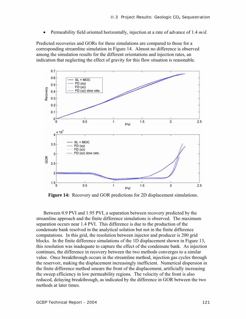
• Permeability field oriented horizontally, injection at a rate of advance of 1.4 m/d. Predicted recoveries and GORs for these simulations are compared to those for a corresponding streamline simulation in Figure 14. Almost no difference is observed among the simulation results for the different orientations and injection rates, an indication that neglecting the effect of gravity for this flow situation is reasonable.

Figure 14: Recovery and GOR predictions for 2D displacement simulations.

Between 0.9 PVI and 1.95 PVI, a separation between recovery predicted by the streamline approach and the finite difference simulations is observed. The maximum separation occurs near 1.4 PVI. This difference is due to the production of the condensate bank resolved in the analytical solution but not in the finite difference computations. In this grid, the resolution between injector and producer is 200 grid blocks. In the finite difference simulations of the 1D displacement shown in Figure 13, this resolution was inadequate to capture the effect of the condensate bank. As injection continues, the difference in recovery between the two methods converges to a similar value. Once breakthrough occurs in the streamline method, injection gas cycles through the reservoir, making the displacement increasingly inefficient. Numerical dispersion in the finite difference method smears the front of the displacement, artificially increasing the sweep efficiency in low permeability regions. The velocity of the front is also reduced, delaying breakthrough, as indicated by the difference in GOR between the two methods at later times.



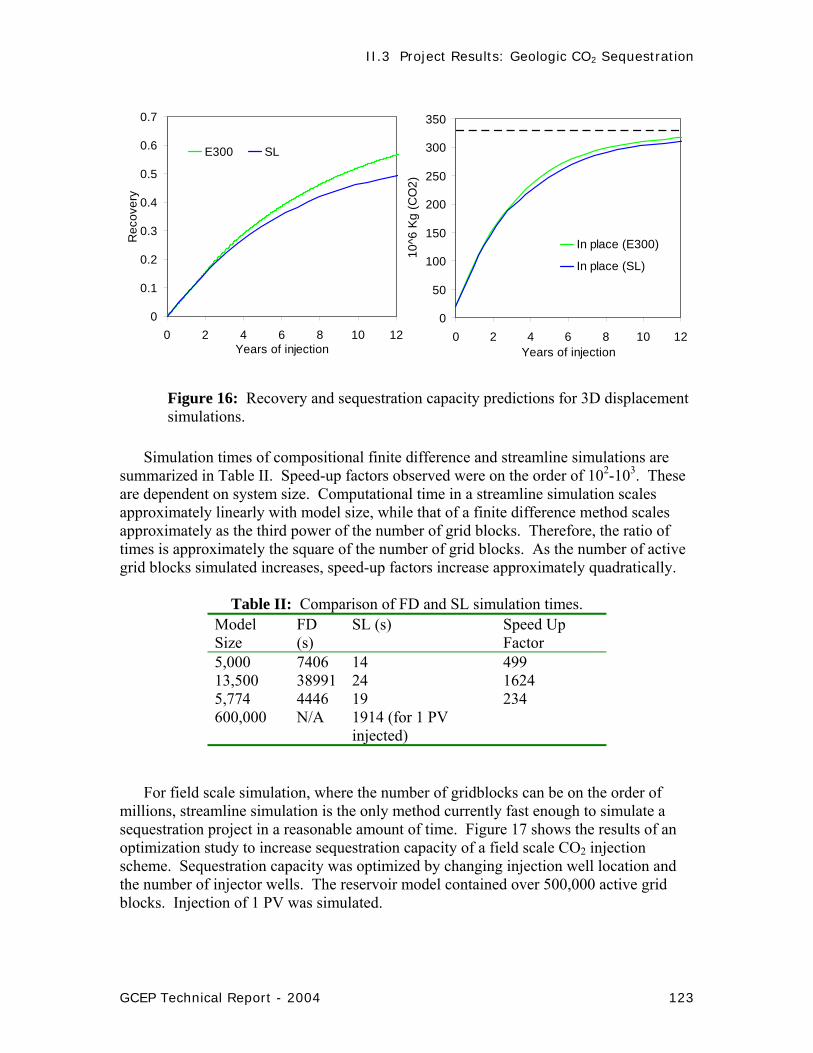
A 3D sector model representing a multi-well gas injection scheme was simulated. The permeability field and well locations for this displacement are shown in Figure 15. Corresponding recovery and total CO2 storage curves for the sector model are shown in Figure 16. Breakthrough occurs slightly earlier when the displacement is simulated using streamlines. Again, this is related to formation of high flow zones once the displacement front reaches a producer. CO2 bypasses condensate in the upswept areas resulting in a lower recovery, but high local displacement efficiency in the swept zones. In the FD simulation, dispersion creates a larger reservoir area contacted by the injected CO2 while the local displacement efficiency in parts of the swept zones is fairly low. The trade-off between sweep efficiency and local displacement efficiency results, for this case, in a higher recovery prediction by the FD simulation, which may very well be artificially optimistic. While the finite difference method and streamline method represent two end members of process recovery (due to low dispersion effects in a condensate displacement), it is likely that the dispersion-free solution used in the streamline calculation more accurately predicts process recovery. The lower sequestration capacity (Figure 16) predicted by the streamline approach is again due to the lower sweep efficiency, a conservative estimate in this example.

Figure 15: Permeability field and well locations for a 3D sector displacement.

I1

ln (md)

P5

P4

P3

P2

P1



0

0.1

0.2

0.3

0.4

0.5

0.6

0.7

0 2 4 6 8 10 12Years of injection

Rec

over

yE300 SL

0

50

100

150

200

250

300

350

0 2 4 6 8 10 12Years of injection

10^6

Kg

(CO

2)

In place (E300)

In place (SL)

Figure 16: Recovery and sequestration capacity predictions for 3D displacement simulations.

Simulation times of compositional finite difference and streamline simulations are

summarized in Table II. Speed-up factors observed were on the order of 102-103. These are dependent on system size. Computational time in a streamline simulation scales approximately linearly with model size, while that of a finite difference method scales approximately as the third power of the number of grid blocks. Therefore, the ratio of times is approximately the square of the number of grid blocks. As the number of active grid blocks simulated increases, speed-up factors increase approximately quadratically.

Table II: Comparison of FD and SL simulation times. Model Size

FD (s)

SL (s) Speed Up Factor

5,000 7406 14 499 13,500 38991 24 1624 5,774 4446 19 234 600,000 N/A 1914 (for 1 PV

injected)

For field scale simulation, where the number of gridblocks can be on the order of millions, streamline simulation is the only method currently fast enough to simulate a sequestration project in a reasonable amount of time. Figure 17 shows the results of an optimization study to increase sequestration capacity of a field scale CO2 injection scheme. Sequestration capacity was optimized by changing injection well location and the number of injector wells. The reservoir model contained over 500,000 active grid blocks. Injection of 1 PV was simulated.



0

0.1

0.2

0.3

0.00 0.25 0.50 0.75 1.00 1.25PVI

Rec

over

y

case 1case 2case 3case 4

0

10

20

30

40

50

0.00 0.25 0.50 0.75 1.00 1.25PVI

CO

2 in

pla

ce (1

0^6

ton)

case 1case 2case 3case 4

Figure 17: Field scale optimization study to maximize production and sequestration capacity. Reservoir model had over 500,000 active grid blocks. Run time of each streamline simulation was less than 10 minutes.

Cooptimization of CO2 Storage and Enhanced Oil Recovery Previous work demonstrated that the design of combined EOR and sequestration

operations differs significantly from the design for EOR alone. For pure EOR, the objective is to maximize oil recovery, while injecting minimum CO2, and this is typically accomplished by injecting water in some version of a water-alternating gas process. In combined sequestration and EOR, oil recovery and the amount of reservoir volume filled with CO2 are both to be optimized. Last year’s report summarized our efforts in cooptimization (see also Cakici44)

To examine further the cooptimization question, we used a realistic 3D,

heterogeneous, and stochastic reservoir description including a 15-component reservoir fluid. These computations were performed using ECLIPSE-300. The reservoir shape is anticlinal, and it is bounded by faults and an aquifer. There are four injectors near the flanks of the reservoir and 4 producers near the crest. The oil is relatively heavy



(24°API), and pure CO2 is not miscible in the crude oil at reservoir pressure. A well control scheme was implemented in the simulator that actively shuts in producers with large gas to liquid producing ratios. This scheme allows gas injection without any water injection. Water injection frustrates cooptimization efforts by filling pore space that could otherwise be utilized for sequestration. Control of wells in this fashion allows the same amount of oil to be produced as in an optimized WAG process (with pure CO2 as the injectant) while simultaneously storing about 2.5 times as much CO2 as compared to the WAG.

Despite these promising results, questions existed as to whether the well-control scheme was robust and whether the results obtained with the well control were overly sensitive to the distribution of heterogeneities in the reservoir model. The parameters used to operate the production well are producing gas-oil ratio, injection pressure, and an increase in the allowed producing gas-oil ratio each time a producer is allowed to flow. The initial producing gas-oil ratio and the increment to the gas-oil ratio were chosen in an ad hoc fashion. The sensitivity of performance to values of the allowed gas-oil ratio and its increment were examined through further simulation.

Figure 18 presents the results for the sensitivity analysis of pure CO2 injection by plotting the variation in the net cumulative recovery, Figure 18a, and reservoir utilization functions, Figure 18b. The y-axis is the producing gas-oil ratio where the production well is first shut in, whereas the x-axis is the increment made to the producing gas oil ratio each time an injection well reaches maximum pressure (350 bar), and producers must be opened to prevent overpressurization of the reservoir. Gray shading represents relatively low values of recovery or utilization, and white represents relatively greater values.

On the one hand, Figure18 teaches that optimal well control is obtained when the gas-

oil ratio where the well is first shut in is set to just slightly above the solution gas-oil ratio (that is the solubility of gas in the oil). This allows control of gas flow at just about the time that gas breaks through to the injection well. Similarly, the results show that increment to the producing gas-oil ratio should be made as small as practical to obtain the best performance.

On the other hand, these results also show that performance of the well-control scheme does not depend critically on control parameters. Note the variations in maximum and minimum values. Differences in recovery and utilization among "best" and "worst" parameters settings differ by 6% to 14%. Thus, the sensitivity analysis indicates that producing gas-oil ratio and injection pressure are robust control parameters. This well-control strategy does not appear to require a high degree of parameter tuning to obtain beneficial results.

Similarly, the sensitivity of results obtained with the well-control scheme was examined as a function of the distribution of permeability within the 3D reservoir model. The injection scenarios include: pure CO2 injection, WAG with 0.01 PV slugs of CO2



(a)

(b) Figure 18: Sensitivity of (a) net cumulative recovery and (b) reservoir utilization results to well-control parameters. Pure CO2 is injected into 3D reservoir model.



and water, CO2 injection with well control, and solvent gas (2/3 CO2 and 1/3 C2) injection with well control. Results showed that the oil recovery increased or decreased from model to model, but the best performing production scenario for any given reservoir model is well-controlled injection of solvent. With respect to reservoir utilization, well control with pure CO2 injection sequesters the most CO2. WAG does lead to different sorting of the performances among the reservoir models; however, these deviations from the reference case do not change the conclusion that the well-controlled cases are preferred for cooptimization.

Time Scales for CO2 Dissolution in Brine

At the pressures and temperatures encountered in saline aquifers, the injected CO2 will form a buoyant gas phase, which will therefore migrate back towards the surface unless migration is inhibited by a geological barrier to vertical flow. To understand whether and if so how much CO2 might be available to flow vertically, we need to understand how long the injected CO2 will be mobile. Therefore, we need to understand trapping mechanisms that prevent upward migration by CO2 and the time-scales over which they operate. If the CO2 gas phase moves due to its buoyancy or is displaced by invading brine, gaseous CO2 may be trapped as an isolated residual CO2 phase. This mechanism will be referred to below as residual trapping. CO2 has a modest solubility in the aqueous phase, the aqueous CO2 increases the density of the brine slightly4, and therefore brine containing dissolved CO2 will sink rather than rise. We will refer to this trapping mechanism as solution trapping. Figure 19 shows sketches of possible configurations of CO2 in an aquifer.

Figure 19: Schematic of CO2 dissolution in two aquifers. The mobile CO2 gas phase is dark blue, the dissolved aqueous CO2 is light blue, residual CO2 is orange, and the brine is not colored. a) CO2 gas is held under a structural trap. Dissolution of CO2 into the brine reduces the CO2 phase volume. b) The CO2 gas phase migrates along the top of a sloping aquifer, and leaves behind a region of residual CO2. In this case both dissolution and residual CO2 saturation contribute to the decrease of the mobile CO2 phase.

Reactions of dissolved CO2 with cations in the brine may ultimately lead to the precipitation of minerals, depending on brine chemistry and aquifer mineral content.



These geochemical reactions have rate constants low enough45 that mineralization reactions will not contribute volumetrically to the trapping of CO2 in the first several hundred years. However, small changes in porosity due to precipitation may significantly decrease the permeability and help to trap the CO2 plume dynamically. Residual and dissolution trapping are therefore the likely mechanisms that decrease the amount of mobile CO2 within the first several 100 years. Residual trapping will only be important if the CO2 plume moves through the aquifer, and water invades zones containing gas, a likely event as CO2 from the gas phase transfers to the brine. Dissolution trapping will contribute when CO2 gas phase is in contact with the brine. Convection Enhanced Dissolution

At the interface between gaseous CO2 and the brine, CO2 dissolves into the brine. This dissolution is fast enough that it can be considered to be at equilibrium. The rate of CO2 dissolution is therefore determined by the transport of CO2 away from the interface. In the absence of advection, the aqueous CO2 has to diffuse away from the interface. Ennis-King and Paterson4 have estimated that the minimum time until a given CO2 layer is dissolved by diffusion alone as

DL

Diff

2~ ατ , (1)

where α~10 is the ratio of the density in the gas phase CO2 to the mass of CO2 per unit volume of brine containing dissolved CO2, D ~ 10-9 m2/s is the molecular diffusion coefficient, L is the thickness of the initial layer of gaseous CO2. For L ~ 10 m the minimum time for dissolution of all CO2 is of the order of 1 million years. Advective transport of CO2 away from the interface could increase the rate of CO2 dissolution and decrease the dissolution time scale by orders of magnitude.

Ennis-King and Paterson4 report an increase of brine density with increasing aqueous CO2 concentration. This allows convective transport of CO2 away from the interface due to buoyancy-driven convection. They argue that the minimum time for dissolution in this case is given by the time it takes for the heavy fingers to propagate a distance αL. Assuming a gravitational velocity ug ~ g∆ρk/µ where g is the gravitational acceleration, ∆ρ is the density difference, k is the permeability and µ is the viscosity of the brine, the time for convective mixing is at least

~mixL

gkα µτ

ρ∆ . (2)

For common aquifers, this time scale is on the order of 104 - 105 yrs, up to two orders of magnitude shorter than the diffusive time scale. Gravity-driven convection may therefore enhance CO2 dissolution significantly, if it occurs. Convection will only be an effective transport mechanism if fingers of dense CO2 can migrate significant distances before diffusion eliminates the concentration and hence the density difference. For a



disturbance with distance d between adjacent fingers, the diffusive time scale for cross-finger transport is

( )D

dcross

22/~τ , (3)

so that the length scale of vertical finger propagation is at least

2 132 2

4 9

10 10 5 24 4 6 10 10f g cross

gkdL u d dD

ρτµ

−

− −

∆ ⋅ ⋅≥ = = ≈

⋅ ⋅ ⋅. (4)

Depending on the wavelength of the disturbance d, Lf may be smaller or bigger than the required distance for dissolving all CO2 given by αL.

A mathematical analysis of the instability of the diffusive boundary layer can determine the circumstance under which the diffusive boundary layer will become unstable, subject to the assumptions and boundary conditions used, of course, and give some insight in the initial length scale of the disturbances. Ennis-King and Paterson have presented such a stability analysis of the diffusive boundary layer at the interface between the gaseous CO2 and the brine4. They also performed numerical simulations with the TOUGH2 code20 that show propagation of CO2 fingers over tens of meters in 103 to 104 years. However, the simulations were affected significantly by numerical dispersion, and the numerical grid had a similar or larger length scale than the instabilities in their simulation results. We have reproduced and checked their stability analysis and translated it back into physical space.

To analyze the stability of the boundary layer mathematically, Ennis-King and

Paterson have assumed an infinite, homogenous, horizontal layer of depth H. The gaseous CO2 layer supplying the aqueous CO2 is neglected. This is a reasonable assumption, because the gravitational instability is between two miscible phases, brine and heavier brine with dissolved aqueous CO2. They further assume that the density change is small enough so that it can be neglected in all terms except the gravitational term, this is also called the Boussinesq approximation. The governing equations are therefore:

0u∇ ⋅ =v , (5)

( )zegPKu ˆρµ

−∇⋅−=v , (6)

CDCutC 2∇=∇⋅+

∂∂ φφ v , (7)

where ),,( wvuu =v is the Darcy velocity, P is the pressure, K is a diagonal permeability tensor that may be anisotropic (kx = ky ≠ kz), µ is the viscosity of the fluid, ρ(C) is the density of the fluid, g is the gravitational acceleration, C is the concentration of aqueous



CO2, φ is the porosity of the porous medium, and D is the coefficient of molecular diffusion of aqueous CO2 in water. The initial state that is considered is supposed to represent the aquifer some time after CO2 injection has stopped, and the system has come to rest. The initial condition is therefore 0),0( == xtu vv , and initially there is no dissolved CO2 in the brine, hence 0),0( == xtC v . The boundary conditions are no penetration for the vertical component of the velocity w(z = 0,t) = w(z = H,t) = 0 and the concentration has mixed inhomogeneous boundary conditions C(z = 0; t) = 0=

=∂∂

HzzC . Choosing the

following characteristic scales Cc = C0, tc = H2/D, xc = yc = H/γ1/2, zc = H, uc = vc = φD/(Hγ1/2), wc = φD/H and pressure is scaled by Pc = µφD/kv, where γ = kz/kx is the permeability anisotropy, the dimensionless governing equations are

0=⋅∇ uv , (8)

RaCPu γ+−∇=v , (9)

2

22

zCCCu

tC

H ∂∂

+∇=∇⋅+∂∂ γv , (10)

where 2

2

2

22yxH ∂

∂∂∂ +=∇ , and D

Hkg hRa µϕρ∆= is the Rayleigh-Darcy number. The governing

equations only depend on two parameters, the permeability anisotropy γ and the Rayleigh-Darcy number Ra. The initial and boundary conditions for the advection diffusion equation admit the following transient base state solution,

( )( ) ( )∑∞

=

−− ⎟⎠⎞

⎜⎝⎛ −

−−=

1

2/12

122

sin12

141),(n

tnb ezn

nztC ππ

π. (11)

To study the stability of this base state solution, we introduce small perturbations in

concentration and velocity. First we linearize the perturbed equations and subtract the base state. Then we make the plane wave approximation for the shape of the disturbances and obtain two coupled partial differential equations for the amplitude of the velocity and concentration perturbations ),(ˆˆ tzww = and ),( tzθθ = :

0ˆˆ 222

2

=+−∂∂ θγ Rasws

zw , (12)

022

2

=−∂∂

−−∂∂

dzdCw

ts

zb)θθγθ . (13)

Here s is the wave number of the two-dimensional perturbations. The system of PDE's is solved numerically, by reducing them to a system of ordinary differential equations (ODE's) using the Galerkin method and then solving the system of ODE's numerically.



The system of coupled ODE's for the Galerkin coefficients al of the concentration disturbance is

l

G

m aDRaCEBAdt

da

ml

444 3444 21 )( 11 −− −= γ , (14)

where Gml=Gml(t) is a full N × N matrix, and its coefficients are functions of time. Finally, the average concentration and velocity disturbance can be calculated from the Galerkin coefficients.

The resulting solutions confirm the well-known result that all perturbations decay below a critical Rayleigh-Darcy number. In the context of aquifer sequestration it is useful to fix all physical properties of the aquifer and to think of the Ra number as proportional to the depth H of the layer. For convection to occur, the aquifer needs to exceed a certain critical depth. This depth increases with anisotropy, but is generally less than 15 m for γ ≥ 0.01, ∆ρ = 5 kg/m3, g =10 m/s2, µ = 6⋅10-4 Pa s, D = 10-9 m2/s, φ = 0.2, and k = 10-13 m2. All results discussed below will be in terms of this choice of parameters.

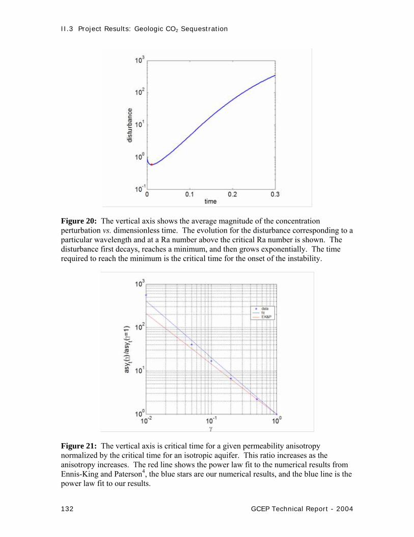
An interesting result of this analysis is that above the critical Rayleigh-Darcy number

all perturbations decay initially before they start growing exponentially as shown in Figure 20. There is an initial period of stability before the onset of the convective movement. The longer this critical time is, the longer it will take until mixing enhances the CO2 dissolution rate. Ennis-King and Paterson observed, and we confirm, that the critical time is a strong function of the permeability anisotropy, as shown in Figure 21. The critical time increases from tens of years to hundreds of years as the anisotropy changes from γ = 1 to γ = 10-2. Even in the worst case this is only a small fraction of the minimum time estimated above to dissolve all CO2 by convective mixing, and therefore only delays it. Finally the stability analysis gives us information about the wavelength λ of the perturbations that grow initially. As for depth greater than the critical depth, the wavelength asymptotically approaches a constant value for a given permeability anisotropy. This wavelength increases with increasing anisotropy; our results show a stronger increase compared with those of Ennis-King and Paterson. The initial wavelength is only an indication of the wavelength established in the fully nonlinear system. A rough estimate for the depth of finger penetration is obtained by setting d = λ/2 in the scaling law for Lf. Using our results λ(γ = 0.1) ≈ 20 m so d ≈ 10 m, and hence the penetration depth of the fingers is roughly on the order of Lf ≈ 200 m ≈ αL. This scaling argument suggests that the instability is strong enough to propagate fingers far enough to mix the dissolved CO2 with a large enough amount of water to dissolve all CO2.



Figure 20: The vertical axis shows the average magnitude of the concentration perturbation vs. dimensionless time. The evolution for the disturbance corresponding to a particular wavelength and at a Ra number above the critical Ra number is shown. The disturbance first decays, reaches a minimum, and then grows exponentially. The time required to reach the minimum is the critical time for the onset of the instability.

Figure 21: The vertical axis is critical time for a given permeability anisotropy normalized by the critical time for an isotropic aquifer. This ratio increases as the anisotropy increases. The red line shows the power law fit to the numerical results from Ennis-King and Paterson4, the blue stars are our numerical results, and the blue line is the power law fit to our results.



The analysis discussed here is based on a flow geometry and a set of simplifying assumptions that may not reflect actual aquifer settings. In a typical aquifer the injected CO2 will flow preferentially through high permeability paths. The interfacial tension between CO2 and brine will be high, and the viscosity of CO2 will be significantly lower than that of brine, so CO2 will displace water inefficiently and vice versa. All of these physical mechanisms will act to increase the volume of brine contacted and the area of contact, which should increase the rate of dissolution. In addition, most aquifers will not be strictly horizontal, and hence there will be some gravity-driven flow in the up-dip direction. This flow will also increase the area of contact. On the other hand, permeability heterogeneity can restrict vertical flow, which would increase dissolution time. Investigation of the interplay of heterogeneity, dissolution, gravity segregation of injected CO2, slow density-driven convection in the brine phase, and diffusion will require high-resolution numerical solutions for the appropriate combination of mechanisms, a task that is next on our agenda. While the streamline approach demonstrated above can handle effectively the injection period, it is not the appropriate choice for examining the interplay of diffusion, convection, and possible chemical reactions that occur in the long term.

Streamline Simulation of CO2 Injection in Saline Aquifers

In the previous section, the convection-enhanced dissolution mechanism for trapping CO2 in an aquifer was discussed. This section focuses on the effect of residual gas trapping on the ability of a given CO2 plume to migrate upwards and potentially leak to formations above the injection zone.

As CO2 is injected into an aquifer, the interplay of various parameters including density and viscosity of brine and CO2 at the prevailing temperature and pressure in the formation will determine the potential for the injected CO2 to migrate upwards in the formation due to buoyancy. Also, the permeability variations within the aquifer and the presence of any potential flow barriers (shales) will play an important role in the trajectory of the injected CO2.

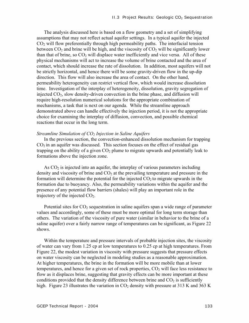
Potential sites for CO2 sequestration in saline aquifers span a wide range of parameter values and accordingly, some of these must be more optimal for long term storage than others. The variation of the viscosity of pure water (similar in behavior to the brine of a saline aquifer) over a fairly narrow range of temperatures can be significant, as Figure 22 shows.

Within the temperature and pressure intervals of probable injection sites, the viscosity of water can vary from 1.25 cp at low temperatures to 0.25 cp at high temperatures. From Figure 22, the modest variation in viscosity with pressure suggests that pressure effects on water viscosity can be neglected in modeling studies as a reasonable approximation. At higher temperatures, the brine in the formation will be more mobile than at lower temperatures, and hence for a given set of rock properties, CO2 will face less resistance to flow as it displaces brine, suggesting that gravity effects can be more important at these conditions provided that the density difference between brine and CO2 is sufficiently high. Figure 23 illustrates the variation in CO2 density with pressure at 313 K and 363 K



(for additional isotherms, see McHardy and Sawan47. If CO2 is injected at supercritical conditions, the density can vary from ~200 kg/m3 at low pressures to ~800 kg/m3 at high pressures. The density of water/brine is a relatively weak function of temperature (~1000 kg/m3 at low temperatures to ~960 kg/m3 at the normal boiling point), and it is a weaker function of pressure. Hence a significant upward driving force due to density differences

Figure 22: Dependence of water viscosity on pressure and temperature46.

Figure 23: Dependence of CO2 density on pressure and temperature.

can exist in warm aquifers, where the mobility of water is high relative to cold aquifers, in which the upward migration of CO2 can be limited by the lower mobility of the brine.

0.0

0.4

0.8

1.2

1.6

2.0

0 5000 10000 15000 20000 25000 30000

Pressure (psia)

Visc

osity

(cp)

32 F

50.5 F

86 F

166.6

0

200

400

600

800

1000

0 100 200 300 400 500

Pressure (atm)

Den

sity

(kg/

m3)

Injection pressure313

363



To estimate the magnitude of gravity-to-viscous forces in a given sequestration setting, we adopt the formulation suggested by Zhou et al.48, who define the ratio of gravity to viscous forces by the dimensionless group, Ngv:

avgv

w

g LKNHvρ

µ∆

= . (15)

In Eq. (1), ∆ρ is the density difference between the injected and the resident fluid, L is the displacement length, Kav is the average absolute permeability in the formation, H is the height of the formation, v is the injection velocity and µw is the viscosity of the initial fluid in the formation (water). To map out the potential range of sequestration scenarios, Table III reports estimates of low and high values of the individual components of Eq. (1) and the corresponding value of the gravity to viscous number Ngv.

Table III: Gravity and viscous forces in aquifer sequestration.

From the reported estimates of high and low values of the gravity to viscous forces, we find that depending on the temperature and pressure of the aquifer (as well as the permeability and injection rates), we might expect to see a full range of flow patterns within the various aquifers from gravity-dominated flow to viscous-dominated flow. In the following subsection, we investigate the effect of changes in fluid properties with temperature and the significance of residual trapping.

To test our qualitative scaling argument, a series of example calculations was performed. All were done with the Stanford compositional streamline simulator, CSLS. The simulator describes the phase behavior of the CO2–brine system by a modified version of the Peng-Robinson equation of state2. Special care must be taken to account properly for the mutual solubility of CO2 and brine. Our approach follows the modifications outlined by Yan et al.49. Temperature-dependent shift parameters are used to ensure accurate prediction of phase densities. Simulation of CO2 injection in the formation shown in Figure 24 was performed at two temperatures to evaluate the impact of variations in fluid properties.

Estimate ∆ρ (kg/m3)

L (m)

H (m)

Kav (mD)

v (m/day)

µw (cp)

Ngv

High 800 1E5 200 1000 10 1 33.5 Low 200 1E3 10 1 0.1 0.2 0.84



Figure 24: Permeability field used in simulation study. The formation is a 6000 m by 189 m cross-sectional area of an aquifer consisting of 5

high-permeability (3000 mD) sand compartments separated by low-permeability shales (3 mD). The porosity of the sands is 35% whereas the porosity in the shales is 3.5%. The simulation grid is 100*62, a bit on the coarse side, but sufficient to investigate variation in flow patterns with temperature. Corey type relative permeability curves were used with an irreducible brine saturation of 0.2. The same relative permeability cures were used for the sandstones and shales. The first example simulation was performed at 313 K (40C). The sequestration process was simulated for two years for four values of the critical gas saturation (0, 0.05, 0.1 and 0.2). Figure 25 reports the fluid distribution at the end of the injection phase.

As the residual gas saturation is gradually increased, the tendency for the CO2 to follow the preferential flow paths below the shales decreases. Also, the significance of the gravity override decreases as gas is trapped with increasing Sgc. From Figure 25, it is clear that the critical gas saturation can play an important role in preventing the free CO2 from migrating to the top of the formation. Comparison of the locations of the gas fronts in the top (Sgc = 0) and bottom panels (Sgc = 0.2) of Figure 24 indicates that the increase in Sgc must result in an increase in the amount of CO2 that is dissolved in the brine. Figure 26 reports the concentration maps for two of the displacements illustrated in Figure 25. It confirms the observation that although a smaller volume of the brine is contacted by CO2 at high Sgc, the concentration of CO2 in the contacted brine is higher than for Sgc = 0. For comparison with the second set of displacement calculations, we note that the ratio of gravity to viscous forces for the low temperature displacements is estimated to Ngv = 4.1.

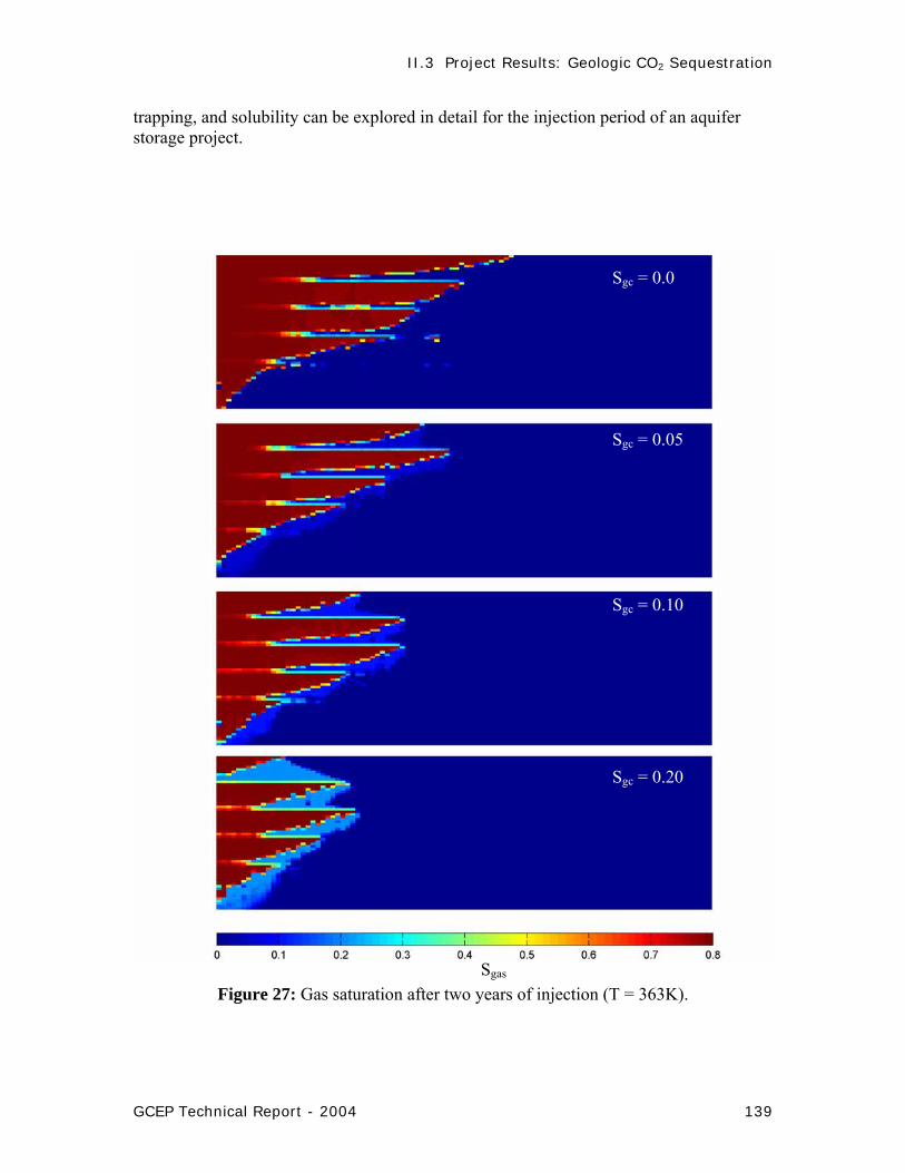
In the second set of displacement calculations, the temperature of the aquifer was set to 363K (90C). Accordingly, the viscosity of the brine is reduced from ~0.653 cp to ~0.276 cp, while the viscosity of CO2 declined from 0.05 to 0.025 cp. In this displacement the gravity-to-viscous ratio was Ngv = 21.1. Figure 27 demonstrates that there is a more significant impact of gravity segregation at the higher temperature. As for the low temperature calculations, the sequestration process was repeated for four levels of

log(K)



Figure 25: Gas saturation after two years of injection (T = 313K).

Sgc = 0.05

Sgc = 0.0

Sgc = 0.10

Sgc = 0.20

Sgas



Figure 26: Mole fraction of CO2 dissolved in the brine (T = 313K) critical gas saturations, Sgc (0, 0.05 0.1 and 0.2). The results of the simulations after two years of injection are reported in Figure 27. For the high temperature (high mobility of brine) we find a significant increase in the predicted gravity override. Four factors contribute to the increase in gravity segregation: (a) the gas phase is less restricted to flow in the vertical as well as the horizontal direction due to the decrease in brine viscosity, (b) the density difference between the injected CO2 and the brine has increased as the CO2 now has a density of ~260 kg/m3 as opposed to the low temperature displacement where the injected CO2 had high density of ~670 kg/m3, (c) at the higher temperature, the solubility of CO2 in the brine is lower resulting in a larger volume of mobile low-density gas in the formation, and (d) the ratio of water viscosity to CO2 viscosity increases at the higher temperature, resulting in a lower local displacement efficiency.

The simple scaling arguments and examples presented here, demonstrate the impact of the fluid properties in an aquifer injection process on the tendency of the injected CO2 to migrate upwards in the formation. The examples also confirm the utility of the streamline simulation approach for this problem. Numerical solutions were used along streamlines, which were updated periodically, as gravity segregation shifted streamlines. Each simulation took about ten minutes of computation time. Those simulations can be performed at low enough cost in computation time that the interplay of heterogeneity,

xCO2.

Sgc = 0.2

Sgc = 0.0



trapping, and solubility can be explored in detail for the injection period of an aquifer storage project.

Figure 27: Gas saturation after two years of injection (T = 363K).

Sgc = 0.05

Sgc = 0.0

Sgc = 0.10

Sgc = 0.20

Sgas



Time Scales for Coalbed Sequestration Enhanced coal bed methane (ECBM) recovery combined with CO2 storage is one

option for sequestration of CO2. Flow through coalbed reservoirs occurs in a network of subparallel face cleats orthogonally intersected by butt cleats. For a mature, high-rank coal, typical cleat aperture is approximately 0.1 mm, and typical cleat spacing is 1-2 cm50,51. When CO2 is injected, it flows through the cleat system and diffuses into the matrix. Preferential adsorption of CO2 causes adsorbed CH4 to desorb. The desorbed CH4 then diffuses through the matrix to the cleat system, where it flows to the production well and is produced. Diffusion through the matrix is controlled by concentration gradients, while flow through the cleat system is controlled by pressure gradients. The rate of production from coalbed reservoirs is controlled by the slower of these two processes. In this section, we consider the question of whether it is appropriate to model field-scale flow in a coalbed with an assumption of local chemical equilibrium between coal and gas or whether some more complex model is required.

The following simple scaling analysis examines the effect of diffusion transport in the cleat and matrix systems. In cases where convection dominates, the local equilibrium assumption is reasonable. If the local equilibrium assumption can be made, then the cleat network controls flow through coal bed reservoirs, and the details of matrix diffusion effects need not be represented explicitly. Cleat System. Flow in the cleat system can be described by the convection-dispersion equation shown in Eq. 16, which describes the concentration of injected gas in the fracture system, Cf. The Peclet number (Pe), defined in Eq. 17, is a ratio of the characteristic time for diffusion to the characteristic time for convection.

21 0ff f

CC C

Peτ∂

+ ∇ ⋅ − ∇ =∂

, (16)

where

f

f

vLPe

D= , (17)

and τ is dimensionless time, v is the average flow velocity in the fractures, Lf is the displacement length, and Df is the diffusion coefficient in the gas phase in the fractures. Large values of Pe characterize convection-dominated flows. For typical ECBM displacements, Pe is very large. For a flow velocity of 0.33 m/d, a flow length of 400 m, and a diffusion coefficient in the gas of 10-4 cm2/s, for example, the resulting Peclet number is 1.5 x 105. That value is large enough that it is quite reasonable to neglect the effects of longitudinal diffusion in the flow calculation. Matrix System. In the coal matrix system, we assume that diffusion is the only mechanism of transport. The conservation equation is

mm m

C D Ct

∂= ∇ ⋅ ∇

∂, (18)



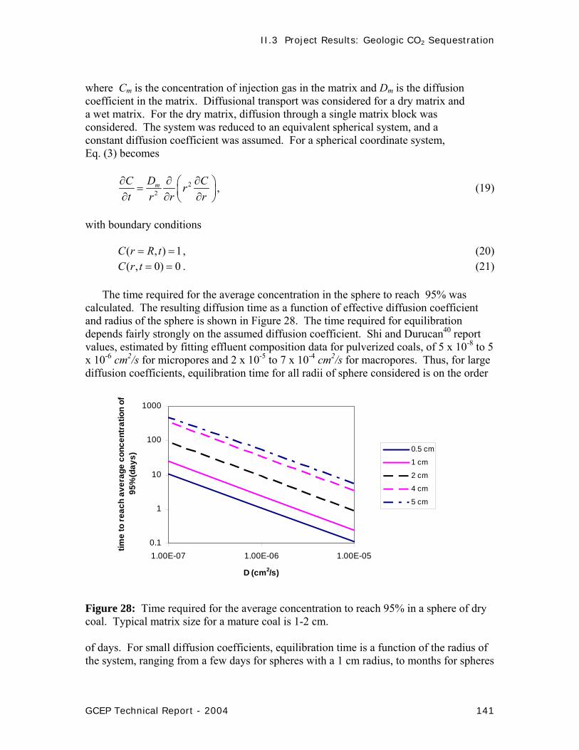
where Cm is the concentration of injection gas in the matrix and Dm is the diffusion coefficient in the matrix. Diffusional transport was considered for a dry matrix and a wet matrix. For the dry matrix, diffusion through a single matrix block was considered. The system was reduced to an equivalent spherical system, and a constant diffusion coefficient was assumed. For a spherical coordinate system, Eq. (3) becomes

22mDC Cr

t r r r∂ ∂ ∂⎛ ⎞= ⎜ ⎟∂ ∂ ∂⎝ ⎠

, (19)

with boundary conditions

( , ) 1C r R t= = , (20) ( , 0) 0C r t = = . (21)

The time required for the average concentration in the sphere to reach 95% was

calculated. The resulting diffusion time as a function of effective diffusion coefficient and radius of the sphere is shown in Figure 28. The time required for equilibration depends fairly strongly on the assumed diffusion coefficient. Shi and Durucan40 report values, estimated by fitting effluent composition data for pulverized coals, of 5 x 10-8 to 5 x 10-6 cm2/s for micropores and 2 x 10-5 to 7 x 10-4 cm2/s for macropores. Thus, for large diffusion coefficients, equilibration time for all radii of sphere considered is on the order

Figure 28: Time required for the average concentration to reach 95% in a sphere of dry coal. Typical matrix size for a mature coal is 1-2 cm. of days. For small diffusion coefficients, equilibration time is a function of the radius of the system, ranging from a few days for spheres with a 1 cm radius, to months for spheres

0.1

1

10

100

1000

1.00E-07 1.00E-06 1.00E-05

D (cm2/s)

time

to re

ach

aver

age

conc

entr

atio

n of

95

%(d

ays)

0.5 cm

1 cm

2 cm

4 cm

5 cm



with a 5-cm radius. For a high rank coal, where fracture spacings are small, equilibration time is on the order of tens of days for a typical solid diffusion coefficient of 10-7 cm2/s.

Coal reservoirs are typically water saturated, and the coal surface is water wet53. In

this system, for mass transfer between matrix and fracture systems, we assume that gas must diffuse through a thin film of water. The presence of water creates extra resistance to mass transfer. The concentration gradient driving mass transfer in the water phase is relatively low, because the solubility of gas in the water limits the concentration gradient in that phase.

Figure 29: Schematic of a simplified wet matrix system.

For this calculation, the wet matrix was approximated as a spherical film of constant thickness, surrounding the matrix (Figure 29). The time to reach the 99% of the solubility concentration at ra is presented as a function of diffusion coefficient and film thickness in Figure 30. For the range of thicknesses and diffusion coefficients considered, film equilibration times are very short (on the order of minutes) compared to matrix equilibration times. Diffusion coefficients for CO2 in water at high pressure are on the order of 10-5 cm2/s52. Hence we conclude that for a typical cleat aperture of 0.1 mm, the time required for diffusion through a water film with similar thickness is small compared to the other characteristic times for flow and equilibration.

This simple analysis of diffusion in the cleat and matrix system suggests that

diffusion times are short enough that for flow at field scale, it is a reasonable approximation to assume that the fluid in the cleat system is in equilibrium with the solid. If so, then the problem of representing adsorption of CO2 and other gases in a coalbed revolves around accurate representation of the multicomponent adsorption. If a suitable model of that adsorption is available, it should be possible to take advantage of the speed of streamline simulation techniques for this system.

R

ra



0.01

0.1

1

10

100

1.00E-06 1.00E-05 1.00E-04

D (cm2/s)

t (m

inut

es) 0.1 cm

0.075 cm0.05 cm0.025 cm0.01 cm

Figure 30: Time required for wet film to reach solubility concentration.

Enhanced Coalbed Methane Recovery and CO2 Sequestration The relatively advanced state of knowledge regarding the mechanisms of EOR is not

matched for gas injection into coalbeds. Our previous analytical study of the flow of multicomponent gases through dry coal (Zhu et al.8) revealed the strong coupling between the advance of a gas species and its adsorption properties. It was predicted that coals are capable of separating CO2 from N2, among other results. Experimental verification of model predictions appears prudent before adding more detail to the calculations.

An experimental program was begun with the goals of validating prior flow and

adsorption predictions as well as developing a database for comparison of more advanced predictions. The apparatus developed is illustrated in Figure 31. The centerpiece is the core holder for holding coal samples that are 4.25 cm in diameter and up to 25 cm long. To date, we have employed crushed (60 mesh) and dried coal samples from the Powder River Basin. The crushed coal is packed to obtain a porous medium with a permeability of 80-100 md and a porosity of 0.33 The apparatus is capable of using intact core samples, but no field samples available to us had sufficient integrity to be employed directly.



To vent Gas analyzer

Gas flowmeter Gas flowcontrol meter

PC

Vacuum pump

To vent

Electronic balance

Coal holder

Gas cylinder

Pressure transducer

valve

Figure 31: Schematic of experimental apparatus.

Coal surfaces are equilibrated with methane at a given pressure, typically between 500 and 750 psi. The displacement gas is a mixture of CO2 and N2, and its flow is metered by a 0-50 SCCM (standard cubic centimeters per minute) mass flow controller. The concentration of gas components (CO2, CH4, N2) in the effluent and at sampling ports along the length of the core is measured with a gas analyzer to ±0.01%. The rate of gas production is also measured as is pressure drop along the core. A backpressure regulator maintains the outlet of the system at constant pressure.

A first step in the investigation was the measurement of the adsorption and desorption

properties of pure CO2, CH4, and N2 on the coal. Measurement results are given in Figure 32. Several notes are in order. First, CO2 was the most strongly adsorbing gas. At 800 psi, roughly 3 times as much CO2 adsorbed as did CH4 and more than 8 times as much CO2 adsorbed as did N2. Second, there was significant hysteresis among adsorption and desorption results. Upon depressurization, coal retained significant volumes of gas. At 220 psi, this coal retained 80% of the CO2 that had adsorbed at 800 psi. The hysteresis between adsorption and desorption characteristics does not yet have a satisfactory physical explanation. Nevertheless, the difficulty in desorption of CO2 suggests that coal may be a secure site for CO2 sequestration.



0

200

400

600

800

1000

1200

1400

1600

1800

0 200 400 600 800 1000 1200

Pressure, psig

Ads

orpt

ion,

SC

F/to

n

CO2 adsorptionCO2 desorptionCH4 adsorptionCH4 desorptionN2 adsorptionN2 desorption

T=22°C

CO2

CH4

N2

Figure 32: Adsorption-desorption isotherm for gases on crushed, dried samples of Powder River Basin, WY coal at 22°C.

A suite of displacement experiments is underway to be used subsequently to interpret

ECBM and sequestration mechanisms and thereby to provide a first step in improving conceptual and mathematical models. Some representative results follow. Figure 33 provides a comparison between pure N2 and CO2 as injection gases. The figure shows the composition of gas exiting the coal versus the amount of gas injected in pore volumes (PV) computed at the outlet pressure of the coal. Comparison of Figures 33(a) and (b) shows that injected N2 broke through to the exit in about 0.4 PV whereas CO2 did not appear until after 1.5 PV of total gas had been injected. Note also that a significant fraction of the CH4 produced as a result of N2 injection was mixed with N2. About 3 PV of total injection was required to sweep out the CH4 with N2. Production of CH4 as a result of CO2 injection was virtually complete when CO2 broke through at 1.5 PV, and there was little production of CH4/CO2 mixtures. Permeability of the pack decreased by 34% as CO2 replaced CH4. Total recovery of the initial CH4 in the system was 77% with N2 injection and 92% as a result of CO2 injection. With respect to recovery, breakthrough time, and the mixing of injection gas and CH4, CO2 is the superior injection gas.

Injection gases with various concentrations of CO2 and N2 have also been tested.

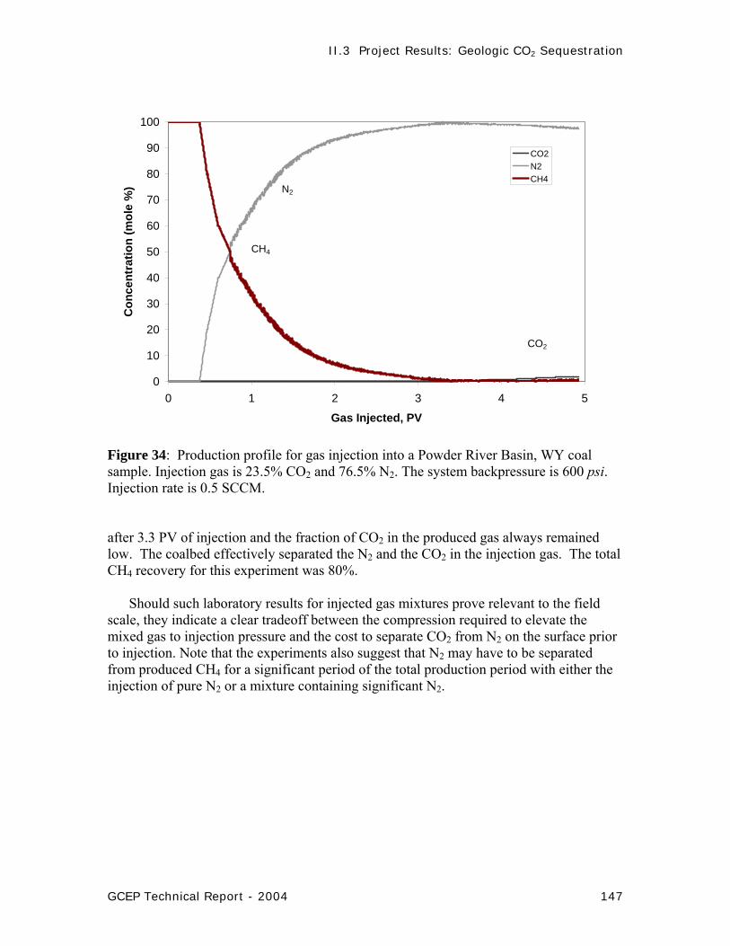
Figure 34 shows the production profiles resulting from an injection gas with 23.5% CO2 and the balance N2. Such a mixture might be similar to a combustion gas enriched in CO2 but not separated completely. Notably, N2 broke through at the outlet in roughly 0.4 PV, and its concentration increased rapidly thereafter; however, CO2 did not appear until



0

10

20

30

40

50

60

70

80

90

100

0 1 2 3 4 5

Gas Injected, PV

Con

cent

ratio

n (m

ole%

)

CH4N2

N2

CH4

(a)

0

10

20

30

40

50

60

70

80

90

100

0 1 2 3 4 5Gas injected, PV

Con

cent

ratio

n, m

ole

%

CO2CH4

CH4

CO2

(b)

Figure 33: Production profiles for pure gas injection into a Power River Basin, WY coal sample: (a) pure N2 injection gas and (b) pure CO2 injection gas. The system backpressure is 600 psi. Injection rate is 0.5 SCCM.



0

10

20

30

40

50

60

70

80

90

100

0 1 2 3 4 5

Gas Injected, PV

Con

cent

ratio

n (m

ole

%)

CO2N2CH4

N2

CH4

CO2

Figure 34: Production profile for gas injection into a Powder River Basin, WY coal sample. Injection gas is 23.5% CO2 and 76.5% N2. The system backpressure is 600 psi. Injection rate is 0.5 SCCM. after 3.3 PV of injection and the fraction of CO2 in the produced gas always remained low. The coalbed effectively separated the N2 and the CO2 in the injection gas. The total CH4 recovery for this experiment was 80%.

Should such laboratory results for injected gas mixtures prove relevant to the field scale, they indicate a clear tradeoff between the compression required to elevate the mixed gas to injection pressure and the cost to separate CO2 from N2 on the surface prior to injection. Note that the experiments also suggest that N2 may have to be separated from produced CH4 for a significant period of the total production period with either the injection of pure N2 or a mixture containing significant N2.

ii.3.2 rapid prediction of co2 movement in aquifers, coal ... · ii.3.2 rapid prediction of co2...

Documents