ii background information - puc-rio
TRANSCRIPT

IIBackground Information
In this chapter, we will discuss some related concepts with large data
management solutions. Section II.1 will briefly describe the cloud computing
concept, and its characteristics. In section II.2, we will explain how cloud
computing is being used to support large scale data management when
handling a single large application’s data or when handling many applications’
data. Then, section II.3 introduces the MapReduce programming model,
and its distributed file system. Section II.4 describes high-level programming
languages made on top of MapReduce, and how they are related to this work.
Section II.5 explicates the different types of joins implemented by the Pig
framework, and finally section II.6 describes some of the statistical techniques
that have been used for performance prediction.
II.1 Cloud Computing
Cloud computing has gained a large amount of interest in the IT industry
as well as in academia. As a result, the market for cloud computing services
is expected grow up to $42bn/year by 2012 [42]. On the other hand, there are
several research works that study the challenges posed by cloud computing
(e.g. [7, 12, 83], among others). Nevertheless, the majority of these works have
mostly focused on studying general technical challenges and little (or none)
work has been done on gathering all works on a specific research area.
Cloud computing has not yet an standarized concept, but there are
many proposals in the literature e.g. [104, 110]. In spite of that, the definition
provided by the US National Institute of Standards and Technology (NIST)
appears to be the one that captures the agreed aspects of cloud computing [84].
The concept addresses aspects such as:
– Cloud computing characteristics: On-demand self-service, Broad network
access, Resource pooling, Rapid elasticity, and Measured service.
– Deployment models: Private clouds, Community clouds, Public clouds,
and Hybrid clouds.

Chapter II. Background Information 12
– Service models: Software as a Service, Platform as a Service, and Infras-
tructure as a Service.
Cloud computing popularity is making many applications to move to
the cloud. This is mainly motivated by its two most appealing features, the
elastic nature of resources and the pay-as-you-go model. These applications
require systems capable of providing scalable and consistent data management
as a service in the cloud. The new settings imposed by cloud computing
can make traditional database deployments become scalability bottlenecks
and, therefore, this would limit cloud benefits. This is due to the dificulty of
making traditional databases suitable for large scale deployments, or for elastic
deployements (to have the ability of using new nodes whenever is needed, and
stop using them when they are not longer needed).
II.2 Cloud Data Management
There are different scalable data management solutions which can take
advantage of cloud features and become more attractive when deployed in
such environments. Most traditional relational database systems were not
originally designed to take advantage of characteristics such as elasticity, high-
availability, self-manageability, or the ability to run on commodity hardware.
Different types of applications have appeared using clever deployments in order
to guarantee some cloud features, and they can be classified by the amount of
data handled. In the following sections, we will describe some applications that
handle big data II.2(a), and other approaches that manage a large number of
small applications II.2(b).
(a) Big data
This type of applications focus in building large data storage systems that
deal with various applications. Most of the time start small, but due to the
internet, these applications evolve and so does their data. As they evolve, their
data management requirements change, and sometimes these new requirements
can or can not be managed by traditional relational database. In addition to
this, most RDBMSs have not been able to incorporate cloud features which
make them less attractive for the deployment of large scale applications in
cloud environments.
In this manner, different data stores have been designed to fulfill these
large scale requirements and to support cloud features. For example, there
are two important large-scale data management systems that have provided
many new ideas to the database community, Bigtable [20] and Dynamo [25].

13 II.2. Cloud Data Management
The former is presented as ”a distributed storage system for managing struc-
tured data, designed to scale to petabytes of data on thousands of commodity
servers”. Besides, it provides to its clients the ability to dynamically control
whether to take the data out of memory or from disk by using system param-
eters. It is worth noting that Bigtable’s data is horizontally and dynamically
partitioned using tables’ row ranges. Each row range is called a tablet, and is
the distribution and load balancing unit of Bigtable.
On the other hand, Dynamo [25] is presented as a highly available
key-value storage system to help Amazon’s services provide an ”always-on
experience”. This means that high-availability is one of the most important
requirements in its design due to the fact that a minimal outage would cause
huge economic consequences and would also have a big impact on customer’s
trust. Dynamo stores small binary objects (up to 1MB) with unique IDs
where no operation can affect multiple data items. For partitioning its data,
it uses a consistent hashing method similar to Chord’s scheme [100]. This
design decision gives Dynamo the advantage of incremental scalability because
a node can be scaled without causing negative impact to the system. To
achieve high-levels of availability, Dynamo sacrifices ACID consistency and
provides only eventual consistency. This means that multiple versions of the
same object might co-exist. Eventual consistency implies the extensive use of
object versioning and the possibility of requiring application-assisted conflict
resolution (i.e. semantic reconciliation) if the system cannot resolve conflicts
automatically (i.e. syntactic reconciliation).
These two works boosted the development of some open-source projects
such as Voldemort [8], Dynomite [9], Cassandra [76], among others that
were modeled after Dynamo’s architecture, and systems like HBase [101] and
Hypertable [67] that follow Bigtable’s implementation.
(b) Large small data
Cloud data management also aims to support a large number of appli-
cations but all having a small amount of data. This type of applications could
be solved using large multitenant systems [5] i.e. a single software deployment
serving multiple clients. This produces savings on software deployment, but
adds complexity to manage many applications.
There are interesting approaches which involve open-source software, and
cloud infrastructure deployment to deal with this type of applications using
cloud strategies. For instance, the works presented by Yang et al. in [108], and
the one presented by Hui et al. [58] are complementary in an orthogonal way.
This is because [108] describes the infrastructure needed for a scalable data

Chapter II. Background Information 14
platform that deals with a large number of small applications. In addition to
this, a suitable data model for deploying a multi-tenancy database management
system is described by [58].
Even though these two works show different approaches to alleviate the
scalability and cost problems, the adopted strategies are similar to other cloud
data management solutions. For example, the major difference between the
architecture deployment explained in [108] and the one explain in [6] is the
way in which fail-over is performed (client driven versus application driven).
On the other hand, the work in [58] presents a specific data model for storing
multi-tenancy data, and the indexing techniques explained are also similar
in spirit to the work presented in [74] because both aim to provide index
information in the form of a distributed index served to an arbitrarily large
number of concurrent users.
II.3 The Map Reduce programming model
(a) Map Reduce
In order to take advantage of the ”infinite” resource supply offered by
the clouda, specific parallel query languages were needed. A very important
contribution in this topic is the programming model MapReduce [24] which
has become almost a de facto standard for massive dataset computations in
the cloud. It is a programming model but it is associated to an implementation
for processing and generating large datasets developed at Google [24].
The large amount of data that has to be daily processed at Google
was their main motivation. Most tasks were relatively simple but due to the
scale of the problem, these simple tasks became complex. Take the case of
finding the number of queries submitted to Google’s search engine any day
by any user. This task could probably be solved using a simple SQL query.
But if the input to this task is so large that it is stored in a distributed way,
the scenario would change as well as the solution to be applied. It would
require distributed processing over hundreds of computers of a specialized
cluster in order to get the results in an acceptable query response time. The
distributed processing of the simple task would usually add more complexity
to the problems because programmers had also to take care of distributing,
partitioning and parallelizing the computation i.e. they could not focus on the
actual simple computation without worrying on how to do it in a scalable way.
Thus, Dean et. al. [24] created such an abstraction in order to facilitate
coding in a distributed way to programmers. The MapReduce framework

15 II.3. The Map Reduce programming model
Figure II.1: The MapReduce Model [106]
proposed by the authors provides characteristics such as fault tolerance, load
balancing, and task parallelization in a transparent way. The MapReduce
computing model requires the users to specify two functions: a map function
which processes structured or unstructured data in a key/value fashion, and
then generates a set of intermediate key/value pairs. It also requires a reduce
function which will match all the data with each possible intermediate key
generated in the map phase, and perform aggregations over the data records
with the same key generated in the map phase.
The figure II.1 shows graphically how the MapReduce model works. The
underlying framework is in charge of splitting the data among parallel map
tasks considering data locality. This is how the framework manages to take
the computation towards the data which is cheaper than the moving the data
around. In the figure, each part of the data called split will be assigned to a
map task. Then, the map tasks will output the result of their computations in
a key-value form which will be sent across the network to the corresponding
reduce tasks. Between the map and the reduce phases of the execution the
intermediate map data is shuffled across the reduce nodes and a distributed
sort is performed. In this way, all the values with the same key will be sent
to the same reduce node which will usually perform computations over them.
Finally, the reducers will output the result of the whole process.
There are many implementations of the MapReduce distributed comput-
ing paradigm. The one used the most is the open source framework Hadoop [30]
which was created to support a search engine initiative, called Nutch [35].
Later, it was taken by Yahoo! to address a critical business need i.e. to man-

Chapter II. Background Information 16
age its exponentially increasing volumes of data. This implementation is used
in many other open source projects because of its ability to process data in
a distributed way while using commodity hardware. The Hadoop framework
consists of two main services: the JobTracker, which coordinates the work and
the TaskTrackers that perform the computation locally at each node.
While the original MapReduce framework was implemented in C++,
there are many implementations in specific programming languages. For ex-
ample, there are implementations in Ruby [93], Haskell [11, 96], Java [30],
Python [17], C# [87], among other programming languages. In addition, there
exist variations of the framework such as a file-based and not tuple-based im-
plementation [29] or an implementation for shared-memory multi-cores and
multiprocessors systems [109]. At the same time, there are domain specific
implementations such as for mobile applications [26], or the for graphics pro-
cessors [47].
(b) Distributed file system
To take full advantage of the distributed computation, the original
MapReduce implementation uses an underlying distributed file system, Google
File System (GFS) [41], in order to access the data in a local manner. GFS has
a master/slave architecture consisting of a Master node and a large number
of working nodes. All the files stored in the GFS are broken up into fixed size
chunks of about 64MB in order to have a better performance in I/O operations
due to size similarity with sectors in regular file systems. These file chunks are
then stored and distributed along all the working nodes, called Chunk servers,
available while the metadata associated with all of them is kept in the Master
node.
There is also an open-source implementation of GFS that works
along with the Hadoop framework called Hadoop Distributed File System
(HDFS) [33]. It is a fault tolerant distributed file system designed to run on
large commodity clusters on which storage hardware is attached to the com-
pute nodes. HDFS employs a master-slave architecture where the master, the
Namenode, manages the file system namespace and access permissions i.e. the
metadata of the system. In addition to that, all slaves, the Datanodes, manage
the storage attached to the physical nodes on which they run.
All files stored in the HDFS are split into a number of blocks which are
replicated and stored on the datanodes for enforcing high-availability of the
system. The information about the location of each file block is managed by
the Namenode. Each data block is identified by a Block ID that represents
its position in the file and a unique, monotonically increasing generation

17 II.4. High level computing languages for data intensive applications
Figure II.2: Hadoop Computing Model
timestamp. These IDs are assigned by the Namenode in order to guarantee
that there are not two HDFS blocks with the same Generation Timestamp [3].
Figure II.2 outlines how HDFS works along with Hadoop. The Datanodes
usually reside in separate nodes to take advantage of not having to share
storage with other processes. That is why the Map processes are sent into
Datanodes which contain the file blocks needed. Job executions are monitored
by the JobTracker which usually resides in a separate node from the working
nodes (TaskTrackers or Datanodes). The Namenode is most of the time in
the same node as the JobTracker because they are just two processes that do
not consume as many resources as the other framework processes. These two
processes are in charge of monitoring how the data processing works, and the
distribution of the data along the nodes.
II.4 High level computing languages for data
intensive applications
An important drawback of the MapReduce framework is that network
latency and file replication used determine the performance and availability of
the system. An important work is [92] where the operations described in the
original MapReduce paper were tested against regular database systems, and
also against parallel databases. Even though the data operations performed
on both systems were the same, a conclusion drawn from this paper is that
MapReduce and databases target different data management tasks.
MapReduce can be improved in many different ways such as providing
new access methods, file replication levels, usability, among other existing
features in databases. That is why systems such as Sawzall [43], Pig-Latin [90],
DryadLINQ [111], SCOPE [18] and HIVE [102] have been built resembling

Chapter II. Background Information 18
this new computing paradigm. For instance, Google’s Sawzall is a high level
programming language that facilitates users to perform massively parallel
processing across large clusters by abstracting the MapReduce programming
model. Similar to original MapReduce framework, Sawzall’s syntax is very
similar to C and Pascal statements. In the same way, DryadLINQ and SCOPE
are extensions of the Dryad system [69] (a distributed execution engine similar
to MapReduce developed by Microsoft Research).
In the open source world, Yahoo!’s Pig and Facebook’s HIVE are
important projects. HIVE uses a subgroup of the ANSI SQL-92 standard with
some extra features called HiveQL. This scripting language is able to work
in a distributed manner because HIVE compiles its HiveQL statements into
MapReduce jobs, and then executes them in a computer cluster.
Pig is an abstraction layer of the Hadoop framework which compiles data
analysis tasks into Map-Reduce jobs and executes them on Hadoop. But the
Pig framework uses a language for expressing dataflows called Pig-Latin. One
of Pig-Latin’s biggest advantages is that it enables programmers to express
data transformation tasks in a few lines. Pig-Latin also differs from SQL in
which the former allows expressing transformations as a sequence of steps,
and the latter describes desired outcome. This is seen as another advantage
because writing a sequence of steps comes natural to developers and allows
them to write more complex data flows.
For example, let’s suppose that we have some logs that contain users’
information about accesing a website. These logs would contain user’s id, the
region from the query has been done, and the query itself. Now consider that
we want to obtain the number of queries performed in all regions. If we would
solve this using a SQL query, then we would do it in the following way: We
would first filter the data, then apply a user-defined function called ’Clean’.
And finally, we would count the number of remaining entries in the log for
region.
SELECT U.regions, count(*) as total
FROM UsersRegistry U
WHERE Clean(U.query) = 10
GROUP BY U.regions
In Pig-Latin, this example could be written as:
user_registry = LOAD ’UsersRegistry.dat’
AS (userId, userRegions, userQuery);
users_filtered = FILTER user_registry BY Clean(userQuery);
users_grous = GROUP users_filtered BY userRegions;

19 II.5. Join types in the PIG framework
output = FOREACH users_grous
GENERATE $0 AS regions, count($1) as total;
STORE output INTO ’results.txt’ USING PigStorage();
These works show that high level programming languages for program-
ming large-scale parallel computations are going to be more predominant than
plain MapReduce or other type of distributed jobs. They also outline that fur-
ther improvements need to be made to MapReduce programming models such
as a better use of input files, its lack of schema support or make them more
self-manageable.
II.5 Join types in the PIG framework
The join operation consists in getting all combinations of tuples in both
datasets that are equal on their common attribute names. The idea of relating
datasets makes this operation one of the workhorses of data processing, and
an operation that is likely to be present in most data processing tasks.
The Pig Framework has also the join operation implemented, and it is
likely to be present on the majority of Pig-Latin scripts. It has four different
join algorithms: Hash join, fragment-replicated join, merge join, and skew joins.
Each type is sometimes more suitable for different types of operations, or
different data distributions. We will work with the first three join operators
because the last one directly depends on data distribution i.e. it is applied
only when the underlying data has a skew distribution. Then, we would have
to know a priori the data distribution which is not possible most of the time,
specially when working with large amounts of data because we would have to
pre-process the data to obtain this type of information. That is why we decided
to focus on the most used join operators.
(a) Hash Join
This is the default join operator in the Pig framework. The main idea of
this join is to use keys for each input. Then, when those keys are the same, the
two records will be joined, and the records that did not fulfill the condition
are dropped.
In this way, Pig implements this strategy by tagging each record with
the input which it came from in the map phase, and using the join key as the
shuffle key. This type of join needs a reduce phase where all the records with the
same value for the join key are collected together, and then it performs a cross
product between the records from both inputs. Pig tries to minimize memory
usage by making the records of the first input arrive first and store them into

Chapter II. Background Information 20
Figure II.3: MapReduce Hash Join
cache, so when the records of the second input arrive, they can be probed
against each record from the first input to produce an output record [39].
Figure II.5(a) shows how this process is done. In the map phase, all
records are tagged with the input which they came from, and the cross product
is done in this phase as well. But only the records which keys are the same are
the ones sent through the network. This is done to avoid data transmission
overhead because network resources are the most expensive. The records sent
through the network use as key the attribute used for joining. For example,
the records {1 - 0 - Joe}, and {1 - 1 - Lima} are both using the number 1 as
their key. The second values, 0 and 1, are tags from the input they come from.
So in the reduce phase, these records are merged together, and output as the
result.
An important feature of the hash join is that when using a multi-way
join all the inputs, except the last one, will be held in memory. So, the last
input can be streamed through. In this way, it is a good practice to place at
last the input with more records per given value of the key. Thus, there will
be a better memory usage and the Pig script’s performance can be improved.
The code below shows how this type of join is implemented in a Pig-Latin
script. The example shows the sequence of steps to be done to perform a join
between two relations, inventory and item. The first line shows how to load the
”inventory.dat” file from the ”pigData” folder and using the ’|’ character as
column delimiter. The second line shows the same loading operation, but for
the ”item.dat” relation. And the third line shows the join operation between
both relations. The hash join operation is used as default for joining datasets
in the Pig system, that is why it does not have to be specified on the join

21 II.5. Join types in the PIG framework
command.
--hash.join.pig
user = LOAD ’pigData/user.dat’ using PigStorage(’|’) AS
(i_region_sk:int, user_name:chararray);
region = LOAD ’pigData/region.dat’ using PigStorage(’|’) AS
(i_region_sk:int, region_name:chararray);
join_user_region = JOIN user BY i_region_sk, region BY i_region_sk;
The Pig framework also supports outer-joins by using the hash join
operator, but only when the schema is known. So if we were going perform
an outer-join, Pig can fill in nulls for the side needed i.e. for left outer joins,
the schema of the right side must be provided, and for right outer joins, the
schema of the left side must be provided. This is similar to how outer-joins work
in SQL. Thus, when inner joins are performed, all records with null values are
ignored, and when outer joins are executed, those records are kept, but they
will not match any records.
(b) Fragment-Replicated Join
A routine task is to perform lookups using a small input i.e. looking for
values that are determined on a small input in a larger dataset. For example,
if we would have to process all the sales for a long period of time where we
have sales information with the item’s codes sold. But if we want to use item’s
description instead of item’s code number, it would be easier to load all of our
items into memory and then translate item’s codes into their descriptions. This
is because we have less items than the total number of sales. In this type of
situations, we could avoid the reduce phase used in the hash join operator by
sending the smaller relation to every working node, loading it into memory, and
then performing the join locally without copying data through the network.
This join strategy is called fragment-replicate join because we fragment
one file (the bigger file will be fragmented and their parts will be processed by
the mappers), and replicate the other one (the smaller file will be replicated
to all the mappers).
In order to implement this join strategy, Pig takes advantage of a tool
provided by the Hadoop framework, the distributed cache. This tool enables
us to send a file to the working nodes, and pre-load it onto the local disks,
so the mappers or reducers can access it if needed. The main advantage of
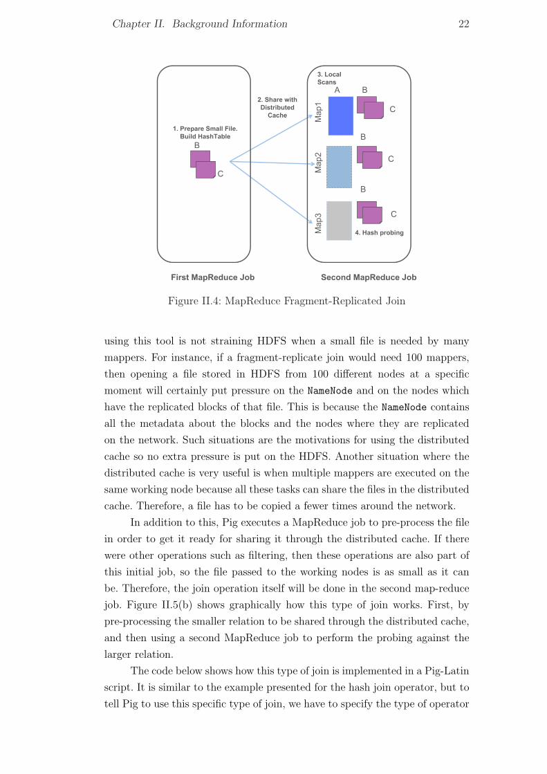
Chapter II. Background Information 22
Figure II.4: MapReduce Fragment-Replicated Join
using this tool is not straining HDFS when a small file is needed by many
mappers. For instance, if a fragment-replicate join would need 100 mappers,
then opening a file stored in HDFS from 100 different nodes at a specific
moment will certainly put pressure on the NameNode and on the nodes which
have the replicated blocks of that file. This is because the NameNode contains
all the metadata about the blocks and the nodes where they are replicated
on the network. Such situations are the motivations for using the distributed
cache so no extra pressure is put on the HDFS. Another situation where the
distributed cache is very useful is when multiple mappers are executed on the
same working node because all these tasks can share the files in the distributed
cache. Therefore, a file has to be copied a fewer times around the network.
In addition to this, Pig executes a MapReduce job to pre-process the file
in order to get it ready for sharing it through the distributed cache. If there
were other operations such as filtering, then these operations are also part of
this initial job, so the file passed to the working nodes is as small as it can
be. Therefore, the join operation itself will be done in the second map-reduce
job. Figure II.5(b) shows graphically how this type of join works. First, by
pre-processing the smaller relation to be shared through the distributed cache,
and then using a second MapReduce job to perform the probing against the
larger relation.
The code below shows how this type of join is implemented in a Pig-Latin
script. It is similar to the example presented for the hash join operator, but to
tell Pig to use this specific type of join, we have to specify the type of operator

23 II.5. Join types in the PIG framework
to use. We accomplish this by adding the "USING ’replicated’" hint.
--frag-rep.join.pig
user = LOAD ’pigData/user.dat’ using PigStorage(’|’) AS
(i_region_sk:int, user_name:chararray);
region = LOAD ’pigData/region.dat’ using PigStorage(’|’) AS
(i_region_sk:int, region_name:chararray);
join_user_region = JOIN user BY i_region_sk, region BY i_region_sk
USING ’replicated’;
When writing this type of join, we must be careful enough to always put
the smaller input as the second relation on the operation. This is because the
second input listed will be always loaded into memory. In addition to that, the
size of the second input has to be taken into account because if Pig cannot
load it into memory, the join query will fail. A reason for this is the way how
Java stores objects in memory i.e. data size in disk is smaller than data size
in memory. Therefore as the Pig system being built in Java, it performs a 4x
expansion when loading data from disk into memory, so a file of 250MB on
disk will be about 1GB of memory [39].
Other restriction of Pig’s fragment-replicate join is that it only supports
inner and left outer-join i.e. we can do this types of join using the fragment-
replicate algorithm. When performing a right outer join, a map task can find a
record in the replicated file that does not match any record of the fragmented
input, but it has no idea if that specific record could match a record in a
different fragment. Then, it would not know if emitting a record is correct or
not. On the other hand, fragment-replicate join can be used with more than
two tables, but always the left most table is the one read into memory.
(c) Merge Join
The sort-merge join is a known join strategy in traditional relational
databases, and consists in sorting both inputs on the join key, and then
walking through them together performing the join. Sorting would require
a full MapReduce job, as Pig’s default join does; therefore it is not the most
efficient strategy. In spite of that, if both inputs are already sorted on the
join key, then this join strategy could be the most efficient. In this case, both
inputs could be opened in the map phase and iterate over them. That is why

Chapter II. Background Information 24
this strategy is known as merge join in the Pig framework. The sort operation
has to be done before performing the join.
The code below shows how this type of join is implemented in a Pig-Latin
script. This shows joining two relations from the TPC-DS, the catalog sales and
the date dim. We used these two relations because the attribute which we use
to join them is already sorted. It means these two relations are suitable to be
joined using the merge join operator.
--merge.join.pig
catalog_sales = LOAD ’pigData/catalog_sales.dat’ using PigStorage(’|’) AS
(cs_sold_date_sk:int, cs_sold_time_sk:int, cs_ship_date_sk:int,
cs_bill_customer_sk:int, cs_bill_cdemo_sk:int, cs_bill_hdemo_sk:int);
date_dim = LOAD ’pigData/date_dim.dat’ using PigStorage(’|’) AS
(d_date_sk:int, d_date_id:chararray, d_date:chararray);
join_date_cs = JOIN date_dim BY d_date_sk, catalog_sales
BY cs_sold_date_sk USING ’merge’;
This type of job is executed by running a MapReduce job to get samples
of the second input in order to build an index which will be used as the value
of the join key. These samples are the first records of every input split i.e. from
each HDFS block. This is why this sampling process is very fast. Pig will use
another MapReduce job which will use the first input (in this case date dim)
as its input. When each mapper reads the records in the blocks assigned to
it, it will take it and look it up in the index built by the previous job. It will
look for the entry that is less than the value it read from the first input. Then,
it will open the specific block (called split in the HDFS of the second relation
pointed by the index entry.
Once the correct block of the second input is opened, Pig will start
checking for a match of the index. When it finds a match, it gets all the
records that matched into memory, and then performs the join. It then gets
another record from the first input and if the key is the same as the last one,
then it performs the join and outputs the results. If it is not, it then looks up
in the index to locate and get the proper file block. If it cannot find a match
within the second input, it simply advances to another record of the first input
and checks again. This type of join only supports currently two way joins and
inner joins. It is also more efficient than a hash join because it can be done
without a reduce phase.

25 II.6. Statistical Modeling
Figure II.5: MapReduce Merge Join
II.6 Statistical Modeling
The next section discusses some of the statistical techniques considered
to derive a model based on a training set of previously executed workload
and its performance. These statistical techniques aim to find relationships
between workload features (number of computers used, network latency, input
size, among others.) and performance features (execution time, I/O metrics,
or others). We also argue the relevance of the techniques for prediction and
optimization of performance, and their shortcomings for addressing our goals.
(a) Clustering Techniques
Clustering techniques are common for statistical data analysis used in
different fields e.g. data mining, pattern recognition, image analysis, and
bioinformatics. These techniques consist in assigning a set of observations into
subsets, called clusters, based on the similarity of multiple features. This is
considered a method of unsupervised learning because it tries to find hidden
structures in unlabeled data defining a distance measure between points in
the dataset. Partition clustering algorithms such as Kmeans [81] are used to
identify a set of points that are the nearest ones to a test datapoint, but they
are not suitable for performance modeling because the clustering process would
have to be applied on the workload features and on the performance features
separately. Therefore, we would not be relating both types of features. The

Chapter II. Background Information 26
similar points with respect of the workload features do not actually reflect the
points that cluster together with respect to some other performance features.
(b) Principal Component Analysis
It is mostly used as a tool in exploratory data analysis, but also for
making predictive models. Principal Component Analysis (PCA) is the oldest
technique for finding relationships in a multivariate dataset [53]. The main
idea of PCA is to identify dimensions of maximal variance in a dataset
and to project raw data onto these dimensions by performing an eigenvalue
decomposition of the data covariance matrix. The main drawback of using
PCA for performance modeling is that the dimensions of maximal variance in
workload found do not resemble dimensions that most affect performance.
In addition to that, PCA is not able to correlate workload features with
performance ones which makes it not suitable for our needs.
(c) Canonical Correlation Analysis
Canonical Correlation Analysis (CCA) is a generalization of PCA [54].
The main idea of CCA is that it evaluates pair-wise datasets in order to
find dimensions of maximal correlation between the workload features and
the performance features. Kernel Canonical Correlation Analysis (KCCA) [10]
captures the similarity between features using a kernel function, and the
correlation analysis is done on pair-wise distances, and not on the raw data
itself.
(d) Multiple Regression Analysis
In linear multiple regression analysis, the goal is to predict, knowing
the measurements collected on N subjects, a dependent variable Y from a
set of J independent variables denoted {X1,..,Xj,..,XJ}. In this manner, we
can map these independent variables to each workload feature and treat our
performance metric as a dependent variable ’y’. The goal of this statistical
method is to solve the equation a1X1 + a2X2 + ... + anXn = y for all the
coefficients ai. The reasons why we chose this multivariate statistical tool are:
– It can make good predictions from multiple predictors.
– It helps avoiding depending on a single predictor.
– It avoids non-optimal combinations of predictors.
Furthermore, our work aims to predict one performance metric, query execu-
tion time. Multiple regression analysis becomes an interesting tool for charac-

27 II.6. Statistical Modeling
terizing join operators because our model also has many different parameters
to be taken into consideration, but only one performance feature to be pre-
dicted. The parameters to be considered in our model could be many, but the
parameters used are only the ones known ”a-priori” because the other pa-
rameters are known only at runtime which prevents us from making estimates
beforehand.
In this chapter we have reviewed the various concepts this dissertation
used as its basis. We reviewed some important concepts like cloud computing
and its relationship with big data processing. We discussed these concepts
to provide motivation for our work, and to understand the new trends in
the industry. Furthermore, we reviewed the different types of join operators
implemented in the Pig system, as well as the machine learning techniques
used to performance prediction. And even though there are different statistical
machine learning techniques such as Kernel Canonical Correlation Analysis,
we will leave them as interesting possibilities for future work.