ii an international macroeconomic frameworkjohntayl/macpolbk/chap3.pdf · · 2001-01-183 building...

II

An InternationalMacroeconomicFramework

3

Building a MulticountryEmpirical Structure

Using the single-country model of the United States in Chapter 2 as afoundation, this chapter builds a rational expectations econometric modelof the G-7 countries: Canada, France, Germany, Italy, Japan, the UnitedKingdom, and the United States. Central to the multicountry model is atheory of the link between aggregate demand and production based onthe staggered wage- and price-setting framework that is also central to thesingle-country model. Because a significant number of wage decisions aremade in the spring and early summer in one of the G-7 countries, Japan, itis necessary to generalize that framework to allow some wages to be set in asynchronized fashion.

The single-country model offers a rudimentary description of aggregatespending and financial markets. Hence, that model cannot be used to eval-uate the appropriate mix of fiscal policy and monetary policy or the choiceof an exchange-rate policy. These limitations are removed in this chapter.As described below, the multicountry model disaggregates consumption,investment, import, and export decisions and explicitly shows how thesedepend on estimates of future income prospects, expected sales, real inter-est rates, and exchange rates. Interest rates and exchange rates are deter-mined in a worldwide capital market in which capital flows freely betweencountries.

3.1 An Overview: Key Features of the Model

The seven-country model consists of ninety-eight stochastic equations anda number of identities. The parameters of the model are estimated by usingquarterly data over a period that includes the worldwide recessions of the

68 Building a Multicountry Empirical Structure (Ch. 3)

1970s and early 1980s and part of the long expansion that ended in the early1990s. The variables used in the model are listed in Box 3-1. No attemptis made to review the behavior of the time-series data here, although itshould be emphasized that the model was formulated with these data seriesin mind, and as will be shown below, the equations fit the data very well. Aneasy-to-use data bank with all the series in the model is available on diskettefor use with standard graphing and statistical packages. (See Appendix 1.)This makes it very easy to get a broad overview of the properties of the datain any country, if desired.

On an equations-per-country basis, this is not a large model in com-parison with other econometric models, and the structure of the model isfairly easy to understand. Most of the assumptions of the model—financialcapital mobility, sticky wages and prices, rational expectations, consump-tion smoothing, slowly adjusting import prices and import demands—havebeen discussed widely in the international economics or macroeconomicliterature during the last ten years. The model is not a “black box” in whichonly the builders of the model know what is going on inside. Nevertheless,a rational expectations model with around 100 equations is technically diffi-cult to solve and analyze and therefore, gaining an intuitive understandingof its properties requires a little work.

In attempting to gain such an understanding, it is helpful to stress severalkey features of the model. These assumptions all have sound economicrationales, although they are still the subject of continuing research anddebate.

1. An explicit microeconomic model of wage setting generates sticky aggregate nom-inal wages and prices. As already mentioned, the specific model of nominal-wage determination is the staggered wage-setting model introduced inChapter 2. Staggered wage-setting equations are estimated for each of theseven countries separately, and the properties of these equations differ fromcountry to country. Wages adjust most quickly in Japan and most slowly inthe United States. A significant fraction of wage setting is synchronized inJapan.

In all countries, prices are set as a markup over wage costs and importedinput costs; however, the markup varies over time because prices do notadjust instantaneously to changes in either wage costs or other input costs.Moreover, import prices and export prices adjust with a lag to changes indomestic prices and to foreign prices denominated in domestic currencyunits. Because of these lags (and because of imperfect mobility of real goodsand physical capital), purchasing-power parity does not hold in the shortrun. The lags and the short-run elasticities in these equations differ fromcountry to country. Throughout the model, however, long-run neutralityconditions hold. All real variables are unaffected in the long run—afterprices and wages have fully adjusted—by a permanent change in the moneysupply. There are a total of twenty-eight stochastic equations describing wageand price behavior, and these are discussed in Sections 3.2, 3.3, and 3.4.

3.1 An Overview: Key Features of the Model 69

Box 3-1 Key Variables in Each Country

Financial Variables

RS short-term interest rate (the federal funds rate for the United States, the call-money rate for Canada, France, Germany, Japan, and the United Kingdom,and the 6-month treasury bill rate for Italy)

RL long-term interest rate (long-term government bonds)RRL real interest rate (defined as RL less the expected percentage change in

the GNP deflator over the next four quarters)Ei exchange rates (U.S. cents per unit of foreign currency)

E1: Canada, E2: France, E3: Germany, E4: Italy, E5: Japan, E6: U.K.M money supply (billions of local currency units, M1 definition)

Real GNP (or GDP) and Spending Components

The variables are measured in billions of local currency units; base years are1982 for the United States, 1981 for Canada, 1970 for France and Italy, 1980 forGermany, Japan, and the United Kingdom.

Y real GNP (or GDP for France, Italy, and the United Kingdom)C consumption (total)CD durable consumptionCS services consumptionCN nondurables consumptionINS nonresidential structures investmentINE nonresidential equipment investmentIR residential investmentII inventory investmentIF fixed investment (total)IN nonresidential investment (total)IR residential investment (total)EX exports in income-expenditure identityIM imports in income-expenditure identityG government purchases of goods and services

Variables Relating to GNP

YP permanent income, a weighted sum of Y over eight future quartersYW weighted foreign output (of the other six countries)YT trend or potential outputT time trend (T 5 1 in 1971:1)YG percentage gap between real GNP and trend GNP

Wages and Prices

W average wage rateX “contract” wage rate (constructed from average wage index)P GNP (or GDP) deflatorPIM import-price deflatorPEX export-price deflatorPW trade-weighted foreign price (foreign currency units)EW trade-weighted exchange rate (foreign currency/domestic currency)FP trade-weighted foreign price (domestic currency units)


2. Both the supply side and the demand side matter: shocks to aggregate demandaffect production in the short run; if the shocks do not continue, production eventuallyreturns to a growing long-run aggregate supply identified with potential GNP. Withaggregate wages and prices that are sticky in the short run, changes in mon-etary policy affect real-money balances and aggregate demand and therebyaffect real output and employment. Aggregate demand is disaggregatedinto consumption (durables, nondurables, and services), investment (resi-dential and nonresidential), exports, imports, and government purchases.Both consumption demand and investment demand are determined ac-cording to forward-looking models in which consumers attempt to forecastfuture income and firms attempt to forecast future sales. The demand forinvestment and consumer durables is affected by the real interest rate withrational expectations of inflation. Export and import demand respond toboth relative price differentials between countries and income. For all com-ponents of private demand (consumption, investment, net exports), thereare lagged responses to the relevant variables. There are a total of fiftystochastic equations devoted to explaining aggregate demand, and theseare discussed in Sections 3.7, 3.8, 3.9, and 3.10.

3. Financial capital is perfectly mobile across countries, as if there were one worldcapital market; however, time-varying “risk premia” exist for both foreign exchangeand long-term bonds. In particular, it is assumed that the interest-rate differen-tial between any two countries is equal to the expected rate of depreciationbetween the two currencies plus a random term that may reflect a risk pre-mium or some other factor affecting exchange rates.1 The risk premia aremodeled and estimated. In policy simulations, they are treated as seriallycorrelated random variables with the same statistical properties as was ob-served during the sample period. Similarly, the long-term interest rate ineach country is assumed to equal the expected average of future short-terminterest rates plus a term that reflects a risk premium. This risk-premiumterm is also treated as a random variable. The monetary authorities in eachcountry are assumed to set the short-term interest rate. They do this accord-ing to a “policy rule” that may depend on prices, output, or exchange rates.2

There are a total of twenty stochastic equations explaining interest rates andexchange rates in the financial sector. These are discussed in Sections 3.5,3.6, and 3.11.

4. Expectations are assumed to be rational. This assumption almost goeswithout saying, but expectations play a much bigger role in an internationalmodel than they do in a single-country model. The rational expectations

1It should be emphasized that “risk premium” is not the only interpretation of this term. Millerand Williamson (1988) refer to a similar term as a “fad.”2This chapter reports the money-demand equation in which the short-term interest rate ap-pears. When solving the model, that equation is either inverted to get a policy rule for theinterest rate or another interest-rate rule is used in simulation. Interest-rate targeting may leadto an indeterminate price level in rational expectations models. However, indeterminacy ofthe price level is avoided as long as the interest-rate rule pins down some nominal variable, asit does for all policy rules considered in this research. See McCallum (1983).

3.2 Wage Determination: Synchronized and Staggered Wage Setting 71

assumption is appropriate for examining issues such as the choice of aninternational monetary regime, which, one would hope, would remain inplace for a relatively long period of time. It should be emphasized, however,that a rational expectations approach does not mean perfect foresight. Asdescribed below, all equations of the model undergo stochastic shocks thatcannot be fully anticipated as well as expectations of future variables. Forexample, the investment and consumption equations feature expectationsof future prices, incomes, and sales; the wage equations contain expectationsof future wages and demand conditions; the term structure relations haveexpectations of future interest rates. Forecasts of the future are not perfect,and sometimes the errors can be quite large. Nevertheless, over the longrun, the errors average out to zero.

Under the rational expectations assumption, these equations must beestimated either with full information methods that take account of thecross-equation restrictions imposed by the full model or with limited infor-mation methods. With a model of this size, it is a huge computational task—requiring supercomputing speeds—to obtain full-information estimates.Unlike what we saw in the preceding chapter, the estimation proceduresin this chapter are single-equations oriented: they include two-stage leastsquares, the generalized method of moments, and a maximum-likelihoodmethod in which many equations in the model are approximated by a linearautoregressive system. These estimates are consistent, but in general, theyare not efficient. They are not as useful as the full information methods fortesting and measuring the goodness of fit of the model.3

Although the equations are estimated by using single-equation tech-niques, once the parameter estimates are obtained, the model is simu-lated using systemwide solution techniques. This imposes constraints simi-lar to the explicit cross-equation constraints on Chapter 2, although in thiscomputer-intensive nonlinear model, the constraints are less visible. Theycannot be written down with algebra.

3.2 Wage Determination: Synchronizedand Staggered Wage Setting

Wages are determined in the model according to the staggered wage-settingapproach described in Chapter 2. The wage-setting equation (2.1) is re-peated below as Equation (3.1) in modified form with a change in notationnecessary to represent many variables and countries:

LXi 5 pi0LWi 1 pi1LWi(11) 1 pi2LWi(12) 1 pi3LWi(13)

1 ai(pi0YGi 1 pi1YGi(11) 1 pi2YGi(12) 1 pi3YGi(13)),

(3.1)

3Recent research reported in Fair and Taylor (1990) is concerned with finding approximatemaximum-likelihood estimates that are computationally feasible.


Box 3-2 Ninety-Eight Stochastic Relationships

The subscripts indicate the country (0 5 United States, 1 5 Canada, 2 5 France,3 5 Germany, 4 5 Italy, 5 5 Japan, and 6 5 the United Kingdom). Expectationsof future variables are indicated by a positive number in parentheses. Laggedvariables are indicated by a negative number in parentheses. An “L” indicates alogarithm. The shocks to the equations are assumed to be serially uncorrelatedunless otherwise indicated.

Ex Ante Interest-Rate Parity

LEi 5 LEi (11) 1 .25 p (RSi 2 RS) 1 Uei

Uei 5 reUei (21) 1 Vei

Term Structure

RLi 5 bi0 1 (1 2 bi )⇒(1 2 b9i )

∑8s50 bs

i RSi (1s)

Consumption

CXi 5 ci0 1 ci1CXi (21) 1 ci2YPi 1 ci3RRLi , whereCXi 5 CDi , CNi , CSi for the United States, Canada, France, Japan, and the

United Kingdom andCXi 5 Ci for Germany and Italy.

Fixed Investment

IXi 5 di0 1 di1IXi (21) 1 di2YPi 1 di3RRLi , whereIXi 5 INE0, INS0, IR0 in the United States (i 5 0)IXi 5 INi , IRi in France, Japan, and the United Kingdom andIXi 5 IFi in Canada, Germany, and Italy

Inventory Investment

IIi 5 ei0 1 ei1IIi (21) 1 ei2Yi 1 ei3Yi (21) 1 ei4RRLi

where LX is the log of the contract wage, LW is the log of the averagewage, and YG is the output gap (a measure of excess demand). Considerthe notation carefully. A positive number in parenthesis after a variablerepresents the expectation of the variable over that number of periods in thefuture. For example, LW (13) is the expectation of the log of the averagewage three quarters ahead. All expectations are conditional on informationthrough the current quarter. Negative numbers in parentheses representlags. The subscripts indicate each of the seven different countries. Also, theerror term in Equation (3.1) is suppressed in the notation, although it is part of themodel. Only when error terms are serially correlated are they shown explicitlyin this chapter. Following Equation (2.2) of Chapter 2, the aggregate wageis given by the equation

LWi 5 pi0LXi 1 pi1LXi(21) 1 pi2LXi(22) 1 pi3LXi(23).

For ease of reference, Box 3-2 summarizes the equations of the model.


Box 3-2 (Continued)

Real Exports

LEXi 5 fi0 1 fi1LEXi (21) 1 fi2(LPEXi 2 LPIMi ) 1 fi3LYWi

Real Imports

LIMi 5 gi0 1 gi1LIMi (21) 1 gi2(LPIMi 2 LPi ) 1 gi3LYi

Wage Determination

LXi 5 pi0LWi 1 pi1LWi (11) 1 pi2LWi (12) 1 pi3LWi (13)1 ai (pi0YGi 1 pi1YGi (11) 1 pi2YGi (12) 1 pi3YGi (13),

whereLWi 5 pi0LXi 1 pi1LXi (21) 1 pi2LXi (22) 1 pi3LXi (23)(p-weights vary by quarter in Japan)

Aggregate Price

LPi 5 hi0 1 hi1LPi (21) 1 hi2LWi 1 hi3LPIMi (21) 1 hi5T 1 Upi

Upi 5 rpi Upi (21) 1 Vpi

with hi1 1 hi2 1 hi3 5 1

Import Price

LPIMi 5 ki0 1 ki1LPIMi (21) 1 ki2LFPi 1 Umi

Umi 5 rmiUmi (21) 1 Vmi

with ki1 1 ki2 5 1

Export Price

LPEXi 5 bi0 1 bi1LPEXi (21) 1 bi2LPi 1 bi3LFPi 1 bi4T 1 Uxi

Uxi 5 rxi Uxi (21) 1 Vxi

with bi1 1 bi2 1 bi3 5 1

Money Demand

L(Mi⇒Pi ) 5 ai0 1 ai1L(Mi (21)⇒Pi (21)) 1 ai2RSi 1 ai3LYi

Some modification of the p-coefficients is required for the multicountrymodel because a significant amount of wage setting in Japan is synchronizedduring the spring quarter when the Shunto (spring wage offensive) occurs.The parameter ajt in Equation (2.4) is the fraction of workers in the laborforce in quarter t who have contracts of length j . Thus, a4t measures thefraction of workers who sign contracts four quarters in length (annualcontracts). If all contracts are annual and if there is complete synchronizationof annual wage contracts with all wage changes occurring in the second(spring) quarter, then a1t 5 a2t 5 a3t 5 0 for all t and a4t would equal 1in the second quarter of each year and 0 in the other three quarters. Thiswould imply that the p-weights would have a seasonal pattern: in the secondquarter of each year p0 would equal 1 and p1 5 p2 5 p3 5 0, implying thatLW 5 LX in the second quarter when the wage is changed. In the thirdquarter, LW 5 LX (21), so that p1 5 1, with the other p-weights equal to


zero. In the fourth quarter, LW 5 LX (22), so that p2 5 1, with the otherp-weights equal to zero. In the first quarter LW 5 LX (23), so that p3 5 1.

The contract-wage determination Equation (3.1) would have a similarseasonal pattern. In the second quarter, the contract wage LX 5 LW 1 aYG ,which implies that the expected value of YG was equal to zero. Wages wouldadjust in the second quarter, so that excess demand, as measured by theoutput gap YG , would be expected to be zero. In this sense, full synchro-nization would reduce the business-cycle persistence of output fluctuations;in the second quarter of each year, real output would bounce back to thefull employment level. Hence, output fluctuations would last at most oneyear.

Of course, even in the Japanese economy, not all workers have wageadjustments in the second quarter. Some of the annual wage changes inthe annual Shunto actually occur in the summer quarter. Moreover, not allannual wage contracts are adjusted as part of the Shunto, and wages forsome workers change more frequently than once per year.

To allow for these possibilities, I estimate a seasonal pattern for the a4t inJapan, but I do not impose the assumption that a1 5 a2 5 0. These fractionsare assumed to be fixed non-zero constants in each quarter. I assume inthe multicountry model that there are no three-quarter contracts (a3 5 0)either in Japan or in the other countries. Making the necessary changes toEquations (2.8) through (2.11), the p-weights are then given by

p0i 5 a1 1 a2/2 1 a4i23

p1i 5 a2/2 1 a4i

p2i 5 a4i21

p3i 5 a4i22,

where the index i runs from the first quarter to the fourth quarter and a4i

has a seasonal pattern. For all countries except Japan, I assume that a4i 5 a4

for all i so that there is no synchronization. The remainder of the p-weightsare assumed to be zero in the multicountry model. (Note that in the single-country model of Chapter 2 there are non-zero p-weights for contracts upto eight quarters in length. But for contracts longer than four quarters, theweights are very small.)

The p-weights were estimated with data on average wages in Japan thatexcluded the bonus payments (overtime is included in the wage measure butthis is a fairly small percentage on average). If the Shunto is an importantelement in the overall Japanese economy, then we would expect to estimatea value for a42 that is high (though not as high as 1) and a relatively lowvalue for the other a’s.

The Estimation Procedure and Results

In Chapter 2, I estimated Equation (2.1) by using full-information maxi-mum likelihood as part of the linear closed-economy model of the United


States. Because of the large size of the multicountry model, a simpler ap-proach is taken here to estimate Equation (3.1).4 An alternative scaled-down method is used, in which a simple autoregressive model approximatesthe relationship between wages and demand—the “aggregate-demand”equation—in each country. In other words, rather than estimate an entireaggregate-demand model jointly with the wage equation, a single reduced-form relation between wages and output is estimated jointly with the wageequation. In this reduced form, real GNP as a deviation from trend is as-sumed to depend on its own two lags and on the deviation of the averagewage from a linear trend during the sample period 1973:1–1986:4. (Thereis a break in the trend as described below.) Several variations on this sameautoregressive equation were tried, but the following, relatively simple, time-series model was able to describe the data very well. “Aggregate demand”for each country is given by

YG 5 b1YG(21) 1 b2YG(22) 1 b3LW (21)

plus a serially uncorrelated disturbance. The parameters of this equationwere estimated jointly with Equation (3.1) by using maximum likelihood.5

The estimation results for the synchronized case for Japan and the non-synchronized case for the other countries (United States, Canada, France,Germany, Italy, and the United Kingdom) are shown in Tables 3-1, 3-2,and 3-3.6 Table 3-1 reports the estimates of Equation (3.1) along with thecorresponding distribution of workers by contract length. Table 3-2 reportsthe results for the synchronized estimates in Japan. Table 3-3 reports theresults for the autoregressive aggregate-demand equation. The maximum-

4An even simpler approach—the instrumental variable approach, whereby the four futureexpected wages and four future expected output terms are replaced by their actual valuesand two-stage least squares or Hansen’s generalized method of moments (GMM) estimator isapplied—turned out to give values for the sensitivity parameter that were the wrong sign. Inother words, high expected future output would lead to lower wages, a property that neithermakes economic sense nor is compatible with the model being stable. Timing of expectationsin the staggered wage-setting model is important for the implied behavior of wages. Effectively,average wages today depend on expected past, current, and future wages, with a whole-termstructure of viewpoint dates. Replacing the expected values with their actuals—as in the Hansenmethod—ignores these different viewpoint dates, and it is likely that this is the source of theproblem with these limited information methods as applied to this model.5Evaluation of the likelihood function is straightforward once the model is solved. Since thetwo-equation model is linear in the variables, the model can be solved by using methods likethose in Chapter 2. For the estimates reported here, the model was solved by the factorizationmethod of Dagli and Taylor (1984). Because the initial values of the contract wages are unob-servable and figure into the calculation of the likelihood function, these values were estimatedalong with the other coefficients.6The reporting conventions in this table and in all the following tables in this chapter are asfollows: SE represents the standard error of the equation, DW is the Durbin-Watson statistic,and sample indicates first and last quarter. Standard errors are reported in parentheses. Fitsof the equations are generally very good and unless otherwise indicated, the R2 for the “non-detrended” variables are above .99.


TABLE 3-1 The Wage Equations

Canada France Germany Italy Japan U.K. U.S.

a 0.0541 0.0368 0.0393 0.1084 0.2965 0.0528 0.0298(.043) (.012) (.025) (.091) (.111) (.031) (.011)

p(0) 0.4499 0.5117 0.5024 0.4991 * 0.5272 0.3270

p(1) 0.3173 0.2883 0.2892 0.3009 * 0.2728 0.2744(.033) (.024) (.029) (.028) (.029) (.015)

p(2) 0.1164 0.1000 0.1042 0.1000 * 0.1000 0.1993(.045) (.045) (.013)

p(3) 0.1164 0.1000 0.1042 0.1000 * 0.1000 0.1993

% annual 46.6 40.0 41.7 40.0 87.5 40.0 79.7

% semi-annual 40.2 37.7 37.0 40.2 0.7 34.6 15.0

% quarter 13.3 22.4 21.3 19.8 11.8 25.4 5.3

SE .0091 .0083 .0061 .0167 .0157 .0159 .0027

DW 1.9 1.7 2.1 .9 1.9 1.9 1.3

Sample 76.4 71.4 71.4 71.4 71.4 71.4 71.486.4 86.2 86.3 86.3 86.3 86.3 86.4

Target shift 82.4 81.3 77.3 82.3 76.3 81.2 83.1

Initial Conditions

LX(21) 20.4684 21.2406 20.7687 21.3675 20.8793 21.3188 20.4541LX(22) 20.3628 21.2491 20.5475 21.6123 21.1033 21.3935 20.4031LX(23) 20.2811 21.1870 20.6528 21.7719 21.0157 21.3128 20.3821

* Japanese estimates of p’s by quarter allowing for synchronization are shown in Table 3-2.Note: All equations were estimated with maximum likelihood. In France, Italy, and the UnitedKingdom, the number of annual contracts was constrained to equal 40 percent, which is notsignificantly different from the unconstrained likelihood for these countries. The target shift isthe quarter in which it is assumed that the central banks reduce their “target” for wage inflation.Using the formula that relates the percentage of contracts to the weights, the standard error ofthe estimated percent annual contracts can be calculated. These standard errors of the percentannual contracts are 5.2 percentage points for the United States, 18.2 percentage points forCanada, and 16.6 percentage points for Germany.

likelihood approach generally gives sensible results for contract-length dis-tributions. The equations fit the data well with relatively small standarderrors.7

Focusing first on Japan, the estimates indicate that aggregate wages be-have as if roughly 88 percent of wage contracts in Japan were adjusted

7For France, Italy, and the United Kingdom, the fully unconstrained maximum-likelihoodestimates resulted in weights on the contract wages that declined very rapidly and impliedan unrealistic distribution of contracts. For these three countries, I chose a contract-wagedistribution close to that of Germany and that is not statistically different from the maximum-likelihood estimate for each of the other three countries. This distribution entails 40 percentannual contracts in France, Italy, and the United Kingdom. With this exception, all the otherestimates in Tables 3-1, 3-2, and 3-3 are the maximum-likelihood estimates.


TABLE 3-2 Estimated Wage Coefficients for Japan

Quarter

I II III IV

p(0) 0.1533 0.5414 0.3857 0.2815p(1) 0.1633 0.0351 0.4232 0.2675p(2) 0.2638 0.1597 0.0314 0.4196p(3) 0.4196 0.2638 0.1597 0.0314

% of workers changing wages in quarter (a4i )3 42 26 16

annually, 12 percent were adjusted every quarter, and a negligible amountwere adjusted every two quarters. The effect of the Shunto shows up clearlyin the seasonal p-coefficients, which have the same general form as in theextreme case where all contracts are adjusted in the spring quarter. However,because some workers have more frequent wage adjustment, and becausenot all annual wage adjustments occur in the spring quarter, the coefficientsdo not have the exact 0-1 pattern. According to these estimates, aggregatewages in Japan adjust as if 42 percent of workers have their wages changedeach spring, 26 percent each summer, 16 percent each fall, and 3 percenteach winter. This general pattern is what one would expect from the Shuntosystem. About 77 percent of workers who have their wages adjusted annuallyreceive the adjustments in the spring or summer quarters.

As already discussed, such synchronization would make aggregate wagesappear more flexible in the sense that the aggregate wage would quicklyadjust to eliminate excess demand or supply and that cyclical fluctuationswould be short-lived. This greater aggregate wage flexibility with synchro-nization compared with nonsynchronization would occur even if the adjust-ment parameter a were the same.

Now compare these estimates with those in the other countries whereit is assumed that wage setting is nonsynchronized, so that the coefficientsdo not have a seasonal pattern. The coefficients for the other countriesindicate that annual contracts are the most common length of contract.Wages in the United States behave as if about 80 percent of workers haveannual contracts. The fraction is smaller in all the other countries except

TABLE 3-3 Auxiliary Autoregressions for Aggregate Demand

The dependent variable is YG. The autoregressions were used to obtain estimates ofthe wage equation using a maximum-likelihood technique described in the text. Theequations are not part of the multicountry model.

Canada France Germany Italy Japan U.K. U.S.

YG(21) 1.14 1.26 0.64 0.96 1.05 0.80 1.24YG(22) 20.33 20.33 20.13 20.14 20.25 20.02 20.40LW(21) 20.17 20.03 20.30 20.05 20.06 20.05 20.20


Japan. Although we know that some wage contracts, especially in the UnitedStates, Canada, and Italy, extend for more than one year, indexing in theselonger contracts usually calls for adjustment in the second and third year.They therefore appear like a series of annual contracts.

It is important to note that the adjustment parameter is not the same inthe different countries. In particular, the adjustment coefficient in Japanis much greater than in the other countries. As shown in the first rowof Table 3-1 the Japanese coefficient is about 6 times greater than theaverage adjustment coefficient in the other countries. Even if the estimatedequations showed no synchronization in Japan, the contract wages wouldadjust more quickly than in other countries. It appears, therefore, that asignificant part of the high aggregate-wage responsiveness in Japan is notdue to synchronization per se. Some other factor must be at work. Perhapsthe Shunto bargaining process itself makes the individual wage adjustmentsat each date more responsive to demand and supply conditions. As partof the annual discussions between unions, firms, and the government, therationale for wage changes given alternative forecasts for the aggregateeconomy could lead to a more flexible wage-adjustment process.

Note in Table 3-3 that for all the countries, the aggregate-demand equa-tions have a negative coefficient on the average wage. The coefficient isrelatively large in the United States, Canada, and Germany and relativelysmall in France, Italy, Japan, and the United Kingdom. This negative coeffi-cient is important, for it ensures that the two-equation model is stable andhas a unique rational expectations solution. It corresponds to the aggregate-demand curve (with the nominal wage rather than the price on the verticalaxis) being downward sloping: when the nominal wage rises, real outputfalls. This negative effect is influenced by monetary policy and reflects howaccommodative the central bank is to inflation. High absolute values of thiscoefficient represent less accommodative policies.

In interpreting these aggregate demand equations, it is important to notethat the implicit target rate of wage inflation is assumed to have shifted downin the late 1970s or early 1980s. The exact date is shown in Table 3-1. Thedate was chosen to match as closely as possible the marked and visible breakin the time series for wage inflation in each country. In other words, afterthe shift in the target rate of wage inflation, it is assumed that the centralbanks are not willing to tolerate as high a rate of inflation. According tothe estimates in Table 3-1, Japan was the first of the seven countries to shiftdown its implicit inflation target.

3.3 Aggregate-Price Adjustment

Markup pricing underlies the aggregate-price equations. Prices are assumedto be set as a markup over wages and other costs. However, the markup is nota fixed constant. Higher import prices (in domestic currency units) increasethe costs of inputs to production and raise the markup over wage costs. It

3.4 Import and Export Prices 79

is through this effect that depreciations of the currency have direct infla-tionary consequences in the depreciating country, and deflationary effectsabroad. For each country i the price behavior is shown in Equation (3.2).

LPi 5 hi0 1 hi1LPi(21) 1 hi2LWi 1 hi3LPIMi(21) 1 hi5T 1 Upi

Upi 5 rpiUpi(21) 1 Vpi

with hi1 1 hi2 1 hi3 5 1, (3.2)

where LP is the log of the aggregate price, LW is the log of the aggregatewage, LPIM is the log of the import-price index, and T is a time trend. Thelagged dependent variable is entered to capture slow adjustment of outputprices to changes in costs. The relative importance of this lag and the rel-ative importance of wages and import prices were estimated separately foreach country. Homogeneity conditions were imposed on the price equa-tions, in the sense that a 1-percent increase in both wages and import priceseventually leads to a 1-percent increase in output prices. (This condition wasimposed during estimation by subtracting the lagged value of the depen-dent variable from the wage, the import price, and the dependent variableitself.)8

The details of the final estimated aggregate-price equations are shownin Table 3-4. Positive serial correlation was found in all countries exceptGermany and was corrected with a first-order autoregressive process. Thenegative coefficient on the time trend primarily reflects secular increasesin the real wage, although trends in the import price may also affect thatcoefficient. The coefficient on the time trend is smallest for the UnitedStates, reflecting the poorer performance of real wages in the United Statescompared with the other countries. The effect of import prices on domesticprices is typically positive and significant. The large estimated coefficientson the lagged output price terms in each equation as well as the seriallycorrelated errors indicate that there are large and persistent deviations fromfixed markup pricing in practice. Higher wage or input costs translate intohigher prices, but their full effect is not felt immediately. This is importantfor the policy analysis of later chapters: these equations imply that temporaryappreciations or depreciations of the currency do not have a large impacton domestic prices in the short run.

3.4 Import and Export Prices

Imports into each country depend in part on the price of imports relative tothe price of domestically produced goods. Similarly, exports from a countrydepend in part on the price of those exports compared with prices of

8In estimating each equation, the output gap was also entered as a variable. However, the effectwas found to be quite small or insignificant and in the end was omitted from each equation.


TABLE 3-4 Aggregate Price Equations

The dependent variable is the log of the aggregate price LP, and the functionalform is shown in Equation (3.2). For all countries except Germany, the equation wasestimated with a first-order autoregressive error.

Country Constant LP(21) LW LPIM(21) T r SE DW

U.S. 20.163 0.518 0.455 0.027 20.016 0.57 0.003 2.1(0.039) (0.089) (0.091) (0.007) (0.007)

Canada 0.089 0.874 0.100 0.026 20.034 0.69 0.007 2.4(0.046) (0.071) (0.071) (0.017) (0.024)

France 0.147 0.862 0.102 0.036 20.077 0.26 0.006 2.0(0.038) (0.027) (0.032) (0.017) (0.024)

Germany 0.085 0.848 0.132 0.019 20.074 — 0.007 2.5(0.045) (0.075) (0.063) (0.015) (0.030)

Italy 0.210 0.856 0.111 0.033 20.086 0.33 0.009 2.0(0.072) (0.029) (0.042) (0.022) (0.032)

Japan 0.033 0.932 0.053 0.015 20.046 0.85 0.007 2.3(0.019) (0.053) (0.053) (0.016) (0.047)

U.K. 0.037 0.752 0.160 0.088 20.072 0.65 0.010 2.2(0.010) (0.067) (0.072) (0.029) (0.033)

Notes:1. For Germany and Canada, LFP(21) replaces LPIM(21).2. The T-coefficients are .01 times those shown.3. The sample is 71.2 to 86.3 for all countries except the United States (86.4) and France (86.2).4. For Canada, Italy, and Japan, the time-trend coefficient was computed by including the trend

in the real wage in the right-hand side wage variable.

competitive goods produced abroad. In order to have a complete model,we therefore need to describe the behavior of export prices and importprices.

Import Prices

Import prices are assumed to be related to an average of foreign pricestranslated into domestic currency units using the exchange rate. Consider,for example, the price of U.S. imports from Japan. The price of Japanesegoods denominated in dollars equals P5E5. This price will tend to rise if theprice of goods produced in Japan (P5) rises or if the dollar exchange rate(E5) depreciates. However, in a multicountry setting we must consider theprice of general U.S. imports, not only those from Japan. The appropriatevariable is thus a weighted average of foreign prices denominated in dollars,PiEi for i 5 1, . . . , 6, or in the currency of the other six G-7 countries. We callthis weighted average FP0 for the United States. Similar weighted averagescan be computed for other countries. For each country, the theory is thatthe price of imports into the country PIMi depends on the weighted average

3.4 Import and Export Prices 81

TABLE 3-5 Import-Price Equations

The dependent variable is the log of the import price (LPIM), and the functional formis shown in Equation (3.3).

Country Constant LPIM(21) LFP r SE DW Sample

U.S. 20.284 0.894 0.106 0.59 0.023 1.9 71.2(0.118) (0.042) (0.042) 86.2

Canada 0.296 0.894 0.106 0.74 0.016 2.2 71.2(0.008) 86.2

France 1.243 0.318 0.682 0.99 0.026 1.9 71.2(0.288) (0.078) (0.078) 86.2

Germany 0.422 0.820 0.180 0.83 0.020 2.2 71.2(0.160) (0.069) (0.069) 86.2

Italy 21.241 0.581 0.419 0.91 0.027 1.6 71.2(0.268) (0.088) (0.088) 86.2

Japan 21.890 0.454 0.546 0.91 0.040 1.5 71.2(0.364) (0.106) (0.106) 86.2

U.K. 1.655 0.553 0.447 0.92 0.021 1.8 71.2(0.204) (0.055) (0.055) 86.2

Note: For Canada, the coefficients on LPIM(21) and LFP are constrained to be equal to thosein the U.S. equation.

of foreign prices in terms of that country’s currency FPi . In the long run,we assume that the effect is one-for-one. Hence, the long-run elasticity ofimport prices with respect to foreign prices is assumed to be unity. As hasbeen clear in recent years, however, import prices adjust with a long lag tochanges in foreign prices, especially when the change is due to exchange-rate movements. This lagged response is captured statistically through thelagged dependent variable in the regressions.9

To summarize, the import-price equations have the following log-linearforms for each country:

LPIMi 5 ki0 1 ki1LPIMi(21) 1 ki2LFPi 1 Umi

Umi 5 rmiUmi(21) 1 Vmi

with ki1 1 ki2 5 1, (3.3)

where LPIMi is the log of the import price and LFPi is the log of the foreignprice. Note that the long-run elasticity is constrained to be 1.

The details of the estimated import prices are presented in Table 3-5.The lags between changes in exchange rates (which are reflected in LFP )

9Import prices may also be affected by domestic prices, but in preliminary data analysis theeffect was small and statistically insignificant and for simplicity was omitted from the finalequations.


and changes in import prices seem reasonable though fairly long for theUnited States, where, for example, a sustained 10-percent depreciation in-creases import prices by 1 percent in the first quarter, by 3.4 percent aftera year, and by 5 percent after two years. The adjustment speed is about thesame in Germany, but it is faster in the United Kingdom, France, Italy, andJapan. (The coefficient on the lagged dependent variable for Canada wasestimated to be greater than one. To insure stability of the overall model,the coefficient was set equal to that in the United States, which is alreadyfairly close to 1.) The shocks to import prices are highly serially correlatedin France. It should be emphasized that for this equation and others, we arefaced with the difficulty of effectively distinguishing between serial correla-tion and autoregressive variables.

Export Prices

The prices of exports from each country are assumed to be related tothe average price of goods produced in each country. The rationale is verysimilar to that for import prices. However, in the case of export prices, wefound the effect of prices in the country where the goods were sold to be asignificant influence in several countries. This effect was accounted for inthe general function form

LPEXi 5 bi0 1 bi1LPEXi(21) 1 bi2LPi 1 bi3LFPi 1 bi4T 1 Uxi

Uxi 5 rxiUxi(21) 1 Vxi

with bi1 1 bi2 1 bi3 5 1, (3.4)

where LPEX is the log of the price of exports, LP is the log of the domesticprice index, and LFP is the log of the foreign price index.

The estimated export-price equations are shown in Table 3-6. For theUnited States, the lags are slightly shorter than in the case of the importprices, but there is more serial correlation of the errors. The domestic pricelevel is highly significant for the United States and Canada. The foreignprice term is not statistically significant for the United States, Canada, orFrance and was omitted from the final equations. However, foreign pricesare important for Japan, Germany, Italy, and the United Kingdom. The find-ing for the United States reflects the common observation that foreignersprice to the large U.S. market and tend to absorb exchange-rate changesmore than U.S. firms selling abroad. Note that the size of the foreign priceterm in Japan is about the same size as the domestic price term (in Italy, itis larger).

3.5 Exchange Rates and Interest Rates

Uncovered interest-rate parity states that the difference between interestrates in each pair of countries is equal to the expected change in theexchange rate between the two countries over the near future. Time-varying

3.5 Exchange Rates and Interest Rates 83

TABLE 3-6 Export-Price Equations

The dependent variable is the log of the price for exports (LPEX), and the functionalform is shown in Equation (3.4).

Country Constant LPEX(21) LP LFP T r SE DW

U.S. 0.122 0.566 0.434 — 20.265 0.93 0.009 1.8(0.050) (0.098) (0.098) (0.104)

Canada 0.111 0.411 0.589 — 20.312 0.92 0.015 2.0(0.070) (0.117) (0.117) (0.150)

France 0.011 0.704 0.296 — 20.058 0.62 0.016 2.1(0.014) (0.117) (0.117) (0.034)

Germany 0.170 0.798 0.143 0.059 20.069 0.82 0.007 1.8(0.068) (0.087) (0.091) (0.026) (0.032)

Italy 21.324 0.275 0.277 0.448 20.273 0.88 0.020 2.0(0.351) (0.115) (0.161) (0.107) (0.133)

Japan 20.918 0.287 0.386 0.327 20.431 0.88 0.015 1.5(0.187) (0.106) (0.087) (0.058) (0.105)

U.K. 0.798 0.601 0.221 0.178 20.309 0.94 0.013 1.8(0.162) (0.101) (0.099) (0.040) (0.158)

Note:1. The T-coefficients are .01 times those shown.2. The Sample is 71.1 to 86.2 for all countries.

risk premia and other factors can shift this relation. Such relations, alongwith possible shifts, are shown in Equation (3.5):

LEi 5 LEi(11) 1 .25 p (RSi 2 RS0) 1 Uei

Uei 5 reUei(21) 1 Vei , (3.5)

where LEi is the log of the exchange rate between country i and the UnitedStates and RSi 2 RS0 is the short-term interest rate differential betweeneach country and the United States. The coefficient .25 occurs becausethe interest rates are measured at annual rates, and the expected changein the exchange rate is over one-quarter. Coefficients were not estimated,but residuals were computed as described in Chapter 4 to be used in thepolicy analysis. Recall that the notation indicates that the expected value ofthe log of next quarter’s exchange rate appears on the right-hand side.For the seven countries there are a total of six independent exchange-ratepairs and interest-rate differentials. All six of these are written relative tothe dollar. For example, the expected change in the yen/dollar exchangerate is equal to the interest-rate differential between the short-term interestrate in Japan and the short-term interest rate in the United States. All othercross-exchange rates—say between the yen and the pound—can be derivedfrom these six pairs.


These equations are the implications of financial capital mobility. Such anassumption seems warranted for most of these countries at this time (thoughnot for Japan and Italy in the 1970s). There are still some restrictions oncapital flows, but for most of the countries, covered interest-rate parity holdsvery closely.

Of course in the sample period, the simple uncovered interest-rate parityequations do not fit perfectly, and the residuals are serially correlated. (Theresiduals must be computed with measures of the expected exchange rate.As described in Chapter 4, we compute them assuming rational expecta-tions.) The residuals may reflect risk premia or other deviations from puremarket efficiency. They may also be due to the use of quarterly averagesfor the interest rates and the exchange rates and to the assumption thatthe time interval for the expected change is one quarter. In any case, theseresiduals should be an important consideration in any policy evaluationthat is carried out with the model. As will be described later, these estimatedresiduals can be used to measure the size of shifts that are likely to continueto occur from time to time in the future. The estimated distribution of theseresiduals is used for stochastic simulations and policy evaluation.

3.6 Term Structure of Interest Rates

The basic assumption of this model is that the standard rational expectationsmodel of the term structure of interest rates serves as a good approximationto the relationship between short- and long-term interest rates. For simplic-ity, a simple linear approximation of the term structure used by Shiller(1979) was employed. The numerical parameters of this functional formshould be consistent with the data in each country, and this requires thatthey be estimated econometrically.

The basic linear term structure relationship estimated for each countryis of the form:

RLi 5 bi0 11 2 bi

1 2 b9i

8∑s50

bsi RSi(1s), (3.6)

where RL is the long-term interest rate, and values of RS represent expectedfuture short-term interest rates. The parameters in Equation (3.6) must beestimated.

The estimation results are shown in Table 3-7. For these equations, thetwo-stage least squares method was used, where the actual values of RS re-place the expected future values. This estimation procedure is consistent,but the standard error of the estimate of bi is inconsistent because of theserial correlation of the error that arises due to the forecast errors in pro-jecting interest rates. The last eight observations are lost because the actualleads of the short-term interest rate must appear in the equation.

All the results seem plausible with the exception of Italy where coefficientb is negative. Italian capital markets were relatively restricted during the

3.7 Consumption Demand 85

TABLE 3-7 Term Structure of Interest Rates

The dependent variable is the long-term interest rate RL. The equation was estimatedwith nonlinear two-stage least squares with instruments RL(21), RL(22), RS(21),RS(22), LY(21), LY(22), LFP(21), LFP(22), G.

Country Constant b SE R2 DW Sample

U.S. 20.005 0.753 0.023 0.47 0.1 71.3(0.003) (0.097) 84.4

Canada 0.011 0.464 0.017 0.78 0.4 71.3(0.002) (0.154) 84.4

France 0.015 0.514 0.014 0.78 0.3 71.3(0.002) (0.087) 84.4

Germany 0.015 0.641 0.018 0.49 0.2 71.3(0.002) (0.084) 84.4

Italy 20.006 20.182 0.019 0.82 0.4 71.3(0.003) (0.512) 84.4

Japan 0.004 0.738 0.016 0.37 0.2 71.3(0.002) (0.062) 84.4

U.K. 0.023 0.895 0.029 0.01 0.1 71.3(0.004) (0.133) 84.4

sample period, so perhaps it should not be surprising that the b -coefficientdoes not reflect the term-structure model. Since this coefficient is insignif-icantly different from zero, it was set to zero when simulating the model.Perhaps with recent changes in financial markets in Italy, a positive valuefor b could be obtained for more recent data. The standard errors in theseequations are large (for example .023 for the United States, which means2.3 percentage points). The errors are due either to forecast errors in pro-jecting future interest rates or risk premia. In Chapter 4, we can attempt toseparate these two components.

3.7 Consumption Demand

The consumption equations are based on the rational expectations forward-looking model of consumption as discussed, for example, in Hall and Taylor(1991). The forward-looking behavior is captured empirically by construct-ing a measure of permanent income which depends on rational expec-tations of actual future income. The consumption equations also includethe real interest rate, which depends on the expected rate of inflation.The equations were estimated using the generalized method of moments(GMM) estimator (described in Appendix 3A), which gives consistent es-timates of the parameters as well as consistent estimates of the standarderrors of the estimates.


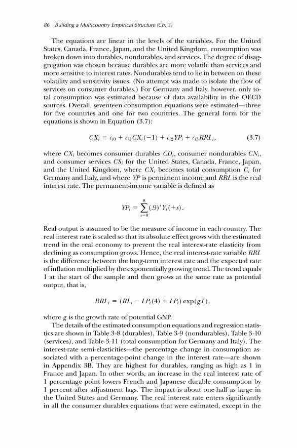
The equations are linear in the levels of the variables. For the UnitedStates, Canada, France, Japan, and the United Kingdom, consumption wasbroken down into durables, nondurables, and services. The degree of disag-gregation was chosen because durables are more volatile than services andmore sensitive to interest rates. Nondurables tend to lie in between on thesevolatility and sensitivity issues. (No attempt was made to isolate the flow ofservices on consumer durables.) For Germany and Italy, however, only to-tal consumption was estimated because of data availability in the OECDsources. Overall, seventeen consumption equations were estimated—threefor five countries and one for two countries. The general form for theequations is shown in Equation (3.7):

CXi 5 ci0 1 ci1CXi(21) 1 ci2YPi 1 ci3RRLi , (3.7)

where CXi becomes consumer durables CDi , consumer nondurables CNi ,and consumer services CSi for the United States, Canada, France, Japan,and the United Kingdom, where CXi becomes total consumption Ci forGermany and Italy, and where YP is permanent income and RRL is the realinterest rate. The permanent-income variable is defined as

YPi 58∑

s50

(.9)sYi(1s).

Real output is assumed to be the measure of income in each country. Thereal interest rate is scaled so that its absolute effect grows with the estimatedtrend in the real economy to prevent the real interest-rate elasticity fromdeclining as consumption grows. Hence, the real interest-rate variable RRLis the difference between the long-term interest rate and the expected rateof inflation multiplied by the exponentially growing trend. The trend equals1 at the start of the sample and then grows at the same rate as potentialoutput, that is,

RRLi 5 (RLi 2 LPi(4) 1 LPi) exp(gT),

where g is the growth rate of potential GNP.The details of the estimated consumption equations and regression statis-

tics are shown in Table 3-8 (durables), Table 3-9 (nondurables), Table 3-10(services), and Table 3-11 (total consumption for Germany and Italy). Theinterest-rate semi-elasticities—the percentage change in consumption as-sociated with a percentage-point change in the interest rate—are shownin Appendix 3B. They are highest for durables, ranging as high as 1 inFrance and Japan. In other words, an increase in the real interest rate of1 percentage point lowers French and Japanese durable consumption by1 percent after adjustment lags. The impact is about one-half as large inthe United States and Germany. The real interest rate enters significantlyin all the consumer durables equations that were estimated, except in the

3.7 Consumption Demand 87

TABLE 3-8 Durables Consumption

The dependent variable is CD. The estimation method is the GMM, and the instru-ments are CD(21), Y(21), Y(22), RL(21), LP(21), LP(22), T , G.

Country Constant CD(21) YP RRL SE R2 DW Sample

U.S. 245.4 0.698 0.040 229.3 8.37 0.95 1.8 71.3(23.7) (0.072) (0.013) (41.2) 84.4

Canada 25.79 0.632 0.047 27.53 0.79 0.97 2.1 71.3(1.56) (0.054) (0.008) (2.74) 84.3

France 241.6 0.344 0.079 234.5 1.51 0.98 1.4 71.3(5.9) (0.077) (0.010) (9.1) 80.4

Japan 24279 0.356 0.041 24098 284.8 0.98 1.6 71.3(459) (0.065) (0.004) (636) 84.3

U.K. 210.2 0.516 0.073 — 1.04 0.72 2.1 71.3(3.5) (0.118) (0.021) 84.3

United Kingdom and in the total consumption equation estimated for Ger-many and for Italy. The real interest rate also enters negatively in consumernondurables in the United States, Canada, and the United Kingdom butwas not found to be significant in services consumption. Overall the effectof real interest rates on consumption is an important part of its effect onaggregate demand, though the effect differs widely among the countries.

The permanent-income variable is very significant in all the equations.Recall that this variable includes current income and expectations of futureincome based on information available in the current period. Hence, the

TABLE 3-9 Nondurables Consumption in Five Countries

The dependent variable is CN. The estimation method is the GMM, and the instru-ments are CN(21), Y(21), Y(22), RL(21), LP(21), LP(22), T , G.

Country Constant CN(21) YP RRL SE R2 DW Sample

U.S. 63.2 0.508 0.098 224.8 4.66 0.99 1.4 71.3(8.4) (0.055) (0.012) (13.1) 84.4

Canada 3.19 0.899 0.015 23.27 0.67 0.99 2.2 71.3(0.84) (0.037) (0.008) (2.24) 84.3

France 25.09 0.330 0.196 — 2.45 0.99 2.1 71.3(4.66) (0.091) (0.028) 80.4

Japan 5180 0.822 0.026 — 821.5 0.98 2.5 71.3(1,019) (0.043) (0.007) 84.3

U.K. 3.44 0.666 0.090 25.00 0.708 0.95 1.9 71.3(1.57) (0.072) (0.020) (2.00) 84.3


TABLE 3-10 Services Consumption in Five Countries

The dependent variable is CS. The estimation method is the GMM, and the instru-ments are CS(21), Y(21), Y(22), RL(21), LP(21), LP(22), T , G.

Country Constant CS(21) YP SE R2 DW Sample

U.S. 224.1 0.906 0.038 4.08 0.99 2.7 71.3(4.4) (0.011) (0.005) 84.4

Canada 21.2 0.912 0.026 0.449 0.99 2.2 71.3(1.2) (0.037) (0.012) 84.3

France 231.4 0.810 0.076 1.33 0.99 2.8 71.3(4.9) (0.026) (0.010) 80.4

Japan 21725 0.692 0.093 809.3 0.99 2.4 71.3(524) (0.072) (0.020) 84.3

U.K. 22.8 0.913 0.032 0.433 0.99 1.8 71.3(1.0) (0.027) (0.008) 84.3

significance of this term is not a contradiction of Hall’s (1978) prediction ofthe forward-looking model that income does not Granger-cause consump-tion. Note, however, that with the lagged dependent variable, the short-runimpact of a change in expected permanent income is smaller than thelong-run impact. (See Appendix 3B for the size of the difference.) Thiscould reflect habit persistence or errors in our permanent-income variable.The greater volatility of durables is reflected in the relatively smaller coef-ficient on the lagged durables consumption compared with lagged servicesconsumption.

3.8 Fixed Investment

Investment demand is assumed to depend on the cost of capital, as measuredby the real rate of interest, and on expected future sales. The measure ofexpected future sales is assumed to have the same form as the measureof expected future income in the consumption equations.

TABLE 3-11 Aggregate Consumption in Germany and Italy

The dependent variable is C. The estimation method is the GMM, and the instrumentsare C(21), Y(21), Y(22), RL(21), LP(21), LP(22), T , G.

Country Constant C(21) YP RRL SE R2 DW Sample

Germany 234.8 0.733 0.177 295.0 9.19 0.98 2.5 71.3(14.7) (0.057) (0.039) (41.3) 84.3

Italy 2388 0.877 0.085 21204 260.3 0.99 1.1 71.3(655) (0.037) (0.028) (609) 84.3

3.8 Fixed Investment 89

TABLE 3-12 Nonresidential Equipment Investment in the United States

The dependent variable is INE. The estimation method is the GMM, and the instru-ments are INE(21), INE(22), Y(21), Y(22), RL(21), LP(21), LP(22), G.

Country Constant INE(21) YP RRL SE R2 DW Sample

U.S. 273.6 0.759 0.043 298.7 7.05 0.96 1.1 71.3(15.3) (0.052) (0.007) (23.6) 84.4

In the United States, fixed investment is disaggregated into three com-ponents: nonresidential equipment, nonresidential structures, residentialstructures. Because of data availability in the OECD publications, less dis-aggregation occurs in the other countries. Equipment and structures areadded to get total nonresidential investment in France, Japan, and theUnited Kingdom. All three components of investment are added to get fixedinvestment for Canada, Germany, and Italy. Overall, twelve fixed-investmentequations were estimated. The general form for all the fixed-investmentequations is as follows:

IXi 5 di0 1 di1IXi(21) 1 di2YPi 1 di3RRLi , (3.8)

where IXi is the nonresidential equipment (INE), the nonresidential struc-ture (INS), and the residential structures (IR) in the United States, whereIXi is the nonresidential (IN ) and residential (IR) investment in France,Japan, and the United Kingdom, and where IXi is the total fixed invest-ment (IF ) in Canada, Germany, and Italy. The variables YP and RL are asdefined for consumption. The equations are linear in the levels of invest-ment. Lagged investment enters the equations, representing either the costof adjusting capital or the periods of time to build capital. The details ofthe twelve estimated equations are shown in Tables 3-12 through 3-16. Thereal interest rate has a negative effect on investment in all the countriesand for almost all components of investment. The semi-elasticity is shownin Appendix 3B and ranges as high as 6 for U.S. nonresidential structures.Of the twelve investment equations estimated, only one did not result ina negative coefficient on the real interest rate; for this equation—Frenchtotal nonresidential investment—the real interest was omitted.

TABLE 3-13 Nonresidential Structures Investment in the United States

The dependent variable is INS. The estimation method is the GMM, and the instru-ments are INS(21), INS(22), Y(21), Y(22), RL(21), LP(21), LP(22), G.

Country Constant INS(21) YP RRL SE R2 DW Sample

U.S. 216.2 0.963 0.007 225.0 3.72 0.95 1.2 71.3(6.8) (0.026) (0.002) (12.2) 84.4


TABLE 3-14 Total Nonresidential Investment in Three Countries

The dependent variable is IN. The estimation method is the GMM, and the instrumentsare IN(21), IN(22), Y(21), Y(22), RL(21), LP(21), LP(22), G.

Country Constant IN(21) YP RRL SE R2 DW Sample

France 11.9 0.812 0.020 — 3.10 0.95 1.7 71.3(3.6) (0.045) (0.007) 84.2

Japan 24755 0.899 0.041 213454 538.6 0.99 1.5 71.3(454) (0.046) (0.007) (1,060) 84.3

U.K. 1.5 0.726 0.034 24.0 0.921 0.65 2.1 71.3(4.1) (0.142) (0.012) (3.3) 84.3

TABLE 3-15 Residential Investment in Four Countries

The dependent variable is IR. The estimation method is the GMM, and the instrumentsare IR(21), IR(22), Y(21), Y(22), RL(21), LP(21), LP(22), G.

Country Constant IR(21) YP RRL SE R2 DW Sample

U.S. 2132.0 0.614 0.063 2269.5 9.61 0.87 0.9 74.1(32.5) (0.062) (0.013) (62.8) 84.4

France 9.2 0.858 — 221.5 0.665 0.98 2.2 71.3(1.4) (0.022) (2.5) 85.2

Japan 2835 0.823 — 22578 733.9 0.72 2.1 71.3(590) (0.038) (865) 85.3

U.K. 2.4 0.728 — 21.33 0.429 0.71 2.0 71.3(0.7) (0.075) (1.03) 85.3

TABLE 3-16 Total Fixed Investment in Three Countries

The dependent variable is IF. The estimation method is the GMM, and the instrumentsare IF(21), IF(22), Y(21), Y(22), RL(21), LP(21), LP(22), G.

Country Constant IF(21) YP RRL SE R2 DW Sample

Canada 22.9 0.933 0.026 29.70 1.61 0.98 1.4 71.3(2.5) (0.049) (0.015) (5.53) 84.3

Germany 21.3 0.810 0.049 2213.8 10.4 0.74 2.2 71.3(13.4) (0.038) (0.016) (80.4) 84.3

Italy 21128 0.907 0.030 23016 299.8 0.89 1.1 71.3(820) (0.029) (0.012) (848) 84.3

3.10 Exports and Imports 91

The expected future sales term is significant in most of the equations,having the highest overall impact in the United States and the lowest inFrance. Over the sample period, there was little trend in the level of res-idential investment in these countries. Note that residential investment inFrance, Japan, and the United Kingdom showed no systematic relationshipto the expected sales variable, and therefore, this term is omitted from theequations.

3.9 Inventory Investment

Inventory investment is assumed to have a different, less forward-looking,functional form than fixed investment. Current sales are assumed to affectthe desired level of inventories. Hence, the change in inventories dependson the change in sales—the usual accelerator model. In addition, we con-sidered the effect of real interest rates on inventory investment. The generalequation for inventory investment is

IIi 5 ei0 1 ei1IIi(21) 1 ei2Yi 1 ei3Yi(21) 1 ei4RRLi , (3.9)

where II is inventory investment, Y is real output, and RRL is again thereal interest rate. The lagged dependent variable was included to reflectany adjustment cost. If ei2 . 0 and ei2 5 2ei3, then only the change in realoutput affects inventory investment.

The estimates are shown in Table 3-17. The real-output terms alwaysenter with opposite signs, suggesting an accelerator model in all countriesexcept Japan. In Japan, the signs are reversed, indicating a buffer stock roleof inventories: when sales decline, inventories rise so that production doesnot fall so much. The real interest rate enters negatively in all the equations.

3.10 Exports and Imports

In each country, exports and imports are measured in real terms in thelocal currency and correspond to the export and import measures usedto compute GNP or GDP by the expenditure approach in the nationalincome accounts. Hence, these flows include not only merchandise tradebut also services. For countries for which output is measured by GNP, theservice component of exports and imports includes factor payments onnongovernment capital and labor because net factor payments from abroadare part of GNP. For countries for which GDP is the output measure, exportsand imports do not include any factor services. Bilateral trade flows betweenthe individual countries in the model were not modeled. In fact, a largepart of exports and imports for each of the seven countries involves tradeflows with developing countries and other countries not included in theG-7. Recall that the model is not a closed-world model in the sense thatall countries or regions in the world are accounted for. Rather, it is anopen-economy model of the seven countries as a group.


TABLE 3-17 Inventory Investment

The dependent variable is II. The estimation method is the GMM for all countriesexcept Japan, for which 2SLS was used. The instruments are II(21), II(22), Y(21),Y(22), RL(21), LP(21), LP(22), G.

Country Constant II(21) Y Y(21) RRL SE R2 DW

U.S. 215.4 0.656 0.207 20.201 286.3 17.3 0.59 2.1(23.6) (0.047) (0.083) (0.084) (59.2)

Canada 28.4 0.715 0.632 20.605 224.3 2.7 0.67 2.2(3.3) (0.043) (0.107) (0.104) (7.6)

France 20.7 0.699 0.156 20.151 245.0 6.8 0.53 1.8(13.2) (0.099) (0.195) (0.187) (21.5)

Germany 7.7 0.326 0.178 20.171 2261 13.5 0.30 1.9(19.0) (0.138) (0.181) (0.193) (156)

Italy 23462 0.543 0.561 20.515 27551 752.0 0.65 1.9(1,089) (0.147) (0.191) (0.200) (2309)

Japan 21064 0.296 20.306 0.323 216349 1270 0.31 1.6(1,559) (0.129) (0.139) (0.141) (4994)

U.K. 0.65 0.639 0.034 20.036 22.52 2.06 0.45 1.9(2.6) (0.123) (0.144) (0.144) (7.6)

Note: Sample periods were 71.3 to 85.3 for all countries except the United States (85.4) andFrance (85.2).

The export and import-demand equations have the following log-linearform:

LEXi 5 fi0 1 fi1LEXi(21) 1 fi2(LPEXi 2 LPIMi) 1 fi3LYWi (3.10)

LIMi 5 gi0 1 gi1LIMi(21) 1 gi2(LPIMi 2 LPi) 1 gi3LYi , (3.11)

where LEX is the log of exports, LPEX , LPIM , and LP are the price defla-tors for exports, imports, and output respectively, and LYW is the log of aweighted average of output in the other countries.

The relative price variable for exports is the ratio of export prices PEXto import prices PIM . The ratio of the import price to the domestic pricedeflator is used in the import equation. Alternative relative price ratios(such as LPEX -LP for exports and LPIM -LPEX for imports) were tried inthe preliminary statistical work. These measures were chosen simply becausethey gave more plausible and better-fitting equations on average in all thecountries.10

10The log ratio LFP -LP was also used for both exports and imports but performed poorlycompared to measures that explicitly included export or import prices. The fact that LFP -LPdid not work well necessitated the estimation of equations LPEX and LPIM as already discussedin Section 3.4.

3.11 Money Demand 93

TABLE 3-18 Export Demand

The dependent variable is LEX, and the estimation method is OLSQ (ordinary leastsquares).

Country Constant LEX(21) LPEX-LPIM LYW SE R2 DW Sample

U.S. 20.70 0.794 20.151 0.230 0.034 0.98 1.7 71.2(0.63) (0.094) (0.129) (0.125) 86.2

Canada 26.63 0.581 20.325 1.015 0.033 0.98 2.0 71.2(1.34) (0.088) (0.104) (0.205) 86.2

France 25.69 0.509 20.376 0.999 0.016 0.99 1.9 71.2(0.91) (0.071) (0.071) (0.154) 86.2

Germany 22.94 0.532 20.340 0.684 0.024 0.99 2.0 71.2(0.66) (0.080) (0.103) (0.129) 86.2

Italy 21.79 0.704 20.080 0.595 0.032 0.98 1.8 71.2(0.68) (0.084) (0.070) (0.184) 86.2

Japan 20.82 0.814 20.153 0.372 0.029 0.99 1.5 71.2(0.72) (0.043) (0.039) (0.139) 86.2

U.K. 26.12 0.131 20.370 1.129 0.031 0.96 2.1 71.2(0.86) (0.112) (0.076) (0.151) 86.2

The demand variable in the import equations is measured by real output.The demand variable in the export equations is a trade-weighted averageof real output in the other six countries. In all the equations, the role ofthe lagged dependent variable is to approximate the slow adjustment ofimporters and consumers to changes in relative prices.

The details of the estimated equations are listed in Tables 3-18 and 3-19.The equations are all estimated with ordinary least squares. Surprisingly,there appeared to be little relationship between relative prices and importdemand in Germany and, hence, this term was omitted from the Germanimport equation. With this exception, the sign of the price variable is neg-ative for all of the export- and import-demand equations. The elasticities(shown in Appendix 3B) vary considerably across the countries. Long-runincome elasticities are all greater than 1, reflecting the growing importanceof trade during the last twenty years. The significant lagged dependent vari-able shows, however, that adjustments to either price or income changesoccur with a lag.

3.11 Money Demand

Finally we consider the money-demand equation, which is assumed to havethe traditional Cagan semi-log form for all countries just like in Chapter 1.The log of real-money demand is assumed to depend on the log of real


TABLE 3-19 Import Demand

The dependent variable is LIM, and the estimation method is OLSQ (ordinary leastsquares).

Country Constant LIM(21) LPIM-LP LY SE R2 DW Sample

U.S. 27.00 0.440 20.216 1.275 0.032 0.98 1.7 71.2(0.97) (0.080) (0.036) (0.177) 86.4

Canada 21.48 0.679 20.100 0.498 0.032 0.98 1.4 71.2(0.46) (0.076) (0.075) (0.134) 86.3

France 23.16 0.688 20.148 0.698 0.024 0.99 1.6 71.2(0.94) (0.079) (0.044) (0.196) 86.2

Germany 25.39 0.291 1.325 0.024 0.98 2.2 71.2(0.81) (0.100) (0.191) 86.3

Italy 27.57 0.414 20.190 1.177 0.034 0.98 1.5 71.2(1.24) (0.093) (0.039) (0.187) 86.3

Japan 20.35 0.902 20.081 0.111 0.032 0.97 1.7 71.2(0.32) (0.059) (0.026) (0.051) 86.3

U.K. 22.14 0.651 20.061 0.657 0.036 0.94 2.0 71.2(0.70) (0.097) (0.041) (0.194) 86.3

income, the level of the short-term interest rate, and on the log of laggedreal-money balances. Using a common functional form for all countriespermits easy comparison across countries and seems to work well as anapproximation, although of course there have been large shifts in moneydemand because of technological and regulatory changes. The equationfor money demand is given by

L(Mi/Pi) 5 ai0 1 ai1L(Mi(21)/Pi(21)) 1 ai2RSi 1 ai3LYi , (3.12)

where M is money supply (M1), and where all other variables have beendefined previously. Real output is the measure of income or scale variable.Lagged real-money balances appear in the equation to account for slowadjustment. There are no lead variables in these equations. A time trendstarting in 1982:1 was added to the U.S. and U.K. equations to capture theeffects of regulatory change and financial innovation in the 1980s.

The estimates are shown in Table 3-20. The equations were estimatedby two-stage least squares. The only significant sign of serial correlation inthese equations is in Italy (but recall that there is a time-trend variable forthe United States and United Kingdom). The signs on the interest ratesand income variable are all correct and usually statistically significant. Thelarge coefficient on the lagged dependent variable indicates that the short-run elasticities are much smaller than the long-run elasticities (shown inAppendix 3B).

3.12 Identities and Potential GNP 95

TABLE 3-20 Money Demand

The dependent variable is LMP. The estimation method is two-stage least squares,and the instruments are LM(21), LM(22), LP(21), LP(22), LY(21), LY(22), RS(21),G. A linear time trend starting in 1982:1 is included in the equations for the UnitedStates and the United Kingdom.

Country Constant LMP(21) RS LY SE R2 DW Sample

U.S. 20.009 0.953 20.224 0.040 0.009 0.98 1.6 71.3(0.413) (0.036) (0.055) (0.031) 86.4

Canada 0.060 0.937 20.511 0.033 0.019 0.93 2.1 71.3(0.225) (0.039) (0.106) (0.026) 86.3

France 0.671 0.683 20.316 0.167 0.010 0.87 1.7 78.3(0.544) (0.116) (0.097) (0.080) 86.2

Germany 21.241 0.697 20.646 0.403 0.020 0.98 2.5 71.3(0.497) (0.090) (0.120) (0.133) 86.3

Italy 0.289 0.895 20.387 0.077 0.016 0.93 1.2 71.3(0.386) (0.037) (0.068) (0.030) 86.3

Japan 1.107 0.750 20.479 0.139 0.016 0.99 1.8 71.3(0.194) (0.059) (0.090) (0.043) 86.3

U.K. 20.778 0.916 20.778 0.212 0.020 0.97 1.9 71.3(0.662) (0.034) (0.173) (0.116) 86.2

3.12 Identities and Potential GNP

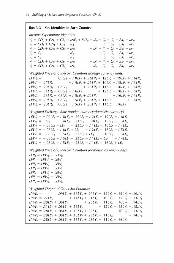
The remaining equations of the model include several identities and the def-inition of aggregate supply. The income-expenditure identities are shownbelow in Equation (3.13), which is a useful summary of the degree of disag-gregation of aggregate demand used in each country:

Y0 5 CD0 1 CN0 1 CS0 1 INE0 1 INS0 1 IR0 1 II0 1 G0 1 EX0 2 IM0

Y1 5 CD1 1 CN1 1 CS1 1 IF1 1 II1 1 G1 1 EX1 2 IM1

Y2 5 CD2 1 CN2 1 CS2 1 IN2 1 IR2 1 II2 1 G2 1 EX2 2 IM2

Y3 5 C3 1 IF3 1 II3 1 G3 1 EX3 2 IM3

Y4 5 C4 1 IF4 1 II4 1 G4 1 EX4 2 IM4


Y6 5 CD6 1 CN6 1 CS6 1 IN6 1 IR6 1 II6 1 G6 1 EX6 2 IM6.

(3.13)

Many of the equations in the model are estimated in log form, with the mainexceptions being consumption and investment. These income-expenditureidentities obviously need to be written in linear form. The mixture of linear


Box 3-3 Key Identities in Each Country

Income-Expenditure IdentitiesY0 5 CD0 1 CN0 1 CS0 1 INE0 1 INS0 1 IR0 1 II0 1 G0 1 EX0 2 IM0

Y1 5 CD1 1 CN1 1 CS1 1 IF1 1 II1 1 G1 1 EX1 2 IM1


Y3 5 C3 1 IF3 1 II3 1 G3 1 EX3 2 IM3

Y4 5 C4 1 IF4 1 II4 1 G4 1 EX4 2 IM4



Weighted Price of Other Six Countries (foreign currency units)LPW0 5 .09LP1 1 .18LP2 1 .26LP3 1 .12LP4 1 .19LP5 1 .16LP6

LPW1 5 .27LP0 1 .14LP2 1 .21LP3 1 .10LP4 1 .15LP5 1 .13LP6






Weighted Exchange Rate (foreign currency/domestic currency)LEW0 5 2.09LE1 2 .18LE2 2 .26LE3 2 .12LE4 2 .19LE5 2 .16LE6

LEW1 5 LE1 2 .14LE2 2 .21LE3 2 .10LE4 2 .15LE5 2 .13LE6

LEW2 5 2.08LE1 1 LE2 2 .23LE3 2 .11LE4 2 .16LE5 2 .14LE6

LEW3 5 2.08LE1 2 .16LE2 1 LE3 2 .12LE4 2 .18LE5 2 .15LE6

LEW4 5 2.08LE1 2 .15LE2 2 .22LE3 1 LE4 2 .16LE5 2 .13LE6

LEW5 5 2.08LE1 2 .15LE2 2 .23LE3 2 .11LE4 1 LE5 2 .14LE6

LEW6 5 2.08LE1 2 .15LE2 2 .23LE3 2 .11LE4 2 .16LE5 1 LE6

Weighted Price of Other Six Countries (domestic currency units)LFP0 5 LPW0 2 LEW0

LFP1 5 LPW1 2 LEW1

LFP2 5 LPW2 2 LEW2

LFP3 5 LPW3 2 LEW3

LFP4 5 LPW4 2 LEW4

LFP5 5 LPW5 2 LEW5

LFP6 5 LPW6 2 LEW6

Weighted Output of Other Six CountriesLYW0 5 .09LY1 1 .18LY2 1 .26LY3 1 .12LY4 1 .19LY5 1 .16LY6

LYW1 5 .27LY0 1 .14LY2 1 .21LY3 1 .10LY4 1 .15LY5 1 .13LY6






3.13 The Whole Model 97

equations and nonlinear equations means that the entire model cannot bereduced to either a log-linear or a linear form.

The remaining identities in the model simply define several weightedaverages of other variables. These are shown in Box 3-3. They include theweighted price LPWi , the weighted foreign price LFPi , and the weightedoutput LYWi in each country. Each of these variables has already beendiscussed.

Finally, potential output is assumed to be growing exponentially. For thepurposes of simulation and structural residual calculation during the sampleperiod, the exponential trend is assumed to be constant and was estimatedby regressing the log of real output on a linear trend. The estimated growthrates in percent per year were 2.4 for the United States, 3.2 for Canada,2.5 for France, 2.0 for Germany, 2.2 for Italy, 4.2 for Japan, and 1.5 for theUnited Kingdom. No explicit attempt was made in the simulations to changethe potential growth rate either exogenously or as a function of policy. Thefocus of this model is on economic fluctuations around this potential level.Of course, this does not mean that potential output or its growth rateare unaffected by macropolicy. The volatility of inflation surely affects realoutput, for example. But in order to focus on fluctuations, I abstract fromthese effects. In my judgment, this abstraction does not detract from theanalysis.

3.13 The Whole Model

Equations (3.1) through (3.13), along with the definitions of the weightedaverages of prices, exchange rates, and output, define the entire multicoun-try model. There are a total of ninety-eight estimated stochastic equations:twenty-eight describing wage and price behavior, fifty describing aggregatedemand, and twenty describing financial markets. These are summarized inBox 3-2. The estimation of most of these equations required econometricmethods to deal with rational expectations that did not exist ten years ago.In addition, there are thirty identities, summarized in Box 3-3, and sevenequations defining the long-run growth trend of GNP or GDP.

Although I have not emphasized it, there are a number of remarkablecharacteristics about these equations. For example, the real interest rateappears to be statistically and quantitatively significant in a large number ofequations, including those relating to inventories and durables consump-tion. The signs of the price variables in the exports, imports, and money-demand equations are correct in virtually every country. Perhaps most re-markable is the fact that essentially the same functional form worked wellfor all countries.

Although I have presented the estimated stochastic equations, I have notyet described the stochastic disturbances to these equations, which are es-sential for policy analysis. This requires considering the model as a whole. Inthe next chapter I discuss how the entire model is put together, solved, and


simulated, along with the estimation of the stochastic disturbance structure.In doing so I will rely on the nonlinear extended path method for solvingand simulating rational expectation models as described in Chapter 1.

Reference Notes

The chapter makes no attempt to compare the structure of this model withother econometric models, either rational or conventional. Several suchcomparisons are available in the literature, however. An early version of themulticountry model was presented at the first Brookings Model ComparisonProject conference in 1986 and published in Bryant, et al. (1988a). Alongwith many other things, that useful volume provides a brief comparisonof this model with other multicountry models in existence as of that time.Several useful analytic comparisons of this model with conventional modelsare found in Helliwell, Cockerline, and Lafrance (1990) and Brayton andMarquez (1990), who focus on the financial sector, and in Visco (1991),who focuses on the wage-price sector.

The properties of most of the instrumental variable-estimation tech-niques used in this chapter are found in any advanced econometricstextbook. The generalized method of moments estimator designed toestimate rational expectations models in time-series applications is derivedby Hansen (1982).

Many papers have been written on the estimation of single equationsfor the components of consumption and investment, inventories, and netexports, examining issues such as real-interest-rate sensitivity, lag structure,and income elasticities. No attempt has been made to compare systemati-cally my equations with these others. Most of the other studies have focusedon a single country and have used different data and different functionalforms.

ii an international macroeconomic frameworkjohntayl/macpolbk/chap3.pdf · · 2001-01-183 building...

Documents