1

IES <Virtual Environment>

Tutorial

Vista (Version 6.0)

Introduction This tutorial will show you how to use Vista to review the results from a dynamic thermal simulation performed using ApacheSim. For more detailed help you can use the Help menu within the specific IES application, and also you can refer to the product manuals installed with the IES software.

2

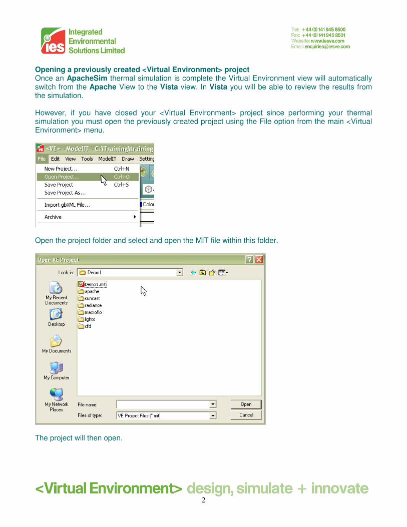
Opening a previously created <Virtual Environment> project Once an ApacheSim thermal simulation is complete the Virtual Environment view will automatically switch from the Apache View to the Vista view. In Vista you will be able to review the results from the simulation. However, if you have closed your <Virtual Environment> project since performing your thermal simulation you must open the previously created project using the File option from the main <Virtual Environment> menu.

Open the project folder and select and open the MIT file within this folder.

The project will then open.

3

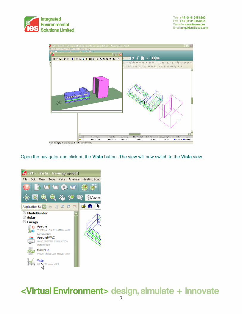
Open the navigator and click on the Vista button. The view will now switch to the Vista view.

4

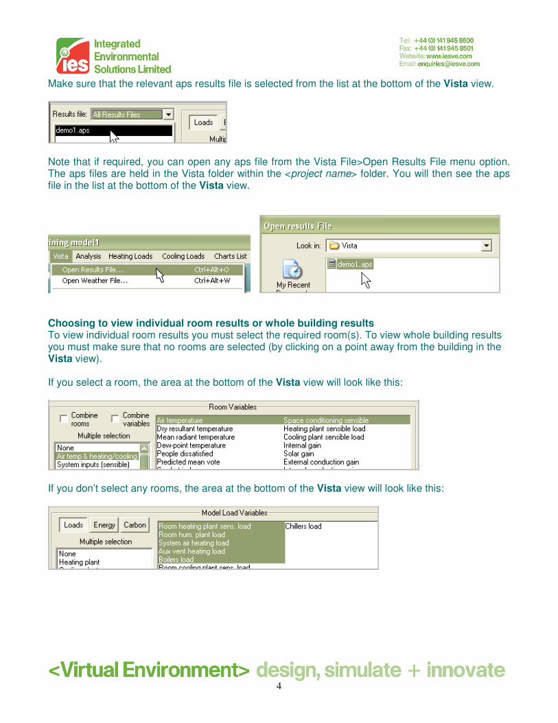
Make sure that the relevant aps results file is selected from the list at the bottom of the Vista view.

Note that if required, you can open any aps file from the Vista File>Open Results File menu option. The aps files are held in the Vista folder within the <project name> folder. You will then see the aps file in the list at the bottom of the Vista view.

Choosing to view individual room results or whole building results To view individual room results you must select the required room(s). To view whole building results you must make sure that no rooms are selected (by clicking on a point away from the building in the Vista view). If you select a room, the area at the bottom of the Vista view will look like this:

If you don’t select any rooms, the area at the bottom of the Vista view will look like this:

5

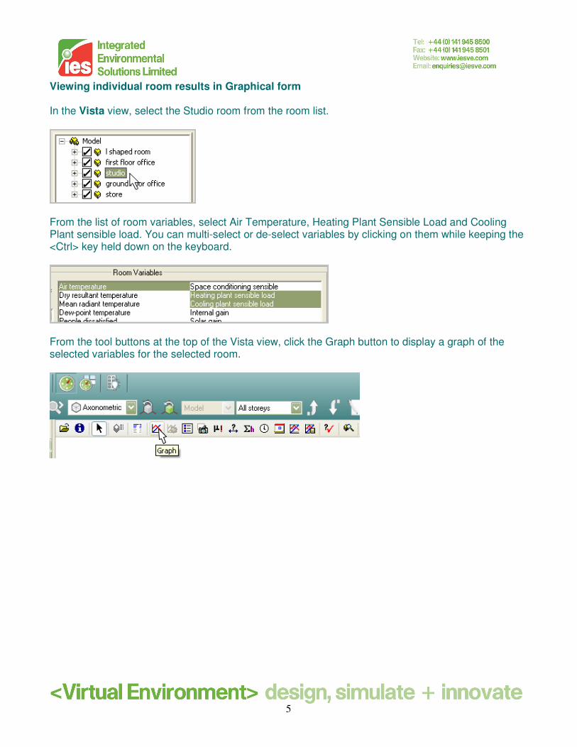
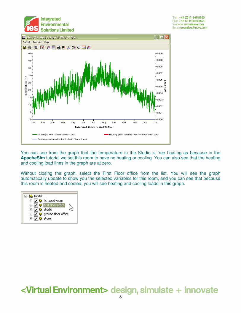
Viewing individual room results in Graphical form In the Vista view, select the Studio room from the room list.

From the list of room variables, select Air Temperature, Heating Plant Sensible Load and Cooling Plant sensible load. You can multi-select or de-select variables by clicking on them while keeping the <Ctrl> key held down on the keyboard.

From the tool buttons at the top of the Vista view, click the Graph button to display a graph of the selected variables for the selected room.

6

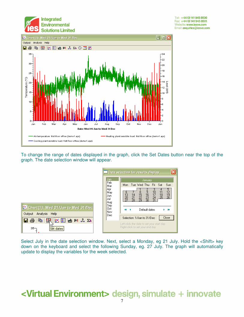
You can see from the graph that the temperature in the Studio is free floating as because in the ApacheSim tutorial we set this room to have no heating or cooling. You can also see that the heating and cooling load lines in the graph are at zero. Without closing the graph, select the First Floor office from the list. You will see the graph automatically update to show you the selected variables for this room, and you can see that because this room is heated and cooled, you will see heating and cooling loads in this graph.

7

To change the range of dates displayed in the graph, click the Set Dates button near the top of the graph. The date selection window will appear.

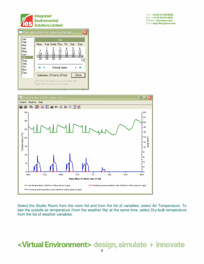
Select July in the date selection window. Next, select a Monday, eg 21 July. Hold the <Shift> key down on the keyboard and select the following Sunday, eg. 27 July. The graph will automatically update to display the variables for the week selected.

8

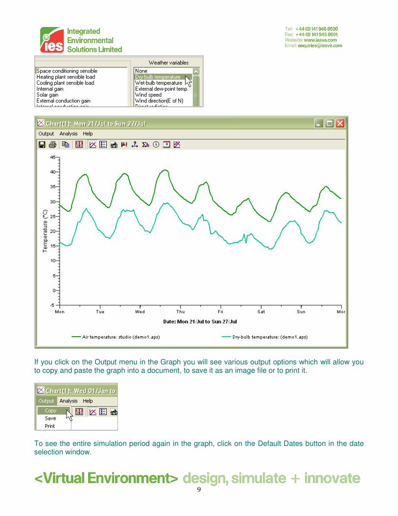
Select the Studio Room from the room list and from the list of variables, select Air Temperature. To see the outside air temperature (from the weather file) at the same time, select Dry-bulb temperature from the list of weather variables.

9

If you click on the Output menu in the Graph you will see various output options which will allow you to copy and paste the graph into a document, to save it as an image file or to print it.

To see the entire simulation period again in the graph, click on the Default Dates button in the date selection window.

10

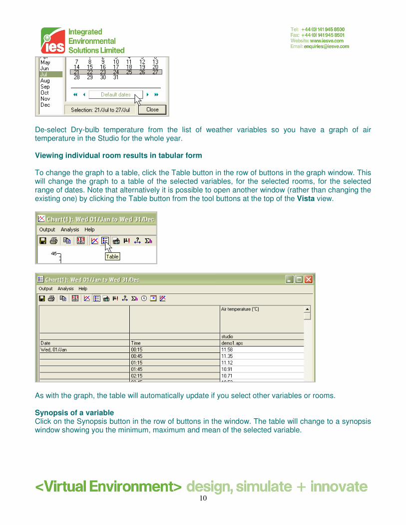
De-select Dry-bulb temperature from the list of weather variables so you have a graph of air temperature in the Studio for the whole year. Viewing individual room results in tabular form To change the graph to a table, click the Table button in the row of buttons in the graph window. This will change the graph to a table of the selected variables, for the selected rooms, for the selected range of dates. Note that alternatively it is possible to open another window (rather than changing the existing one) by clicking the Table button from the tool buttons at the top of the Vista view.

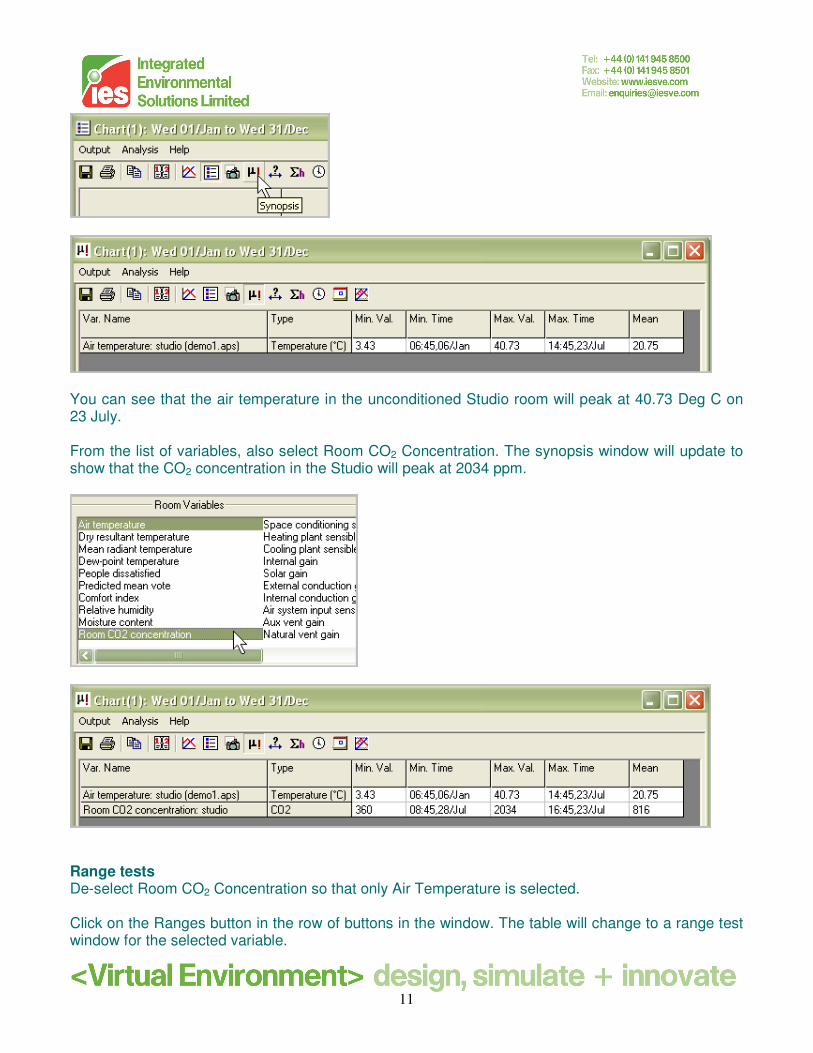
As with the graph, the table will automatically update if you select other variables or rooms. Synopsis of a variable Click on the Synopsis button in the row of buttons in the window. The table will change to a synopsis window showing you the minimum, maximum and mean of the selected variable.

11

You can see that the air temperature in the unconditioned Studio room will peak at 40.73 Deg C on 23 July. From the list of variables, also select Room CO2 Concentration. The synopsis window will update to show that the CO2 concentration in the Studio will peak at 2034 ppm.

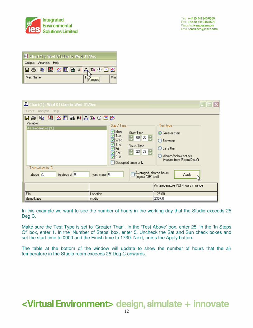
Range tests De-select Room CO2 Concentration so that only Air Temperature is selected. Click on the Ranges button in the row of buttons in the window. The table will change to a range test window for the selected variable.

12

In this example we want to see the number of hours in the working day that the Studio exceeds 25 Deg C. Make sure the Test Type is set to ‘Greater Than’. In the ‘Test Above’ box, enter 25. In the ‘In Steps Of’ box, enter 1. In the ‘Number of Steps’ box, enter 5. Uncheck the Sat and Sun check boxes and set the start time to 0900 and the Finish time to 1730. Next, press the Apply button. The table at the bottom of the window will update to show the number of hours that the air temperature in the Studio room exceeds 25 Deg C onwards.

13

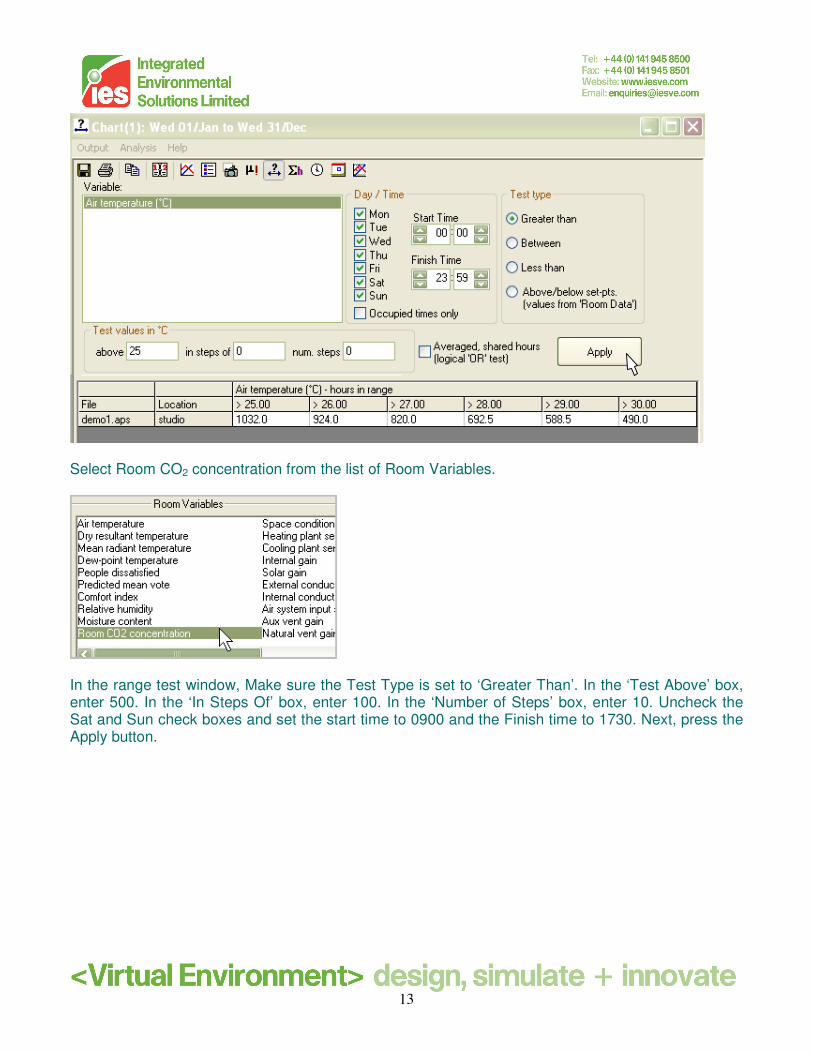
Select Room CO2 concentration from the list of Room Variables.

In the range test window, Make sure the Test Type is set to ‘Greater Than’. In the ‘Test Above’ box, enter 500. In the ‘In Steps Of’ box, enter 100. In the ‘Number of Steps’ box, enter 10. Uncheck the Sat and Sun check boxes and set the start time to 0900 and the Finish time to 1730. Next, press the Apply button.

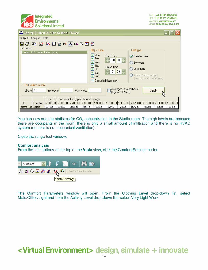
14

You can now see the statistics for CO2 concentration in the Studio room. The high levels are because there are occupants in the room, there is only a small amount of infiltration and there is no HVAC system (so here is no mechanical ventilation). Close the range test window. Comfort analysis From the tool buttons at the top of the Vista view, click the Comfort Settings button

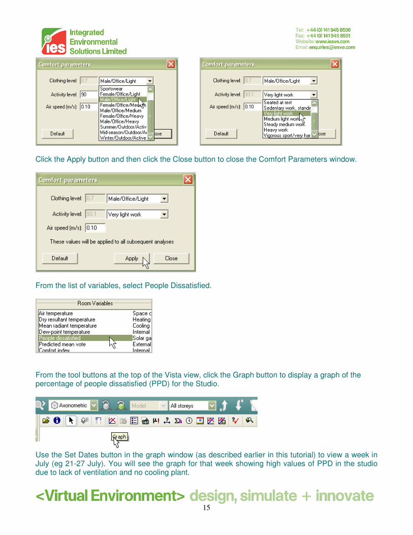
The Comfort Parameters window will open. From the Clothing Level drop-down list, select Male/Office/Light and from the Activity Level drop-down list, select Very Light Work.

15

Click the Apply button and then click the Close button to close the Comfort Parameters window.

From the list of variables, select People Dissatisfied.

From the tool buttons at the top of the Vista view, click the Graph button to display a graph of the percentage of people dissatisfied (PPD) for the Studio.

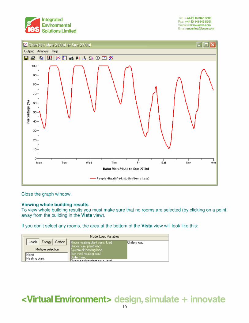
Use the Set Dates button in the graph window (as described earlier in this tutorial) to view a week in July (eg 21-27 July). You will see the graph for that week showing high values of PPD in the studio due to lack of ventilation and no cooling plant.

16

Close the graph window. Viewing whole building results To view whole building results you must make sure that no rooms are selected (by clicking on a point away from the building in the Vista view). If you don’t select any rooms, the area at the bottom of the Vista view will look like this:

17

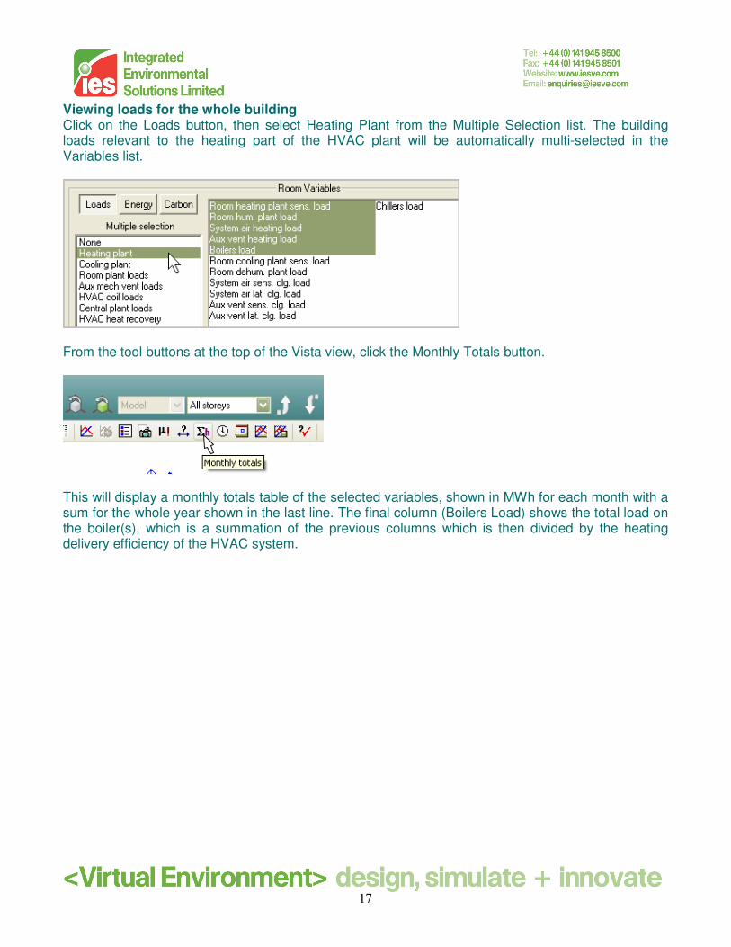
Viewing loads for the whole building Click on the Loads button, then select Heating Plant from the Multiple Selection list. The building loads relevant to the heating part of the HVAC plant will be automatically multi-selected in the Variables list.

From the tool buttons at the top of the Vista view, click the Monthly Totals button.

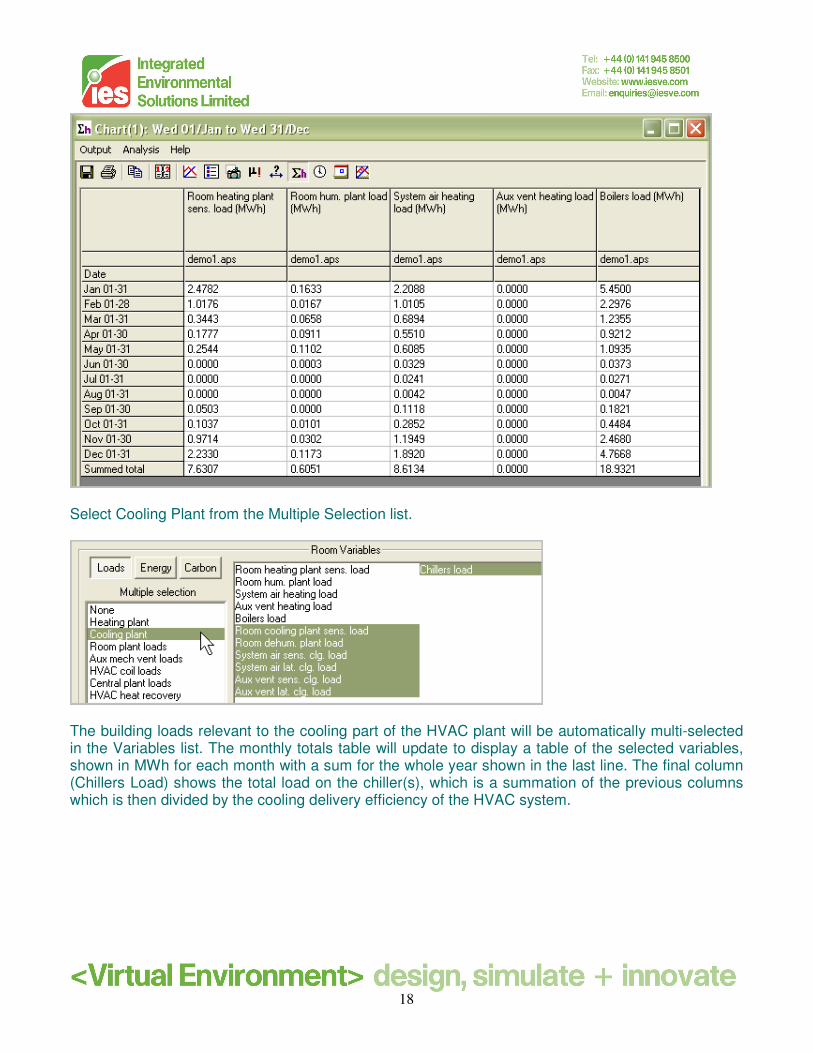
This will display a monthly totals table of the selected variables, shown in MWh for each month with a sum for the whole year shown in the last line. The final column (Boilers Load) shows the total load on the boiler(s), which is a summation of the previous columns which is then divided by the heating delivery efficiency of the HVAC system.

18

Select Cooling Plant from the Multiple Selection list.

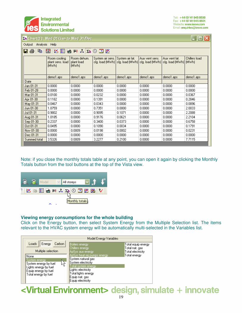
The building loads relevant to the cooling part of the HVAC plant will be automatically multi-selected in the Variables list. The monthly totals table will update to display a table of the selected variables, shown in MWh for each month with a sum for the whole year shown in the last line. The final column (Chillers Load) shows the total load on the chiller(s), which is a summation of the previous columns which is then divided by the cooling delivery efficiency of the HVAC system.

19

Note: if you close the monthly totals table at any point, you can open it again by clicking the Monthly Totals button from the tool buttons at the top of the Vista view.

Viewing energy consumptions for the whole building Click on the Energy button, then select System Energy from the Multiple Selection list. The items relevant to the HVAC system energy will be automatically multi-selected in the Variables list.

20

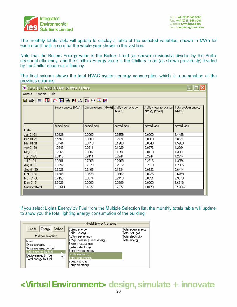
The monthly totals table will update to display a table of the selected variables, shown in MWh for each month with a sum for the whole year shown in the last line. Note that the Boilers Energy value is the Boilers Load (as shown previously) divided by the Boiler seasonal efficiency, and the Chillers Energy value is the Chillers Load (as shown previously) divided by the Chiller seasonal efficiency. The final column shows the total HVAC system energy consumption which is a summation of the previous columns.

If you select Lights Energy by Fuel from the Multiple Selection list, the monthly totals table will update to show you the total lighting energy consumption of the building.

21

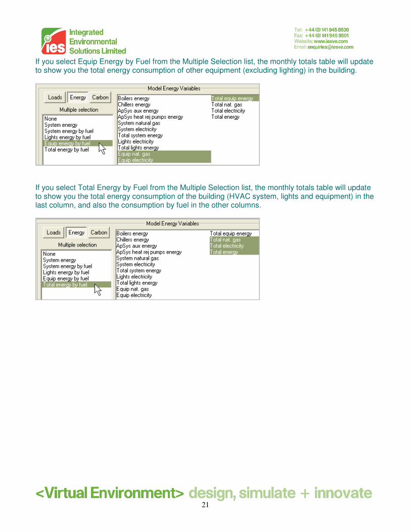
If you select Equip Energy by Fuel from the Multiple Selection list, the monthly totals table will update to show you the total energy consumption of other equipment (excluding lighting) in the building.

If you select Total Energy by Fuel from the Multiple Selection list, the monthly totals table will update to show you the total energy consumption of the building (HVAC system, lights and equipment) in the last column, and also the consumption by fuel in the other columns.

22

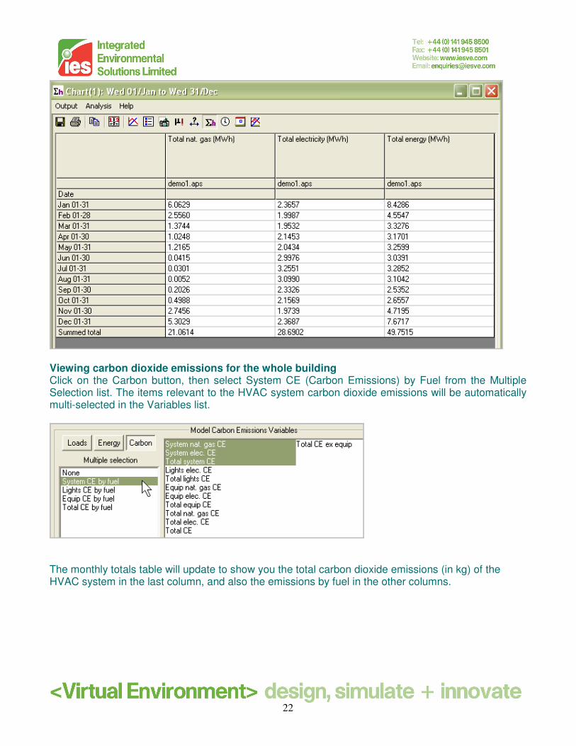
Viewing carbon dioxide emissions for the whole building Click on the Carbon button, then select System CE (Carbon Emissions) by Fuel from the Multiple Selection list. The items relevant to the HVAC system carbon dioxide emissions will be automatically multi-selected in the Variables list.

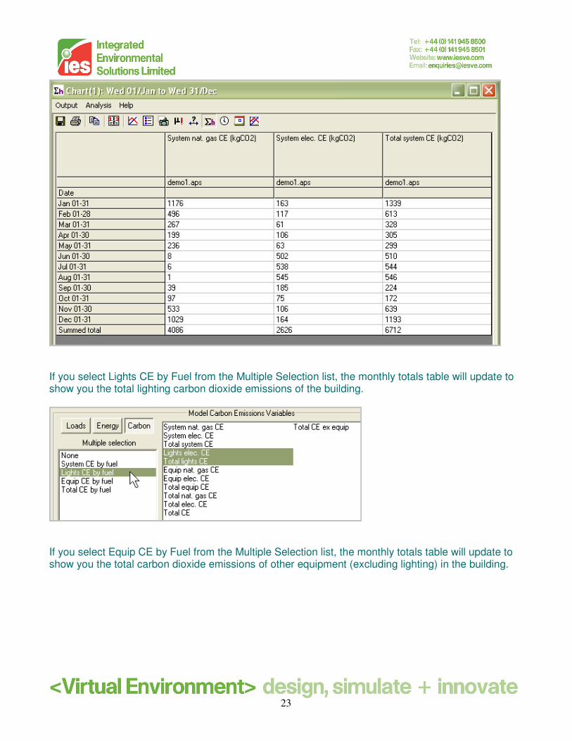
The monthly totals table will update to show you the total carbon dioxide emissions (in kg) of the HVAC system in the last column, and also the emissions by fuel in the other columns.

23

If you select Lights CE by Fuel from the Multiple Selection list, the monthly totals table will update to show you the total lighting carbon dioxide emissions of the building.

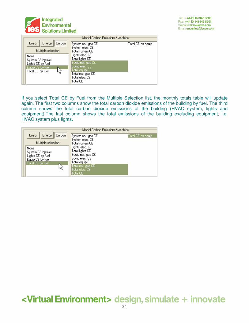
If you select Equip CE by Fuel from the Multiple Selection list, the monthly totals table will update to show you the total carbon dioxide emissions of other equipment (excluding lighting) in the building.

24

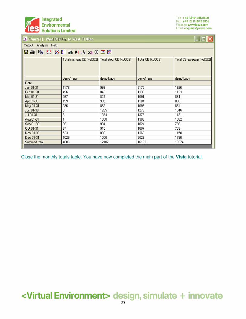
If you select Total CE by Fuel from the Multiple Selection list, the monthly totals table will update again. The first two columns show the total carbon dioxide emissions of the building by fuel. The third column shows the total carbon dioxide emissions of the building (HVAC system, lights and equipment).The last column shows the total emissions of the building excluding equipment, i.e. HVAC system plus lights.

25

Close the monthly totals table. You have now completed the main part of the Vista tutorial.

26

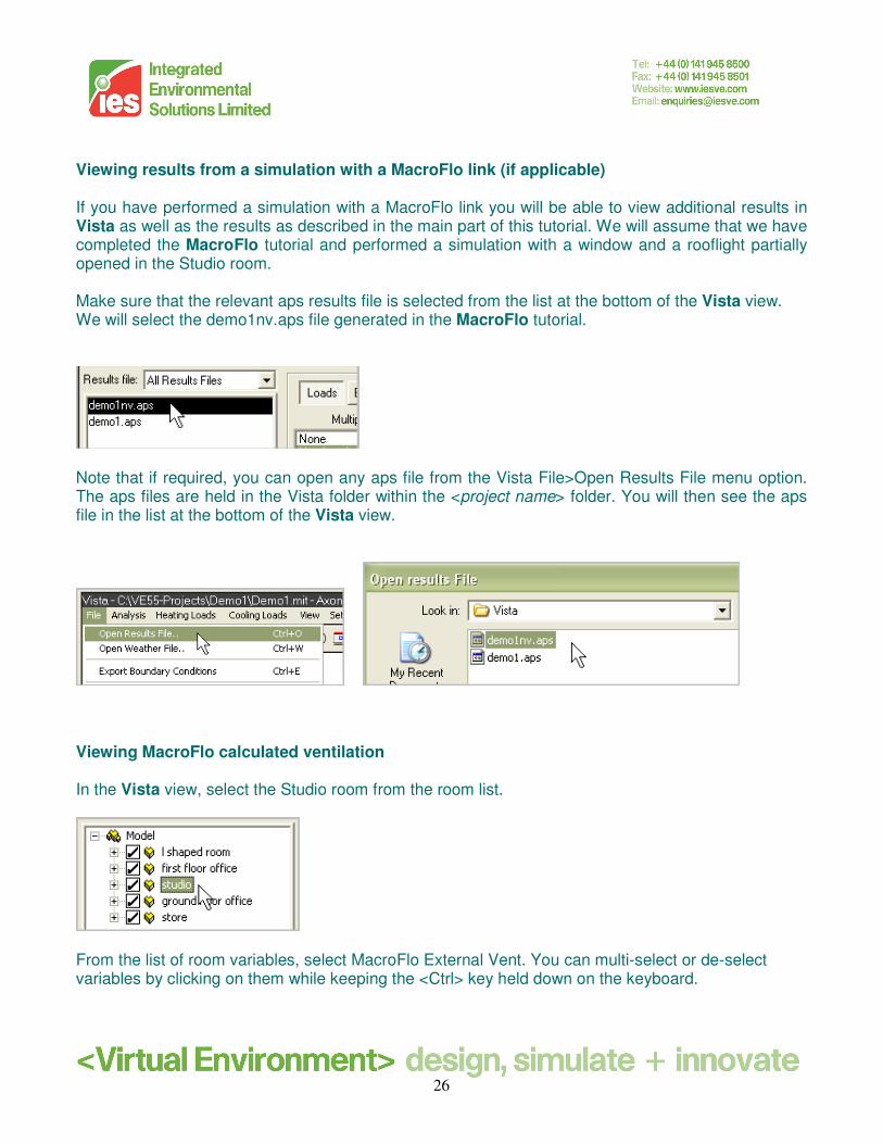
Viewing results from a simulation with a MacroFlo link (if applicable) If you have performed a simulation with a MacroFlo link you will be able to view additional results in Vista as well as the results as described in the main part of this tutorial. We will assume that we have completed the MacroFlo tutorial and performed a simulation with a window and a rooflight partially opened in the Studio room. Make sure that the relevant aps results file is selected from the list at the bottom of the Vista view. We will select the demo1nv.aps file generated in the MacroFlo tutorial.

Note that if required, you can open any aps file from the Vista File>Open Results File menu option. The aps files are held in the Vista folder within the <project name> folder. You will then see the aps file in the list at the bottom of the Vista view.

Viewing MacroFlo calculated ventilation In the Vista view, select the Studio room from the room list.

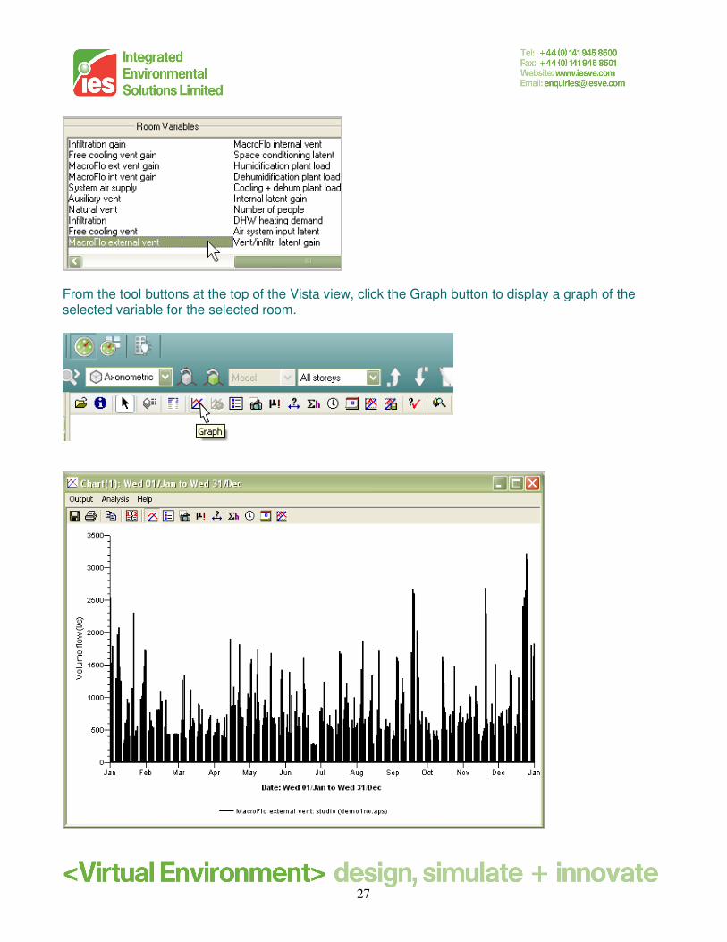
From the list of room variables, select MacroFlo External Vent. You can multi-select or de-select variables by clicking on them while keeping the <Ctrl> key held down on the keyboard.

27

From the tool buttons at the top of the Vista view, click the Graph button to display a graph of the selected variable for the selected room.

28

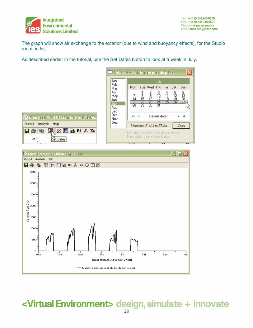
The graph will show air exchange to the exterior (due to wind and buoyancy effects), for the Studio room, in l/s. As described earlier in the tutorial, use the Set Dates button to look at a week in July.

29

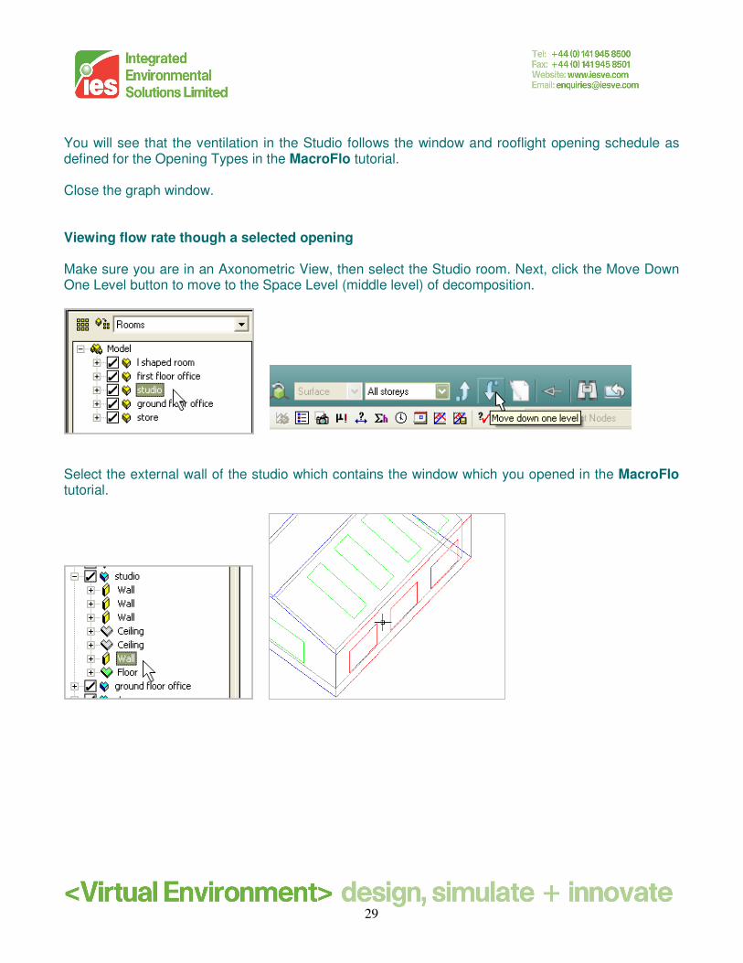
You will see that the ventilation in the Studio follows the window and rooflight opening schedule as defined for the Opening Types in the MacroFlo tutorial. Close the graph window. Viewing flow rate though a selected opening Make sure you are in an Axonometric View, then select the Studio room. Next, click the Move Down One Level button to move to the Space Level (middle level) of decomposition.

Select the external wall of the studio which contains the window which you opened in the MacroFlo tutorial.

30

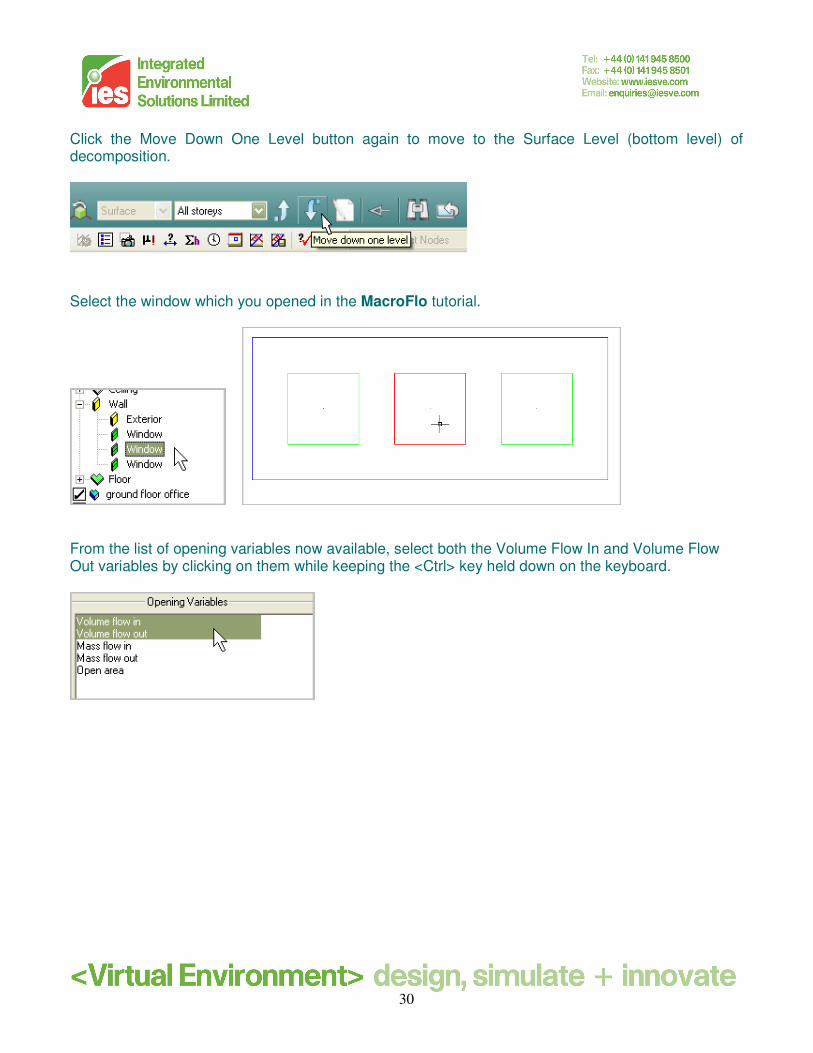
Click the Move Down One Level button again to move to the Surface Level (bottom level) of decomposition.

Select the window which you opened in the MacroFlo tutorial.

From the list of opening variables now available, select both the Volume Flow In and Volume Flow Out variables by clicking on them while keeping the <Ctrl> key held down on the keyboard.

31

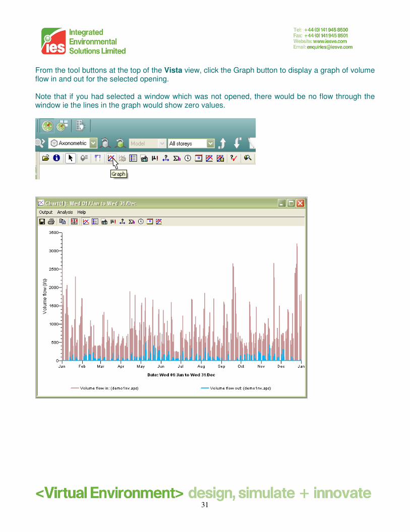
From the tool buttons at the top of the Vista view, click the Graph button to display a graph of volume flow in and out for the selected opening. Note that if you had selected a window which was not opened, there would be no flow through the window ie the lines in the graph would show zero values.

32

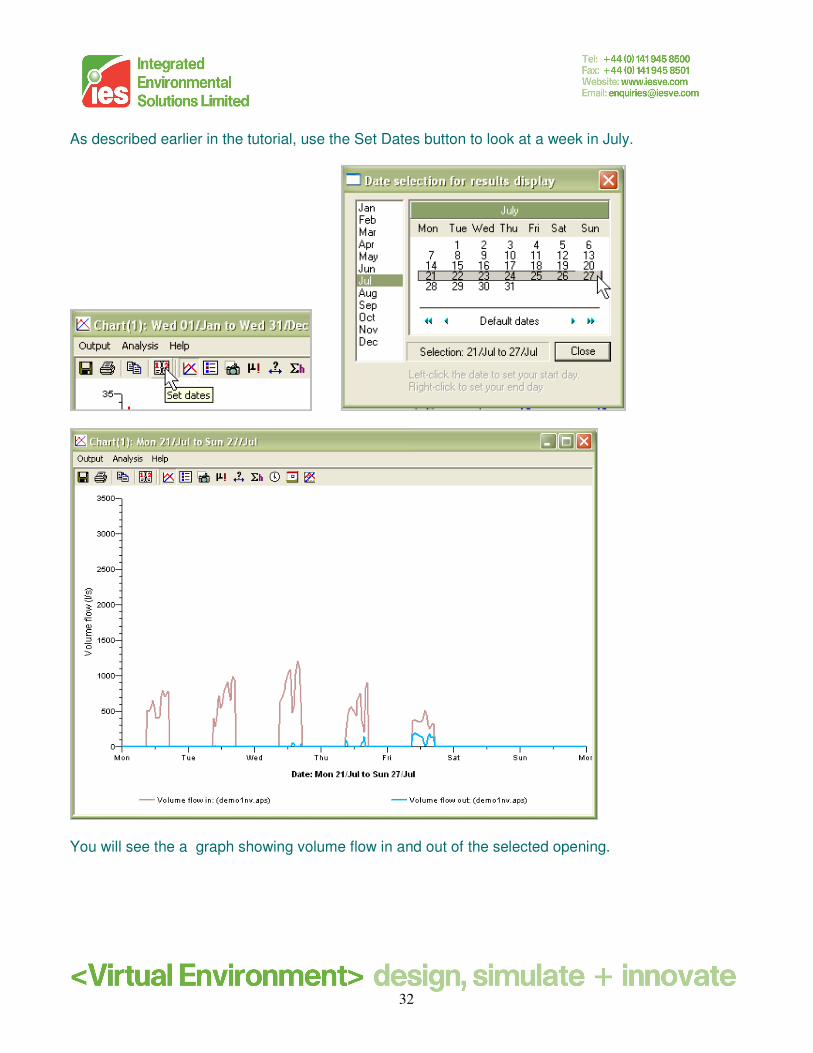
As described earlier in the tutorial, use the Set Dates button to look at a week in July.

You will see the a graph showing volume flow in and out of the selected opening.

33

If you wished, you could see a similar graph for the rooflight element you opened in the MacroFlo tutorial. You need to move up a level of decomposition, select the ceiling which contains the rooflight you opened, move down to the bottom level and select the rooflight that you opened. Close the graph. You have now completed the Vista tutorial.