ieee/acm transactions on audio, speech, …senarvi.github.io/publications/taslp2017.pdf ·...

IEEE/ACM TRANSACTIONS ON AUDIO, SPEECH, AND LANGUAGE PROCESSING, VOL. 25, NO. 11, NOVEMBER 2017 1

Automatic Speech Recognition with Very LargeConversational Finnish and Estonian Vocabularies

Seppo Enarvi, Peter Smit, Sami Virpioja, and Mikko Kurimo, Senior Member, IEEE

Abstract—Today, the vocabulary size for language models inlarge vocabulary speech recognition is typically several hundredsof thousands of words. While this is already sufficient in someapplications, the out-of-vocabulary words are still limiting theusability in others. In agglutinative languages the vocabulary forconversational speech should include millions of word forms tocover the spelling variations due to colloquial pronunciations, inaddition to the word compounding and inflections. Very largevocabularies are also needed, for example, when the recognitionof rare proper names is important.

Previously, very large vocabularies have been efficiently mod-eled in conventional n-gram language models either by splittingwords into subword units or by clustering words into classes.While vocabulary size is not as critical anymore in modern speechrecognition systems, training time and memory consumptionbecome an issue when state-of-the-art neural network languagemodels are used. In this paper we investigate techniques thataddress the vocabulary size issue by reducing the effective vocab-ulary size and by processing large vocabularies more efficiently.

The experimental results in conversational Finnish and Es-tonian speech recognition indicate that properly defined wordclasses improve recognition accuracy. Subword n-gram modelsare not better on evaluation data than word n-gram modelsconstructed from a vocabulary that includes all the words inthe training corpus. However, when recurrent neural network(RNN) language models are used, their ability to utilize longcontexts gives a larger gain to subword-based modeling. Ourbest results are from RNN language models that are based onstatistical morphs. We show that the suitable size for a subwordvocabulary depends on the language. Using time delay neuralnetwork (TDNN) acoustic models, we were able to achieve newstate of the art in Finnish and Estonian conversational speechrecognition, 27.1 % word error rate in the Finnish task and21.9 % in the Estonian task.

Index Terms—language modeling, word classes, subword units,artificial neural networks, automatic speech recognition

I. INTRODUCTION

F INNISH and Estonian are agglutinative languages, mean-ing that words are formed by concatenating smaller

linguistic units, and a great deal of grammatical informationis conveyed by inflection. Modeling these inflected wordscorrectly is important for automatic speech recognition, to pro-duce understandable transcripts. Recognizing a suffix correctlycan also help to predict the other words in the sentence. Bycollecting enough training data, we can get a good coverage of

Manuscript received January 31, 2017; revised July 7, 2017; accepted August7, 2017. This work was financially supported by the Academy of Finlandunder the grant numbers 251170 and 274075, and by Kone Foundation.

The authors work in the Department of Signal Processing and Acoustics atAalto University, Espoo, Finland. (e-mail: [email protected])

Digital Object Identifier 10.1109/TASLP.2017.2743344

the words in one form or another—perhaps names and numbersbeing an exception—but we are far from having enough trainingdata to find examples of all the inflected word forms.

Another common feature of Finnish and Estonian is thatthe orthography is phonemic. Consequently, the spelling of aword can be altered according to the pronunciation changes inconversational language. Especially Finnish conversations arewritten down preserving the variation that happens in colloquialpronunciation [1]. Modeling such languages as a sequence ofcomplete word forms becomes difficult, as most of the formsare very rare. In our data sets, most of the word forms appearonly once in the training data.

Agglutination has a far more limited impact on the vocab-ulary size in English. Nevertheless, the vocabularies used inEnglish language have grown as larger corpora are used andcomputers are able to store larger language models in memory.Moreover, as speech technology improves, we start to demandbetter recognition of e.g. proper names that do not appear inthe training data.

Modern automatic speech recognition (ASR) systems canhandle vocabularies as large as millions of words with simplen-gram language models, but a second recognition pass witha neural network language model (NNLM) is now necessaryfor achieving state-of-the-art performance. Vocabulary size ismuch more critical in NNLMs, as neural networks take along time to train, and training and inference times dependheavily on the vocabulary size. While computational efficiencyis the most important reason for finding alternatives to word-based modeling, words may not be the best choice of languagemodeling unit with regard to model performance either,especially when modeling agglutinative languages.

Subword models have been successfully used in FinnishASR for more than a decade [2]. In addition to reducing thecomplexity of the language model, subword models bringthe benefit that even words that do not occur in the trainingdata can be predicted. However, subwords have not been usedfor modeling conversational Finnish or Estonian before. Ourearlier attempts to use subwords for conversational FinnishASR failed to improve over word models. In this paper, weshow how subword models can be used in the FST-basedKaldi speech recognition toolkit and obtain the best resultsto date by rescoring subword lattices using subword NNLMs,27.1 % WER for spontaneous Finnish conversations, and 21.9% WER for spontaneous Estonian conversations. This is thefirst published evaluation of subwords in conversational Finnishand Estonian speech recognition tasks.

2329-9290 c© 2017 IEEE. Personal use is permitted, but republication/redistribution requires IEEE permission.See http://www.ieee.org/publications standards/publications/rights/index.html for more information.


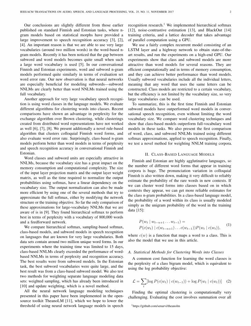
Our conclusions are slightly different from those earlierpublished on standard Finnish and Estonian tasks, where n-gram models based on statistical morphs have provided alarge improvement to speech recognition accuracy [3], [2],[4]. An important reason is that we are able to use very largevocabularies (around two million words) in the word-based n-gram models. Recently it has been noticed that the gap betweensubword and word models becomes quite small when sucha large word vocabulary is used [5]. In our conversationalFinnish and Estonian experiments, word and subword n-grammodels performed quite similarly in terms of evaluation setword error rate. Our new observation is that neural networksare especially beneficial for modeling subwords—subwordNNLMs are clearly better than word NNLMs trained using thefull vocabulary.

Another approach for very large vocabulary speech recogni-tion is using word classes in the language models. We evaluatedifferent algorithms for clustering words into classes. Recentcomparisons have shown an advantage in perplexity for theexchange algorithm over Brown clustering, while clusteringscreated from distributed word representations have not workedas well [6], [7], [8]. We present additionally a novel rule-basedalgorithm that clusters colloquial Finnish word forms, andalso evaluate word error rate. Surprisingly, class-based n-grammodels perform better than word models in terms of perplexityand speech recognition accuracy in conversational Finnish andEstonian.

Word classes and subword units are especially attractive inNNLMs, because the vocabulary size has a great impact on thememory consumption and computational complexity. The sizeof the input layer projection matrix and the output layer weightmatrix, as well as the time required to normalize the outputprobabilities using softmax, have a linear dependency on thevocabulary size. The output normalization can also be mademore efficient by using one of the several methods that try toapproximate the full softmax, either by modifying the networkstructure or the training objective. So far the only comparison ofthese approximations for large-vocabulary NNLMs that we areaware of is in [9]. They found hierarchical softmax to performbest in terms of perplexity with a vocabulary of 800,000 wordsand a feedforward network.

We compare hierarchical softmax, sampling-based softmax,class-based models, and subword models in speech recognitionon languages that are known for very large vocabularies. Bothdata sets contain around two million unique word forms. In ourexperiments where the training time was limited to 15 days,class-based NNLMs clearly exceeded the performance of word-based NNLMs in terms of perplexity and recognition accuracy.The best results were from subword models. In the Estoniantask, the best subword vocabularies were quite large, and thebest result was from a class-based subword model. We also testtwo methods for weighting separate language modeling datasets: weighted sampling, which has already been introduced in[10] and update weighting, which is a novel method.

All the neural network language modeling techniquespresented in this paper have been implemented in the open-source toolkit TheanoLM [11], which we hope to lower thethreshold of using neural network language models in speech

recognition research.1 We implemented hierarchical softmax[12], noise-contrastive estimation [13], and BlackOut [14]training criteria, and a lattice decoder that takes advantageof parallel computation using a GPU.

We use a fairly complex recurrent model consisting of anLSTM layer and a highway network to obtain state-of-the-art results, and run the experiments on a high-end GPU. Ourexperiments show that class and subword models are moreattractive than word models for several reasons. They areefficient computationally and in terms of memory consumption,and they can achieve better performance than word models.Usually subword vocabularies include all the individual letters,meaning that any word that uses the same letters can beconstructed. Class models are restricted to a certain vocabulary,but the efficiency is not limited by the vocabulary size, so verylarge vocabularies can be used.

To summarize, this is the first time Finnish and Estoniansubword models have outperformed word models in conver-sational speech recognition, even without limiting the wordvocabulary size. We compare word clustering techniques andshow that class-based models outperform full-vocabulary wordmodels in these tasks. We also present the first comparisonof word, class, and subword NNLMs trained using differentsoftmax approximations, applied to speech recognition. Finally,we test a novel method for weighting NNLM training corpora.

II. CLASS-BASED LANGUAGE MODELS

Finnish and Estonian are highly agglutinative languages, sothe number of different word forms that appear in trainingcorpora is huge. The pronunciation variation in colloquialFinnish is also written down, making it very difficult to reliablyestimate the probability of the rare words in new contexts. Ifwe can cluster word forms into classes based on in whichcontexts they appear, we can get more reliable estimates forthe class n-gram probabilities. In a class-based language model,the probability of a word within its class is usually modeledsimply as the unigram probability of the word in the trainingdata [15]:

P (wt | wt−n+1 . . . wt−1) =

P (c(wt) | c(wt−n+1) . . . c(wt−1))P (wt | c(wt)),(1)

where c(w) is a function that maps a word to a class. This isalso the model that we use in this article.

A. Statistical Methods for Clustering Words into Classes

A common cost function for learning the word classes isthe perplexity of a class bigram model, which is equivalent tousing the log probability objective:

L =∑t

[logP (c(wt) | c(wt−1)) + logP (wt | c(wt))] (2)

Finding the optimal clustering is computationally verychallenging. Evaluating the cost involves summation over all

1https://github.com/senarvi/theanolm


adjacent classes in the training data [15]. The algorithms thathave been proposed are suboptimal. Another approach thatcan be taken is to use knowledge about the language to groupwords that have a similar function.

Brown et al. [15] start by assigning each word to a distinctclass, and then merge classes in a greedy fashion. A naivealgorithm would evaluate the objective function for each pairof classes. One iteration of the naive algorithm would onaverage run in O(N4

V ) time, where NV is the size of thevocabulary. This involves a lot of redundant computation thatcan be eliminated by storing some statistics between iterations,reducing the time required to run one iteration to O(N2

V ).To further reduce the computational complexity, they propose

an approximation where, at any given iteration, only a subset ofthe vocabulary is considered. Starting from the most frequentwords, NC words are assigned to distinct classes. On eachiteration, the next word is considered for merging to one ofthe classes. The running time of one iteration is O(N2

C). Thealgorithm stops after NV − NC iterations, and results in allthe words being in one of the NC classes.

The exchange algorithm proposed by Kneser and Ney [16]starts from some initial clustering that assigns every word to oneof NC classes. The algorithm iterates through all the words inthe vocabulary, and evaluates how much the objective functionwould change by moving the word to each class. If there aremoves that would improve the objective function, the word ismoved to the class that provides the largest improvement.

By storing word and class bigram statistics, the evaluationof the objective function can be done in O(NC), and thus oneword iterated in O(N2

C) time [17]. The number of words thatwill be iterated is not limited by a fixed bound. Even thoughwe did not perform the experiments in such a way that wecould get a fair comparison of the training times, we noticedthat our exchange implementation needed less time to convergethan what the Brown clustering needed to finish.2

These algorithms perform a lot of computation of statisticsand evaluations over pairs of adjacent classes and words. Inpractice the running times are better than the worst caseestimates, because all classes and words do not follow eachother. The algorithms can also be parallelized using multipleCPUs, on the expense of memory requirements. Parallelizationusing a GPU would be difficult, because that would involvesparse matrices.

The exchange algorithm is greedy so the order in whichthe words are iterated may affect the result. The initializationmay also affect whether the optimization will get stuck ina local optimum, and how fast it will converge. We use theexchange3 tool, which by default initializes the classes bysorting the words by frequency and assigning word wi to classi mod NC , where i is the sorted index. We compare this toinitialization from other clustering methods.

2We are using a multithreaded exchange implementation and stop the trainingwhen the cost stops decreasing. Our observation that an optimized exchangeimplementation can be faster than Brown clustering is in line with an earliercomparison [6].

3https://github.com/aalto-speech/exchange

B. Clustering Based on Distributed Representation of Words

Neural networks that process words need to representthem using real-valued vectors. The networks learn the wordembeddings automatically. These distributed representationsare interesting on their own, because the network tends tolearn similar representation for semantically similar words [18].An interesting alternative to statistical clustering of words isto cluster words based on their vector representations usingtraditional clustering methods.

Distributed word representations can be created quicklyusing shallow networks, such as the Continuous Bag-of-Words(CBOW) model [19]. We use word2vec4 to cluster wordsby creating word embeddings using the CBOW model andclustering them using k-means.

C. A Rule-Based Method for Clustering Finnish Words

Much of the vocabulary in conversational Finnish textis due to colloquial Finnish pronunciations being writtendown phonetically. There are often several ways to write thesame word depending on how colloquial the writing styleis. Phonological processes such as reductions (“miksi” →“miks” [why]) and even word-internal sandhi (“menenpa” →“menempa” [I will go]) are often visible in written form.Intuitively grouping these different phonetic representationsof the same word together would provide a good clustering.While the extent to which a text is colloquial does providesome clues for predicting the next word, in many cases theseword forms serve exactly the same function.

This is closely related to normalization of imperfect text,a task which is common in all areas of language technology.Traditionally text normalization is based on hand-craftedrules and lookup tables. In the case that annotated data isavailable, supervised methods can be used for example toexpand abbreviations [20]. When annotations are not available,candidate expansions for a non-standard word can be foundby comparing its lexical or phonemic form to standard words[21]. The correct expansion often depends on the context. Alanguage model can be incorporated to disambiguate betweenthe alternative candidates when normalizing text. We are awareof one earlier work where colloquial Finnish has been translatedto standard Finnish using both rule-based normalization andstatistical machine translation [22].

Two constraints makes our task different from text nor-malization: A word needs to be classified in the same wayregardless of the context, and a word cannot be mapped to aword sequence. Our last clustering method, Rules, is based on aset of rules that describe the usual reductions and alternations incolloquial words. We iterate over a standard Finnish vocabularyand compare the standard Finnish word with every word in acolloquial Finnish vocabulary. If the colloquial word appears tobe a reduced pronunciation of the standard word, these wordsare merged into a class. Because all the words can appearin at most one class, multiple standard words can be mergedinto one class, but this is rare. Thus, there will be only ahandful of words in each class. Larger classes can be created

4https://code.google.com/archive/p/word2vec/


by merging the classes produced by this algorithm using someother clustering technique.

III. SUBWORD LANGUAGE MODELS

Subword modeling is another effective technique to reducevocabulary size. We use the Morfessor method [23], [24], whichhas been successfully applied in speech recognition of manyagglutinative languages [4], [25]. Morfessor is an unsupervisedmethod that uses a statistical model to split words into smallerfragments. As these fragments often resemble the surface formsof morphemes, the smallest information-bearing units of alanguage, we will use the term “morph” for them.

Morfessor has three components: a model, a cost function,and the training and decoding algorithm. The model consists ofa lexicon and a grammar. The lexicon contains the propertiesof the morphs, such as their written forms and frequencies.The grammar contains information of how the morphs can becombined into words. The Morfessor cost function is derivedfrom MAP estimation with the goal of finding the optimalparameters θ given the observed training data DW :

θMAP = argmaxθ

P (θ | DW )

= argmaxθ

P (θ)P (DW | θ)(3)

The objective function to be maximized is the logarithm ofthe product P (θ)P (DW | θ). In a semisupervised setting, it isuseful to add a hyperparameter to control the weight of thedata likelihood [26]:

L(θ,DW ) = logP (θ) + α logP (DW | θ) (4)

We use the hyperparameter α to control the degree ofsegmentation in a heuristic manner. This allows for optimizingthe segmentation, either for optimal perplexity or speechrecognition accuracy or to obtain a specific size lexicon. Agreedy search algorithm is used to find the optimal segmentationof morphs, given the training data. When the best model isfound, it is used to segment the language model training corpususing the Viterbi algorithm.

We apply the Morfessor 2.0 implementation5 of the Mor-fessor Baseline algorithm with the hyperparameter extension[27]. In the output segmentation, we prepend and appendthe in-word boundaries of the morph surface forms by a “+”character. For example the compound word “luentokalvoja”is segmented into “luento kalvo ja” and then transformed to“luento+ +kalvo+ +ja” [lecture+ +slide+ +s] before languagemodel training. All four different variants of a subword (e.g.“kalvo”, “kalvo+”, “+kalvo”, and “+kalvo+”) are treated asseparate tokens in language model training. As high-ordern-grams are required to provide enough context informationfor subword-based modeling, we use variable-length n-grammodels trained using the VariKN toolkit6 that implements theKneser-Ney growing and revised Kneser pruning algorithms[28].

5https://github.com/aalto-speech/morfessor6https://github.com/vsiivola/variKN

In the speech recognition framework based on weightedfinite-state transducers (FSTs), we restrict the lexicon FST insuch a way that only legal sequences (meaning that a morphcan start with “+” if and only if the previous morph ends witha “+”) are allowed [29]. After decoding the ASR results, themorphs are joined together to form words for scoring.

IV. NEURAL NETWORK LANGUAGE MODELS

Recurrent neural networks are known to work well for mod-eling language, as they can capture the long-term dependenciesneglected by n-gram models [30]. Especially the subword-basedapproach should benefit from this capability of modeling longcontexts. In this article we experiment with language modelsthat are based on LSTMs and highway networks. These arelayer types that use sigmoid gates to control information flow.The gates are optimized along with the rest of the neuralnetwork parameters, and learn to pass the relevant activationsover long distances.

LSTM [31] is a recurrent layer type. Each gate can be seenas an RNN layer with two weight matrices, W and U , a biasvector b, and sigmoid activation. The output of a gate at timestep t is

g(xt, ht−1) = σ(Wxt + Uht−1 + b), (5)

where xt is the output vector of the previous layer and ht−1is the LSTM layer state vector from the previous time step.When a signal is multiplied by the output of a sigmoid gate,the system learns to discard unimportant elements of the vectordepending on the gate’s input.

An LSTM layer uses three gates to select what informationto pass from the previous time step to the next time stepunmodified, and what information to modify. The same ideacan be used to select what information to pass to the next layer.Highway networks [32] use gates to facilitate information flowacross many layers. At its simplest, only one gate is needed.In the feedforward case, there is only one input, xt, and thegate needs only one weight matrix, Wσ. The gate learns toselect between the layer’s input and its activation:

g(xt) = σ(Wσxt + bσ)

yt = g(xt)� tanh(Wxt + b) + (1− g(xt))� xt(6)

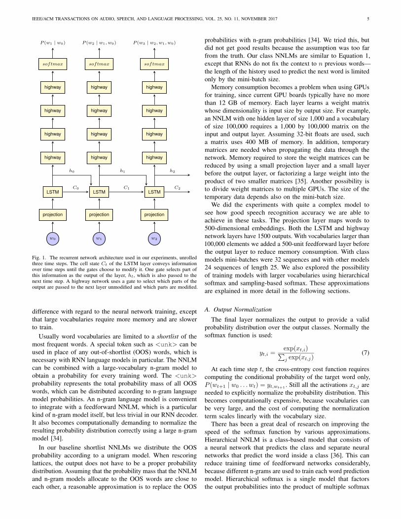
While LSTM helps propagation of activations and gradientsin recurrent networks, deep networks benefit from highwayconnections. We did not notice much improvement by stackingmultiple LSTM layers on top of each other. While we did nothave the possibility to systematically explore different networkarchitectures, one LSTM layer followed by a highway networkseemed to perform well. The architecture used in this articleis depicted in Figure 1. Every layer was followed by Dropout[33] at rate 0.2.

The input of the network at time step t is wt, an indexthat identifies the vocabulary element. The output containsthe predicted probabilities for every vocabulary element, butonly the output corresponding to the target word is used. Thevocabulary can consist of words, word classes, subwords, orsubword classes. The choice of vocabulary does not make any


P (w1 | w0) P (w2 | w1, w0) P (w3 | w2, w1, w0)

softmax softmax softmax

highway highway highway




LSTM LSTM LSTM

projection projection projection

w0 w1 w2

C0 C1 C2

h0 h1 h2

Fig. 1. The recurrent network architecture used in our experiments, unrolledthree time steps. The cell state Ct of the LSTM layer conveys informationover time steps until the gates choose to modify it. One gate selects part ofthis information as the output of the layer, ht, which is also passed to thenext time step. A highway network uses a gate to select which parts of theoutput are passed to the next layer unmodified and which parts are modified.

difference with regard to the neural network training, exceptthat large vocabularies require more memory and are slowerto train.

Usually word vocabularies are limited to a shortlist of themost frequent words. A special token such as <unk> can beused in place of any out-of-shortlist (OOS) words, which isnecessary with RNN language models in particular. The NNLMcan be combined with a large-vocabulary n-gram model toobtain a probability for every training word. The <unk>probability represents the total probability mass of all OOSwords, which can be distributed according to n-gram languagemodel probabilities. An n-gram language model is convenientto integrate with a feedforward NNLM, which is a particularkind of n-gram model itself, but less trivial in our RNN decoder.It also becomes computationally demanding to normalize theresulting probability distribution correctly using a large n-grammodel [34].

In our baseline shortlist NNLMs we distribute the OOSprobability according to a unigram model. When rescoringlattices, the output does not have to be a proper probabilitydistribution. Assuming that the probability mass that the NNLMand n-gram models allocate to the OOS words are close toeach other, a reasonable approximation is to replace the OOS

probabilities with n-gram probabilities [34]. We tried this, butdid not get good results because the assumption was too farfrom the truth. Our class NNLMs are similar to Equation 1,except that RNNs do not fix the context to n previous words—the length of the history used to predict the next word is limitedonly by the mini-batch size.

Memory consumption becomes a problem when using GPUsfor training, since current GPU boards typically have no morethan 12 GB of memory. Each layer learns a weight matrixwhose dimensionality is input size by output size. For example,an NNLM with one hidden layer of size 1,000 and a vocabularyof size 100,000 requires a 1,000 by 100,000 matrix on theinput and output layer. Assuming 32-bit floats are used, sucha matrix uses 400 MB of memory. In addition, temporarymatrices are needed when propagating the data through thenetwork. Memory required to store the weight matrices can bereduced by using a small projection layer and a small layerbefore the output layer, or factorizing a large weight into theproduct of two smaller matrices [35]. Another possibility isto divide weight matrices to multiple GPUs. The size of thetemporary data depends also on the mini-batch size.

We did the experiments with quite a complex model tosee how good speech recognition accuracy we are able toachieve in these tasks. The projection layer maps words to500-dimensional embeddings. Both the LSTM and highwaynetwork layers have 1500 outputs. With vocabularies larger than100,000 elements we added a 500-unit feedforward layer beforethe output layer to reduce memory consumption. With classmodels mini-batches were 32 sequences and with other models24 sequences of length 25. We also explored the possibilityof training models with larger vocabularies using hierarchicalsoftmax and sampling-based softmax. These approximationsare explained in more detail in the following sections.

A. Output Normalization

The final layer normalizes the output to provide a validprobability distribution over the output classes. Normally thesoftmax function is used:

yt,i =exp(xt,i)∑j exp(xt,j)

(7)

At each time step t, the cross-entropy cost function requirescomputing the conditional probability of the target word only,P (wt+1 | w0 . . . wt) = yt,wt+1

. Still all the activations xt,j areneeded to explicitly normalize the probability distribution. Thisbecomes computationally expensive, because vocabularies canbe very large, and the cost of computing the normalizationterm scales linearly with the vocabulary size.

There has been a great deal of research on improving thespeed of the softmax function by various approximations.Hierarchical NNLM is a class-based model that consists ofa neural network that predicts the class and separate neuralnetworks that predict the word inside a class [36]. This canreduce training time of feedforward networks considerably,because different n-grams are used to train each word predictionmodel. Hierarchical softmax is a single model that factorsthe output probabilities into the product of multiple softmax


functions. The idea has originally been used in maximumentropy training [12], but exactly the same idea can be appliedto neural networks [37]. SOUL combines a shortlist for themost frequent words with hierarchical softmax for the out-of-shortlist words [38]. Adaptive softmax [39] is a similarapproach that optimizes the word cluster sizes to minimizecomputational cost on GPUs.

Another group of methods do not modify the model, butuse sampling during training to approximate the expensivesoftmax normalization. These methods speed up training, butuse normal softmax during evaluation. Importance sampling isa Monte Carlo method that samples words from a distributionthat should be close to the network output distribution [40].Noise-contrastive estimation (NCE) samples random words, butinstead of optimizing the cross-entropy cost directly, it uses anauxiliary cost that learns to classify a word as a training wordor a noise word [13]. This allows it to treat the normalizationterm as a parameter of the network. BlackOut continues thisline of research, using a stochastic version of softmax thatexplicitly discriminates the target word from the noise words[14].

Variance regularization modifies the training objective toencourage the network to learn an output distribution that isclose to a real probability distribution even without explicitnormalization [41]. This is useful for example in one-passspeech recognition, where evaluation speed is important butthe output does not have to be a valid probability distribution.The model can also be modified to predict the normalizationterm along with the word probabilities [42]. NCE objective alsoencourages the network to learn an approximately normalizeddistribution, and can also be used without softmax e.g. forspeech recognition [43].

B. Hierarchical Softmax

Hierarchical softmax factors the output probabilities intothe product of multiple softmax functions. At one extreme,the hierarchy can be a balanced binary tree that is log2(N)levels deep, where N is the vocabulary size. Each level woulddifferentiate between two classes, and in total the hierarchicalsoftmax would take logarithmic time. [37]

We used a two-level hierarchy, because it is simple toimplement, and it does not require a hierarchical clusteringof the vocabulary. The first level performs a softmax between√N word classes and the second level performs a softmax

between√N words inside the correct class:

P (wt | w0 . . . wt−1) =

P (c(wt) | w0 . . . wt−1)P (wt | w0 . . . wt−1, c(wt))(8)

This already reduces the time complexity of the output layerto the square root of the vocabulary size.

The clustering affects the performance of the resulting model,but it is not clear what kind of clustering is optimal for thiskind of models. In earlier work, clusterings have been createdfrom word frequencies [44], by clustering distributed wordrepresentations [45], and using expert knowledge [37].

Ideally all class sizes would be equal, as the matrix productthat produces the preactivations can be computed efficiently

on a GPU when the weight matrix is dense. We use the sameword classes in the hierarchical softmax layer that we usein class-based models, but we force equal class sizes; afterrunning the clustering algorithm, we sort the vocabulary byclass and split it into partitions of size

√N . This may split

some classes unnecessarily into two, which is not optimal. Onthe other hand it is easy to implement and even as simplemethods as frequency binning seem to work [44].

An advantage of hierarchical softmax compared to samplingbased output layers is that hierarchical softmax speeds upevaluation as well, while sampling is used only during trainingand the output is properly normalized using softmax duringinference.

C. Sampling-Based Approximations of Softmax

Noise-contrastive estimation [13] turns the problem fromclassification between N words into binary classification. Foreach training word, a set of noise words (one in the originalpaper) is sampled from some simple distribution. The networklearns to discriminate between training words and noise words.The binary-valued class label Cw is used to indicate whetherthe word w is a training or noise word. The authors derivethe probability that an arbitrary word comes from either class,P (Cw | w), given the probability distributions of both classes.The objective function is the cross entropy of the binaryclassifier:

L =∑w

[Cw logP (Cw = 1 | w)

+ (1− Cw) logP (Cw = 0 | w)](9)

The expensive softmax normalization can be avoided bymaking the normalization term a network parameter that islearned along the weights during training. In a language model,the parameter would be dependent on the context words, but itturns out that it can be fixed to a context-independent constantwithout harming the performance of the resulting model [46].In the beginning of the training the cost will be high andthe optimization may be unstable, unless the normalizationis close to correct. We use one as the normalization constantand initialize the output layer bias to the logarithmic unigramdistribution, so that in the beginning the network correspondsto the maximum likelihood unigram distribution.

BlackOut [14] is also based on sampling a set of noisewords, and motivated by the discriminative loss of NCE, but theobjective function directly discriminates between the trainingword wT and noise words wN :

L =∑wT

[logP (wT ) +∑wN

log(1− P (wN ))] (10)

Although not explicitly shown, the probabilities P (w) areconditioned on the network state. They are computed using aweighted softmax that is normalized only on the set of trainingand noise words. In addition to reducing the computation, thiseffectively performs regularization in the output layer similarlyto how the Dropout [33] technique works in the hidden layers.

Often the noise words are sampled from the uniformdistribution, or from the unigram distribution of the words


in the training data [46]. Our experiments confirmed that thechoice of proposal distribution is indeed important. Usinguniform distribution, the neural network optimization will notfind as good parameters. With unigram distribution the problemis that some words may be sampled very rarely. Mikolov et al.[47] use the unigram distribution raised to the power of β. Jiet al. [14] make β a tunable parameter. They also exclude thecorrect target words from the noise distribution.

We used the power distribution with β = 0.5 for bothBlackOut and NCE. We did not modify the distribution basedon the target words, however, as that would introduce additionalmemory transfers by the Theano computation library used byTheanoLM. We observed also that random sampling from amultinomial distribution in Theano does not work as efficientlyas possible with a GPU. We used 500 noise words, sharedacross the mini-batch. These values were selected after notingthe speed of convergence with a few values. Small β valuesflatten the distribution too much and the optimal model isnot reached. Higher values approach the unigram distribution,causing the network to not learn enough about the rare words.Using more noise words makes mini-batch updates slower,while using only 100 noise words we noticed that the trainingwas barely converging.

These methods seem to suffer from some disadvantages.Properly optimizing the β parameter can take a considerableamount of time. A large enough set of noise words has tobe drawn for the training to be stable, diminishing the speedadvantage in our GPU implementation. While we did try anumber of different parameter combinations, BlackOut neverfinished training on these data sets without numerical errors.

D. Decoding Lattices with RNN Language ModelsWhile improving training speed is the motivation behind

the various softmax approximations, inference is also slow onlarge networks. Methods that modify the network structure,such as hierarchical softmax, improve inference speed as well.Nevertheless, using an RNN language model in the first pass oflarge-vocabulary speech recognition is unrealistic. It is possibleto create a list of n best hypothesis, or a word lattice, during thefirst pass, and rescore them using an NNLM in a second pass.We have implemented a word lattice decoder in TheanoLMthat produces better results than rescoring n-best lists.

Conceptually, the decoder propagates tokens through thelattice. Each token stores a network state and the probabilityof the partial path. At first one token is created at the startnode with the initial network state. The algorithm iterates bypropagating tokens to the outgoing links of a node, creatingnew copies of the tokens for each link. Evaluating a singleword probability at a time would be inefficient, so the decodercombines the state from all the tokens in the node into a matrix,and the input words into another matrix. Then the network isused to simultaneously compute the probability of the targetword in all of these contexts.

Rescoring a word lattice using an RNN language modelis equivalent to rescoring a huge n-best list, unless someapproximation is used to limit the dependency of a probabilityon the earlier context. We apply three types of pruning, beforepropagation, to the tokens in the node [48]:

• n-gram recombination. If there are multiple tokens,whose last n context words match, keep only the best.We use n = 22.

• cardinality pruning. Keep at most c best tokens. Weuse c = 62.

• beam pruning. Prune tokens whose probability is low,compared to the best token. The best token is searchedfrom all nodes that appear at the same time instance, orin the future. (Tokens in the past have a higher probabilitybecause they correspond to a shorter time period.) Weprune tokens if the difference in log probability is largerthan 650.

We performed a few tests with different pruning parametersand chose large enough n and c so that their effect in the resultswas negligible. Using a larger beam would have improved theresults, but the gain would have been small compared to theincrease in decoding time.

V. EXPERIMENTS

A. Data Sets

We evaluate the methods on difficult spontaneous Finnishand Estonian conversations. The data sets were created in asimilar manner for both languages. For training acoustic modelswe combined spontaneous speech corpora with other less spon-taneous language that benefits acoustic modeling. For traininglanguage models we combined transcribed conversations withweb data that has been filtered to match the conversationalspeaking style [49].

For the Finnish acoustic models we used 85 hours of trainingdata from three sources. The first is the complete FinnishSPEECON [50] corpus. This corpus includes 550 speakersin different noise conditions that all have read 30 sentencesand 30 words, numbers, or dates, and spoken 10 spontaneoussentences. Two smaller data sets of better matching spontaneousconversations were used: DSPCON [51] corpus, which consistsof short conversations between Aalto University students, andFinDialogue part of the FinINTAS [52] corpus, which containslonger spontaneous conversations. For language modeling weused 61,000 words from DSPCON and 76 million words ofweb data. We did not differentiate between upper and lowercase. This resulted in 2.4 million unique words.

For the Estonian acoustic models we used 164 hours oftraining data, including 142 hours of broadcast conversations,news, and lectures collected at Tallinn University of Technology[53], and 23 hours of spontaneous conversations collected atthe University of Tartu7. These transcripts contain 1.3 millionwords. For language modeling we used additionally 82 millionwords of web data. The language model training data contained1.8 million unique words, differentiating between upper andlower case. One reason why the Estonian vocabulary is smallerthan the Finnish vocabulary, even though the Estonian data set islarger, is that colloquial Estonian is written in a more systematicway. Also standard Estonian vocabulary is smaller than standardFinnish vocabulary [25], probably because standard Finnishuses more inflected word forms.

7Phonetic Corpus of Estonian Spontaneous Speech. For information ondistribution, see http://www.keel.ut.ee/et/foneetikakorpus.


TABLE IOut-of-vocabulary word rates (%) of the evaluation sets, excluding start andend of sentence tokens. The last row is the full training set vocabulary, which

applies also for the class models.

Vocabulary Size Finnish Estonian100,000 6.67 3.89500,000 3.36 1.592.4M (Fin) / 1.8M (Est) 2.31 1.01

We use only spontaneous conversations as developmentand evaluation data. As mentioned earlier, Finnish words canbe written down in as many different ways as they can bepronounced in colloquial speech. When calculating Finnishword error rates we accept the different forms of the sameword as correct, as long as they could be used in the particularcontext. Compound words are accepted even if they are writtenas separate words. However, we compute perplexities ontranscripts that contain the phonetically verbatim word forms,excluding out-of-vocabulary (OOV) words. The perplexitiesfrom n-gram and neural network word and class models areall comparable to one another, because they model the samevocabulary consisting of all the training set words. Subwordscan model also unseen words, so the perplexities in subwordexperiments are higher. OOV word rates of the evaluation setsare reported in Table I for different vocabulary sizes.

The Estonian web data is the filtered data from [49]. Thesame transcribed data is also used, except that we removedfrom the acoustic training set three speakers that appear in theevaluation set. The evaluation data is still 1236 sentences or 2.9hours. The Finnish data is what we used in [11], augmentedwith 2016 data of DSPCON and read speech from SPEECON.While we now have more than doubled the amount of acoustictraining data, we have only a few more hours of spontaneousconversations. The switch to neural network acoustic modelshad a far greater impact on the results than the additionaltraining data. We still use the same Finnish evaluation setof 541 sentences or 44 minutes. The Finnish developmentand evaluation sets and reference transcripts that contain thealternative forms are included in the latest DSPCON release,without a few sentences that we could not license.

B. Models

The word based n-gram models were 4-grams, trained usingthe Modified Kneser-Ney implementation of SRILM toolkit[54]. Class-based models did not use Kneser-Ney smoothing,because the class n-gram statistics were not suitable forcomputing the Modified Kneser-Ney discount parameters. Thequality of our web data is very different from the transcribedconversations, and simply pooling all the training data togetherwould cause the larger web data to dominate the model.Instead we created separate models from different data sets,and combined them by interpolating the probabilities of theobserved n-grams from the component models using weightsthat were optimized on the development data. In the Finnishtask we created a mixture from two models, a web datamodel and a transcribed data model. In the Estonian task we

created a mixture from three models, separating the transcribedspontaneous conversations from the broadcast conversations.

The mixture weights were optimized independently for eachlanguage model on the development data, using expectationmaximization (EM). In the Finnish experiments this gave thetranscribed data a weight slightly less than 0.5. In the Estonianexperiments the weights of the spontaneous conversations andthe web data were typically around 0.4, while the broadcastswere given a weight less than 0.2. Morph models were similarlycombined from component models, but the EM optimizationfailed to give good weights. We used initially those optimizedfor the word-based models, and after the other parameters werefixed, we optimized the mixture weights for development setperplexity using a grid search with steps of 0.05.

The word clustering algorithms do not support training dataweighting, so we simply concatenated the data sets. There aremany parameters that can be tweaked when creating distributedword representations with word2vec. We tried clustering wordsusing a few different parameters, and report only the best n-gram model for each class vocabulary size. Within the set ofvalues that we tried, the best performance was obtained withcontinuous bag of words (CBOW), window size 8, and layersize 300 to 500.

For the subword language models, we trained Morfessor on aword list combined from all training corpora; the difference toother options such as token-based training was negligible. Foreach language, four segmentations were trained with α-values0.05, 0.2, 0.5, and 1.0. This resulted in respective vocabularysizes of 42.5k, 133k, 265k, and 468k for Finnish, and 33.2k,103k, 212k, and 403k for Estonian. The sizes include thedifferent morph variants with “+” prefix and affix. Whentraining the subword n-gram models with the VariKN toolkit,the growing threshold was optimized on the development set,while keeping the pruning threshold twice as large as thegrowing threshold.

Word-based neural network models were trained on twoshortlist sizes: 100k and 500k words. With 500k wordswe added a normal 500-unit layer with hyperbolic tangentactivation before the output layer, which reduced memoryconsumption and speeded up training. The neural networkswere trained using Adagrad [55] optimizer until convergenceor until the maximum time limit of 15 days was reached. Allneural network models were trained on a single NVIDIA TeslaK80 GPU and the training times were recorded.

We tried two different approaches for weighting the differentdata sets during neural network training: by randomly samplinga subset of every data set in the beginning of each epoch[10], and by weighting the parameter updates depending onfrom which corpus each sentence comes from. In the latterapproach, the gradient is scaled by both the learning rate and aconstant that is larger for higher-quality data, before updatingthe parameters. We are not aware that this kind of updateweighting would have been used before.

Optimizing the weights for neural network training is moredifficult than for the n-gram mixture models. As we do not havea computational method for optimizing the weights, we trieda few values, observing the development set perplexity duringtraining. Sampling 20 % of the web data on each iteration,


or weighting the web data by a factor of 0.4 seemed to workreasonably well. We used a slightly higher learning rate whenweighting the web data to compensate for the fact that theupdates are smaller on average. More systematic tests wereperformed using these weights with the five vocabularies inTable III.

It would be possible to train separate neural network modelsfrom each data set, but there are no methods for mergingseveral neural networks in the similar fashion that we combinethe n-gram models. Often the best possible NNLM results areobtained by interpolating probabilities from multiple models,but that kind of system is cumbersome in practice, requiringmultiple models to be trained and used for inference. The layersizes and other parameters would have to be optimized foreach model separately.

We combined the NNLMs with the nonclass word orsubword n-gram model by log-linear interpolation. We didnot notice much difference to linear interpolation, so we choseto do the interpolation in logarithmic space, because the wordprobabilities may be smaller than what can be represented using64-bit floats. We noticed that optimization of the interpolationparameters was quite difficult with our development data, sowe gave equal weight to both models. In some cases it couldhave been beneficial to give a larger weight to the neuralnetwork model. Development data was used to select a weightfor combining language model and acoustic scores from fourdifferent values.

C. Speech Recognition SystemWe use the Kaldi [56] speech recognition system for training

our acoustic models and for first-pass decoding. The TDNNacoustic models were trained on a pure sequence criterionusing Maximum Mutual Information (MMI) [57]. The datasets were cleaned and filtered using a Gaussian MixtureModel recognizer and augmented through speed and volumeperturbation [58]. The number of layers and parameters of theTDNN were optimized to maximize development set accuracyon the word model. First-pass decoding was very fast withreal-time factor less than 0.5. The accuracy of the first-passrecognition exceeded our earlier results on both data sets [11],[49], due to the new neural network acoustic models.

Kaldi does not, at this moment, directly support class-based decoding. Instead we created lattices using regularn-gram models, and rescored them with class n-gram andneural network models. Using the methods described in [59]it is possible to construct a word FST that represents theprobabilities of a class-based language model and use this infirst-pass decoding or rescoring, without explicitly using theclasses. Kaldi does not have any restrictions on vocabularysize, but compiling the FST-based decoding graph from thelanguage model, pronunciation dictionary, context dependencyinformation, and HMM structure did consume around 60 GB ofmemory. The memory requirement can be lowered by reducingthe number of contexts in the first-pass n-gram model.

D. ResultsTable II lists perplexities and word error rates given by n-

gram language models on the development data. The baseline

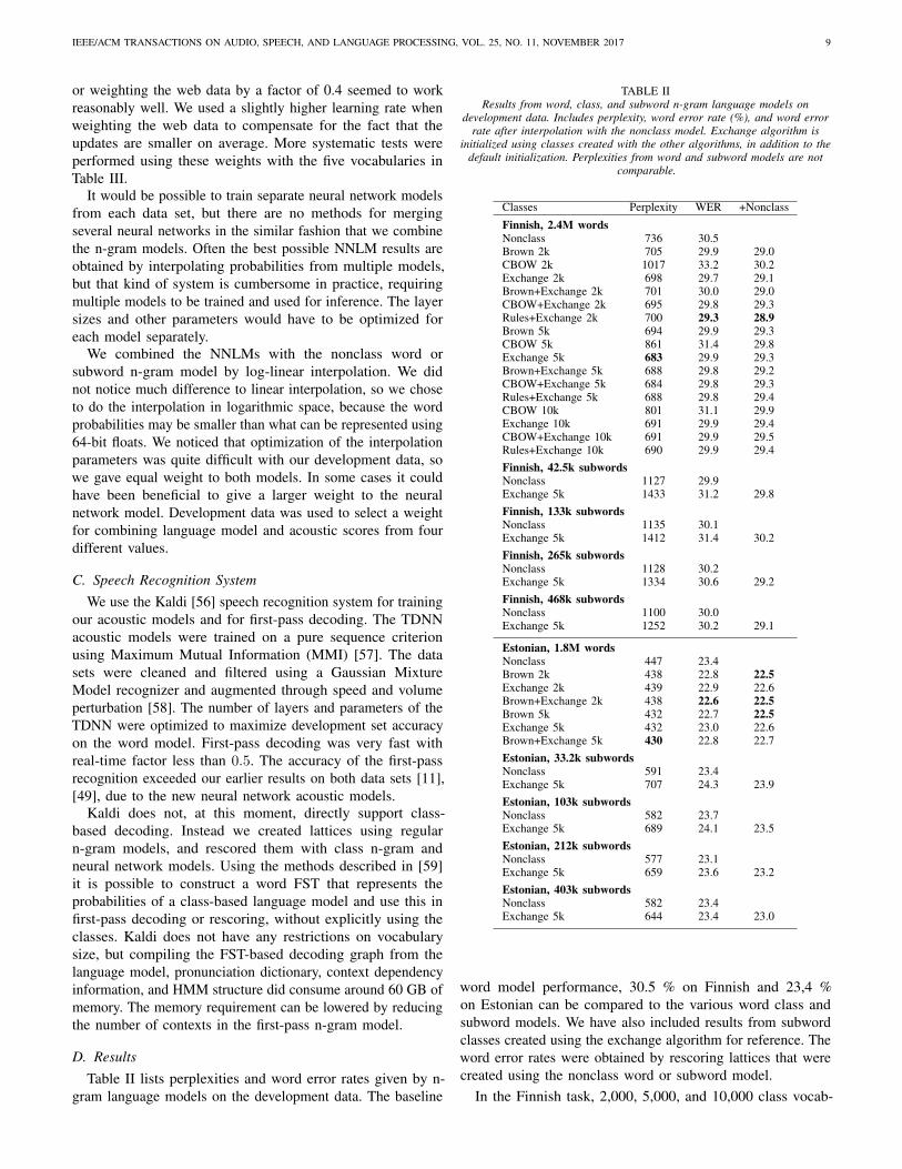
TABLE IIResults from word, class, and subword n-gram language models on

development data. Includes perplexity, word error rate (%), and word errorrate after interpolation with the nonclass model. Exchange algorithm is

initialized using classes created with the other algorithms, in addition to thedefault initialization. Perplexities from word and subword models are not

comparable.

Classes Perplexity WER +Nonclass

Finnish, 2.4M wordsNonclass 736 30.5Brown 2k 705 29.9 29.0CBOW 2k 1017 33.2 30.2Exchange 2k 698 29.7 29.1Brown+Exchange 2k 701 30.0 29.0CBOW+Exchange 2k 695 29.8 29.3Rules+Exchange 2k 700 29.3 28.9Brown 5k 694 29.9 29.3CBOW 5k 861 31.4 29.8Exchange 5k 683 29.9 29.3Brown+Exchange 5k 688 29.8 29.2CBOW+Exchange 5k 684 29.8 29.3Rules+Exchange 5k 688 29.8 29.4CBOW 10k 801 31.1 29.9Exchange 10k 691 29.9 29.4CBOW+Exchange 10k 691 29.9 29.5Rules+Exchange 10k 690 29.9 29.4Finnish, 42.5k subwordsNonclass 1127 29.9Exchange 5k 1433 31.2 29.8Finnish, 133k subwordsNonclass 1135 30.1Exchange 5k 1412 31.4 30.2Finnish, 265k subwordsNonclass 1128 30.2Exchange 5k 1334 30.6 29.2Finnish, 468k subwordsNonclass 1100 30.0Exchange 5k 1252 30.2 29.1

Estonian, 1.8M wordsNonclass 447 23.4Brown 2k 438 22.8 22.5Exchange 2k 439 22.9 22.6Brown+Exchange 2k 438 22.6 22.5Brown 5k 432 22.7 22.5Exchange 5k 432 23.0 22.6Brown+Exchange 5k 430 22.8 22.7Estonian, 33.2k subwordsNonclass 591 23.4Exchange 5k 707 24.3 23.9Estonian, 103k subwordsNonclass 582 23.7Exchange 5k 689 24.1 23.5Estonian, 212k subwordsNonclass 577 23.1Exchange 5k 659 23.6 23.2Estonian, 403k subwordsNonclass 582 23.4Exchange 5k 644 23.4 23.0

word model performance, 30.5 % on Finnish and 23,4 %on Estonian can be compared to the various word class andsubword models. We have also included results from subwordclasses created using the exchange algorithm for reference. Theword error rates were obtained by rescoring lattices that werecreated using the nonclass word or subword model.

In the Finnish task, 2,000, 5,000, and 10,000 class vocab-


ularies were compared. The worst case running times of theexchange and Brown algorithms have quadratic dependencyon the number of classes. With 10,000 classes, even using 20CPUs Brown did not finish in 20 days, so the experiment wasnot continued. The exchange algorithm can be stopped anytime, so there is no upper limit on the number of classes thatcan be trained, but the quality of the clustering may sufferif it is stopped early. However, with 5,000 classes and usingonly 5 CPUs, it seemed to converge in 5 days. Increasing thenumber of threads increases memory consumption. Trainingeven 40,000 classes was possible in 15 days, but the resultsdid not improve, so they are not reported. The most promisingmodels were evaluated also in the Estonian task.

CBOW is clearly the fastest algorithm, which is probablywhy it has gained some popularity. These results show, however,that the clusters formed by k-means from distributed wordrepresentations are not good for n-gram language models.CBOW does improve, compared to the other clusterings,when the number of classes is increased. Other than that, thedifferences between different classification methods are mostlyinsignificant, but class-based models outperform word modelson both languages. This result suggests that class-based softmaxmay be a viable alternative to other softmax approximationsin neural networks. The performance of the Estonian subwordmodels is close to that of the word model, and the Finnishsubword models are better than the word model. Subwordclasses do not work as well, but the difference to nonclasssubword models gets smaller when the size of the subwordvocabulary increases.

Mostly the differences between the different initializations ofthe exchange algorithm seemed insignificant. However, our rule-based clustering algorithm followed by running the exchangealgorithm to create 2,000 classes (Rules+Exchange 2k) gavethe best word error rate on Finnish. In the NNLM experimentswe did not explore with different clusterings, but used the onesthat gave the smallest development set perplexity in the n-gramexperiments. For Finnish the 5,000 classes created using theexchange algorithm was selected (Exchange 5k). On Estonian,initialization using Brown classes gave slightly better perplexity(Brown+Exchange 5k) and was selected for neural networkmodels.

Table III compares training time, perplexity, and word errorrate in NNLM training, when different processing is appliedto the large web data set. Uniform means that the web datais processed just like other data sets, sampling means that asubset of web data is randomly sampled before each epoch,and weighting means that the parameter updates are given asmaller weight when the mini-batch contains web sentences.Sampling seems to improve perplexity, but not word errorrate. Because sampling usually speeds up training considerablyand our computational resources were limited, the rest of theexperiments were done using sampling.

Table IV lists perplexities and word error rates given byneural network models on the development data. The word errorrates were obtained by rescoring the same lattices as in Table II.The shortlist and word class models can predict all training setwords, so the perplexities can be compared. Subword modelscan predict also new words, so their perplexities cannot be

TABLE IIIComparison of uniform data processing, random sampling of web data by

20 %, and weighted parameter updates from web data by a factor of 0.4, inNNLM training. The models were trained using normal softmax. Includesdevelopment set perplexity, word error rate (%), and word error rate after

interpolation with the n-gram model.

Subset TrainingProcessing Time Perplexity WER +NGram

Finnish, 5k classesUniform 143 h 511 26.0 25.6Sampling 128 h 505 26.2 25.6Weighting 101 h 521 26.4 25.5Finnish, 42.5k subwordsUniform 360 h 679 25.2 24.6Sampling 360 h 671 25.5 25.0Weighting 360 h 672 25.1 24.6Finnish, 468k subwords, 5k classesUniform 141 h 790 26.0 25.0Sampling 119 h 761 25.9 25.1

Estonian, 5k classesUniform 86 h 339 19.8 19.9Sampling 87 h 311 20.2 19.9Weighting 105 h 335 20.0 19.6Estonian, 212k subwords, 5k classesUniform 187 h 424 20.0 19.7Sampling 130 h 397 20.0 19.8Weighting 187 h 409 19.9 19.6

compared with word models. The percentage of evaluation setwords that are not in the shortlist and words that are not inthe training set can be found in Table I.

The class-based models were clearly the fastest to converge,5 to 8 days on Finnish data and 4 to 6 days on Estoniandata. The experiments include shortlists of 100k and 500kwords. Other shortlist models, except the Estonian 100k-wordNCE, did not finish before the 360 hour limit. Consequently,improvement was not seen from using a larger 500k-wordshortlist.

Our NCE implementation required more GPU memory thanhierarchical softmax and we were unable to run it with thelarger shortlist. With the smaller shortlist NCE was better onFinnish and hierarchical softmax was better on Estonian. Weexperienced issues with numerical stability using NCE withsubwords, and decided to use only hierarchical softmax in thesubword experiments. BlackOut training was slightly fasterthan NCE, but even less stable, and we were unable to finishthe training without numerical errors. With hierarchical softmaxwe used the same classes that were used in the class-basedmodels, but the classes were rearranged to have equal sizes asdescribed in Section IV-B. This kind of class arrangement didnot seem to improve from simple frequency binning, however.

In terms of word error rate and perplexity, class-basedword models performed somewhat better than the shortlistmodels. The best results were from subword models. On bothlanguages it can be seen that class-based subword modelsimprove compared to the nonclass subword models whenthe vocabulary size grows. In the Finnish task, the smallest42.5k-subword vocabulary worked well, which is small enoughto use normal softmax without classes. In the Estonian task,larger subword vocabularies performed better, provided that


TABLE IVNNLM results on development data. Word models were trained using class

and shortlist vocabularies. Subword models were trained using the fullsubword vocabulary and on classes created from the subwords. Includes

perplexity, word error rate (%), and word error rate after interpolation withthe n-gram model. Perplexities from word and subword models are not

comparable.

Network TrainingOutput Vocabulary Parameters Time PPL WER +NGram

Finnish, 2.4M wordsHSoftmax 100k short 231M 360 h 535 26.9 25.9NCE 100k short 230M 360 h 531 26.8 25.7HSoftmax 500k short 532M 360 h 686 28.4 27.0Softmax 5k classes 40M 128 h 505 26.2 25.6Finnish, 42.5k subwordsSoftmax 42.5k full 115M 360 h 671 25.5 25.0HSoftmax 42.5k full 116M 360 h 700 25.7 25.0Softmax 5k classes 40M 146 h 857 26.2 25.5Finnish, 133k subwordsHSoftmax 133k full 164M 360 h 742 26.5 25.4Softmax 5k classes 40M 190 h 811 26.1 25.4Finnish, 265k subwordsHSoftmax 265k full 296M 360 h 849 27.0 25.6Softmax 5k classes 40M 133 h 813 26.2 25.3Finnish, 468k subwordsHSoftmax 468k full 500M 360 h 1026 28.6 26.9Softmax 5k classes 40M 119 h 761 25.9 25.1

Estonian, 1.8M wordsHSoftmax 100k short 231M 360 h 321 20.6 19.9NCE 100k short 230M 142 h 384 22.4 21.4HSoftmax 500k short 532M 360 h 380 21.0 20.2Softmax 5k classes 40M 87 h 311 20.2 19.9Estonian, 33.2k subwordsSoftmax 33.2k full 97M 360 h 357 20.4 20.2HSoftmax 33.2k full 97M 293 h 370 20.7 20.2Softmax 5k classes 40M 116 h 418 20.9 20.2Estonian, 103k subwordsHSoftmax 103k full 134M 306 h 393 20.8 20.2Softmax 5k classes 40M 126 h 410 20.5 19.9Estonian, 212k subwordsHSoftmax 212k full 243M 360 h 411 20.9 20.2Softmax 5k classes 40M 130 h 397 20.0 19.8Estonian, 403k subwordsHSoftmax 403k full 434M 360 h 463 21.4 20.7Softmax 5k classes 40M 124 h 395 20.3 19.6

the subwords were clustered into classes. The best result wasobtained by clustering 403k subwords into 5,000 classes usingthe exchange algorithm.

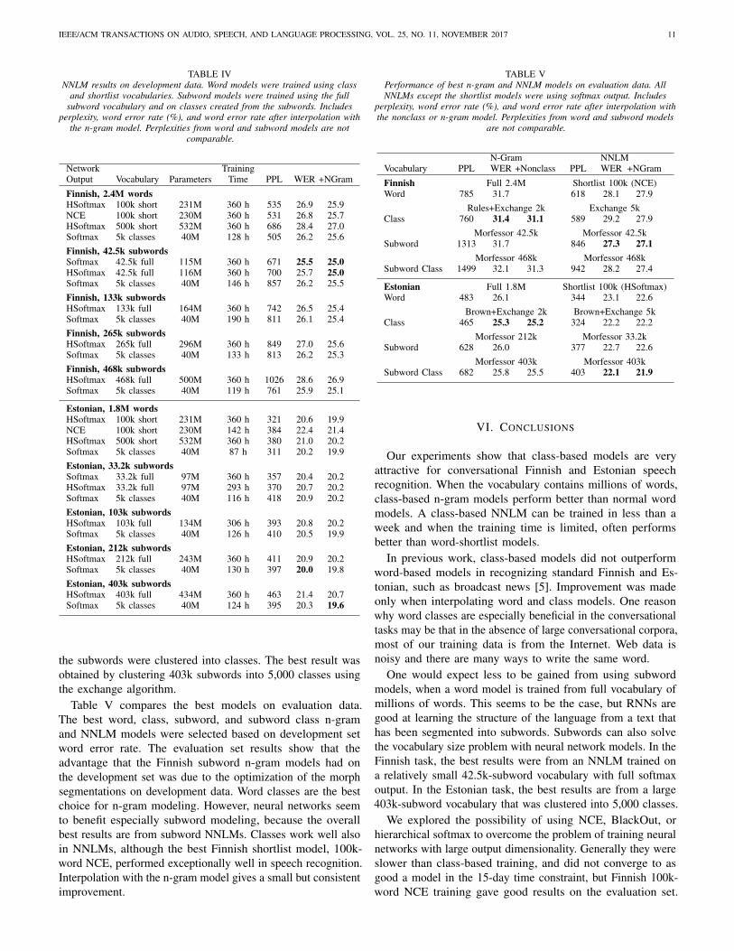
Table V compares the best models on evaluation data.The best word, class, subword, and subword class n-gramand NNLM models were selected based on development setword error rate. The evaluation set results show that theadvantage that the Finnish subword n-gram models had onthe development set was due to the optimization of the morphsegmentations on development data. Word classes are the bestchoice for n-gram modeling. However, neural networks seemto benefit especially subword modeling, because the overallbest results are from subword NNLMs. Classes work well alsoin NNLMs, although the best Finnish shortlist model, 100k-word NCE, performed exceptionally well in speech recognition.Interpolation with the n-gram model gives a small but consistentimprovement.

TABLE VPerformance of best n-gram and NNLM models on evaluation data. AllNNLMs except the shortlist models were using softmax output. Includes

perplexity, word error rate (%), and word error rate after interpolation withthe nonclass or n-gram model. Perplexities from word and subword models

are not comparable.

N-Gram NNLMVocabulary PPL WER +Nonclass PPL WER +NGram

Finnish Full 2.4M Shortlist 100k (NCE)Word 785 31.7 618 28.1 27.9

Rules+Exchange 2k Exchange 5kClass 760 31.4 31.1 589 29.2 27.9

Morfessor 42.5k Morfessor 42.5kSubword 1313 31.7 846 27.3 27.1

Morfessor 468k Morfessor 468kSubword Class 1499 32.1 31.3 942 28.2 27.4

Estonian Full 1.8M Shortlist 100k (HSoftmax)Word 483 26.1 344 23.1 22.6

Brown+Exchange 2k Brown+Exchange 5kClass 465 25.3 25.2 324 22.2 22.2

Morfessor 212k Morfessor 33.2kSubword 628 26.0 377 22.7 22.6

Morfessor 403k Morfessor 403kSubword Class 682 25.8 25.5 403 22.1 21.9

VI. CONCLUSIONS

Our experiments show that class-based models are veryattractive for conversational Finnish and Estonian speechrecognition. When the vocabulary contains millions of words,class-based n-gram models perform better than normal wordmodels. A class-based NNLM can be trained in less than aweek and when the training time is limited, often performsbetter than word-shortlist models.

In previous work, class-based models did not outperformword-based models in recognizing standard Finnish and Es-tonian, such as broadcast news [5]. Improvement was madeonly when interpolating word and class models. One reasonwhy word classes are especially beneficial in the conversationaltasks may be that in the absence of large conversational corpora,most of our training data is from the Internet. Web data isnoisy and there are many ways to write the same word.

One would expect less to be gained from using subwordmodels, when a word model is trained from full vocabulary ofmillions of words. This seems to be the case, but RNNs aregood at learning the structure of the language from a text thathas been segmented into subwords. Subwords can also solvethe vocabulary size problem with neural network models. In theFinnish task, the best results were from an NNLM trained ona relatively small 42.5k-subword vocabulary with full softmaxoutput. In the Estonian task, the best results are from a large403k-subword vocabulary that was clustered into 5,000 classes.

We explored the possibility of using NCE, BlackOut, orhierarchical softmax to overcome the problem of training neuralnetworks with large output dimensionality. Generally they wereslower than class-based training, and did not converge to asgood a model in the 15-day time constraint, but Finnish 100k-word NCE training gave good results on the evaluation set.


The mixed results could mean that some details have beenoverlooked in our implementation of sampling-based softmax.

In both tasks we obtained the best word error rates from asubword NNLM interpolated with a subword n-gram model.In the Finnish task the best result was 27.1 %, which is a 14.5% relative improvement from the 31.7 % WER given by ourbaseline 4-gram model. The best result in the Estonian task,21.9 %, is a 16.1 % relative improvement from our 26.1 %baseline WER. These are the best results achieved in thesetasks, and better than our previously best results by a largemargin. The best previously published results are 48.4 % WERin the Finnish task [11] and 52.7 % WER in the Estonian task[49].

The corpus weighting methods that we used in NNLMtraining showed potential for improvement, but more thoroughresearch should be done on how to select optimal weights.

VII. ACKNOWLEDGEMENTS

Computational resources were provided by the Aalto Science-IT project.

REFERENCES

[1] S. Enarvi and M. Kurimo, “Studies on training text selection for conver-sational finnish language modeling,” in Proc. International Workshop onSpoken Language Translation (IWSLT), Dec. 2013, pp. 256–263.

[2] T. Hirsimaki, M. Creutz, V. Siivola, M. Kurimo, S. Virpioja, andJ. Pylkkonen, “Unlimited vocabulary speech recognition with morphlanguage models applied to Finnish,” Computer Speech & Language,vol. 20, no. 4, pp. 515–541, Oct. 2006.

[3] V. Siivola, T. Hirsimaki, M. Creutz, and M. Kurimo, “Unlimitedvocabulary speech recognition based on morphs discovered in anunsupervised manner,” in Proc. EUROSPEECH. ISCA, Sep. 2003,pp. 2293–2296.

[4] M. Kurimo, A. Puurula, E. Arisoy, V. Siivola, T. Hirsimaki, J. Pylkkonen,T. Alumae, and M. Saraclar, “Unlimited vocabulary speech recognitionfor agglutinative languages,” in Proc. HLT-NAACL. Stroudsburg, PA,USA: Association for Computational Linguistics, Jun. 2006, pp. 487–494.

[5] M. Varjokallio, M. Kurimo, and S. Virpioja, “Class n-gram modelsfor very large vocabulary speech recognition of Finnish and Estonian,”in Proc. International Conference on Statistical Language and SpeechProcessing (SLSP), P. Kral and C. Martın-Vide, Eds. Cham, Switzerland:Springer International Publishing, Oct. 2016, pp. 133–144.

[6] R. Botros, K. Irie, M. Sundermeyer, and H. Ney, “On efficient training ofword classes and their application to recurrent neural network languagemodels,” in Proc. INTERSPEECH. ISCA, Sep. 2015, pp. 1443–1447.

[7] J. Dehdari, L. Tan, and J. van Genabith, “Scaling up word clustering,”in Proc. NAACL HLT Demonstrations Session, J. DeNero, M. Finlayson,and S. Reddy, Eds. Association for Computational Linguistics, Jun.2016, pp. 42–46.

[8] M. Song, Y. Zhao, and S. Wang, “Exploiting different word clusteringsfor class-based rnn language modeling in speech recognition,” in Proc.ICASSP. IEEE, Mar. 2017, pp. 5735–5739.

[9] W. Chen, D. Grangier, and M. Auli, “Strategies for training largevocabulary neural language models,” in Proc. ACL, Aug. 2016, pp.1975–1985.

[10] H. Schwenk and J.-L. Gauvain, “Training neural network language modelson very large corpora,” in Proc. HLT/EMNLP. Stroudsburg, PA, USA:Association for Computational Linguistics, Oct. 2005, pp. 201–208.

[11] S. Enarvi and M. Kurimo, “TheanoLM – an extensible toolkit for neuralnetwork language modeling,” in Proc. INTERSPEECH, Sep. 2016, pp.3052–3056.

[12] J. Goodman, “Classes for fast maximum entropy training,” in Proc.ICASSP, vol. 1. IEEE, May 2001, pp. 561–564.

[13] M. Gutmann and A. Hyvarinen, “Noise-contrastive estimation: A newestimation principle for unnormalized statistical models,” in Proc. Inter-national Conference on Artificial Intelligence and Statistics (AISTATS).New Jersey, USA: Society for Artificial Intelligence and Statistics, May2010, pp. 297–304.

[14] S. Ji, S. V. N. Vishwanathan, N. Satish, M. J. Anderson, andP. Dubey, “Blackout: Speeding up recurrent neural network languagemodels with very large vocabularies,” in Proc. International Conferenceon Learning Representations (ICLR), 2016. [Online]. Available:https://arxiv.org/abs/1511.06909

[15] P. F. Brown, P. V. deSouza, R. L. Mercer, V. J. D. Pietra, and J. C.Lai, “Class-based n-gram models of natural language,” ComputationalLinguistics, vol. 18, no. 4, pp. 467–479, Dec. 1992.

[16] R. Kneser and H. Ney, “Forming word classes by statistical clusteringfor statistical language modelling,” in Contributions to QuantitativeLinguistics, R. Kohler and B. B. Rieger, Eds. Dordrecht, the Netherlands:Kluwer Academic Publishers, 1993, pp. 221–226.

[17] S. Martin, J. Liermann, and H. Ney, “Algorithms for bigram and trigramword clustering,” in Proc. EUROSPEECH. ISCA, Sep. 1995, pp. 1253–1256.

[18] T. Mikolov, S. W. tau Yih, and G. Zweig, “Linguistic regularitiesin continuous space word representations,” in Proc. NAACL HLT.Stroudsburg, PA, USA: Association for Computational Linguistics, Jun.2013, pp. 746–751.

[19] T. Mikolov, K. Chen, G. Corrado, and J. Dean, “Efficient estimationof word representations in vector space,” in Proc. InternationalConference on Learning Representations (ICLR) Workshops, 2013.[Online]. Available: https://arxiv.org/abs/1301.3781

[20] R. Sproat, A. W. Black, S. Chen, S. Kumar, M. Ostendorf, andC. Richards, “Normalization of non-standard words,” Computer Speech& Language, vol. 15, no. 3, pp. 287–333, Jul. 2001.

[21] B. Han and T. Baldwin, “Lexical normalisation of short text messages:Makn sens a #twitter,” in Proc. ACL HLT. Stroudsburg, PA, USA:Association for Computational Linguistics, Jun. 2011, pp. 368–378.

[22] I. Listenmaa and F. M. Tyers, “Automatic conversion of colloquial Finnishto standard Finnish,” in Proc. Nordic Conference of ComputationalLinguistics (NODALIDA), B. Megyesi, Ed. Linkoping UniversityElectronic Press / ACL, May 2015, pp. 219–223.

[23] M. Creutz and K. Lagus, “Unsupervised discovery of morphemes,” inProc. ACL 2002 Workshop on Morphological and Phonological Learning(MPL), vol. 6. Stroudsburg, PA, USA: Association for ComputationalLinguistics, 2002, pp. 21–30.

[24] ——, “Unsupervised models for morpheme segmentation and morphologylearning,” ACM Transactions on Speech and Language Processing (TSLP),vol. 4, no. 1, pp. 3:1–3:34, Jan. 2007.

[25] M. Creutz, T. Hirsimaki, M. Kurimo, A. Puurula, J. Pylkkonen, V. Siivola,M. Varjokallio, E. Arisoy, M. Saraclar, and A. Stolcke, “Morph-basedspeech recognition and modeling of out-of-vocabulary words acrosslanguages,” ACM Transactions on Speech and Language Processing(TSLP), vol. 5, no. 1, pp. 3:1–3:29, Dec. 2007.

[26] O. Kohonen, S. Virpioja, and K. Lagus, “Semi-supervised learning ofconcatenative morphology,” in Proc. Meeting of the ACL Special InterestGroup on Computational Morphology and Phonology. Uppsala, Sweden:Association for Computational Linguistics, July 2010, pp. 78–86.

[27] S. Virpioja, P. Smit, S.-A. Gronroos, and M. Kurimo, “Morfessor2.0: Python implementation and extensions for Morfessor Baseline,”Department of Signal Processing and Acoustics, Aalto University,Report 25/2013 in Aalto University publication series SCIENCE +TECHNOLOGY, 2013.

[28] V. Siivola, T. Hirsimaki, and S. Virpioja, “On growing and pruningKneser-Ney smoothed n-gram models,” IEEE Transactions on Audio,Speech & Language Processing, vol. 15, no. 5, pp. 1617–1624, 2007.

[29] P. Smit, S. Virpioja, and M. Kurimo, “Improved subword modeling forWFST-based speech recognition,” in Proc. INTERSPEECH. ISCA, Aug.2017, pp. 2551–2555.

[30] T. Mikolov, M. Karafiat, L. Burget, J. Cernocky, and S. Khudanpur, “Re-current neural network based language model,” in Proc. INTERSPEECH.ISCA, Sep. 2010, pp. 1045–1048.

[31] S. Hochreiter and J. Schmidhuber, “Long short-term memory,” NeuralComputation, vol. 9, no. 8, pp. 1735–1780, Nov. 1997.

[32] R. K. Srivastava, K. Greff, and J. Schmidhuber, “Training very deepnetworks,” in Advances in Neural Information Processing Systems 28,C. Cortes, N. D. Lawrence, D. D. Lee, M. Sugiyama, and R. Garnett, Eds.Red Hook, NY, USA: Curran Associates, Inc., 2015, pp. 2377–2385.

[33] N. Srivastava, G. Hinton, A. Krizhevsky, I. Sutskever, and R. Salakhutdi-nov, “Dropout: A simple way to prevent neural networks from overfitting,”The Journal of Machine Learning Research, vol. 15, no. 1, pp. 1929–1958,Jun. 2014.

[34] J. Park, X. Liu, M. J. F. Gales, and P. C. Woodland, “Improvedneural network based language modelling and adaptation,” in Proc.INTERSPEECH. ISCA, Sep. 2010, pp. 1041–1044.


[35] T. N. Sainath, B. Kingsbury, V. Sindhwani, E. Arisoy, and B. Ramab-hadran, “Low-rank matrix factorization for deep neural network trainingwith high-dimensional output targets,” in Proc. ICASSP. IEEE, May2013, pp. 6655–6659.

[36] H.-K. Kuo, E. Arisoy, A. Emami, and P. Vozila, “Large scale hierarchicalneural network language models,” in Proc. INTERSPEECH. ISCA, Sep.2012, pp. 1672–1675.

[37] F. Morin and Y. Bengio, “Hierarchical probabilistic neural network lan-guage model,” in Proc. International Workshop on Artificial Intelligenceand Statistics (AISTATS), R. G. Cowell and Z. Ghahramani, Eds. NewJersey, USA: Society for Artificial Intelligence and Statistics, Jan. 2005,pp. 246–252.

[38] H. S. Le, I. Oparin, A. Messaoudi, A. Allauzen, J.-L. Gauvain, andF. Yvon, “Large vocabulary SOUL neural network language models,” inProc. INTERSPEECH. ISCA, Aug. 2011, pp. 1469–1472.

[39] E. Grave, A. Joulin, M. Cisse, D. Grangier, and H. Jegou, “Efficientsoftmax approximation for GPUs,” in Proc. ICML, D. Precup and Y. W.Teh, Eds., vol. 70. PMLR, Aug. 2017, pp. 1302–1310.

[40] Y. Bengio and J.-S. Senecal, “Quick training of probabilistic neural netsby importance sampling,” in Proc. International Workshop on ArtificialIntelligence and Statistics (AISTATS), C. M. Bishop and B. J. Frey, Eds.New Jersey, USA: Society for Artificial Intelligence and Statistics, Jan.2003.

[41] Y. Shi, W. Q. Zhang, M. Cai, and J. Liu, “Variance regularization ofRNNLM for speech recognition,” in Proc. ICASSP. IEEE, May 2014,pp. 4893–4897.

[42] A. Sethy, S. F. Chen, E. Arisoy, and B. Ramabhadran, “Unnormalizedexponential and neural network language models,” in Proc. ICASSP.IEEE, Apr. 2015, pp. 5416–5420.

[43] X. Chen, X. Liu, M. J. F. Gales, and P. C. Woodland, “Recurrent neuralnetwork language model training with noise contrastive estimation forspeech recognition,” in Proc. ICASSP. IEEE, Apr. 2015, pp. 5411–5415.

[44] T. Mikolov, S. Kombrink, L. Burget, J. Cernocky, and S. Khudanpur,“Extensions of recurrent neural network language model,” in Proc.ICASSP. IEEE, May 2011, pp. 5528–5531.

[45] A. Mnih and G. E. Hinton, “A scalable hierarchical distributed languagemodel,” in Advances in Neural Information Processing Systems 21,D. Koller, D. Schuurmans, Y. Bengio, and L. Bottou, Eds. Red Hook,NY, USA: Curran Associates, Inc., 2009, pp. 1081–1088.

[46] A. Mnih and Y. W. Teh, “A fast and simple algorithm for training neuralprobabilistic language models,” in Proc. ICML, J. Langford and J. Pineau,Eds. New York, NY, USA: Omnipress, Jul. 2012, pp. 1751–1758.

[47] T. Mikolov, I. Sutskever, K. Chen, G. Corrado, and J. Dean, “Distributedrepresentations of words and phrases and their compositionality,” inAdvances in Neural Information Processing Systems 26, C. J. C. Burges,L. Bottou, M. Welling, Z. Ghahramani, and K. Q. Weinberger, Eds. RedHook, NY, USA: Curran Associates, Inc., 2013, pp. 3111–3119.

[48] M. Sundermeyer, R. Schluter, and H. Ney, “Lattice decoding andrescoring with long-span neural network language models,” in Proc.INTERSPEECH. ISCA, Sep. 2014, pp. 661–665.

[49] M. Kurimo, S. Enarvi, O. Tilk, M. Varjokallio, A. Mansikkaniemi,and T. Alumae, “Modeling under-resourced languages for speechrecognition,” Language Resources and Evaluation (LRE), Feb. 2016.[Online]. Available: https://doi.org/10.1007/s10579-016-9336-9

[50] D. J. Iskra, B. Grosskopf, K. Marasek, H. van den Heuvel, F. Diehl,and A. Kießling, “SPEECON – speech databases for consumer devices:Database specification and validation,” in Proc. International Conferenceon Language Resources and Evaluation (LREC), May 2002, pp. 329–333.

[51] Aalto University, Department of Signal Processing and Acoustics, “AaltoUniversity DSP Course Conversation Corpus 2013–2017, DownloadableVersion,” 2017. [Online]. Available: http://urn.fi/urn:nbn:fi:lb-2017092133

[52] M. Lennes, “Segmental features in spontaneous and read-aloud Finnish,”in Phonetics of Russian and Finnish. General Introduction. Spontaneousand Read-Aloud Speech, V. de Silva and R. Ullakonoja, Eds. PeterLang GmbH, 2009, pp. 145–166.

[53] E. Meister, L. Meister, and R. Metsvahi, “New speech corpora at IoC,”in Proceedings of the XXVII Fonetiikan paivat – Phonetics Symposium,E. Meister, Ed. Tallinn, Estonia: TUT Press, Feb. 2012, pp. 30–33.

[54] A. Stolcke, “SRILM — an extensible language modeling toolkit,” inProc. ICSLP, Sep. 2002, pp. 901–904.

[55] J. Duchi, E. Hazan, and Y. Singer, “Adaptive subgradient methods foronline learning and stochastic optimization,” The Journal of MachineLearning Research, vol. 12, pp. 2121–2159, Jul. 2011.

[56] D. Povey, A. Ghoshal, G. Boulianne, L. Burget, O. Glembek, N. Goel,M. Hannemann, P. Motlicek, Y. Qian, P. Schwarz, J. Silovsky,G. Stemmer, and K. Vesely, “The Kaldi speech recognition toolkit,” inASRU Demonstration Session. IEEE Signal Processing Society, Dec.

2011. [Online]. Available: http://publications.idiap.ch/downloads/papers/2012/Povey ASRU2011 2011.pdf

[57] D. Povey, V. Peddinti, D. Galvez, P. Ghahremani, V. Manohar, X. Na,Y. Wang, and S. Khudanpur, “Purely sequence-trained neural networksfor ASR based on lattice-free MMI,” in Proc. INTERSPEECH, Sep. 2016,pp. 2751–2755.

[58] T. Ko, V. Peddinti, D. Povey, and S. Khudanpur, “Audio augmentation forspeech recognition,” in Proc. INTERSPEECH, Sep. 2015, pp. 3586–3589.

[59] C. Allauzen, M. Mohri, and B. Roark, “Generalized algorithms forconstructing statistical language models,” in Proc. Annual Meeting ofthe ACL. Sapporo, Japan: Association for Computational Linguistics,July 2003, pp. 40–47.

Seppo Enarvi received the Lic.Sc. in technologydegree in computer and information science fromAalto University, Espoo, Finland, in 2012. He pursuesto finish his Ph.D. on conversational Finnish speechrecognition during 2017. His research interests arein machine learning, currently focusing on languagemodeling using neural networks.

Peter Smit received the M.Sc. in technology degreein computer science from Aalto University, Espoo,Finland, in 2011. He is currently a doctoral student inthe Department of Signal Processing and Acousticsat Aalto University. His research interests are inmachine learning and speech recognition and hiscurrent focus is subword-modeling techniques andautomatic speech recognition for underresourcedlanguages.

Sami Virpioja received the D.Sc. in technologydegree in computer and information science fromAalto University, Espoo, Finland, in 2012. Between2013 and 2017 was a research scientist at LingsoftInc., Helsinki, Finland. Currently he is a senior datascientist at Utopia Analytics Oy, Helsinki, Finland,and a postdoctoral researcher in the Department ofSignal Processing and Acoustics at Aalto University.His research interests are in machine learning andnatural language processing.

Mikko Kurimo (SM’07) received the D.Sc. (Ph.D.)in technology degree in computer science from theHelsinki University of Technology, Espoo, Finland,in 1997. He is currently an associate professor in theDepartment of Signal Processing and Acoustics atAalto University, Finland. His research interests arein speech recognition, machine learning and naturallanguage processing.


ERRATUM

A highway network layer uses a separate bias for its gate,distinguished by the index σ in Equation 6. The index wasmissing in the published paper.

ieee/acm transactions on audio, speech, …senarvi.github.io/publications/taslp2017.pdf ·...

Documents