ieee transactions on medical imaging, vol. 30, · pdf fileieee transactions on medical...

IEEE TRANSACTIONS ON MEDICAL IMAGING, VOL. 30, NO. 9, SEPTEMBER 2011 1649

A Fast Wavelet-Based Reconstruction Methodfor Magnetic Resonance Imaging

M. Guerquin-Kern*, M. Häberlin, K. P. Pruessmann, and M. Unser

Abstract—In this work, we exploit the fact that wavelets canrepresent magnetic resonance images well, with relatively fewcoefficients. We use this property to improve magnetic resonanceimaging (MRI) reconstructions from undersampled data witharbitrary k-space trajectories. Reconstruction is posed as anoptimization problem that could be solved with the iterativeshrinkage/thresholding algorithm (ISTA) which, unfortunately,converges slowly. To make the approach more practical, wepropose a variant that combines recent improvements in convexoptimization and that can be tuned to a given specific k-spacetrajectory. We present a mathematical analysis that explains theperformance of the algorithms. Using simulated and in vivo data,we show that our nonlinear method is fast, as it accelerates ISTAby almost two orders of magnitude. We also show that it remainscompetitive with TV regularization in terms of image quality.

Index Terms—Compressed sensing, fast iterative shrinkage/thresholding algorithm (FISTA), fast weighted iterative shrinkage/thresholding algorithm (FWISTA), iterative shrinkage/thresh-olding algorithm (ISTA), magnetic resonance imaging (MRI),non-Cartesian, nonlinear reconstruction, sparsity, thresholdedLandweber, total variation, undersampled spiral, wavelets.

I. INTRODUCTION

M AGNETIC RESONANCE IMAGING scanners providedata that are samples of the spatial Fourier transform

(also know as k-space) of the object under investigation. TheShannon–Nyquist sampling theory in both spatial and k-spacedomains suggests that the sampling density should correspondto the field-of-view (FOV) and that the highest sampled fre-quency is related to the pixel width of the reconstructed images.However, constraints in the implementation of the k-space tra-jectory that controls the sampling pattern (e.g., acquisition du-ration, scheme, smoothness of gradients) may impose locallyreduced sampling densities. Insufficient sampling results in re-constructed images with increased noise and artifacts, particu-larly when applying gridding methods.

Manuscript received January 05, 2011; revised March 22, 2011; acceptedMarch 26, 2011. Date of publication April 07, 2011; date of current versionAugust 31, 2011. This work was supported by the Swiss National CompetenceCenter in Biomedical Imaging (NCCBI) and the Center for BiomedicalImaging of the Geneva-Lausanne Universities and EPFL. Asterisk indicatescorresponding author.

*M. Guerquin-Kern is with the Biomedical Imaging Group, École Polytech-nique Fédérale de Lausanne, CH-1015 Lausanne, Switzerland.

M. Unser is with the Biomedical Imaging Group, École PolytechniqueFédérale de Lausanne, CH-1015 Lausanne, Switzerland.

M. Häberlin and K. P. Pruessmann are with the Institute for Biomedical En-gineering, ETH Zürich, CH-8092 Zürich. Switzerland.

Color versions of one or more of the figures in this paper are available onlineat http://ieeexplore.ieee.org.

Digital Object Identifier 10.1109/TMI.2011.2140121

The common and generic approach to alleviate the recon-struction problem is to treat the task as an inverse problem [1]. Inthis framework, ill-posedness due to a reduced sampling densityis overcome by introducing proper regularization constraints.They assume and exploit additional knowledge about the ob-ject under investigation to robustify the reconstruction.

Earlier techniques used a quadratic regularization term,leading to solutions that exhibit a linear dependence upon themeasurements. Unfortunately, in the case of severe undersam-pling (i.e., locally low sampling density) and depending on thestrength of regularization, the reconstructed images still sufferfrom noise propagation, blurring, ringing, or aliasing errors. Itis well known in signal processing that the blurring of edgescan be reduced via the use of nonquadratic regularization. Inparticular, -wavelet regularization has been found to outper-form classical linear algorithms such as Wiener filtering in thedeconvolution task [2].

Indicative of this trend as well is the recent advent of Com-pressed Sensing (CS) techniques in MRI [3], [4]. These let usdraw two important conclusions.

• The introduction of randomness in the design of trajecto-ries favors the attenuation of residual aliasing artifacts be-cause they are spread incoherently over the entire image.

• Nonlinear reconstructions—more precisely, -regulariza-tion—outperform linear ones because they impose con-straints that are better matched to MRI images.

Many recent works in MRI have focused on nonlinear re-construction via total variation (TV) regularization, choosingfinite differences as a sparsifying transform [3], [5]–[7]. Non-quadratic wavelet regularization has also received some atten-tion [3], [8]–[11], but we are not aware of a study that comparesthe performance of TV against -wavelet regularization.

Various algorithms have been recently proposed for solvinggeneral linear inverse problems subject to -regularization.Some of them deal with an approximate reformulation ofthe regularization term. This approximation facilitates re-construction sacrificing some accuracy and introducing extradegrees of freedom that make the tuning task laborious. Instead,the iterative shrinkage/thresholding algorithm [2], [12], [13](ISTA) is an elegant and nonparametric method that is mathe-matically proven to converge. A potential difficulty that needsto be overcome is the slow convergence of the method whenthe forward model is poorly conditioned (e.g., low samplingdensity in MRI). This has prompted research in large-scaleconvex optimization on ways to accelerate ISTA. The efforts sofar have followed two main directions.

• Generic multistep methods that exploit the result of pastiterations to speed up convergence, among them: two-step

0278-0062/$26.00 © 2011 IEEE

1650 IEEE TRANSACTIONS ON MEDICAL IMAGING, VOL. 30, NO. 9, SEPTEMBER 2011

iterative shrinkage/thresholding [14] (TwIST), Nesterovschemes [15]–[17], fast ISTA [18] (FISTA), and mono-tonic FISTA [19] (MFISTA).

• Methods that optimize wavelet-subband-dependent param-eters with respect to the reconstruction problem: multilevelthresholded Landweber (MLTL) [20], [21] and subbandadaptive ISTA (SISTA) [22].

In this work, we exploit the possibility of combining and tai-loring the two generic types of accelerating strategies to comeup with a new algorithm that can speedup the convergence of thereconstruction and that can accomodate for every given k-spacetrajectory. Here, we first consider single-coil reconstructionsthat do not use sensitivity knowledge. In a second time, we con-firm the results with SENSE reconstructions [1].

We propose a practical reconstruction method that turns outto sensibly outperform linear reconstruction methods in termsof reconstruction quality, without incurring the protracted re-construction times associated with nonlinear methods. This isa crucial step in the practical development of nonlinear algo-rithms for undersampled MRI, as the problem of fixing the reg-ularization parameter is still open. We also provide a mathemat-ical analysis that justifies our algorithm and facilitates the tuningof the underlying parameters.

This paper is structured as follows. In Section II, we describethe basic data-formation model for MRI and derive the dis-crete forward model. The representation of the object by waveletbases is considered in Section II-C2; in particular, we legitimatethe use of a wavelet regularization term (which promotes spar-sity) to distinguish the solution from other possible candidates.In Section III, we propose a fast algorithm for solving the non-linear reconstruction problem and present theoretical argumentsto explain its superior speed of convergence. Finally, we presentin Section IV an experimental protocol to validate and compareour practical method with existing ones. We focus mainly onreconstruction time and signal-to-error ratio (SER) with respectto the reference image.

II. MRI AS AN INVERSE PROBLEM

In this section, we present the MR acquisition model and therepresentation of the signal that is used to specify the reconstruc-tion problem. The main acronyms and notations are summarizedin Table 1. We motivate the sparsity assumptions in the waveletdomain and the variational approach with regularization thatis used to solve the inverse problem of imaging.

A. Model of Data Formation

1) Physics: We consider MRI in two dimensions, in whichcase a 2D plane is excited. The time-varying magnetic gradientfields that are imposed define a trajectory in the (spatial) Fourierdomain that is often referred to as k-space. We denote by thecoordinates in that domain. The excited spins, which behave asradio-frequency emitters, have their precessing frequency andphase modified depending on their positions. The modulatedpart of the signal received by a homogeneous coil is given by

(1)

It corresponds to the Fourier transform of the spin density thatwe refer to as object. The measurements, concatenated in thevector , correspond to sampled values ofthis Fourier transform at the frequency locations along thek-space trajectory.

2) Model for the Original Data:a) Spatial discretization of the object: From here on, we

consider that the Fourier domain and, in particular, the samplingpoints , are scaled to make the Nyquist sampling intervalunity. This can be done without any loss of generality if thespace domain is scaled accordingly. Therefore, we model theobject as a linear combination of pixel-domain basis functions

that are shifted replicates of some generating function , sothat

(2)

with

(3)

In MRI, the implicit choice for is often Dirac’s delta.Different discretizations have been proposed, for exampleby Sutton et al. [23] with as a boxcar function or later byDelattre et al. [24] with B-splines. But it has not been workedout in detail how to get back the image for general that arenoninterpolating, which is the case, for instance for B-splinesof order greater than 1. The image to be reconstructed [i.e., thesampled version of the object ] is obtained by filtering thecoefficients with the discrete filter

(4)

where denotes the Fourier transform of .b) Wavelet discretization: In the wavelet formalism, some

constraints apply on . It must be a scaling function that sat-isfies the properties for a multiresolution [25]. In that case, thewavelets can be defined as linear combinations of the andthe object is equivalently characterized by its coefficients inthe orthonormal wavelet basis. We refer to Mallat’s book [26]for a full review on wavelets. There exists a discrete wavelettransform (DWT) that bijectively maps the coefficients to thewavelet coefficients that represent the same object in a con-tinuous wavelet basis. In the rest of the paper, we represent thisDWT by the synthesis matrix . Note that the matrix multi-plications and have efficient filterbankimplementations.

B. Matrix Representation of the Model

Since a FOV determines a finite number of coefficients, we handle them as a vector , keeping the discrete coordi-

nates as implicit indexing. By simulating the imaging of theobject (2), and by evaluating (1) for , we find that thenoise-free measurements are given by

(5)

GUERQUIN-KERN et al.: A FAST WAVELET-BASED RECONSTRUCTION METHOD FOR MAGNETIC RESONANCE IMAGING 1651

where , the MRI system matrix, is decomposed as

(6)

There, is a space-domain vector such that .A more realistic data-formation model is

(7)

or(8)

with and a residual vector representing the effect onmeasurements of noise and scanner imprecisions. The inverseproblem of MRI is then to recover the coefficients (or )from the corrupted measurements . Its degree of difficultydepends on the magnitude of the noise and the conditioning ofthe matrix (or ).

C. Variational Formulation

1) General Framework: The solution is defined as theminimizer of a cost function that involves two terms: the datafidelity and the regularization that penalizes unde-sirable solutions. This is summarized as

(9)

where the regularization parameter balances the twoconstraints. In MRI, is usually assumed to be a realization ofa white Gaussian process, which justifies the choice

as a proper log-likelihood term. The ill-conditioning in-herent to undersampled trajectories imposes the use of the suit-able regularization term .

Standard Tikhonov regularization corresponds to thequadratic term and leads to the closed-form

linear solution that istractable both theoretically and numerically. When the recon-struction problem is sufficiently overdetermined to make noisepropagation negligible, regularization is dispensable and theleast-squares solution, which corresponds to Tikhonov with

, is adequate. The approach is statistically optimal if theobject can also be considered as a realization of a Gaussianprocess. Unfortunately, this assumption is hardly justified fortypical MR images. The quality of the solution obtained by thismeans quickly breaks down when undersampling increases.

TV reconstruction is related to the sum of the Euclideannorms of the gradient of the object. In practice, it is defined as

, where the operator returns pixelwise the-norm of finite differences. The use of TV regularization is

particularly appropriate for piecewise-constant objects such asthe Shepp–Logan (SL) phantom.

2) Sparsity-Promoting Regularization: The main idea in thiswork is to exploit the fact that the object can be well repre-sented by few nonzero coefficients (sparse representation) in anorthonormal basis of functions . Formally, we write that

• , (sparse support)and

• (small error).It is well documented that typical MRI images admit sparse

representation in bases such as wavelets or block DCT [3].

The -norm is a good measure of sparsity with interestingmathematical properties (e.g., convexity). Thus, among the can-didates that are consistent with the measurements, we favor a so-lution whose wavelet coefficients have a small -norm. Specif-ically, the solution is formulated as

(10)

with

(11)

This is the general solution for wavelet-regularized inverseproblems considered by [13] as well as many other authors.

III. WAVELET REGULARIZATION ALGORITHMS

In this section, we present reconstruction algorithms thathandle constraints expressed in the wavelet domain whilesolving the minimization problem (10). By introducingweighted norms instead of simple Lipschitz constants, we re-visit the principle of the standard ISTA algorithm and simplifythe derivation and analysis of this class of algorithms. We endup with a novel algorithm that combines different accelerationstrategies and we provide a convergence analysis. Finally, wepropose an adaptation of the fast algorithm to implement therandom-shifting technique that is commonly used to improveresults in image restoration.

A. Weighted Norms

Let us first define the weighted norm corresponding to a pos-itive-definite symmetric weight matrix as .The requirement that the eigenvalues of —denoted

—must be positive leads to the norm property

B. Principle of ISTA Revisited

An important observation to understand ISTA is to see thatthe nonlinear shrinkage operation, sometimes called soft-thresh-olding, solves a minimization problem [27], with

(12)

By separability of norms, this applies component-wise to vec-tors of . Thismeans that the -regularized denoising problem (i.e., whenin (11) is the identity matrix) is precisely solved by a shrinkageoperation.

The iterative shrinkage/thresholding algorithm (ISTA) [2],[13], also known as thresholded Landweber (TL), generates asequence of estimates that converges to the minimizerof (11) when it is unique. The idea is to define at each step anew functional whose minimizer will be thenext estimate

(13)


Two constraints must be considered for the definition of .

1) It is sufficient for the convergence of the algorithm thatis an upper bound of and matches it at

; this guarantees that the sequence ismonotonically decreasing.

2) The inner minimization (13) should be performed by asimple shrinkage operation to ensure the rapidity andaccuracy of the algorithm.

In accordance with Constraint (1), can take the genericquadratically augmented form

(14)

with the constraint that is positive definite, wherethe weighting matrix plays the role of a tuning parameter.

Then, ISTA corresponds to the trivial choice ,with the value of chosen to be greater or equal to theLipschitz constant of the gradient of , so that

.Let us define , , and

(15)

Then, using standard linear algebra, we can write(16)

(17)

This shows that Constraint (2) is automatically satisfied.Note that both the intermediate variable in (15) and the

threshold values will vary depending on .

Algorithm 1: ISTA

Repeat ;

Beck and Teboulle [18, Thm. 3.1] showed that this algorithmdecreases the cost function in direct proportion to the numberof iterations , so that . Here, wepresent a slightly extended version of their original result whichis valid for any reference point during iterations.

Proposition 1: Let be the sequence generated by Al-gorithm 1 with . Then, for any ,

(18)

Proof: [18, Thm. 3.1] gives the result for . Con-sider a sequence such that . As the iterationdoes not depend on , we get . The result fol-lows immediately.

Selecting as small as possible will clearly favor the speed ofconvergence. It also raises the importance of a “warm” startingpoint.

Among the variants of ISTA, FISTA, proposed by Beck andTeboulle [18], ensures state-of-the-art convergence propertieswhile preserving a comparable computational cost. Thanks toa controlled over-relaxation at each step, FISTA quadraticallydecreases the cost function, with .

C. Subband Adaptive ISTA (SISTA)

SISTA is an extension of the ISTA that was introduced byBayram and Selesnick [22]. Here, we propose an interpretationof SISTA as a particular case of (14) with a weighting matrixthat replaces advantageously the step size in (15). The ideais to use a diagonal weighting matrix —if it isnot diagonal, Constraint (2) would not be fulfilled—with coef-ficients that are constant within a wavelet subband.

1) SISTA: In the same fashion as for ISTA, (15) and (17) canbe adapted to subband-dependent steps and thresholds.Accord-ingly, SISTA is described in Algorithm 2.

Algorithm 2: SISTA

Repeat ;

2) Convergence Analysis: By considering the weightedscalar product instead of , we can adapt theconvergence proof of ISTA by Beck and Teboulle (see Propo-sition 1). This result is new, to the best of our knowledge.

Proposition 2: Let be the sequence generated by Al-gorithm 2 with . Then, for any ,

(19)

Proof: We rewrite the cost function (11) with the change ofvariable . We then apply ISTA to solve that problemwith , , and (Note that

is positive-definite if is positive-definite). Theiteration can be rewritten,in terms of the original variable, as

. The latter is an iteration of SISTA (see Algorithm 2).According to Proposition 1, we have

, which translates directly into theproposed result.

Therefore, by comparing Propositions 1 and 2, an improvedconvergence is expected. The main point is that, for a “warm”starting point or after few iterations , the weightednorm in (19) can yield significantly smaller values than the oneweighted by in (18).

3) Selection of Weights: Bayram and Selesnick [22] providea method to select the values of for SISTA. To presentthis result, let us introduce some notations. We denote by

an index that scans all the wavelet subbands, coarsescale included, by the corresponding weight constant,and by the corresponding block of . We also define

. The authors of [22]show that, for each subband, the condition

(20)

is sufficient to impose the positive definiteness ofthat is required in (14). In the present context, we propose tocompute the values by using the power iteration method,once for a given wavelet family and k-space sampling strategy.


Fig. 1. Reference images from left to right: in vivo brain, SL reference, and wrist.

D. Best of Two Worlds: Fast Weighted ISTA (FWISTA)

Taking advantage of the ideas developed previously, we de-rive an algorithm that corresponds to the subband adaptive ver-sion of FISTA. In the light of the minimization problem (11),FWISTA generalizes the FISTA algorithm using a parametricweighted norm. We give its detailed description in Algorithm3, where the modifications with respect to FISTA is the SISTAstep in the loop.

Algorithm 3: FWISTA

input: , , , and ;

Initialization: , , ;

repeat

(SISTA step);

;

;

;

until desired tolerance is reached;

return ;

In the same fashion as for SISTA, we revisit the convergenceresults of FISTA [18, Thm. 4.4] for FWISTA.

Proposition 3: Let be the sequence generated by Al-gorithm 3. Then, for any

(21)

Proof: In the spirit of the proof of Proposition 2, weconsider the change of variable and applyFISTA to solve the new reconstruction problem. The step

is equivalent to. The convergence results of FISTA

[18, Thm. 4.4] applies on the sequence , which leads to.

This result shows the clear advantage of FWISTA comparedto ISTA (Proposition 1) and SISTA (Proposition 2). Moreover,we note that FWISTA can be simply adapted in order to imposea monotonic decrease of the cost functional value, in the samefashion as MFISTA. The same convergence properties apply[19, Thm. 5.1].

E. Random Shifting

Wavelet bases perform well the compression of signals butcan introduce artifacts that can be attributed to their relativelack of shift-invariance. In the case of regularization, this can beavoided by switching to a redundant dictionary. The downside,however, is a significant increase in computational cost. Alter-natively, the practical technique referred to as random shifting(RS) [2] can be used. Applying random shifting is much simplerand computationally more efficient than considering redundanttransforms and leads to sensibly improved reconstruction.

Here, we propose a variational interpretation that motivatesour implementation of FWISTA with RS (see Algorithm 4). Weconsider the DWT , with , where

represent the different shifting operations required to get atranslation-invariant DWT. The desired reconstruction would bedefined as the minimizer of

(22)

In 1D, this formulation includes TV regularization, inother words a single-level undecimated Haar WT withoutcoarse-scale thresholding.

Rewriting (22) in terms of wavelet coefficients, we get

(23)

with

(24)


For a current estimate, we select a transform and performa step in the minimization of the cost with respect to whilekeeping , for fixed. A SISTA step is used, as the mini-mization subproblem (24) takes the form (11). The minimizersof the functionals are expected to correspond to images closeto each other and to the minimizer of (22). In the first iterationsof the algorithm, the minimization steps with respect to anyare functionally equivalent (i.e., the modification is mostly ex-plained by the gradient step). This motivates the use of FWISTAiterations at first and the switch to ISTA steps afterwards.

As the scheme is intrinsically greedy, we do not have a theo-retical guarantee of convergence. Yet, in practice, we have ob-served that the SER stabilizes at a much higher value than it doeswhen using ISTA schemes with no RS (cf Fig. 4).

Algorithm 4: FWISTA with RS

input: , , , , ;

Consider the sequence of DWT with RS: ;

Initialization: , , , , ,;

repeat

;

;

(cost-function evaluation);

if then

;

if then

;

;

;

;

;

;

until stopping condition is met;

IV. EXPERIMENTS

A. Implementation Details

Our implementation uses Matlab 7.9 (Mathworks, Natick,MA). The reconstructions run on a 64-bit 8-core computer,clock rate 2.8 GHz, 8 GB RAM (DDR2 at 800 MHz), MacOS X 10.6.5. For all iterative algorithms, a key point is thatmatrices are not stored in memory. They only represent op-erations that are performed on vectors (images). In particular,

is computed once per dataset. Matrix-to-vectormultiplication with , specifically, , have anefficient implementation thanks to the convolution structure ofthe problem [28], [29]. For these Fourier precomputations, we

Fig. 2. Time evolution of the SER with respect to the minimizer for severalISTA algorithms. Times to reach 35 dB are delineated.

Fig. 3. Time evolution of the difference in cost function value with respect tothe minimizer for several ISTA algorithms.

used the NUFFT algorithm [30] that is made available online.For wavelet transforms, we used the code provided online[21]. This Fourier-domain implementation proved to be fasterthan Matlab’s when considering reconstructed images smallerthan 256 256 and the Haar wavelet. It must also be noted thatthe 2D-DFT were performed using the FFTW library whichefficiently parallelizes computations.

For Tikhonov regularizations, we implemented the classicalconjugate gradient (CG) algorithm, with the identity as the reg-ularization matrix. For TV regularizations, we considered the it-eratively reweighted least-squares algorithm (IRLS), which cor-responds to the additive form of half-quadratic minimization[31], [32]. We used 15 iterations of CG to solve the linear innerproblems, always starting from the current estimate, which iscrucial for efficiency. For the weights that permit the quadraticapproximation of the TV term, we stabilized the inversion ofvery small values.

We implemented ISTA, SISTA, and FWISTA as described inSection III, with the additional possibility to use random shifting(see Section IV-C2). For the considered reconstructions usingour method, described in Algorithm 4, was a reason-able choice. The Haar wavelet transform was used, with threedecomposition levels when no other values are mentioned. As is

1http://www.eecs.umich.edu/~fessler/code/2http://bigwww.epfl.ch/algorithms/mltldeconvolution


TABLE IGLOSSARY

usual for wavelet-based reconstructions, the regularization wasnot applied to the coarse-level coefficients.

Reconstructions were limited to the pixels of the ROI for allalgorithms. The regularization parameter was systematicallyadjusted such that the reconstruction mean-squared error (MSE)inside the ROI was minimal. For practical situations where theground-truth reference is not available, it is possible to adjustby considering well-established techniques such as the discrep-ancy principle, generalized cross validation, or L-curve method[33].

B. Spiral MRI Reconstruction

In this section, we focused on the problem of reconstructingimages of objects weighted by the receiving channel sensitivity,given undersampled measurements. This problem, which in-volves single-channel data and hence differs from SENSE, ischallenging for classical linear reconstructions as it generates

Fig. 4. Time evolution of the SER for several algorithms for the SL simulationusing Haar wavelets.

artifacts and propagates noise. We considered spiral trajectorieswith 50 interleaves, with an interleave sampling density reducedby a factor compared to Nyquist for the highest fre-quencies and an oversampling factor 3.5 along the trajectory.Spiral acquisition schemes are attractive because of their ver-satility and the fact that they can be implemented with smoothgradient switching [34], [35].

We validate the results with the three sets of data that wepresent below. The corresponding reference images are shownin Fig. 1.

1) MR Scanner Acquisitions: The data were collected on a3T Achieva system (Philips Medical Systems, Best, The Nether-lands). A field camera with 12 probes was used to monitor theactual k-space trajectory [36]. An array of eight head coils pro-vided the measurements. We acquired in vivo brain data from ahealthy volunteer with parameters ms and

ms. The excitation slice thickness was 3 mm with a flip angleof 30 . The trajectory was designed for a FOV of 25 cm with apixel size 1.5 mm. It was composed of 100 spiral interleaves.The interleaf distance for the highest sampled frequencies de-fined a fraction of the Nyquist sampling density .

The subset used for reconstruction corresponds to half of the100 interleaves. The corresponding reduction factor, defined asthe ratio of the distance of neighboring interleaves with theNyquist distance, is .

2) Analytical Simulation: We used analytical simulations ofthe SL brain phantom with a similar coil sensitivity, followingthe method described in [37]. The values of these simulated datawere scaled to have the same mean spatial value (i.e., the samecentral k-space peak) as the brain reference image. A realizationof complex Gaussian noise was added to this synthetic k-spacedata, with a variance corresponding to 40 dB SNR. The 176

176 rasterization of the analytical object provided a reliablereference for comparisons.

3) Simulation of a Textured Object: A second simulationwas considered with an object that is more realistic than theSL phantom. We chose a 512 512 MR image of a wristthat showed little noise and interesting textures. We simulatedacquisitions with the same coil profile and spiral trajectory(176 176 reconstruction matrix), in presence of a 40 dB SNR


TABLE IIVALUES OF THE OPTIMAL SER AND CORRESPONDING REGULARIZATION PARAMETERS ARE SHOWN FOR THE DIFFERENT WAVELET BASES

TABLE IIIRESULTS OF THE PROPOSED WAVELET METHOD FOR DIFFERENT WAVELET DECOMPOSITION DEPTHS. VALUES OF THE REGULARIZATIONPARAMETER, THE FINAL SER, THE RELATIVE MAXIMAL SPATIAL DOMAIN ERROR, AND THE TIME TO REACH 0.5 dB OF THE FINAL SER

TABLE IVRESULTS OF THE ALGORITHMS CG (LINEAR), IRLS (TV), AND OUR METHOD (WAVELETS) FOR DIFFERENT DEPTHS. VALUES OF THE REGULARIZATION

PARAMETER, THE FINAL SER, THE RELATIVE MAXIMAL SPATIAL DOMAIN ERROR, AND THE TIME TO REACH 0.5 dB OF THE FINAL SER

Fig. 5. Result of different reconstruction algorithms for the three experiments. For each reconstruction, the performance in SER with respect to the reference(top-left), the reconstruction time (top-right), and the number of iterations (bottom-right) are shown.

Gaussian complex noise. The height of the central peak wasalso adjusted to correspond to that of the brain data. The refer-ence image was obtained by sinc-interpolation, by extractingthe lowest frequencies in the DFT.

C. Results

In this section, we present the different experiments we con-ducted. The two main reconstruction performance measures thatwe considered are as follows.


• Reconstruction duration, which excludes all aforemen-tioned precomputations and the superfluous monitoringoperations.

• Signal to error ratio with respect to a reference, de-fined as and

. Practically,the references are either the ground-truth images or theminimizer of the cost functional. It is known that SER isnot a foolproof measure of visual improvement but largeSER values are encouraging and generally correlate withgood image quality.

1) Convergence Performance of IST-Algorithms: In this firstexperiment, we compared the convergence properties of the dif-ferent ISTA-type algorithms, as presented in Section III, withthe Haar wavelet transform. The data we considered are thoseof the MR wrist image. The regularization parameter was ad-justed to maximize the reconstruction SER with respect to theground-truth data. The actual minimizer of the cost functional,which is the common fixed-point of this family of algorithms,was estimated by iterating FWISTA 100 000 times.

The convergence results are shown in Figs. 2 and 3 for thesimulation of the MR wrist image. Similar graphs are obtainedusing the other sets of data.

For a fixed number of iterations, FISTA schemes (FISTAand FWISTA) require roughly 10% additional time comparedto ISTA and SISTA. In spite of this fact, their asymptoticsuperiority appears clearly in both figures. The slope of thedecrease of the cost functional in the log-log plot of Fig. 3reflects the convergence properties in Propositions 1, 2, and3. When considering the first iterations, which are of greatestpractical interest, the algorithms with optimized parameters(SISTA and FWISTA) perform better than ISTA and FISTA(see Fig. 3). The times required by each algorithm to reacha 30 dB SER (considered as a threshold value to perceivedchanges) are 415 s (ISTA), 53 s (SISTA), 12.7 s (FISTA), and4.4 s (FWISTA). With respect to this criterion, SISTA presentsan eight-fold speedup over ISTA, while FWISTA presents a12-fold speedup over SISTA and nearly a three-fold speedupover FISTA. It follows that FWISTA is practically close to twoorders of magnitude faster than ISTA.

2) Choice of the Wavelet Transform and Use of RandomShifting: The algorithms presented in Section III apply for anyorthogonal wavelet basis. For the considered application, wewant to study the influence of the basis on performance. In thisexperiment we considered the Battle–Lemarié spline wavelets[26] with increasing degrees, taking into account the necessarypostfilter mentioned in (4).

We compared the best results for several bases. They wereobtained with FWISTA after practical convergence and are re-ported in Table II. Fig. 4 illustrates the time evolution of the SERusing ISTA and FWISTA in the case of the SL reconstruction.Similar graphs are obtained with the other experiments.

It is known that the Haar wavelet basis efficiently approxi-mates piecewise-constant objects like the SL phantom, whichis consistent with our results. On the other hand, splines ofhigher degree, which have additional vanishing moments, per-form better on the textured images (upper part of Table II).

Fig. 6. Evolution of the performance of the algorithms. From top to bottom: SLsimulation, wrist simulation, and brain data. Times required to reach 0.5 dBof the asymptotic value are indicated.

We present in the lower part of Table II the performancesobserved when using ISTA with RS. We conclude that, in thecase of realistic data, it is crucial to use RS as it improvesresults by at least 0.7 dB, whatever the wavelet basis is. Theremarkable aspect there is that the Haar wavelet transformwith RS consistently performs best. Two important things canbe seen in Fig. 4: FWISTA is particularly efficient duringthe very first iterations, while SISTA with RS yields the bestasymptotic results in terms of SER and stability. Our methodcombines both advantages.

In Table III, we present the results obtained using differentdepths of the wavelet decompositions. Our reconstructionmethod is used together with the Haar wavelet transform andRS. The performances are similar but there seems to be an ad-vantage in using several decomposition levels both in terms of


Fig. 7. Reconstructions and error maps of different IST-algorithms with RS for the wrist experiment. For each reconstruction, the performance in SER with respectto the reference (top-left), the reconstruction time (top-right), and the number of iterations (bottom-right) are shown.

SER and reconstruction speed. The FWISTA scheme seems torecoup the cost of the wavelet transform operations associatedto an increase in the depth of decomposition.

3) Practical Performance: We report in Table IV the re-sults obtained for different reconstruction experiments usingstate-of-the-art linear reconstruction, TV regularization, and ourmethod. The images obtained when running the different algo-rithms after approximately 5 s, and after practical convergenceas well, are shown in Fig. 5. We display in Fig. 6 the time evolu-tion of the SER for the different experiments. In each case, weemphasize the time required to reach 0.5 dB of the asymptoticvalue of SER. Finally, we present in Fig. 7 the reconstructionand error maps of the different IST-algorithms at different mo-ments of reconstruction. This was done with the wrist simulatedexperiment using the Haar wavelet basis and RS.

Firstly, we observe that TV and our method achieve similarSER (Table IV) and image quality (Fig. 5). They both clearlyoutperform linear reconstruction, with a SER improvementfrom 1.5 to 3 dB, depending on the degree of texture in the orig-inal data. Moreover, the pointwise maximal reconstruction errorappears to always be smaller with nonlinear reconstructions.Due to the challenging reconstruction task, which significantlyundersamples of the k-space, residual artifacts remain in thelinear reconstructions and at early stages of the nonlinear ones.Although the k-space trajectory is exacly the same in the threecases, artifacts are less perceived in the in vivo reconstructions,while they stand out for the synthetic experiments.

Secondly, it clearly appears that the linear reconstruction,implemented with CG, leads to the fastest convergence, un-fortunately with suboptimal quality. For a reconstruction timeone order of magnitude longer, our accelerated method providesbetter reconstructions. This is illustrated in Fig. 5 for reconstruc-tion times of the order of five seconds (columns 1, 2, and 4).

Finally, we observe in Fig. 7 the superiority of the proposedFWISTA over the other types of algorithms. For the given re-construction times, it consistently exhibits better image qualityas can be seen in both reconstructions and error maps.

D. SENSE MRI Reconstruction

Our reconstruction method is applicable to linear MRimaging modalities. In this section, we report results obtainedon a SENSE reconstruction problem. The data were acquiredwith the same scanner setup as in Section IV-B1. This time,the data from the eight receiving channels were used for recon-struction, as well as an estimation of the sensitivity maps. Anin vivo gradient echo EPI sequence of a brain was performedwith T2 contrast. The data was acquired with the followingparameters: excitation slice thickness of 4 mm, ms,

ms, flip angle of 80 , and trajectory composed of13 interleaves, supporting a 200 200 reconstruction matrixwith pixel resolution 1.18 mm 1.18 mm. The oversamplingratio along the readout direction was 1.62.

The reference image was obtained using the complete set ofdata and performing an unregularized CG-SENSE reconstruc-


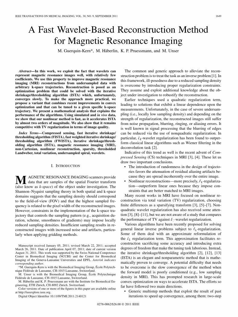
Fig. 8. Reconstructions (left column) and error maps (right column) for theSENSE EPI experiment using CG (first row), IRLS-TV (second row), and ourmethod (third row). For each reconstruction, the performance in SER withrespect to the reference (top-left corner), the reconstruction time (top-rightcorner), the number of iterations (bottom-right corner), and a magnification ofthe central part (bottom-left) are shown.

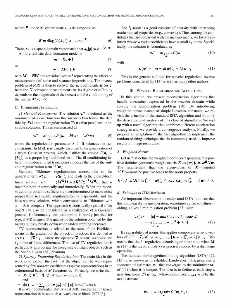
Fig. 9. Evolution of the performance of the algorithms. Times required to reach0.5 dB of the asymptotic value are indicated.

tion. The reconstruction involved 3 of the 13 interleaves, repre-senting a significant undersampling ratio .

The images obtained using regularized linear reconstruction(CG), TV (IRLS), and our method are presented in Fig. 8. InFig. 9, the SER evolution with respect to time is shown forthe three methods. The times to reach 0.5 dB of the asymp-totic SER value are 5.9 s (CG), 49.1 s (IRLS), and 22.8 s (ourmethod).

With this high undersampling, the errors maps show that re-constructions suffer from noise propagation mostly in the centerof the image. It appears that TV and our method improve quali-tatively and quantitatively image quality over linear reconstruc-tion (cf. Fig. 8). As it was observed in Section IV-B with thespiral MRI reconstructions, this in vivo SENSE experiment con-firms that our method is competitive with TV. In terms of recon-struction duration, our method proves to converge in a time thatis of the same order of magnitude as CG (cf. Fig. 9).

V. CONCLUSION

We proposed an accelerated algorithm for nonlinear wavelet-regularized reconstruction that is based on two complementaryacceleration strategies: use of adaptive subband thresholds plusmultistep update rule. We provided theoretical evidence that thisalgorithm leads to faster convergence than when using the ac-celerating techniques independently. In the context of MRI, theproposed strategy can accelerate the reference algorithm up totwo orders of magnitude. Moreover, we demonstrated that, byusing the Haar wavelet transform with random shifting, we areable to boost the performance of wavelet methods to make themcompetitive with TV regularization. Using different simulationsand in vivo data, we compared the practical performance of ourreconstruction method with other linear and nonlinear ones.

The proposed method is proved to be competitive with TVregularization in terms of image quality. It typically convergeswithin five seconds for the single channel problems considered.This brings nonlinear reconstruction forward to an order of mag-nitude of the time required by the state-of-the-art linear recon-structions, while providing much better quality.

ACKNOWLEDGMENT

The authors would like to thank J. Fessler and C. Vonesch tomake their implementations of NUFFT and multidimensionalwavelet transform available. We acknowledge C. Vonesch,I. Bayram, and D. Van De Ville for fruitful discussions. The au-thors would also like to thank P. Thévenaz for useful commentsand careful proofreading.

REFERENCES

[1] K. P. Pruessmann, M. Weiger, M. B. Scheidegger, and P. Boesiger,“SENSE: Sensitivity encoding for fast MRI,” Magn. Reson. Med., vol.42, no. 5, pp. 952–962, 1999.

[2] M. A. T. Figueiredo and R. D. Nowak, “An EM algorithm for wavelet-based image restoration,” IEEE Trans. Signal Process., vol. 12, no. 8,pp. 906–916, Aug. 2003.

[3] M. Lustig, D. L. Donoho, and J. M. Pauly, “Sparse MRI: The appli-cation of compressed sensing for rapid MR imaging,” Magn. Reson.Med., vol. 58, pp. 1182–1195, 2007.

[4] U. Gamper, P. Boesiger, and S. Kozerke, “Compressed sensing in dy-namic MRI,” Magn. Reson. Med., vol. 59, no. 2, pp. 365–373, 2008.

[5] K. T. Block, M. Uecker, and J. Frahm, “Undersampled radial MRIwith multiple coils. Iterative image reconstruction using a total vari-ation constraint,” Magn. Reson. Med., vol. 57, no. 6, pp. 1086–1098,2007.

[6] L. Ying, L. Bo, M. C. Steckner, W. Gaohong, W. Min, and L. Shi-Jiang,“A statistical approach to SENSE regularization with arbitrary k-spacetrajectories,” Magn. Reson. Med., vol. 60, pp. 414–421, 2008.

[7] B. Liu, K. King, M. Steckner, J. Xie, J. Sheng, and L. Ying, “Reg-ularized sensitivity encoding (SENSE) reconstruction using Bregmaniterations,” Magn. Reson. Med., vol. 61, no. 1, pp. 145–152, 2009.

[8] M. Lustig, J. H. Lee, D. L. Donoho, and J. M. Pauly, “Faster imagingwith randomly perturbed, undersampled spirals and reconstruc-tion,” in Proc. ISMRM, 2005.


[9] B. Liu, E. Abdelsalam, J. Sheng, and L. Ying, “Improved spiral sensereconstruction using a multiscale wavelet model,” in Proc. ISBI, 2008,pp. 1505–1508.

[10] L. Chaâri, J.-C. Pesquet, A. Bebazza-Benyahia, and P. Ciuciu, “Auto-calibrated regularized parallel MRI reconstruction in the wavelet do-main,” in Proc. ISBI, 2008, pp. 756–759.

[11] M. Guerquin-Kern, D. Van De Ville, C. Vonesch, J.-C. Baritaux, K.P. Pruessmann, and M. Unser, “Wavelet-regularized reconstruction forrapid MRI,” in Proc. ISBI, 2009, pp. 193–196.

[12] . : J. Bect, L. Blanc-Féraud, G. Aubert, and A. Chambolle, “A -uni-fied variational framework for image restoration,” Lecture Notes inComputer Science, vol. 3024, pp. 1–13, 2004.

[13] I. Daubechies, M. Defrise, and C. De Mol, “An iterative thresholdingalgorithm for linear inverse problems with a sparsity constraint,”Commun. Pure Appl. Math., vol. 57, no. 11, pp. 1413–1457, 2004.

[14] J. M. Bioucas-Dias and M. A. T. Figueiredo, “A new twist: Two-step it-erative shrinkage/thresholding algorithms for image restoration,” IEEETrans. Image Process., vol. 16, no. 12, pp. 2992–3004, Dec. 2007.

[15] Y. E. Nestorov, Gradient methods for minimizing composite objectivefunction CORE Rep., Tech. Rep., 2007.

[16] P. Weiss, “Algorithmes rapides d’optimisation convexe. Application àla restoration d’images et à la détection de changements,” Ph.D. disser-tation, Univ. Nice, Nice, France, Dec. 2008.

[17] S. Becker, J. Bobin, and E. J. Candès, NESTA: A fast and accurate first-order method for sparserecovery California Inst. Technol., Pasadena,2009, Tech. Rep..

[18] A. Beck and M. Teboulle, “A fast iterative shrinkage-thresholding al-gorithm for linear inverse problems,” SIAM J. Imag. Sci., vol. 2, no. 1,pp. 183–202, 2009.

[19] A. Beck and M. Teboulle, “Fast gradient-based algorithms for con-strained total variation image denoising and deblurring problems,”IEEE Trans. Image Process., vol. 18, no. 11, pp. 2419–2434, Nov.2009.

[20] C. Vonesch and M. Unser, “A fast thresholded Landweber algorithmfor wavelet-regularized multidimensional deconvolution,” IEEE Trans.Image Process., vol. 17, no. 4, pp. 539–549, Apr. 2008.

[21] C. Vonesch and M. Unser, “A fast multilevel algorithm for wavelet-regularized image restoration,” IEEE Trans. Image Process., vol. 18,no. 3, pp. 509–523, Mar., 2009.

[22] I. Bayram and I. W. Selesnick, “A subband adaptive iterative shrinkage/thresholding algorithm,” IEEE Trans. Signal Process., vol. 58, no. 3,pp. 1131–1143, Mar. 2010.

[23] B. P. Sutton, D. C. Noll, and J. A. Fessler, “Fast, iterative image re-construction for MRI in the presence of field inhomogeneities,” IEEETrans. Med. Imag., vol. 22, no. 2, pp. 178–188, Feb. 2003.

[24] B. Delattre, J.-N. Hyacinthe, J.-P. Vallée, and D. Van De Ville, “Spline-based variational reconstruction of variable density spiral k-space datawith automatic parameter adjustment,” in Proc. ISMRM, 2009, p. 2066.

[25] M. Unser and T. Blu, “Wavelet theory demystified,” IEEE Trans. SignalProcess., vol. 51, no. 2, pp. 470–483, 2003.

[26] S. Mallat, A Wavelet Tour of Signal Processing. New York: Aca-demic, 1999.

[27] A. Chambolle, R. A. DeVore, N.-Y. Lee, and B. J. Lucier, “Non-linear wavelet image processing: Variational problems, compression,and noise removal through wavelet shrinkage,” IEEE Trans. SignalProcess., vol. 7, no. 3, pp. 319–335, Mar. 1998.

[28] F. T. W. A. Wajer and K. P. Pruessmann, “Major speedup of recon-struction for sensitivity encoding with arbitrary trajectories,” in Proc.ISMRM, 2001, p. 625.

[29] J. A. Fessler, S. Lee, V. T. Olafsson, H. R. Shi, and D. C. Noll,“Toeplitz-based iterative image reconstruction for MRI with correc-tion for magnetic field inhomogeneity,” IEEE Trans. Signal Process.,vol. 53, no. 9, pp. 3393–3402, Sep. 2005.

[30] J. A. Fessler and B. P. Sutton, “Nonuniform fast Fourier transformsusing min-max interpolation,” IEEE Trans. Signal Process., vol. 51,no. 2, pp. 560–574, 2003.

[31] D. Geman and C. Yang, “Nonlinear image recovery with half-quadraticregularization,” IEEE Trans. Image Process., vol. 4, no. 7, pp. 932–946,Jul. 1995.

[32] F. Champagnat and J. Idier, “A connection between half-quadratic cri-teria and EM algorithms,” IEEE Signal Process. Lett., vol. 11, no. 9,pp. 709–712, Sep. 2004.

[33] W. C. Karl, “Regularization in image restoration and reconstruction,”in Handbook of Image and Video Processing, A. C. Bovik, Ed. NewYork: Elsevier, 2005, pp. 183–202.

[34] G. H. Glover, “Simple analytic spiral k-space algorithm,” Magn. Reson.Med., vol. 42, no. 2, pp. 412–415, 1999.

[35] D.-H. Kim, E. Adalsteinsson, and D. M. Spielman, “Simple analyticvariable density spiral design,” Magn. Reson. Med., vol. 50, no. 1, pp.214–219, 2003.

[36] C. Barmet, N. De Zanche, B. J. Wilm, and K. P. Pruessmann, “Atransmit/receive system for magnetic field monitoring of in vivo MRI,”Magn. Reson. Med., vol. 62, no. 1, pp. 269–276, 2009.

[37] M. Guerquin-Kern, F. I. Karahanoglu, D. Van De Ville, K. P. Pruess-mann, and M. Unser, “Analytical form of Shepp-Logan phantom forparallel MRI,” in Proc. ISBI, 2010, pp. 261–264.

ieee transactions on medical imaging, vol. 30, · pdf fileieee transactions on medical...

Documents