boundary detection by constrained optimization - · pdf fileieee transactions on pattern ......

IEEE TRANSACTIONS ON PATTERN ANALYSIS AND MACHINE INTELLIGENCE. VOL. 12. NO. 7, JULY 1990 609

Boundary Detection by Constrained Optimization ‘ DONALD GEMAN, MEMBER, IEEE, STUART GEMAN, MEMBER, IEEE, CHRISTINE GRAFFIGNE, AND

PING DONG, MEMBER, IEEE

Abstract-We use a statistical framework for finding boundaries and for partitioning scenes into homogeneous regions. The model is a joint probability distribution for the a r ray of pixel gray levels and an a r ray of “labels.” In boundary finding, the labels a re binary, zero, or one, representing the absence o r presence of boundary elements. In partitioning, the label values a r e generic: two labels a re the same when the corresponding scene locations a r e considered to belong to the same region. The distribution incorporates a measure of disparity between certain spatial features of pairs of blocks of pixel gray levels, using the Kolmogorov-Smirnov nonparametric measure of difference between the distributions of these features. Large disparities encourage intervening boundaries and distinct partition labels. The number of model parameters is minimized by forbidding label configurations that a r e inconsistent with prior beliefs, such as those defining very small regions, o r redundant or blindly ending boundary placements. Forbidden configurations a re assigned probability zero. We examine the MAP (mar- imum a posterion’) estimator of boundary placements and partitionings. The forbidden states introduce constraints into the calculation of these configurations. Stochastic relaxation methods a re extended to accommodate constrained optimization, and experiments are performed on some texture collages and some natural scenes.

i Zndex Terms-Annealing, Bayesian inference, boundary finding, constrained optimization, Gibbs distribution, MAP estimate, Markov random field, segmentation, stochastic relaxation, texture discrimination.

I . INTRODUCTION ANY problems in image analysis, from signal res- M toration to object recognition, involve representa-

tions of the observed data, usually radiant energy or range measurements, in terms of unobserved attributes or label variables. These representations may be conclusive, or serve as intermediate data structures for further analysis, perhaps involving additional data, assorted “sketches,” or stored models. This work concems two such represen-

Manuscript received April 18, 1988; revised September 14, 1989. Rec- ommended for acceptance by A. K. Jain. The work of D. Geman and P. Dong was supported in part by the Office of Naval Research under Contract “14-86-K-0027. The work of S . Geman and C . Graffigne was supported in part by the Army Research Office under Contract DAAL03-86- K-0171 to the Center for Intelligent Control Systems, by the National Sci- ence Foundation under Grant DMS-8352087, and by the General Motors Research Laboratories.

D. Geman is with the Department of Mathematics and Statistics, Uni- versity of Massachusetts, Amherst, MA 01003.

S . Geman is with the Division of Applied Mathematics, Brown Univer- sity, Providence, RI 02912.

C . Graffigne was with the Division of Applied Mathematics, Brown University, Providence, RI 02912. She is now with the French National Center for Scientific Research (CNRS), Equipe de Statistique Appliquke, Bitiment 425, UniversitC de Paris-Sud, 91405 Orsay Cedex, France.

P. Dong was with the Department of Mathematics and Statistics, Uni- versity of Massachusetts, Amherst, MA 01003. He is now with Codex, Mansfield. MA 02048.

’

!

,

,

IEEE Log Number 90361 12.

tations related to image segmentation: partition and boundary labels. These, in tum, are special cases of a general “label model” in the form of an “energy functional’’ involving two components, one of which ex- presses the interactions between the labels and the (intensity) data, and the other encodes constraints derived from general information or expectations about label patterns. The labeling we seek is, by definition, the minimum of this energy.

The partition labels do not classify. Instead they are generic and are assigned to blocks of pixels; the size of the blocks (or label resolution) is variable, and depends on the resolution of the data and the intended interpreta- tions. The boundary labels are just “on”/“off ,” and are also of variable resolution, associated with an interpixel sublattice. In both cases, the interaction term incorporates a measure of disparity between certain spatial features of pairs of blocks of pixel gray levels, using the Kolmogo- rov-Smirnov nonparametric measure of difference between the distributions of these features. Large disparities encourage intervening boundaries and distinct partition labels. The number of model parameters is reduced by forbidding label configurations that are inconsistent with prior expectations, such as those defining very small regions, or redundant or blindly ending boundary placements. These forbidden states introduce constraints into the calculation of the optimal label configuration.

Both models are applied mainly to the problem of texture segmentation. The data is a gray-level image consisting of textured regions, such as a mosaic of microtextures from the Brodatz album [6], a patch of rug inside plastic, or radar-imaged ice floes in water. It is well- known that humans perceive “textural” boundaries between regions of approximately the same average brightness because the regions themselves, although containing sharp intensity changes, are perceived as “homogeneous” based on other properties, namely those involving the spatial distribution of intensity values. The goal, then, is to find the (visually) distinct texture regions, either by assigning categorical labels to the pixels, or by construct- ing a boundary map. Obviously, the problem is more difficult than texture classification, in which we are presented with only one texture from a given list; segmentation may be complicated by an absence of information about the number of textures, or about the size, shape, or number of regions.

There is no “model” for the individual textures, and hence no capacity for texture synthesis. Our approach is

0162-8828/90/0700-0609$01 .OO 0 1990 IEEE

610 IEEE TRANSACTIONS ON PATTERN ANALYSIS A N D MACHINE INTELLIGENCE. VOL. 12. NO. 7. JULY 1990

therefore different from those for classification and segmentation in which textures are discriminated based on model parameters which are estimated from specific texture samples. Partitionings and boundary placements are driven by the observed spatial statistics as summarized by selected features. Still, the labeling is not unsupervised because in some cases we use “training samples” to determine feature thresholds for the disparity measures; see Sections I1 and 111.

Since many visually distinct textures have nearly identical histograms, segmentation must rely on features, or transformations, which go beyond the raw gray levels, involving various spatial statistics. We experimented with several conventional classes of features, in particular the well-known ones based on cooccurrence matrices [ 161, [3 13, but finally adopted a new class based mainly on “directional residuals” and involving third and higher order distributions. However, our viewpoint is exactly that ex- pressed by Zobrist and Thompson [62], Triendl and Hen- dersen [59], and others: instead of trying to find exactly the “right” features to convert texture to tone differences, one should find a mechanism for integrating multiple, even redundant, ‘‘cues.’’ The label model provides a co- herent method for integrating such information and, simultaneously, organizing the label patterns.

Whereas texture discrimination may be regarded as the detection of discontinuities in surface composition, we also apply the boundary model to the problem of locating sudden changes in depth (occluding boundaries) or shape (surface creases, etc.). The idea is to define contours which are faithful to the 3-D scene but avoid the “non- physical” edges due to noise, digitization, texture, lighting, etc. In particular, the boundaries should be connected, unique, and reasonably smooth, unlike the typical output of a pure edge detector. Indeed, we formulate boundary detection as a single optimization problem, fus- ing the detection of edges with their pruning, linking, smoothing, and so on. Obviously, there are discontinuities, such as shadows, which are essentially impossible to distinguish from the occluding and shape boundaries, at least without information from multiple sensors or a rich knowledge base, in which case boundary classification becomes possible.

Our model enjoys some invariance properties. In particular, due to the use of the Kolmogorov-Smirnov distance, the detected labels are unaffected by linear changes in illumination, and in some cases by all monotone data transformations. Such distortions often result from sensor nonlinearities, digitizers, and film properties. In regard to rotation invariance, the estimated labeling will be independent of the relative orientation of the training samples with the image data to the extent that the features are rotation invariant. The pixel lattice precludes true invariance. However, since our collection of features is basically isotropic, our results are approximately invariant. See [38] for an approach to rotation-invariant classijica- tion.

Apparently, some of these ideas have been around for a while. For example, the Kolmogorov-Smirnov statistic is recommended in [51], and reference is made to still earlier papers; more recently, see [60]. Moreover, the dis- tributional properties of residuals (from surface-fitting) are advocated in [29], [48] for detecting discontinuities. It is certainly our contention that the statistical warehouse is full of useful tools for computer vision.

Finally, our model may be interpreted in a Bayesian framework as a “prior” joint probability distribution for the array of pixel gray levels and the array of labels. For- bidden configurations are assigned probability zero, and the label estimate is then associated with the MAP (maximum a posteriori) estimate. We shall discuss this interpretation in more detail later on. Suffice to say that, whereas our formulation of the problem and definition of the “best” labeling are formally independent of the stochastic outlook, our optimization procedures are in fact strongly motivated by this viewpoint. In fact, in order to deal with the more difficult textures, the deterministic (‘ ‘zero-temperature”) relaxation algorithm we use for most of our experiments must be replaced by a version of stochastic relaxation extended to accommodate constrained sampling and optimization.

A. Applications Texture is a dominant feature in remotely sensed im-

ages and regions cannot be distinguished by methods based solely on shading, such as edge detectors or clus- tering algorithms. Specifically, for example, one might wish to determine the concentration of ice in synthetic aperture radar images of the ocean, or analyze multispec- tral satellite data for land use classification. Another ap- plication is to wafer inspection: low magnification views of memory arrays appear as highly structured textures, and other geometries have a characteristic, but random, graining. In addition, the use of boundary maps as the input to further processing is ubiquitous in computer vision; for example, algorithms for stereopsis, optical flow, and simple object recognition are often based on matching boundary segments. Other applications include the analysis of medical images, automated navigation, and the detection of roads, faults, field boundaries, etc. in remotely sensed images. (Obviously no generic algorithm provides “off-the-shelf” solutions to real problems; genuine applications require substantial adaptations.)

B. Label Model Let x = { xs, s E S } and y = { yij, 1 5 i , j I N ]

denote, respectively, the labels and the data; thus x, is the label at “site” s E S and yQ is the gray-level at pixel ( i , j ) . The set S of label sites is a regular lattice, distinct from that of the pixels, and typically more sparse; the coarseness depends on the label resolution o. For partitioning, we associate each site s E S with a block of pixels, “sitting below it,” if we were to stack the label lattice on top of the pixel lattice. In the boundary model,

GEMAN et al. : BOUNDARY DETECTION BY CONSTRAINED OPTIMIZATION 61 1

Y; =

. pairs of nearby sites in S define boundary segments, and these are associated with pairs of pixel blocks, sitting “across from each other,” with respect to the segments

4 (see Fig. 6). Later, we will define a neighborhood system for S such that the bonding is nearest-neighbor (relative to a ) in the boundary model, whereas in the region model there are interactions at all scales. This has important con- sequences for the distribution of local minima in the “energy landscape”; see Section 11. Other energy functionals with global interactions can be found in [22], [26], and [471.

The “interaction” between x and y is defined in terms of an enerw function

Y, -

“ 4

The summation extends over all “neighboring pairs” (or “bonds”) ( s, t ), s, t E S ; 9,,t( y) is a measure of the disparity between the two blocks of pixel data associated with the label sites s, t E S . *,,,(x) depends only on the labels x, and x,. In fact, we simply take *,,,(x) = 1 - x,x, in the boundary model and *,,,(x) = SXs=,, in the partition model. In this way, in the “low energy states,” large disparities (a > 0) will typically be coupled with an active boundary (x, = x, = 1 ) or with dissimilar region labels (x, # x,) and small disparities (9 < 0) will be coupled with an inactive boundary (x, = 0 or x, = 0) or with equal region labels (x, = x,).

The interaction between the labels and the data is based on various disparity measures for comparing two (possibly distant) blocks of image data. These measures derive from the raw data as well as from various transformations. We experiment with several transformations y -+

y ’ for texture analysis, for example transformations of the form

where Eai = 1 and { tj } are pixels nearby to pixel t in the same row, column, or diagonal. We call these “directional residuals,” regarding Eaj y,, as a “predictor” of y,. We have also investigated raw gray levels ( y ‘ = y) , other features based on local measures of gray-level range, and isotropic versions of ( 1 . 1 ) . In any case, disparity is measured by the Kolmogorov-Smirnov statistic (or distance), a common tool in nonparametric statistics which has desirable invariance properties. (In particular, using the directional residuals, the disparity measure is invariant to linear distortions ( y o -, ayi/ + b ) of the raw data, and using the raw data itself for comparisons, the disparity measure is invariant to all monotone (data) transformations.) The general form of the 9 term is then

where 4 is monotone increasing, p denotes a distance based on the Kolmogorov-Smirnov statistic (see Section

11), and yif;, yiij) are the data in the two blocks associated with ( s, t ) for the ith transform. Often, we simply take m = 1 a n d y ( ” = y.

The other component in the model is a penalty function V(x) which counts the number of “taboo patterns” in x; states x for which V ( x ) > 0 are “forbidden.” For example, boundary maps are penalized for dead-ends, “clutter,” density, etc. whereas partitions are penalized for too many transitions or regions which are “too small. ”

Given the observed image y, our estimate i? = a ( y ) is then any solution to the constrained optimization problem

minimize,: v ( x ) = U ( x , y) . (1 .2) We seek to minimize the energy of the data-label interaction over all possible nonforbidden label states x.

The rationale for constrained optimization is that our expectations about certain types of labels are quite precise and rigid. For example, most “physical boundaries” are smooth, persistent, and well-localized; consequently it is reasonable to impose these assumptions on image boundaries, and corresponding restrictions on partition geometries. Contrast this with other inference problems, for example restoring an image degraded by blur and noise. Aside from contraints derived from scene-specific knowledge, the only reasonable generic constraints might be ‘‘piecewise continuity, ” and generally the degree of am- biguity favors more flexible constraints, such as those in U , or in the energy functions used in [20] and [22].

There are no multiplicative parameters in the model, such as the “smoothing” or “weighting” parameters in [3], [17], [19], [20], and [22]; in effect, the energy is U + X V with X = 00. Thresholds must be selected for the disparity measures; this may be done “in the blind,” but the performance of the algorithm is certainly increased if these choices are data-driven, either from prior experi- ence with the types of textures, or by extracting training samples, as we have done here (see Section V). Fortu- nately, the algorithm is not unduly sensitive to these choices within a certain range of values. Other inputs include the label resolution, block sizes, and penalty patterns. The algorithm is robust against these choices provided that modest information is available about the pixel resolution. The selection of penalty patterns is nearly self- evident: as already noted, our expectations about the ge- ometry of regions and boundaries are very concrete and easily encoded in local constraints.

C. Constrained Stochastic Relaxation The search for i , the optimal labeling, is based on a

version of stochastic relaxation which incorporates hard constraints. The theoretical foundations are laid out in [ 181, although there is enough information provided here (see Section IV) to keep this paper self-contained. (See also Grenander [28] and Linsker [41] for similar modifi- cations of stochastic relaxation.) We employ two algorithms, both of which are approximations to precise computational procedures, in which convergence is at least

__

612 IEEE TRANSACTIONS ON PATTERN ANALYSIS AND MACHINE INTELLIGENCE. VOL. 12. NO. 7, JULY 1990

theoretically guaranteed, if not always realized in practice.

Introduce a control parameter t corresponding to “temperature” and another control parameter X, corresponding to a Lagrange multiplier for the constraint V = 0. Let

where y (the data) is fixed, tk L 0, and X k 7 03. One

Monte Carlo sampling from the Gibbs measures with energy functions U,. If tk is fixed, then under suitable conditions on the growth of X k , the sequence xk converges to a sample from the Gibbs distribution with energy U , but restricted to V = 0, i.e., constrained to assign probability zero to the forbidden configurations. We refer to this as “constrained stochastic relaxation. ” On the other hand, if X k 7 03 and tk L 0, both at suitably (coupled) rates (see Section IV), then the sequence converges to a solution of (1.2); this is “constrained simulated annealing. ”

The first algorithm we use is deterministic, with the temperature fixed at zero, and is essentially the ICM (“iterated conditional mode”) algorithm of Besag [2], although X = hk 7 a. The convergence is rapid and the performance is sufficient for all but the most difficult images. The second algorithm is constrained stochastic relaxation with the temperature fixed at some “small” value (but, again, X = hk 7 03); the idea is simply that the very likely states of the constrained Gibbs distribution should be “close” to the mode, i.e., f. This “low temperature sampling’ ’ is more computationally demanding than ICM, but invariably arrives at a better labeling; see Section V on experiments.

D. Related Work The subject of edge detection is very active; however,

as we have already mentioned, the raw output of standard edge detectors, for example those based on differential operators, would generally require considerable “processing” to produce unique, smooth, persistent boundaries. The work in “regularization theory” [44], [49], as well as our earlier paper [20], is different in that “edge” or “line” process is employed there as a device for sus- pending continuity constraints in the context of recon- structing an image from sparse data, restoring an image corrupted by blur and noise, and similar tasks not aimed at boundary detection per se.

In contrast, there is much related work in the area of texture segmentation. In Triendl [58] and Triendl and Thompson [59], local property values referred to as “texture parameters” are computed in a neighborhood of each pixel and edge maps are computed for several principal components of these feature images. These maps are in- tegrated across components, and then spatially, resulting in a final boundary map. Similarly, in Thompson [57] (see also Zobrist and Thompson [62]), the idea is to integrate multiple cues into a single “distance function” which is a linear combination of elementary measures, and which

generates a sequence of states fk , k = 1 , 2, * - - 3 by

is intended to measure the overall similarity between two regions. Edges are then detected using the Robert’s cross gradient applied to this distance; there is no effort to or- ganize the responses. Our experiments compare favorably to those in [57] and [59], both of which utilize collages of natural textures similar to ours. Local filtering is also the focus of Laws’ approach [40], although the mechanism for combining cues is entirely different from ours.

Among the statistical approaches to texture segmentation are those in which the image data is regarded as a realization of a two-dimensional stochastic process, or random field. In Simchony and Chellappa [53] and in Derin and Cole [12], the image is modeled as a two-layered Markov random field: the “upper level” is the region process, a simple Ising-type process, and the “bottom level” is the observed intensity process, with some distribution (e.g., Gaussian) conditional on the regions. Both papers employ stochastic relaxation to search for the MAP and related estimators. Modestino et a l . [45] use random tessellations for the upper level and maximum likelihood estimation based on cooccurrence data for the labeling. In each case, the random field parameters are assumed known in advance or are estimated from training samples. The image data in [12] is generated from the model, and simpler than the actual texture collages in [53] and [45]. Again, our results compare favorably.

Finally, Kashyap and Eom [37] employ a “long correlation” random field model and statistical hypothesis testing to obtain a boundary map. Boundary placements are estimated in each small strip of the image based on least-squares estimates of the model parameters. There is no training data and the results are good, although, nat- urally, the boundaries are somewhat disorganized.

E. Stochastic Formulation This work is an extension, incorporating hard con-

straints, of a Bayesian paradigm in which prior probability models are constructed for both the observed and unobserved scene attributes. The degradation process is modeled as a conditional probability distribution, and the estimates are obtained by a form of Monte Carlo sampling. This framework has been applied by numerous re- searchers, including applications to image restoration [20], [2], [9], [24], [28], image synthesis [28], computed tomography [22], texture and boundary analysis [ 171, [53], [ 191 , [2 11 , [25], scene segmentation based on optical flow [47] or shading and texture [ 111, [ 131, frame-to- frame matching for computing optical flow and stereo disparity [36], and surface reconstruction [43], [44].

To facilitate placing our model in the general framework, let us write x = ( x L , x p ) , where x L is the vector of boundary or region labels, and x p is the vector of pixel gray levels. These are the relevant image attributes for the problem at hand. The prior distribution ll is a probability for x: 0 I n(x) I 1 , C , I I ( x ) = 1 , where C, is the summation over all configurations of x (all assignments of gray levels and boundary placements, for example). Adopting the Gibbs representation in the unconstrained

GEMAN et a / . : BOUNDARY DETECTION BY CONSTRAINED OPTIMIZATION

case we would represent II as

1 I

n(x ) = - exp { - i = C e x p { - X

The real-valued function U is called the energy, and evidently determines II. In our case we separate the prior energy into a pixel-label interaction term and a pure label contribution. The former, U ( x L , x p ), promotes placements of boundaries, or assignments of distinct labels, between regions in the image that demonstrate distinct spatial patterns. The pure label contribution is to inhibit “blind” endings of boundaries, redundant boundary representations, excessively small or thin regions, and other unexpected label configurations. Rather than inhibiting these configurations with high energy via large parameters, we have found it convenient, especially when work- ing with boundaries and partitionings, to extend this framework, by allowing ‘‘infinite energies” (zero probabilities) in the prior distribution. (See Moussouris [46] for an analysis of Gibbs measures with “forbidden states. ”) We forbid these configurations by introducing V = V ( x L ) 2 0 and concentrating on { x : V ( x L ) = O } . The prior, then, is of the form

The constraint, V ( x L ) = 0, amounts to a placement of infinite energy barriers in the “energy landscape. ” These inhibit the free flow that is essential to the good performance of stochastic relaxation; indeed the theory will1 in general break down, and convergence is no longer guaranteed. As indicated above, a simple and effective solution is to introduce the barriers gradually during the relaxation process. Again, the supporting convergence theory is spelled out in [ 181.

There is usually a problem-specific degradation that precludes directly observing x. It may be the blur and noise introduced by the camera and recording devices, the attenuated Radon transform that figures into emission tomography, or, as in this case, an “occlusion”: we assume the gray levels x p are observed (uncorrupted) whereas the labels x L are of course unobserved. Thus the data is y = x p and our only interest is in estimating the unobserved label process xL. II ( y I x ) is singular, and the posterior distribution for x L given the data is

There is skepticism about the MAP estimator: see, e.g., [2], [15], [44]. It has sometimes been found to be too “global,” leading to gross mislabeling in certain classification problems and “over-smoothing” in surface reconstruction and image restoration. (See [7] for a different view.) The discussion paper of Besag [2] has shed much light on the subject; see especially the remarks of Silver- man [52] on MAP versus simulations from the posterior n(x I y) , and the remarkable comparisons between the

__

613

exact MAP estimate and approximations derived from simulated annealing in the commentary of Greig, Por- teous, and Seheult [27]. However, pixel-based error measures are too local for boundary analysis. In particular, the Bayes rule based on misclassification error rate, namely the marginal (individual component) modes of n(x I y ) , is unsuitable because this estimator lacks the fine structure we expect of boundary maps; placement deci- sions cannot be based on the data alone-pending labels (i.e., context) must be considered. See [44], [50], and [61] for discussions of alternative loss functions and performance criteria.

11. PARTITION MODEL A . Partitionings

Denote the pixel (image) lattice { ( i , j ): 1 I i, j I N } by SI and let S, (formally S in Section I) be the label lattice, just a copy of SI in the case of the partition model. For each experiment, a resolution o is chosen, which determines a sublattice Sfp’ C s,, and the coarseness of the partitioning. Larger 0’s will correspond to coarser partitionings and give more reliable results (see Section V), but they lose boundary detail. Specifically, let

Recall that the observation process, or data, consists of gray levels y,, s E SI. With the usual gray-level discreti- zation, the state, or configuration, space for the data is

a,= { { y s } : s ~ S r , 0 _ ( y , ~ 2 5 5 )

The configuration space for the partitioning x is deter- mined by U and by a maximum number of allowed regions P :

a y ’ = { { x , ] : s E sp, 0 5 x, I P - 1 ) .

Recall that the labels are generic: x defines a partitioning by identifying sites with a given label (0 , 1, * . , p - 1) as belonging to the same region. Only the sublattice Sfp) is labeled, and a maximum number of labels (regions) is fixed a priori. A prior estimate of the number of distinct (but not necessarily connected) regions must be available, since the model often subdivides homogeneous regions when P is too large (see Section V). The boundary model (Section 111) is more robust in this regard.

Each label site s E S, is associated with a square block D, E SI of pixel sites centered at s. (Recall that S, is just a copy of S,; we sometimes use “s” ambiguously to reference a site in S, und the corresponding site in s/.) x, labels the pixels in 0,: { { yr }: r E D, } . As we will see shortly, the partitioning is based on the spatial statistics of these (overlapping) subimages. The size of D, is therefore important. We have experimented only with textures (the boundary model has been applied more generally), and is obvious that for these the pixel blocks { D, ) seSy must be large enough to capture the characteristic pattern of the texture, at least in comparison to the other textures

614 IEEE TRANSACTIONS ON PATTERN ANALYSlS AND MACHINE INTELLIGENCE, VOL. 12, NO. 7. JULY 1990

present. Of course, “large enough” is with respect to the features used, but in the absence of a multiscale analysis, an a priori choice of scale is unavoidable. In all of our experiments, 1 D, 1 = 441, a 21 x 21 square block of pixels. There is again a resolution issue: larger blocks char- acterize the textures more reliably, having less within-region variation, but boundary detail is sacrificed.

B. Label-Data Interaction We establish a neighborhood system on the label lattice

Sp’: each s E Sp’ is associated with a set of neighbors N , C Sp’. The system is symmetric, meaning that s E N , e r E N , . As we shall see, the neighborhood system largely determines the computational burden. For now we will proceed as though the neighborhood system is given, but we will have much more to say about it shortly.

Let ( s , t ) , denote a neighbor pair, meaning s, t E Sfp’, s E N,. We will introduce a disparity measure a,,, = a,,,( y ) for each neighbor pair ( s, t ),. Roughly speaking, +,,, measures the similarity between the pixel gray levels in the two pixel blocks associated with s, t E Sp’. For the partition model, + , , t is simply - 1 (“similar”) or + 1 (“dissimilar”); it is more complicated for the boundary model. The interaction energy is then

where 6{,,,,) = 1 if x, = x,, and 0 otherwise. In the low energy states, similar (resp. dissimilar) pairs, a,,, = - 1 (resp. a,,, = + l ) , are associated with identical (resp. distinct) labels: x, = x, (resp. x, # x,). Although U ( x , y ) is conceived of as the interaction term in a prior distribution that is jointly on x and y, only the posterior distribution is actually used, and y is fixed by observation. It would be interesting, and perhaps instructive (see [35] ) , to sample from the joint distribution, but computationally very expensive.

C. Neighborhood System A simple example will serve to highlight the issues.

Suppose y has R constant gray-level (untextured) regions ( y , E ( 0 , 1 , . . * R - l}, s E S I ) , and u = 1 (full resolution). Of course, in this case y is a labeling, so there is no point in bringing in the partition process x; but this is just an illustrative example. The obvious disparity measure is simply @,,, = - l if y , = y, , and + l otherwise:

Entertain, for the time being, a nearest neighbor system on S,, which is the natural choice. To be concrete, take N , to be the four (two horizontal and two vertical) nearest neighbors of s. There are three essential difficulties with this choice of neighborhood system. Two can be readily appreciated:

(See Fig. 1 . ) If R = 2 and P = 3 , and if region “0” (i.e., { s E SI: y , = 0} ) is split into two disjoint pieces by region “1” (i.e., {s E SI: y , = l } ) , then (2.1) has

0 0 0 1 1 0 0 1 1 1 2 2 1 1 2 2 2 1 1 0 0 0 0 0 1 1 0 0 1 1 1 2 2 1 1 2 2 2 1 1 0 0 0 0 1 1 1 0 0 1 1 2 2 2 1 1 2 2 1 1 1 0 0 0 0 1 1 0 0 0 1 1 2 2 1 1 1 2 2 1 1 0 0 0 0 1 1 0 0 0 0 1 2 2 1 1 1 1 2 1 1 0 0 0 0 0 1 1 0 0 0 0 1 2 2 1 1 1 1 2 1 1 0 0 0 0 1 1 1 0 0 0 0 2 2 2 1 1 1 1 1 1 1 0 0 0 0

Fig. 1 . Left: original “image” and a correct labeling. Middle: a correct labeling. Right: spurious labeling.

0 0 0 1 1 2 2 1 1 1 2 2 0 0 0 0 0 1 1 0 0 0 0 0 1 1 2 2 1 1 1 2 2 0 0 0 0 0 1 1 0 0 0 0 1 1 1 2 2 1 1 2 2 2 0 0 0 0 1 1 1 0 0 0 0 1 1 2 2 2 1 1 2 2 0 0 0 0 0 1 1 0 0 0 0 1 1 2 2 2 2 1 2 2 0 0 0 0 0 1 1 0 0 0 0 0 1 1 2 2 2 2 1 2 2 0 0 0 0 0 1 1 0 0 0 0 1 1 1 2 2 2 2 2 2 2 0 0 0 0 1 1 1 0 0 0 0

Fig. 2. Left: original “image” and a correct labeling. Middle: a correct labeling. Right: spurious labeling.

two kinds of global minima: correct labelings, in which there are two populations of labels corresponding to the two gray-level regions; and spurious labelings, in which the three regions (two of type “0” and one of type “1”) are given three distinct labels.

(See Fig. 2.) If R = 3, and region “0” does not neighbor region “2”, then there are again two kinds of global minima: correct labelings have three labels; spurious labelings have only two, incorrectly identifying regions “0” and “2”.

Quite obviously, the model requires more global interactions. In particular, just a few long range interactions would distinguish the correct from the spurious labelings. Only a correct labeling would achieve the global minimum of U in these two examples.

The third difficulty with local neighborhoods is computational, and is already apparent when R = 1 and P = 2. This time there are only two global minima, and each is a desirable labeling ( { x, = 0 V, E S, } or { x, = 1 Vs E S, } ) . But, with N = 5 12, for example, consider the label configuration in which xu = 0 whenever 1 I i I 256 and xu = 1 whenever 257 I i I 512, a half “black” and half “white” picture. This is a local minimum, and rather severe in that it would take very many “uphill” or “flat” moves (single site changes) to arrive at either of the global minima. SR is a local relaxation algorithm, and despite the various convergence theorems, the practical fact of the matter is that “wide” local minima such as these are impossible to cope with. (But, there are some encourag- ing results in the direction of multiscale relaxation, see [24], [ 5 ] , [54].) Many readers will be reminded of the Ising model, in the absence of an external field, and the notorious difficulty of finding its (two) global minima by Monte Carlo relaxation. In fact, the R = 1 , P = 2 energy landscape is identical to that of the Ising model, as is readily demonstrated by a suitable transformation of the label variables. (Indeed, the same goes for the R = 2, P = 2 case, although this is less obvious. A suitable transformation identifies the two Ising minima with the two acceptable labelings: x, = 0 e y, = 0 and x, = 1 e y , = 0 . )

GEMAN et al. : BOUNDARY DETECTION BY CONSTRAINED OPTIMIZATION

~

615

These local minima can be mostly eliminated by introducing long range interactions in the label lattice Sp’; the same remedy as for the label ambiguities. We will provide a heuristic argument for the important role of long range interactions in creating a favorable energy landscape. In any case, simulations firmly establish their utility. First recall that the distance between two sites in a graph is the smallest number of edges that must be crossed in traveling from one site to the other. Notice that in the four nearest neighbor graph (two-dimensional lattice) the average distance between sites is large. Correct partitioning requires all pairs of label sites to resolve their relationships (“same” or “different”), as dictated by the statistics of their associated pixel blocks. Of course most pairs are not neighbors. With a local relaxation, such as SR, the resolution is achieved by propagating relationships through intervening sites. Thus the task is facilitated by minimiz- ing the number of intervening sites, and a relatively small number of long range connections can drastically reduce the typical number of these.

The largest distance over all pairs of sites is the diameter of a graph. In an appropriate limiting (large graph) sense, random graphs have minimum diameter among all graphs of fixed degree.’ In light of our heuristics, this suggests a random neighborhood system for Sp’. Indeed, random neighborhoods have a remarkable effect on the structure of local minima for these systems. In a series of experiments, with “perfect” disparity data (such as the (T

= 1 gray-level problems discussed above) we could always achieve the global minimum by single-site iterative improvement when adopting a random graph neighborhood configuration, using rather modest degrees for large graphs. We conjecture, but have been unable to prove, that even with the degree a vanishingly small fraction of the graph size, random graphs (in the “large graph limit”) have no local minima, under the Ising potential or the potential U ( x , y ) with perfect disparity data (2. I ) .

Of course the disparity data is not usually perfect. In challenging texture discrimination tasks there will be pixel blocks from the same texture that are measured as dissimilar (a,, = 1 ) and others from distinct textures that are measured as similar ( = - 1 ). Under these circum- stances it helps to also have near neighbor interactions, since these tend to bond neighboring label sites and thereby increase the effective number of long range interactions per site. Although near neighbors were not always needed to get the best results, we settled on using four near neighbors, and sixteen random neighbors per site, in each of our experiments (see Section V). By “near neighbors” we mean the closest two horizontal and two vertical neighbors whose associated pixel blocks do not overlap. For example, with 0 = 7, and using 21 x 21 blocks, the near neighbors have two intervening sites in Sp). Details on the generation of the (pseudo) random neighbors can be found in [25]. Overall, perhaps the most effective

‘ A graph hasfired degree if each site has the same number of neighbors. The degree is then the number of neighbors per site.

neighborhood system would have a gradual fall-off of interaction densities with distance, a system with an equal number of neighbors at each Manhattan distance, for example.

D. Kolmogorov-Smirnov Statistic At the heart of the partitioning and boundary algorithms

is a disparity measure ay,,. Recall that i f s , tare neighbors in Sp’( (s, t ) , ) then a,,/ is a measure of disparity between two corresponding blocks of pixel data, { { y , } : r E D,} and { { y r } : r E D , } in the case of the partition model. We base as,, on the Kolmogorov-Smirnov distance, a measure of separation between two probability distributions, well-known in statistics. When applied to the sample distributions (i.e., histograms) for two sets of data, say U ( ’ ) = { U \ ’ ) , v i ’ ) , , v i : ) } and d 2 ) = { vi2’, vi2’, - * , U ( * ) } it provides a test statistics for the hypothesis that v(Irand d 2 ) are samples from the same underlying probability distribution, meaning that Fl = F2 where, for i = 1, 2, U ( ’ ) = { v y ) , dj’), * * , U : ’ } are independent and identically distributed with F, ( t ) =

P(25(‘’ 5 t ) . The test is designed for continuous distributions and has a powerful invariance property which will be discussed below.

The sample distribution function of a data set { vl, v2,

-

9 U , 1 is . . .

Thus, P is a step function, with jumps occurring at the points { vk } . It characterizes the histogram. Now consider two se;s of data U ( ’ ) , d 2 ) with sample distribution functions Fl, F2. The Kolmogorov-Smimov distance (or statistic) is tke maximum (vertical) distance between the graphs of F , , F2, i .e.,

d(v“’, d2’ ) = max IP , ( t ) - P 2 ( t ) l . (2.2)

We write d(v“’, d 2 ) ) to emphasize the data (which in our case consists of blocks of possibly transforme$ pixel intensity values); the conventional notation is d( FI, F 2 ) .

The invariance property is the following. Suppose U ( ’ ) , d2’ are samples from continuous distributions F , , F2. The under the (“homogeneity”) hypothesis FI = F2, theprob- ability distribution of d (as a random variable) is independent of the (common) underlying distribution. Basically, this stems from the fact that d is invariant to strictly monotone transformations of the data, i.e.,

-a</< +a

where qji’ = T( U:”) and T is strictly increasing or decreas- ing. Thus, in two sample tests for homogeneity, one re- jects the null hypothesis that F , = F2 if d(v“’ , d 2 ’ ) I d*, where d* depends only on n , and n2, and on the sig- ni$cance level of the test.

For our purposes, the data U ( ’ ) and d 2 ) consist of either the (raw) gray levels, or (in most cases of texture discrimination) transformations of these, restricted to blocks of

616 IEEE TRANSACTIONS ON PATTERN ANALYSIS AND MACHINE INTELLIGENCE, VOL. 12, NO. 7, JULY 1990

pixels; these blocks are adjacent in the boundary model, but may be well separated in the partition model (recall that we employ a largely random topology). In either case, the assumptions made in statistical testing are generally violated: it may be unreasonable to assume that the gray levels in a block of pixels represent independent and identically distributed observations from some underlying probability distribution (although this is occasionally done). Of course, the size of the blocks relative to the image structures is very important. The blocks may con- tain hundreds of pixels, but if they are still small relative to the image structures, then the formal assumption will be more nearly satisfied. At any rate, the formal theory is primarily motivational. The distance (2.2) is an effective “measure of homogeneity” which is invariant to point- wise (monotone) data transformations induced by lighting and other factors.

E. Disparity Measures Sometimes, just gray level histograms are enough for

good partitionings, as with the SAR image of water and ice (see Section V). In these cases, disparity is measured as follows. Recall that D , , s E Sp), is a square block of pixel sites (always 21 x 21 in the partitioning experiments) centered at s. Let y ( D , ) = { yr: r E D , } . Given (possibly distant) neighbors s, t ESP), we define @ 5 , r using the Kolmogorov-Smimov statistic and a threshold c:

@s,r = 2 ~ { ~ ~ ~ ( D ~ ~ , ~ ( ~ r ) ) > ~ } ( y ) - 1 . In other words, @,,r is 1 or - 1 depending on whether the Kolmogorov-Smimov statistic is above threshold or not.

Of course, many distinct textures have nearly identical histograms (see [21] for some experiments with partitioning and classification of such textures, also in the Baye- sian framework). In these cases, discrimination will rely on features, or transformations, that go beyond raw gray levels, involving various spatial statistics. We use several of these at once, defining @,,, to be 1 if the Kolmogorov- Smimov statistic associated with any of these transformations exceeds a transformation-specific threshold, and - 1 otherwise. The philosophy is simple: if enough transformations are employed, then two distinct textures will differ significantly in at least one of the aspects represented by the transformations. Unfortunately, the imple- mentation of this idea is complicated; more transformations mean more thresholds to adjust, and more possibilities for “false alarms” based on “normal” vari- ations within homogeneous regions.

Proceeding more formally, let A denote one such data transformation and put y ’ = A ( y ) , the transformed image. In general, y: is a function of both y , and the gray- levels in a window centered at t E s,. For example, y: might be the mean, range, or variance of y in a neighborhood of t , or a measure of the local “energy” or “en- tropy.” Or, y,! might be a directional residual defined in (1.1); isotropic residuals, in which the pixels { t , } sur- round t , are also effective. Notice that any A given by (1.1) is linear in the sense that if y , + ay, + b, Vs E SI then y: --* 1 a I y: , Vs E S I , and recall that the Kolmogorov-

Smimov statistic is invariant with respect to such changes. This invariance is shared by other features, such as the mean, variance, and range. It should also be noted that these transforms are decidedly multivariate, depending (statistically) on the marginal distributions of the data of at least dimension three. Many approaches to texture analysis are based solely on the one- or two-dimensional marginals, i.e., the gray-level histogram and cooccurrence matrices. We were not able to reliably detect some of the boundaries between the Brodatz microtextures with these standard features. Perhaps the jury is still out.

Given a family of transformations, A , , A*, * - - , A,, we define

@s,r = max [2~(d(yI”(D,),y“)(Dt)) > c , ) ( y ( ’ ) ) - l ] 1 < i s m

(2 .3) where y‘” = A, ( y ) , 1 I i 5 m, and y ( ’ ) ( D , ) = {y!’), s E D , } , r = s, t . The thresholds c1, * * , c, are chosen to limit the percentage of “false alarms” (cases of ex- ceeding threshold for pairs of blocks within the same texture); see Section V.

The disparity measure (2.3) inherits the aforementioned invariance to linear shifts for many transforms, including all “differences of averages. ” More importantly, perhaps, imagine we are comparing two pairs of image blocks, each pair in a different region of the image. Then, roughly speaking, the two distances are automatically cal- ibrated, regardless of the differing statistical properties of the two regions; i.e., the disparity measure has the same interpretation anywhere in the image.

F, Penalties Recall that V(x) counts the total number of “penal-

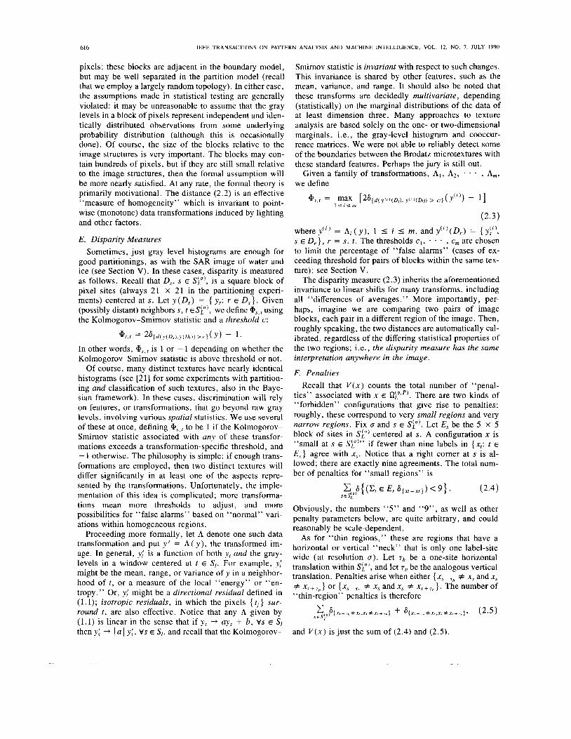
ties’’ associated with x E np9‘). There are two kinds of “forbidden” configurations that give rise to penalties: roughly, these correspond to very small regions and very narrow regions. Fix r~ and s E Sp). Let E, be the 5 x 5 block of sites in Sp) centered at s. A configuration x is “small at s E SF)” if fewer than nine labels in { x,: t E E,} agree with x,. Notice that a right comer at s is allowed; there are exactly nine agreements. The total number of penalties for “small regions” is

(2 .4)

Obviously, the numbers “5” and “9”, as well as other penalty parameters below, are quite arbitrary, and could reasonably be scale-dependent.

As for “thin regions,” these are regions that have a horizontal or vertical “neck” that is only one label-site wide (at resolution a). Let 7 h be a one-site horizontal translation within Sp), and let 7, be the analogous vertical translation. Penalties arise when either { xSpr , , # x, and x, # x, + T,, } or { x, - rl, # x, and x, # x, + r l , } . The number of ‘ ‘thin-region’’ penalties is therefore

(2 .5)

and V ( x ) is just the sum of (2.4) and (2.5).

GEMAN er al. : BOUNDARY DETECTION BY CONSTRAINED OPTIMIZATION 617

G. Summary 0 0 0

We are given I ) a gray-level image y = { yi j >; 2) a resolution u = 1 ,2 , * * - , and a maximum number

3) a disparity measure CP,,,( y ) for each pair ( s, t ), in

4) a collection of penalty patterns. The (MAP) partitioning .2 = a( y ) is then any solution

x E QfP,‘) of the constrained optimization

of labels P ;

the sublattice Sfp’;

where V ( x ) is the number of penalties in x.

111. BOUNDARY MODEL A . Boundary Maps

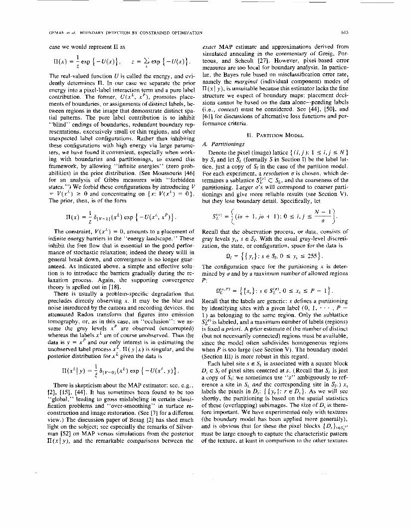
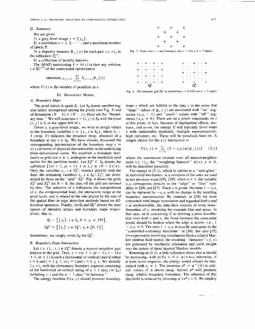
The pixel lattice is again SI . Let S, denote another regular lattice interspersed among the pixels (see Fig. 3) and of dimension ( N - 1 ) X ( N - 1 ); these are the “boundary sites.” We will associate s = ( i , j ) E S, with the pixel ( i , j ) E SI to the upper left of s.

Given y , a gray-level image, we wish to assign values to the boundary variables x = { x,, s E S , } , where x, = 1 (resp. 0) indicates the presence (resp. absence) of a boundary at site s E S,. We have already discussed the corresponding interpretation of the boundary map x = x ( y ) in terms of physical discontinuities in the underlying three-dimensional scene. We establish a boundary resolution or grid size a 2 1, analogous to the resolution used earlier for the partition model. Let Sg) C SB denote the sublattice { ( i u + 1 , j u + 1 ) : 1 5 i , j 5 ( N - 2 ) / u } . Only the variables x,, s E Sfp’, interact directly with the data; the remaining variables x,, s E S, \ Sg), are deter- mined by those on the “grid” Sfp’. Fig. 4 shows the grids Sh2) and Sb3’ for N = 8; the sites off the grid are denoted by dots. The selection of a influences the interpretation of x, the computational load, the interaction range at the pixel level, and is related to the role played by the size of the spatial filter in edge detection methods based on differential operators. Finally, let Q I and Q g ) denote the state spaces of intensity arrays and boundary maps respectively; that is,

QI = { { y s } : s € S I , 0 5 ys 5 2551,

n p = { (x,}: s E sp, x, E (0, I } } .

Sometimes, we simply write Q, for fig’.

B. Boundary-Data Interaction Let ( s, t ),, s, t E Sfp’ denote a nearest-neighbor pair

relativetothegrid. Thus,s = ( i u + l , j a + 1 ) , t = ( k a + 1, la + 1 ) is such a (horizontal or vertical) pair if either i = k a n d j = I ? 1, o r j = I and i = k +_ 1 . We identify ( s, t ), with the elementary boundary segment consisting of the horizontal or vertical string of u + 1 sites (in S,) including s, t and the u - 1 sites “in between.”

The energy function U ( x , y ) should promote boundary

+ + + +

0 0 0

0 0 0

Fig. 3 . Pixel sites ( O ) and boundary sites ( + ) for a 3 x 3 lattice

+ . + ’ + ’ + + . . + . . + + . + . + . + . . . . . . . + ‘ . + . ’ + . . . . . . . . . . . . . .

. . . . . . .

+ . + . + . + + ’ + . + . + . . . . . . .

. . . . . . .

. . . . . . . + . . + . . +

Sp

Fig. 4. The boundary grid S‘,.’ at resolutions U = 2 (left) and U = 3 (right).

maps x which are faithful to the data y in the sense that “large” values of As, , ( y ) are associated with “on” segments (x,x, = I ) and “small” values with “off” segments (x,x, = 0). There are no a priori constraints on x at this point; in fact, because of digitization effects, textures, and so-on, the energy U will typically favor maps x with undesirable deadends, multiple representations, high curvature, etc. These will be penalized later on. A simple choice for the x / y interaction is

u ( x , Y > = ( 1 - xsxr)$(A,. ,(Y)> (3.1) (S,f)O

where the summation extends over all nearest-neighbor pairs (s, t ) , ; the “weighting function” +(x) , x 1 0, will be described presently.

The energy in (3. l ) , which is similar to a “spin-glass” in statistical mechanics, is a variation of the ones we used in our previous work [19], [20]; when a = 1 , the variable xsxr corresponds directly to the “edge” or “line” variables in [20] and [47]. Since y is given, the term 1 - x , ~ , can be replaced by -x ,xr with no change in the resulting boundary interpretation. By contrast, in [20] we were concerned with image restoration and regarded both x and y as unobservable; the data then consists of some transformation of y , involving for example blur and noise. In that case, or in conceiving U as defining a prior distribution over both y and x, the bond between the associated pixels should be broken when the edge is active, i.e., 1 - x,x, = 0. The term 1 - x,xt is exactly analogous to the “controlled-continuity functions” in [56]. See also [35] for experiments involving simulations from a related Mar- kov random field model; the resulting “fantasies” ( y , x ) are generated by stochastic relaxation and yield insight into the nature of these layered Markov models.

Returning to (3. I ) , a little reflection shows that 4 should be increasing, with 4 (0) < 0 < $ ( + m ) ; otherwise, if $ were never negative, the energy would always be minimized with x, 3 1. The intercept d* = $ - ‘ ( O ) is critical; values of A above (resp. below) d* will promote (resp. inhibit) boundary formation. The influence of this threshold is reduced by choosing 4’ ( d ” ) = 0. We employ

618 IEEE TRANSACTIONS ON PATTERN ANALYSIS AND MACHINE INTELLIGENCE, VOL. 12. NO. 7. JULY 1990

the simple quadratic

Notice that if we select (Y = max A,y,, then the maximum “penalty” (+ ( 0 ) = - 1 ) and “reward” (+ (a) = 1 ) are balanced.

C. Disparity Measures We employ one type of measure for depth and shape

boundaries and another for the texture experiments. In the former case, the disparity measure involves the (raw) gray-levels only, whereas for texture discrimination we also consider data transforms based on the directional residuals (1.1). Except when U = 1, the data sets are compared by the Kolmogorov-Smimov distance.

The disparity measure should gauge the intensity “flux,” As, , = A$P,‘(y) 2 0 , across ( s , t ) , , i.e., orthog- onal to the associated segment. At the highest resolution ( U = l ) , the measure 1 ys, - y,, 1 (where s*, t* are the two pixels associated with the boundary sites s, t-see Fig. 5) can be effective for simple scenes but necessitates a single differential threshold: differences above d* (resp. below d* ) promote (resp. inhibit) boundary formation. Typically, however, this measure will fluctuate consid- erably over the image, complicating the selection of d*. (Such is the case, e.g., for the “cart” scene, see Section V .) Moreover, this measure lacks any invariance properties, as will be explained below. A more effective measure is one of the form

where the sum extends over parallel edges ( s i , t i ) in the immediate vicinity of ( s, t ). Thus the difference I ys. - y , , 1 is “modulated” by adjacent, competing differences. The result is a spatially varying threshold and the distribution of As,t ( y ) across the image is less v@able than that of 1 ys , - y,* I . Choosing y = const. x A , where A is the mean (raw) absolute intensity difference over all (vertical and horizontal) bonds, renders As, , ( y ) invariant to linear transformations of the data; that is, As , , ( y ) = A s , , ( a y + 6 ) for any a , b.

At lower resolution, let D,, and D,, denote two adjacent blocks of pixels, of equal size and shape. An example is illustrated in Fig. 6 for the case of two square blocks of size 52 = 25 pixels which straddle a vertical boundary segment with U = 3 . Let y ( D , ) = { ys , s E D , } , r = s* , t*, be the corresponding gray-levels and set

As.,(Y> = d ( Y ( D S * ) > Y(D,*) )3 ( 3 . 4 )

where d is the Kolmogorov-Smirnov distance discussed in Section 11. This is the disparity measure used for the House and Ice Floe scenes (see Section V).

0 + + + 0 0

0 + Fig. 5 . P i x i pairs (:>’s) associated with horizontal and vertical boundary

segments.

0 0 0 0 0 0 0 0 0 0

+(SI 0 0 0 0 0 0 0 0 0 0

o o o o o D r . D.. o o o o o

0 0 0 0 0 0 0 0 0 0

0 0 0 0 0 +(t)

0 0 0 0 0

Fig. 6. Pixel blocks D,, and D,, associated with the boundary segment ( S,

t ) 3 .

One difficulty with (3.4) is that the distance between two nonoverlapping histograms is the maximum value, namely 1, regardless of the amount of separation. Thus, two constant regions differing by a single gray-level are as “far apart” as two differing by 255 levels. Thus, it is occasionally necessary to “desensitize” (3.4) for example by “smearing” the data or perhaps adding some noise to it; see Section V .

Raw gray-level data is generally not satisfactory for discriminating textures. Instead, as discussed in Section 11, we base the disparity measure on several data transformations, involving higher order spatial statistics, such as the directional residuals defined in (1.1). Given a family A, , A2, * * . , A, of these transforms (see Section II), a resolution U, and blocks D,,, D,* as above, define

A , , , ( y ) = max [ c ; ’ d ( y ‘ ” ( D , . ) , Y ( ~ ) ( D ~ * ) ] ( 3 . 5 )

where y ( ; ) = Ai ( y ) , 1 5 i I m , and y ( ’ ) ( D , ) = { y: ’ ) , s E D , } , exactly as in Section 11. Then A.v,,( y ) > d* (and, hence, +(As , , ( y ) ) > 0) if and only if d ( y ( i ) ( D . y * ) , y ( ‘ ) ( D , * ) ) 2 d*cj for some transform i . The thresholds c l , * - , c, are again chosen to limit “false alarms.” Finally, we note that (3.5) has the same desirable invariance properties as the measure constructed for partitioning (Section 11).

I s i s m

D . Penalties V ( x ) again denotes the total number of “penalties” as-

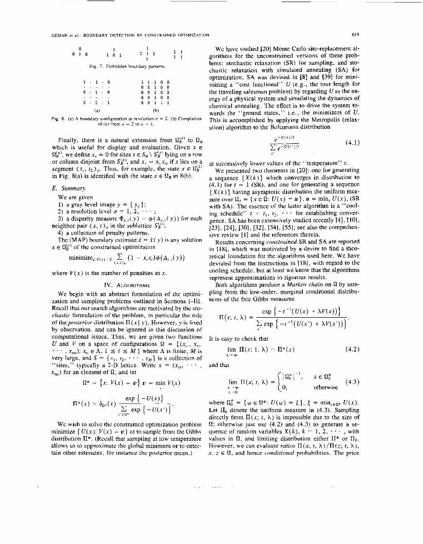
sociated with x E ap). These penalties are simply local binary pattems over subsets of S g ) . Fig. 7 illustrates a family of four such pattems; they can be associated with any resolution U by the obvious scaling. These correspond, respectively, to an isolated or abandoned segment, sharp turn, quadruple junction, and “small” structure. Depending on U, the pixel resolution, and scene information, we may or may not wish to include the latter three. For example, including the last one with U = 6 would prohibit detection of a square structure of pixel size 6 x 6.

GEMAN et al. : BOUNDARY DETECTION BY CONSTRAINED OPTIMIZATION 619

Fig. 7 . Forbidden boundary patterns.

1 . 1 . 0 1 1 1 0 0 0 0 1 0 0

0 . 1 . 0 0 0 1 0 0 0 0 1 0 0

0 ’ 1 . 1 0 0 1 1 1

(a) (b)

Fig. 8. (a) A boundary configuration at resolution U = 2. (b) Completion of (a) from U = 2 to U = 1.

. . . . .

. . . . .

Finally, there is a natural extension from Qg) to Q B

which is useful for display and evaluation. Given x E Qg), we define x, = 0 for sites s E SB \ S g ) lying on a row or column disjoint from S g ) , and x , ~ = xt,xt, if s lies on a segment ( t l , tz >,. Thus, for example, the state x E Qb2) in Fig. 8(a) is identified with the state x E Q B in 8(b).

E. Summary We are given 1) a gray-level image y = { y u } ; 2) a resolution level U = 1, 2, * * . ; 3) a disparity measure @,,t( y ) = +( As, t ( y ) ) for each

neighbor pair ( s, t >, in the sublattice S g ) ; 4) a collection of penalty patterns. The (MAP) boundary estimate i = i ( y ) is any solution

x E Qg) of the constrained optimization

minimizex:v(x)=o (1 - xsxt>+(As,r<Y>) ( s , r ) ,

where V(x) is the number of penalties in x.

IV. ALGORITHMS We begin with an abstract formulation of the optimi-

zation and sampling problems outlined in Sections 1-111. Recall that our search algorithms are motivated by the stochastic formulation of the problem, in particular the role of the posterior distribution n (x I y ). However, y is fixed by observation, and can be ignored in this discussion of computational issues. Thus, we are given two functions U and V on a space of configurations 52 = { (xs,, xs2, . . . , x,,): x,, E A, 1 s i I M } where A is finite, M is very large, and S = { sl, s2, * , sM} is a collection of “sites,” typically a 2-D lattice. Write x = (x,,, . . . , xsM) for an element of Q, and let

Q* = {x: ~ ( x ) = U } v = min ~ ( x ) X

exp { -w} I I * ( x ) = &*(x) C exp { -~(xj)}.

X ’ € i 2 *

We wish to solve the constrained optimization problem minimize { U ( x ) : V ( x ) = U } or to sample from the Gibbs distribution IT*. (Recall that sampling at low temperature allows us to approximate the global minimum or to entertain other estimates, for instance the posterior mean.)

We have studied [20] Monte Carlo site-replacement algorithms for the unconstrained versions of these problems: stochastic relaxation (SR) for sampling, and stochastic relaxation with simulated annealing (SA) for optimization. SA was devised in [8] and [39] for mini- mizing a “cost functional” U (e.g., the tour length for the traveling salesman problem) by regarding U as the energy of a physical system and simulating the dynamics of chemical annealing. The effect is to drive the system to- wards the “ground states,” i.e., the minimizers of U . This is accomplished by applying the Metropolis (relaxation) algorithm to the Boltzmann distribution

(4.1 )

at successively lower values of the “temperature” t . We presented two theorems in 1201: one for generating

a sequence { X ( k ) } which converges in distribution to (4.1) for t = 1 (SR), and one for generating a sequence { X ( k ) } having asymptotic distribution the uniform measure over Q, = (x E Q: U ( x ) = U}, U = minx U ( x ) , (SR with SA). The essence of the latter algorithm is a “cooling schedule” t = t , , t2 , - - * for establishing convergence. SA has been extensively studied recently [4], [lo], [23], 1241, [30], 1321, 1341, [ 5 5 ] ; see also the comprehen- sive review [ l ] and the references therein.

Results concerning constrained SR and SA are reported in [18], which was motivated by a desire to find a theoretical foundation for the algorithms used here. We have deviated from the instructions in 1181, with regard to the cooling schedule, but at least we know that the algorithms represent approximations to rigorous results.

Both algorithms produce a Markov chain on Q by sampling from the low-order, marginal conditional distributions of the free Gibbs measures

exp { - t - ’ ( U ( x ) + A V ( ~ ) ) }

C X ’ exp { - t - ’ ( U ( x ’ ) + A V ( ~ ’ ) ) ) ‘ n(x; t , A ) =

It is easy to check that

lim n(x; 1 , A ) = IT*(x) X + W

(4.2)

and that

lim n(x; t , A ) = (4.3) A - 0 , otherwise t-0

where 52: = {a E Q*: U(o) = E } , ,$ = minx,,* U ( x ) . Let IIo denote the uniform measure in (4.3). Sampling directly from I I ( x ; t , A ) is impossible due to the size of Q; otherwise just use (4.2) and (4.3) to generate a sequence of random variables X ( k ) , k = 1 , 2, * , with values in Q , and limiting distribution either II* or no. However, we can evaluate ratios n ( x ; t , A ) / I I ( z ; t , A ) , x, z E 52, and hence conditional probabilities. The price

620 IEEE TRANSACTIONS ON PATTERN ANALYSIS AND MACHINE INTELLIGENCE, VOL. 12. NO. 7. JULY 1990

for indirect sampling is that we must restrict the rate of growth of X and the rate of decrease o f t .

Fix two sequences { t k } , { A,}, a “site visitation” schedule { A k } , Ak C S, and let &(x) = n ( x ; tk, X k ) . The set Ak is the cluster of sites to be updated at “time” k; the “centers” of the clusters are addressed in a raster scan. In our experiments we take either I Ak 1 = 1 or 1 Ak 1 = 5,inwhichcasetheAk’sareoftheform { ( i , j ) , ( i + 1 , j ) , ( i - l , j ) , ( i , j + 11, ( i , j - I ) } .

Define a nonhomogeneous Markov chain { X( k) , k = 0, 1, 2, - } on Q as follows. Put X(0) = q arbitrarily. Given X(k) = (X,,(k), , XsM(k)), define X,(k + 1 ) = X , ( k ) f o ~ - s $ A ~ + ~ a n d l e t {X,(k + l ) : s ~ A ~ + ~ } b e a (multivariate) sample from the conditional probability distribution I&+l(x,, s E A k f l Ix, = X,(k), s 6 & + I ) . Then, under suitable conditions on { tk } and { hk} , either

lim P(X(k) = x ( X ( 0 ) = q ) = II*(x)

or the limit is IIo(x). The condition in the former case (constrained SR) is that tk = 1, X k 7 03, and X k 5 const.

log k. The condition for convergence to no (constrained SA) is that tk \1 0, X k 7 03 and tk lXk I const. * log k. The algorithm yields a solution to the constrained optimization problem (1.2) in the sense that the asymptotic distribution of X ( k) is uniform over the solution set: if the solution is unique, i.e., Cl,* = {xo}, then X(k) -+ xo in probability. See [ 181 for proofs.

k + m

A. Approximations The logarithmic rate is certainly slow. Still, we often

adhere to it for ordinary annealing; others [36] , [47] have as well. We refer the reader to [35] for some interesting comparisons between schedules. It is commonplace to find linear ( t k = to - a k ) and exponential ( tk = ( 1 - ~ ) ~ t ~ , y small) schedules; here k refers to the number of sweeps or iterations of S; in our experiments s = sP’ or sP’.

We now describe several protocols used in our experiments. One variant we do not use is to fix X k = X very large and do ordinary annealing, which might appear sen- sible since the solutions to min { U ( x ) : V ( x ) = 0} co- incide with those of min { U ( x ) + h V ( x ) } for all X suf- ficiently large (due to the fact that Q is finite). However this is not practical: unless to is very large and tk is reduced very slowly, the system immediately gets stuck in local energy minima of U + AV which are basically independent of the data, although faithful to the constraints. It is better to begin with states faithjid to the data and slowly impose the constraints, a standard technique in conventional optimization.

One variation of constrained SR that has been effective is “low-temperature sampling”: fix tk = E (small) and let X k 7 03. The idea is to reach a likely state of the posterior distribution II (x I y ) . In practice, we allow X k to grow linearly; the details are in Section V.

Another variation is the analog for constrained relaxation of “zero-temperature’’ sampling, which has been extensively studied by Besag [2] under the name ICM (for “iterated conditional modes”); see also [ 1 11, [ 141, and [22]. Without constraints, this algorithm, which is deterministic, results in a sequence of states X(k) which monotonically decrease the global energy, i.e. , increase the posterior likelihood. The constrained version operates as follows. Recall that when the set of sites Ak + is visited for updating, we defined X( k + 1 ) by replacing the co- ordinates of X(k) in Ak+ l by a sample drawn from the conditional distribution of I l k + on { x,, s E Ak + } given the values { x, = X, ( k ) , s 6 Ak + } . Suppose we replace the sample with the mode, i .e., the most likely vector { x,, s E Ak + } conditional upon { x, = X, ( k ) , s g! Ak + I }. In essence, we fix tk = 0 . This generates a deterministic se- quenceX(k), k = 0, 1, 2, * - - depending only onX(O), nk, and { A k } . (Notice that the mode is unaffected by t k since it corresponds to the minimum of U ( x) + X k V ( x). ) Then, during the kth sweep, with X = X k , the energy U + X k I/ is successively reduced, just as in ICM where hk = 0. Of course since there is nojixed (reference) energy, the algorithm cannot be conceived as one of iterative improvement. Several experiments were run with both the stochastic and deterministic algorithms; see Section V.

B. Summary Each experiment used one of the following two varia-

tions on constrained relaxation (see Section V for details): Choose a label resolution U and an associated pixel

block size. Select features. Choose a site visitation schedule { A k } , Ak C S k =

Fix a Zinear growth schedule for { X k } . Choose X(O), arbitrary. Set k = 0.

Deterministic Algorithm: 0) Set tk = 1, k = 1, 2, - 1) Define X,(k + 1 ) = X,(k), s $ A k + l and define

{ X, ( k + 1 ): s E Ak + } to be the (multivariate) mode of

1 , 2 , * . - .

* .

nk+l (Xs ,SEAk+l (xs = X,(k), S $ A k + l ) .

2) k = k + 1. 3) Go to 1. Stochastic Algorithm: 0) Set tk = E , k = 1, 2, * ( E “small”). 1) Define X,y ( k + 1 ) = X,y ( k ) , s 6 Ak + and define

{ X, ( k + 1): s E Ak + } to be a (multivariate) sample from

I I k + I ( x , J E A k + l I ~ , = X s ( k ) , s g ! A k + I ) .

2) k = k + 1. 3) Go to 1. Usually, but not always, the deterministic algorithm

was sufficient (again, see Section V).

GEMAN et al. : BOUNDARY DETECTION BY CONSTRAINED OPTIMIZATION 62 1

v. EXPERIMENTS’

A . Partition Model There are three experiments: an L-band synthetic ap-

erture radar (SAR) image3 of ice floes in the ocean (Fig. 9), a texture mosaic constructed from the Brodatz album [6] (Fig. lo), and another mosaic from pieces of rug, plastic, and cloth (Fig. 11).

Processing: In each experiment the partitioning was randomly initiated; the labels, x,s E Sp), were chosen in-

Thereafter, label sites were visited and updated one at a time, by a “raster scan” sweep through the label array. MAP partitionings were approximated by “zero-temperature” sampling (see Section IV), with X = X k increasing with the number of sweeps. Specifically, X was held at 0 through the first 10 sweeps, and thereafter was raised by 1 every 5 sweeps: hk = 0, k = 1, lo ; Xk = 1, k = 11, . 15; X k = 2, k = 16, - 20; etc. Most probably, A could have been increased more rapidly, perhaps with every sweep, without substantially changing the results, but this was not systematically investigated. For the three experiments shown in Figs. 9, 10, and 11, between 15 and 50 sweeps sufficed to bring the changes in labels to a halt; see below for more details. Recall that zero-temperature sampling corresponds to choosing the conditional mode. Occasionally there are ties, and these were re- solved by choosing randomly, and uniformly, from the collection of modes.

As a general rule, results were less reliable at higher resolutions (lower a’s) and when more labels were allowed (higher values of P ). In these cases, repeated experiments, with different initializations, often produced different results. With P too large, homogeneous regions were frequently subdivided, being assigned two or three labels. With U too small, the tendency was to mislabel small patches within a given texture. It is likely that many of these mistakes correspond to local minima; perhaps some could be corrected by following a proper annealing schedule (see Section IV), and by more careful choices of thresholds (see below). Here again, definitive experiments have not been done.

Measures of Disparity: Recall that the disparity measure is derived from the Kolmogorov-Smirnov distance between blocks of pixel data under various transformations, as defined in Section 11, equation (2.3). For the SAR image, good partitionings were obtained using only the raw data: m = 1 and y ( l ) is just y in (2.3). Evidently, gray-level distributions are enough to segment the water and ice “textures,” at least when supplemented by the “prior constraints” embodied in the penalty term V ( x ) .

dependently and uniformly from 0, 1, - - , P - 1.

’Fortran code and terminal sessions are available. ’We are grateful to the Radar Division at ERIM for providing us with

the SAR image (collected for the U.S. Geological Survey under Contract 14-08-0001-21748 and the Office of Naval Research under Contract N- 00014-81-C-0692 and N-00014-81-C-0295).

The texture collages in Figs. 10 and 11 are harder. We used four data transformations in addition to the raw pixel data. Hence, for these experiments m = 5, yc l ) = y, and y ( * ) , * - y(5) are based on various transforms. In particular,

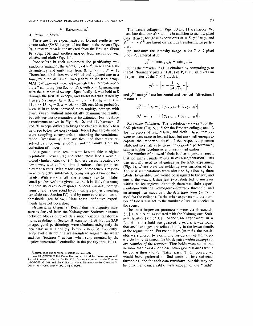
y;” measures the intensity range in the 7 x 7 pixel block V, centered at s:

maxtevSYr - minteV,Yr; y1*’ =

yf” is the “residual” (1.1) obtained by comparing y , to the 24 “boundary pixels” (dV,) of V, (i.e., all pixels on the perimeter of the 7 x 7 block):

yl” =

and y‘4’ and y(5) are horizontal and vertical “directional residuals” :

Parameter Selection: The resolution (a ) was 7 for the SAR picture (Fig. 9); 15 for the Brodatz collage; and 13 for the pieces of rug, plastic, and cloth. These numbers were chosen more or less ad hoc, but are small enough to capture the important detail of the respective pictures while not so small as to incur the degraded performance, seen at higher resolutions and mentioned earlier.

The number of allowed labels is also important; recall that too many usually results in over-segmentation. This was actually used to advantage in the SAR experiment (Fig. 9), where there are evidently two varieties of ice. The best segmentations were obtained by allowing three labels. Invariably, two would be assigned to the ice, and one to the water. Using just two labels led to mistakes within the ice regions, although there was little experi- mentation with the Kolmogorov-Smirnov threshold, and no attempt was made with the data transforms ( m > 1 ) used for the collages. In the other experiments, the number of labels was set to the number of texture species in the scene.

The most important parameters were the thresholds, { ci} 1 I i I m, associated with the Kolmogorov-Smir- nov statistics [see (2.3)]. For the SAR experiment, m = 1, and the threshold was guessed, a priori; it was found that small changes are reflected only in the lesser details of the segmentation. For the collages ( m = 5 ), the thresholds were chosen by examining histograms of Kolmogo- rov-Smirnov distances for block pairs within homogeneous samples of the textures. Thresholds were set so that no more than 3 or 4 % of these intraregion distances would be above threshold (a “false alarm”). Of course, we would have preferred to find more or less universal thresholds, one for each data transform, but this may not be possible. Conceivably, with enough of the “right”

622 IEEE TRANSACTIOES ON PATTERN ANALYSIS AND MACHINE INTELLIGENCE. VOL. 12. NO 7. JULY 1Y90

(b) Fir . 9. (a) Synthetic aperture radar image of oceanic ice floes. (b) Evo-

lution of the label states from random initialization (upper left) to final partition (lower right).

transforms, one could set conservative (high) and nearly universal thresholds, and be assured that visibly distinct textures would be segmented with respect to at least one of the transforms. Recall that the disparity measure (2.3) is constructed to signal “different” when the distance between blocks, with respect to any of the transforms, exceeds threshold.

Fig. 9 (SAR): As mentioned earlier, three labels were used, with the expectation that the ice would segment into two regions (basically, dark and light). The resolution was U = 7, and the Kolmogorov-Smimov statistic was computed only on the raw data, so m = 1 . The threshold was cI = 0.15. The original image is 512 X 512 (the pixel resolution is about 4 by 4 m ) , but to avoid special treat- ment of the boundary, only the 462 X 462 piece shown in Fig. 9(a) was processed. The label lattice Sp) is 64 x 64. Fig. 9(b) shows the evolution of the partitioning during the relaxation. For display. gray levels were arbitrarily assigned to the labels. The upper left panel is the random starting configuration. In successive panels are the states of the labels after each five iterations (full sweeps). In the bottom right panel, the two labels associated with ice are combined, “by hand.” Fig. 10 (Brodurz Textures): The Kolmogorov-Smirnov

thresholds were c I = 0.40, c2 = 0.53, c3 = 0.26. c4 = 0.28, and cs = 0.19, corresponding to the transforms 4.‘ I ,

* y”) discussed above. A 246 X 246 piece of the orig-

(b) Fig. 10. (a) Collage of five Brodatz textures. (b) Evolution of the labels.

upper left to lower right.

inal 256 X 256 image was processed, and is shown in Fig. 10(a). Leather and water are on top, grass and wood on the bottom, and sand is in the middle. The resolution was CJ = 15, which resulted in a 16 x 16 label lattice SP). Fig. 10(b) shows the random starting configuration (upper left panel), the configuration after 5 iterations (upper right panel), after 10 iterations (lower left panel), and after 15 iterations (lower right panel), by which point the labels had stopped changing.

Fig. 11 (Rug, Plastic, Cloth): The 216 X 216 image in Fig. 1 I(a) was partitioned at resolution CJ = 13, with a 16 x 16 label lattice. The Kolmogorov-Smirnov thresholds were c , = 0.90, c2 = 0.49, ci = 0.20, c4 = 0.11, and c5 = 0.12, corresponding to the same data transforms used for the Brodatz textures (Fig. 10). The experiment makes apparent a huzurd of long range bonds: the gradual but marked lighting variation across the top of the image produces a large Kolmogorov-Smimov distance when raw pixel blocks from the left and right sides are compared. This makes it necessary to essentially ignore the raw data Kolmogorov-Smirnov statistic, and base the partitioning on the four data transformations; hence the threshold cI = 0.9. The transformed data are far less sensitive to lighting gradients. Fig. 1 l(b) displays the evolution of the partitioning during relaxation. The layout is the same one used in the previous figures, showing every 5 iterations. except that there are 10 iterations between the final two

GEMAN ef U / BOUNDARY DETECTION BY CONSTRAINED OPTIMIIATION 623

(b)

bels. upper left to lower right. Fig. 1 1 . (a) Texture collage: rug, plastic. cloth. (h ) Evolution of the la-

panels. The lower right panel is the partitioning after the 30th sweep, by which time the pattern was “frozen.”

B. Bounday Model There are five test images: one made indoors from tin-

ker toys (“cart”), an outdoor scene of a house, another of ice floes in the ocean (the same SAR image used above), and two texture mosaics constructed from the Brodatz album.

Processing: All the experiments were performed with the same site-visitation schedule. Given the resolution U.

which varies among experiments, the sites of the sublattice Sf’ were addressed in a raster-scan andjive sites were simultaneously updated. Specifically, at each visit to the site (io + 1 , j o + 1 ), the values of the boundary process at this site and its four nearest neighbors, { ( ( i 1 ) U + 1 , ( j k 1 ) U + 1 ) }, were replaced based on the conditional distribution of these five boundary variables given the variables at the other sites and the data J. Of course this distribution is concentrated on the 2s = 32 possible configurations for these five variables.

Two update mechanisms were employed: stochastic relaxation and the “zero-temperature,” deterministic variation discussed earlier. In the former case, the updated binary quintuple is a sample from the aforementioned conditional distribution, which varies depending on the penalty weight AL for the kth sweep of the lattice SF ’ . Of course “O-temperature” refers to replacing the sample by

the conditional model. In both cases we let Ak grow linearly.

Stochastic relaxation at low temperature is more effective than at zero temperature (essentially iterative improvement). However, deterministic relaxation sufficed for all but two scenes, the ice floes and the four texture collage; these results could not be duplicated with deterministic relaxation. In one case, we present both results for comparison.

Generally, deterministic relaxation stabilizes in 5- 10 sweeps whereas stochastic relaxation requires more sweeps, perhaps 20-60. We provide several pictures showing the evolution of the algorithm.

Penalties: All the experiments were conducted with the same forbidden patterns, namely those in Fig. 12, with the exception of the house scene, for which the last pattern was omitted. (At the resolution used for the house, namely U = 3, the inclusion of that pattern would inhibit the formation of structures at the scale of six pixels; many such nontrivial structures appear in that scene.) Thus, the penalty function V ( x ) records a unit penalty for each oc- currence in the boundary map x = { xI , s E S g ) } of any of the five patterns depicted in Fig. 12. It is interesting to note that in no case was the final labeling completely free of penalties, i .e., V ( a ) = 0. Perhaps this could be achieved with a proper annealing schedule, or with up- dates of more than five sites.

Measures of Disparity: All the experiments are based on instances of the measures (3.3)-(3.5) described in Sec- tion 111.

1 ) For the first experiment, the cart scene, the boundary resolution is U = 1 and we employed the measure given in (3.3) with y = l O A and the raw difference 1 y,,. - y,*l modulated by the four nearest differences of the same orientation as ( s*, t* ) . Thus, for the horizontal pair ( s, t ) of adjacent boundary sites,

where s* = ( i , j ) , t* = ( i + 1 , j ) , and is the mean absolute intensity difference over the image. The utility seems largely impervious to the choice of the scaling constant (here = 10) for the mean as well as to the range of the modulation.

2) We used the Kolmogorov-Smirnov measure (3.4) for both the house and ice floes scenes. For the house, we chose U = 3 and blocks of size 25: the setup is depicted in Fig. 6. Due to the uniform character of the background (e.g., the sky) the distance (3.4) was computed based on the transformed data yIi = j I , + qr,, where { q r J } are independent variables, and distributed with a triangular density, specifically that of 1O(u , + U ? ) , u l , U ? uniform (and independent) on [ 0, 1 1.

The boundary resolution for the radar experiment is U

= 8. reflecting the larger important structures there; the image is 512 x 512. The dynamic range is very narrow

624 IEEE TRANSACTIONS ON PATTERN ANALYSIS AND MACHINE INTELLIGENCE, VOL. 12. NO. 7, JULY 1990

1 1 1 1

1 1 1 1 0 1 1 1 1

1 1 1

0 0 1 0

Fig. 12. Forbidden patterns for the boundary experiments.

and the difference between the dark water and somewhat less dark ice is essentially one of texture, due in part to the customary speckle noise. In particular, the ice cannot be well-differentiated from the water based on shading alone. The disparity measure is (3.4), applied to the raw image data over 24 x 24 blocks. The problem encoun- tered in the house scene is actually alleviated by the speckle.

3) The texture mosaic experiments are based on the measure (3.5) for a particular family A I , * , A5 of five data transformations or “features.” In each case, the resolution is U = 5 and block size is 21 X 21. Recall that these five features are combined into a single measure of change according to the formula in (3.5). The transformations used are the range

maxtc V, Yt - mints V, Yt Zjl’ =

over a 7 x 7 window Vs centered at pixel s, and the four directional residuals

These residuals were then uniformly averaged over V,, yielding the final features y ( ’ ) ,

It is instructive to compare the Kolmogorov-Smimov differences for the raw and transformed data over these texture mosaics. Typically, if one looks at the resulting two histograms of differences for a give transform, on finds that, whereas the raw (Kolmogorov-Smimov) differences are actually larger at the texture borders, the transitions between the borders and interiors are sharper for the transformed data. Detecting the boundaries with the raw data necessitates an unacceptable number of “false alarms” in the sense of interior “microedges.”

Finally, the values of the constants c I , . . * , c5 used in the construction of As,, [see (3.5)] are selected by restricting the percentage of false alarms. The details are given in the following section.

Parameter Selection: Recall that the total change across the boundary segment ( s , t ) is measured by 4 ( As,r( y ) ) , where 4 is given in (3.2). Given A, there are two parameters to choose: a normalizing constant a and the intercept d* = 4-’(0).

For the object boundary experiments, namely the cart,

* * Y ‘ ~ ) .

house, and ice floes, the parameters a and d* were chosen as follows. Find the mean disparity over all (vertical and horizontal) values of As,, for relevant bonds ( s, t ); take a equal to the 99th percentile of those above the mean and d* equal to the 70th percentile of those above the mean. This yields the values cy = 150, d* = 42 for the cart scene; recall that for this experiment, both the grid and block sizes are unity. For the house scene ( (T = 3 ) the Kolmogorov-Smimov statistics were computed over 5 X 5 blocks, and the resulting parameters are then a = 1 and d* = 0.7. (The number of distances at (the maximum) value A = 1 was considerable. ) Finally, for the ice floes, the recipe above yielded a = 0.33, d* = 0.13.

Tuming to the experiments with texture mosaics, let C ; , k denote the normalizing constant in (3.5) for feature i , 1 I i 5 5 , and texture k , 1 I k c: K , where K is the number of textures in the mosaic. For each feature i and texture type k , we computed the histogram of the (combined vertical and horizontal) Kolmogorov-Smimov distances and selected Ci ,k = loo( 1 - y ) percentile of that histogram. Specifically, we took y = 0.01 for the two Brodatz collages. (Other experiments indicated that any (small) value of y will suffice, say 0 5 y I 0.03. ) Thus, 100( 1 - y ) % of the distances d ( y ( i ) ( D l ) , y ( ; ) (D2)) are below c ; , ~ within each texture type k . Now set c; = maxl s k s K ~ i , k , ensuring that at most k y ( lO0)X of the interior differences As,f ( y ) within the entire collage will exceed the threshold d* = 1. Finally, we put a = 2.

Fig. 13 (Cart Scene): Sixty sweeps of stochastic relaxation were run with t k * 0.05 and X p 7 3. Actually, all the boundaries were “in place” after about 10 sweeps, as illustrated in Fig. 13(b), which shows every third sweep up to the 46th. The image is 110 X 110. Not shown is a run with the deterministic algorithm; the results are vir- tually indistinguishable.

Fig. 14 (House Scene): This 256 X 256 monochrome image was supplied to us by the Visions group at the Uni- versity of Massachusetts. The update is by deterministic relaxation with X k increasing linearly from ho = 0 to X l o = 2.

Fig. 15 (Ice Floes): The image in Fig. 15(a) is 512 X 512. We did 60 sweeps of stochastic relaxation with t k = 0.1 and hk 7 2. Fig. 15(b) shows 16 “snapshots”- every third sweep as in Fig. 13, as well as the final (60th) sweep.

Fig. 16 (Brodatz Collage 1): The collage is composed of nine Brodatz textures [Fig. 16(a)]: leather, grass, and pigskin (top row), raffia, wool, and straw (middle row), and water, wood, and sand (bottom row). Two of the textures, leather and water, are repeated in the two circles. The image size is 384 x 384, the individual textures all being 128 X 128. We show the results [Fig. 16(b)] of both the deterministic (left) and stochastic (right) algorithms; they are roughly comparable. Other false alarm rates ( y = 0.005, 0.02, and 0.03) yield the same overall quality.

Fig. 17 (Brodatz Collage 2): There are four textures

GOMAN CI (11.: BOUNDARY I ~ I T I I K T I O N BY CONSTKAINEU OVIIML%AIION

(b)

Fig. 13. (a) Irnage a i il tinker toy c a r t (b) Evolution or the boundaries (upper lcfl to lowcr right) with moltiplc-sitc stochastic relaxation

625

(b)

Fig. 15. (a) Ice flocs imagc [sec Fig. 9(a)]. (h) Evalotinn of the boundaries (a t resolution LT = 8 ) during stochastic relaxiitinn.

Fig. 14 (b)

= 3 with deterministic relaxation. (a) House scenc. (h) Final boundary placcmenls at resolution c

(b)

Pig. 16. (a) Collage of nine Brodetz texturces. (b) Final boundary place- mcnts with deterministic relaxalion (Mi) and stochastic relaxatiun (right).

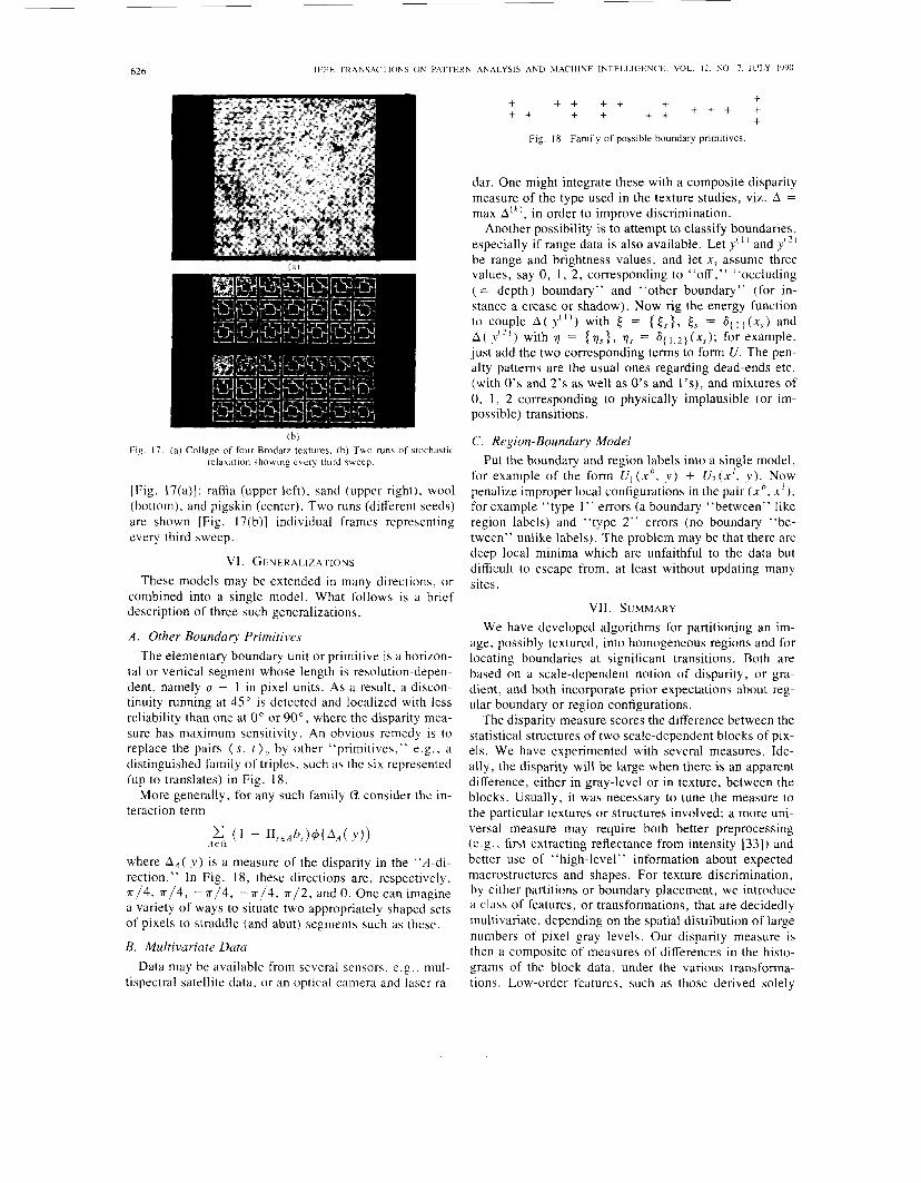
626 I E t P TRANSACTIOhS ON PATTERN ANALYSIS AND MACHINF IhTELLIGENCE. VOL 12. NO 7. JULY li)i)o

(b) Fig. 17. (a) Col lage of four Brodatz tex tures . (b) T w o runs of stochastic

relaxation showing every third s w e e p .

[Fig. 17(a)]: raffia (upper left), sand (upper right), wool (bottom), and pigskin (center). Two runs (diRerent seeds) are shown [Fig. 17(b)] individual frames representing every third sweep.

VI. GENERALIZATIONS These models may be extended in many directions, or

combined into a single model. What follows is a brief description of three such generalizations.

A . Other Boundary Primitives The elementary boundary unit or primitive is a horizon-

tal or vertical segment whose length is resolution-dependent, namely 0 + 1 in pixel units. As a result, a discontinuity running at 45” is detected and localized with less reliability than one at 0” or 90”, where the disparity measure has maximum sensitivity. An obvious remedy is to replace the pairs (s, r ) , by other “primitives,” e.g. , a distinguished family of triples, such as the six represented (up to translates) in Fig. 18.

More generally, for any such family a consider the interaction term

where A,( y ) is a measure of the disparity in the “A-direction.” In Fig. 18, these directions are, respectively, w / 4 , 7r/4, -w/4, - -w/4 , w / 2 , and 0. One can imagine a variety of ways to situate two appropriately shaped sets of pixels to straddle (and abut) segments such as these.

B. Multivariate Datu Data may be available from several sensors, e.g. , mul-

tispectral satellite data, or an optical camera and laser ra-

+ + + I + + + + + + + + +

+ + + + Fig . 18. Family of possible boundary primitives

dar. One might integrate these with a composite disparity measure of the type used in the texture studies, viz. A = max A ( k ) , in order to improve discrimination.

Another possibility is to attempt to classify boundaries, especially if range data is also available. Let y‘” and y‘” be range and brightness values, and let x, assume three values, say 0, 1, 2, corresponding to “off ,” “occluding ( = depth) boundary” and “other boundary” (for instance a crease or shadow). Now rig the energy function to couple A ( y ( ’ ) ) with 4 = { 4, }, 5, = 6, } ( x , ) and A ( $’)) with q = ( q s } , qs = 6i l ,2}(xs) ; for example, just add the two corresponding terms to form U . The penalty patterns are the usual ones regarding dead-ends etc. (with 0’s and 2’s as well as 0’s and l’s), and mixtures of 0, 1, 2 corresponding to physically implausible (or impossible) transitions.

C. Region-Boundary Model Put the boundary and region labels into a single model,

for example of the form U , ( X ’ , y ) + U 2 ( x ‘ , y ) . Now penalize improper local configurations in the pair (x’, x‘), for example “type 1 ” errors (a boundary “between” like region labels) and “type 2” errors (no boundary “between” unlike labels). The problem may be that there are deep local minima which are unfaithful to the data but difficult to escape from, at least without updating many sites.

VII. SUMMARY We have developed algorithms for partitioning an im-

age, possibly textured, into homogeneous regions and for locating boundaries at significant transitions. Both are based on a scale-dependent notion of disparity, or gradient. and both incorporate prior expectations about regular boundary or region configurations.

The disparity measure scores the difference between the statistical structures of two scale-dependent blocks of pixels. We have experimented with several measures. Ide- ally, the disparity will be large when there is an apparent difference, either in gray-level or in texture, between the blocks. Usually, it was necessary to tune the measure to the particular textures or structures involved; a more universal measure may require both better preprocessing (e.g., first extracting reflectance from intensity [33]) and better use of “high-level” information about expected macrostructures and shapes. For texture discrimination, by either partitions or boundary placement, we introduce a class of features, or transformations, that are decidedly multivariate, depending on the spatial distribution of large numbers of pixel gray levels. Our disparity measure is then a composite of measures of differences in the histograms of the block data, under the various transformations. Low-order features, such as those derived solely

627 GEMAN er 01. B O U N D A R Y DETECTION BY CONSTRAINED OPTlMlLATlON

from raw gray-level histograms and cooccurrence matrices, were not as effective i n our framework.

Disparity measures between pairs of pixel blocks drive the segmentations or boundary placements through a "label model, " that specifies likely label configurations conditional on disparity data. For partitioning, labels are generic and associated with local blocks of the image. Two labels are the same if their respective regions are judged to be instances of the same texture. For boundary placement, the labels are zero or one, and interpreted as indi- cating, respectively, the absence or presence of boundary elements. A priori knowledge about acceptable label configurations, which, for example, may preclude very small or thin regions, or cluttered boundary elements, is applied by restricting labels to an appropriate subset of all possible configurations. The result of modeling disparity-label interactions and of defining restricted configurations can be regarded as a Gibbs distribution jointly on pixel gray levels and label configurations, with the marginal label distribution supported on a subset of the configuration space.

Partitioning and boundary finding is accomplished by approximating the maximum a posreriori (MAP) label configuration, conditioned on observed pixel data. Be- cause certain configurations are forbidden, MAP estimation amounts to constrained optimization. Stochastic relaxation and simulated annealing are extended to accommodate constraints by introducing a nonnegative constraint function that is zero only for allowed label configurations. The constraint function, with a multiplicative constant, is added to the posterior energy, and the constant is slowly increased during relaxation. Straightfor- ward calculations establish an upper bound on the rate of increase of this multiplicative constant that ensures convergence of the relaxation and annealing algorithms to the desired limits. In a series of partitioning and boundary- finding experiments, deterministic and other fast varia- tions of the constrained relaxation algorithm are found to be effective.

The partitioning model is appropriate when a small number of homogeneous regions are present. Disjoint instances of a common texture are automatically identified. The boundary model can be effective in complex, multi- textured, scenes. Both models sometimes require prior training to adjust parameters.

ACKNOWLEDGMENT We are indebted to E. Bienenstock for recommending

the random topology employed in the partition model, and for pointing out a fascinating connection to some work in neural modeling [42].

REFERENCES [I] E. Arts and P. van Laarhoven. "Simulated annealing: A pedestrian

review of the theory and some applications." in N A 7 0 Adwrirecl Stud! Institlrte on Pattern Recognition: Theor! a r i d Applicatiorr\. Spa. Bel- gium. 1986.

121 J . Besag. "On the statistical analysis of ditty pictures" (with discussion). J . Roy. Statist. Soc. , series B, vol. 48, pp. 259-302. 1986.

[31 A. Blake, "The least disturbance principle and weak constidints." Partern Recog. Let t . , vol. I . pp. 393-399, 1983.

[4] E. Bonomi and J.-L. Lutton, "The n-city travelling salesman problem: Statistical mechanics and Metropolis algorithm," SIAM Re\%. , vol. 26. pp. 551-568, 1984.

[5] A. Brandt, "Multi-level approaches to large scale problems," in Proc. lnt. ConRr. Mathemariciuns 1986, A. M. Gleason, Ed., Amer. Math. Soc.. Providence. RI, 1987.

[6] P. BrodatL. Texture: A Phorographir Album f o r Artists and Desigr7- ers. New York: Dover, 1966.

171 T . M. Cannon, H. J . Trussell. and B. R. Hunt. "Comparison of image restoration methods," Appl . Opt. , vol. 17, pp. 3385-3390. 1978.

181 V. Cemy. "A thermodynamical approach to the travelling salesman problem: An efficient simulation algorithm," Inst. Phys. Biophys., Comenius Univ., Bratislava, Czechoslovakia, 1982.

(91 B. Chalmond, "Image restoration using an estimated Markov model," Dep. Math., Univ. Paris, Orsay, France. 1987.

IO] T.-S. Chiang and Y. Chow, "On eigenvalues and optimal annealing rate," Inst. Math., Academia Sinica, Taipei, Taiwan, preprint 1987.

I l l F. S. Cohen and D. B. Cooper, "Simple parallel hierarchical and relaxation algorithms for segmenting noncausal Markovian random fields." IEEE Trans. Pattern Anal. Machine Inrell., vol. PAMI-9.

121 H. Derin and W. S. Cole, "Segmentation of textured images using Gibbs random fields," Compur. Vision. Graphics, Image Processing, vol. 35. pp. 72-98, 1986.

[13] H. Derin and H. Elliott. "Modeling and segmentation of noisy and textured images using Gibbs random fields," IEEE Trans. Partern Anal. Machine Intell. , vol. PAMI-9. pp. 39-55. 1987.

(141 H. Derin and C. Won, "A parallel image segmentation algorithm using relaxation with varying neighborhoods and its mapping to array processors," Dep. Elec. Comput. Eng., Univ. Massachusetts, Tech. Rep.. 1986.

[I51 P. A. Devijver and M. M. Dekesel, "Learning the parameters of a hidden Markov random field image model: A simple example." in Pattern Recognition Theory and Applications. P. A . Devijver and J . Kittler. Eds.

[ 161 A . Gagalowicz and Song De Ma, "Sequential synthesis of natural textures." Cornput. Vision, Gruphics, Image Processing, vol. 30, pp. 289-315. 1985.

[I71 D . Geman. "A stochastic model for boundary detection," Image Vi- sion Cofnput., May 1987.

(181 D. Geman and S. Geman, "Relaxation and annealing with constraints." Division Appl. Math., Brown Univ., Complex Systems Tech. Rep. 35, 1987.

[I91 D. Geman, S . Geman, and C . Graffigne, "Locating texture and object boundaries." in Pattern Recognition Theor?. and Applications. P. A. Devijver and J Kittler, Eds. Heidelberg: Springer-Verlag. 1987.

[20] S. Geman and D. Geman, "Stochastic relaxation, Gibbs distributions. and the Bayesian restoration of images," IEEE Trans. Pattern Anal. Machine Inre//. . vol. PAMI-6, pp. 721-741. 1984.

( 2 I ] S. Geman and C . Graffigne. "Markov random field image models and their applications to computer vision," in Proc. Int. Congr. Marhe- maricians, 1986, A. M. Gleason, Ed., Amer. Math. Soc.. Provi- dence. RI. 1987.

1221 S. Geman and D. E. McClure. "Statistical methods for tomographic image reconstruction." in Bull. IS1 (Proc. 46th Session In t . Srarisri- ral Instirure), vol. 5 2 , 1987.

[23] B. Gidas. "Nonstationary Markov chains and convergence of the annealing algorithm," J . Statist. Phys . , vol. 39, pp. 73-131, 198.5.

1241 -. "A renormalization group approach to image processing problems," IEEE Truns. Puttern Anal. Machine Inrell., vol. 1 I . pp. 164- 180, Feb. 1989.

(251 C. Graffigne. "Experiments in texture analysis and segmentation," Ph.D. dissertation, Division Appli. Math., Brown Univ., 1987.

[26] P. J . Green. "Discussion on "On the statistical analysis of dirty pictures." J . Besag. J . Roy. Starisr. Soc. . vol. B-48. pp, 259-302. 1986.

[27] D. M. Greig, B. T , Porteous, and A. H . Seheult, Discussion on "On the statistical analysis of dirty pictures." by J . Besag. J . R o y Srutist.

1281 U . Grenander. "Tutorial in pattern theory." Division Appl. Math.. Brown Univ.. Lecture Notes Volume, 1984.

1291 W. E. L. Grimson and T . Pavlidis, "Discontinuity detection for visual surface reconstruction. " Compur. Vision. Graphics. Iinccjie Pro- cessing, vol . 30. pp, 316-330. 1985.

pp. 195-219. 1987.

Heidelberg: Springer-Verlag. 1987, pp. 141-163.

SOC.. vol. B-48. pp. 259-302, 1986.

628 IEEE TRAKSACTIONS ON PATTFRN AKALYSIS AND MACHINE INTELLIGENCF. VOL I?. NO 7. JULY IY90

[30] B. Hajek, “A tutorial survey of theory and applications of simulated annealing.” in Proc. 24rh /€€E Con$ Decisiori arid Control. 1985. pp. 755-760.

[31] R. M. Haralick. K. Shanmugam. and I . Denstein, “Textural features for image classification.” IEEE Trans. Sysr.. Man. Cyhrrn. , vol. 6 , pp. 610-621. 1973.

[32] R . Holley and D. Stroock. “Simulated annealing via Sobolev ine- qualities,” preprint. 1987.

(331 B. K . P. Horn and M. J . Brooks. “The variational approach to shape from shading,” Compur. Visioti. Graphics, Image ProcessinLy, vol. 33 , pp. 174-208, 1986.

[34] C.-R. Hwang and S.-J . Sheu. “Large time behaviors of perturbed diffusion Markov processes with applications.” I , 11, and I l l , Inst. Math., Academic Sinica, Taipei. Taiwan, preprint 1987.

[35] A. Kashko and B. F. Buxton, “Markov random fantasies.” preprint, 1986.

[36] A. Kashko, H. Buxton. and B. F. Buxton, “Parallel stochastic optimization in computer vision,” preprint, 1987.

[37] R. L. Kashyap and K. Eom. “Texture boundary detection based on the long correlation model,” /E€€ Trans. Pattern Anal. Machine In-

[38] R. L. Kashyap and A. Khotanzad. ”A model-based method for rotation invariant texture classification,” l€EE Trans. Parrern Anal. Machine ltirell. . vol. PAMI-8. pp. 472-481. 1986.

(391 S. Kirkpatrick, C. D. Gellatt, Jr . . and M. P. Vecchi, “Optimization by simulated annealing.” Science. vol. 220, pp. 671-680, 1983.

[40] K . Laws. “Textured image segmentation,” Ph.D. dissertation. Univ. Southern California, Los Angeles, USCIPl Rep. 940, 1980.

[41] R. Linsker, “An iterative-improvement penalty-function-driven wire routing system,” I E M J . Res. Dewlop.. vol. 28, pp. 613-624, 1984.

[42] C. von der Malsburg and E. Bienenstock. “Statistical coding and short-term synaptic plasticity: A scheme for knowledge representation in the brain, ’ ‘ in Disordered System and Biological 0rgani:a- rion (NATO AS1 Series), E. Bienenstock. F. Fajelman SouliC, and G. Weisbuch, Eds.

[43] J . L. Marroquin. “Surface reconstruction preserving discontinuities,” Artificial Intell. Lab., Massachusetts Inst. Technol., Memo 792. 1984.

[44] J. L. Marroquin, S. Mitter, and T. Poggio, “Probabilistic solution of ill-posed problems in computational vision,” J . Amer. Starisr. As- SOC., vol. 82, pp. 76-89, 1987.

[45] J . W. Modestino. R. W . Fries, and A. L. Vickers, “Texture discrimination based upon an assumed stochastic texture model.” IEEE Trans. Pattern Anal. Muchine Intell. , vol. PAMI-3. pp. 557-580. 1981.

[46] J. Moussouris. “Gibbs and Markov random systems with constraints,” J . Srarisr. Phys. , vol. 10. pp. 11-33. 1974.

[47] D. W. Murray and B. F. Buxton. “Scene segmentation froin visual motion using global optimization,” IEEE Trans. Parrern Anal. M a - chine I n t e l l . . vol. PAMI-9. pp. 220-228. 1987.

[48] T . Pavlidis, “A critical survey of image analysis methods.” Ex- panded version of paper delivered to 8th Int. Conf. Pattern Recogni- tion, Paris. France, Oct. 1986.

[491 T. Poggio, V. Torre, and C. Koch, “Computational vision and regularization theory.“ Narure. vol. 317. pp. 314-319, 1985.

[SO] B . D. Ripley, “Statistics. images. and pattern recognition.” Canu- dian J . Stati.sr., vol. 14, pp. 83-1 1 I , 1986.

(511 A. Rosenfeld and L . S. Davis. ”Image segmentation and image models,” Proc. I € € € . vol. 67, pp. 764-772, 1979.

[521 B. W. Silverman. Discussion on “On the statistical analysis of dirty pictures,” by J . Besag. J . Roy. Srutisr. Soc. . vol. 8-48. pp. 259-302. 1986.

[53] T . Simchony and R. Chellappa, “Stochastic and deterministic algorithms for texture segmentation,’’ Dep. EE-Syst.. Univ. Southern California, 1988.

[S4] R. H. Swendsen and J.-S. Wang. “Nonuniversal critical dynamics in Monte Carlo Fimulations,” Phys. Rev. Lett.. vol. 58. pp. 86-88, 1987.

[ 5 5 ] H. szu, “Non-convex optimization,” in Proc. SPIE Con$ Real Time Signal Processing f X , vol. 698, 1986.

1-56] D. Terzopoulos. “Regularization of inverse visual problems involving discontinuities.” fEEE Trans. Parrerri Anal. Machine /rite//. , vol. PAMI-8, pp. 413-424. 1986.

[571 W. B. Thompson. “Textural boundary analysis.“ f € E € Trans. Coni-

[58] E. E. Triendl, “Texturerkennung and texturreproduktion.” Kyher-

fell . . vol. PAMI-2, pp. 58-67, 1989.

Berlin: Springer-Verlag. 1986.

PU/.. vol. C-26, pp. 272-276. 1977.

nrtik, vol. 13, pp. 1-5. 1973.

[59] E. Triendl and T . Henderson. “A model for texture edges,” in Proc. 5th Int. Con,[ Parrerri Recognition, Miami Beach. FL, Dec. 1-4.

[60] H. L. Voorhees, Jr.. “Finding texture boundaries in images.” Mas- ter’s thesis, Dep. Elec. Eng. Comput. Sci., Massachusetts Inst. Tech- nol.. 1987.

[61] W. A. Yasnoff, J. K. Mui, and J . W . Bacus, “Error measures for scene segmentation,” Parrern Recog., vol. 9, pp. 217-231, 1977.

1621 A. I . Zobrist and W. B. Thompson. “Building a distance function for Gestalt grouping.” I€€€ T r a m . Comput.. vol. C-24, pp. 718-728, 1975.

1980. pp. 1100-1 102.

Donald Geman (M’84) received the B.A. degree in English literature from the University of Illi- nois, Urbana, in 1965 and the Ph.D. degree in mathematics from Northwestern University, Ev- anston. IL. in 1970.

Since 1970 he has been a member of the De- partment of Mathematics and Statistics, Univer- sity of Massachusetts, Amherst. where he is currently Professor of Mathematics and Statistics. His visiting appointments include those at the Univer- sity of North Carolina (1976-1977), Brown Uni-

versity (1983), and UniversitC de Paris-Sud (1986). His research interests are in stochastic processes. image processing, and computer vision.

Stuart Geman (M’84) received the B.A. degree in physics from the University of Michigan, Ann Arbor, in 1971, the M.S. degree in physiology from Dartmouth College, Hanover, NH, in 1973. and the Ph.D. degree in applied mathematics from the Massachusetts Institute of Technology, Cam- bridge, in 1977.

Since 1977 he has been a member of the Di- vision of Applied Mathematics at Brown Univer- sity. Providence, RI, where he is currently Pro- fessor of Applied Mathematics. His research

interests include stochastic processes. image and speech processing. and computer vision.

Dr. Geman is a Fellow of the Institute of Mathematical Statistics and was a recipient of the Presidential Young Investigator Award.

Christine Graffigne was born in LiCvin. France, on December 1, 1959. She received the Master’s degree in mathematics from Lille University. France. in 1982. the French Ph.D. degree from Paris-Sud University, Orsay, France, in 1986, and the Ph.D. degree in applied mathematics from Brown University. Providence, RI. in June 1987.

From 1987 until 1988, she was an Assistant Professor at Paris-Sud University. Orsay. France. Since 1988. she has been a Research Scholar with the French National Center for Scientific Research

(CNRS), and has worked at Paris-Sud University. Her research interests are focused on stochastic processes. image processing. pattern recognition, and parallel computing.

Ping Dong (M’88) was born in Zhuzhou, China. on December 2, 1954. He received the B.S. and M.S. degrees in electrical engineering from Northwest Telecommunication Engineering Insti- tute, Xian, China, in 1979 and 1981, respectively. and the Ph.D. degree in electrical engineering from University of Massachusetts at Amherst in 1987.

He joined the Codex, Motorola research and advanced development department, Canton, MA, in 1987. His current research interests are image

segmentation and estimation algorithms, random signal processing and estimation algoriihms, and communication theory.

boundary detection by constrained optimization - · pdf fileieee transactions on pattern ......

Documents