iec 61000-4-3:2006 edition 3 standard update and how to select
TRANSCRIPT
IEC 61000-4-3:2006 Edition 3Electromagnetic compatibility (EMC) - Part 4-3 : Testing and measurementtechniques -Radiated, radio-frequency, electromagnetic field immunity test
Standard Update and how to select the correct amplifier
Jason H. SmithSupervisor Applications Engineerar rf/microwave instrumentation
160 School House Road Souderton, PA 18964-9990 [email protected]

New IEC 61000-4-3 Ed 3.0 is here!
J. Smith
Current document stages:Stage Meaning Actual Date Projected Date
CDIS Final Draft for final vote 11-4-05 11-30-05
APUB Approval of the Final Draft 1-13-06 2-28-06
BPUB Print of the Final Standard 2-07-06 3-31-06
PPUB Issue of the Final Standard
2-07-06 4-30-06
What does this mean?This IEC standard is accepted and its procedures need to
be used when called out by product standards. There is no stated overlap time period between releases
for IEC standards.
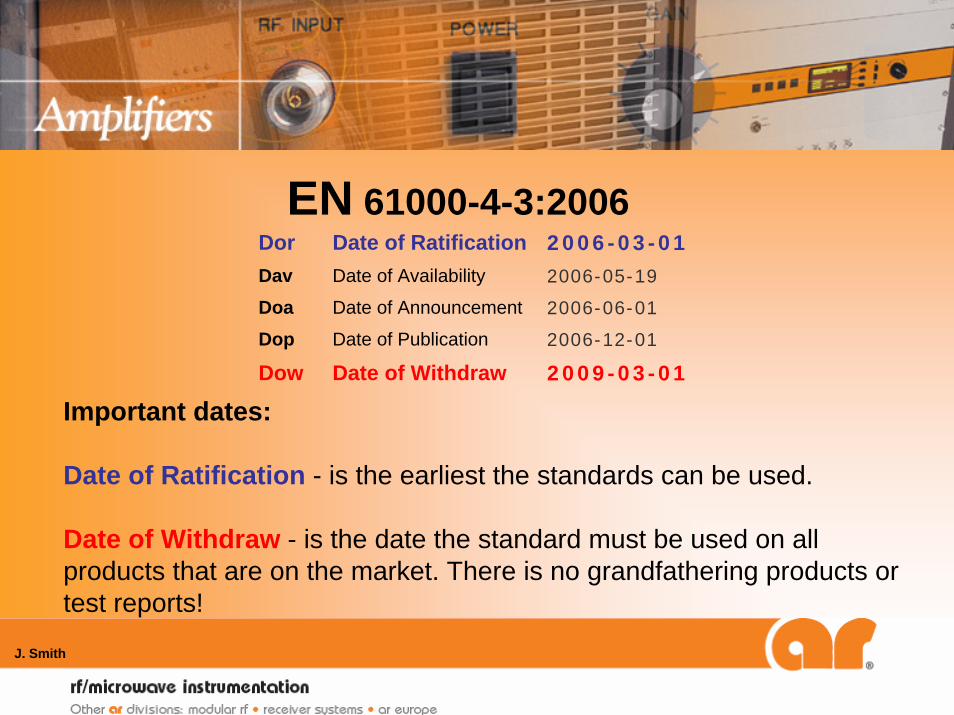
EN 61000-4-3:2006
J. Smith
Important dates:
Date of Ratification - is the earliest the standards can be used.
Date of Withdraw - is the date the standard must be used on all products that are on the market. There is no grandfathering products or test reports!
Dor Date of Ratification 2006-03-01Dav Date of Availability
Date of Announcement
Date of Publication
Date of Withdraw
2006-05-19
Doa 2006-06-01
Dop 2006-12-01
Dow 2009-03-01

Review:
IEC 61000-4-3 Test and measurement techniques – Radiated, radio-frequency, electromagnetic field immunity test
This is a individual test test standardProduct Standards will call out IEC 61000-4-3 and other test
standards. Example: IEC 61000-6-1 Generic Immunity standardProduct Standards state frequency range, levels, as well as,
any changes to the basic test standards.Product Standards take precedence over test standard.
Product standards require the latest test standard to be used
J. Smith

Why Care?
J. Smith
ManufacturersNeed to know the standards and keep informed when changes occur in order to keep track of product testing and when or ifretesting is required. Be aware of your test lab’s capabilities.
Independent Test Labs and Manufacturers Self TestingNeed to look ahead and think of the longevity of products tested so retesting is not needed in a few years.

Changes:
New check for linearity of amplifierNew requirement for harmonic distortion for Test
SetupsNew frequency range extending up to 6 GHzAbove 1 GHz smaller uniform field “windows” can be
used instead of the standard 1.5mx1.5mCalibration 1.8 x the needed field strengthNew low permeable material requirement for Test
Table
J. Smith
Requirement
J. Smith
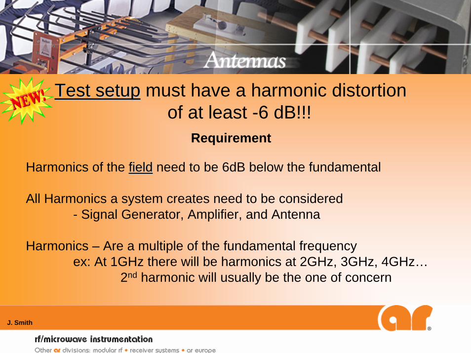
Test setupTest setup must have a harmonic distortion of at least -6 dB!!!
Harmonics of the fieldfield need to be 6dB below the fundamental
All Harmonics a system creates need to be considered - Signal Generator, Amplifier, and Antenna
Harmonics – Are a multiple of the fundamental frequency ex: At 1GHz there will be harmonics at 2GHz, 3GHz, 4GHz…
2nd harmonic will usually be the one of concern

Why is the new harmonic requirement necessary?
J. Smith
•When using a broadband receiving device for field calibration such as a field probe, it will not distinguish between different signals (fundamental or harmonic)
•High harmonics can contribute to the readings of the field probe and produce error in the reading.
•This error will cause testing at the intended fundamental frequency to be incorrect.
•If the harmonics are more then 6dB down from the fundamental in the chamber then there will be little error in the reading according to the standard.
Test setup must have a harmonic distortion of at least -6 dB!!!

Important considerations
J. Smith
•To predict what the harmonics will be in the chamber two main pieces of the system are of concern:
•Amplifier Harmonic content rating•This is a rating given by the amplifier manufacturer •This is what must be controlled for meeting this requirement
•Antenna Gain •Usually will increase throughout its frequency range.•For this reason the harmonic will have a higher gain than the fundamental
Test setup must have a harmonic distortion of at least -6 dB!!!
Test setup must have a harmonic distortion of at least -6 dB!!!
J. Smith
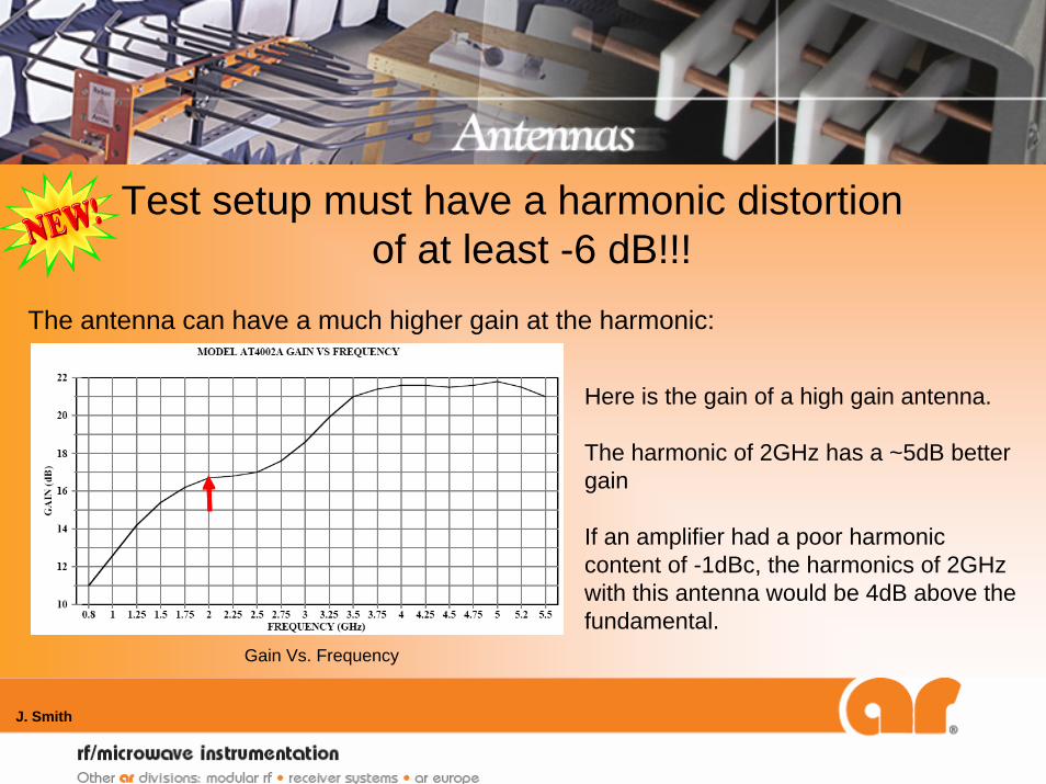
Gain Vs. Frequency
The antenna can have a much higher gain at the harmonic:
Here is the gain of a high gain antenna.
The harmonic of 2GHz has a ~5dB better gain
If an amplifier had a poor harmonic content of -1dBc, the harmonics of 2GHz with this antenna would be 4dB above the fundamental.
Test setup must have a harmonic distortion of at least -6 dB!!!
J. Smith
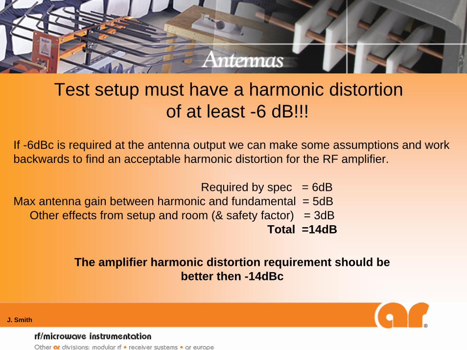
If -6dBc is required at the antenna output we can make some assumptions and work backwards to find an acceptable harmonic distortion for the RF amplifier.
Required by spec = 6dBMax antenna gain between harmonic and fundamental = 5dB
Other effects from setup and room (& safety factor) = 3dBTotal =14dB
The amplifier harmonic distortion requirement should be better then -14dBc

Check the amplifier manufactures' rating and available production data
J. Smith
25S1G4A
How to check test setup for harmonics
J. Smith
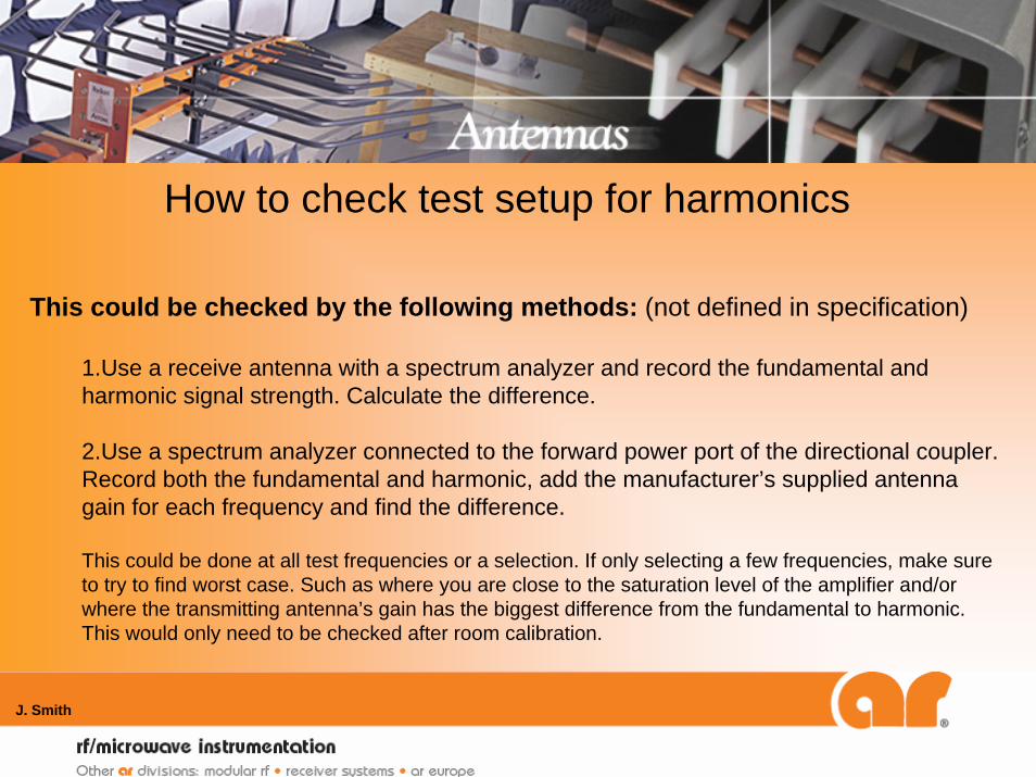
This could be checked by the following methods: (not defined in specification)
1.Use a receive antenna with a spectrum analyzer and record the fundamental and harmonic signal strength. Calculate the difference.
2.Use a spectrum analyzer connected to the forward power port of the directional coupler. Record both the fundamental and harmonic, add the manufacturer’s supplied antenna gain for each frequency and find the difference.
This could be done at all test frequencies or a selection. If only selecting a few frequencies, make sure to try to find worst case. Such as where you are close to the saturation level of the amplifier and/or where the transmitting antenna’s gain has the biggest difference from the fundamental to harmonic. This would only need to be checked after room calibration.
Side note on Field Probe use
J. Smith
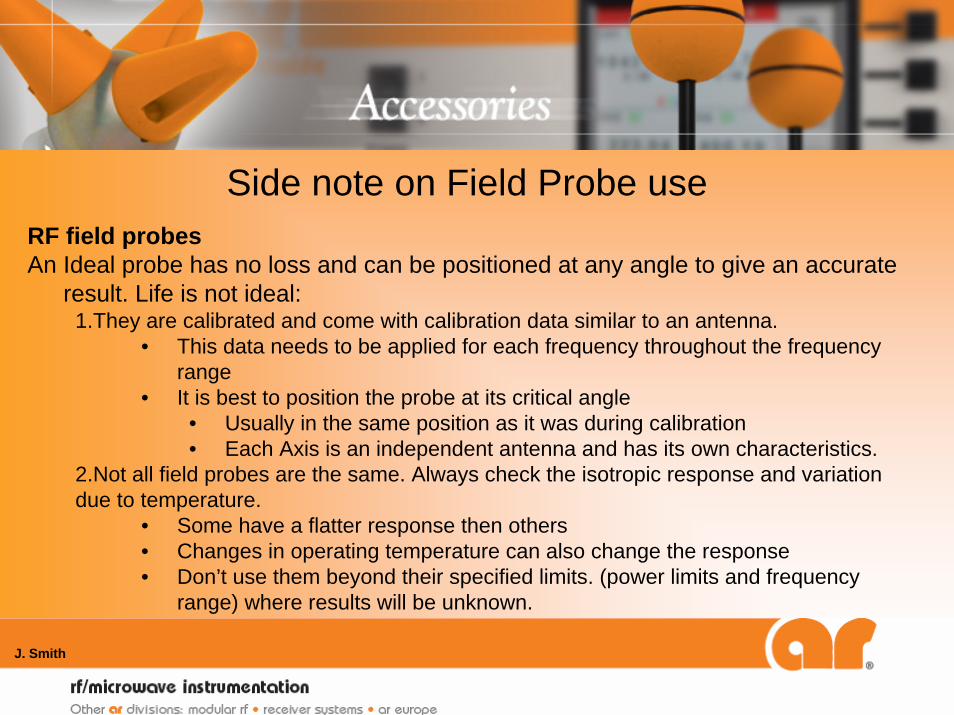
RF field probes An Ideal probe has no loss and can be positioned at any angle to give an accurate
result. Life is not ideal:1.They are calibrated and come with calibration data similar to an antenna.
• This data needs to be applied for each frequency throughout the frequency range
• It is best to position the probe at its critical angle • Usually in the same position as it was during calibration • Each Axis is an independent antenna and has its own characteristics.
2.Not all field probes are the same. Always check the isotropic response and variation due to temperature.
• Some have a flatter response then others• Changes in operating temperature can also change the response• Don’t use them beyond their specified limits. (power limits and frequency
range) where results will be unknown.

Uniform field calibrationPerformed at 1.8 times the desired field strength.
For testing at 10V/m the calibration is run at 18V/m
The reason of running a test at 1.8x the level is to verify the RF amplifier has the ability to reach the required field when the 80% 1KHz Amplitude Modulation is applied.
(Note:1.8 higher filed requires 3.24 times more amplifier power)
An EMC Lab performing testing at multiple levels 1V/m, 3V/m, 10V/m, 30V/m, and/or others, they need only to perform the calibration at 1.8x the max level they will test to and then they can scale the power down.
J. Smith
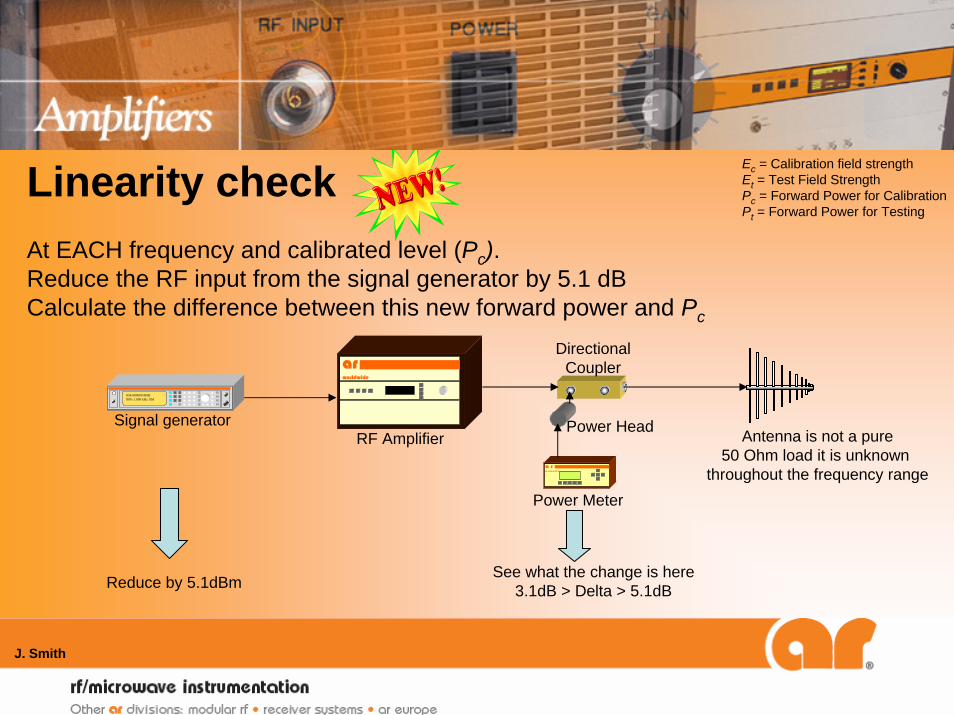
Linearity checkAt EACH frequency and calibrated level (Pc). Reduce the RF input from the signal generator by 5.1 dB Calculate the difference between this new forward power and Pc
Ec = Calibration field strengthEt = Test Field StrengthPc = Forward Power for CalibrationPt = Forward Power for Testing
J. Smith
854.000000 MHz 80% 1.000 kHz AM
Signal generator
ar worldwide
RF Amplifier a r w o r l d w i d e
Directional Coupler
Power Head
Power Meter
Reduce by 5.1dBm See what the change is here3.1dB > Delta > 5.1dB
Antenna is not a pure50 Ohm load it is unknown
throughout the frequency range

Linearity check
The difference needs to be between 3.1 and 5.1 dB If < 3.1 compression is too large. If > 5.1 the amplifier is in expansion and is nonlinear.
This may occur with Traveling Wave Tube Amplifiers (TWT), but is minor and should not be of concern.
This is called the 2dB compression point by the standard.
Ec = Calibration field strengthEt = Test Field StrengthPc = Forward Power for CalibrationPt = Forward Power for Testing
J. Smith

From the calibrated test data the test power (Pt) can be found.
For testing the intended field strength the forward test power is needed for each frequency:
5.1dB comes from: ⎟⎠⎞
⎜⎝⎛•=
tEER clog20)dB(
⎟⎠⎞
⎜⎝⎛•=1018log20)dB(R
1.5)dB( =R
Ec = Calibration field strengthEt = Test Field StrengthPc = Forward Power for CalibrationPt = Forward Power for Testing
dB1.5)dB( −=−= cct PRPP
J. Smith
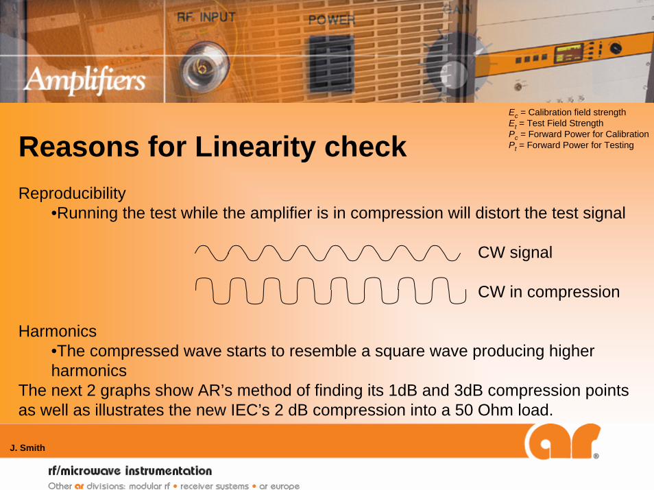
Reasons for Linearity checkReproducibility
•Running the test while the amplifier is in compression will distort the test signal
CW signal
CW in compression
Harmonics•The compressed wave starts to resemble a square wave producing higher harmonics
The next 2 graphs show AR’s method of finding its 1dB and 3dB compression points as well as illustrates the new IEC’s 2 dB compression into a 50 Ohm load.
Ec = Calibration field strengthEt = Test Field StrengthPc = Forward Power for CalibrationPt = Forward Power for Testing
J. Smith
Exa
mpl
e of
com
pres
sed
pow
er
J. Smith
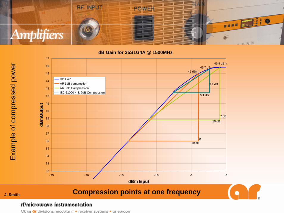
dB Gain for 25S1G4A @ 1500MHz
32
33
34
35
36
37
38
39
40
41
42
43
44
45
46
47
-25 -20 -15 -10 -5 0
dBm Input
dBm
Out
put
DB GainAR 1dB comprestionAR 3dB CompressionIEC 61000-4-3: 2dB Compression
45.7 dBm45 dBm
45.8 dBm
10 dB
10 dB9
7 dB
5.1 dB
3.1 dB
Compression points at one frequency

J. Smith
Exa
mpl
e of
com
pres
sed
pow
er
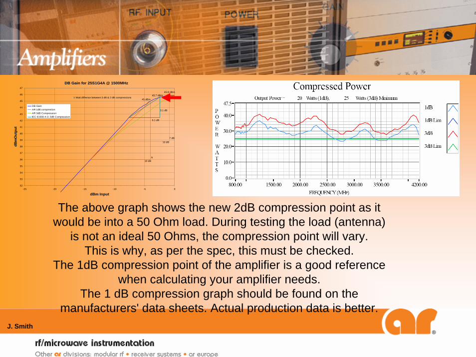
The above graph shows the new 2dB compression point as it would be into a 50 Ohm load. During testing the load (antenna)
is not an ideal 50 Ohms, the compression point will vary. This is why, as per the spec, this must be checked.
The 1dB compression point of the amplifier is a good reference when calculating your amplifier needs.
The 1 dB compression graph should be found on the manufacturers' data sheets. Actual production data is better.
J. Smith
DB Gain for 25S1G4A @ 1500MHz
32
33
34
35
36
37
38
39
40
41
42
43
44
45
46
47
-25 -20 -15 -10 -5 0
dBm Input
dBm
Out
put
DB GainAR 1dB comprestionAR 3dB CompressionIEC 61000-4-3: 2dB Compression
45.7 dBm45 dBm
45.8 dBm
10 dB
10 dB9
7 dB
5.1 dB
3.1 dB
1 Watt diffrence between 3 dB & 2 dB compressions

Window size is variable >1GHz (Annex H normative)
J. Smith
•For each window the antenna can then be moved around for optimal positioning for the calibration of that window•Each window will need to be calibrated separately.
•If 0.5m windows are used, 9 different calibrations will need to be run with 9 different antenna locations.
•When only 4 probe positions are used, as in this case, all probe positions must be used (cannot remove 25%)•Then for large EUTs filling the total area.
•The EUT will need to be tested 9 times on each side•Increased test time!
•Smaller EUTs only need be tested to illuminate the area of the EUT (in example to left only windows 1, 2, 5, and 6)•1 meter test distance
1.5m
1.5m
0.5mUniform field probe positions
9
123
4 5 6
78
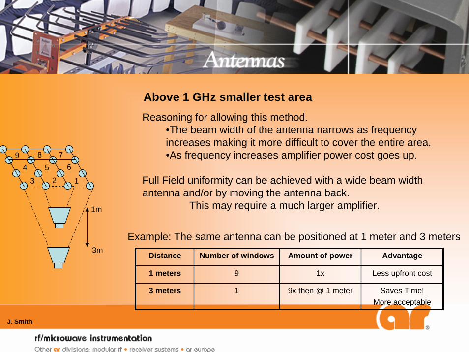
Above 1 GHz smaller test area
J. Smith
Reasoning for allowing this method.•The beam width of the antenna narrows as frequency increases making it more difficult to cover the entire area.•As frequency increases amplifier power cost goes up.
Full Field uniformity can be achieved with a wide beam width antenna and/or by moving the antenna back.
This may require a much larger amplifier.1m
3mDistance Number of windows Amount of power Advantage
1 meters 9 1x
9x then @ 1 meter
Less upfront cost
3 meters 1 Saves Time! More acceptable
Example: The same antenna can be positioned at 1 meter and 3 meters
9
123
4 5 678

J. Smith
⎥⎦⎤
⎢⎣⎡=Θ −
DW2
tan2 1
⎥⎦⎤
⎢⎣⎡Θ=
2tan2DW
( )2tan2 Θ=
WD
=Θ 3dB beam width of the antenna at specified frequency
=W Window width
=D Antenna distance
Using simple Geometry we can calculate window size or angle needed
28°
41°
74°
1.5 m
1 m
2 m
3 m
Antenna

Increased Frequency RangeThe standard does not dictate that the same level needs to be
applied over the whole frequency range. •This is left to the product standards
80 to 1000 MHz will most likely be one level, same as before.
800 to 960 MHz and 1.4 to 6 GHz Was added for Radio Phones (Cell Phone) and other emitters. So depending on the device and/or location the product is sold
in or used in, the frequency range/s and level/s may vary.This will be determined by future Product Standards
J. Smith

Increased Frequency RangeReasons for increase
Annex G of the standard lists approved frequency allocations used for the basis of the new 6 GHz frequency expansion.
With the explosion of wireless communication for voice and data transfer there is a definite need for product rigidness to
withstand today and tomorrow’s threats.
Product standards will be updated in the future But:
Higher frequency test needs to be incorporated to protect the products from these new threats now!
J. Smith
J. Smith
Increased Frequency RangeReasons for testing beyond the requirements
It is more than meeting the specs and Law, it is about product quality and reliability
The standard is written to cover common Electromagnetic influences that are present at release.
With other influences out there, it is important to catch potential issues up front prior to product release.
It could cost $millions$ if failures occur at the consumer level.
Example: Emergency communication head sets
cable TV boxes, ANSI specification is being created to test to 100V/m
Customer satisfaction is very important for product longevity and company growth
J. Smith
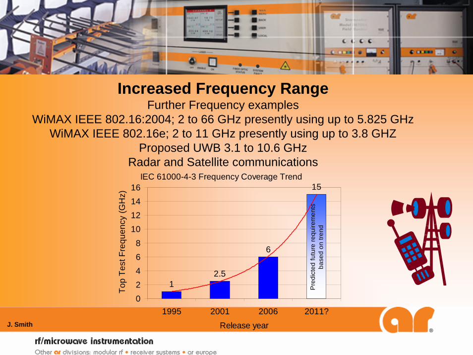
Increased Frequency RangeFurther Frequency examples
WiMAX IEEE 802.16:2004; 2 to 66 GHz presently using up to 5.825 GHzWiMAX IEEE 802.16e; 2 to 11 GHz presently using up to 3.8 GHZ
Proposed UWB 3.1 to 10.6 GHzRadar and Satellite communications
IEC 61000-4-3 Frequency Coverage Trend
12.5
6
15
02468
10121416
1995 2001 2006 2011?Release year
Top
Test
Fre
quen
cy (G
Hz)
Pre
dict
ed fu
ture
requ
irem
ents
ba
sed
on tr
end
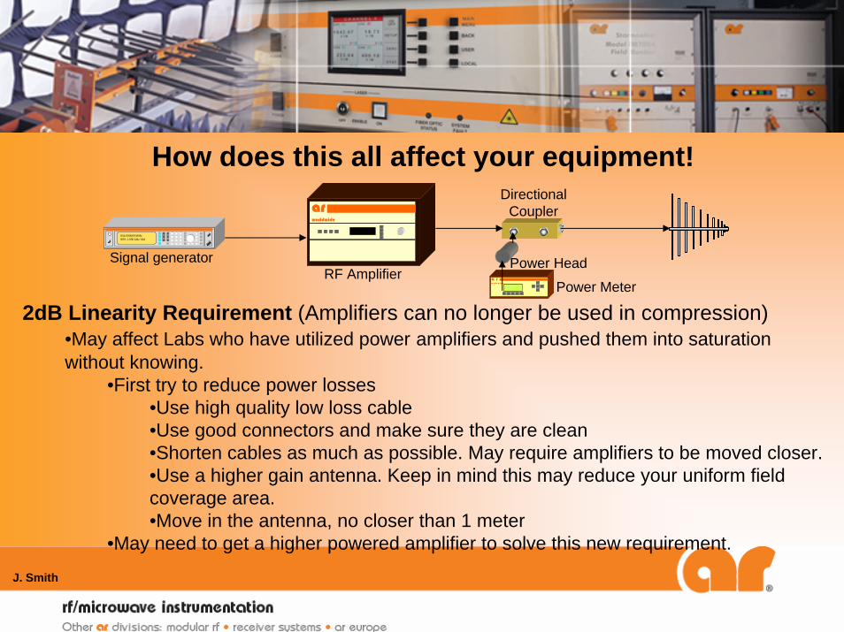
How does this all affect your equipment!
2dB Linearity Requirement (Amplifiers can no longer be used in compression)•May affect Labs who have utilized power amplifiers and pushed them into saturation without knowing.
•First try to reduce power losses•Use high quality low loss cable•Use good connectors and make sure they are clean•Shorten cables as much as possible. May require amplifiers to be moved closer.•Use a higher gain antenna. Keep in mind this may reduce your uniform field coverage area.•Move in the antenna, no closer than 1 meter
•May need to get a higher powered amplifier to solve this new requirement.
J. Smith
854.000000 MHz 80% 1.000 kHz AM
Signal generator
ar worldwide
RF Amplifier a r w o r l d w i d e
Directional Coupler
Power Head
Power Meter

How does this affect equipment!6dB Harmonics requirement
•TWT amplifiers which can be used for above 1 GHz will need to have filters to reduce the harmonic content
•Filters will have losses and reduce the output of the TWTA.•TWTs are not as linear throughout the range as the solid-state amplifiers are.
•Solid state amplifiers should not need filters.
J. Smith
25S1G4A 20T4G18A

How does this all affect your equipment!
Higher frequency requirements up to 6 GHz.•May require new Amplifiers and Antennas
•Use manufacturers data to help with linearity (1dB compression) and harmonic content•If harmonics are an issue (as in TWTA) check to see if filters are available
J. Smith
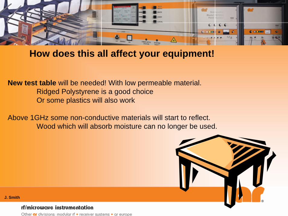
How does this all affect your equipment!
New test table will be needed! With low permeable material.Ridged Polystyrene is a good choiceOr some plastics will also work
Above 1GHz some non-conductive materials will start to reflect.Wood which will absorb moisture can no longer be used.
J. Smith

Selecting the correct equipment overview1. Select an antenna to use.
• Frequency range• Power handling• Beam width & gain
J. Smith
3. Select the correct amplifier• Use calculated power to select the correct amplifier
• Needs to be selected at the 1dB compression point
2. Calculate power requirements• Antenna data: based on measured data or gain• Calculate out all loses between amplifier and antenna
• Cables, directional coupler and connectors• Intended test distance (1 to 3 meters)
∗+−+=≤≅

J. Smith
Selecting the correct antennas
1. Select antennas to use.• This is the most important part of the process. Not all antennas are the same.
Just because you own an antenna doesn't mean it should be used for every application. Research your options. A one antenna solution can work but will be very costly in amplifier power requirements.
• 80 MHz – 1 GHz log-periodic is the best choice. • Combination antennas (biconical/log) that cover lower frequencies are
not always the best choice.• Above 1GHz log-periodic and horn antennas can be used.
• Horn antennas will direct the energy forward with more efficiency

J. Smith
Selecting the correct antenna• Above 1GHz ask the following questions:
• What size EUT will you be testing?• Is calibrating and testing multiple “windows” acceptable?• What test distance is acceptable?
• The ideal solution would be one antenna 80MHz – 6GHz with enough beam width to meet 1.5m X 1.5m window throughout the frequency range. (This is not presently available to my knowledge)
1.5m
1.5m
0.5mUniform field probe positions
9
123
4 5 6
78
⎥⎦⎤
⎢⎣⎡=Θ −
DW2
tan2 1
⎥⎦⎤
⎢⎣⎡Θ=
2tan2DW
( )2tan2 Θ=
WD
=Θ 3dB beam width of the antenna at specified frequency
=Θ 3dB beam width of the antenna at specified frequency
=W Window width=W Window width
=D Antenna distance=D Antenna distance
28°
41°
74°
1.5 m
1 m
2 m
3 m
Antenna
28°
41°
74°
1.5 m
1 m
2 m
3 m
Antenna

J. Smith
Selecting the correct antenna
• Select an antenna based on beam width, and power handling• Use antenna data provided by the antenna manufacturer
• Antenna Gain Graph• Antenna Factor Graph• Antenna input power vs. field Graph
• Note how manufacturer’s data was taken• Calculated or Actual measurement (free field, or chamber)
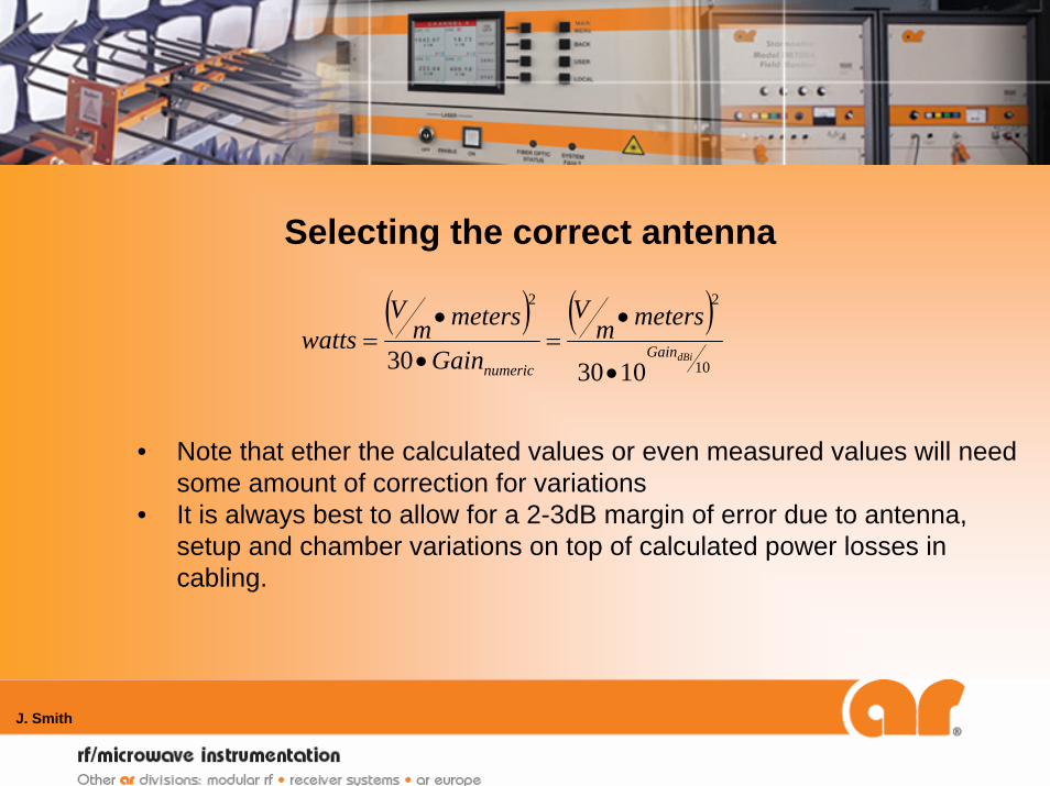
• Important Equations for calculating the required power once an antenna is selected ( ) ( )
10
22
103030 dBiGainnumeric
metersmV
Gain
metersmV
watts•
•=
•
•=
79.29)log(20 −−= torAntennaFacMHzGaindBi
J. Smith
( ) ( )10
22
103030 dBiGainnumeric
metersmV
Gain
metersmV
watts•
•=
•
•=
Selecting the correct antenna
• Note that ether the calculated values or even measured values will need some amount of correction for variations
• It is always best to allow for a 2-3dB margin of error due to antenna, setup and chamber variations on top of calculated power losses in cabling.

J. Smith
( ) ( )10
22
103030 dBiGainnumeric
metersmV
Gain
metersmV
watts•
•=
•
•=
Selecting the correct antenna
Example:• 10V/m field with 80% modulation applied
• Equivalent to 18V/m• 3 meter test distance • Using a double ridge antenna (using provided gain)
• Worst case gain is at 1GHz ~5.5dBi
( ) wattsmetersmVwatts dBi 39.271030
3/1810
5.5
2
=•
•=
J. Smith
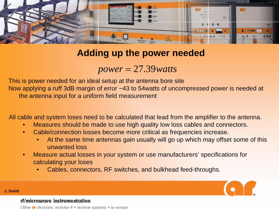
wattspower 39.27=
Adding up the power needed
This is power needed for an ideal setup at the antenna bore siteNow applying a ruff 3dB margin of error ~43 to 54watts of uncompressed power is needed at
the antenna input for a uniform field measurement
All cable and system loses need to be calculated that lead from the amplifier to the antenna. • Measures should be made to use high quality low loss cables and connectors. • Cable/connection losses become more critical as frequencies increase.
• At the same time antennas gain usually will go up which may offset some of this unwanted loss
• Measure actual losses in your system or use manufacturers’ specifications for calculating your loses
• Cables, connectors, RF switches, and bulkhead feed-throughs.
J. Smith
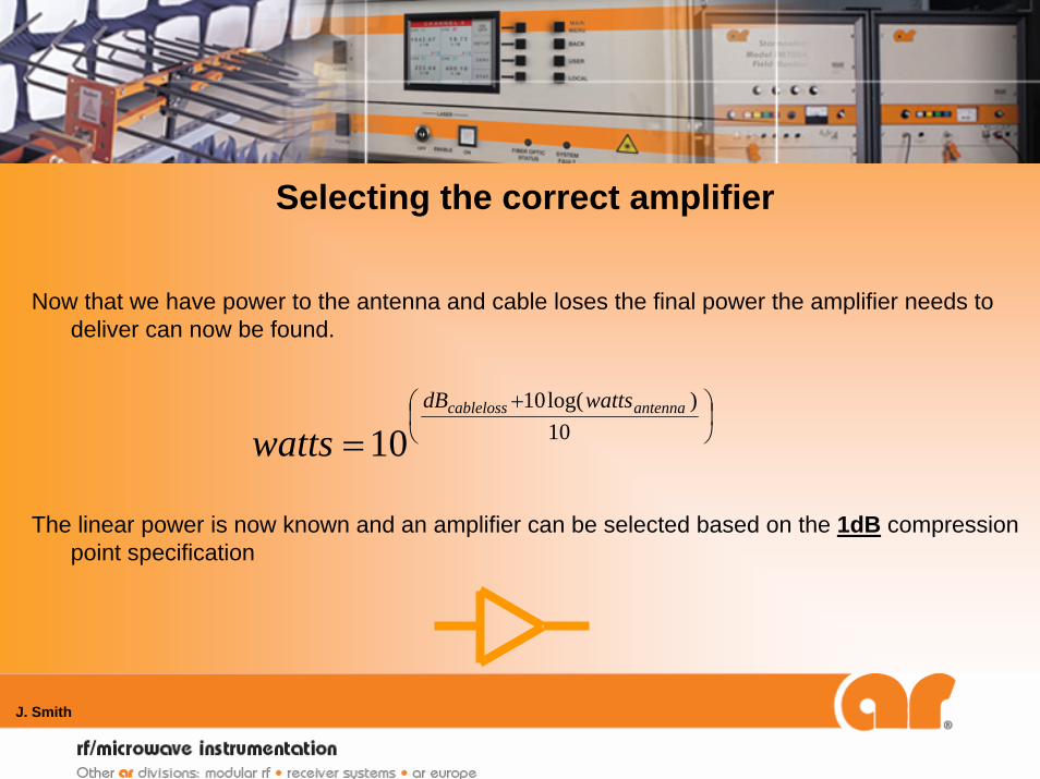
Selecting the correct amplifier
Now that we have power to the antenna and cable loses the final power the amplifier needs to deliver can now be found.
The linear power is now known and an amplifier can be selected based on the 1dB compression point specification
⎟⎠⎞
⎜⎝⎛ +
= 10)log(10
10antennacableloss wattsdB
watts
J. Smith
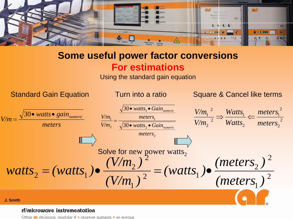
Some useful power factor conversionsFor estimations
Using the standard gain equation
metersgainwatts
V/m numeric••=
30
2
2
1
1
2
1
30
30
metersGainwatts
metersGainwatts
V/mV/m
numeric
numeric
••
••
= 22
21
2
12
2
21
metersmeters
WattsWatts
V/mV/m
⇐⇒
21
22
121
22
12 )(meters)(meters)(watts
)(V/m)(V/m)(wattswatts •=•=
Standard Gain Equation Turn into a ratio Square & Cancel like terms
Solve for new power watts2
J. Smith
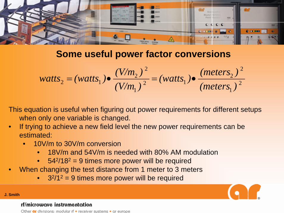
Some useful power factor conversions
This equation is useful when figuring out power requirements for different setups when only one variable is changed.
• If trying to achieve a new field level the new power requirements can be estimated:• 10V/m to 30V/m conversion
• 18V/m and 54V/m is needed with 80% AM modulation• 542/182 = 9 times more power will be required
• When changing the test distance from 1 meter to 3 meters• 32/12 = 9 times more power will be required
21
22
121
22
12 )(meters)(meters)(watts
)(V/m)(V/m)(wattswatts •=•=
J. Smith
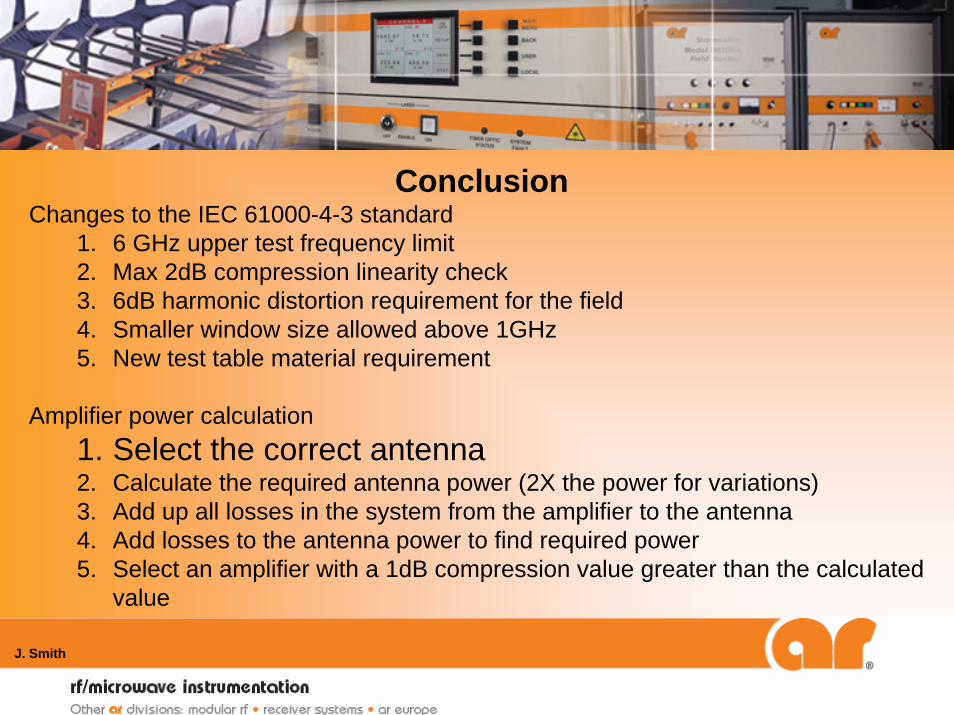
ConclusionChanges to the IEC 61000-4-3 standard
1. 6 GHz upper test frequency limit2. Max 2dB compression linearity check3. 6dB harmonic distortion requirement for the field4. Smaller window size allowed above 1GHz5. New test table material requirement
Amplifier power calculation1. Select the correct antenna2. Calculate the required antenna power (2X the power for variations)3. Add up all losses in the system from the amplifier to the antenna4. Add losses to the antenna power to find required power5. Select an amplifier with a 1dB compression value greater than the calculated
value

J. Smith
Any questions?
Thank you for your attention!!!
Jason H. SmithSupervisor Applications Engineerar rf/microwave instrumentation
160 School House Road Souderton, PA 18964-9990 [email protected]