idiosyncratic sectoral growth, balanced growth, and ... · sectors), dupor found that aggregate...

Economic Quarterly– Volume 104, Number 2– Second Quarter 2018– Pages 79—101

Idiosyncratic SectoralGrowth, Balanced Growth,and Sectoral Linkages

Andrew Foerster, Eric LaRose, and Pierre-Daniel Sarte

In general, there is substantial heterogeneity in value added, grossoutput, and production patterns across sectors within the US econ-omy. There is also considerable asymmetry in intermediate goods

linkages; that is, some sectors are much larger suppliers of intermediategoods to different sectors, on average, than others. Such heterogeneitysuggests that there may be significant differences in the extent to whichshocks to individual sectors not only affect aggregate output, but alsotransmit to other sectors.1

In this paper, in contrast to previous literature focusing on shorter-run variations in economic activity, we explore how longer-run growthin different sectors affects other sectors and overall aggregate growth.We consider a neoclassical multisector growth model with sector-specificcapital and linkages between sectors in intermediate goods. In partic-ular, we investigate the properties of a balanced growth path wheretotal factor productivity (TFP) growth is sector-specific. We derive arelatively simple formula that simultaneously captures all relationshipsbetween value-added growth and TFP growth across sectors. We thenstudy the effect of changes in TFP growth in one sector on value-addedgrowth in every other sector. In addition, we can use the Divisia indexfor aggregate value-added growth to calculate the effect of a change inTFP growth in a given sector on aggregate GDP growth. Finally, using

The views expressed herein are those of the authors and do not necessarily reflectthose of the Federal Reserve Bank of Richmond, the Federal Reserve Bank of SanFrancisco, or the Federal Reserve System. We thank Caroline Davis, Toan Phan,Santiago Pinto, and John Weinberg for helpful comments.

1 See, for instance, Acemoglu, Carvalho, Ozdaglar, and Tahbaz-Salehi (2012); Foer-ster, Sarte, and Watson (2011); Atalay (2017); and Miranda-Pinto (2018).

DOI: https://doi.org/10.21144/eq1040202

80 Federal Reserve Bank of Richmond Economic Quarterly

data on value-added growth for each sector over the period 1948-2014,we recover each sector’s model-implied mean TFP growth over this pe-riod and examine how sectoral changes in TFP growth in practice carryover to other sectors.

In all three of the above exercises, we also consider a special case ofour model without capital. This case collapses to the model consideredby Hulten (1978), or Acemoglu et al. (2012). In that model, absentcapital, the impact of a level change in sectoral TFP on GDP is entirelycaptured by that sector’s share in GDP.2 We show that a version ofthis result also holds in growth rates along the balanced growth path.In that special case, other microeconomic details of the environmentbecome irrelevant as long as we can observe the distribution of value-added shares across sectors.

More generally, in the benchmark model, value-added growth andthe effects of changes in TFP growth in a given sector on GDP growthdepend on that sector’s capital intensity, its share of value added ingross output, and the degree to which its goods are used as interme-diates by other sectors. In this regard, in a multisector model withcapital, it becomes important to have information pertaining to theunderlying microeconomic structure of the economy beyond what iscaptured in shares. Fortunately, the model delivers a simple expressionof relevant parameters that can easily be constructed from sectoral-leveldata provided by government agencies.

Using such data, we can quantify the effects of changes in sectoralTFP growth and compare these results to the special case of our modelwhere a version of Hulten (1978) holds in growth rates. In the sevensectors we consider in this paper, sectors vary widely in their sharesof capital in value added and value added in total output, and somesectors are considerably more important suppliers of intermediate goodsthan others. Overall, we find that adding capital to the model createssubstantial spillovers across sectors resulting from TFP growth changesthat, for every sector, substantially increase the responsiveness of GDPgrowth to such changes. These spillover effects are larger for sectorsmore integral to sectoral linkages in intermediates, a finding consistentwith the literature we discuss below.

2 Pasten, Schoenle, and Weber (2018) and Baqaee and Farhi (2018) show that, evenin a model without capital, this result may not hold due to factors such as heterogeneousprice rigidity and nonlinearities in production.

Foerster, LaRose, Sarte: Growth and Sectoral Linkages 81

1. RELATED LITERATURE

The modern literature on multisector growth models started with thereal business cycle model presented in Long and Plosser (1983). Intheir model, a representative agent chooses labor inputs and commod-ity inputs to n sectors, with linkages between sectors in inputs anduncorrelated exogenous shocks to each sector. Taking the model tothe data with six sectors, they found substantial comovement in out-put across sectors; furthermore, shocks to individual sectors generallyled to large aggregate fluctuations, particularly for sectors that heavilyserved as inputs in production.

For many years, there existed a sense that at more disaggregatedlevels than that of Long and Plosser (1983), idiosyncratic sectoralshocks should fail to affect aggregate volatility. Lucas (1981), in par-ticular, argued that in an economy with disaggregated sectors, manysector-specific shocks would occur within a given period and roughlycancel each other out in a way consistent with the Law of Large Num-bers. Dupor (1999) helped formalize the conditions under which theintuition in Lucas (1981) would apply. He considered an n-sector econ-omy with linkages between firms in intermediates as well as full depreci-ation of capital. Assuming all sectors sold nonzero amounts to all othersectors, and that every row total in the matrix of linkages was the same(i.e., every sector is equally important as an input supplier to all othersectors), Dupor found that aggregate volatility converged toward zeroat a rate of

√n; the underlying structure of the input-output matrix

was irrelevant as long as it satisfied those conditions.Horvath (1998) countered that Dupor’s irrelevance theorem failed

to hold because, in practice, sectors are not uniformly important asinput suppliers to other sectors. He observed that at high levels ofdisaggregation in US data, the matrix of input-output linkages becamequite sparse, with only a few sectors selling widely to others; conse-quently, sectoral shocks could explain a significant share of aggregatevolatility, which would decline at a rate much slower than

√n. (Horvath

[2000] showed that his earlier result still held in more general models in-cluding, among other things, linkages between sectors in investments.)Acemoglu et al. (2012) expand on Horvath’s idea by analyzing thenetwork structure of linkages and conclude that it is the asymmetry,rather than the sparseness, of input-output linkages that determinesthe decay rate of aggregate volatility. In a multisector model with link-ages between sectors in investment as well as intermediates, Foerster,Sarte, and Watson (2011) find evidence of a high level of asymmetryin the data, consistent with Acemoglu et al. (2012). They also showthat, starting with the Great Moderation around 1983, roughly halfthe variation in aggregate output stems from sectoral shocks.


As an additional perspective on the failure of sectoral shocks toaverage out, Gabaix (2011) also points out that the “averaging out”argument will not hold when the distribution of firms (or sectors) isfat-tailed, meaning a few large firms (or sectors) dominate the economy.In such a case, aggregate volatility decays at rate 1

lnn , and idiosyncraticmovements can cause large variations in output growth.

While it should be clear from this section that the literature on mul-tisector growth models has mostly focused on the relationship betweenaggregate and sectoral volatility, this paper focuses instead on the re-lationship between aggregate and sectoral growth. The arguments ofHorvath (1998), Acemoglu et al. (2012), and others regarding the na-ture of input-output linkages still hold relevance for sectoral growth.In that vein, the analysis herein builds more directly on the work ofNgai and Pissarides (2007). In that paper, the authors focus on theeffects of different TFP growth rates across sectors on sectoral employ-ment shares. The model we present extends their work by explicitlycapturing all pairwise linkages in intermediate goods in the economywhile additionally allowing every sector to produce capital.

2. ECONOMIC ENVIRONMENT

We consider an economy with n sectors. For simplicity, we assume thatutility is linear in the final consumption good. Preferences are givenby

E0

∞∑t=0

βtCt

Ct =n∏j=1

(cj,tθj

)θj,

n∑j=1

θj = 1,

where Ct represents an aggregate consumption bundle taken to be thenumeraire good.

Gross output in a sector j results from combining value added andmaterials output according to

yj,t =

(vj,tγj

)γj ( mj,t

1− γj

)1−γj,

where yj,t, vj,t, and mj,t denote gross output, value added, and materi-als output, respectively, used by sector j at time t. Materials output ina given sector j results from combining different intermediate materials


from all other sectors, as described by the production function,

mj,t =n∏i=1

(mij,t

φij

)φij,

n∑i=1

φij = 1,

where mij,t denotes the use of materials produced in sector i by sectorj at time t.

Value added in sector j is produced using capital and labor,

vj,t = zj,t

(kj,tαj

)αj ( `j,t1− αj

)1−αj,

where zj,t denotes a technical shift parameter that scales production ofvalue added, which we refer to as value-added TFP.

Capital is sector-specific, so that output from only sector j can beused to produce capital for sector j, and it accumulates according tothe law of motion,

kj,t+1 = xj,t + (1− δ) kj,t,

where xj,t represents investment in sector j at time t and δ denotes thedepreciation rate of capital.

Goods market clearing requires that

cj,t +n∑i=1

mji,t + xj,t = yj,t,

while labor market clearing requires thatn∑j=1

`j,t = 1.

Here, we assume that aggregate labor supply is inelastic and set toone. We also assume that labor can move freely across sectors so thatworkers earn the same wage, wt, in all sectors.

Finally, we assume that TFP growth in sector j, ∆ ln zj,t, followsan AR(1) process,

∆ ln zj,t = (1− ρ) gj + ρ∆ ln zj,t−1 + ηj,t,

where ρ < 1 and ηj,t ∼ D with mean zero for each j.

3. PLANNER’S PROBLEM

The economy we have just described presents no frictions, so thatdecentralized allocations in the competitive equilibrium are optimal.Thus, we derive these allocations by solving the following planner’s


problem:

max L =∞∑t=0

βtn∏j=1

(cj,tθj

)θj(1)

such that ∀ j and t,

cj,t +n∑i=1

mji,t + xj,t =

(vj,tγj

)γj ( mj,t

1− γj

)1−γj, (2)

mj,t =n∏i=1

(mij,t

φij

)φij, (3)

vj,t = zj,t

(kj,tαj

)αj ( `j,t1− αj

)1−αj, (4)

kj,t+1 = xj,t + (1− δ) kj,t, (5)

and ∀ t,n∑j=1

`j,t = 1. (6)

Let pyj,t, pvj,t, p

mj,t, and pxj,t denote the Lagrange multipliers asso-

ciated with, respectively, the resource constraint (2), the productionof value added (4), the production of materials (3), and the capitalaccumulation equation (5) in sector j at date t.

The first-order conditions for optimality yield

θjCtcj,t

= pyj,t.

This expression also defines an ideal price index,

1 =n∏j=1

(pyj,t

)θj. (7)

We additionally have that

pvj,tvj,t = γjpyj,tyj,t.

Likewise,

pmj,tmj,t =(1− γj

)pyj,tyj,t.

The above two expressions define a price index for gross output,

pyj,t =(pvj,t)γj (pmj,t)1−γj .


In addition, we have that

pyi,tmij,t = φijpmj,tmj,t,

which gives material prices in terms of gross output prices,

pmj,t =n∏i=1

(pyi,t

)φij,

and

wt`j,t = (1− αj)pvj,tvj,t,where wt is the Lagrange multiplier associated with the labor marketclearing condition (6).

From the law of motion for capital accumulation, we have that

pxj,t = pyj,t.

Finally, the Euler equation associated with optimal investment dictates

pxj,t = βEt

[αjpvj,t+1vj,t+1

kj,t+1+ pxj,t+1 (1− δ)

].

The first-order conditions give rise to natural expressions of themodel parameters as shares that are readily available in the data. Inparticular, θj represents the share of sector j in nominal consump-tion, and γj represents the share of value added in total output insector j, while φij represents materials purchased from sector i by sec-tor j as a share of total materials purchased in sector j. Furthermore,1 − αj equals the share of total wages in nominal value added in sec-tor j, and consequently, αj represents capital’s share in nominal valueadded. Nominal value added in sector j in this economy is then givenby pvj,tvj,t = γip

yj,tyj,t, and it follows that GDPt =

∑j p

vj,tvj,t.

In the remainder of this paper, we adopt the following notation:Γd = diag{γj}, αd = diag{αj}, Θ = (θ1, ..., θn), and Φ = {φij}.

Some Benchmark Results in Levels

A special case of the economic environment presented above is onewhere αj = 0 ∀j, which, absent any growth in sectoral TFP or shocks,reduces to the static economies of Hulten (1978) or Acemoglu et al.(2012). In this case, aggregate value added, or GDP, is given by theconsumption bundle Ct and

∂ lnGDPt∂ ln zj,t

= svj ∀t,

where svj is sector j’s value-added share in GDP, and we summarizethese shares in a vector, sv = (sv1, ..., s

vn), given by

sv = Θ(I − (I − Γd)Φ′)−1Γd. (8)


As shown in Hulten (1978), in this special case, a sector’s value-addedshare entirely captures the effect of a level change in TFP on GDP.Accordingly, Acemoglu et al. (2012) refer to the object Θ(I − (I −Γd)Φ

′)−1Γd as the influence vector.A model with capital is dynamic but, in the long run, converges

to a steady state in levels absent any sectoral TFP growth. With adiscount factor β close to 1, the effect of a level change in sectoral logTFP on log GDP continues to be given primarily by sectoral shares,as in equation (8). In other words, Hulten’s (1978) result continues tohold in an economy with capital in that the variation in the effects ofsectoral TFP changes on GDP is determined by the variation in sectoralshares. In this case, however, sectoral shares need to be adjusted by afactor that is constant across sectors and approximately equal to theinverse of the mean employment share.

With exogenous sectoral TFP growth, the economy no longer achievesa steady state in levels. Instead, with constant sectoral TFP growth,the steady state of the economy may be defined in terms of sectoralgrowth rates along a balanced growth path. Along this path, the ef-fects of TFP growth changes on GDP growth involve additional con-siderations. In particular, sectoral linkages in intermediates mean thatchanges in sectoral TFP growth in one sector potentially affect value-added growth rates in every other sector and, therefore, can impactoverall GDP growth beyond changes in shares. These sectoral linkagesconsequently create a multiplier effect that, as we show below, can leadto a total impact of a TFP growth change in a given sector that isseveral times larger than that sector’s share in GDP.

4. SOLVING FOR BALANCED GROWTH

We now allow for each sector to grow at a different rate along a balancedgrowth path. In particular, we derive and explore the relationships thatlink different sectoral growth rates to each other and study how TFPgrowth rates in one sector affect all other sectors and the aggregatebalanced growth path.

Consider the case where zj,t is growing at a constant rate along anonstochastic steady-state path, that is ηj,t = 0 and ∆ ln zj,t = gj ∀j,t. Moreover, the resource constraint (2) in each sector requires thatall variables in that equation grow at the same constant rate along abalanced growth path. Therefore, we normalize the model’s variablesin each sector by a sector-specific factor µj,t. In particular, we defineyj,t = yj,t/µj,t, cj,t = cj,t/µj,t, mji,t = mji,t/µj,t, and xj,t = xj,t/µj,t. Weshow that detrending the economy yields a system of equations that isstationary in the normalized variables along the balanced growth path


and where the vector µt = (µ1,t, ..., µn,t)′ can be expressed as a function

of the underlying parameters of the model only.

Detrending the Economy

The capital accumulation equation in sector j can be written underthis normalization as

kj,t+1 = xj,tµj,t + (1− δ) kj,t,so that

kj,t+1 = xj,t + (1− δ) kj,t(µj,t−1

µj,t

),

where kj,t = kj,t/µj,t−1.Using this last equation, we can write value added in sector j as

vj,t = zj,t

(kj,tµj,t−1

αj

)αj (`j,t

1− αj

)1−αj.

The aggregate labor constraint in each period,∑

j `j,t = 1, implies that

the labor shares, `j,t, are already normalized: ˜j,t = `j,t. Then defining

vj,t = vj,t/(zj,t(µj,t−1

)αj), the expression for value added becomesvj,t =

(kj,tαj

)αj (`j,t

1− αj

)1−αj.

The equation for materials used in sector j can be written in nor-malized terms as

mj,t =

n∏i=1

(mij,t

φij

)φij,

where mj,t = mj,t/∏ni=1 µ

φiji,t . It follows that gross output in sector j

becomes, in normalized terms,

yj,tµj,t =

(vj,tzj,tµ

αjj,t

γj

)γj mj,t∏ni=1 µ

φiji,t

1− γj

1−γj

,

which may be rewritten as

yj,t =

(vj,tγj

)γj ( mj,t

1− γj

)1−γj[zγjj,tµ

γjαjj,t−1

µj,t

n∏i=1

µ(1−γj)φiji,t

]. (9)

Observe that for the detrended variables to be constant along abalanced growth path, it must be the case that the expression in square


brackets is also constant along that path. Thus, we can use equation(9) to solve for µj,t as a function of the model parameters. In particular,we can rewrite the term in square brackets as

zγjj,tµ

γjαjj,t−1µ

γjαj−1

j,t

µγjαjj,t

n∏i=1

µ(1−γj)φiji,t ,

where we aim for the growth rate of µj,t to be constant. Thus, withoutloss of generality, we choose µj,t such that

zγjj,tµ

γjαj−1

j,t

n∏i=1

µ(1−γj)φiji,t = 1,

which in logs gives

γj ln zj,t +(γjαj − 1

)lnuj,t +

n∑i=1

(1− γj

)φij lnµi,t = 0. (10)

In matrix form, with zt = (z1,t, ..., zn,t)′, equation (10) becomes

Γd ln zt + (Γdαd − I) lnµt + (I − Γd) Φ′ lnµt = 0.

It follows that along a balanced growth path,

∆ lnµt =(I − Γdαd − (I − Γd) Φ′

)−1Γdgz, (11)

where gz = (g1, ..., gn)′.

Sectoral Value Added and GDP along aBalanced Growth Path

Having derived expressions in terms of the normalizing factors for µj,t,we now derive the normalizing factors for value added in each sector.By construction, these factors in turn will grow at the same rate asvalue added in each sector. As given above, the normalizing factor forvalue added in sector j, denoted as µvj,t, is zj,tµ

αjj,t−1. In vector form,

this becomes

∆ lnµvt = ∆ ln zt + αd(I − Γdαd − (I − Γd) Φ′

)−1Γd∆ ln zt−1,

so that along a balanced growth path,

∆ lnµvt =[I + αd

(I − Γdαd − (I − Γd) Φ′

)−1Γd

]gz. (12)

In other words, in this economy, TFP growth in each sector potentiallyaffects value-added growth in every other sector through a matrix thatsummarizes all linkages in the economy,[I + αd (I − Γdαd − (I − Γd) Φ′)−1 Γd

].Moreover, these effects may be


summarized analytically by

∂∆ lnµvt∂gz

=[I + αd

(I − Γdαd − (I − Γd) Φ′

)−1Γd

], (13)

where the element in row i and column j of this matrix represents theeffect of an increase in TFP growth in sector j on value-added growthrates in sector i:

∂∆ lnµvi,t∂gj

= 1 + αiγjξij if i = j,

where (I − Γdαd − (I − Γd) Φ′)−1 = {ξij}, or∂∆ lnµvi,t∂gj

= αiγjξij if i 6= j.

As mentioned above, growth rates in every sector depend on TFPgrowth rates in every sector because of the linkages between sectorsin intermediate goods. The matrix (I − Γdαd − (I − Γd) Φ′)−1 Γd sug-gests that, all else equal, TFP growth changes in sectors that are morecapital intensive (i.e., where αj is higher) and have higher shares ofvalue added in gross output (i.e., where γj is higher) will tend to havelarger effects on other sectors. Additionally, more capital-intensive sec-tors will tend to have larger responses to TFP growth changes in othersectors.

The expression for GDP gives us

GDPt =n∑j=1

pvj,tvj,t.

Using a standard Divisia index, we can express aggregate GDP growthas a weighted average of sectoral growth rates in real value added,

∆ lnGDPt =n∑j=1

svj,t∆ ln vj,t, (14)

where svj,t is the share of sector j in nominal value added,3

svj,t =pvj,tvj,t∑nj=1 p

vj,tvj,t

.

Define ∆ ln vt = ∆ lnµvt along the balanced growth path. We maythen substitute our expression for lnµvt in terms of TFP to obtain the

3 These shares also hold in normalized form, so that svj,t =pvj,tvj,t∑nj=1 p

vj,tvj,t

, and are

constant along the balanced growth path. Here we take the shares as exogenous pa-rameters given in the data, but they can alternatively be solved as part of the steadystate in normalized variables.


balanced growth rate of real aggregate GDP in terms of TFP growth:

∆ lnGDPt = sv[I + αd

(I − Γdαd − (I − Γd) Φ′

)−1Γd

]gz.

This last expression implies that, with constant shares,

∂∆ lnGDPt∂gz

= sv[I + αd

(I − Γdαd − (I − Γd) Φ′

)−1Γd

], (15)

with the effect of a change in TFP growth in sector j on GDP growththen given by the jth element,

∂∆ lnGDPt∂gj

=

(svj +

n∑i=1

sviαiγjξij

).

The above equation shows that TFP changes in sectors with highershares of value added in gross output, and whose intermediates aremore heavily used by other sectors, will have larger effects on changesin GDP growth.

Balanced Growth with No Capital

Consider the special case of our model with no capital accumulation,αj = 0 ∀j. Then the formula for value added in sector j becomes

vj,t = zj,t`j,t.

Since labor supply, `j,t, is already normalized as implied by the laborsupply constraint, the normalizing factor for value added in sector j attime t, µvj,t, is simply µ

vj,t = zj,t, so that along a balanced growth path

∆ lnµvt = gz. Then we have

∂∆ lnµvt∂gz

= I, (16)

so a change in TFP growth in sector j changes value-added growth insector j by the same amount and has no impact on value-added growthin other sectors, even though sector j is linked to other sectors throughintermediate goods. From equation (16), in the model without capital,we then have along a balanced growth path

∂∆ lnGDPt∂gz

= sv, (17)

which has jth element svj . Put another way, a change in TFP growthin sector j increases the growth rate of real aggregate GDP by thatsector’s share of value added in GDP. To a first order, the intermediategoods matrix Φ and other details are irrelevant as long as we know thevalue-added distribution of sectors.


In the rest of this paper, we match this model to the data with n = 7sectors in order to quantify equations (13) and (15), and we also invert[I + αd (I − Γdαd − (I − Γd) Φ′)−1 Γd

]in equation (11) to obtain the

implied TFP growth rates in each sector. We also use equations (16)and (17) to compare our quantitative benchmark results to those in thecase without capital.

5. DATA

As described above, the natural expressions of several model parame-ters as shares make it easy to match this model to available data. Allof the model parameters, consisting of the Φ matrix, the γj’s, and theαj’s, can be obtained through the Bureau of Economic Analysis (BEA),which provides data at various levels of industry aggregation going backto 1947.

The highest level of aggregation reported by the BEA is the fifteen-industry level. We drop one industry corresponding to Government,and then we consolidate the fourteen remaining industries into sevenbroader sectors: Agriculture, Forestry, Fishing, and Hunting; Min-ing and Utilities; Construction; Manufacturing; Wholesale and RetailTrade; Transportation and Warehousing; and Services. The seven-sector level is a high enough level of aggregation to give us a broadoverview of the economy, and these constructed sectors closely matchthe six sectors examined by Long and Plosser (1983).

To assemble the Φ matrix for our benchmark year, 2014, we rely ondata from the BEA’s Make-Use Tables, which at the fifteen-industrylevel provide a fifteen-by-fifteen matrix showing all pairwise combina-tions of intermediate goods purchases by one industry from another.From here, we sum intermediate goods purchases across all industriesin a sector and then calculate shares of nominal intermediates fromsector i in sector j’s total nominal intermediates accordingly (droppingintermediate purchases from the Government sector from the total).In addition to calculating the Φ matrix for 2014, we also calculate itfor 1948, the earliest year for which data on value-added growth areavailable. Later on, we will be interested in comparing our results whenusing the Φ matrix for 1948 to those using the Φ matrix for 2014 tosee how changes in intermediate purchases patterns across sectors haveaffected growth and TFP throughout the economy. The BEA providesthe pairwise intermediates purchases at a higher level of disaggregationin 1948, with forty-six industries. Since every industry at the fifteen-industry level is a grouping of industries at the forty-six-industry level,we can sum intermediate goods purchases across industries in a sectoras before.


We also use the BEA’s Make-Use Tables to calculate each sector’sshare of nominal value added in nominal gross output, γj , for 2014by summing total value added and total gross output across industriesin a sector and dividing accordingly. To calculate shares of capital innominal value added, αj , we use the BEA’s data on GDP by industry,which breaks down value added within an industry into the sum ofwages paid to employees, a gross operating surplus, and taxes minussubsidies. We sum the first two components across industries in asector, ignoring taxes and subsidies, and calculate αj as sector j’s grossoperating surplus divided by the sum of its gross operating surplus andwages.

Finally, the BEA’s GDP data include the total nominal value addedfor each industry at the fifteen-industry level for each year going backto 1947. We use the BEA’s chain-type price indexes for value addedin each industry to calculate these numbers in real terms, then sumacross industries in a sector to obtain real value added for each sector.From here, we can easily calculate the real value-added growth rates foreach sector for each year from 1948 through 2014 and take an averagefor each sector over this period to get mean value-added growth rates.Additionally, we can calculate a sector’s share in nominal value addedfor each year (excluding value added from the Government sector intotal value added) and average across years to obtain each sector’smean share in nominal value added.

Table 1 displays the share of nominal value added in nominal grossoutput, γj , and the share of capital in nominal value added, αj , foreach sector. Some of these results are fairly intuitive; for instance,Construction and Wholesale and Retail Trade have the lowest (highest)shares of capital (labor) in value added, while Agriculture, Forestry,Fishing, and Hunting, and Mining and Utilities are the most capital-intensive. There is somewhat less variation in the shares of nominalvalue added in nominal gross output, with Manufacturing having thelowest share and Mining and Utilities having the highest.

Table 2 displays the matrix summarizing intermediate goods link-ages, Φ, calculated for 2014, where the element in row i and column jrepresents the percentage of all intermediate goods purchased by sec-tor j that come from sector i. First, it is not surprising that mostsectors purchase a large share of intermediate goods from within theirown sector: five of seven sectors have φjj values above 20 percent, withthe Services sector purchasing over 75 percent of its intermediates fromitself. It is also important to note that, in general, the Φ matrix dis-plays substantial asymmetry. The average sector buys approximately35 percent and 29 percent of its intermediates from Services and Man-ufacturing, respectively. If we exclude the diagonal entries of Φ, these


Table 1 Parameter Values for Each Sector

Sector Sector Number γj αj

Agriculture, Forestry, Fishing, and Hunting (1) 0.4139 0.7493Mining and Utilities (2) 0.6845 0.7337Construction (3) 0.5419 0.3659Manufacturing (4) 0.3462 0.5205Wholesale and Retail Trade (5) 0.6558 0.3680Transportation and Warehousing (6) 0.4795 0.3865Services (7) 0.6123 0.4556

Table 2 Φ in 2014, with All Numbers Expressed asPercentages

Sector Number (1) (2) (3) (4) (5) (6) (7)

(1) 39.72 0.04 0.27 7.20 0.31 0.02 0.19(2) 2.88 32.76 2.47 15.70 1.66 1.84 2.65(3) 0.96 3.86 0.03 0.36 0.41 1.01 2.64(4) 29.16 21.40 52.72 50.37 9.12 31.90 12.98(5) 10.30 4.10 24.00 8.03 7.26 9.23 3.31(6) 5.58 9.27 3.85 4.11 12.53 23.85 2.73(7) 11.39 28.57 16.65 14.24 68.70 32.15 75.51

numbers are still 29 percent and 26 percent. On the other hand, Agri-culture, Forestry, Fishing, and Hunting, and Construction stand out asrelatively unimportant suppliers of intermediate goods to other sectors.

6. QUANTIFYING BALANCED GROWTHRELATIONSHIPS

As derived in equation (13), ∂∆ lnµvt∂gz

=[I + αd (I − Γdαd − (I − Γd) Φ′)−1 Γd

]in the benchmark model. Ta-

ble 3 shows this matrix for our seven sectors. The element in row i andcolumn j shows the percentage-point increase in value-added growth insector i resulting from a 1 percentage point increase in TFP growth insector j. Unsurprisingly, increases in TFP growth in sector j have byfar the largest impact on value-added growth rates in that same sector;all the entries on the diagonal have magnitude greater than 1, withMining and Utilities having the largest diagonal value and Construc-tion having the smallest. However, the off-diagonal entries still indicatesubstantial effects of TFP growth changes in one sector on value-addedgrowth in another. For instance, a 1 percentage point increase in TFP


Table 3 Effect of 1 Percentage Point Change in TFP Growthon Value-Added Growth in Percentage Points

Sector Number (1) (2) (3) (4) (5) (6) (7)

(1) 1.7131 0.2099 0.0160 0.2751 0.1512 0.0726 0.4271(2) 0.0187 2.3645 0.0221 0.1456 0.0615 0.0572 0.3818(3) 0.0135 0.0692 1.2507 0.1032 0.0669 0.0189 0.1502(4) 0.0536 0.2371 0.0090 1.4316 0.0801 0.0405 0.2862(5) 0.0048 0.0295 0.0035 0.0332 1.3409 0.0211 0.2065(6) 0.0118 0.0653 0.0059 0.0925 0.0454 1.2808 0.2153(7) 0.0075 0.0500 0.0090 0.0538 0.0252 0.0146 1.7053

growth in the Services sector increases value-added growth in Agricul-ture, Forestry, Fishing, and Hunting by about 0.43 percentage points.Overall, increases in TFP growth rates in the Services sector have par-ticularly strong effects on value-added growth rates in other sectors,reflecting the generally high usage of intermediate goods from Servicesby other sectors. On the other hand, changes in TFP growth in othersectors have small effects on value-added growth in Services, in partbecause Services purchases a small fraction of its intermediates fromother sectors. (These observations apply, to a somewhat lesser extent,to the Manufacturing sector as well.) Increases in TFP growth ratesin sectors such as Construction and Agriculture, Forestry, Fishing, andHunting, whose intermediates are not heavily used by other sectors,have tiny effects on value-added growth in other sectors. Finally, it isworth noting that Mining and Utilities and Agriculture, Forestry, Fish-ing, and Hunting, whose αj values are substantially higher than thoseof other sectors, are, on average, the most responsive to sectoral TFPgrowth changes.

In the case with no capital, a TFP growth change in sector j changesvalue-added growth in sector j by the same amount and has no impacton value-added growth in other sectors. Since all the diagonal entries

of the matrix[I + αd (I − Γdαd − (I − Γd) Φ′)−1 Γd

]have values above

1, linkages increase the own-sector effect of TFP growth rate increaseson value-added growth rates in every sector.

Given data on shares of each sector in nominal value added, wecan then calculate the effect of changes in TFP growth in each sectoron changes in aggregate GDP in the benchmark model according toequation (15). As described above, we compile data on sectoral sharesin nominal value added for each year in the period 1948—2014, and thenwe take the mean shares in nominal value added for each sector overthis period. Table 4 shows ∂∆ lnGDPt

∂gzcalculated from these mean shares


Table 4 Effect of 1 Percentage Point Change in TFPGrowth on GDP Growth in Percentage Points

Sector No Capital Benchmark Difference

Agriculture, Forestry, Fishing, Hunting 0.0297 0.0695 0.0398Mining and Utilities 0.0457 0.2026 0.1569Construction 0.0502 0.0712 0.0210Manufacturing 0.2332 0.3868 0.1536Wholesale and Retail Trade 0.1552 0.2505 0.0953Transportation and Warehousing 0.0425 0.0794 0.0369Services 0.4435 0.9020 0.4585

for both cases. The first column shows the case with no capital, whereeach entry just equals that sector’s mean share in total nominal valueadded. Two of the seven sectors, Services and Manufacturing, accountfor over two-thirds of total nominal GDP, on average. The secondcolumn shows the benchmark case, and the difference between the twocases in the third column can be interpreted as the total multiplier effectof a change in TFP growth in one sector on other sectors (includingitself).

Figure 1 plots the mean value-added shares against ∂∆ lnGDPt∂gz

com-puted in the benchmark. The size of the deviation from the forty-five-degree line indicates the size of the multiplier effects on other sectors.In absolute terms, this multiplier effect is by far the largest for the Ser-vices sector, in part reflecting the fact that the off-diagonal entries ofthe matrix (I − Γdαd − (I − Γd) Φ′)−1 Γd are, on average, the highestfor the column corresponding to Services. There are also large in-creases for Manufacturing, another sector important in the productionof intermediate goods, and Mining and Utilities, which has a multi-plier effect over three times as large as its share in GDP. This can belargely explained by the sector’s high share of capital in value addedand its importance as an intermediate goods supplier to itself and tothe second-largest sector, Manufacturing.

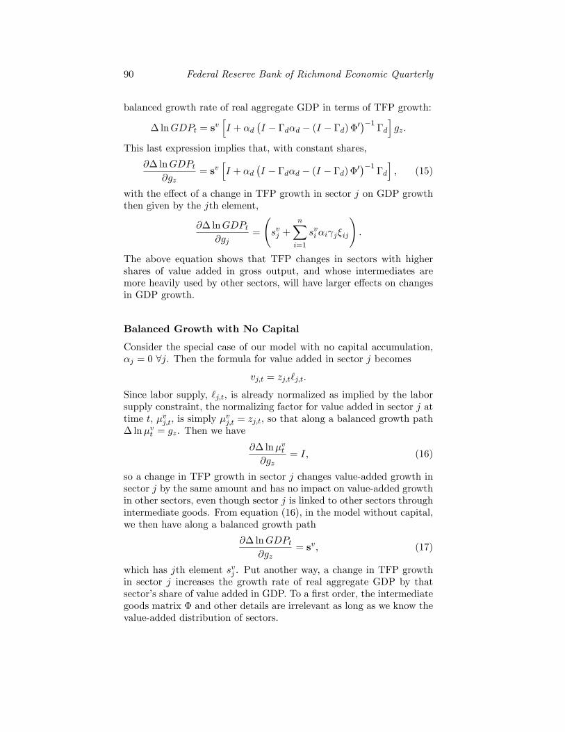
To see the extent to which changes in the usage of intermediategoods across sectors, summarized in Φ, have impacted the effect ofTFP growth changes in a sector on changes in the growth rate of GDP,we also recompute ∂∆ lnGDPt

∂gzusing the Φ matrix in 1948. Figure 2 plots

∂∆ lnGDPt∂gz

calculated in the benchmark using Φ from 2014 against thevalues calculated from 1948. Because we hold the other parametersconstant for each sector, any changes should result from changes inthe relative importance of sectors as intermediate goods suppliers toother sectors. As noted by Choi and Foerster (2017), there have been


Figure 1 Derivative of GDP Growth with Respect to SectorTFP Growth

significant changes in the US economy’s input-output network structureover this period. In particular, the Services sector is a markedly moreimportant supplier of intermediate goods in 2014 than it was in 1948,driven by the increasing centrality of financial services, real estate, andother industries within this sector. On the other hand, sectors suchas Manufacturing; Agriculture, Forestry, Fishing, and Hunting; andMining and Utilities declined in importance over this period.

Consistent with these observations, Services saw the largest ab-solute increase in ∂∆ lnGDPt

∂gzover this period, while Manufacturing saw

the largest absolute decrease, and Agriculture, Forestry, Fishing, andHunting saw the largest percentage decrease. On the other hand, be-cause ∂∆ lnGDPt

∂gzalso depends on the shares of each sector in total

nominal value added, a sector may decline in overall importance, asmeasured by its row total in Φ, over this period while still havingan increasing value of ∂∆ lnGDPt

∂gz. For example, Mining and Utilities

declines in overall importance between 1948 and 2014 but it is a muchmore important supplier of intermediates for the Manufacturing sector


Figure 2 Effect of TFP Growth on GDP Growth, 1948 Φ vs.2014 Φ

in 2014 than in 1948, largely explaining why Mining and Utilities seesa slight overall increase in ∂∆ lnGDPt

∂gz.

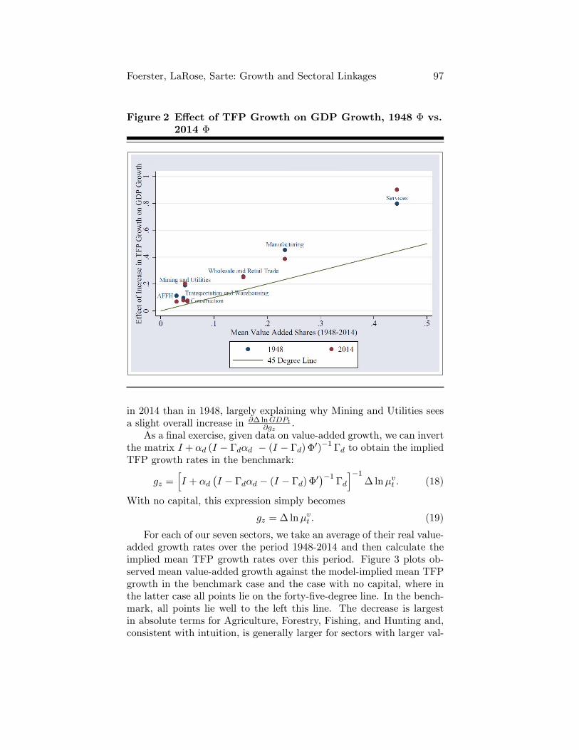
As a final exercise, given data on value-added growth, we can invertthe matrix I + αd (I − Γdαd − (I − Γd) Φ′)−1 Γd to obtain the impliedTFP growth rates in the benchmark:

gz =[I + αd

(I − Γdαd − (I − Γd) Φ′

)−1Γd

]−1∆ lnµvt . (18)

With no capital, this expression simply becomes

gz = ∆ lnµvt . (19)

For each of our seven sectors, we take an average of their real value-added growth rates over the period 1948-2014 and then calculate theimplied mean TFP growth rates over this period. Figure 3 plots ob-served mean value-added growth against the model-implied mean TFPgrowth in the benchmark case and the case with no capital, where inthe latter case all points lie on the forty-five-degree line. In the bench-mark, all points lie well to the left this line. The decrease is largestin absolute terms for Agriculture, Forestry, Fishing, and Hunting and,consistent with intuition, is generally larger for sectors with larger val-


Figure 3 Implied Mean TFP Growth, 1948-2014

ues of αj . The implied mean TFP growth for Mining and Utilities isjust 0.08 percent.

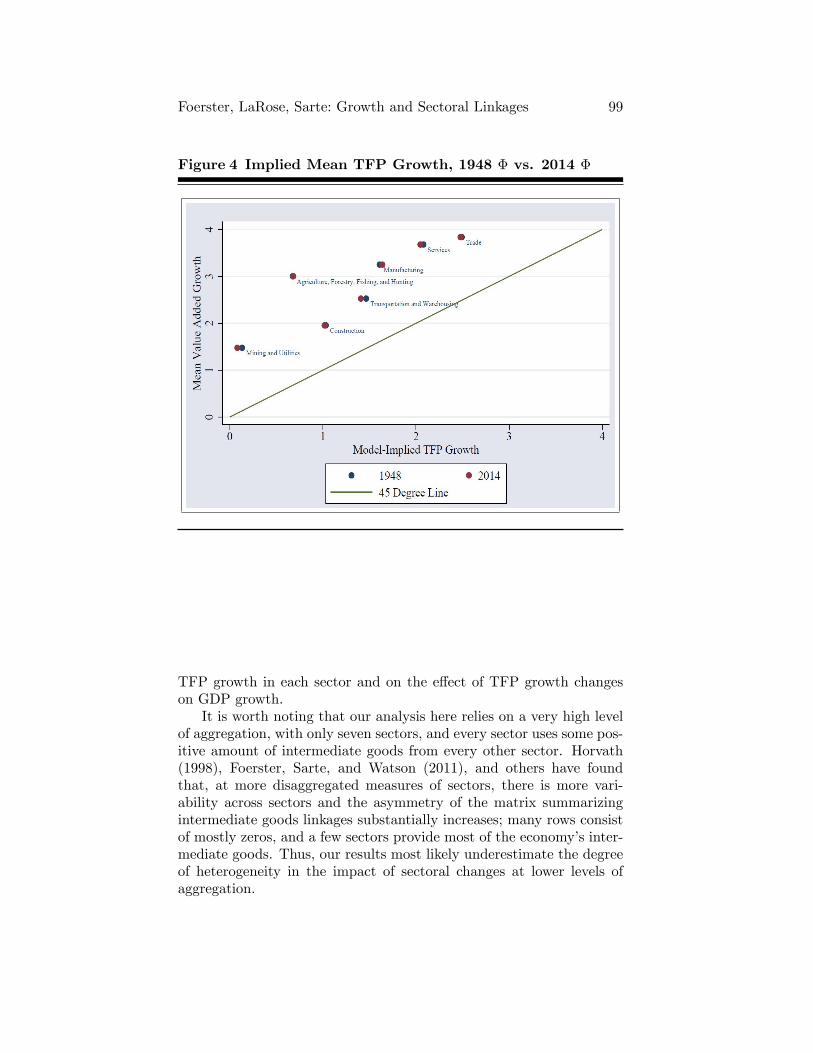
Additionally, for the benchmark case, we calculate implied meanTFP growth rates using the Φ matrix for 1948 and compare the resultsto those using the Φ matrix for 2014. As shown in Figure 4, changesin patterns of intermediate goods usage between 1948 and 2014 havevery little impact on implied mean TFP growth rates.

7. CONCLUSION

Our analysis suggests that linkages between sectors in intermediategoods, and capital intensities of different sectors, lead to substantialeffects of sector-specific TFP growth changes on value-added growth.TFP growth changes in sectors such as Manufacturing and Services,which account for a large share of the intermediate goods shares ofother sectors, have especially large impacts on value-added growth inother sectors. On the other hand, changes in the input-output structureof the US economy from 1948 to 2014 have had a modest impact on


Figure 4 Implied Mean TFP Growth, 1948 Φ vs. 2014 Φ

TFP growth in each sector and on the effect of TFP growth changeson GDP growth.

It is worth noting that our analysis here relies on a very high levelof aggregation, with only seven sectors, and every sector uses some pos-itive amount of intermediate goods from every other sector. Horvath(1998), Foerster, Sarte, and Watson (2011), and others have foundthat, at more disaggregated measures of sectors, there is more vari-ability across sectors and the asymmetry of the matrix summarizingintermediate goods linkages substantially increases; many rows consistof mostly zeros, and a few sectors provide most of the economy’s inter-mediate goods. Thus, our results most likely underestimate the degreeof heterogeneity in the impact of sectoral changes at lower levels ofaggregation.


REFERENCES

Acemoglu, Daron, Vasco M. Carvalho, Asuman Ozdaglar, and AlirezaTahbaz-Salehi. 2012. “The Network Origins of AggregateFluctuations.”Econometrica 80 (September): 1977—2016.

Atalay, Enghin. 2017. “How Important are Sectoral Shocks?”American Economic Journal: Macroeconomics 9 (October):254—80.

Baqaee, David R., and Emmanuel Farhi. 2018. “The MacroeconomicImpact of Microeconomic Shocks: Beyond Hulten’s Theorem.”Working Paper 23145. Cambridge, Mass.: National Bureau ofEconomic Research. (January).

Choi, Jason, and Andrew T. Foerster. 2017. “The ChangingInput-Output Network Structure of the U.S. Economy.”FederalReserve Bank of Kansas City Economic Review (Second Quarter):23—49.

Dupor, Bill. 1999. “Aggregation and Irrelevance in Multi-SectorModels.”Journal of Monetary Economics 43 (April): 391—409.

Foerster, Andrew T., Pierre-Daniel G. Sarte, and Mark W. Watson.2011. “Sectoral versus Aggregate Shocks: A Structural FactorAnalysis of Industrial Production.”Journal of Political Economy119 (February): 1—38.

Gabaix, Xavier. 2011. “The Granular Origins of AggregateFluctuations.”Econometrica 79 (May): 733—72.

Horvath, Michael. 1998. “Cyclicality and Sectoral Linkages:Aggregate Fluctuations from Independent Sectoral Shocks.”Review of Economic Dynamics 1 (October): 781—808.

Horvath, Michael. 2000. “Sectoral Shocks and AggregateFluctuations.”Journal of Monetary Economics 45 (February):69—106.

Hulten, Charles R. 1978. “Growth Accounting with IntermediateInputs.”Review of Economic Studies 45 (October): 511—18.

Long, John B. Jr., and Charles I. Plosser. 1983. “Real BusinessCycles.”Journal of Political Economy 91 (February): 39—69.

Lucas, Robert E. Jr. 1981. “Understanding Business Cycles.”InStudies in Business Cycle Theory. Cambridge, Mass.: MIT Press,215—39.


Miranda-Pinto, Jorge. 2018. “Production Network Structure, ServiceShare, and Aggregate Volatility.”Working Paper. (June).

Ngai, L. Rachel, and Christopher A. Pissarides. 2007. “StructuralChange in a Multisector Model of Growth.”American EconomicReview 91 (March): 429—43.

Pasten, Ernesto, Raphael Schoenle, and Michael Weber. 2018. “PriceRigidity and the Origins of Aggregate Fluctuations.”WorkingPaper 23750. Cambridge, Mass.: National Bureau of EconomicResearch. (August).

idiosyncratic sectoral growth, balanced growth, and ... · sectors), dupor found that aggregate...

Documents