identity, group conflict, and social preferences

Identity, Group Conflict, and Social Preferences

Rachel Kranton, Matthew Pease, Seth Sanders, and Scott Huettel*

April 2012

Abstract: This paper presents a novel experiment on group conflict. Subjects are divided into groups according to preferences on paintings, and subjects are divided into groups according to self-declared political affiliations and leanings. Using a unique within subject design, we find twenty percent of subjects destroy social welfare – at personal cost – when facing a subject outside their group. This effect relates to individual identities. In the political treatment, Democrats and Republicans, in contrast to Independents, behave more selfishly and competitively towards out-group members. The results show social preferences for fairness and social welfare maximization are not universal and depend on the social context. * The author order combines alphabetical order (the convention in economics) and lab director last (the convention in psychology & neuroscience norm). We are grateful to Jeff Butler, Pedro Rey-Biel and participants at Conference on the Economics of Interactions & Culture (EIEF), Ecole Polytechnique, Pompeu Fabra, Institute for Economic Analysis & Universitat Autònama de Barcelona, and Paris School of Economics for their comments. We thank the Social Science Research Institute at Duke for sponsoring our faculty fellows program in 2010-2011, “From Brain to Society (and Back),” and we are grateful to the Transdisciplinary Prevention Research Center (TPRC) at Duke for funding this project.

I. Introduction This paper presents a novel experiment on identity, group conflict, and social preferences. There

is now a storied academic literature that argues human beings are not purely selfish. Rather, people are

concerned about the well being of others when making decisions and allocating income. A series of

economic experiments has demonstrated that subjects will give up own income in order to achieve higher

social welfare and allocations that are more equitable. Yet this picture of preferences and allocation

decisions does not jibe with much of human history. While many cultural and religious traditions involve

charity and help to those less fortunate and redistribution is a feature of modern societies and democratic

governments, throughout time people have been unfair and cruel to others. Human history is full of

prolonged inter-group conflict, forced extraction of goods and labor, and genocide.1 Empirical research

in economics has demonstrated that ethnic divisions are related to lower levels of public goods,

dysfunctional institutions, and reduced growth.2

This paper delves into this apparent contradiction. We conduct a novel experiment to ask when

people behave selfishly, when they maximize social welfare, and when they destroy the payoffs of others.

The group division in our experiment is necessarily mild compared to the historical conflicts recalled

above. Yet, even in a congenial university environment, we uncover a significant amount of “status-

seeking” or “competitive behavior.”3 Using a unique within subject design, we find that twenty percent

of participants are concerned with relative payoffs to the extent that they destroy social welfare – at

personal cost – when facing a subject outside their group. This behavior is not punishment or retaliation

for non-cooperative behavior or “negative reciprocity.”4 Subjects in our experiment are not responding to

1 North, Wallace & Weingast (2009) are among those bold enough to tackle the sweep of human history. 2 Prominent studies include Easterly & Levine (1997), Alesina, Baqir, & Easterly (1999), Alesina & La Ferrara (2005), Miguel & Gugerty (2005). 3 With the recent exception of Iriberri & Rey-Biel (2011), experiments and proposed formulations of utility have largely ignored such behavior. The model proposed by Andreoni & Miller (2002) does not allow for status seeking behavior, and Bolton & Ockenfels (2000, p. 172, Assumption 3) rule out such behavior by assumption on the shape of their proposed utility function. Fehr & Schmidt’s (1999) utility function allows for the possibility of such behavior, but they do not include it in their analysis; they argue would not change equilibrium behavior in the games they consider (p. 824). 4 See, e.g., Fehr & Schmidt (1999), Fehr & Gächter (2000), Charness & Rabin (2002).

the choices of others; they are simply choosing allocations.5 Thus we find that there are a variety of

social preferences and these preferences depend critically on the social context.

This experiment thus advances the quest for uncovering the distribution of social preferences

(Fehr & Schmidt (2009)) and finds support for hypotheses concerning identity and economic outcomes

(Akerlof & Kranton (2000, 2010)). In this experiment, subjects allocate money to themselves and to

others in three conditions: an asocial control, a minimal group treatment, and a political group treatment.

In the minimal group treatment, following the classic method in social psychology, subjects are divided

into two groups according to their preferences over images and lines of poetry. In the political group

treatment, subjects are divided into two groups according to their self-declared political affiliations and

leanings. The asocial treatment serves as a control for both group treatments. The minimal group

treatment serves as a control for the political group treatment.

Following the work of Akerlof & Kranton (2000, 2010), we test whether a subject’s behavior

depends on his or her identity. Identity, here, as in social psychology, indicates an individual’s (self)-

assignment to a social category, or group. Examples of broad social categories in the real world are

gender, race, ethnicity, nationality, political party, etc. Experiments can draw on such existing identities,

or experiments can create social categories inside the laboratory, as in the minimal group treatment. The

premise of the latter is that studying subjects with temporary identities created in the laboratory serves as

a window on behavior outside the laboratory, where identities are longer lasting and more deeply held.

Our experiment combines these methods and tests two hypotheses. First, we test whether

subjects’ identities affect behavior. In particular, we test if subjects are less willing to allocate money to

subjects outside their group. Second, we test whether this effect depends on individual identities and

subjects’ affinities for their assigned group. We infer this affinity from subjects’ self-reported political

affiliations as Democrat, Republican, Independent, or None. An Independent assigned to the Democrat

5 Iriberri & Rey-Biel (2011) find that about 10% of subjects are “competitive” in a setting like our asocial condition. We find that about 5% are “competitive” in the asocial condition and 20% are competitive in group treatments when allocating income to subjects in the other group.

group would likely have less affinity for their assigned group than a Democrat assigned to the Democrat

group.

We find support for both hypotheses. In the minimal group treatment, subjects are more

competitive and more selfish when allocating money to out-group members. But in the political group

treatment, only Democrats and Republicans exhibit this behavior. Independents have significantly

different behavior, treating out-group subjects similarly to in-group subjects.

This study builds on two streams of experimental literature in economics: on social preferences

and on social identity. The work on social preferences often pits the theory of a “selfish economic man”

against a theory where people also have preferences over the payoffs of others. Charness & Rabin (2002)

introduce a series of games and method to estimate social preferences and conclude that subjects are not

purely selfish and exhibit preferences for social welfare maximization rather than aversion to inequity.

Fehr & Schmidt (1999) suggest that there might not be one way to describe people, as selfish or not, or

inequity averse or not, but rather there is a distribution of individual social preferences. Andreoni &

Miller (2002) find that indeed different individuals follow consistently different rules for the allocation of

payoffs. We find that, in the asocial condition, about 25% of subjects are “selfish,” they put almost no

weight on anyone’s payoffs but their own. About 37% of subjects have preferences to maximize social

welfare and 33% aim for fair allocations. The remaining 5% are “competitive;” they are willing to reduce

their own absolute payoffs in order to increase the difference between their payoffs and the other person’s

payoffs. These distributions change in the group treatments, indicating that social preferences are not

constant but depend on the social context. In particular, there is a significant increase in selfish behavior

and competitive behavior when allocating income to out-group subjects. In the minimal group treatment,

35% of subjects are selfish and 21% are competitive, with only 13% maximizing social welfare and 31%

striving for fair allocations. Thus well more than half of the subjects are neither fair nor social welfare

maximizing when facing out-group subjects.

In the area of social identity, several early experiments showed that the race or ethnicity of

subjects changes play in dictator and ultimatum games (e.g., Fershtman & Gneezy (2000), Glaeser,

Laibson, Scheinkman, and Souter (2000)). A recent set of experiments has studied social groups created

in the laboratory.6 Our paper is closest to Chen and Li (2009) who use a minimal group paradigm and

find that, on average, subjects are more likely to be social welfare maximizing towards in-group members.

Our paper is also close in spirit to, and supports the results of, Klor & Shayo (2010) who divide subjects

into two groups according to their university fields of study. Subjects are assigned gross incomes and

asked to vote over alternative redistributive tax schemes. They find that subjects vote more often for the

tax rate that favors in-group members.7 Our experiment finds a strong effect of the group treatment:

effect: on average, subjects are less fair when allocating to in-group members than out-group members,

which is similar to Chen & Li‘s (2009) results. This average hides the range of subject behavior. It hides

the prevalence of purely selfish behavior and the destructive behavior of subjects that emerges strongly in

the group context.

To uncover individual preferences, we use a finite mixing model, which is relatively new to

experimental economics. 8 We use the utility function proposed by Fehr & Schmidt (1999) and Charness

& Rabin (2002) and estimate parameters using a discrete choice maximum likelihood function and a finite

mixing model. The mixing model estimates “types” of subjects, where the parameters characterizing each

“type” are not assumed but are those that maximize the likelihood function. We can then interpret these

“types” according to the utility function: we find subjects are distinctly either “selfish,” “weak social

welfare maximizing,” “strong social welfare maximizing,” or “competitive.” Iriberri and Rey-Biel’s

(2011) recent contribution also studies the possibility that subjects adopt significantly different and

6 See Chen & Li (1999) and Akerlof & Kranton (2010) for extensive reviews of the experimental literature in economics and social psychology. 7 Klor & Shayo (2010) find further that subjects’ behavior in the experiment relates to answers to questions concerning redistribution in a post-experiment survey using an adaptation of questions from the World Values Survey. 8 To the best of our knowledge, Stahl and Wilson (1994) was the first use of finite mixture modeling in behavioral experiments. They and followers such as Bosch-Domenech et. al (2010) consider Beauty Contest games, estimating the proportion of subjects who reason at different levels. Harrison and Rutstrom (2009) and Conte et. al allow for a mixture of expected utility and prospect theory. Andersen et. al. (2011) allow for part of the population to behave according to traditional exponential discounting and the remainder to behave according to hyperbolic discounting.

distinct behavior in dictator games. They estimate four types using the Fehr & Schmidt (1999) and

Charness & Rabin (2002) linear utility that we also adopt. 9

We take a further step and classify individual subjects into types in a way consistent with the

mixing distribution (Nagin (2005)). We construct a posterior probability that an individual subject is of

certain type and assign individuals to the type with the greatest posterior probability. To our knowledge

the present study is the only one in behavioral economics that takes this next step and combines this

classification with demographics and other subject-specific data to study the sources of individual

variation.10 We use this classification to test the identity hypotheses discussed above. We also study how

political ideology and demographic characteristics relate to individual behavior in different treatments.

We uncover, in particular, a correlation between social preferences and political ideology; subjects who

support “small government” are significantly more selfish than other subjects.

This paper is organized as follows. Section II describes our experiment in detail. Section

III provides the theoretical framework and empirical strategy for analyzing the data. We report

the behavioral results in Section IV. Section V concludes.

II. The Experiment

The experiment was conducted in the Duke Center for Cognitive Neuroscience, which

follows the same protocols as laboratories in experimental economics, in particular the protocol

of no deception. The experiment involved 141 subjects drawn from the Duke University

community. Summary demographic characteristics of the subjects are presented in the Appendix.

9 Econometrically the present paper differs from Iriberri & Rey-Biel (2011) in that we use the mixture model to calculate the posterior probability that an individual is a particular type and use these posterior probabilities to assign each individual to a type. We then determine the demographic and other factors that are associated with each type. Substantively, the goals of the papers are also different. Iriberri & Rey-Biel study how revealing the distribution of play changes future play, and they take great care to minimize any interpersonal influences that could stimulate other-regarding behavior. The purpose of our experiment, in contrast, is to test how different social contexts affect other-regarding behavior. 10 Klor & Shayo (2010) classify subjects into types according to the individual utility parameter estimates, as in Andreoni & Miller (2002). They then relate this type-classification to individual attributes and answers to survey questions.

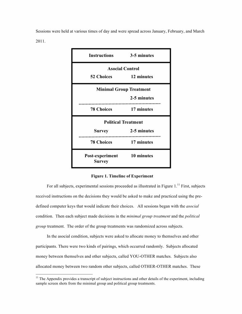
Sessions were held at various times of day and were spread across January, February, and March

2011.

Figure 1. Timeline of Experiment

For all subjects, experimental sessions proceeded as illustrated in Figure 1.11 First, subjects

received instructions on the decisions they would be asked to make and practiced using the pre-

defined computer keys that would indicate their choices. All sessions began with the asocial

condition. Then each subject made decisions in the minimal group treatment and the political

group treatment. The order of the group treatments was randomized across subjects.

In the asocial condition, subjects were asked to allocate money to themselves and other

participants. There were two kinds of pairings, which occurred randomly. Subjects allocated

money between themselves and other subjects, called YOU-OTHER matches. Subjects also

allocated money between two random other subjects, called OTHER-OTHER matches. These

11 The Appendix provides a transcript of subject instructions and other details of the experiment, including sample screen shots from the minimal group and political group treatments.

Instructions 3-5 minutes

Asocial Control

12 minutes

2

Survey

2-5 minutes

78 Choices 17 minutes

Minimal Group Treatment

52 Choices

Survey 2-5 minutes

78 Choices 17 minutes

Political Treatment

Post-experiment Survey

10 minutes

latter matches involved no loss or gain to the subject who made the decision.

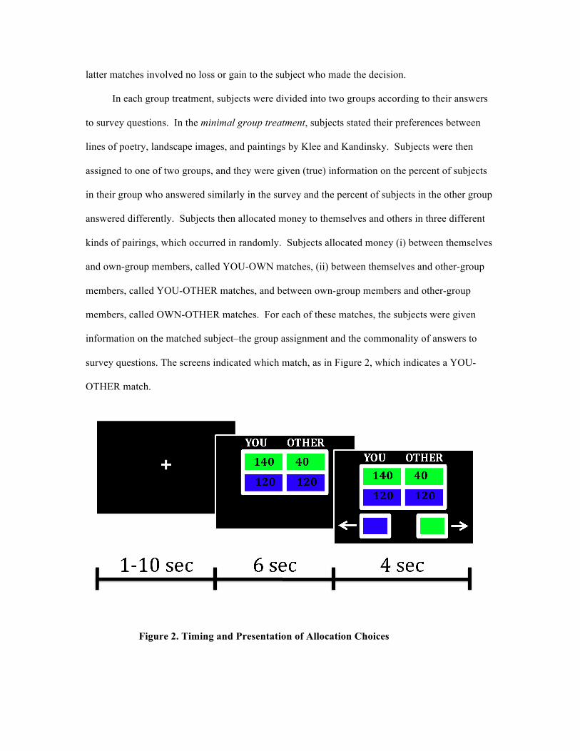
In each group treatment, subjects were divided into two groups according to their answers

to survey questions. In the minimal group treatment, subjects stated their preferences between

lines of poetry, landscape images, and paintings by Klee and Kandinsky. Subjects were then

assigned to one of two groups, and they were given (true) information on the percent of subjects

in their group who answered similarly in the survey and the percent of subjects in the other group

answered differently. Subjects then allocated money to themselves and others in three different

kinds of pairings, which occurred in randomly. Subjects allocated money (i) between themselves

and own-group members, called YOU-OWN matches, (ii) between themselves and other-group

members, called YOU-OTHER matches, and between own-group members and other-group

members, called OWN-OTHER matches. For each of these matches, the subjects were given

information on the matched subject–the group assignment and the commonality of answers to

survey questions. The screens indicated which match, as in Figure 2, which indicates a YOU-

OTHER match.

Figure 2. Timing and Presentation of Allocation Choices

The political treatment began with a survey of subjects’ political affiliations and opinions.

Subjects were first asked their political affiliations as Democrat, Republican, Independent, or

None. They were then asked to refine their political leanings—strong, moderate, or closer to

Democrat, closer to Republican. Subjects were then asked their opinions on issues that were

dividing the political spectrum in the United States at that time, as well as their preferred media

outlets.12 Based on their answers, subjects were assigned to two groups, called a Democratic

group and a Republican group. Subjects were given information on the percent of subjects in

their assigned group that made similar chooses in the survey and the percent of subjects in the

other group that expressed different opinions. Note again that there was no deception in this

experiment, and we divided the subjects into groups according to an algorithm that would place

Democrat and Democrat-leaning subjects in the Democrat group and Republican and Republican-

leaning subjects in the Republican group. The information the subjects received was true data

about the opinions held in both groups. Subjects were then asked to allocate money to

themselves and to participants in their own or other group, as well between two subjects in their

own group and the other group. The screens indicating YOU-OWN, YOU-OTHER, and OWN-

OTHER had exactly the format as in the minimal group treatment.13

For each kind of match, subjects were presented with twenty-six different 2x2 allocation

matrices. The collection of these matrices can be found in the Appendix, and Figure 2 provides

an example. Following Charness & Rabin (2002), we constructed these matrices to capture three

basic types of social preferences. The subjects could, at possible expense to self, (1) increase

fairness, (2) increase social welfare, or (3) increase own status, i.e., the difference between their

own payoffs and the other’s payoffs (also called “status seeking” or “competitive” behavior).

12 The issues were abortion, illegal immigration, large government, gay marriage, and the Bush tax cuts. The Appendix provides summary statistics of the political affiliations, leanings, and opinions of the subject pool. 13 The Appendix describes the procedure and the information subjects received about the other participant’s answers to survey questions. In all other ways the matching is anonymous, and the recipient could be from another session of the experiment.

The matrices could involve more than one motive a time: For example, in the matrix in Figure 2,

a subject who picked the bottom vector would both be increasing social welfare and reducing

inequity at a personal cost. The econometric estimation of social preferences distinguishes

among these motives. The total of twenty-six different matrices were presented to each subject in

random order, and in random matches, in each condition. The vectors within each matrix were

randomized, so that sometimes the top vector gave the subject more money than the bottom

vector, or vice versa. The colors of the vectors, blue and green, as well as the left and right keys,

were all randomized.14

In addition to the show-up fee of $6, subjects received payment for one choice selected at

random from each of the three sections of the experiment—asocial, minimal group, and political.

The points in the matrix were translated into dollars according to a conversion factor and subjects

earned on average $15 for the one-hour sessions.

Before analyzing the results, we discuss possible experimenter demand effects. Within

subject designs, it has been argued, are subject to experimenter-demand effects, where the

subjects try to behave according to what they think the experimenter desires of them. In this

experiment, for example, subjects might think that we (the experimenters) are calling attention to

group divisions and therefore might try to act according to what they think we want them to do.

We have several responses to this criticism. First, the aim of this experiment is precisely to

see how people behave when groups are made salient. Many real-world actors create and exploit

group divisions to their own advantage. And indeed in political campaigns, actors try to

accentuate the difference between voters. Second, if there is a demand effect, there is no general

agreement among subjects as to what the demand is, as there is a wide range of subject behavior.

Third, subjects’ choices are correlated with their stated political opinions (as opposed to their

party affiliations), as measured by responses to questions on large vs. small government,

14 In addition, at the end of the asocial condition, subjects were asked to distribute points using tasks similar to those Andreoni & Miller (2002). This objective is to compare the outcomes of the binary choices in our experiment to those in Andreoni & Miller (2002).

government programs, and tax policy. These questions appeared either one-third or two-thirds of

the way into the experiment and were interspersed among eight questions on political positions,

political affiliation and news outlets. Finally, if there is a demand effect, there is no reason to

believe that the demand effect would be different for the minimal group treatment and the

political treatment. Hence, we control for any demand effect when comparing those two

treatments.

III. A Bird’s Eye View: Subjects’ Overall Choices across Conditions

In our first pass through the data, we look at the subjects’ overall choices of different

allocations. We report the percentage of the population that chooses fair vs. competitive vs.

social welfare maximizing allocations in each social condition. In the next section, we delve into

the individual variation behind these aggregate patterns.

III.A. Summary Statistics

Figure 3 presents the summary statistics of subjects’ choices in each condition. In each

decision, subject i choses one of two vectors (πi, πj) and (πʹ′i, πʹ′j). When a subject chooses (πʹ′i, πʹ′j),

we say the choice is consistent with being “selfish” if πi > πʹ′i. The choice is consistent with being

“fair” if ⏐πʹ′i − πʹ′j ⏐<⏐πi,− πj⏐. The choice is consistent with “maximizing social welfare” if πʹ′i +

πʹ′j > πi,+ πj. Finally, the choice is “competitive” if πʹ′i − πʹ′j > πi,− πj. Note that choice of (πʹ′i, πʹ′j)

could be consistent with several of these characterizations at the same time.

Figure 3 shows the percent of choices that are consistent with being “selfish,” “fair,”

“social maximizing,” and “competitive,” in each condition, for YOU-OTHER and YOU-OWN

matches. We see immediately that the asocial YOU-OTHER matches and the group YOU-OWN

matches follow similar patterns, with about 73% of choices consistent with “selfish,” 63%

percent of choices consistent with “social welfare maximization,” 55% consistent with “fairness,”

and 45% consistent with “competitiveness.” Figure 3 further shows the divergence between

YOU-OWN matches and YOU-OTHER matches in the group treatments. This difference is

particularly strong in the political treatment, where in YOU-OTHER matches only 52% of

choices are consistent with “social welfare maximization” and 47% consistent with “fairness,”

while 60% are consistent with “competitiveness.” These summaries are consistent with Charness

& Rabin’s (2002) and Chen & Li’s (2009) results for binary choice two-player games.15

Figure 3. Summary Statistics Percent of Choices consistent with

Selfishness, Social Welfare Maximization, Fairness, and Competitiveness

III.B. Price Sensitivity: Tradeoffs between Own Payoffs and Social Objective

We study next how much subjects are willing to give up in order to achieve a particular

social objective. We study the tradeoffs between own payoffs and others’ payoffs. For purposes

of analysis, we will represent the choice between vectors (πi, πi) and (πʹ′j, πʹ′j) as a normalized

matrix:

15 See Charness & Rabin (2002, Table 1, pg. 829) and Chen & Li (2009, Table A1, p. 454-455).

€

πi

€

π j

€

′ π i

€

′ π j

where the decision-maker, i, earns weakly more money in the top vector than the bottom. (As

reported above, in the actual experiment the rows were randomized.) With this formulation, a

subject who chooses the bottom vector chooses (weakly) less money for himself. Let Δπi, = πi−πʹ′i

be the loss to subject i from choosing the bottom vector; by definition Δπi, ≥ 0. A subject who

chooses a bottom vector (weakly) gives up some of his own money and achieves a social

objective. We again consider three objectives:

(1) FAIRNESS: The bottom allocation is fairer when ⏐πʹ′i − πʹ′j ⏐<⏐πi,− πj⏐.

(2) SOCIAL WELFARE: The bottom allocation has higher social welfare when πʹ′i + πʹ′j > πi,+ πj .

(3) COMPETITIVE/STATUS: The bottom allocation has higher status for i when πʹ′i − πʹ′j > πi,− πj .

We categorize the twenty-six allocation decisions according to whether choosing the

bottom vector achieves (1), (2), or (3). Note that choice of the bottom vector can be consistent

with multiple objectives.

We order the allocations according to the relative personal cost and social benefits to

subject i. We construct a “bang-for-the-buck” measure; an allocation is relatively more expensive

for i when ⏐Δπi/(Δπi−Δπj) ⏐is larger⎯the subject would have to give up relatively more of own

money to achieve an increase in the social objective. We examine subjects’ choices across social

conditions, distinguishing between the matrices where i earns more than j and the matrices where

j earns more than i. We do so since previous work indicates that subjects are more willing to give

to others when they earn more than the other; i.e., πI > πj, then when they earn less πi,< πj.

Figure 4 compares subjects’ choices, in aggregate, across different conditions. On the x-

axis in each figure, we order the matrices according to the measure Δπi,/(Δπi,−Δπj,).

The matrices to the right of the origin, then, have bottom vectors that are fairer and/or have higher

social welfare. The further the matrix is from the origin, the relatively more it costs for i to be

fair or social welfare maximizing. The matrices to the left of the origin have bottom vectors that

have higher status for subject i. The further the matrix is from the origin, the relatively more it

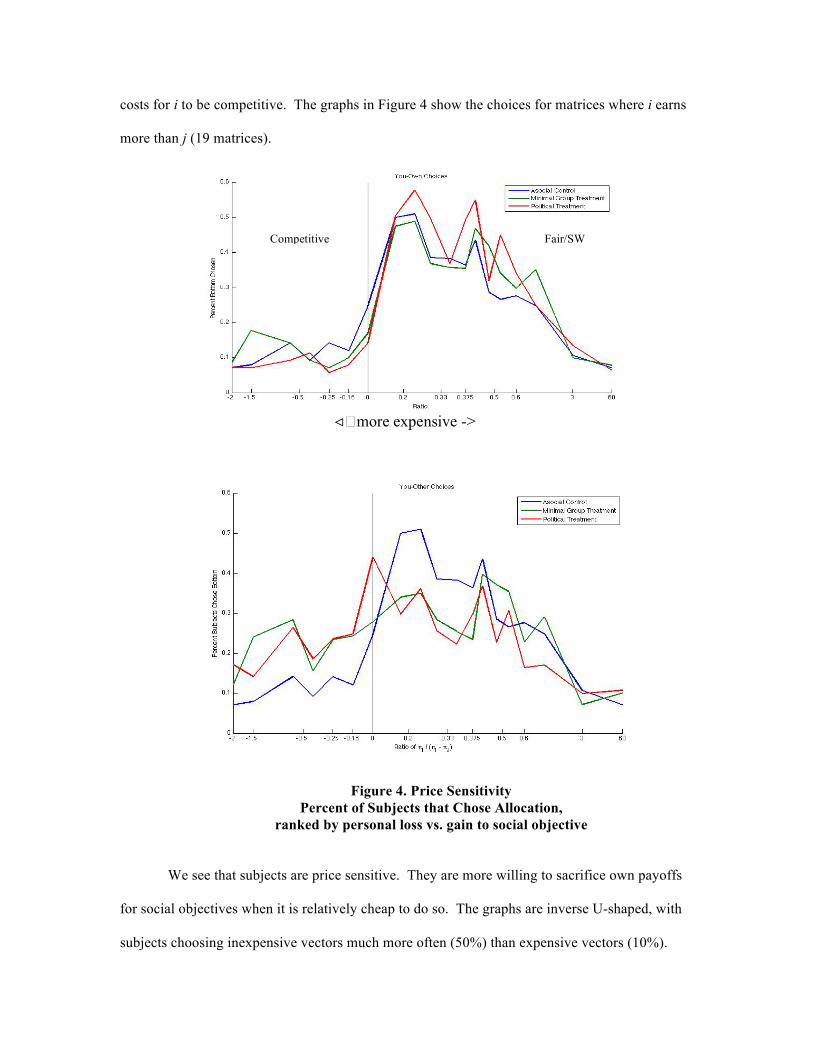
costs for i to be competitive. The graphs in Figure 4 show the choices for matrices where i earns

more than j (19 matrices).

Figure 4. Price Sensitivity Percent of Subjects that Chose Allocation,

ranked by personal loss vs. gain to social objective

We see that subjects are price sensitive. They are more willing to sacrifice own payoffs

for social objectives when it is relatively cheap to do so. The graphs are inverse U-shaped, with

subjects choosing inexpensive vectors much more often (50%) than expensive vectors (10%).

Competitive Fair/SW

1

�more expensive ->

We further observe the group divisions affect subjects’ willingness to pay for social

objectives. There is little difference for group treatment YOU-OWN matches and the asocial

control, seen in the top panel of Figure 4. But the YOU-OTHER trials, shown in the bottom

panel, indicate less willingness to pay for fair or social welfare maximizing allocations, and

greater willingness to pay for competitive allocations. Here it appears there is little difference

between the political group and the asocial condition.

III.C. Response Time: Population Averages

IV. Social Preferences: Population vs. Distribution of Individuals

In this section we identify patterns in individual behavior. We do so by estimating social

preferences and relate these patterns to individual characteristics and answers to survey questions.

IV.A. Estimation Strategy

To analyze social preferences, we first follow the standard method in this field: we posit a

utility function for choices over allocations and analyze the discrete choice data. We estimate the

parameters of the utility function using a maximum likelihood logit regression. It should be noted

that results of this kind obviously depend on the specific form of the utility function. For

comparison purposes, we adapt the Fehr & Schmidt (1999) and Charness & Rabin (2002) linear

utility function, which allows us to see a range of behavior, including competitive behavior.16

The goal is to test, given this functional form, whether there are individual differences in utility

parameters, which indicate different types of social preferences. We study the distributions of

types in different social contexts social identity.

16 We do not argue that this utility function is the best representation of people’s motivations. For example, since it is linear, marginal utility of own income is constant. We adopt it following Charness & Rabin (2002) who show that, nonetheless, it is a useful summary of social preferences.

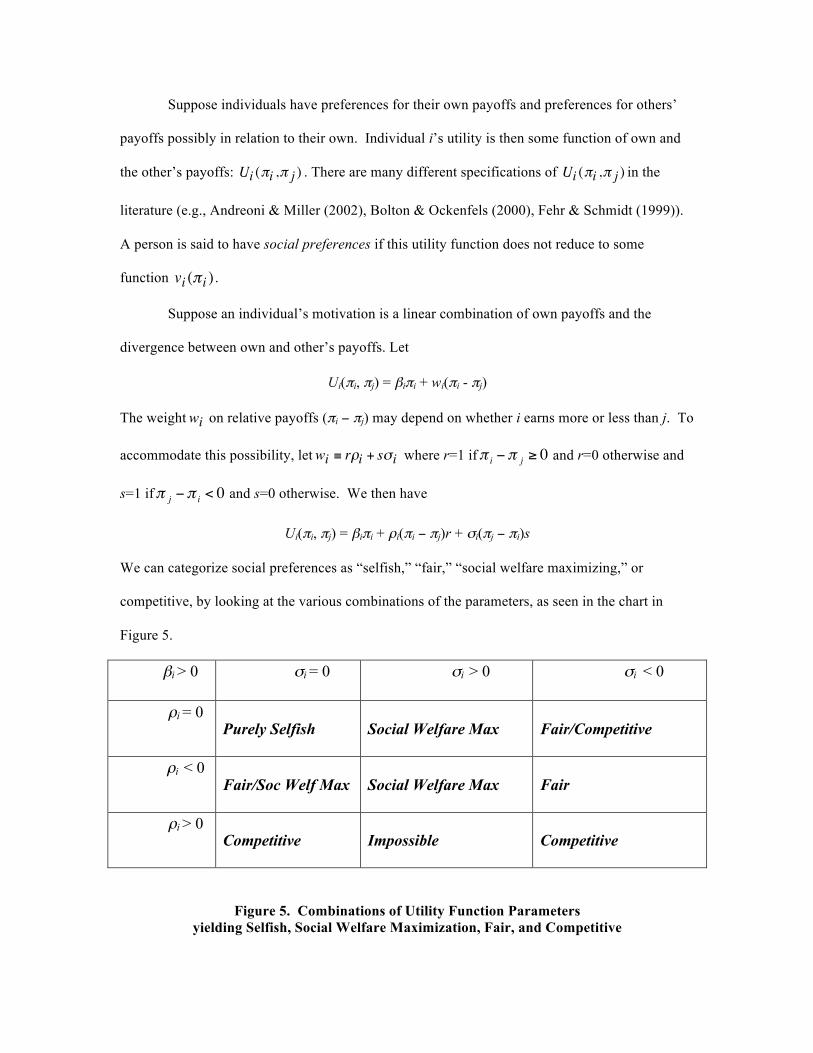
Suppose individuals have preferences for their own payoffs and preferences for others’

payoffs possibly in relation to their own. Individual i’s utility is then some function of own and

the other’s payoffs: . There are many different specifications of in the

literature (e.g., Andreoni & Miller (2002), Bolton & Ockenfels (2000), Fehr & Schmidt (1999)).

A person is said to have social preferences if this utility function does not reduce to some

function .

Suppose an individual’s motivation is a linear combination of own payoffs and the

divergence between own and other’s payoffs. Let

Ui(πi, πj) = βiπi + wi(πi - πj)

The weight on relative payoffs (πi − πj) may depend on whether i earns more or less than j. To

accommodate this possibility, let where r=1 if and r=0 otherwise and

s=1 if and s=0 otherwise. We then have

Ui(πi, πj) = βiπi + ρi(πi − πj)r + σi(πj − πi)s

We can categorize social preferences as “selfish,” “fair,” “social welfare maximizing,” or

competitive, by looking at the various combinations of the parameters, as seen in the chart in

Figure 5.

βi > 0 σi = 0 σi > 0 σi < 0

ρi = 0 Purely Selfish

Social Welfare Max

Fair/Competitive

ρi < 0 Fair/Soc Welf Max

Social Welfare Max

Fair

ρi > 0 Competitive

Impossible

Competitive

Figure 5. Combinations of Utility Function Parameters yielding Selfish, Social Welfare Maximization, Fair, and Competitive

€

Ui (πi ,π j )

€

Ui (πi ,π j )

€

vi (π i )

€

wi

€

wi ≡ rρi + sσi

€

π i −π j ≥ 0

€

π j −π i < 0

Given β > 0, if, ρ = σ = 0 then there are no social preferences; people are purely selfish. If,

however, ρ > 0 and σ > 0, then the social preferences are for social welfare maximization, since

utility is always increasing in both πi and πj. If however ρ < 0 and σ < 0, then social preferences

are for “fairness,” since utility is always decreasing when i more earns than j or vice versa. When

ρ > 0 and σ < 0, then utility always increases when i earns more than j; this combination

indicates a social preference for status, and we say people with these preferences are competitive.

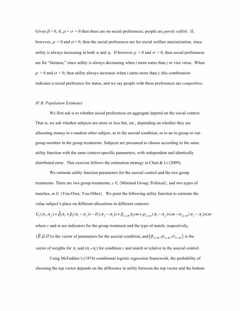
IV.B. Population Estimates

We first ask is to whether social preferences on aggregate depend on the social context.

That is, we ask whether subjects are more or less fair, etc., depending on whether they are

allocating money to a random other subject, as in the asocial condition, or to an in-group or out-

group member in the group treatments. Subjects are presumed to choose according to the same

utility function with the same context-specific parameters, with independent and identically

distributed error. This exercise follows the estimation strategy in Chen & Li (2009).

We estimate utility function parameters for the asocial control and the two group

treatments. There are two group treatments, c ∈ {Minimal Group, Political}, and two types of

matches, m ∈ {You-Own, You-Other}. We posit the following utility function to estimate the

value subject’s place on different allocations in different contexts:

where c and m are indicators for the group treatment and the type of match, respectively,

is the vector of parameters for the asocial condition, and is the

vector of weights for πi, and (πi,−πj,) for condition c and match m relative to the asocial control.

Using McFadden’s (1974) conditional logistic regression framework, the probability of

choosing the top vector depends on the difference in utility between the top vector and the bottom

€

Ui (π i ,π j ) = β iπ i + ρ i (π i − π j )r −σ i (π j − π i )s+ βi,c,mπ icm + ρi,c,m (π i − π j )rcm −σ i,c,m (π j − π i )scm

€

(β ,ρ ,σ )

€

βi,c,m ,ρi,c,m ,σ i,c,m( )

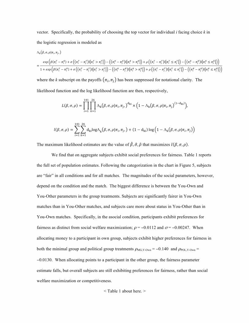
vector. Specifically, the probability of choosing the top vector for individual i facing choice k in

the logistic regression is modeled as

Λ! 𝛽,𝜎, 𝜌|𝜋! ,𝜋! ,

=𝑒𝑥𝑝 𝛽 𝜋!! − 𝜋!! + 𝜎 𝜋!! − 𝜋!! Ι 𝜋!! > 𝜋!! − 𝜋!! − 𝜋!! Ι 𝜋!! > 𝜋!! + 𝜌 𝜋!! − 𝜋!! Ι 𝜋!! ≤ 𝜋!! − 𝜋!! − 𝜋!! Ι 𝜋!! ≤ 𝜋!!

1 + 𝑒𝑥𝑝 𝛽 𝜋!! − 𝜋!! + 𝜎 𝜋!! − 𝜋!! Ι 𝜋!! > 𝜋!! − 𝜋!! − 𝜋!! Ι 𝜋!! > 𝜋!! + 𝜌 𝜋!! − 𝜋!! Ι 𝜋!! ≤ 𝜋!! − 𝜋!! − 𝜋!! Ι 𝜋!! ≤ 𝜋!!

where the k subscript on the payoffs 𝜋! ,𝜋! has been suppressed for notational clarity. The

likelihood function and the log likelihood function are then, respectively,

𝐿 𝛽,𝜎, 𝜌 = Λ! 𝛽,𝜎, 𝜌|𝜋! ,𝜋! ,!!"

!"

!!!

!"!

!!!

× 1 − Λ! 𝛽,𝜎, 𝜌|𝜋! ,𝜋!!!!!" ,

𝑙 𝛽,𝜎, 𝜌 = d!"logΛ! 𝛽,𝜎, 𝜌|𝜋! ,𝜋! , + 1 − d!"

!"

!!!

log 1 − Λ! 𝛽,𝜎, 𝜌|𝜋! ,𝜋!

!"!

!!!

The maximum likelihood estimates are the value of 𝛽,𝜎, 𝜌 that maximizes 𝑙 𝛽,𝜎, 𝜌 .

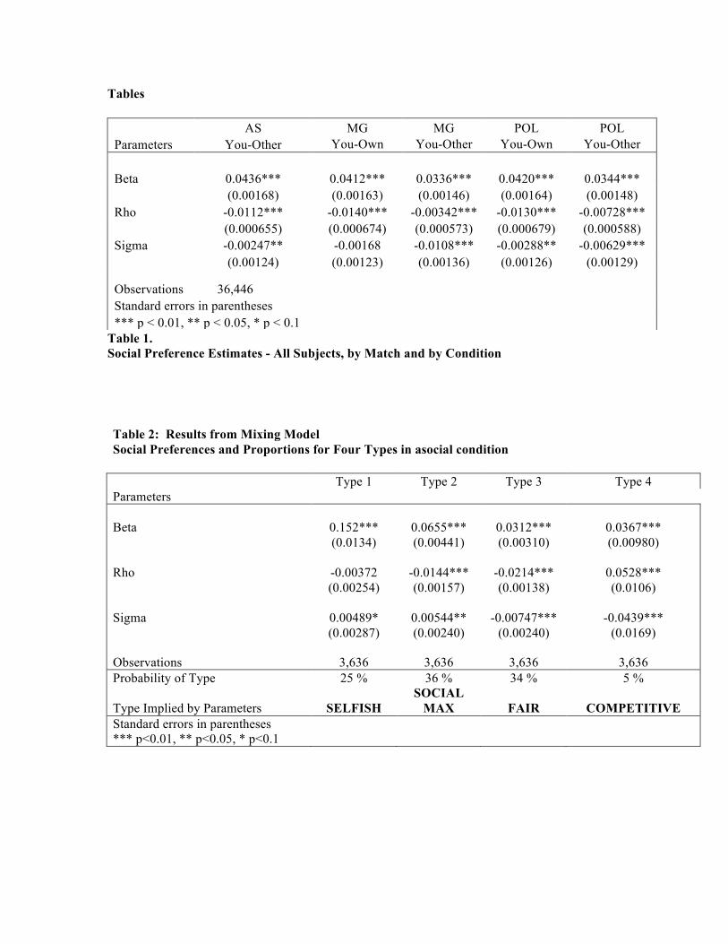
We find that on aggregate subjects exhibit social preferences for fairness. Table 1 reports

the full set of population estimates. Following the categorization in the chart in Figure 5, subjects

are “fair” in all conditions and for all matches. The magnitudes of the social parameters, however,

depend on the condition and the match. The biggest difference is between the You-Own and

You-Other parameters in the group treatments. Subjects are significantly fairer in You-Own

matches than in You-Other matches, and subjects care more about status in You-Other than in

You-Own matches. Specifically, in the asocial condition, participants exhibit preferences for

fairness as distinct from social welfare maximization; ρ = −0.0112 and σ = −0.00247. When

allocating money to a participant in own group, subjects exhibit higher preferences for fairness in

both the minimal group and political group treatments ρMG,Y-Own = −0.140 and ρPOL,Y-Own =

−0.0130. When allocating points to a participant in the other group, the fairness parameter

estimate falls, but overall subjects are still exhibiting preferences for fairness, rather than social

welfare maximization or competitiveness.

< Table 1 about here. >

IV.C. Distributions of Social Preferences

In this section we estimate the distribution of social preferences. Rather than presume

there is a single set of utility function parameters that represent the preferences of all individuals,

we allow for the possibility that there are different “types” of people, where each “type” has

distinct preferences. With our design, we essentially have panel data (multiple choices for each

individual), and thus it is possible to estimate a finite mixture model, also called a latent class

model. A finite mixture model allow there to be a finite number of “types” in the population,

where each “type” is characterized by different parameter values. We first find four “types” that

best characterize the data. We then classify individuals into types and estimate the precision with

which an individual’s choice fit with the estimated type parameters. As we will see below,

almost individuals can be classified into one of the four types with probabilities close to 99%.

We estimate four types. Four types is the minimum number that would allow us to

identify the four distinct motives modeled in the utility function. Five or more types leads to very

small number of individuals in some types. While we estimate four types, it is important to

emphasize that it is the data that gives us the utility parameters for each type. That is, there is no

presumption, a priori, that the types will map into the four different motives outlined above.

Building on the above specification for the likelihood functions, each parameter of the

utility function is now subscripted by t to indicate a type. That is, 𝛽! ,𝜎! , 𝜌! are the three main

parameters of interest for type t. We further estimate the fraction of the population of each type;

that is, the prior probability of an individual being of a particular type. The mixture model then

has a total of fifteen parameters to estimate: three utility parameters for each of the four types and

three mixing probabilities, where the complement gives us the probability of the fourth type.

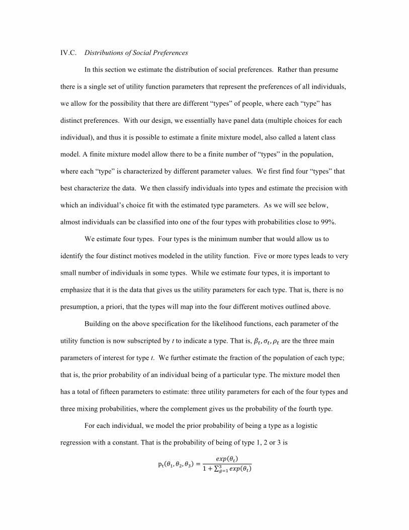
For each individual, we model the prior probability of being a type as a logistic

regression with a constant. That is the probability of being of type 1, 2 or 3 is

p! 𝜃!, 𝜃!, 𝜃! =𝑒𝑥𝑝 𝜃!

1 + 𝑒𝑥𝑝 𝜃!!!!!

and p! 𝜃!, 𝜃!, 𝜃! = 1 − p! + p! + p! . The log likelihood function is then

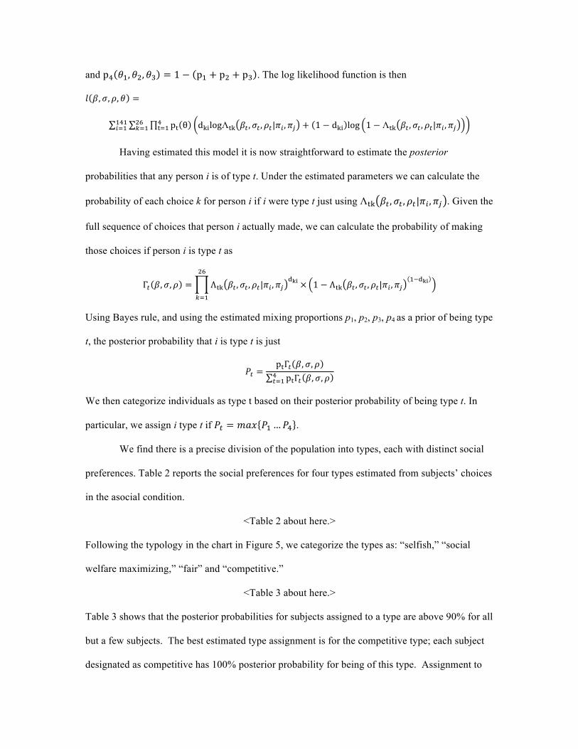
𝑙 𝛽,𝜎, 𝜌, 𝜃 =

p! θ d!"logΛ!" 𝛽! ,𝜎! , 𝜌!|𝜋! ,𝜋! + 1 − d!" log 1 − Λ!" 𝛽! ,𝜎! , 𝜌!|𝜋! ,𝜋!!!!!

!"!!!

!"!!!!

Having estimated this model it is now straightforward to estimate the posterior

probabilities that any person i is of type t. Under the estimated parameters we can calculate the

probability of each choice k for person i if i were type t just using Λ!" 𝛽! ,𝜎! , 𝜌!|𝜋! ,𝜋! . Given the

full sequence of choices that person i actually made, we can calculate the probability of making

those choices if person i is type t as

Γ! 𝛽,𝜎, 𝜌 = Λ!" 𝛽! ,𝜎! , 𝜌!|𝜋! ,𝜋!!!"

!"

!!!

× 1 − Λ!" 𝛽! ,𝜎! , 𝜌!|𝜋! ,𝜋!!!!!"

Using Bayes rule, and using the estimated mixing proportions p1, p2, p3, p4 as a prior of being type

t, the posterior probability that i is type t is just

𝑃! =p!Γ! 𝛽,𝜎, 𝜌p!Γ! 𝛽,𝜎, 𝜌!

!!!

We then categorize individuals as type t based on their posterior probability of being type t. In

particular, we assign i type t if 𝑃! = 𝑚𝑎𝑥 𝑃!…𝑃! .

We find there is a precise division of the population into types, each with distinct social

preferences. Table 2 reports the social preferences for four types estimated from subjects’ choices

in the asocial condition.

<Table 2 about here.>

Following the typology in the chart in Figure 5, we categorize the types as: “selfish,” “social

welfare maximizing,” “fair” and “competitive.”


Table 3 shows that the posterior probabilities for subjects assigned to a type are above 90% for all

but a few subjects. The best estimated type assignment is for the competitive type; each subject

designated as competitive has 100% posterior probability for being of this type. Assignment to

“selfish” is almost as precise, with all subjects but one having above a 90% posterior probability

of being of this type. “Social welfare maximizers” and “fair” types are only a bit less precisely

assigned; this slightly smaller precision is due to the fact that these types exhibit somewhat

similar behavior, which is less distinctive than “selfish” and “competitive” behavior.

This estimation gives a precise distribution of the social preferences in our population. In

the asocial condition, 25% of subjects are selfish, 36% are social welfare maximizers, 34% are

fair, and 5% are competitive.

We now turn to our tests of the identity hypotheses; we ask how group divisions affect

the distribution of types in the population. The premise is that people may switch from one “type”

to another “type” given the particular social context. A person who is “fair” in the asocial

condition, for example, could be “selfish” in the group treatment when allocating income to

someone outside his group. We classify each individual’s behavior into types in each of the

group treatments, by match, as seen in Table 4.

<Tables 4 and 5 about here.>

Table 5 provides the cross-tabulations, showing the switching described above; it gives the

number of subjects that are type x in the asocial condition but type y in a group treatment, by

match.

Looking at the changes in behavior across condition, we first see that selfish types in the

asocial condition tend to stay as selfish across conditions and matches. We also see that

competitive types in the asocial condition are competitive across conditions and matches. For

these subjects, their social preferences do not depend on the particular social context.

For the rest of the subjects, social context does matter. Across conditions (asocial vs.

groups) we see that many subjects who are “social welfare-maximizing” or “fair” become

“competitive” in group treatment YOU-OTHER matches. Within each group treatment, there is a

similar pattern. For both the minimal group treatment and the political treatment, most “selfish”

subjects in YOU-OWN continue to be “selfish” in YOU-OTHER matches. But there are many

subjects who switch from “fair” or “social welfare maximizing” in YOU-OWN matches to the

“competitive” in YOU-OTHER matches.

We find that these switches lead to statistically significantly distributions of types for

each combination of condition and match. Table 6 provides the Chi-squared tests.


We can discern a pattern in these differences. Comparing the asocial control to the group

treatments, we see the difference is relatively small for You-Own matches. There is a shift from

social welfare maximizing to fairness: In MG-You-Own matches, compared to the asocial

condition, fewer subjects are “social welfare maximizers,” 18% vs. 37%, and more subjects are

“fair,” 50% vs. 33%. For You-Other matches, on the other hand, there is a large difference in the

distributions; many more subjects are “selfish” and “competitive.” For MG-You-Other matches,

35% of subjects are “selfish” and 21% are competitive. For POL-You-Other matches, 30% of

subjects are “selfish” and 16% are competitive. Fewer subjects are “social welfare maximizers,”

with only 13% in MG You-Other matches and 21% in POL-You Other matches.

Within each group treatment, we easily see that more subjects are competitive vis a vis

out-group members than in-group members. In the minimal group treatment, in You-Other

matches, 21% of subjects are competitive, compared to 1% in You-Other matches. The pattern in

the political treatment is a similar, though less pronounced (16% vs. 4%). For You-Other

matches, there is also less “social welfare maximizing” and “fair” behavior.

These results support the basic hypothesis that behavior towards self and others depends

on social identity and social context. In summary, overall subjects are “fair,” and subjects are

more “fair” or less “fair,” depending on whether they face an in-group vs. out-group member.

But this average behavior masks the wide range of individual behavior. When estimating

individual social preferences, we find that about half of the subjects are not fair or social welfare

maximizing when allocating money to someone out their group—rather they are selfish or

competitive.

IV. D. Test of Strength of Identity

In this section we test whether individual strength of identity affects behavior. We

compare Democrats, Republicans, and Independents in the political treatment. Recall that

subjects are divided into two groups – Democratic and Republican – according to their answers to

the political survey. Subjects who answered they were Democrats (Republicans) were assigned

to the Democratic (Republican) group. Subjects who answered Independent or “None of the

Above” were placed into the Democratic group or the Republican group according to whether

they stated they were “closer” to the Democratic party or the Republican party, respectively.


Table 7 shows the distribution of subjects’ answers to these survey questions, which are shown in

the Appendix. Just under half of the subjects are Democrats (48%) and only 13% are

Republicans. Independents and None of the Above then make up above one third of our subjects

(39%). Of these subjects, 62% are Democratic-leaning.17 Because they behave similarly (as seen

in Table 8) and for ease of exposition, we will call “Independent” any subject who responded as

either Independent or None of the Above.


In this study, the asocial condition serves as a control for the group treatment, and the

minimal group treatment serves as a control for the political treatment. In order test whether

individual strength of identity matters to behavior, we need both controls. First, the asocial

condition controls for any systematic difference in underlying preferences between people who

affiliate with different political parties. It is possible, for example, that affiliation with a political

party may reflect some underlying preferences for redistribution. Second, the minimal group

treatment controls for any systematic difference in how different people feel about being part of a

17 Our design does not require two groups of equal size. Subjects are only asked to allocate money to another participant in the experiment, identified as being in of the two groups.

group. Being affiliated with a political party per se, for example, may reflect some underlying

idiosyncratic attitude or preference for being a group member or for being part of collective.

Table 9 provides the distributions of types for Democrats, Republicans, and Independents

by condition and by match.


We first see that in the asocial condition and in the minimal group treatment, there is little

difference between Democrats, Republicans, and Independents. We cannot reject that the

distributions for all three groups are the same in AS-YOU-OTHER, MG-YOU-OTHER and MG-

YOU-OWN (see Table 10).

< Table 10 about here.>

In contrast, in the political treatment Independents have a significantly different

distribution than Democrats or Republicans; Independents are less competitive and less selfish

when facing a subject from either group. Recall that in the experiment, a Democrat-leaning

Independent would be assigned to the Democratic group and shown a screen of YOU-OWN

(YOU-OTHER) when allocating to a subject in the Democrat (Republican) group. The reverse

would be true for a Republican-leaning Independent. Table 8 shows there is no significant

difference in the distribution of types for Democrat or Republican-leaning Independents. We

therefore pool all the Independents, and Table 9 shows the distribution for all Independents when

allocating money to Democrats or Republicans.

Using the minimal group treatment as a control, we compare the distributions of types

among Independents in the minimal group and the political group treatments, and we contrast this

comparison with that of Democrats and Republicans. As seen in Table 11, while the political

treatment seems to be weaker than the minimal group treatment for the Republicans and for the

Democrats, this difference is not statistically significant.


We cannot reject that distributions for Democrats and Republicans are the same for both group

treatments. At this point, we emphasize again the prevalence of competitive behavior against out-

group members. For both Democrats and Republicans, in both treatments a significant percent of

subjects are competitive when allocating money to an out-group members: 19% of Democrats are

competitive and 17% of Republicans are competitive in You-Other pairings.

Independents, however, are not as competitive in the political treatment. We can reject

that Independents have the same distribution in the political treatment as in the minimal group

treatment. Among Independents, there are significantly less subjects who are selfish or

competitive, only 11% of Independents are competitive when allocating money to Democrats,

and only 4% are competitive when allocating money to Republicans. Looking back at Table X,

we see that the 11% figure is largely due to Republican-leaning Independents. Democratic-

leaning Independents are essentially not competitive against either group.

Thus we conclude that group effects depend on individual identities. The minimal group

treatment, which creates groups in the laboratory, essentially starts from the same baseline for all

subjects. The political treatment, on the other hand, relies on the subjects’ individual political

identities and their affinities for the assigned group. The political treatment had less effect on

subjects who did not fit as well in their assigned groups. This result supports one of the basic

hypotheses of identity economics.

IV. Individual Characteristics, Political Opinions, and Social Preferences

In this section we study the relation between individual demographics, political opinions,

and social preferences. As described above, using the mixture model, we classify each subject

into a behavioral type, by condition and by match. We now look at whether people with different

individual characteristics are more likely to be a particular behavioral type.

We examine first the standard demographic categories of gender. Table 12 shows us that

women are less likely to be competitive than men, except in the minimal group treatment against

out-group members.


We then study the relationship between subjects’ political opinions, as reported in

answers to the survey in the political group treatment. Table 13 presents the subjects’ answers to

our survey questions.


We are particularly interested in any relationship between whether a subject “favors small

government” and social preferences. “Small government” is of course a salient political catch

phrase relating to lower taxes and less government spending, and our phrasing mirrored this

political position.

V. Conclusion

A main tenant of identity economics is that people’s preferences depend on the social context;

people more or less consciously divide themselves and others into social categories, and people behave

differently given their own identities and the identities of those with whom they are interacting (Akerlof

& Kranton (2000, 2010)). Social identity is now recognized as critical to individual decision-making and

economic behavior, as evident in a growing set of recent applications: identity research (e..g, behavioral

experiments by Oxoby and McLeish (2009) and Chen and Li (2009)) and the empirical studies of

women’s labor supply (Goldin 2006) mobility and migration (Munshi (2006a, 2006b, 2009) and

immigration and assimilation (Bisin et.al. 2008)).

This experiment is direct test that individual identity affects social preferences. It

demonstrates that group divisions are salient and can lead to behavior that destroys social welfare,

even within a relatively homogeneous and collegial population. We further show that the

diversity in social preferences is not due to random idiosyncratic preferences, but is related to

participants’ political positions and has roots in a person’s social environment. Thus this research

supports the call for a wider study of social behavior, with the primary research questions (1)

when and under what conditions do people act fairly or harm others, and (2) what are the factors

that contribute to different social preferences.

References Akerlof, George and Rachel Kranton. 2000. “Economics and Identity,” The Quarterly Journal of Economics CVX (3), August 2000, pp. 715-753. Akerlof, George and Rachel Kranton. 2010. Identity Economics, Princeton: Princeton University Press: 2010. Alesina, Alberto and Reza Baqir and William Easterly. 1999. “Public Goods and Ethnic Divisions,” The Quarterly Journal of Economics, Vol. 114, No. 4 (Nov., 1999), pp. 1243-1284. Alesina, Alberto and Eliana La Ferrara. 2005. “Ethnic Diversity and Economic Performance,” Journal of Economic Literature Vol. XLIII (September 2005), pp. 762–800.

Andersen, Steffen, Glenn W Harrison, Morten Lau and Elisabet Rutstrom. 2011. “Discounting Behavior: A Reconsideration,” working paper.

Andreoni, James and John Miller. 2002. “Giving according to GARP: An Experimental Test of the Consistence of Preferences for Altruism,” Econometrica 70(2), March 2002, pp. 737-753. Bolton, Gary & Axel Ockenfels. 2000. “ERC: A Theory of Equity, Reciprocity, and Competition,” American Economic Review 90 (1), March 2000, pp. 166-193. Bosch-Dom`enech, A., Montalvo, J. G., Nagel, R., and Satorra, A. 2002.“One, Two, (Three), Infinity, ...: Newspaper and Lab Beauty-Contest Experiments, American Economic Review, December 92(5), pp. 1687-1701.

Charness, Gary and Matthew Rabin. 2002. “Understanding Social Preferences with Simple Tests,” The Quarterly Journal of Economics 117(3), August 2002, pp. 817-869. Chen, Yan and Sherry Li. “Group Identity and Social Preferences,” American Economic Review 99(1), March 1999, pp. 431-457. Conte, Anna & Hey, John D. & Moffatt, Peter G., 2011. "Mixture models of choice under risk," Journal of Econometrics, 162(1), May, pp. 79-88. Easterly, William and Ross Levine. 1997. “Africa's Growth Tragedy: Policies and Ethnic Divisions,” The Quarterly Journal of Economics (1997) 112 (4): 1203-1250. Fehr, Ernst and Simon Gächter. 2000. “Fairness and Retaliation: The Economics of Reciprocity,” Journal of Economic Perspectives, 2000 (14); 159-181 Fershtman, Chaim & Uri Gneezy. 2000. “Discrimination in a Segmented Society: An Experimental Approach,” Quarterly Journal of Economics, 116(1), February 2000, pp. 351-‐377. Glaeser, Edward and David Laibson, Jose Scheinkman, Christine Souter. 2000. “Measuring Trust,” Quarterly Journal of Economics, 115(3), pp. 811-‐846. Harrison, Glenn and Elizabet Rustrom. 2009 “Expected Utility And Prospect Theory: One Wedding and Decent Funeral,” Experimental Economics 12(2), June 2009, pp. 133-158

Iriberri, Nagore and Pedro Rey-‐Biel. 2010. “Elicited Beliefs and Social Information in Modified Dictator Games,” working paper. Klor, Esteban and Moses Shayo. 2010. “Social Identity and Preferences over Redistribution,” Journal of Public Economics 94(3-‐4), pp. 269-‐278. Miguel, Edward and Mary Kay Gugerty. 2005. “Ethnic diversity, social sanctions, and public goods in Kenya,” Journal of Public Economics 89(11-12), December 2005, pp. 2325-2368. ‘

Nagin, Daniel. 2005. Group-Based Modeling of Development. Cambridge: Harvard University Press. Stahl, D. O. 1996. “Boundedly Rational Rule Learning in a Guessing Game,” Games and Economic Behavior 16, pp. 303-330. Stahl, Dale and Paul Wilson. 1996. “On Players’ Models of Other Players: Theory and Experimental Evidence,” Games and Economic Behavior 10, pp. 218-254.

Tables

Table 1. Social Preference Estimates - All Subjects, by Match and by Condition Table 2: Results from Mixing Model Social Preferences and Proportions for Four Types in asocial condition

Type 1 Type 2 Type 3 Type 4 Parameters Beta 0.152*** 0.0655*** 0.0312*** 0.0367***

(0.0134) (0.00441) (0.00310) (0.00980)

Rho -0.00372 -0.0144*** -0.0214*** 0.0528*** (0.00254) (0.00157) (0.00138) (0.0106) Sigma 0.00489* 0.00544** -0.00747*** -0.0439***

(0.00287) (0.00240) (0.00240) (0.0169)

Observations 3,636 3,636 3,636 3,636 Probability of Type 25 % 36 % 34 % 5 %

Type Implied by Parameters SELFISH SOCIAL

MAX FAIR COMPETITIVE Standard errors in parentheses

*** p<0.01, ** p<0.05, * p<0.1

AS MG MG POL POL

Parameters You-Other You-Own You-Other You-Own You-Other

Beta 0.0436*** 0.0412*** 0.0336*** 0.0420*** 0.0344***

(0.00168) (0.00163) (0.00146) (0.00164) (0.00148)

Rho -0.0112*** -0.0140*** -0.00342*** -0.0130*** -0.00728***

(0.000655) (0.000674) (0.000573) (0.000679) (0.000588)

Sigma -0.00247** -0.00168 -0.0108*** -0.00288** -0.00629***

(0.00124) (0.00123) (0.00136) (0.00126) (0.00129)

Observations 36,446 Standard errors in parentheses *** p < 0.01, ** p < 0.05, * p < 0.1

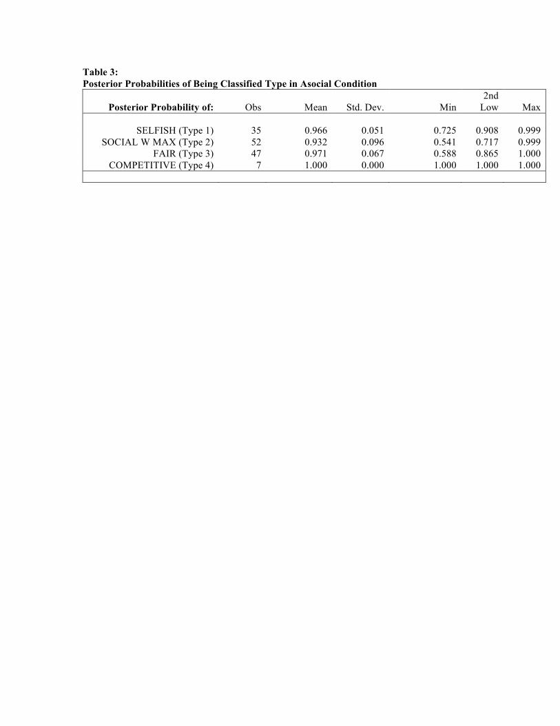
Table 3: Posterior Probabilities of Being Classified Type in Asocial Condition

Posterior Probability of: Obs Mean Std. Dev. Min 2nd

Low Max

SELFISH (Type 1) 35 0.966 0.051 0.725 0.908 0.999 SOCIAL W MAX (Type 2) 52 0.932 0.096 0.541 0.717 0.999

FAIR (Type 3) 47 0.971 0.067 0.588 0.865 1.000 COMPETITIVE (Type 4) 7 1.000 0.000 1.000 1.000 1.000

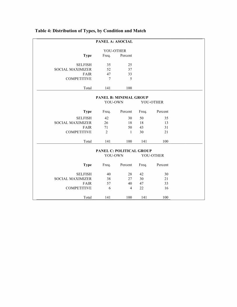
Table 4: Distribution of Types, by Condition and Match

PANEL A: ASOCIAL

YOU-OTHER Type Freq. Percent

SELFISH 35 25 SOCIAL MAXIMIZER 52 37

FAIR 47 33 COMPETITIVE 7 5

Total 141 100

PANEL B: MINIMAL GROUP

YOU-OWN YOU-OTHER

Type Freq. Percent Freq. Percent

SELFISH 42 30 50 35 SOCIAL MAXIMIZER 26 18 18 13

FAIR 71 50 43 31 COMPETITIVE 2 1 30 21

Total 141 100 141 100

PANEL C: POLITICAL GROUP

YOU-OWN YOU-OTHER

Type Freq. Percent Freq. Percent

SELFISH 40 28 42 30 SOCIAL MAXIMIZER 38 27 30 21

FAIR 57 40 47 33 COMPETITIVE 6 4 22 16

Total 141 100 141 100

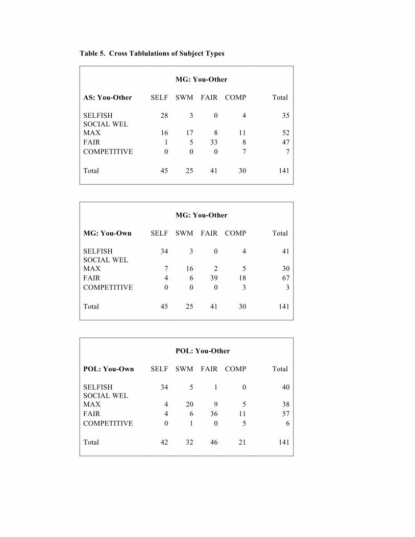
Table 5. Cross Tablulations of Subject Types

MG: You-Other

AS: You-Other SELF SWM FAIR COMP Total

SELFISH 28 3 0 4 35 SOCIAL WEL MAX 16 17 8 11 52 FAIR 1 5 33 8 47 COMPETITIVE 0 0 0 7 7

Total 45 25 41 30 141

MG: You-Other

MG: You-Own SELF SWM FAIR COMP Total


Total 45 25 41 30 141

POL: You-Other

POL: You-Own SELF SWM FAIR COMP Total


Total 42 32 46 21 141

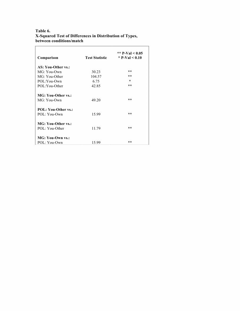
Table 6. X-Squared Test of Differences in Distribution of Types, between conditions/match

Comparison Test Statistic

** P-Val < 0.05 * P-Val < 0.10

AS: You-Other vs.: MG: You-Own 30.23 **

MG: You-Other 104.57 ** POL:You-Own 6.75 * POL:You-Other 42.85 **

MG: You-Other vs.: MG: You-Own 49.20 **

POL: You-Other vs.:

POL: You-Own 15.99 **

MG: You-Other vs.: POL: You-Other 11.79 **

MG: You-Own vs.:

POL: You-Own 15.99 **

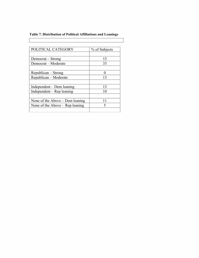
Table 7. Distribution of Political Affiliations and Leanings

POLITICAL CATEGORY % of Subjects Democrat – Strong 15 Democrat – Moderate 33 Republican – Strong 0 Republican – Moderate 13 Independent – Dem leaning 13 Independent – Rep leaning 10 None of the Above – Dem leaning 11 None of the Above - Rep leaning 5

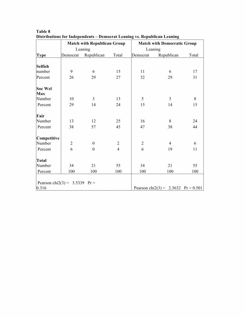
Table 8 Distributions for Independents – Democrat Leaning vs. Republican Leaning

Match with Republican Group Match with Democratic Group Leaning Leaning Type Democrat Republican Total Democrat Republican Total

Selfish number 9 6 15 11 6 17 Percent 26 29 27 32 29 31

Soc Wel Max Number 10 3 13 5 3 8 Percent 29 14 24 15 14 15

Fair Number 13 12 25 16 8 24 Percent 38 57 45 47 38 44

Competitive Number 2 0 2 2 4 6 Percent 6 0 4 6 19 11

Total Number 34 21 55 34 21 55 Percent 100 100 100 100 100 100

Pearson chi2(3) = 3.5339 Pr = 0.316 Pearson chi2(3) = 2.3632 Pr = 0.501

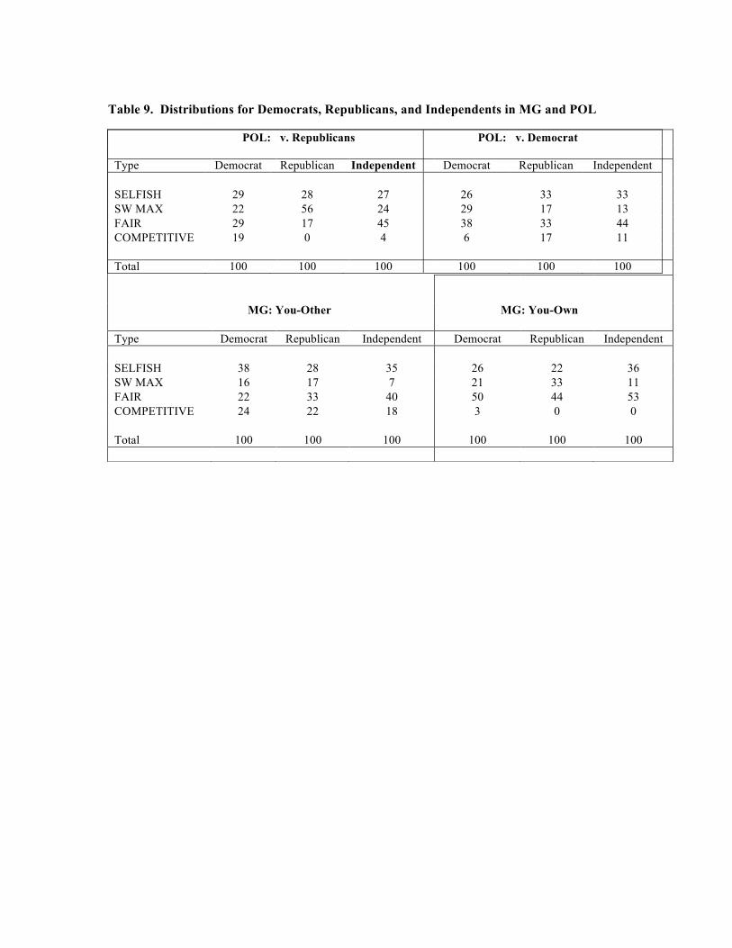
Table 9. Distributions for Democrats, Republicans, and Independents in MG and POL

MG: You-Other

MG: You-Own

Type Democrat Republican Independent Democrat Republican Independent SELFISH 38 28 35 26 22 36 SW MAX 16 17 7 21 33 11 FAIR 22 33 40 50 44 53 COMPETITIVE 24 22 18 3 0 0

Total 100 100 100 100 100 100

POL: v. Republicans POL: v. Democrat

Type Democrat Republican Independent Democrat Republican Independent SELFISH 29 28 27 26 33 33 SW MAX 22 56 24 29 17 13 FAIR 29 17 45 38 33 44 COMPETITIVE 19 0 4 6 17 11

Total 100 100 100 100 100 100

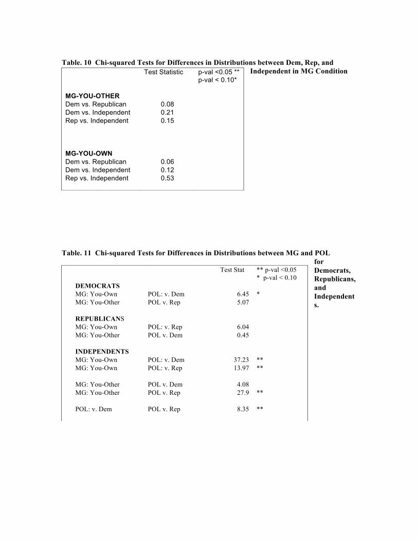
Table. 10 Chi-squared Tests for Differences in Distributions between Dem, Rep, and

Independent in MG Condition

Table. 11 Chi-squared Tests for Differences in Distributions between MG and POL

for Democrats, Republicans, and Independents.

Test Statistic p-val <0.05 **

p-val < 0.10* MG-YOU-OTHER

Dem vs. Republican 0.08 Dem vs. Independent 0.21 Rep vs. Independent 0.15

MG-YOU-OWN

Dem vs. Republican 0.06 Dem vs. Independent 0.12 Rep vs. Independent 0.53

Test Stat ** p-val <0.05

* p-val < 0.10

DEMOCRATS

MG: You-Own POL: v. Dem 6.45 *

MG: You-Other POL v. Rep 5.07

REPUBLICANS

MG: You-Own POL: v. Rep 6.04

MG: You-Other POL v. Dem 0.45

INDEPENDENTS

MG: You-Own POL: v. Dem 37.23 **

MG: You-Own POL: v. Rep 13.97 **

MG: You-Other POL v. Dem 4.08

MG: You-Other POL v. Rep 27.9 **

POL: v. Dem POL v. Rep 8.35 **

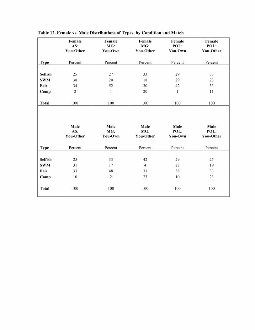
Table 12. Female vs. Male Distributions of Types, by Condition and Match

Female Female Female Female Female

AS: You-Other

MG: You-Own

MG: You-Other

POL: You-Own

POL: You-Other

Type Percent Percent Percent Percent Percent Selfish 25 27 33 29 33 SWM 38 20 18 29 23 Fair 34 52 30 42 33 Comp 2 1 20 1 11

Total 100 100 100 100 100

Male Male Male Male Male

AS: You-Other

MG: You-Own

MG: You-Other

POL: You-Own

POL: You-Other


Total 100 100 100 100 100

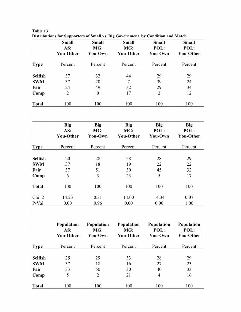
Table 13 Distributions for Supporters of Small vs. Big Government, by Condition and Match

Small Small Small Small Small

AS: You-Other

MG: You-Own

MG: You-Other

POL: You-Own

POL: You-Other


Total 100 100 100 100 100

Big Big Big Big Big

AS: You-Other

MG: You-Own

MG: You-Other

POL: You-Own

POL: You-Other


Total 100 100 100 100 100

Chi_2 14.23 0.31 14.00 14.34 0.07 P-Val 0.00 0.96 0.00 0.00 1.00

Population Population Population Population Population

AS: You-Other

MG: You-Own

MG: You-Other

POL: You-Own

POL: You-Other


Total 100 100 100 100 100

Appendix Below is the instruction sheet presented to each participant. PAGE 1 WELCOME! INSTRUCTIONS Thank you for participating in this experiment. The object of this investigation is to study how people make decisions. There is no deception in this experiment – and we want you to understand everything about the procedures. If you have any questions at any time, please ask the experiment organizer in the room. PART I: THE CHOICE TASK A) During the experiment, you will be presented with a series of choices. For each choice, you will be asked to award points to between either (1) yourself and another participant or (2) two other participants. You will earn the points you allocate to yourself, and the other person will earn the points you allocate to him or her. At the end of the experiment, one of your choices will be selected at random by a computer and the points earned will be converted into payments. Each decision is independent from the others. Your decisions and outcomes in one choice will not affect your outcomes in any other choice. For each choice, you will be paired with new participants. Use LEFT and RIGHT arrow keys to make your choices. PART II and III: A) INITIAL SURVEY You will take a brief survey. There are no right or wrong answers. Your answers to these questions will not affect your payments. Please only use the RIGHT and LEFT arrow keys or NUMBER keys as instructed to answer all questions. B) THE CHOICE TASK After completing the initial survey, you will once again be presented with a series of choices. You will be anonymously paired with two new participants. These participants will remain the same throughout this part of the experiment. At the end of the experiment, one of your choices will be selected at random by a computer and the points earned will be converted into payments. Each decision is independent from the others. Your decisions and outcomes in one choice will not affect your outcomes in any other choice. TURN PAGE OVER FOR ADDITIONAL INSTRUCTIONS

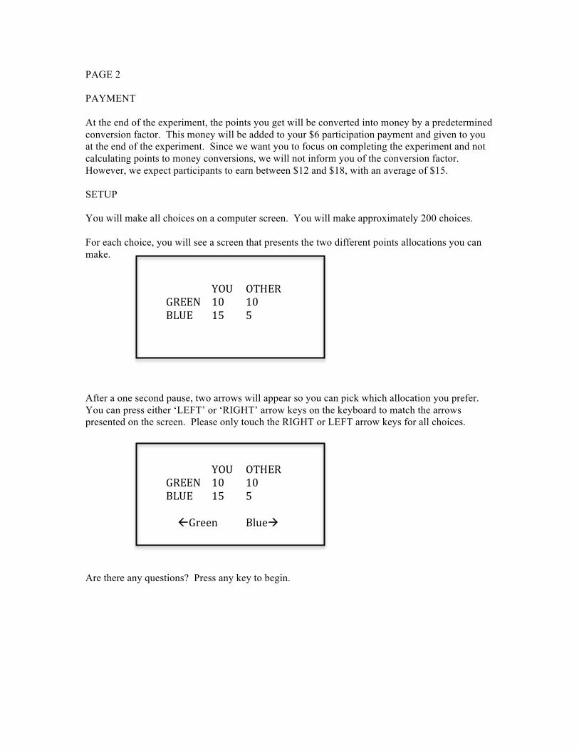
PAYMENT At the end of the experiment, the points you get will be converted into money by a predetermined conversion factor. This money will be added to your $6 participation payment and given to you at the end of the experiment. Since we want you to focus on completing the experiment and not calculating points to money conversions, we will not inform you of the conversion factor. However, we expect participants to earn between $12 and $18, with an average of $15. SETUP You will make all choices on a computer screen. You will make approximately 200 choices. For each choice, you will see a screen that presents the two different points allocations you can make. After a one second pause, two arrows will appear so you can pick which allocation you prefer. You can press either ‘LEFT’ or ‘RIGHT’ arrow keys on the keyboard to match the arrows presented on the screen. Please only touch the RIGHT or LEFT arrow keys for all choices. Are there any questions? Press any key to begin.

YOU OTHER GREEN 10 10 BLUE 15 5

YOU OTHER GREEN 10 10 BLUE 15 5

ßGreen Blueà

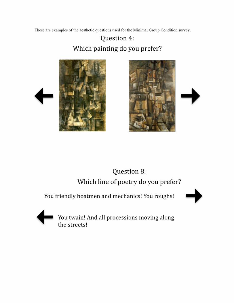
These are examples of the aesthetic questions used for the Minimal Group Condition survey.

Question 4: Which painting do you prefer?

You friendly boatmen and mechanics! You roughs!

You twain! And all processions moving along the streets!

Question 8: Which line of poetry do you prefer?

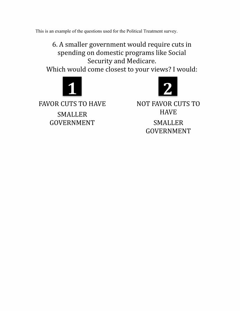
This is an example of the questions used for the Political Treatment survey.

6. A smaller government would require cuts in spending on domestic programs like Social

Security and Medicare. Which would come closest to your views? I would:

FAVOR CUTS TO HAVE

SMALLER GOVERNMENT

NOT FAVOR CUTS TO HAVE

SMALLER GOVERNMENT

1 2

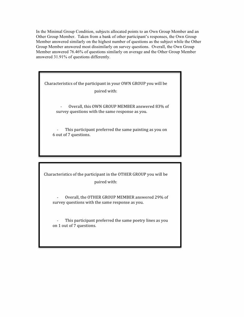
In the Minimal Group Condition, subjects allocated points to an Own Group Member and an Other Group Member. Taken from a bank of other participant’s responses, the Own Group Member answered similarly on the highest number of questions as the subject while the Other Group Member answered most dissimilarly on survey questions. Overall, the Own Group Member answered 76.46% of questions similarly on average and the Other Group Member answered 31.91% of questions differently.

Characteristics of the participant in your OWN GROUP you will be paired with:

- Overall, this OWN GROUP MEMBER answered 83% of survey questions with the same response as you.

- This participant preferred the same painting as you on 6 out of 7 questions.

Characteristics of the participant in the OTHER GROUP you will be paired with:

- Overall, the OTHER GROUP MEMBER answered 29% of survey questions with the same response as you.

- This participant preferred the same poetry lines as you on 1 out of 7 questions.

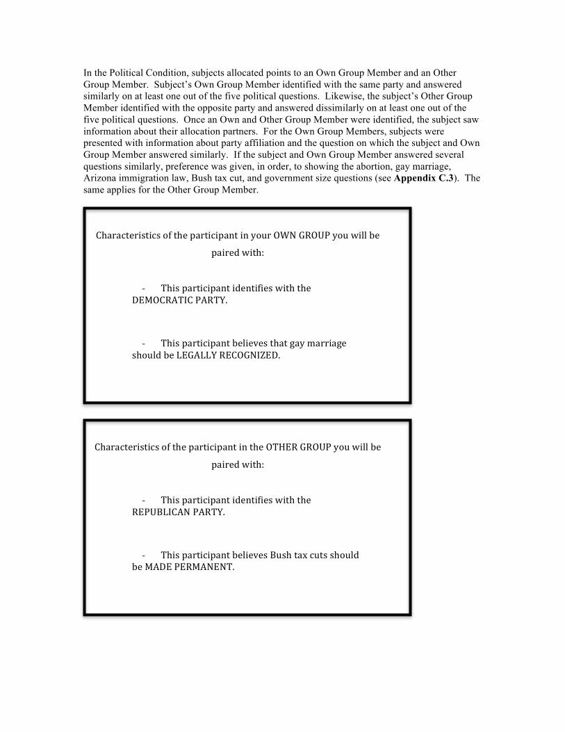
In the Political Condition, subjects allocated points to an Own Group Member and an Other Group Member. Subject’s Own Group Member identified with the same party and answered similarly on at least one out of the five political questions. Likewise, the subject’s Other Group Member identified with the opposite party and answered dissimilarly on at least one out of the five political questions. Once an Own and Other Group Member were identified, the subject saw information about their allocation partners. For the Own Group Members, subjects were presented with information about party affiliation and the question on which the subject and Own Group Member answered similarly. If the subject and Own Group Member answered several questions similarly, preference was given, in order, to showing the abortion, gay marriage, Arizona immigration law, Bush tax cut, and government size questions (see Appendix C.3). The same applies for the Other Group Member.

- This participant identifies with the DEMOCRATIC PARTY.

Characteristics of the participant in your OWN GROUP you will be paired with:

- This participant believes that gay marriage should be LEGALLY RECOGNIZED.

- This participant identifies with the REPUBLICAN PARTY.

Characteristics of the participant in the OTHER GROUP you will be paired with:

- This participant believes Bush tax cuts should be MADE PERMANENT.

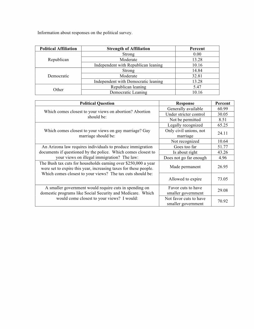
Information about responses on the political survey.

Political Affiliation Strength of Affiliation Percent

Republican Strong 0.00

Moderate 13.28 Independent with Republican leaning 10.16

Democratic Strong 14.84

Moderate 32.81 Independent with Democratic leaning 13.28

Other Republican leaning 5.47 Democratic Leaning 10.16

Political Question Response Percent

Which comes closest to your views on abortion? Abortion should be:

Generally available 60.99 Under stricter control 30.05

Not be permitted 8.51

Which comes closest to your views on gay marriage? Gay marriage should be:

Legally recognized 65.25 Only civil unions, not

marriage 24.11

Not recognized 10.64 An Arizona law requires individuals to produce immigration

documents if questioned by the police. Which comes closest to your views on illegal immigration? The law:

Goes too far 51.77 Is about right 43.26

Does not go far enough 4.96 The Bush tax cuts for households earning over $250,000 a year were set to expire this year, increasing taxes for these people. Which comes closest to your views? The tax cuts should be:

Made permanent 26.95

Allowed to expire 73.05

A smaller government would require cuts in spending on domestic programs like Social Security and Medicare. Which

would come closest to your views? I would:

Favor cuts to have smaller government 29.08

Not favor cuts to have smaller government 70.92

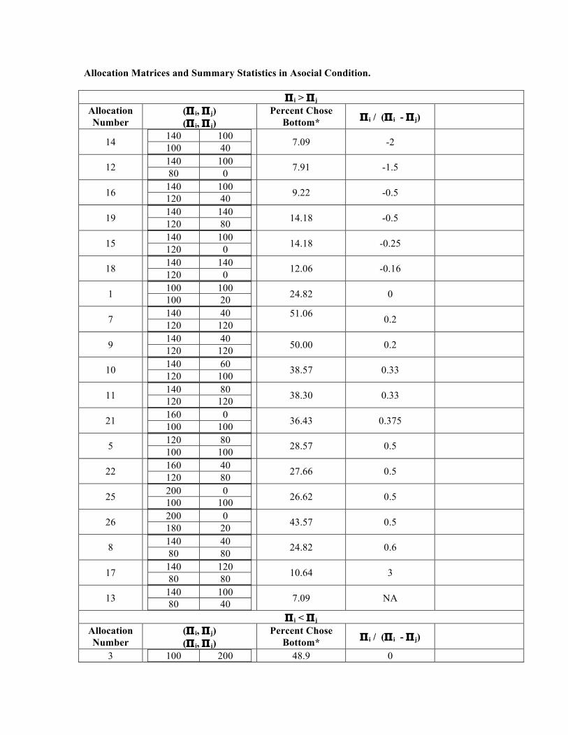
Allocation Matrices and Summary Statistics in Asocial Condition.

Π i > Π j Allocation Number

(Π i, Π j) (Π i, Π j)

Percent Chose Bottom* Π i / (Π i - Π j)

14 140 100 100 40

7.09 -2

12 140 100 80 0

7.91 -1.5

16 140 100 120 40

9.22 -0.5

19 140 140 120 80

14.18 -0.5

15 140 100 120 0

14.18 -0.25

18 140 140 120 0

12.06 -0.16

1 100 100 100 20

24.82 0

7 140 40 120 120

51.06 0.2

9 140 40 120 120

50.00 0.2

10 140 60 120 100

38.57 0.33

11 140 80 120 120

38.30 0.33

21 160 0 100 100

36.43 0.375

5 120 80 100 100

28.57 0.5

22 160 40 120 80

27.66 0.5

25 200 0 100 100

26.62 0.5

26 200 0 180 20

43.57 0.5

8 140 40 80 80

24.82 0.6

17 140 120 80 80

10.64 3

13 140 100 80 40

7.09 NA

Π i < Π j Allocation Number

(Π i, Π j) (Π i, Π j)

Percent Chose Bottom* Π i / (Π i - Π j)

3 100 200 48.9 0

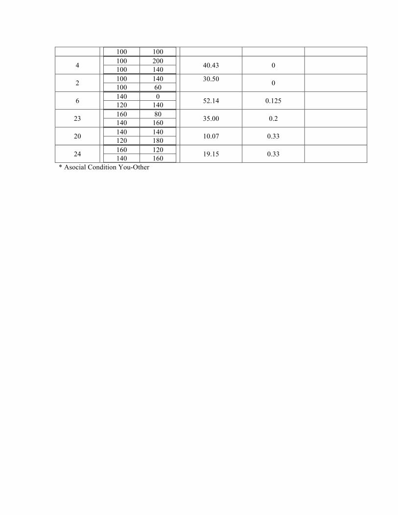
100 100

4 100 200 100 140

40.43 0

2 100 140 100 60

30.50 0

6 140 0 120 140

52.14 0.125

23 160 80 140 160

35.00 0.2

20 140 140 120 180

10.07 0.33

24 160 120 140 160

19.15 0.33

* Asocial Condition You-Other

identity, group conflict, and social preferences

Documents