identification of systems in terms of the wiener · pdf fileitself as a basis for system...
TRANSCRIPT
1
Technical Note 1967-34
Identification of Systems in Terms of the Wiener Model
C. R. Arnold
22 Aug> >67
Lincoln Laboratory

•
The work reported in this document was performed at Lincoln Laboratory, a center for research/operated: by Massachusetts Institute of Technology, with the support of the U.S. Air Force under Contract AF 19 (628)-5167.
This report may be reproduced to satisfy needs of U.S. Government agencies.
This document has been approved for public release and sale; its distribution is unlimited.
MASSACHUSETTS INSTITUTE OF TECHNOLOGY
LINCOLN LABORATORY
IDENTIFICATION OF SYSTEMS
IN TERMS OF THE WIENER MODEL
C. R. ARNOLD
Group 22
TECHNICAL NOTE 1967-34
22 AUGUST 1967
LEXINGTON MASSACHUSETTS
ABSTRACT
This report presents briefly a nonlinear model originally proposed
by the late Norbert Wiener for the characterization of general
systems. Three procedures are then offered for the identification
of any given system in terms of the Wiener model. Finally, this
report presents the results of a digital computer simulation study
(utilizing six somewhat arbitrary systems) which was designed to
evaluate the various identification procedures as well as the model
itself as a basis for system identification.
Accepted for the Air Force Franklin C. Hudson Chief, Lincoln Laboratory Office
111
PREFACE
The research reported in this report was conducted during the
spring and summer of 1965 while the author was a part-time
student at Harvard University under the direction of Professor
K. S. Narendra (presently at Yale University). It was presented
by Professor Narendra at the Third Annual Allerton Conference
on Circuit and System Theory (October 1965) under the title,
"On the Use of the Wiener Model for Identification in Adaptive
Situations."
The author takes pleasure to acknowledge Lincoln Laboratory
for its support in this research. It is also a pleasure to
acknowledge Harvard University and Professor Narendra for
the intellectual benefits received by virtue of this association.
Finally, I wish to thank my former colleague Dr. Harold K.
Knudsen and fellow-student Charles P. Neuman for their
patient listening and many helpful discussions.
IV
TABLE OF CONTENTS
I. INTRODUCTION 1
II. THE WIENER MODEL 3
IU. IDENTIFICATION PROCEDURES 7
IV. THE UNKNOWN SYSTEMS 13
V. RESULTS FROM THE COMPUTER SIMULATION 16
VI. SUMMARY AND CONCLUSIONS 43
REFERENCES 45
I. INTRODUCTION
The problem of system identification may be formulated somewhat ab-
stractly as:
Given some physical system S and a class C of system models, the
identification problem is to determine that specific model M in C
which is equivalent (in some sense) to S. The identification is to be
accomplished through the observation, often in the presence of noise,
of the response of S to various probe functions.
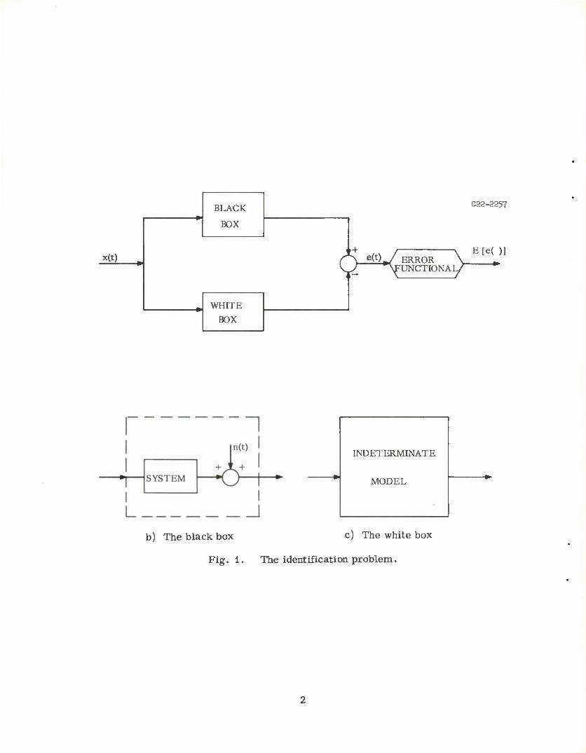
The identification problem may be represented schematically as in Fig. 1
where the black box represents the unknown physical system with, in general, a
noisy output. The white box represents an indeterminate model from some class.
The problem being to specialize the white box so that the resulting model is equi-
valent to the black box. The equivalence being in terms of the satisfaction of some
criterion by some functional of the error between the system and model for some
class of inputs.
In practice the engineer usually chooses, and rightly so, some class of
linear models for his white box. Then, he is usually able to determine an adequate
model from within some class of models - maybe not his original choice but at
least a linear class - and all is well. However, there are times when no linear
model can be found which will meet one' s adequacy criterion. Then one is forced
to consider the identification of systems in terms of nonlinear models.
As to possible nonlinear models, numerous ones have been proposed over
the years and they are surveyed in the author's report [1]. One such nonlinear
model for the characterization of general systems was proposed by Norbert
Wiener [2] in 1949. After a very brief description of the Wiener model in the next
section, this report goes on to describe a simulation study (on the IBM-7094 digital
computer) which was designed to evaluate the Wiener model as a basis for the iden-
tification of real physical systems. As far as this author knows, there has been no attempts to date to actually implement the Wiener model.
x(t)
BLACK
BOX
WHITE
BOX
o- e(t). ERROR \ FUNCTIONAL/
C22-2257
E[e( )]
INDETERMINATE
MODEL
b) The black box c) The white box
Fig. 1. The identification problem.
II. THE WIENER MODEL
In 1949 Wiener [2] specialized an orthogonal functional decomposition
technique of Cameron and Martin [3] to obtain a general model for nonlinear
systems. Specifically, as a basis for the generalized Fourier decomposition of
[3] , Wiener chose the Laguerre functions [4] which are most appropriate for the
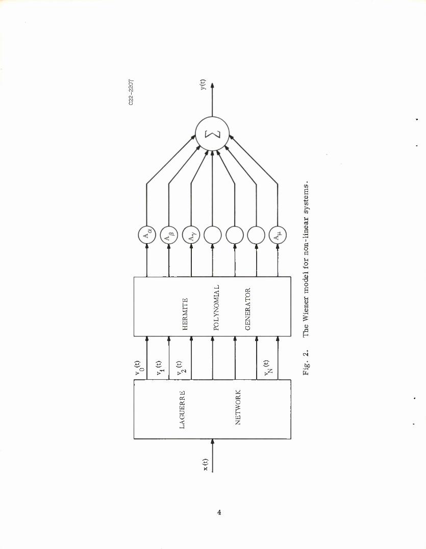
modeling of physical realizable systems. The resulting model is given schematically
in Fig. 2.
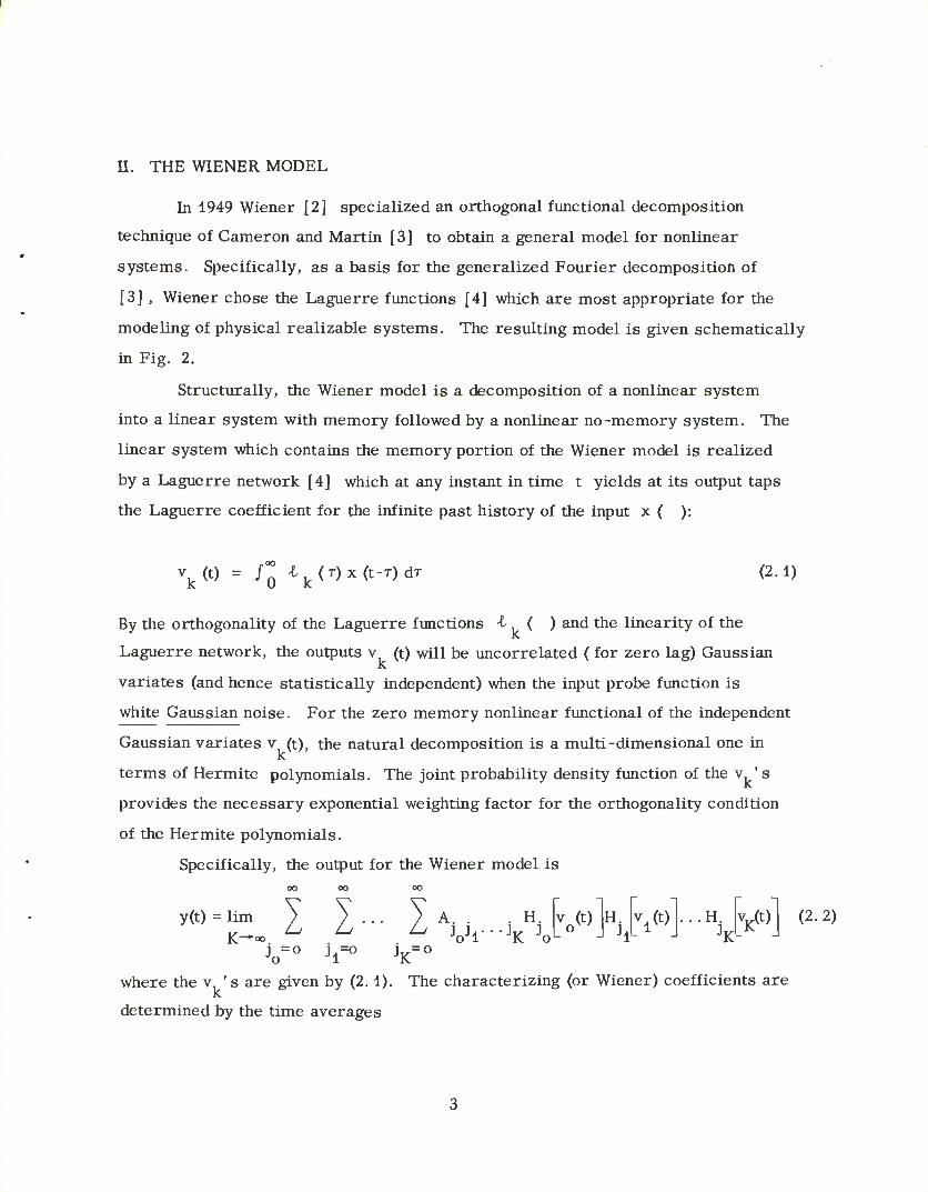
Structurally, the Wiener model is a decomposition of a nonlinear system
into a linear system with memory followed by a nonlinear no-memory system. The
linear system which contains the memory portion of the Wiener model is realized
by a Laguerre network [4] which at any instant in time t yields at its output taps
the Laguerre coefficient for the infinite past history of the input x ( ):
\(t) = /0 *k(T)X(t-T)dT (2.1)
By the orthogonality of the Laguerre functions •£, ( ) and the linearity of the
Laguerre network, the outputs v (t) will be uncorrelated ( for zero lag) Gaussian
variates (and hence statistically independent) when the input probe function is
white Gaussian noise. For the zero memory nonlinear functional of the independent
Gaussian variates v (t), the natural decomposition is a multi-dimensional one in
terms of Hermite polynomials. The joint probability density function of the v ' s
provides the necessary exponential weighting factor for the orthogonality condition
of the Hermite polynomials.
Specifically, the output for the Wiener model is
y(t) = lim K
m > ) ... ) A. H.
jo=° jl=° jK=°
vjt) H. Jl
- —
v^t) ...H. vK(t) (2.2)
where the v, 's are given by (2. 1). The characterizing (or Wiener) coefficients are
determined by the time averages
o CM C\J
I CM OJ o
3 PS o
w ^ H H p < >—i Pi w Pi J Z w 2 w X o
^^» v•^ >—V 4-» •*-» •M 4->
o > 7^ T^ >2
w w Pd Pi oi o w <<£ D [-1
o UJ -< 2 J
1 1
^~* 4-t
X
a CD *-> CO
H a
o a u o
-8 o a M 0) a 0)
CD
CN
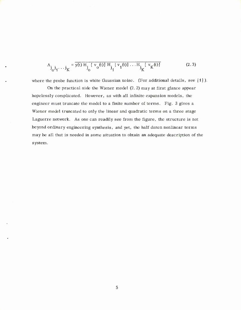
i =y(t)H [v (t)] H [v (t)]...H [v JoJl---JK Jo ° h 1 JK K
(t)] (2.3)
where the probe function is white Gaussian noise. (For additional details, see [1] ).
On the practical side the Wiener model (2. 2) may at first glance appear
hopelessly complicated. However, as with all infinite expansion models, the
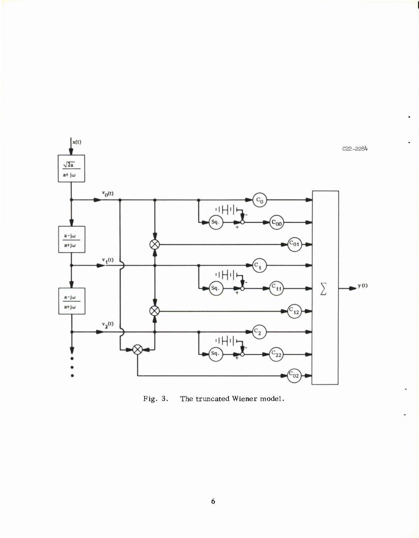
engineer must truncate the model to a finite number of terms. Fig. 3 gives a
Wiener model truncated to only the linear and quadratic terms on a three stage
Laguerre network. As one can readily see from the figure, the structure is not
beyond ordinary engineering synthesis, and yet, the half dozen nonlinear terms
may be all that is needed in some situation to obtain an adequate description of the
system.
C22-22814-
Fig. 3. The truncated Wiener model.
III. IDENTIFICATION PROCEDURES
A. The Direct Method
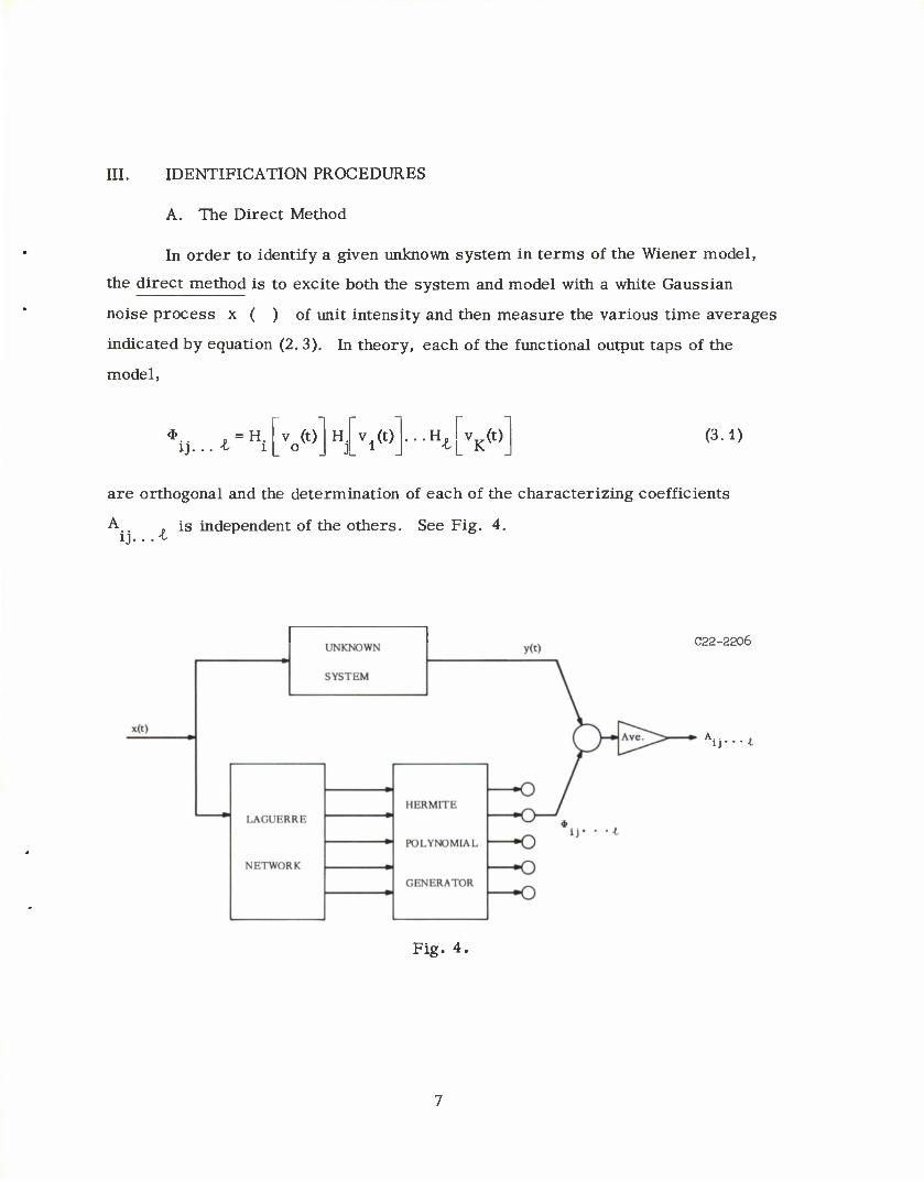
In order to identify a given unknown system in terms of the Wiener model,
the direct method is to excite both the system and model with a white Gaussian
noise process x ( ) of unit intensity and then measure the various time averages
indicated by equation (2. 3). In theory, each of the functional output taps of the
model,
4> ij-
. =H. I l
vjt) H v4(t) ...HJLvK(t) (3.1)
are orthogonal and the determination of each of the characterizing coefficients
A.. .is independent of the others. See Fig. 4. 1J...-C
C22-2206
Fig. 4.
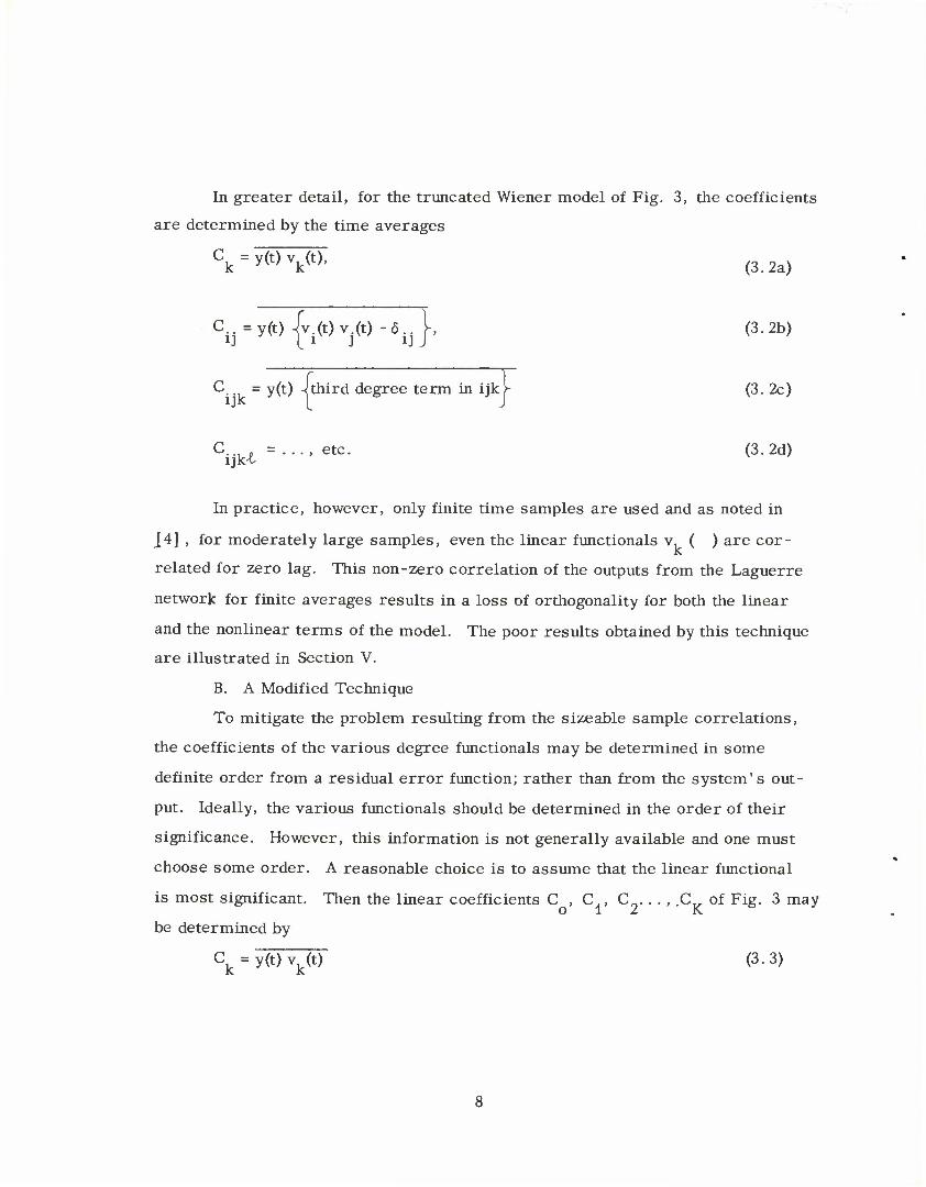
In greater detail, for the truncated Wiener model of Fig. 3, the coefficients
are determined by the time averages
Ck = ^ Vk(t)' (3.2a)
Cij=y(t) (vi^vj(t) "6ij}' (3-2b>
^- i. = y(t) Xthird degree term in ijk V (3. 2c)
C.jU .....etc. (3. 2d)
In practice, however, only finite time samples are used and as noted in
[4] , for moderately large samples, even the linear functionals v, ( ) are cor-
related for zero lag. This non-zero correlation of the outputs from the Laguerre
network for finite averages results in a loss of orthogonality for both the linear
and the nonlinear terms of the model. The poor results obtained by this technique
are illustrated in Section V.
B. A Modified Technique
To mitigate the problem resulting from the sizeable sample correlations,
the coefficients of the various degree functionals may be determined in some
definite order from a residual error function; rather than from the system's out-
put. Ideally, the various functionals should be determined in the order of their
significance. However, this information is not generally available and one must
choose some order. A reasonable choice is to assume that the linear functional
is most significant. Then the linear coefficients C , C , C . . . , .C of Fig. 3 may
be determined by
Ck = y(t)vk(t) (3.3)
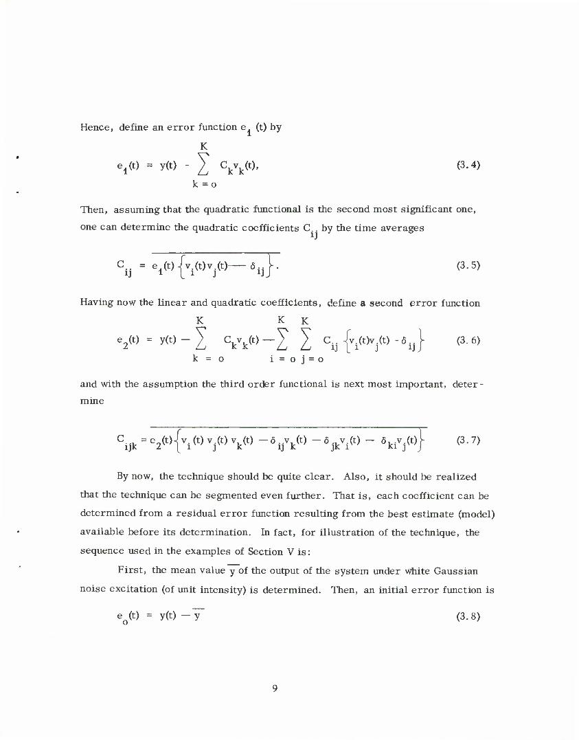
Hence, define an error function e (t) by
e4(t) = y(t) - 2_, CkVk(t)' <3'4>
k = o
Then, assuming that the quadratic functional is the second most significant one,
one can determine the quadratic coefficients C.. by the time averages
\ = e4(t) (v.(t)v.(t) a^J. (3.5)
Having now the linear and quadratic coefficients, define a second error function
K K K
k=o i=oj=o e2(t) = y<t>-£ VkW-Z I C« {'iWj* •* J <3'
and with the assumption the third order functional is next most important, deter-
mine
cijk=e2(t>{vi(t)vj<t)vk(t' -Vk(t) "W" - \ivM <37>
By now, the technique should be quite clear. Also, it should be realized
that the technique can be segmented even further. That is, each coefficient can be
determined from a residual error function resulting from the best estimate (model)
available before its determination. In fact, for illustration of the technique, the
sequence used in the examples of Section V is:
First, the mean value y of the output of the system under white Gaussian
noise excitation (of unit intensity) is determined. Then, an initial error function is
eQ(t) = y(t) -y~ (3.8)
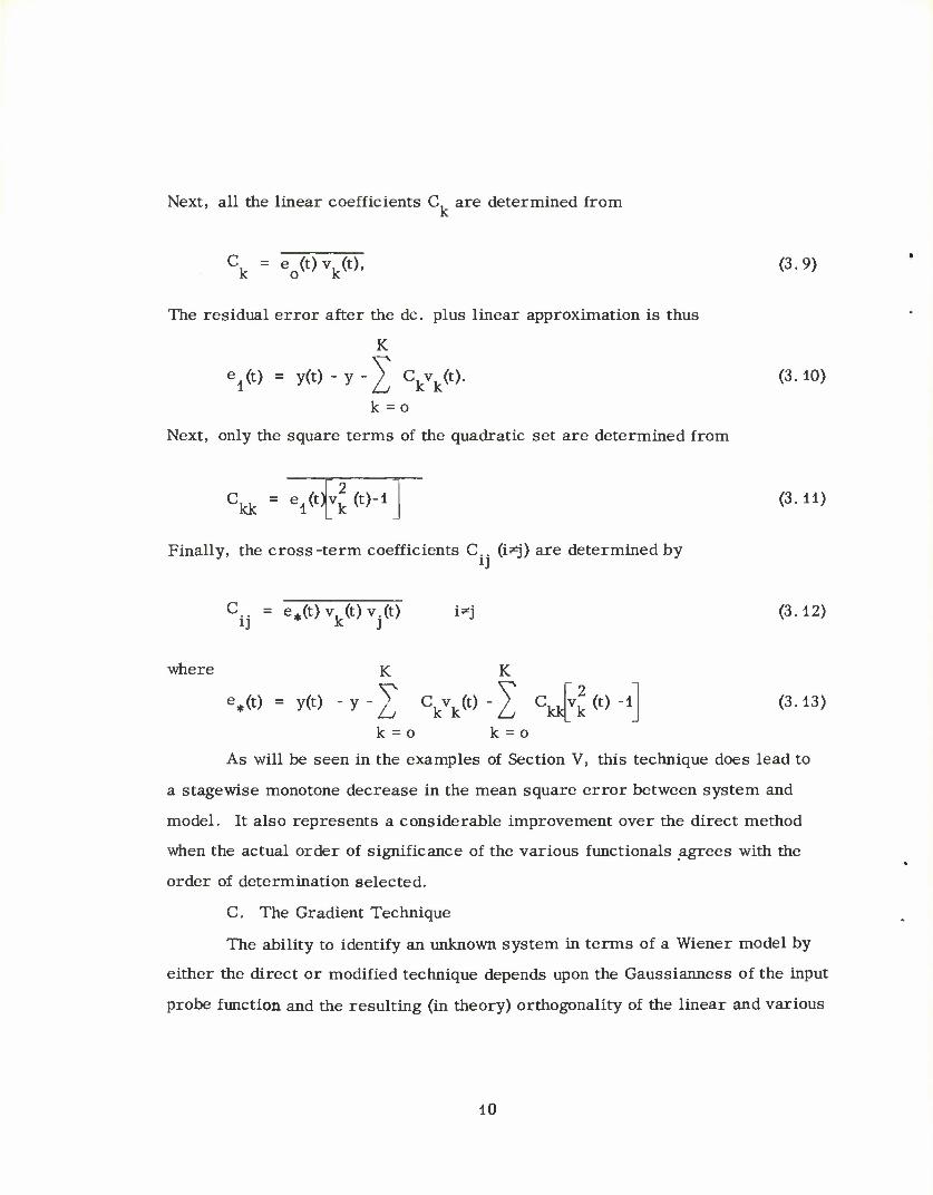
Next, all the linear coefficients C, are determined from
Ck - ao(t,vt(t,, (3.9)
The residual error after the dc. plus linear approximation is thus
K
V>-iW-y-^Vk* k = o
Next, only the square terms of the quadratic set are determined from
Ckk " 6l(t^ (t)-4
Finally, the cross-term coefficients C. (i^) are determined by
(3.10)
(3.H)
Cij = e*<0 vk(t) v (t) {*i (3.12)
where K
%(t) = y(t) -y-V ck vi>-I v. (t) -1 kk k (3.13)
k = o k = o
As will be seen in the examples of Section V, this technique does lead to
a stagewise monotone decrease in the mean square error between system and
model. It also represents a considerable improvement over the direct method
when the actual order of significance of the various functionals agrees with the
order of determination selected.
C. The Gradient Technique
The ability to identify an unknown system in terms of a Wiener model by
either the direct or modified technique depends upon the Gaussianness of the input
probe function and the resulting (in theory) orthogonality of the linear and various
10
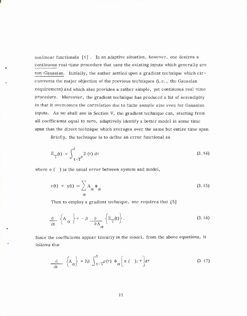
nonlinear functionals [1] . In an adaptive situation, however, one desires a
continuous real-time procedure that uses the existing inputs which generally are
non-Gaussian. Initially, the author settled upon a gradient technique which cir-
cumvents the major objection of the previous techniques (i.e. , the Gaussian
requirement) and which also provides a rather simple, yet continuous real-time
procedure. Moreover, the gradient technique has produced a bit of serendipity
in that it overcomes the correlation due to finite sample size even for Gaussian
inputs. As we shall see in Section V, the gradient technique can, starting from
all coefficients equal to zero, adaptively identify a better model in some time
span than the direct technique which averages over the same but entire time span.
Briefly, the technique is to define an error functional as
E (t) = f 2(r)dr (3.14) t-T
where e ( ) is the usual error between system and model,
e(t) = y(t) -YA $ (3.15) L-i a a a
Then to employ a gradient technique, one requires that [5]
d A V= -/? d iE(t)V. (3.16) lla[ "8A" I T J
a
Since the coefficients appear linearly in the model, from the above equations, it
follows thar
•fA,[=2MfTe(T)*a dt *- f, x( ); T dT (3. 17)
11
By formally integrating (3. 17), one has
,t ~t
o L-
d4d (3.18)
If one adjusts the coefficients A in a continuous fashion as indicated by (3.18), a
the error functional (3.14) for a time-invariant system will be minimized and
the final value A (oo) will yield the required characterizing coefficients. In an
adaptive situation for a stochastically time-varying system, (3.18) can be imple-
mented on a digital computer by
A (n+l) = A (n)-£z (n + 1) (3.19) a a. a.
where the correction z (n + 1) is equivalent to the inner integral of (3. 18) and
may be implemented by a driving simple low-pass (recursive) digital filter with
the product of the error and the specific functional * , e.g.
z (n + 1) = Az (n) + /ie(n + 1) * a a a
n+1 (3. 20)
for some A., JI. For X almost equal to one, the time constant of the low pass
filter is quite long and effectively evaluates the integral in (3.18). The choice
of n can be absorbed into the choice of /3 which does offer some problem. Ideally,
initially /3 should be large for rapid convergence but as the minimum is approached,
one would like a smaller /? just to hold one's solution. However, the author has
worked only with a fixed /? who's selection has required at most three attempts.
12
IV. THE UNKNOWN SYSTEMS
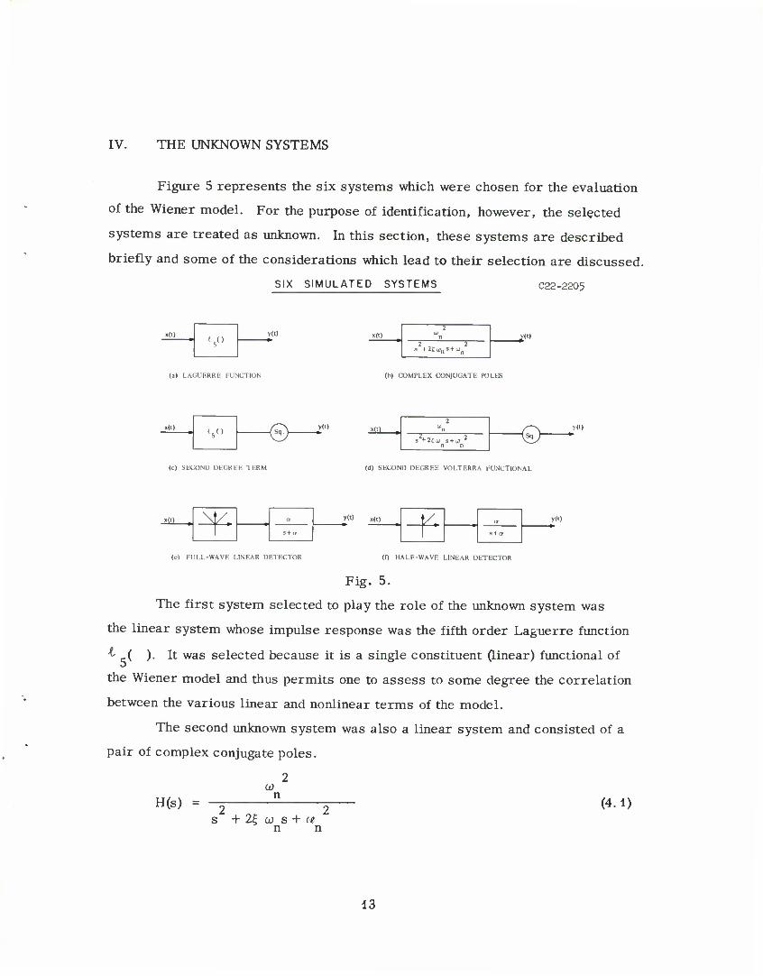
Figure 5 represents the six systems which were chosen for the evaluation
of the Wiener model. For the purpose of identification, however, the selected
systems are treated as unknown. In this section, these systems are described
briefly and some of the considerations which lead to their selection are discussed.
SIX SIMULATED SYSTEMS C22-2205
v> y(t)
(a) l.AGUERRE FUNCTION
s +2£w s+o
(b) COMPLEX CONJUGATE POLES
»(0
(c) SECOND DECREE TERM
v(l) _x(j]_
s +2£u s+u 2
n n <£y (d) SECOND DEGREE VOLTERRA FUNCTIONAL
yft)
»<•)
(c) FULL-WAVE LINEAR DETECTOR
y(') x(t) v(l)
(0 HALF-WAVE LINEAR DETECTOR
Fig. 5.
The first system selected to play the role of the unknown system was
the linear system whose impulse response was the fifth order Laguerre function
t A ). It was selected because it is a single constituent (linear) functional of
the Wiener model and thus permits one to assess to some degree the correlation
between the various linear and nonlinear terms of the model.
The second unknown system was also a linear system and consisted of a
pair of complex conjugate poles.
2 u)
H(s) = n
2 2 s + 2| u> s + «
n n
(4.1)
13
The damping ratio £ was taken to be 0.1 and hence (4.1) represents a rather
narrow band system. This is the same system considered in [4] and its further
consideration here is justified in that it provides a non-trivial approximation
problem for the Laguerre functions for even a linear model.
The third system consisted of an isolated second degree term of the
Wiener model. Namely, the linear system with impulse response -t ( ) fol-
lowed by a square-law device. Its choice was also motivated (as in the case of
the first system) by a desire to assess the correlation between the various linear
and nonlinear terms of the model.
The fourth unknown system consisted of the second system above followed
by a square-law device. It represents an isolated second degree Volterra
functional [1] whose Wiener coefficients may be calculated exactly with some
effort. As will be seen in the next section, however, it affords a rather difficult
system for approximation by the Wiener model.
The last two selected systems were the full-wave and half-wave linear
detectors. They provide non-trivial systems for approximation by the Wiener
model in that the first (full-wave) contains Volterra functions of all even order
(0, 2, 4, ...) and the latter (half-wave) contains functionals of all order in its
repres entation.
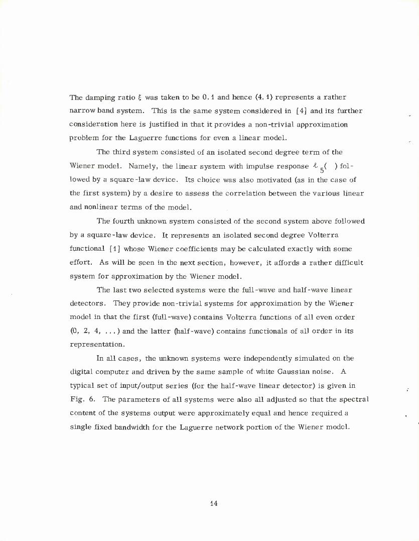
In all cases, the unknown systems were independently simulated on the
digital computer and driven by the same sample of white Gaussian noise. A
typical set of input/output series (for the half-wave linear detector) is given in
Fig. 6. The parameters of all systems were also all adjusted so that the spectral
content of the systems output were approximately equal and hence required a
single fixed bandwidth for the Laguerre network portion of the Wiener model.
14
o C\J
CM i
OJ
o
U O «-! o 0) •1-1
•s H 03
J2
n o
3 a
I SO
OH
15
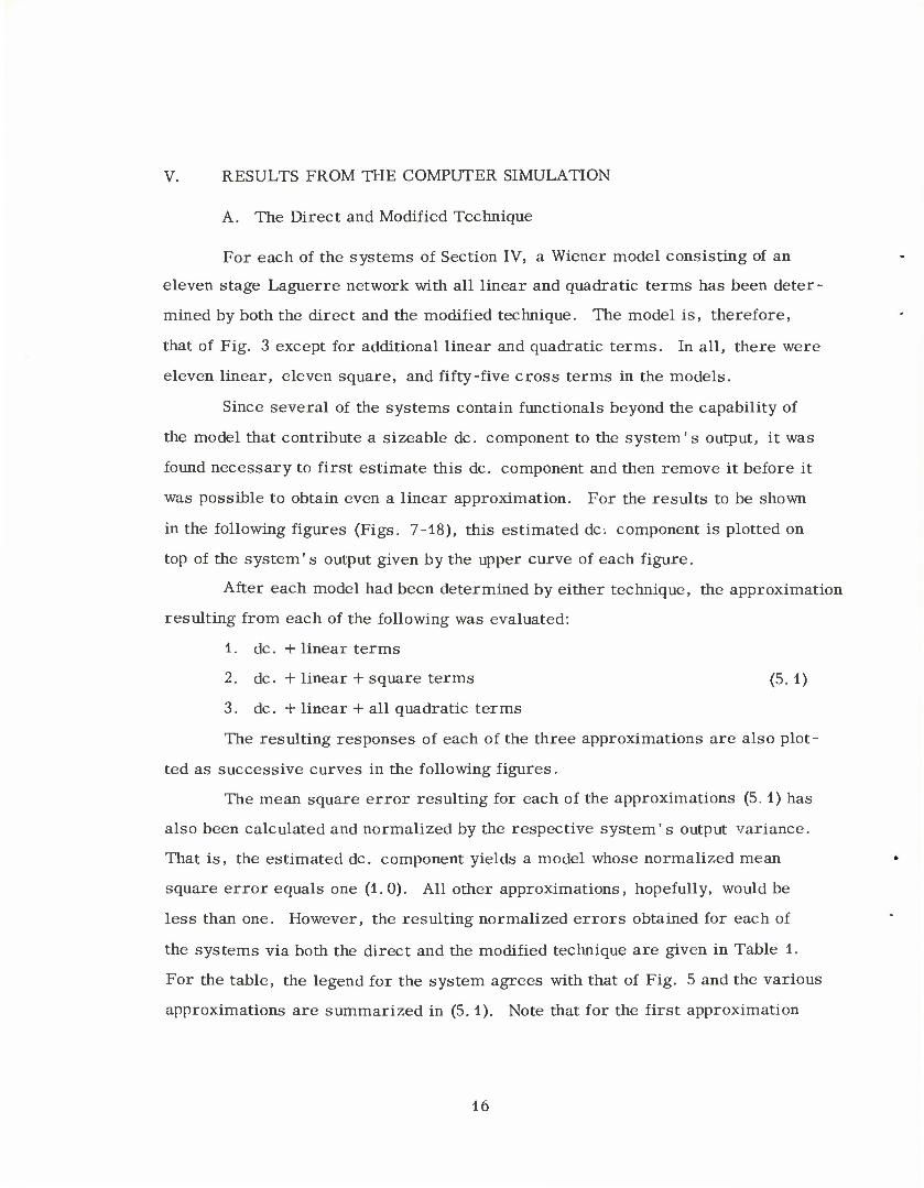
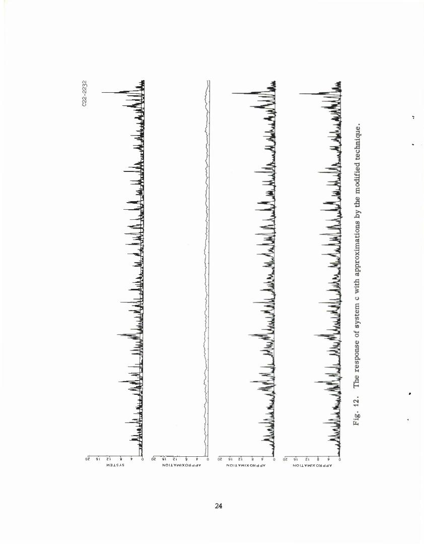
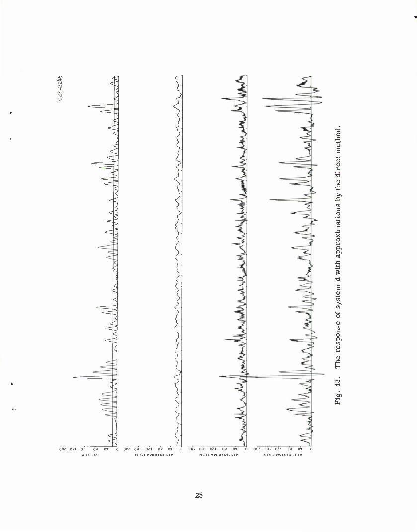
V. RESULTS FROM THE COMPUTER SIMULATION
A. The Direct and Modified Technique
For each of the systems of Section IV, a Wiener model consisting of an
eleven stage Laguerre network with all linear and quadratic terms has been deter-
mined by both the direct and the modified technique. The model is, therefore,
that of Fig. 3 except for additional linear and quadratic terms. In all, there were
eleven linear, eleven square, and fifty-five cross terms in the models.
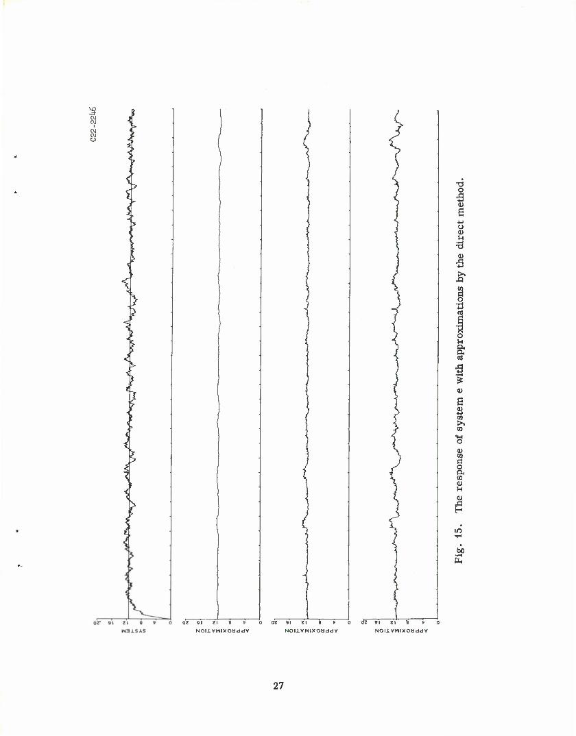
Since several of the systems contain functionals beyond the capability of
the model that contribute a sizeable dc. component to the system's output, it was
found necessary to first estimate this dc. component and then remove it before it
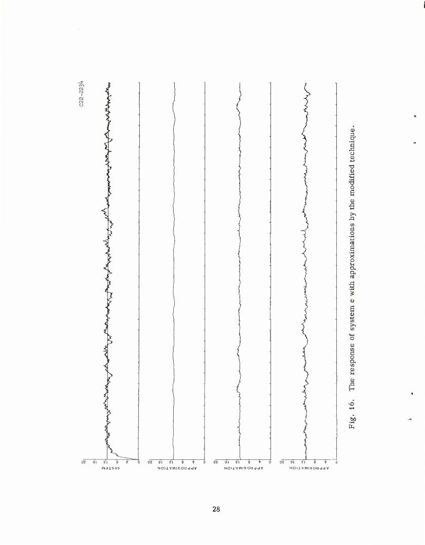
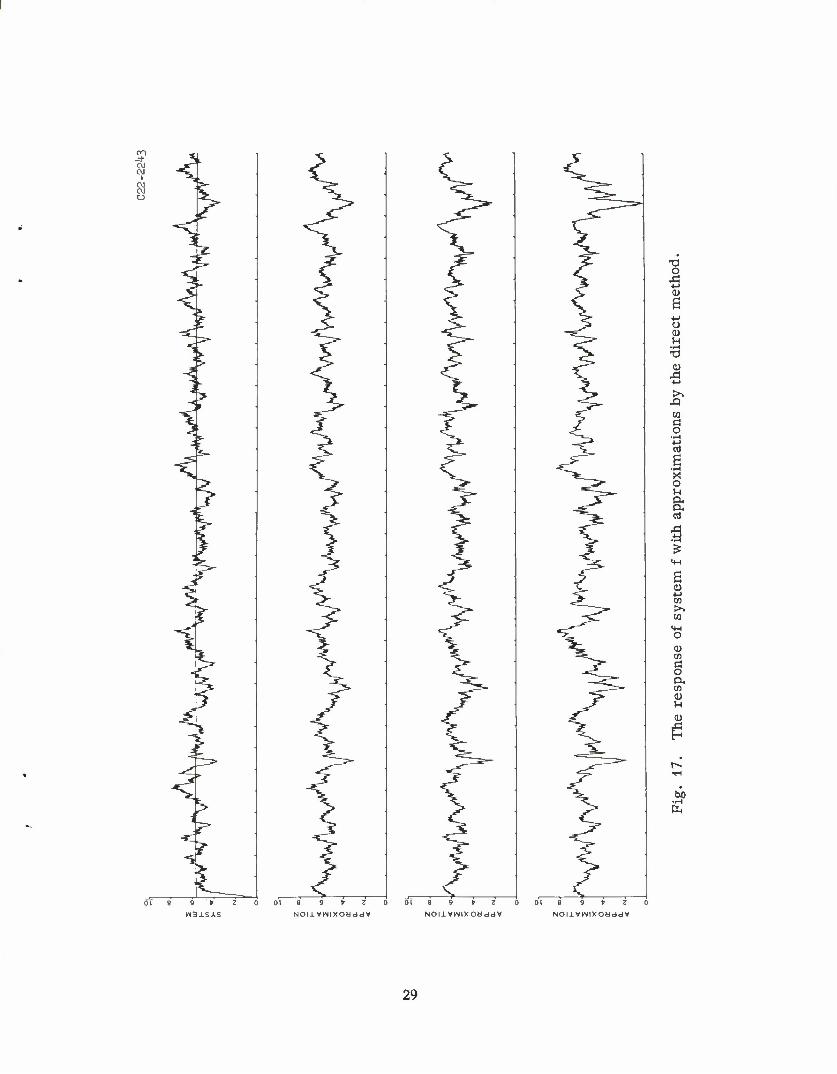
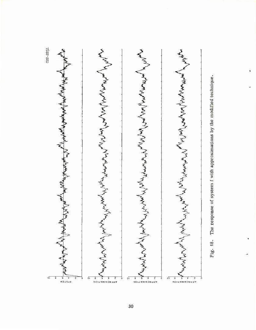
was possible to obtain even a linear approximation. For the results to be shown
in the following figures (Figs. 7-18), this estimated dc. component is plotted on
top of the system' s output given by the upper curve of each figure.
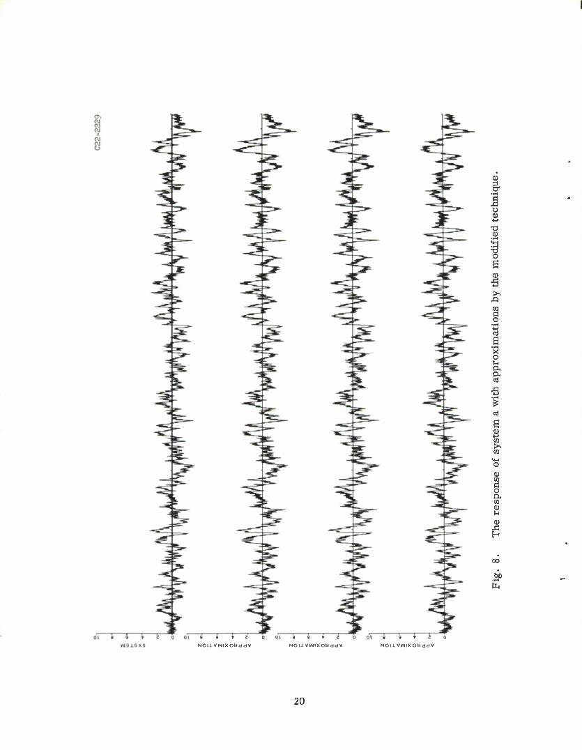
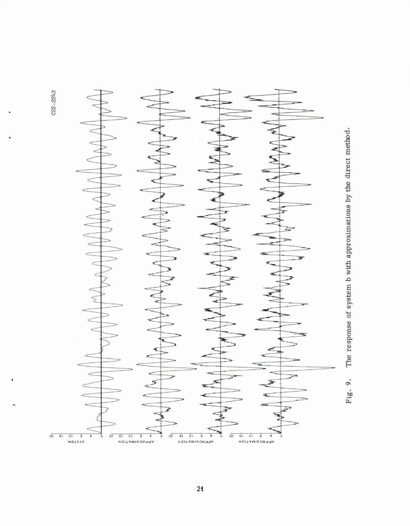
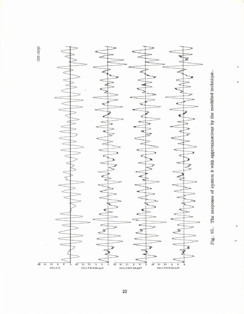
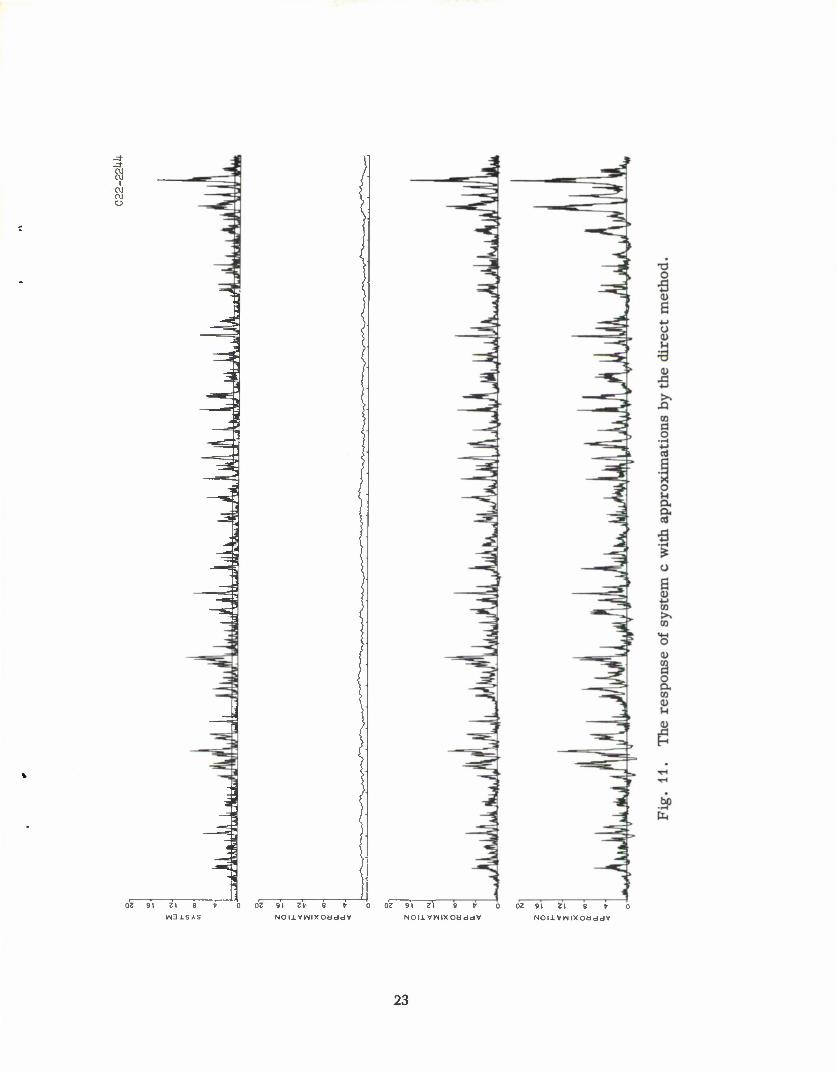
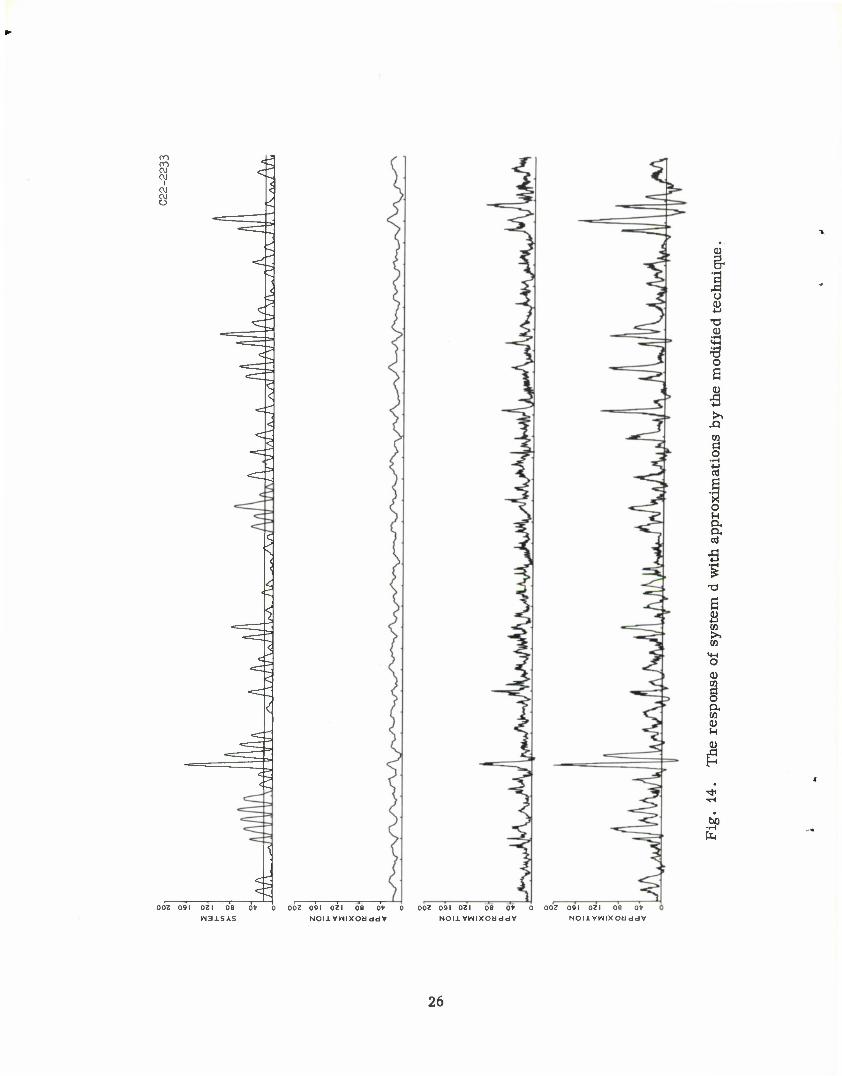
After each model had been determined by either technique, the approximation
resulting from each of the following was evaluated:
1. dc. + linear terms
2. dc. + linear + square terms (5. 1)
3. dc. + linear + all quadratic terms
The resulting responses of each of the three approximations are also plot-
ted as successive curves in the following figures.
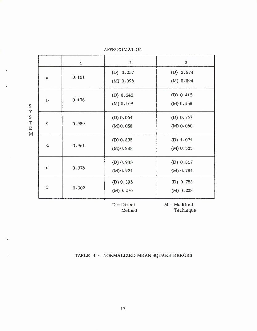
The mean square error resulting for each of the approximations (5.1) has
also been calculated and normalized by the respective system' s output variance.
That is, the estimated dc. component yields a model whose normalized mean
square error equals one (1.0). All other approximations, hopefully, would be
less than one. However, the resulting normalized errors obtained for each of
the systems via both the direct and the modified technique are given in Table 1.
For the table, the legend for the system agrees with that of Fig. 5 and the various
approximations are summarized in (5.1). Note that for the first approximation
16
APPROXIMATION
S Y S T E M
1 2 3
a 0.101 (D) 0.257
(M) 0.096
(D) 2.674
(M) 0.094
b 0.176 (D) 0.242
(M)0.169
(D) 0.415
(M) 0.158
c 0.959
(D)0.064
(M) 0.058
(D) 0.747
(M) 0.060
d 0.961 (D) 0.895
(M)0.888
(D) 1.071
(M) 0.525
e 0.976 (D) 0.935
(M)0.924
(D) 0.817
(M) 0.784
f 0.302 (D) 0.395
(M) 0.276
(D) 0.753
(M) 0.228
D = Direct Method
M = Modified Technique
TABLE 1 - NORMALIZED MEAN SQUARE ERRORS
17
(dc. + linear), both techniques yield the same model and hence only one value is
given.
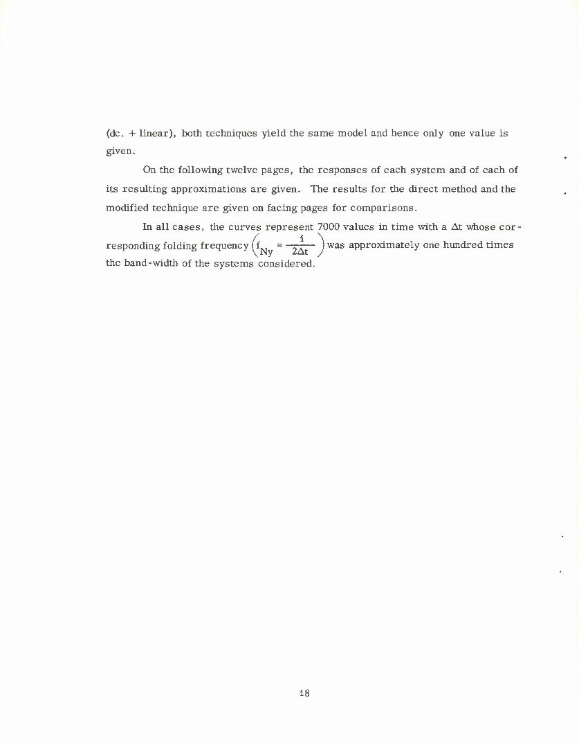
On the following twelve pages, the responses of each system and of each of
its resulting approximations are given. The results for the direct method and the
modified technique are given on facing pages for comparisons.
In all cases, the curves represent 7000 values in time with a At whose cor-
responding folding frequency (f = ) was approximately one hundred times
the band-width of the systems considered.
18
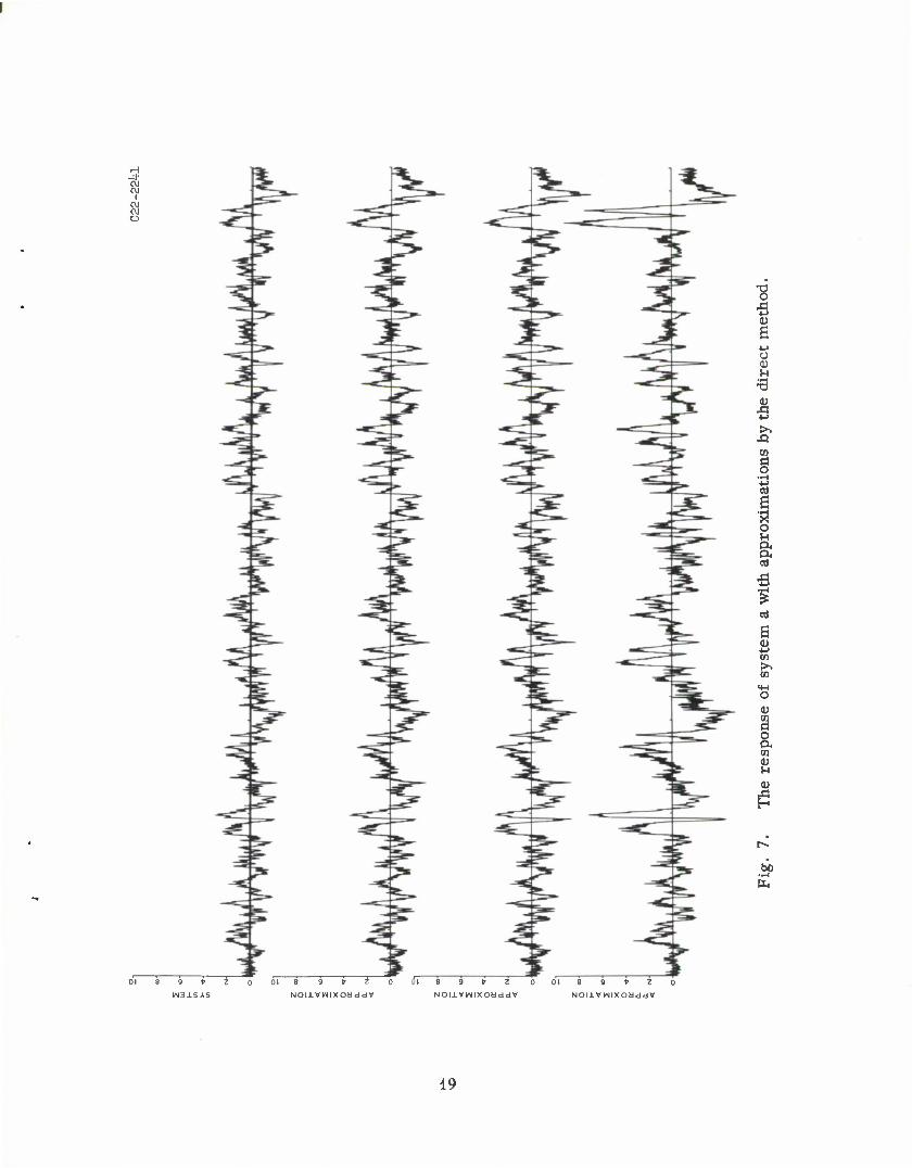
"8 I a o 0) H
•a o
B1
ctf
•a
a B to >> CO
0) CO a o ex CO
a
01 8 9 » 1 b oi 8 5 i 1 0 07 8 9 * Z 0 01 8 9 » Z 0 H31SAS NOIlVWIXOdddV NOU VHIX OM d dV NOI1VWIX Od dd V
19
o CD
•a
o B
£
I o XI
CTt | X o 6 & a
en
CO
a o a to CD H
P
00
be ft
9 t 2 NOIlVHIXOUddV
9 » Z NOUVHIXOdddV
9 t ~i~ NOIlVniXOdddV
20
cvi
8
91 Z\ 9 •
NOIlVWIXOHddV NOIlVHIXOdddV NOIlVWIXObdd*
21
i
•d .2 I o a I >>
X)
.2
O U a a
!
6 f w
o
I en
S
NOIlVniXOtlddV 91 Zl 8 V
Noiivnixoaddv NOIlVWIXOdddV
22
91 ZV 8 » NOIlVMIXOdddV
9i ~5T 9 v NOUVWIXOUddV
91 21 8 * NOIlVWIXOBHdV
23
SI
^
91 II 8 V
NOIlVWIXOdddV NOI-LVWIXOdddV 91 Z\
NOtl VWIXOdddV
24
81
002 091 03 1 08
H31SAS
0OZ 091 021 08 0»
NOIlVWIXOaddV
-a o
aj
u OJ
oj
1 o
s o M a &
! -a E OJ 4-> 00 S^ 03
a) CO
a o ex CO
OJ SH
OJ
bo
091 031 08 Ofr
NOIlVWIXOHddV
ooi 09*1 0^1 0'8 Ofr 0
NOI1 VVNIXOdddV
25
Si
003 091 03 1 09 W31SAS
003 091 031 09 0» 0 NOIlVHIXOdddV
0>
o
o B
1 X)
1 o 4-1 3
o u CL,
B 4) 00 p. 00
1 00
u
St
003 091 031 OS Of NOIlVWIXOUddV
0 003 091 031 09 of NOIlVWIXOSddV
26
3 81
B
i
OZ 91 ZI 9 »
NOIlVNIXOUddV
oz 9i zi T J-
NOIlVniXOUddV a si zi *
NOIlVWIXOUddV
o
E
l d
B
CO
CO
I CO
s cu
27
DO (M cvj
I <N t\J o
OZ 9L z\ 9 V
NOIlVHIXOdddV
91 Zl 9 •
NOIlVWIXOUddJ
02 91 ZI 9 » 0
NOIlVHIXO«dd»
28
9 fr Z
NOIlVWIXOdddV
9 fr Z
NOIlVWIXOHddV
-a O XI •l-J <L>
B o CU n
0)
•. X!
CO
§
o u ex a, ed
CO
>> CO
cu CO
d o CO
cu !-l CU
bo
f 2
NOI±VWIXOdddV
29
9 ~~f r~ NOUVWIXOMddV NOI±VHIXOdddV
"7 i~ NOIlVHIXOaddV
0) *-> GO •.
o
§ o & CO CD M
OO -rH
ti
30
B. The Gradient Technique
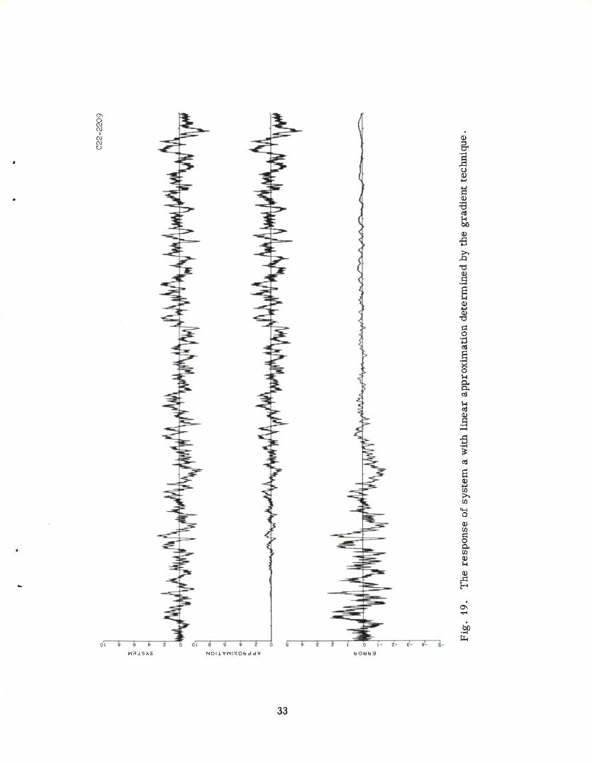
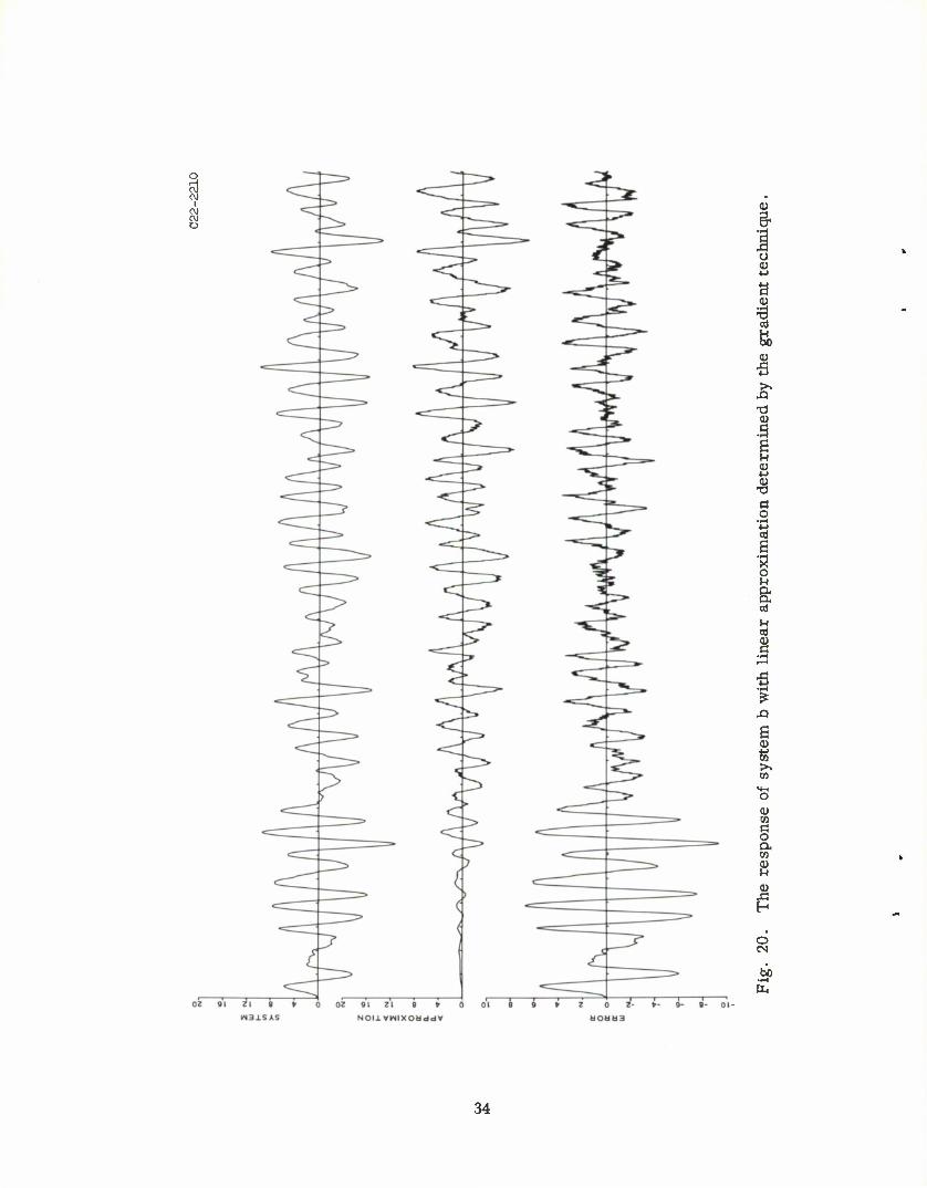
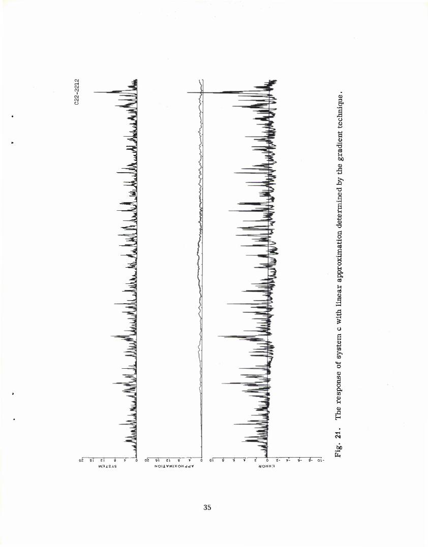
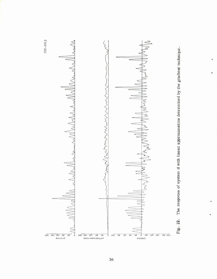
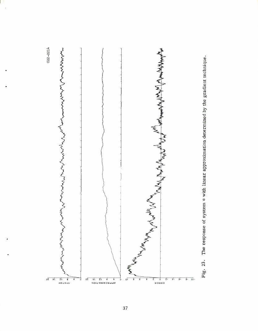
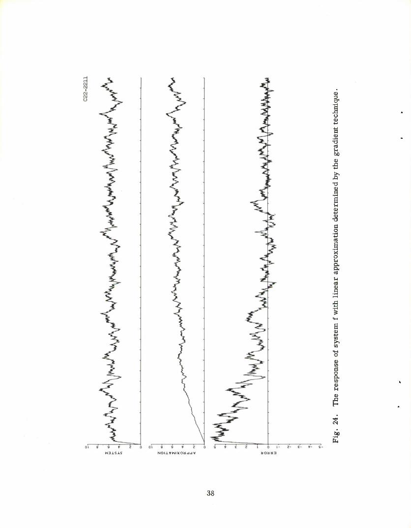
On the following pages, Figs. 19-24 give the results of an identification
program employing a gradient technique to identify only a linear model plus
bias [equivalent to approximation 1 of (5.1)] for each of the systems under con-
sideration. In all cases, the model was limited to the dc. bias plus the linear
terms on an eleven stage Laguerre network. Initially, all coefficients of the
model were set equal to zero.
In the figures following, as before, the upper curve gives the system's
response. The center curve is the response to the linear model (plus bias) and
the lower curve is the instantaneous error (between system and model) plotted to
twice the scale of the system. The convergence of the model to the system is
quite remarkable in several cases. The plotted responses represent 7000 values
(in time) in all cases.
Since the gradient technique is adaptive in nature, one cannot calculate a
residual mean square error until after the model has converged. In order to
circumvent this considerable waiting time with its greatly increased computational
requirement, and yet still provide for some comparison of this technique with
previous ones, the following calculations have been implemented.
The square of the instantaneous error was driven into a low-pass (digital)
filter whose time constant was twice that used in the averaging for the gradient
technique. The resulting filter's output gives a fair measure of the time varying
average square error. For comparison of the technique, the residual error in
the previous techniques was also driven through the same squarer/low-pass
filter combination. After 7000 values in time, this technique yielded the relative
mean square errors of Table II for the linear models to the linear systems.
31
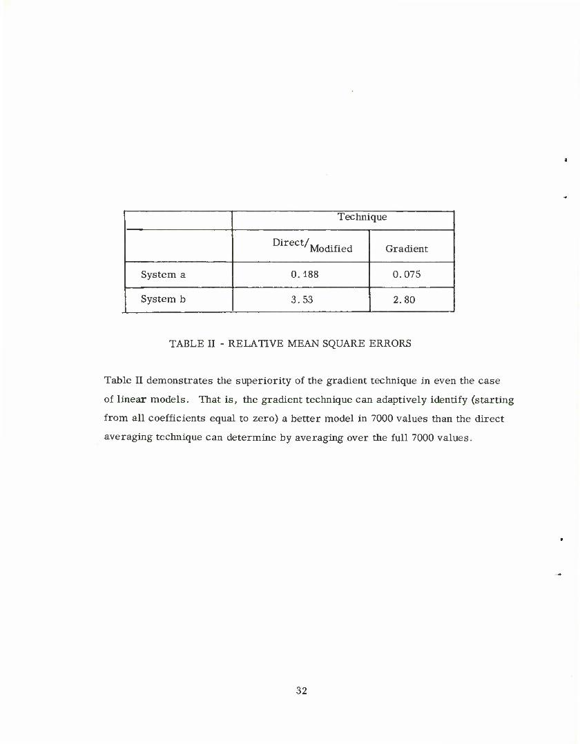
Technique
Modified Gradient
System a 0.188 0.075
System b 3.53 2.80
TABLE II - RELATIVE MEAN SQUARE ERRORS
Table II demonstrates the superiority of the gradient technique in even the case
of linear models. That is, the gradient technique can adaptively identify (starting
from all coefficients equal to zero) a better model in 7000 values than the direct
averaging technique can determine by averaging over the full 7000 values.
32
ON
1 •4->
a I a
<u
1 M
3
s
5. CO
•s cu
CO
a 0)
Nonvwixoaddv
33
81 o
0)
o CD •4->
cd
I 0)
i (3 o
3 i i o to a 3 n
1 .—I
XI
e <D
CO >> CO
CO a o ex CO u
o CN
fab
34
s <u
OZ 91 Zl 8 tr 0 OZ 91 Zl 8 * 0 01 9 9 * Z 0 Z- »- 9-
H31SAS NOIiVWIXOHddV dOMM3
u
-a I a>
a o
ex
H
•s
B CQ
>> to
•g
§ a co a> !-l u
35
<M ft]
a
002 091 021 09 Ot
kM31SAS
002 091 021 09 Ofr
NOIlVWIXOdddV
CD
o 0)
0 0)
Jn bO 0)
XI X)
1 6 M CD 4-> 0)
T3
C o
X o
R" Pi
M ed <p
6 ID
•!->
>. to
a o
u o>
P
cs CN
•9" 02 0 02- 0»-
SOHU3
36
cu CVJ
I CM OJ o
oi 9\ Fi 9 1>, I 1 ', A'
)'l 21 8 » 0 01
NOUVHIXOSddV
CO c o a w
u
en CN
37
01 9 9 fr Z
NOIlVNIXOUddV
CM
38
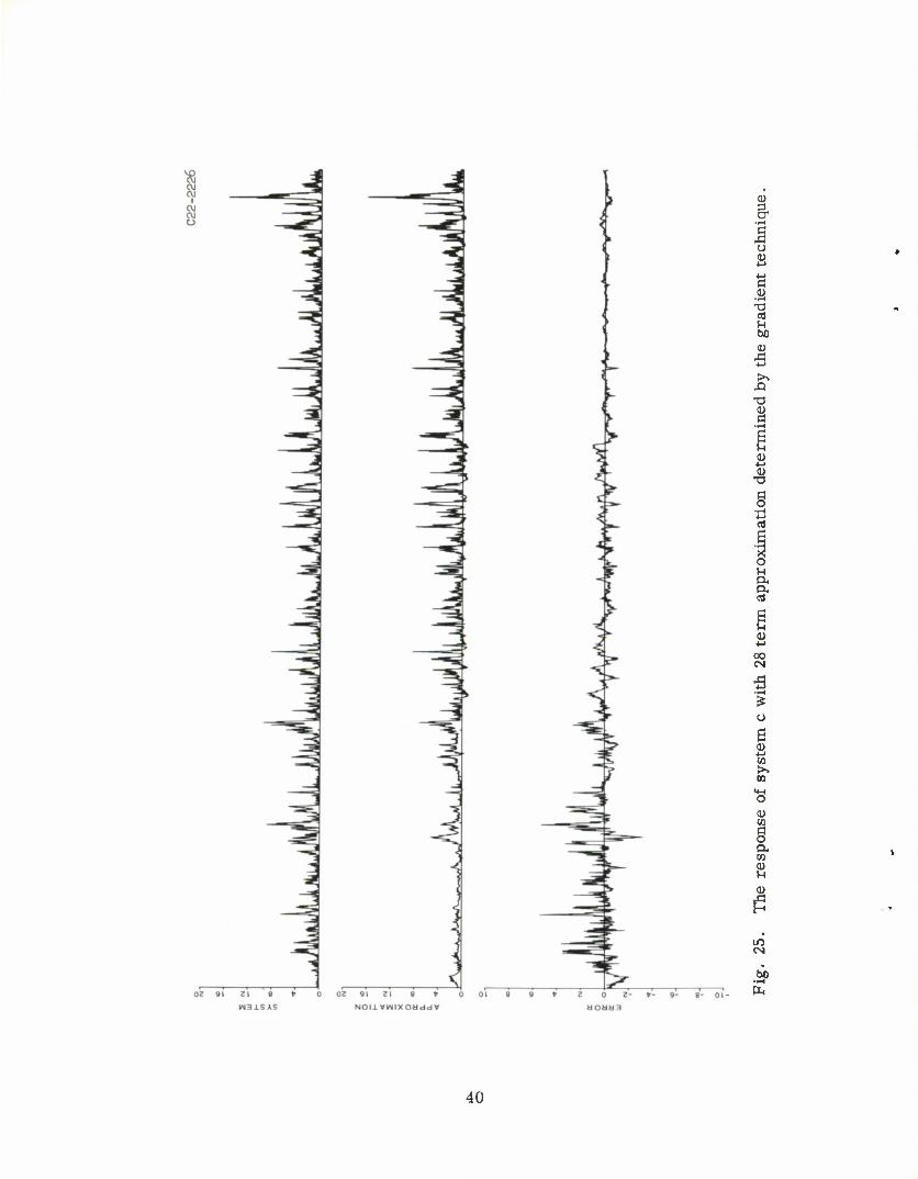
The gradient technique also has considerable merit over the direct or
modified techniques in the case of the full truncated Wiener model, i.e. , ap-
proximation 3 of (5.1). The following limitation of the gradient technique which
must be noted, however, is the following: As the number of degrees of freedom
(i.e., the number of coefficients) of the model increases, so does the time
required for convergence. Fig. 25 gives the results of the identification of
system c employing the gradient technique by a model composed of six stages
of a Laguerre network (28 terms) starting from only the dc. component. The
relative mean square errors for this model and technique and the model and
techniques of part A is:
Direct —4. 295 Modified—0.192 Gradient—0.159 (5.2)
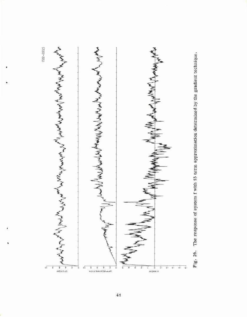
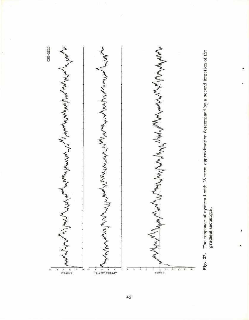
Because of the structure of the identification program, it was also a
simple matter to iterate the program using the previous iterations estimate of
the coefficients as initial values. Moreover, the subsequent iterations can in-
crease the complexity of the model. Figures 26 and 27 illustrate this technique
for the program in the case of system f (The Half-Wave Linear Detector). For
Fig. 26, the model consisted of all linear and quadratic terms (plus dc.) upon
a four stage Laguerre network. Fig. 27 is the result of a second iteration of
the program starting from the final values of Fig. 26 and with the addition of
two more stages to the network with corresponding coefficient initially equal to
zero.
39
i o
| at H bO 0)
s M
•!->
-8
o in ex a
0)
oo CM
! o
0 <D *-> W >> 05
O 0)
1 CO
u
m CN
40
LD
I B 4-1 Cfi >> CO
1) w
g a <D N
C-J
NOIlVWIXOd ddV
41
9 9 * Z
NOIlVHIXOUddV
o u (X a ed
6 R <»
•u
00 <N
"S •rH
5 <+H
6 a) *-> w >, (1) CO
& o •r-1
u .1 1 a) o •U
CO s <D (1) H € CD cd
§ &
r^ CN
bl) •i-i UH
42
VI. SUMMARY AND CONCLUSIONS
The general system identification problem has been presented as a fitting of some
mathematical model to a given physical system. The only model considered in
this report is a nonlinear model originally proposed by Norbert Wiener in 1949.
This so-called Wiener model and its truncated version, which is necessitated by
practical implementation, have been described briefly. Then three procedures for
the identification of any given system in terms of the Wiener model have been of-
fered. Finally, the report has presented results from a digital computer simulation
study (utilizing six somewhat arbitrary systems) which was designed to evaluate
the various identification procedures as well as the model itself as a basis for
system identification.
Some of the major conclusions which may be drawn from this study are the
following:
1) The implementation of a truncated Wiener model is well within the capability
of modern digital computers. For systems of modest frequency response, the cor-
responding Wiener model may well be run in real-time.
2) Of the three identification procedures considered, the gradient technique
consistently yielded a better approximation (Wiener model) for the system under
identification. This is primarily because the gradient technique does not depend
upon the orthogonality of the constituent functionals of the model and hence miti-
gates the effect of possible non-Gaussian inputs and of the finite averaging times.
Moreover, the gradient technique is also ideally suited for use in an adaptive
situation because of its ability to use existing inputs and because of the simple
recursive nature of the required algorithms.
3) For most of the systems considered for identification, the truncated
43

Wiener model has been somewhat inappropriate but then again, these arbitrary
systems were purposely chosen to be difficult in order to evaluate the Wiener
model as a basis for system identification. Other systems could have yielded
more impressive results.
44
REFERENCES
Charles R. Arnold and Kumpati S. Narendra, "The Characterization and Identification of Systems, " Craft Laboratory Technical Report No. 471 (June 18, 1965) Harvard University (AD-623 145).
2. Norbert Wiener, "Seminar in Nonlinear Networks," Research Laboratory of Electronics, Massachusetts Institute of Technology (1949) unpublished.
3. R. H. Cameron and W. T. Martin, "The Orthogonal Development of Non-linear Functions in Series of Fourier-Hermite Functionals, " Annals of Mathematics 48 (April 1947) pp. 385-392.
4. C. R. Arnold, "Laguerre Functions and the Laguerre Network - Their Properties and Digital Simulation, " Lincoln Laboratory Technical Note 1966-28 (4 May 1966) (AD-633609).
H. J. Kelley, "Method of Gradients, " Chapter 6 of Optimization Techniques, G. Leilman (ed.) Academic Press (1962).
45
UNCLASSIFIED Security Classification
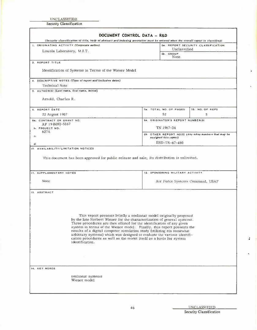
DOCUMENT CONTROL DATA - R&D (Security classification of title, body of abstract and indexing annotation must be entered when the overall report is classified)
I. ORIGINATING ACTIVITY (Corporate author)
Lincoln Laboratory, M.I.T.
2a. REPORT SECURITY CLASSIFICATION
Unclassified 2b. GROUP
None
3. REPORT TITLE
Identification of Systems in Terms of the Wiener Model
4. DESCRIPTIVE NOTES (Type of report and inclusive dates)
Technical Note 9. AUTHOR(S) (Last name, first name, initial)
Arnold, Charles R.
6. REPORT DATE
22 August 1967
7a. TOTAL NO. OF PAGES
52
7b. NO. OF REFS
5
8a. CONTRACT OR GRANT NO.
AF 19(628)-5167 b. PROJECT NO.
627A
9a. ORIGINATOR'S REPORT NUMBER(S)
TN 1967-34
9b. OTHER REPORT NO(S) (Any other numbers that may be assigned this report)
ESD-TR-67-480
10. AVAILABILITY/LIMITATION NOTICES
This document has been approved for public release and sale; its distribution is unlimited.
II. SUPPLEMENTARY NOTES
None
12. SPONSORING MILITARY ACTIVITY
Air Force Systems Command, USAF
13. ABSTRACT
This report presents briefly a nonlinear model originally proposed by the late Norbert Wiener for the characterization of general systems. Three procedures are then offered for the identification of any given system in terms of the Wiener model. Finally, this report presents the results of a digital computer simulation study (utilizing six somewhat arbitrary systems) which was designed to evaluate the various identifi- cation procedures as well as the model itself as a basis for system identification.
14. KEY WORDS
nonlinear systems Wiener model
46 UNCLASSIFIED Security Classification