Identification of parallelWiener-Hammerstein systems with a

decoupled static nonlinearity ?

M. Schoukens ∗ K. Tiels ∗ M. Ishteva ∗ J. Schoukens ∗

∗ Vrije Universiteit Brussel, Brussels, Belgium (e-mail:maarten.schoukens@vub.ac.be)

Abstract: Block-oriented models are often used to model a nonlinear system. This paperpresents an identification method for parallel Wiener-Hammerstein systems, where the obtainedmodel has a decoupled static nonlinear block. This decoupled nature makes the interpretation ofthe obtained model more easy. First a coupled parallel Wiener-Hammerstein model is estimated.Next, the static nonlinearity is decoupled using a tensor decomposition approach. Finally,the method is validated on real-world measurements using a custom built parallel Wiener-Hammerstein test system.

1. INTRODUCTION

Block-oriented models are often used to model nonlinearsystems. A block-oriented model consists of two typesof blocks: linear-time invariant (LTI) blocks and staticnonlinear (SNL) building blocks. They offer insight aboutthe system to the user due to this highly structurednature. There are many different types of block-orientedmodels, as is discussed in Giri and Bai [2010]. The simplestones are Hammerstein (SNL-LTI) and Wiener (LTI-SNL)models. These two basic block-oriented models can beextended to Wiener-Hammerstein (LTI-SNL-LTI), andHammerstein-Wiener (SNL-LTI-SNL) models by addingblocks in series. Another extension can be made to parallelHammerstein and parallel Wiener models by connecting anumber of Hammerstein or Wiener models in parallel (seeSchoukens et al. [2011] and Schoukens and Rolain [2012b]).This paper presents an identification method for parallelWiener-Hammerstein systems.

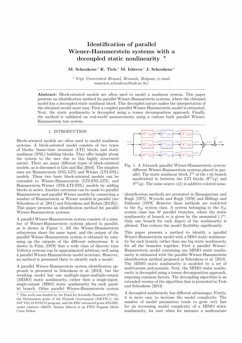
A parallel Wiener-Hammerstein system consists of a num-ber of Wiener-Hammerstein systems placed in parallel,as is shown in Figure 1. All the Wiener-Hammersteinsubsystems share the same input, and the output of theparallel Wiener-Hammerstein system is obtained by sum-ming up the outputs of the different subsystems. It isshown in Palm [1979] that a wide class of discrete timeVolterra systems can be approximated arbitrary well usinga parallel Wiener-Hammerstein model structure. However,no method is presented there to identify such a model.

A parallel Wiener-Hammerstein system identification ap-proach is presented in Schoukens et al. [2013], but theresulting model has one multiple-input-multiple-output(MIMO) static nonlinearity, rather then a single-input-single-output (SISO) static nonlinearity for each paral-lel branch. Other parallel Wiener-Hammerstein system? This work was funded by the Fund for Scientific Research (FWO),the Methusalem grant of the Flemish Government (METH-1), theIAP VII/19 DYSCO program, and the ERC advanced grant SNLSID,under contract 320378. Mariya Ishteva is an FWO Pegasus MarieCurie Fellow

Fig. 1. A 3-branch parallel Wiener-Hammerstein system:different Wiener-Hammerstein systems placed in par-allel. The static nonlinear block f [i] of the i-th branchsandwiched in between the LTI blocks H [i](q) andS[i](q). The noise source v(k) is additive colored noise.

identification methods are presented in Baumgartner andRugh [1975], Wysocki and Rugh [1976] and Billings andFakhouri [1979]. However these methods are restrictedto the SM system class. A system belonging to the SM

system class has M parallel branches, where the staticnonlinearity of branch m is given by the monomial (.)m.Only one branch for each degree of the nonlinearity isallowed. This reduces the model flexibility significantly.

This paper presents a method to identify a parallelWiener-Hammerstein model with a SISO static nonlinear-ity for each branch, rather than one big static nonlinearityfor all the branches together. First a parallel Wiener-Hammerstein model containing one MIMO static nonlin-earity is estimated with the parallel Wiener-Hammersteinidentification method proposed in Schoukens et al. [2013].The MIMO static nonlinearity is modeled by a set ofmultivariate polynomials. Next, the MIMO static nonlin-earity is decoupled using a tensor decomposition approach,imposing common factors. The decoupling algorithm is anextended version of the algorithm that is presented in Tielsand Schoukens [2013].

A decoupled nonlinearity has different advantages. Firstly,it is more easy to increase the model complexity. Thenumber of model parameters tends to grow very fastfor an increasing model complexity of a MIMO staticnonlinearity, for sure when for instance a multivariate

polynomial is used. A linear dependency of the degree isachieved when decoupled polynomials are used. Secondly,the ability to interpret the model is increased by usingdifferent SISO static nonlinearities instead of one MIMOstatic nonlinearity.

The contribution of this paper is twofold. First, this pa-per improves the decoupling method presented in Tielsand Schoukens [2013]. Second, the decoupling approachis integrated with the parallel Wiener-Hammerstein iden-tification approach that is presented in Schoukens et al.[2013], and applied on a custom built parallel Wiener-Hammerstein test system.

in Section 2, the system, signals and stochastic frameworkare introduced. Next, the proposed identification approachis explained in Section 3. Finally, the proposed method isvalidated on a measurement example in Section 4.

2. SYSTEM, SIGNALS AND STOCHASTICFRAMEWORK

This section describes the considered class of systems,introduces the noise framework and defines the signal classthat is considered in this paper.

2.1 The system class

We consider parallel Wiener-Hammerstein systems. Thesesystems consists of different Wiener-Hammerstein systemsthat share the same input signal (see Figure 1). The outputof the total system is obtained as the sum of the outputsof the different branches.

All the LTI blocks are considered to be infinite impulse re-sponse (IIR) filters, parametrized by a rational polynomialin the backward shift operator q−1:

H [i](q) =B

[i]h (q)

A[i]h (q)

=b[i]h,0 + . . .+ b

[i]h,nbh,i

q−nbh,i

a[i]h,0 + . . .+ a

[i]h,nah,i

q−nah,i

,

S[i](q) =B

[i]s (q)

A[i]s (q)

=b[i]s,0 + . . .+ b

[i]s,nbs,iq

−nbs,i

a[i]s,0 + . . .+ a

[i]s,nas,iq

−nas,i

,

where nbh,i and nah,i are the orders of the numerator anddenominator of the front dynamics of the i-th parallelbranch respectively, nbs,i and nas,i are the orders of thenumerator and denominator of the back dynamics of thei-th parallel branch.

The noiseless output y0(k) of a parallel Wiener-Hammersteinsystem is given by:

xi(k) = H [i](q)u(k), i = 1, . . . , nbr (1)

ri(k) = f [i](xi(k)), i = 1, . . . , nbr (2)

y0(k) =

nbr∑i=1

S[i](q)ri(k), (3)

where nbr is the number of parallel branches in the system,f [i](xi) is the static nonlinearity of branch i and the signalsare defined in Figure 1.

2.2 Signals and noise

The excitation signal u(k) belongs to the Riemann equiv-alence class of asymptotically normally distributed excita-tion signals as defined in Pintelon and Schoukens [2012].

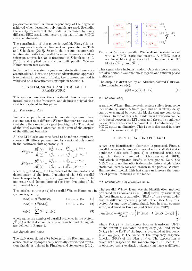
Fig. 2. A 3-branch parallel Wiener-Hammerstein modelwith a MIMO static nonlinearity. A MIMO staticnonlinear block g sandwiched in between the LTIblocks H [i](q) and S[i](q).

This signal class includes random Gaussian noise signals,but also periodic Gaussian noise signals and random phasemultisines.

The output is disturbed by an additive, colored Gaussiannoise disturbance v(k):

y(k) = y0(k) + v(k). (4)

2.3 Identifiability

A parallel Wiener-Hammerstein system suffers from someidentifiability issues. A finite gain and an arbitrary delaycan be exchanged between the blocks that are connectedin series. On top of this, a full rank linear transform can beintroduced between the LTI blocks and the static nonlinearblocks. This transforms the parallel SISO nonlinearity in aMIMO static nonlinearity. This issue is discussed in moredetail in Schoukens et al. [2013].

3. IDENTIFICATION APPROACH

A two step identification algorithm is proposed. First, aparallel Wiener-Hammerstein model with a MIMO staticnonlinear block (see Figure 2) is estimated using thealgorithm that is presented in Schoukens et al. [2013],and which is repeated briefly in this paper. Next, theMIMO static nonlinearity is decoupled into a single SISOstatic nonlinearity for each branch in the parallel Wiener-Hammerstein model. This last step can increase the num-ber of parallel branches in the model.

3.1 Identification of a coupled model

The parallel Wiener-Hammerstein identification methodpresented in Schoukens et al. [2013] starts by estimatingthe best linear approximation (BLA) of the system undertest at different operating points. The BLA Gbla of asystem for any type of input signal, best in mean squaressense, is defined in Pintelon and Schoukens [2012]:

Gbla(jωk) = arg minG(jωk)

EU

‖Y (jωk)−G(jωk)U(jωk)‖2

,

(5)

where Y (jωk) is the discrete Fourier transform (DFT)of the output y evaluated at frequency jωk, and whereU(jωk) is the DFT of the input u evaluated at frequencyjωk. Gbla(jωk) is the value of the frequency responsefunction (FRF) of the BLA at jωk. The expectation istaken with respect to the random input U . Each BLAis obtained using excitation signals that have a different

power spectrum. This changes the operating point of thesystem under test slightly for each BLA.

When input signals belonging to the Riemann equivalenceclass of asymptotically normally distributed excitation sig-nals are used, the BLA of a parallel Wiener-Hammersteinsystem is given by:

Gbla(jωk) =

nbr∑i=1

αiH[i](jωk)S[i](jωk). (6)

The scaling factors αi depend on the input power spec-trum, and on the nonlinearities that are present in thesystem. It follows from eq. (6) that the poles of the BLAare constant and independent of the applied excitationsignal, while the zeros of the BLA shift depending on theapplied excitation signal.

The BLAs of the different operating points ir areparametrized using a common denominator approach:

G[ir]bla

(q, θbla

)=d[ir]0 + d

[ir]1 q−1 + . . .+ d

[ir]nd q

−nd

c0 + c1q−1 + . . .+ cncq−nc

, (7)

where each BLA has different numerator coefficients d[ir]i ,

but they all share the same denominator coefficients ci.

Next, the dynamics present in the BLAs are decomposedover the different parallel branches of the model. To doso, the singular value decomposition (SVD) is taken of thematrix composed of the numerator coefficients:

D =

d[1]0 d

[1]1 . . . d[1]nd

d[2]0 d

[2]1 . . . d[2]nd

......

. . ....

d[R]0 d

[R]1 . . . d[R]

nd

T

, (8)

where R is the number of estimated BLAs. The SVD of Dyields an orthonormal basis for the space spanned by theD-matrix:

D = ∆blaΣblaVTbla, (9)

The matrix ∆bla contains an estimate of the numeratorcoefficients for each branch:

Gi(q) =δ[i]0 + δ

[i]1 q

−1 + . . .+ δ[i]ndq

−nd

c0 + c1q−1 + . . .+ cncq−nc

, (10)

where δ[i]j is the element of the j-th row and i-th column

of the matrix ∆bla. An estimate of the number of parallelbranches nbr present in the system is obtained by lookingat the spectrum of the singular values of D. Gi(q) is anestimate of the dynamics that are present in branch i ofthe parallel Wiener-Hammerstein model.

Finally, the estimated dynamics of each branch of theparallel Wiener-Hammerstein model need to be allocatedto the front and back LTI blocks of the model. To do so, allcombinations of poles and zeros in the different blocks arescanned, and a MIMO static nonlinear block is estimatedfor each combination with a multivariate polynomial whichis linear in the parameters. Finally, the model with thesmallest simulation error is selected. The parameters of theselected model are optimized further using a Levenberg-Marquardt nonlinear optimization algorithm to refine themodel estimate. A more detailed description of this stepin the algorithm can be found in Schoukens et al. [2013].

In this paper, a low order multivariate polynomial isused to model the MIMO static nonlinearity to limit thenumber of coefficients. The next section presents a methodto decouple the MIMO static nonlinearity to one SISOstatic nonlinearity for each branch. The complexity of themodels that describe the decoupled static nonlinearities isincreased in a later step. This decreases the model error,while keeping the number of parameters in the modelrelatively low (compared to a high order MIMO staticnonlinearity).

3.2 Decoupling the static nonlinearity

The decoupling method generates starting values for theparameters of the decoupled Wiener-Hammerstein model,described by:

xi(k) = H [i](q)u(k), i = 1, . . . , nr (11)

ri(k) = f [i](xi(k)), i = 1, . . . , nr (12)

y(k) =

nr∑i=1

S[i](q)ri(k), (13)

starting from its coupled polynomial representation:

xi(k) = H [i](q)u(k), i = 1, . . . , nbr (14)

ri(k) = g[i](x(k)), i = 1, . . . , nbr (15)

y(k) =

nbr∑i=1

S[i](q)ri(k), (16)

where x(k) = [x1(k), · · · , xnbr(k)]T . As already pointed

out, the decoupling step can increase the number ofbranches (nr can be larger than nbr), but the goal is tokeep the number of branches nr small.

Some methods already exist to decouple the polynomialrepresentations in Volterra models (see Favier and Bouilloc[2009]), and parallel Wiener models (see Schoukens andRolain [2012a]). For example, the method in Schoukensand Rolain [2012a] splits the polynomial in a sum ofhomogeneous polynomials, and uses tensor decompositionmethods to eliminate the cross-terms in each homogeneouspolynomial separately. This technique can be directly ap-plied to each polynomial g[i](x(k)), and is in Tiels andSchoukens [2013] referred to as “separate decoupling”.This results in a sum of optimally decoupled polynomialrepresentations (optimal in the sense of the smallest num-ber of branches), but the total number of branches is notnecessarily optimal. Two other methods are presented inTiels and Schoukens [2013], referred to as “simultaneoushomogeneous” and “simultaneous all”, that can result ina smaller total number of branches. This is realized byimposing common factors in the tensor decompositions.The main idea behind these methods is to impose that theresulting SISO polynomials share the same input signals,thus keeping the number of input filters H [i](q) small. The“simultaneous all” approach suffers from the drawbackthat, although the same input dynamics are shared forall polynomials, the output dynamics in general differfor different degrees of nonlinearity. Another drawback ofthe method is that the coefficients of the resulting SISOpolynomials are all equal to one.

Here we present an improved version of the “simultaneousall” method. Without loss of generality, the focus is

on quadratic and cubic polynomials. Compared to the“simultaneous all” approach in Tiels and Schoukens [2013],in this paper, branches that share the same input dynamicsare imposed to share the same output dynamics as well.Moreover, the flexibility of each branch in the decoupledstructure is increased by allowing arbitrary coefficientsβ for the SISO polynomials. Although this increases thecomplexity of the optimization problem, the increasedflexibility of each branch allows for a smaller total numberof branches.

Assume that g[i](x(k)) is the sum of a quadratic and acubic homogeneous polynomial:

g[i](x(k)) =

nbr∑j1,j2=1

γ[i]j1j2

xj1(k)xj2(k)

+

nbr∑j1,j2,j3=1

w[i]j1j2j3

xj1(k)xj2(k)xj3(k),

(17)

with Γ[i] the symmetric matrix of polynomial coefficients

γ[i]j1j2

, and W [i] the symmetric tensor of polynomial coef-

ficients w[i]j1j2j3

. The main tool to decouple these matricesand tensors will be the canonical polyadic decomposition(CPD) (see Carroll and Chang [1970], Harshman [1970],Kolda and Bader [2009]). The CPD approximates a tensor- in least squares sense - by a sum of rank-one tensors. Say,

for example, that W [i] has a CPD

W [i] ≈nr∑r=1

ψ[i]r pr pr pr, (18)

where denotes the tensor product. This means thatelement-wise:

w[i]j1j2j3

≈nr∑r=1

ψ[i]r p

[i]j1rp[i]j2rp[i]j3r. (19)

The cubic multivariate homogeneous polynomial described

by W [i] is thus transformed into a sum of nr univariate

homogeneous polynomials ψ[i]r x3r(k), with xr = pTr x(k).

The CPD is often calculated via an alternating least-squares (ALS) approach (see e.g. Kolda and Bader [2009]).Recently, other algorithms to calculate the CPD of a tensorwere proposed in Sorber et al. [2013a] that obtain a betteroverall performance than ALS.

To impose that the univariate polynomials, obtained

from decoupling all the matrices Γ[i] and all the tensors

W [i], share the same input signals xr, these matricesand tensors are stacked in a partially symmetric tensorT ∈ R(nbr+1)×(nbr+1)×(nbr+1)×2×nbr , such that:

T ≈nr∑r=1

[pr1

][pr1

][pr1

][β2rβ3r

]mr, (20)

where,mjr = φ[j]r , j = 1, . . . , nbr. (21)

The one stacked with the pr vector imposes a partialsymmetry in the matrix, which is used during the decom-position step. The entries of T are given by 1 2 :1 Due to symmetry tj1j2(nbr+1)jj4 is also equal to tj1(nbr+1)j2jj4and t(nbr+1)j1j2jj4 for j = 1, 2.2 Note that the entries given by (24) and (25) are unknown, however,this issue can be handled by treating them as missing elements inthe tensor to be decomposed.

tj1j2j32j4 = w[j4]j1j2j3

, (22)

tj1j2(nbr+1)1j4 = γ[j4]j1j2

, (23)

tj1j2j31j4 ≈nr∑r=1

pj1rpj2rpj3rβ2rφ[j4]r , (24)

tj1j2(nbr+1)2j4 ≈nr∑r=1

pj1rpj2rβ3rφ[j4]r , (25)

for j1, j2, j3, j4 = 1, . . . , nbr.

The tensor T is decoupled using the Tensorlab toolboxby Sorber et al. [2013b] which can handle missing entriesand partial symmetry. This results in a decoupled parallelWiener-Hammerstein model, as described by (13). Theinput dynamics, SISO polynomials, and output dynamicsof the decoupled model are given by:

H [r](q) =

nbr∑j=1

pjrH[j](q), (26)

f [r](xr(k)) = β2rx2r(k) + β3rx

3r(k), (27)

S[r](q) =

nbr∑j=1

φ[j]r S[j](q), (28)

for r = 1, . . . , nr. The resulting model has nr branches,where nr is set by the user.

Note that the optimization does not take into account theactual input/output data. The optimization is only donestarting from the estimated polynomial coefficients. Thisallows us to generate relatively quickly decent startingvalues for the parameters of the decoupled structure. Ina next step, these parameters can be further optimizedstarting from the input/output data.

4. MEASUREMENT EXAMPLE

The proposed method is illustrated on an experimentalsetup.

4.1 System and measurement setup

The device under test (DUT) is a 2-branch parallelWiener-Hammerstein system. The front and back LTIblocks of each branch are third order IIR filters. The staticnonlinearity of each branch is realized with a diode-resistornetwork.

The signals are generated by an arbitrary waveform gen-erator (AWG), the Agilent/HP E1445A, at a samplingfrequency of 625 kHz. An internal low-pass filter with acut-off frequency of 250 kHz is used as a reconstructionfilter for the input signal. The in- and output signals ofthe system are measured by the alias protected acquisitionchannels (Agilent/HP E1430A) at a sampling frequency of78 kHz. The AWG and acquisition cards are synchronizedto avoid leakage errors.

Finally, buffers with a high input impedance, added be-tween the acquisition cards and the in- and output of theDUT, avoid that the circuit is loaded by the 50 Ohm inputimpedance of the acquisition card. The buffers are verylinear (≈ 85 dBc at full scale and 1 MHz) up to 10 V peakto peak, and have an input impedance of 1 MΩ and a 50Ω output impedance.

4.2 Signal generation

The input signal u(k) is a random phase multisine (seePintelon and Schoukens [2012]) containing N = 131072samples with a flat amplitude spectrum. The excitedfrequency band ranges from fs

N to fs2 , viz.:

u(k) = A

N/2∑n=1

cos(2πnfsNk + φn), (29)

The phases φn are independent uniformly distributed ran-dom variables ranging from 0 to 2π. Twenty realizationsof the multisines are used. The input signal is applied at 5different rms values that are linearly distributed between100 mV and 1 V.

The signals are measured at a sampling frequency of 78kHz, which is 8 times slower than the sampling frequencyat the generator side, resulting in N = 16384 samples perperiod.

4.3 Model estimation

First, the BLAs of the DUT are estimated at the differentoperating points (or input amplitudes in this case). TheBLAs are parameterized using a discrete time LTI modelof order 12 in both the numerator and denominator.

Starting from these BLAs, an initial 2-branch coupledparallel Wiener-Hammerstein model is estimated. Themodel has 2 parallel branches, and the MIMO staticnonlinearity is modeled with a 3rd order multivariatepolynomial. A static nonlinearity of low degree is used suchthat the number of parameters in the model description islimited. However, this simple static nonlinearity is ableto provide sufficiently good initial values for the followingsteps.

Next, the low order multivariate polynomial is decoupledusing the approach that is presented in Section 3.2, and adecoupled parallel 2-branch Wiener-Hammerstein modelwith 3rd order polynomial SISO static nonlinearities isconstructed based on this result.

Finally, the static nonlinearities in the low order decoupledparallel Wiener-Hammerstein model are replaced by poly-nomials of order 15. A Levenberg-Marquardt optimizationalgorithm is applied on the high order decoupled 2-branchparallel Wiener-Hammerstein model to further optimizethe parameters. In this step, other static nonlinear modelssuch as artificial neural networks can also be used to modelthe static nonlinearities of the model.

4.4 Model validation

The model is validated using a different realization of therandom phase multisines that are described in Section4.2. The results of the validation are shown in Table 1and Figure 3. Table 1 shows three figures of merit: therms value of the simulation error rms(e), the standarddeviation of the simulation error σe, and the mean valueof the simulation error µe, as defined below:

rms(e) =

√√√√ 1

N

N∑k=1

e2(k), (30)

σe =

√√√√ 1

N

N∑k=1

(e(k)− µe)2, (31)

µe =1

N

N∑k=1

e(k), (32)

where e(k) is the difference between the measured outputy(k) and the modeled output y(k).

The low order decoupled model has a clear performanceloss compared to the coupled model. However, it provides agood starting value to further increase the static nonlinear-ity model complexity for further optimization. Increasingthe model order in the coupled model is very costly inthe number of parameters. Describing the coupled staticnonlinearity with a 15th order multivariate polynomialwould require 136 parameters, where only 32 parametersare needed to describe the 15th order polynomials of thedecoupled static nonlinear blocks.

The high order decoupled model performs very well. Figure3 shows that the model error is about 50 dB lower thanthe output spectrum for an excitation signal with an rmsvalue of 550 mV. Furthermore, the model error is about30 dB lower than the total distortion level of the outputspectrum. The total distortion level includes the noisedistortions and distortions due to the nonlinear behaviorof the system (see Pintelon and Schoukens [2012]). Thisshows that the model describes the nonlinear behavior ofthe system very well. Finally, the model error is 10 to 20 dBhigher than the noise floor. This suggests that the modelquality can still be improved, for instance by increasingthe order of the static nonlinearity even more.

The static nonlinearities that are present in the high orderdecoupled model are shown in Figure 4. They show asaturating behavior. This is what is to be expected sincethe static nonlinearities in the system are generated byelectrical diode-resistor networks.

5. CONCLUSION

This paper presents an improved method to decouplea MIMO static nonlinearity described by multivariatepolynomials into different SISO polynomial static non-linearities using tensor decomposition methods. This de-coupling approach is integrated with a parallel Wiener-Hammerstein identification method to obtain parallelWiener-Hammerstein models with different SISO staticnonlinearities rather than one MIMO static nonlinearity.The approach is applied on a measurement example toshow the good performance of the proposed method.

REFERENCES

S.L. Baumgartner and W.J. Rugh. Complete identifica-tion of a class of nonlinear systems from steady statefrequency response. IEEE Trans. Circuits Syst., 22(9):753–759, 1975.

S.A. Billings and S.Y. Fakhouri. Identification of non-linear Sm systems. International Journal of SystemsScience, 10(10):1401–1408, 1979.

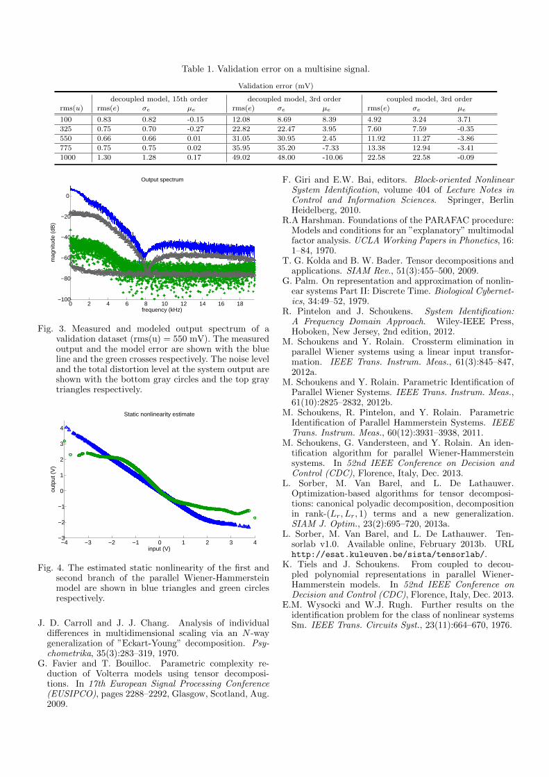
Table 1. Validation error on a multisine signal.

Validation error (mV)

decoupled model, 15th order decoupled model, 3rd order coupled model, 3rd orderrms(u) rms(e) σe µe rms(e) σe µe rms(e) σe µe

100 0.83 0.82 -0.15 12.08 8.69 8.39 4.92 3.24 3.71

325 0.75 0.70 -0.27 22.82 22.47 3.95 7.60 7.59 -0.35

550 0.66 0.66 0.01 31.05 30.95 2.45 11.92 11.27 -3.86

775 0.75 0.75 0.02 35.95 35.20 -7.33 13.38 12.94 -3.41

1000 1.30 1.28 0.17 49.02 48.00 -10.06 22.58 22.58 -0.09

0 2 4 6 8 10 12 14 16 18−100

−80

−60

−40

−20

0

Output spectrum

frequency (kHz)

mag

nitu

de (

dB)

Fig. 3. Measured and modeled output spectrum of avalidation dataset (rms(u) = 550 mV). The measuredoutput and the model error are shown with the blueline and the green crosses respectively. The noise leveland the total distortion level at the system output areshown with the bottom gray circles and the top graytriangles respectively.

−4 −3 −2 −1 0 1 2 3 4−3

−2

−1

0

1

2

3

4

input (V)

outp

ut (

V)

Static nonlinearity estimate

Fig. 4. The estimated static nonlinearity of the first andsecond branch of the parallel Wiener-Hammersteinmodel are shown in blue triangles and green circlesrespectively.

J. D. Carroll and J. J. Chang. Analysis of individualdifferences in multidimensional scaling via an N -waygeneralization of ”Eckart-Young” decomposition. Psy-chometrika, 35(3):283–319, 1970.

G. Favier and T. Bouilloc. Parametric complexity re-duction of Volterra models using tensor decomposi-tions. In 17th European Signal Processing Conference(EUSIPCO), pages 2288–2292, Glasgow, Scotland, Aug.2009.

F. Giri and E.W. Bai, editors. Block-oriented NonlinearSystem Identification, volume 404 of Lecture Notes inControl and Information Sciences. Springer, BerlinHeidelberg, 2010.

R.A Harshman. Foundations of the PARAFAC procedure:Models and conditions for an ”explanatory” multimodalfactor analysis. UCLA Working Papers in Phonetics, 16:1–84, 1970.

T. G. Kolda and B. W. Bader. Tensor decompositions andapplications. SIAM Rev., 51(3):455–500, 2009.

G. Palm. On representation and approximation of nonlin-ear systems Part II: Discrete Time. Biological Cybernet-ics, 34:49–52, 1979.

R. Pintelon and J. Schoukens. System Identification:A Frequency Domain Approach. Wiley-IEEE Press,Hoboken, New Jersey, 2nd edition, 2012.

M. Schoukens and Y. Rolain. Crossterm elimination inparallel Wiener systems using a linear input transfor-mation. IEEE Trans. Instrum. Meas., 61(3):845–847,2012a.

M. Schoukens and Y. Rolain. Parametric Identification ofParallel Wiener Systems. IEEE Trans. Instrum. Meas.,61(10):2825–2832, 2012b.

M. Schoukens, R. Pintelon, and Y. Rolain. ParametricIdentification of Parallel Hammerstein Systems. IEEETrans. Instrum. Meas., 60(12):3931–3938, 2011.

M. Schoukens, G. Vandersteen, and Y. Rolain. An iden-tification algorithm for parallel Wiener-Hammersteinsystems. In 52nd IEEE Conference on Decision andControl (CDC), Florence, Italy, Dec. 2013.

L. Sorber, M. Van Barel, and L. De Lathauwer.Optimization-based algorithms for tensor decomposi-tions: canonical polyadic decomposition, decompositionin rank-(Lr, Lr, 1) terms and a new generalization.SIAM J. Optim., 23(2):695–720, 2013a.

L. Sorber, M. Van Barel, and L. De Lathauwer. Ten-sorlab v1.0. Available online, February 2013b. URLhttp://esat.kuleuven.be/sista/tensorlab/.

K. Tiels and J. Schoukens. From coupled to decou-pled polynomial representations in parallel Wiener-Hammerstein models. In 52nd IEEE Conference onDecision and Control (CDC), Florence, Italy, Dec. 2013.

E.M. Wysocki and W.J. Rugh. Further results on theidentification problem for the class of nonlinear systemsSm. IEEE Trans. Circuits Syst., 23(11):664–670, 1976.