This article was downloaded by: [New York University]On: 03 June 2015, At: 14:00Publisher: Taylor & FrancisInforma Ltd Registered in England and Wales Registered Number: 1072954 Registered office: Mortimer House,37-41 Mortimer Street, London W1T 3JH, UK

Click for updates

International Journal of Systems SciencePublication details, including instructions for authors and subscription information:http://www.tandfonline.com/loi/tsys20

Adaptive control of Hammerstein–Wiener nonlinearsystemsBi Zhanga, Hyokchan Honga & Zhizhong Maoab

a Institute of Automation, College of Information Science & Engineering, NortheasternUniversity, Shenyang P.R. Chinab State Key Laboratory of Synthetical Automation for Process Industries, NortheasternUniversity, Shenyang P.R. ChinaPublished online: 21 Oct 2014.

To cite this article: Bi Zhang, Hyokchan Hong & Zhizhong Mao (2014): Adaptive control of Hammerstein–Wiener nonlinearsystems, International Journal of Systems Science, DOI: 10.1080/00207721.2014.971089

To link to this article: http://dx.doi.org/10.1080/00207721.2014.971089

PLEASE SCROLL DOWN FOR ARTICLE

Taylor & Francis makes every effort to ensure the accuracy of all the information (the “Content”) containedin the publications on our platform. However, Taylor & Francis, our agents, and our licensors make norepresentations or warranties whatsoever as to the accuracy, completeness, or suitability for any purpose of theContent. Any opinions and views expressed in this publication are the opinions and views of the authors, andare not the views of or endorsed by Taylor & Francis. The accuracy of the Content should not be relied upon andshould be independently verified with primary sources of information. Taylor and Francis shall not be liable forany losses, actions, claims, proceedings, demands, costs, expenses, damages, and other liabilities whatsoeveror howsoever caused arising directly or indirectly in connection with, in relation to or arising out of the use ofthe Content.

This article may be used for research, teaching, and private study purposes. Any substantial or systematicreproduction, redistribution, reselling, loan, sub-licensing, systematic supply, or distribution in anyform to anyone is expressly forbidden. Terms & Conditions of access and use can be found at http://www.tandfonline.com/page/terms-and-conditions

International Journal of Systems Science, 2014http://dx.doi.org/10.1080/00207721.2014.971089

Adaptive control of Hammerstein–Wiener nonlinear systems

Bi Zhanga, Hyokchan Honga and Zhizhong Maoa,b,∗

aInstitute of Automation, College of Information Science & Engineering, Northeastern University, Shenyang P.R. China; bState KeyLaboratory of Synthetical Automation for Process Industries, Northeastern University, Shenyang P.R. China

(Received 23 December 2013; accepted 26 September 2014)

The Hammerstein–Wiener model is a block-oriented model, having a linear dynamic block sandwiched by two static nonlinearblocks. This note develops an adaptive controller for a special form of Hammerstein–Wiener nonlinear systems which areparameterized by the key-term separation principle. The adaptive control law and recursive parameter estimation are updatedby the use of internal variable estimations. By modeling the errors due to the estimation of internal variables, we establishconvergence and stability properties. Theoretical results show that parameter estimation convergence and closed-loop systemstability can be guaranteed under sufficient condition. From a qualitative analysis of the sufficient condition, we introducean adaptive weighted factor to improve the performance of the adaptive controller. Numerical examples are given to confirmthe results in this paper.

Keywords: Hammerstein–Wiener nonlinear system; adaptive control; convergence properties; closed-loop system stability;adaptive weighted factor

1. Introduction

There exist many methods for parameter estimation andadaptive control for linear dynamic systems (Chen & Guo,1991; Goodwin & Sin, 1984; Ljung, 1999). In practice,however, almost all the physical systems are nonlinear tosome extent. As is reported recently in many papers, theso-called block-oriented models have turned out to be veryuseful in modeling and controlling nonlinear systems (Giri& Bai, 2010). Typically, such models are Hammersteinmodel (H, linear time-invariant (LTI) block following somestatic nonlinear block), Wiener model (W, LTI block pre-ceding some static nonlinear block), Hammerstein–Wienermodel (H–W, LTI block sandwiched by two static nonlin-ear blocks), and Wiener–Hammerstein model (W–H, a staticnonlinear blocks sandwiched by two LTI blocks).

Many approaches have been proposed to identify block-oriented nonlinear models. We list only some of the con-structive contributions to readers. Roughly speaking, themost commonly used approaches are the iterative method(Giri, Rochdi, & Chaoui, 2009; Liu & Bai, 2007; Zhu,2002), the blind identification method (Bai, 2002), the over-parameterized method (Bai, 1998; Ding & Chen, 2005),and the key-term separation identification method (Voros,1999,2003; Yu, Mao, & Jia, 2013). Identification of block-oriented models is one of the key challenges explored bymany researchers. Up to now, the identification methods areattractive, advanced, and successful.

∗Corresponding author. Email: maozhizhong@ise.neu.edu.cn

In contrast to the contributions for block-oriented non-linear systems identification, much less efforts have beendone to design controllers for block-oriented models, whichis another key challenge omitted by many researchers. In theprevious work, Dolanc and Strmcnik (2008) and Lv and Ren(2012) have proposed nonlinear controllers based on theclassic linear pole placement principle. The model parame-ters are obtained by the ‘off-line’ identification, conductedprior to the control experiment. In Fruzzetti, Palazoglu, andMcDonald (1997), Harinischmacher and Marquardt (2007),and Patikirikorala, Wang, Colman, and Han (2012), non-linear model predictive controllers are with applications torealistic process conditions. Assuming the state is measur-able, Bloemen, Boom, and Verbruggen (2001) and Bloemenet al. (2001) have proposed robust model predictive con-trollers. Bloemen’s work has been further studied in Dingand Huang (2007) and Ding and Ping (2012) in the sensethat the state is unmeasurable. In Kim, Rios-Patron, andBraatz (2012), a robust nonlinear internal model controlleris reported.

In view of the uncertainties in the block-oriented mod-els, an adaptive controller can achieve global stability andsatisfactory output tracking performance simultaneously(Moreno-Valenzuela, 2013). In Chen (2007), Ding, Chen,and Iwai (2007), Figueroa, Cousseau, Werner, and Laakso(2007), Kung and Womack (1983), Pajunen (1992), andZhao and Chen (2009), adaptive controllers are studied

C© 2014 Taylor & Francis

Dow

nloa

ded

by [

New

Yor

k U

nive

rsity

] at

14:

00 0

3 Ju

ne 2

015

2 B. Zhang et al.

for H and W models, which are consisted of two blocksand contain only one nonlinear part. As far as the authors’known, there are few adaptive controllers designed for H–W systems, which is the motivation of this work. As well,this is the first contribution of this work.

In this work, in order to derive an adaptive controllerfor H–W systems, the first issue is to establish a param-eterized H–W model, which is suitable for identificationusing the available data. Recall the most commonly usedidentification methods introduced in the second paragraph.Some special persistent excitation input signals are re-quired in the iterative method and the blind identifica-tion method. Therefore, the methods above cannot be usedto serve as a recursive estimator in adaptive controllerdesign.

Up to now, the over-parameterized method has beenused successfully as recursive estimator in adaptive con-trol for H and W systems (Chen, 2007; Ding et al., 2007;Figueroa et al., 2007; Kung & Womack, 1983; Pajunen,1992; Zhao & Chen, 2009). In these contributions, block-oriented models (only H and W systems considered) are pa-rameterized to be bilinear models. Then, convergence andstability analysis can be viewed as an extension of the linearcase well studied in Chen and Guo (1991), Goodwin andSin (1984), and Ljung (1999). However, if H–W systems areaddressed, it is difficult and unlikely to obtain bilinear para-metric models, which means that the over-parameterizedmethod seems not to work.

For adaptive control of H–W systems, an attractive pa-rameterization method is by the key-term separation princi-ple, which has seldom been focused on in the contributions.In Voros (1999, 2003), the so-called key-term separationprinciple is proposed to identify the block-oriented models.However, no general proof of convergence is carried out.The main problem with the proof of convergence is causedby the presence of internal variables in the data vector.In view of this challenge, this work establishes the con-vergence and stability properties of block-oriented modelswhich are parameterized by the key-term separation prin-ciple. Theoretical results show that parameter estimationconvergence and closed-loop system stability can be guar-anteed under sufficient condition. This is the second con-tribution of this work.

It is also noted that from a qualitative analysis of thesufficient condition, we introduce a weighted factor andset it as an adaptive form to enlarge the attraction domain,enhance the stability of the closed-loop system, and improvethe performance of the proposed adaptive controller. Thisis the third contribution of this work.

For a preview of this note, with the parameterizationmodel of the H–W system, a new adaptive controller isdeveloped. Theoretical results show that parameter estima-tion convergence and closed-loop system stability can beguaranteed under sufficient condition. From a qualitativeanalysis of the sufficient condition, we introduce a weighted

Figure 1. The discrete-time SISO Hammerstein–Wiener model.

factor and set it as an adaptive form to enhance the stabilityof the closed-loop system.

The rest of this note is arranged as follows. The problemformulation is described in Section 2. The main resultsare presented in Section 3. Some simulation examples areconducted in Section 4. Finally, a brief summary of themain contents is given in Section 5.

2. Problem formulation

The H–W models in Figure 1 are comprised of three blocks,where the first one g(·) and the third one f (·) are nonlinearand static, and the second part G(z−1) is linear and dy-namic. The system output signal y(t) and input signal u(t)are measurable. The intermediate signals x(t) and w(t) areunmeasurable.

Assume that the linear part is an unknown single-input–single-output (SISO) discrete-time stable system which canbe described by a stable ARX model as follows:

w(t) = G(z−1)x(t) (1)

G(z−1) = B(z−1)

A(z−1)= b1z

−1 + b2z−2 + · · · + bnz

−n

1 + a1z−1 + a2z−2 + · · · + anz−n

(2)

The nonlinear parts g [u(t)] and f [w(t)] can both beexpressed by nonlinear functions of the following knownbases:

x(t) = g [u(t)] =m∑

i=1

cigi[u(t)] (3)

y(t) = f [w(t)] =p∑

j=1

djfj [w(t)] (4)

Here, we assume that the known bases(g1[u(t)], g2[u(t)], . . . , gi[u(t)], . . . , gm[u(t)]) and(f1[w(t)], f2[w(t)], . . . , fj [w(t)], . . . , fp[w(t)]

)can both

be expressed by

gi [u(t)] = ui(t) (5)

fj [w(t)] = wj (t) (6)

In connection with Figure 2, the objectives of this paperare summarized as follows:

Dow

nloa

ded

by [

New

Yor

k U

nive

rsity

] at

14:

00 0

3 Ju

ne 2

015

International Journal of Systems Science 3

Figure 2. H–W system control scheme.

(1) Establish a parameterized H–W model which issuitable for identification using the available signals{u(t), y(t)}t=1,....

(2) Propose a recursive algorithm to estimatethe parameters [a1, a2, . . . , an, b1, b2, . . . , bn, c1,

c2, . . . , cm, d1, d2, . . . , dp], and as well the un-known intermediate signals {x(t), w(t)}t=1,....

(3) Design an adaptive controller so that the outputy(t + 1) tracks the given reference output y∗(t + 1)by minimizing the following tracking error criterionand study the properties of the closed-loop system

J [u(t)] = [y(t + 1) − y∗(t + 1)]2 (7)

Before giving the main results, the following assump-tions are required for deeper analysis in Section 3.

Remark 2.1: For convenience, we assume the time delayis 1. It is easy to extend the results to d time delay.

Remark 2.2: For some nonzero and finite con-stants α and β, there is no identification algo-rithm for distinguishing between

(g(·),G(z−1), f (·)) and(

αg(·),G(z−1)/ (αβ) , βf (·)) (Bai, 1998).

Assumption 2.1: For identifiability, two gains of the threeblocks must be fixed. Without loss of generality, we assumethat b1 = 1 and d1 = 1.

Assumption 2.2: The orders of m, n, and p are known.B(z−1) is of minimum phase. The nonlinear parts g [u(t)]and f [w(t)] are continuous and the characteristics in bothcan be expressed by polynomial functions.

Assumption 2.3: The reference output sequence {y∗(t)} isbounded, i.e., |y∗(t)| < ∞, ∀t > 0.

3. Main results

Let us introduce some notation first. The symbol I standsfor an identity matrix. The superscript T denotes the matrixtranspose. E denotes the expectation of a random variable.λmax [X] means the maximum eigenvalue of X.

3.1. Adaptive controller design

Combining (1)–(6) with Assumption 2.1 yields

y(t) = ϕT0 (t)θ (8)

where the parameter vector θ and signal regressive vectorϕ0(t) are

θ = [c1, c2, . . . , cm, b2, b3, . . . , bn, a1, a2, . . . , an,

d2, d3, . . . , dp

]T(9)

ϕ0(t) = [u(t − 1), u2(t − 1), . . . , um(t − 1), x(t − 2),

x(t − 3), . . . , x(t − n),−w(t − 1),

−w(t − 2), . . . ,−w(t − n), w2(t), w3(t), . . . ,

wp(t)]T (10)

Let y∗(t + 1) be a reference output signal; and the out-put tracking error can be defined as follows:

ξ (t + 1) = y(t + 1) − y∗(t + 1).

Thus, if the control signal u(t) is chosen according tothe equation y∗(t + 1) = ϕT

0 (t + 1)θ , which is obtained byminimizing the criterion function (7), then the tracking errorξ (t) approaches zero asymptotically.

Let θ (t) be the estimate of the unknown parameter vec-tor θ , then according to the certainty equivalence principlein Goodwin and Sin (1984), or minimizing the criterionfunction (7), we obtain the one-step-ahead adaptive controllaw as follows:

y∗(t + 1) = ϕT0 (t + 1)θ (t) (11)

Now it is obvious that only the updating form of θ (t)is required. One may employ the following recursive leastsquares (RLS) algorithm to update θ (t):

θ(t) = θ (t − 1) + a(t)P (t − 1)ϕ0(t)e0(t)

1 + a(t)ϕT0 (t)P (t − 1)ϕ0(t)

(12)

P (t) = P (t − 1) − a(t)P (t − 1)ϕ0(t)ϕT0 (t)P (t − 1)

1 + a(t)ϕT0 (t)P (t − 1)ϕ0(t)

(13)

e0(t) = y(t) − ϕT0 (t)θ(t − 1) (14)

ϕ0(t) = [u(t − 1), u2(t − 1), . . . , um(t − 1), x(t − 2),

x(t − 3), . . . , x(t − n),−w(t − 1),

−w(t − 2), . . . ,−w(t − n), w2(t),

w3(t), . . . , wp(t)]T (15)

θ (t) = [c1, c2, . . . , cm, b2, b3, . . . , bn, a1, a2, . . . , an,

d2, d3, . . . , dp

]T(16)

Dow

nloa

ded

by [

New

Yor

k U

nive

rsity

] at

14:

00 0

3 Ju

ne 2

015

4 B. Zhang et al.

For system identification, maybe the most importantfactor is innovation (Ljung (1999)). The ‘true’ innovatione0(t) of system (8) can be expressed by (14). However,since ϕ0(t) contains two internal variables {x(t), w(t)}t=1,...

which are generally unmeasurable, the recursive parameterestimation cannot be performed directly on the basis of (8).

Motivated by the key-term separation principle in Voros(1999) and (2003), we apply the estimated innovation e(t)instead of the ‘true’ innovation e0(t) to the recursive pa-rameter estimation algorithm and derive the following up-dating of θ (t) by the use of internal variable estimations{x(t), w(t)}t=1,...:

θ (t) = θ (t − 1) + a(t)P (t − 1)ϕ(t)e(t)

1 + a(t)ϕT (t)P (t − 1)ϕ(t)(17)

P (t) = P (t − 1) − a(t)P (t − 1)ϕ(t)ϕT (t)P (t − 1)

1 + a(t)ϕT (t)P (t − 1)ϕ(t)(18)

e(t) = y(t) − ϕT (t)θ(t − 1) (19)

x(t − 1) =m∑

i=1

ciui(t − 1) (20)

w(t) = x(t − 1) +n∑

k=2

bkx(t − k) −n∑

l=1

alw(t − l) (21)

ϕ(t) = [u(t − 1), u2(t − 1), . . . , um(t − 1), x(t − 2),

x(t − 3), . . . , x(t − n),−w(t − 1),−w(t − 2), . . . ,

−w(t − n), w2(t), w3(t), . . . , wp(t)]T (22)

θ (t) = [c1, c2, . . . , cm, b2, b3, . . . , bn, a1, a2, . . . , an, d2,

d3, . . . , dp

]T(23)

According to the certainty equivalence principle inGoodwin and Sin (1984), or minimizing the criterion func-tion (7), we obtain the one-step-ahead adaptive control lawas follows:

y∗(t + 1) = ϕT (t + 1)θ (t) (24)

In (17)–(24), a(t) is a positive weighting coeffi-cient, ϕ(t) is the approximate signal regressive vector,[ϕ(0), θ (0), P (0)] are the initial conditions of the algorithm,and P (0) = ρI , with ρ normally a large positive scalar.

The control signal u(t) in (24) may be obtained bycombining (24) with (20)–(23) and solving the followingnonlinear equation:

y∗(t + 1) = c1u(t) + c2u2(t) + · · · cmum(t)

+ b2x(t − 1) + b3x(t − 2) + · · ·+ bnx(t + 1 − n) − a1w(t) − a2w(t − 1)

− · · · − anw(t + 1 − n) + d2w2(t + 1)

+ d3w3(t + 1) + · · · + dpwp(t + 1)

⇒ y∗(t + 1) −n∑

k=2

bkx(t + 1 − k)

+n∑

l=1

alw(t + 1 − l)

= c1u(t) + c2u2(t) + · · · + cmum(t) + d2(c1u(t)

+ c2u2(t) + · · · + cmum(t)

+n∑

k=2

bkx(t + 1 − k) −n∑

l=1

alw(t + 1 − l))2

+ d3(c1u(t) + c2u2(t) + · · · + cmum(t)

+n∑

k=2

bkx(t + 1 − k) −n∑

l=1

alw(t + 1 − l))3

. . . + dp(c1u(t) + c2u2(t) + · · · + cmum(t)

+n∑

k=2

bkx(t + 1 − k) −n∑

l=1

alw(t + 1 − l))p

It is obvious that only the right-hand side of the aboveequation contains unknown, i.e., the control signal u(t).Therefore, the control signal u(t) in the above equationmay be solved by numerical methods.

The following assumption is also required and is alsoreasonable: Note that we do not require that u(t) be uniquelydetermined by the control law (24), because there may existmany u(t) producing the same y∗(t + 1), which does notaffect our output tracking performance (Ding et al., 2007).

Remark 3.1: Notice that the degrees m and p of thenonlinear polynomials must be odd to ensure at least onereal solution for the adaptive control law (24).

Remark 3.2: Recursive parameter estimation algorithm(17)–(23) differs from the commonly used RLS algorithmwhich is applied to ordinary linear system. A standardlinear regression model is y(t) = ϕT (t)θ(t − 1). For com-monly used RLS in linear system, every element in ϕ(t) istotally measurable; however, for recursive algorithm (17)–(23) proposed in this paper, not every element in ϕ(t) is mea-surable, and internal variable estimations {x(t), w(t)}t=1,...

are employed. One may doubt if the proposed algorithm isfeasible. Thus, convergence and stability properties are ourconcerns.

Remark 3.3: Subsequence to Remark 3.2, the weightedfactor a(t) mentioned above is an important factor in con-vergence and stability properties analysis. Later, we willselect a(t) as an adaptive form to enlarge the attraction do-main, improve performance of the proposed algorithm andstudy its effect on initialization of the algorithm in details.

Dow

nloa

ded

by [

New

Yor

k U

nive

rsity

] at

14:

00 0

3 Ju

ne 2

015

International Journal of Systems Science 5

3.2. Convergence properties

In the following, we analyze convergence properties of thesystem (8) with the recursive parameter estimation algo-rithm (17)–(23).

Define

θ(t) = θ (t) − θ (25)

Vθ (t) = θ T (t)P −1(t)θ(t) (26)

Q(t) = a(t)ϕT (t)P (t − 1)ϕ(t) (27)

Then, from (8), (19) and (25), we have

e(t) = y(t) − ϕT (t)θ(t − 1) = ϕT0 (t)θ − ϕT (t)θ(t − 1)

= [ϕT

0 (t) − ϕT (t)]θ + ϕT (t)[θ − θ (t − 1)]

= ϕT (t)θ − ϕT (t)θ(t − 1) (28)

where ϕ(t) = ϕ0(t) − ϕ(t).Define an unknown coefficient μ(t) to model errors due

to the estimation of internal variables {x(t), w(t)}t=1,..., sothat we obtain the following equality:

μ(t) = ϕT (t)θe−1(t) (29)

Then, (28) becomes

e(t) = μ(t)e(t) − ϕT (t)θ(t − 1) (30)

Remark 3.4: Consistent with Remark 3.2, due to theuse of internal variable estimations {x(t), w(t)}, conver-gence properties of recursive parameter estimation algo-rithm (17)–(23) are different from the commonly used RLSin linear system. The aim, in what follows, is to determineconditions for which {Vθ (t)}t=1,... is a decreasing sequencetaking μ(t) into account. This problem returns to showthat what limitations are in using the estimated innovatione(t), which is estimated from internal variable estimation{x(t), w(t)}t=1,..., instead of the ‘true’ innovation e0(t) torecursive parameter estimation algorithm.

Lemma 1: For the system (8) with the recursive estimator(17)–(23), if the condition

− 1√1 + Q(t)

< μ(t) <1√

1 + Q(t)(31)

holds, then it follows that

Vθ (t) − Vθ (t − 1) = −a(t)e2(t)

[1

1 + Q(t)− μ2(t)

]≤ 0

limt→∞

a(t)e2(t)

1 + Q(t)= 0

limt→∞[θ (t) − θ(t − 1)] = 0

Proof of Lemma 1: The proof of this lemma is motivatedby Boutayeb and Darouach (1995) and Fu and Chai (2013).We define the gain vector as follows:

L(t) = P (t − 1)ϕ(t)

1 + a(t)ϕT (t)P (t − 1)ϕ(t)= P (t − 1)ϕ(t)

1 + Q(t)(32)

Then, (18) becomes

P (t) = P (t − 1) − a(t)L(t)ϕT (t)P (t − 1)

= [I − a(t)L(t)ϕT (t)]P (t − 1)

⇒ [I − a(t)L(t)ϕT (t)] = P (t)P −1(t − 1)

⇒ P −1(t) = [1 + Q(t)] P −1(t − 1)

⇒ P −1(t)P (t − 1) = [1 + Q(t)] · I (33)

And (17) becomes

θ (t) = θ (t − 1) + a(t)L(t)e(t)

= θ (t − 1) + a(t)L(t)[−ϕT (t)θ(t − 1) + μ(t)e(t)]

= [I − a(t)L(t)ϕT (t)]θ(t − 1) + a(t)L(t)μ(t)e(t)

= P (t)P −1(t − 1)θ (t − 1) + a(t)L(t)μ(t)e(t) (34)

Therefore, from (34), it is obvious that

P −1(t)θ(t) = P −1(t − 1)θ (t − 1)

+ a(t)P −1(t)L(t)μ(t)e(t) (35)

According to (25)–(35), we can obtain

Vθ (t) − Vθ (t − 1) = θ T (t)P −1(t)θ(t) − θ T (t − 1)

×P −1(t − 1)θ(t − 1)

= [θ(t − 1) + a(t)L(t)e(t)]T

× [P −1(t − 1)θ (t − 1)

+ a(t)P −1(t)L(t)μ(t)e(t)]

− θ T (t − 1)P −1(t − 1)θ (t − 1)

= a(t)LT (t)P −1(t − 1)θ (t − 1)e(t)

+ a(t)θ T (t − 1)P −1(t)L(t)μ(t)e(t)

+ a2(t)LT (t)P −1(t)L(t)μ(t)e(t)

× [μe(t) − ϕT (t)θ(t − 1)]

= a(t) [μ(t)e(t) − e(t)] [e(t) + μ(t)e(t)]

1 + Q(t)

+ a(t)Q(t)μ2(t)e2(t)

1 + Q(t)

= −a(t)e2(t)

[1

1 + Q(t)− μ2(t)

](36)

Dow

nloa

ded

by [

New

Yor

k U

nive

rsity

] at

14:

00 0

3 Ju

ne 2

015

6 B. Zhang et al.

Since a(t) is positive, therefore, if condition (31) holds,we have

Vθ (t) − Vθ (t − 1) = −a(t)e2(t)

[1

1 + Q(t)− μ2(t)

]≤ 0

(37)From (26) and (37), we know that Vθ (t) is a nonnegative,

nonincreasing function, hence the limit of Vθ (t) exists whent → ∞. Therefore, it yields

limt→∞ a(t)e2(t)

[1

1 + Q(t)− μ2(t)

]= 0 (38)

Since the condition (31) holds, there exists a γ suchthat

μ2(t) = γ

1 + Q(t), ∃0 ≤ γ < 1

Rewrite (38) as follows:

limt→∞ a(t)e2(t) (1 − γ )

(1

1 + Q(t)

)= 0 (39)

It is obvious that

limt→∞

a(t)e2(t)

1 + Q(t)= 0 (40)

From (17), we have

||θ(t) − θ (t − 1)||2 = a2(t)e2(t)ϕT (t)P 2(t − 1)ϕ(t)

[1 + Q(t)]2

≤ a2(t)e2(t)λmax [P (0)]

1 + Q(t)

where λmax [P (0)] means the maximum eigenvalue of P (0).Therefore,

limt→∞ ||θ(t) − θ(t − 1)||2 ≤ lim

t→∞a2(t)e2(t)λmax [P (0)]

1 + Q(t)= 0

(41)This proves Lemma 1.

Remark 3.5: Equation (31) can be viewed as a sufficientcondition for parameter estimation convergence. For systemwith enough prior knowledge, it is easy to obtain a ‘good’initialization, such that condition (31) holds; however, notevery system is that ‘well’ known. Therefore, it is importantto find an effective way to tolerate a ‘bad’ initial conditionand enhance convergence of parameter estimation.

Most certainly, sufficient condition (31) cannot bechecked before the process is started; however, a quali-tative analysis from sufficient condition (31) is of greatinterest since the internal

(− 1√1+Q(t)

, 1√1+Q(t)

)determines

domain to which μ(t) should belong to, so that {Vθ (t)}t=1,...

is a decreasing sequence. At the same time, it inspires usto investigate the role of weighted factor a(t) in satisfyingcondition (31). For example, from the definition of μ(t)in (29) and Q(t) in (27), one intuitive idea is to set a(t)sufficiently small so that 1√

1+Q(t)is close to 1, then the pa-

rameter estimation algorithm may tolerate arbitrary ‘bad’initial condition and consequently converges to a finite vec-tor θ (t) (not necessarily equal to θ ). Therefore, a small a(t)can enhance the convergence of the proposed algorithm.However, it is also noted from (17) that a small a(t) canalso slow down the convergence rate.

A compromise is to set a(t) as an adaptive form(Boutayeb & Aubry, 1999):

a(t) = 1

λϕT (t)P (t − 1)ϕ(t) + δ(42)

where λ and δ are positive real coefficients to fixed by theuser, may enlarge the internal

(− 1√

1 + Q(t),

1√1 + Q(t)

)(43)

in order to satisfy sufficient condition (31). The choice of λ

is suggested to be sufficiently large, especially for a ‘bad’initial condition; while δ is suggested to be small enoughto ensure a fast convergence rate.

Remark 3.6: It is also noted that the adaptive form a(t)is bounded provided that ϕ(t) and P (t) are bounded. Later,in the next part, we will illustrate that if the adaptive con-troller (17)–(24) is applied, then all the signals are bounded.Therefore, the proof of Lemma 1 is still tenable even if anadaptive form of a(t) is adopted.

3.3. Closed-loop system stability

Now we will present the stability results of the closed-loopsystem via applying the key technical lemma (Lemma 6.2.1in Goodwin & Sin, 1984) to (40).

Rewrite (40) as follows:

limt→∞

a(t)e2(t)

1 + Q(t)= lim

t→∞e2(t)

a−1(t) + ϕT (t)P (t − 1)ϕ(t)= 0

(44)Since a(t) is an adaptive form in (42), we have

limt→∞

e2(t)

(λ + 1)ϕT (t)P (t − 1)ϕ(t) + δ= 0 (45)

From (13), it is noted that P −1(t) = 1ρ

+∑ti=1 a(i)ϕ(i)ϕT (i). Therefore, P (t) is sure to con-

verge to a finite symmetric matrix P (t).

Dow

nloa

ded

by [

New

Yor

k U

nive

rsity

] at

14:

00 0

3 Ju

ne 2

015

International Journal of Systems Science 7

Motivated by the key technical lemma (Lemma 6.2.1 inGoodwin & Sin, 1984), it is obvious that only the linearboundedness condition between ϕ(t) and e(t) is required:

||ϕ(t)|| ≤ k1 + k2 max1<τ<t

|e(τ )| (46)

where ki represents the finite positive constant.

Remark 3.7: For a commonly used linear adaptive controlsystem, the so-called linear boundedness condition (44) iseasy to be met (Theorem 6.3.1 in Goodwin & Sin, 1984);while for an H–W system with adaptive controller (17)–(24), since the approximate signal regressive vector ϕ(t)contains internal variable estimations x(t − i), w(t − i),and powers of u(t − i), x(t − i), w(t − i), we seek to es-tablish the linear boundedness condition (46) in a differentway.

First, let us give a definition proposed by Kung andWomack (1983, De.1).

Definition 1: l∞e denotes the space of sequences which arebounded in finite time, i.e.,

l∞e ={X : N → R/ sup

k≥j

|x(j )| < ∞, for all k ∈ N

}

Remark 3.8: We emphasize that the following lemmas areestablished via the fact that two related sequences whichare uniformly bounded grow at the same rate (Kung &Womack, 1983).

Lemma 2: For the system (8), if um(t) and x(t) belong tol∞e , then um(t) and x(t) grow at the same rate; if wp(t) andy(t) belong to l∞e , then wp(t) and y(t) grow at the samerate.

Proof of Lemma 2: Kung and Womack (1983) provide amethod to establish the linear boundedness condition forpolynomial nonlinearities. The proof of this lemma is astraightforward extension of Lemma 5 in Kung and Wom-ack (1983).

Lemma 3: For the system (8), if u(t), x(t), w(t) and y(t)belong to l∞e , then

|u(t − 1)| ≤ k3 + k4 max1<τ<t

|y(τ )| (47)

Proof of Lemma 3: From Lemmas 2 and B3.3 in Goodwinand Sin (1984), it is easy to obtain Lemma 3.

Lemma 4: For the system (8) with the adaptive controller(17)–(24), if the sufficient condition (31) holds, then thelinear boundedness condition (46) holds.

Proof of Lemma 4: From Lemma 1, we obtain

θ T (t)P −1(t)θ(t) ≤ Vθ (t) ≤ Vθ (t − 1) ≤ V0(t)

≤ θ T (0)P −1(t)θ(0) (48)

From (35), we know that θ T (t)θ(t) ≤ θ T (0)θ(0), i.e., ityields that

||θ(t)|| is bounded. (49)

Since θ (t) is bounded at any time t , from (20) and (47),we have

|x(t − 1)| ≤ k5 + k6 max1<τ<t

|u(τ − 1)| ≤ k7 + k8 max1<τ<t

|y(τ )|(50)

Similar to the analysis in (50), we can also obtain theboundedness condition between |w(t)| and |y(t)|:

|w(t)| ≤ k9 + k10 max1<τ<t

|y(τ )| (51)

From the definition of ϕ(t) in (22), we have

||ϕ(t)|| ≤ k11 + k12 max1<τ<t

|y(τ )| (52)

Combining (52) with (24) and (28), and using Assump-tion 2.3 yield

||ϕ(t)|| ≤ k11 + k12 max1<τ<t

|e(τ ) + y∗(τ )|≤ k1 + k2 max

1<τ<t|e(τ )| (53)

This proves Lemma 4.

Now we give the main theorem.

Theorem 1: Let Assumptions 2.1–2.3 and the condi-tion (31) hold for the system (8); use the adaptive con-troller (17)–(24), then all the signals are bounded andlimt→∞ [y(t) − y∗(t)] = 0.

Proof of Theorem 1: First, we want to prove that {e(t)} is abounded sequence. The proof is by contradiction. Assumethere exists a subsequence {tn} such that

limtn→∞ |e(tn)| = ∞ (54)

and

|e(t)| ≤ |e(tn)|, if t < tn (55)

Along the subsequence {tn}, since δ and λ are finitepositive scalars, and P (tn) is a finite symmetric matrix, wesay that there exists a finite positive K such that

∣∣∣∣∣ e(tn)[(λ + 1)ϕT (tn)P (tn − 1)ϕ(tn) + δ

]1/2

∣∣∣∣∣≥ |e(tn)|[

K||ϕ(tn)||2 + K]1/2

Dow

nloa

ded

by [

New

Yor

k U

nive

rsity

] at

14:

00 0

3 Ju

ne 2

015

8 B. Zhang et al.

≥ |e(tn)|K1/2||ϕ(tn)|| + K1/2

≥ |e(tn)|K1/2(k1 + k2|e(tn)|) + K1/2

(56)

Combining (56) with (54) yields

limtn→∞

∣∣∣∣∣ e(tn)[(λ + 1)ϕT (tn)P (tn − 1)ϕ(tn) + δ

]1/2

∣∣∣∣∣≥ 1

K1/2 · k2> 0 (57)

Conclusion (57) is obviously contradictory to (45).Therefore, {e(t)} must be a bounded sequence.

From (53), we know that {||ϕ(t)||} is also a boundedsequence. Thus, all the signals in Figure 2 are bounded.

From equation (45) and the boundedness of ϕ(t),δ, λ, and P (t), we conclude that limt→∞ e(t) =limt→∞ [y(t) − y∗(t)] = 0.

This proves Theorem 1.To end this section, in connection with Figure 2, the

implementation steps of the proposed control algorithm aresummarized as follows:

• The initialization methods are as follows:

Step 1 (Initialization of θ (0)): If a prior knowl-edge about the system is available, it wouldbe preferable to choose θ (0) as close to thetrue parameter as possible.; Otherwise, θ (0)may be chosen as

θ (0) = l1 × (1, . . . , 1)T

where l1 is a small positive real scalar.Step 2 (Initialization of P (0)): A large enough

parameter estimation error covariance matrixP (0) is suggested:

P (0) = l2 × I

where l2 is a large positive real scalar.Step 3 (Determination of a(t)): The weighted

factor a(t) is chosen as (42), where λ andδ are chosen appropriately according to theinitial conditions.

• The updating steps of parameter estimation θ (t), in-ternal variable estimations {x(t), w(t)}, and controlsignal u(t) are as follows:

Step 1. Collect available input-output data{u(t), y(t)}.

Step 2. The updating of {θ (t), x(t), w(t)}:{θ(t), x(t), w(t)} are updated according to(17)–(23) and (42).

Step 3. The updating of u(t): u(t) is updated ac-cording to (24).

4. Examples

Three simulation examples are conducted to confirm theresults in this paper.

4.1. Example 1

The first one is to introduce how to choose a(t) to find goodinitialization and improve the performance of the algorithm.Suppose that the simulated plant is given by the followingH–W system.

The discrete-time linear block is described by

w(t) = G(z−1)x(t) = z−1+0.15z−2

1 − 0.2z−1+0.35z−2x(t)

The two nonlinear blocks are both described by three-order polynomial functions:

x(t) = 0.1u3(t) + 0.5u2(t) + 0.1u(t)

y(t) = 0.13w3(t) + w(t)

The adaptive controller (17)–(24) is applied. Theinformation vector of the above H–W system isϕ(t) = [u(t − 1), u2(t − 1), u3(t − 1), x(t − 2),−w(t −1),−w(t − 2), w3(t)]T , and the parameter vector isθ = [0.1, 0.5, 0.1, 0.15,−0.2, 0.35, 0.13]T . Parameterestimation error covariance matrix P (0) = 105 · I isapplied. The reference output signal y∗(t) is designed tobe

y∗(t) ={

1, if t ∈ [1, 100)0.5, if t ∈ [100, 200]

We consider the following three situations to show theeffect of a(t) and the initial condition θ (0) on the corre-sponding tracking performance.Simulation 1.1: Initial condition is θ (0) = 2 × (1, . . . , 1)T ,and the weighted factor is chosen as a(t) = 1.Simulation 1.2: Initial condition is θ (0) = 2 × (1, . . . , 1)T ,and the weighted factor is chosen as

a(t) = 1

20ϕT (t)P (t − 1)ϕ(t) + 0.01

Simulation 1.3: Initial condition θ(0) comes from theconvergent parameter estimation of Simulation 2, and the

Dow

nloa

ded

by [

New

Yor

k U

nive

rsity

] at

14:

00 0

3 Ju

ne 2

015

International Journal of Systems Science 9

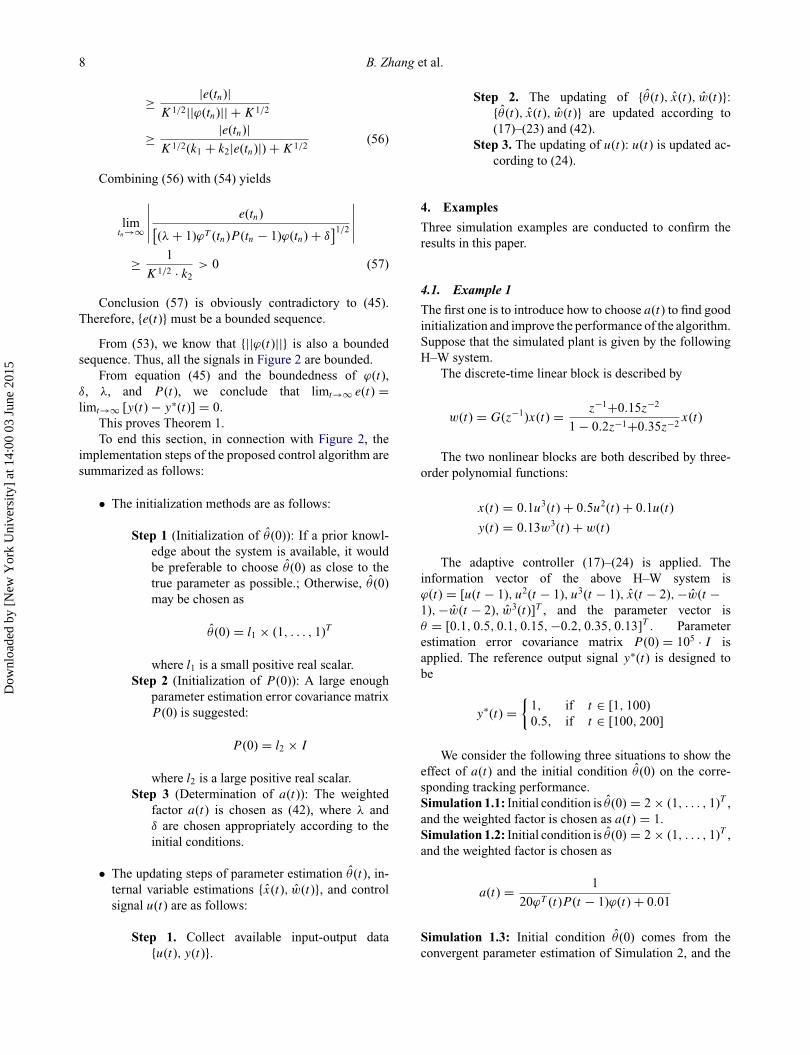
Figure 3. Output response and control input signal in Simulation 1.2.

weighted factor is chosen as

a(t) = 1

10ϕT (t)P (t − 1)ϕ(t) + 0.01

The simulation experiment goes through 200 samples.Numerical results are shown in Figures 3 and 4 with boththe output response y(t) and input control u(t). In eachgroup of figures, the upper one shows the tracking outputresponse y(t) (the solid line) versus the reference y(t) (thedotted line); while the lower one shows the control signalu(t).

In Simulation 1.1, a divergent tracking is obtained(therefore, it is not shown in the figures). The reason isthat, without a weighted factor a(t), a ‘bad’ initial estimateθ (0) cannot ensure the parameter convergence condition(31); therefore, Theorem 1 cannot hold and the closed-loopH–W system is not stable. In Simulation 1.2, the initial es-timate θ (0) is still ‘bad;’ however, since a suitable weightedfactor a(t) is applied to enlarge the parameter convergencedomain (31), the closed-loop system is stable. At the sametime, it can be seen from Figure 3 that the speed of re-sponse is very slow and therefore the controller cannot beput into practice yet. But through Simulation 1.2, we havesome level of knowledge about the unfamiliar system, andtherefore obtain a ‘good’ enough initial condition for laterwork. In Simulation 1.3, the initialization of θ (0) comesdirectly from the convergent parameter estimation of Sim-ulation 1.2, which is ‘good’ enough for the proposed adap-tive controller (17)–(24) to achieve a satisfactory trackingperformance.

Example 1 confirms the results earlier: the adaptiveform a(t) enlarges the attraction domain, enhance perfor-mance of the proposed algorithm and can be chosen suitablyto explore an unfamiliar H–W system, and obtain a ‘good’enough initialization.

It is noted that in (42) the coefficients λ and δ playimportant roles in controller design. In our experiment, thecoefficient δ is set to be 0.01, but it is of great interest tochoose an appropriate λ. If λ is too large, then, althoughthe closed-loop stability is guaranteed, the response is veryslow; on the other hand, if λ is too small, then the overshootand oscillation may be undesirable. Therefore, it is betterto choose the coefficients λ and δ by trial and error.

Simulations 1.2 and 1.3 can be seen as the procedures toput the proposed adaptive controller (17)–(24) into practicewhen an H–W system is unfamiliar to us. Sure enough, ifparameter estimation of an unfamiliar H–W system is pos-sible to be conducted prior to our experiment, the controllerdesign may become much easier and the performance maybecome better as well. The parameter estimation schemesare extensive indeed: one may refer to the existing con-tributions in Section 1; actually, the parameter estimationalgorithm (17)–(23), which is derived by the use of the in-ternal variable estimation, is also effective in identifyingthe H–W system and the corresponding theoretical proofcan be found in Yu, Mao, and Jia (2013).

4.2. Example 2

In this example, we show the performance of the proposedadaptive controller (17)–(24) when there exist disturbance

Dow

nloa

ded

by [

New

Yor

k U

nive

rsity

] at

14:

00 0

3 Ju

ne 2

015

10 B. Zhang et al.

Figure 4. Output response and control input signal in Simulation 1.3.

uncertainties and plant uncertainties. We consider the fol-lowing two situations:Simulation 2.1: Consider the same H–W system as thatin Example 1. The noise works on the output y(t) withSNR = 20db. The controller is the same as that in Sim-

ulation 1.3. In this work, only disturbance uncertainty isconsidered.Simulation 2.2: Based on Simulation 2.1, some plant un-certainties are also added into the H–W system in this sim-ulation. At the 100th sample time, the whole block-oriented

Figure 5. Output response and control input signal in Simulation 2.1.

Dow

nloa

ded

by [

New

Yor

k U

nive

rsity

] at

14:

00 0

3 Ju

ne 2

015

International Journal of Systems Science 11

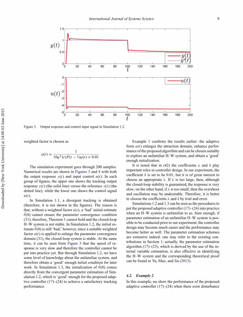
Figure 6. Output response and control input signal in Simulation 2.2.

system suffers about 10% plant uncertainties, i.e., the linearblock becomes

w(t) = G(z−1)x(t) = z−1+0.17z−2

1 − 0.22z−1+0.37z−2x(t)

and the two nonlinear blocks become

x(t) = 0.11u3(t) + 0.52u2(t) + 0.11u(t)

y(t) = 0.15w3(t) + w(t)

The other conditions are the same as those in Simulation2.2. In this work, both disturbance uncertainties and plantuncertainties are considered.

From numerical results shown in Figures 5 and 6, wecan see that the closed-loop tracking performance is satis-factory when uncertainties exist in the nonlinear systems.This confirms that the robustness of the proposed adaptivecontroller is reliable.

4.3. Example 3

In this example, we compare the proposed adaptive con-troller (17)–(24) with some other existing H–W model con-trollers. Consider the following H–W plant:

A smooth saturation is taken as input nonlinearity,which is often encountered in practice:

x(t) = eu(t) − 1

eu(t) + 1

In the state space, the discrete-time linear block is rep-resented by

⎡⎢⎢⎣

�

X1(t + 1)�

X2(t + 1)�

X3(t + 1)

⎤⎥⎥⎦ =

⎡⎣ 2.8 −1.1 0.7

2 0 00 0.5 0

⎤⎦

⎡⎢⎢⎣

�

X1(t)�

X2(t)�

X3(t)

⎤⎥⎥⎦

+⎡⎣−2.5

00

⎤⎦ x(t)

w(t) = [−0.4 0 −0.1]⎡⎢⎢⎣

�

X1(t)�

X2(t)�

X3(t)

⎤⎥⎥⎦

In the above description, we let [�

X1(t),�

X2(t),�

X3(t)]T

be the state. It is sure that the linear block can also bedescribed by the following discrete transfer function:

w(t) = G(z−1)x(t) = z−1 + 0.25z−3

1 − 2.8z−1 + 2.2z−2 − 0.7z−3x(t)

The output nonlinear block is represented by

y(t) = w3(t) + w(t)

The structures of the linear part and the input nonlin-earity of this system are borrowed from Example 4.1 in

Dow

nloa

ded

by [

New

Yor

k U

nive

rsity

] at

14:

00 0

3 Ju

ne 2

015

12 B. Zhang et al.

Figure 7. Output response and control input signal in Simulations 3.1–3.4. (a) Overall view for 100 samples (when the H–W systemsuffers plant parameters uncertainties at the 50th sample, the MPC control scheme via nonlinearities removal utilized in Simulation 3.1leads to divergent and unstable control effect. Thus, this image shows no curves for Simulation 3.1 after the 50th sample.). (b) Partialenlarged details for the 1st to the 30th and the 40th to the 70th samples (the left group of the images shows the dynamic responseperformance, while the right-side group shows the robustness of Simulations 3.2–3.4).

Bloemen et al. (2001) with contrived parameters, which isjust a SISO H model. In order to consider the H–W model,we have also added the output nonlinearity.

In this work, we conduct the following four groups ofexperiments:Simulation 3.1: Apply the model predictive control (MPC)scheme in Patikirikorala et al. (2012) to control the H–Wplant.

This control method is derived from the standard finite-horizon linear MPC scheme. Based on the specific struc-ture of H–W model, the nonlinearities are removed fromthe optimization problem via using pre-inverse and post-inverse nonlinear compensators. Thus, the control problem

in the original nonlinear system is transformed into the in-termediate linear block variables and may be solved using astandard quadratic programming. Some similar approachescan also be found in Fruzzetti et al. (1997), Norquay, Pala-zoglu, and Romagnoli (1998), and Patwardhan, Lakshmi-narayanan, and Shan (1998).Simulation 3.2: Apply the MPC scheme in Bloemen et al.(2001) to control the H–W plant.

This control method is derived from the infinite-horizonrobust MPC scheme, which is first introduced in Kothare,Balakrishnan, and Morari (1996). Unlike the methods inSimulation 3.1, Bloemen et al. (2001) took the effect of theinput and output nonlinearities into account when solving

Dow

nloa

ded

by [

New

Yor

k U

nive

rsity

] at

14:

00 0

3 Ju

ne 2

015

International Journal of Systems Science 13

the optimization problem subject to linear matrix inequal-ities (LMIs). This is achieved by transforming the staticnonlinearities into polytopic descriptions. Thus, the H–Wmodel is represented as a linear model with uncertainty,which enables the use of robust linear MPC techniques tocontrol this kind of system. A similar approach can also befound in Bloemen et al. (2001).Simulation 3.3: Apply the dynamic output feedback MPCscheme (Algorithm 3) in Ding and Ping (2012) to controlthe H–W plant.

This control method is also derived from the infinite-horizon robust MPC scheme. Compared with the earlymethods in Simulation 3.2, some important improvementsare made in Ding and Ping (2012): the state is assumed to beunmeasurable and thus the dynamic output feedback controllaw is derived to satisfy the real industrial situation; somedifferent formulations of the control algorithms with con-siderably lower online computational burden (Ding, Huang,& Xu, 2011) are suggested; the input nonlinearity is allevi-ated by invoking the ‘two-step’ method (Ding & Xi, 2006;Ding, Xi, & Li, 2004). A similar approach can also be foundin Ding and Huang (2007).Simulation 3.4: Apply the proposed adaptive controlscheme to control the H–W plant. We use a five-order poly-nomial function to approximate the input nonlinearity. Theother conditions are the same as those in Examples 1 and2.

In all the experiments, the reference output y∗(t) is al-ways taken to be 2. Let us also introduce the disturbanceξ (t), which is selected to be −0.1 ≤ ξ (t) ≤ 0.1. The dis-turbance works totally on the output nonlinearity, while itmultiplies 0.05 and then works on the linear block.

The simulations go through 100 samples. At the 50thsample, the H–W system suffers the following plant uncer-tainties, i.e., the linear block becomes

⎡⎢⎢⎣

�

X1(t + 1)�

X2(t + 1)�

X3(t + 1)

⎤⎥⎥⎦ =

⎡⎣ 2 −1.1 0.7

1 0 00 0.5 0

⎤⎦

⎡⎢⎢⎣

�

X1(t)�

X2(t)�

X3(t)

⎤⎥⎥⎦

+⎡⎣−2.5

00

⎤⎦ x(t)

w(t) = [−0.4 0 −0.2]⎡⎢⎢⎣

�

X1(t)�

X2(t)�

X3(t)

⎤⎥⎥⎦

or

w(t) = G(z−1)x(t) = z−1+0.25z−3

1 − 2z−1+1.1z−2 − 0.35z−3x(t)

while the two nonlinear blocks remain undisturbed.

Table 1. The computational burdens in Example 3.

Computational time forAlgorithm each iteration (s)

Simulation 3.1 0.01Simulation 3.2 5Simulation 3.3 1.5Simulation 3.4 0.01

Figure 7 shows the output response and control inputsignal in Simulations 3.1–3.4, and Table 1 shows the corre-sponding online computational complexities. It is noted thatsince the MPC control scheme via nonlinearities removalleads to divergent and unstable control effect, we show nocurves for Simulation 3.1 after the 50th sample. To show thedynamic response performance and the robustness clearly,partial enlarged details are also available in Figure 7. Fromthe numerical results, we obtain the following conclusions:

• In Simulation 3.1, since the nonlinearities are directlyremoved from the control problem via an inversion,the effects of the nonlinearities on input–output be-haviors of the plant are not taken into account any-more by the controller. Even though the calculatedx(t) may be optimal with respect to the performanceindex about the intermediate linear block, the result-ing inverted u(t) may be far from the ‘real’ optimalcontrol input. From Figure 7, we find that the over-shoot and oscillation are really severe, which validatethe drawback of simply designing MPC controller vianonlinearities removal. In addition, since the abovecontrol scheme leads to divergent and unstable con-trol effect when plant uncertainties appear at the 50thsample, we know that its robustness is the worst.This conclusion is coincident with the fact that theprimary disadvantage of the commonly used MPCis its inability to deal with plant model uncertainties(Kothare et al., 1996). Meanwhile, the main merit ofthe above controller is that it is easy to be imple-mented and the computational complexity is low.

• In Simulation 3.2, the nonlinearities are transformedinto polytopic descriptions and thus the infinite-horizon MPC algorithm leads to a convex optimiza-tion problem subject to LMIs. From Figure 7, it isshown that the controller offers satisfactory controlperformance. It outperforms the algorithm of Sim-ulation 3.1 mainly because it takes the effect of thenonlinearities into account in the optimization prob-lem. However, at the same time, from Table 1, it isobvious that the computational burden is too heavy.It has become a consensus that the implementation ofthe LMIs-based MPC algorithm suffers from a largecomputational burden due to the complex optimiza-tion problem solved at every sampling time (Ping &

Dow

nloa

ded

by [

New

Yor

k U

nive

rsity

] at

14:

00 0

3 Ju

ne 2

015

14 B. Zhang et al.

Ding, 2013). On the other hand, from the control ef-fect of the later 50 samples when plant uncertaintiessuffered, we find that its robustness is still limited andseems not good enough.

• In Simulation 3.3, since some important improve-ments are made in Ding and Ping (2012), fromFigure 7 and Table 1, it is known that both thecontroller performance (the dynamic response per-formance and the robustness) and the computationaltime are improved. However, due to the inevitable op-timization procedure, it may be still only suitable toimplement such a controller on some slow-responsecontrol systems, e.g., some chemical industry controlsystems.

• In Simulation 3.4, the main merits of the proposedadaptive controller are shown in Figure 7 and Table 1:the closed-loop performance is satisfactory; at thesame time, the controller is suitable to be imple-mented online. In addition, as the proposed controlscheme also contains the recursive estimator, thus thecontroller can adaptively handle the plant uncertain-ties and guarantee the closed-loop stability.

It is also necessary to point out the limitations of theproposed adaptive control scheme at the present stage. Al-though it has already been shown in the simulation studythat, compared with the method in Ding and Ping (2012),the proposed method is simpler, easier to be implementedonline, and more adaptive to plant uncertainties; however,three main drawbacks are as follows:

• For H–W models containing some complex and hardnonlinearities, the descriptions in (3)–(6) may be nomore appropriate, which may lead to unsatisfactorycontrol performance. For instance, the descriptions(3)–(6) may not deal with the nonlinearities in Ex-amples 6.1–6.2 in Ding and Ping (2012).

• From numerical results, the proposed algorithmtracks the reference rapidly; however, it also some-times lead to small overshoot and undershoot at thebeginning procedure. This may be improved by tak-ing the control signal increment into account in thecriterion function (7). It is well known that the adap-tive control scheme derived from such criterion hasalways been a challenge (Lo, Jiang, & Li, 2009), es-pecially for the H–W nonlinear system. Some furtherresearches on this topic are interesting.

• Theoretical results have shown that the closed-loopstability can be guaranteed under sufficient condition(31). At present, we give a qualitative analysis for thissufficient condition and set the weighed factor a(t)as an adaptive form to enhance the stability. How-ever, this treatment may still limit the performanceof the proposed controller. A better choice may besome deeper quantitative analysis of the sufficientcondition (31).

In sum, the proposed control method has some signif-icant merits, but some further researches are still needed.We should also point it out that, for some complex H–Wsystems, the method in Ding and Ping (2012) may result inbetter performance.

5. Conclusions

In this note, an adaptive controller is developed for the H–W systems. In view of adaptive control of H–W systems, anattractive parameterization method is by the key-term sep-aration principle, which is omitted by many researchers.Though the key-term separation principle has been pro-posed several years ago and used to identify the block-oriented models successfully, however, to our knowledge,no general proof of convergence has been carried out. Themain problem of the proof is caused by the presence ofinternal variables in the data vector. In view of this chal-lenge, this work analyzes convergence and stability proper-ties of block-oriented models which are parameterized bythe key-term separation principle. Theoretical results showthat parameter estimation convergence and the closed-loopsystem stability can be guaranteed under sufficient condi-tion. From a qualitative analysis of the sufficient condition,we introduce a weighted factor and set it as an adaptiveform to enhance the stability of the closed-loop system.The basic ideas can be easily extended to adaptively con-trol H and W systems with polynomial nonlinearities. Itis also noted that the key-term separation principle hassuccessfully been used to identify block-oriented modelswith piecewise-linear nonlinearities (Voros, 1999, 2003)or dead-zone nonlinearities (Yu, Mao, & Jia, 2013). Otherproblem areas where further research might give new re-sults are adaptive controllers for these discontinuous block-oriented models.

AcknowledgementsThe authors would like to thank the anonymous reviewers for theirhelpful and constructive comments to improve the quality of thisnote.

FundingThis paper is supported by the National Natural Science Founda-tion of China [grant numbers 61333006, 61473072].

Notes on contributorsBi Zhang was born in Shenyang, Liaon-ing, China. He is currently studying for aPhD degree in the Northeastern University,Shenyang, China. His main research inter-ests are nonlinear adaptive control and pa-rameter estimation.

Dow

nloa

ded

by [

New

Yor

k U

nive

rsity

] at

14:

00 0

3 Ju

ne 2

015

International Journal of Systems Science 15

Hyokchan Hong is working towards hisPhD degree at Northeastern University,China. His main research interests are non-linear system modeling and control.

Zhi-Zhong Mao received his BS degreefrom Harbin Electrician College, Harbin,China in 1982, and the MS and PhD degreesfrom Northeastern University, Shenyang,China in 1984 and 1991 respectively. Heis a professor and a PhD supervisor atNortheastern University, China. His mainresearch interests are modeling, control andoptimization in complex industrial systems.

ReferencesBai, E. (1998). An optimal two-stage identification algorithm for

Hammerstein–Wiener nonlinear systems. Automatica, 34(3),333–338.

Bai, E. (2002). A blind approach to the Hammerstein–Wienermodel identification. Automatica, 38(6), 967–979.

Bloemen, H., Boom, T., & Verbruggen, H. (2001). Model-basedpredictive control for Hammerstein–Wiener systems. Inter-national Journal of Control, 74(5), 482–495.

Bloemen, H., Chou, C., Boom, T., Verdult, V., Verhaegen, M., &Backx, T. (2001). Wiener model identification and predictivecontrol for dual composition control of a distillation column.Journal of Process Control, 11(6), 601–620.

Boutayeb, M., & Aubry, D. (1999). A strong tracking extendedKalman observer for nonlinear discrete-time systems. IEEETransactions on Automatic Control, 44(8), 1550–1556.

Boutayeb, M., & Darouach, M. (1995). Recursive-identificationmethod for MISO Wiener–Hammerstein model. IEEE Trans-actions on Automatic Control, 40(2), 287–291.

Chen, H.F. (2007). Adaptive regulator for Hammerstein andWiener systems with noisy observations. IEEE Transactionson Automatic Control, 52(4), 703–709.

Chen, H.F., & Guo, L. (1991). Identification and stochastic adap-tive control. Boston, MA: Birkhauser.

Ding, B., & Huang, B. (2007). Output feedback model predic-tive control nonlinear systems represented by Hammerstein–Wiener model. IET Control Theory Applications, 1(5), 1302–1310.

Ding, B., Huang, B., & Xu, F. (2011). Dynamic output feedbackrobust model predictive control. International Journal of Sys-tems Science, 42(10), 1669–1682.

Ding, B., & Ping, X. (2012). Dynamic output feedback modelpredictive control for nonlinear systems represented byHammerstein–Wiener model. Journal of Process Control,22(9), 1773–1784.

Ding, B., & Xi, Y. (2006). A two-step predictive control design forinput saturated Hammerstein systems. International Journalof Robust Nonlinear Control, 16(7), 353–367.

Ding, B., Xi, Y., & Li, S. (2004). On the stability of output feedbackpredictive control for systems with input nonlinearity. AsianJournal of Control, 6(3), 388–397.

Ding, F., & Chen, T.W. (2005). Identification of Hammersteinnonlinear ARMAX systems. Automatica, 41(9), 1479–1489.

Ding, F., Chen, T.W., & Iwai, Z. (2007). Adaptive digital con-trol of Hammerstein nonlinear systems with limited output

sampling. SIAM Journal of Control and Optimization, 45(6),2257–2276.

Dolanc, G., & Strmcnik, S. (2008). Design of a nonlinear con-troller based on a piecewise-linear Hammerstein model. Sys-tems & Control Letters, 57(4), 332–339.

Figueroa, J.L., Cousseau, J.E., Werner, S., & Laakso, T. (2007).Adaptive control of a Wiener type system: application of apH neutralization reactor. International Journal of Control,80(2), 231–240.

Fruzzetti, K., Palazoglu, A., & McDonald, K. (1997). Nonlinearmodel predictive control using Hammerstein models. Journalof Process Control, 7(1), 31–41.

Fu, Y., & Chai, T. (2013). Robust regulation of discrete timenonlinear systems with arbitrary nonlinearities. Automatica,49(8), 2567–2570.

Giri, F., & Bai, E. (2010). Block-oriented nonlinear system iden-tification. London: Springer.

Giri, F., Rochdi, Y., & Chaoui, F.Z. (2009). Hammerstein systemidentification in presence of hard nonlinearities of preloadand dead-zone type.IEEE Transactions on Automatic Control,54(9), 2174–2178.

Goodwin, G.C., & Sin, K.S. (1984). Adaptive filtering, predictionand control. Englewood Cliffs, NJ: Prentice-Hall.

Harinischmacher, G., & Marquardt, W. (2007). Nonlinear modelpredictive control of multivariable processes using block-structured models. Control Engineering Practice, 15(10),1238–1256.

Kim, K., Rios-Patron, E., & Braatz, R. (2012). Robust nonlinearinternal model control of stable Wiener systems. Journal ofProcess Control, 22(8), 1468–1477.

Kothare, M., Balakrishnan, V., & Morari, M. (1996). Robust con-strained model predictive control using linear matrix inequal-ities. Automatica, 32(10), 1361–1379.

Kung, M., & Womack, B. (1983). Stability analysis of a discrete-time adaptive control algorithm having a polynomial in-put.IEEE Transactions on Automatic Control, 28(12), 1110–1112.

Liu, Y., & Bai, E. (2007). Iterative identification of Hammersteinsystems. Automatica, 43(2), 346–354.

Ljung, L. (1999). System identification: Theory for the user. En-glewood Cliffs, NJ: Prentice-Hall.

Lo, K., Jiang, R., & Li, D. (2009). Adaptive one-step-ahead op-timal controller based on WLS schemes. International Jour-nal of Adaptive Control and Signal Processing, 23(3), 241–259.

Lv, X., & Ren, V. (2012). Non-iterative identification and modelfollowing control of Hammerstein systems with asymmetricdead-zone nonlinearities. IET Control Theory and Applica-tions, 6(1), 84–89.

Moreno-Valenzuela, J. (2013). Adaptive anti control of chaos forrobot manipulators with experimental evaluations. Communi-cation in Nonlinear Science and Numerical Simulation, 18(1),1–11.

Norquay, S., Palazoglu, A., & Romagnoli, J. (1998). Model predic-tive control based on Wiener models. Chemical EngineeringScience, 53(1), 75–84.

Pajunen, G. (1992). Adaptive control of Wiener type-nonlinearsystems. Automatica, 28(4), 781–785.

Patikirikorala, T., Wang, L., Colman, A., & Han, J. (2012).Hammerstein–Wiener nonlinear model based predictive con-trol for relative QoS performance and resource managementof software systems. Control Engineering Practice, 20(1),49–61.

Patwardhan, R., Lakshminarayanan, S., & Shan, S. (1998). Con-strained nonlinear MPC using Hammerstein and Wiener mod-els: PLS framework. AIChE Journal, 42(7), 1611–1622.

Dow

nloa

ded

by [

New

Yor

k U

nive

rsity

] at

14:

00 0

3 Ju

ne 2

015

16 B. Zhang et al.

Ping, X., & Ding, B. (2013). Off-line approach to dynamic outputfeedback robust model predictive control. Systems & ControlLetters, 62(11), 1038–1048.

Voros, J. (1999). Iterative algorithm for parameter identification ofHammerstein systems with two-segment nonlinearities. IEEETransactions on Automatic Control, 44(11), 2145–2149.

Voros, J. (2003). Modeling and identification of Wiener systemswith two-segment nonlinearities.IEEE Transactions on Con-trol Systems Technology, 11(2), 253–257.

Yu, F., Mao, Z., & Jia, M. (2013). Recursive identification forHammerstein–Wiener systems with dead-zone input nonlin-earity. Journal of Process Control, 23(8), 1108–1115.

Zhao, W., & Chen, H. (2009). Adaptive tracking and recursiveidentification for Hammerstein systems. Automatica, 45(12),2773–2783.

Zhu, Y. (2002). Estimation of an N-L-N Hammerstein–Wienermodel. Automatica, 38(9), 1607–1614.

Dow

nloa

ded

by [

New

Yor

k U

nive

rsity

] at

14:

00 0

3 Ju

ne 2

015