IAA-AAS-DyCoSS2-14 -02-01

AUTONOMOUS GUIDANCE AND CONTROL IN THE PROXIMITYOF ASTEROIDS USING A SIMPLE MODEL OF THE

GRAVITATIONAL POTENTIAL

Andrea Turconi∗, Phil Palmer†, and Mark Roberts‡

Proximity operations about asteroids are challenging because of the small and non-uniform attraction of those celestial bodies. In addition, the combination of suchgravitational potentials with the asteroids’ rotation, generates equilibrium pointsaround them. In order to perform autonomous guidance, a spacecraft will needa model of the gravitational potential that can be handled on-board besides theknowledge of the asteroid’s rotation and of relative position and velocity. Thiswork describes guidance laws that, thanks to a simplified gravity model, take ad-vantage of the natural dynamics in proximity of asteroids and of the properties oftheir equilibrium points.

INTRODUCTION

Asteroids are the next destination of space exploration as they represent an unparalleled historicalarchive which is fundamental for our understanding of the formation of the Solar System. They arelocated mainly in the Asteroid Belt, between 2 to 3.5AU and in the stable points of the Sun-Jupitersystem, but some of them orbit in the inner Solar System and can come closer to the Earth posinga threat to our home planet. In order to mitigate the risk of dangerous close encounters we need tofind and study them for developing planetary defence strategies.Another interesting aspect is that some of these small bodies turn out to be even more accessible thanthe Moon in terms of deltaV requirements. For this reason Near Earth Asteroids have become thenatural targets for the first manned missions venturing outside the Earth-Moon system in preparationfor the exploration of Mars. Small bodies also represent deposits of raw materials already floatingin space, especially rare metals and water ice, these can be possibly used to foster future explorationand human presence in the Solar System.

In order to fulfil any of the previous objectives it is required to send spacecraft capable to ma-noeuvre in the vicinity of asteroids. In the past two decades many milestones have been achieved,from the first flybys (Galileo, NASA/ESA, 1991) to missions featuring stable orbits and eventuallylanding on the surface (NEAR-Shoemaker, NASA, 2000) or even getting dust samples back to theEarth (Hayabusa, JAXA, 2005). However, proximity operations — with the exceptions of the termi-nal legs of landing trajectories — have always been performed with a ground-in-the-loop approach.

∗Ph.D. Student (ESR in AstroNet-II Marie-Curie ITN), Surrey Space Centre, University of Surrey, Guildford, England,GU2 7XH, United Kingdom, a.turconi@surrey.ac.uk†Professor, Surrey Space Centre, University of Surrey, Guildford, England, GU2 7XH, United Kingdom,p.palmer@surrey.ac.uk‡Professor, Department of Mathematics, University of Surrey, Guildford, GU2 7XH, United Kingdom,m.roberts@surrey.ac.uk

1

This implies that extensive use of ground station time is required to carry through the mission witha substantial impact in overall costs. Moreover, with all the knowledge about the orbital dynamicsof the spacecraft being on the ground, the operations rely on preplanned commands and missionprofiles are constrained by communications delays.

The technology for autonomous navigation in the vicinity of asteroids is already available. Whatis missing is a way of modelling on-board the non-uniform gravitational potential of these smallbodies and a guidance and control strategy that can rely on such inherently simple and approximategravitational models.

In this paper we review, at first, the current approach and models used for operating spacecraftabout asteroids. We then describe the dynamical environment in the vicinity of small bodies focus-ing on those features that can be exploited for autonomous guidance purposes. Finally we presenta control strategy to negotiate the spacecraft to a synchronous orbit about the asteroid and its be-haviour thanks to simulations results.

BACKGROUND

The irregular shape of asteroids creates an inhomogeneous gravitational field in which the space-craft generally moves along non-closed and unstable trajectories. In order to guide a spacecraftin the vicinity of an asteroid, elementary characteristics of the small body need to be determined:shape, mass and spin rate.Under favourable conditions, it is possible to have an idea of those quantities from the ground, es-pecially when dealing with bigger asteroids. For most of the bodies it is possible to perform albedoand light-curve analysis1, 2 and, in case of close encounters with the Earth, good shape models areobtained via radar imaging.3

However, most of the times, the accuracy of these data has to be significantly improved in order tocarry out the mission successfully.

Much of the detailed characterisation work is therefore based on in-situ observations.Mass is estimated thanks to flybys taking place before orbit insertion. Imaging the asteroid undervarious lighting condition enables the construction of a shape model and the determination of thespin rate.4, 5 Knowing the mass and the shape, a density estimate is derived. Using this model ofa spinning shape with constant density, trajectory analysis for the following phases of the missioncan be performed. Further perturbations that may be detected are used to refine the model. Abetter representation of the gravitational potential yields a more accurate prediction of the spacecrafttrajectory and enables the ground controllers to safely guide the satellite at lower altitudes above thesurface.

All these steps of characterisation actually rely on the measurement of relative position and ve-locity between the spacecraft and the asteroid. These measurements are the result of Range-Dopplercampaigns accomplished using the huge antennas of the Deep Space Network (DSN).6 A polyhe-dral shape model7 is created thanks to high-resolution images8 and LIDAR measurements, com-bined with the trajectory of the spacecraft measured from the ground. The models of the asteroidare assembled on the ground as well, so the satellite has no knowledge of the dynamical environ-ment in which it is immersed, and it simply executes, at prescribed times, manoeuvring commandspreviously prepared on the ground. Given the delay in communications caused by the distance be-tween the spacecraft and the Earth, everything has to be carefully planned in advance and constantlymonitored.

2

In recent years the developments of the AutoNav software and in particular of its OBIRON com-ponent (On-board Image Registration and Optical Navigation) has demonstrated the feasibility ofautonomous optical navigation in proximity of asteroids.5 In this work we assume that an Opti-cal Navigation software like OBIRON is available on the spacecraft providing relative position andvelocity with respect to the asteroid centre of mass.

To enable autonomous guidance in the proximity of asteroids is required a model of the gravi-tational potential than can be used on-board. The limited computational resources available on thespacecraft suggest that it is impractical to use the detailed polyhedral models for this task. Thereforewe have to choose a class of approximate models of the gravitational potential that, although notglobally accurate, can still represent well some dynamical characteristics that can be useful for theautonomous guidance laws. For our purpose we will use the 3-spheres model developed recently atthe Surrey Space Centre9 which is able to represent with good accuracy the position, the dynamicalbehaviour and the energy level of the equilibrium points of the asteroid.10

ASTEROID ROTATION AND EQUILIBRIUM POINTS

The majority of asteroids are in a stable rotation about the axis of their biggest moment of inertiawith periods of some hours. Fast rotators and tumbling asteroids exist, but they are not predomi-nant11 therefore we will consider the small body to be in uniform rotation.

Equations of motion in the body fixed frame

A reference frame fixed with the asteroid is used to describe the motion of the spacecraft relativeto the rotating body. In such a reference frame the gravitational potential will not vary with time.We will call this reference frame Body Centred Body Fixed abbreviated, as BCBF.If we define a principal axis reference frame x, y, z such that the principal moments of inertia will beIzz > Iyy > Ixx, because of the rotation along the biggest moment of inertia, it will be convenientto place the z-axis of the reference frame in the direction of the angular velocity vector ω, as shownin Figure 1.

x

y

z

ω

aG

aCFaCO r

.

r

Figure 1. Body Centred Body Fixed (BCBF) reference frame. x, y and z are principalaxis of inertia and ω is a uniform rotation vector in the same direction of z. r and rrepresent position and velocity of the spacecraft relative to the asteroid while aG, aCF,aCO are the gravitational, centrifugal and Coriolis accelerations.

In such a non-inertial frame the fictitious terms of the accelerations due to the uniform rotation

3

of the reference frame will appear. The total acceleration r in the BCBF frame is given by thecombination of the gravitational, centrifugal and Coriolis accelerations — respectively aG, aCF

and aCO — as shown in Equation 1. Position, velocity and acceleration in the BCBF frame arerepresented by r, r, r, ω is the rotation rate vector and U the gravitational potential of the asteroidwhich is time invariant in the BCBF rotating frame and therefore depends only on the position r.

r = aG + aCF + aCO + aEU

aG = ∇UaCF = −ω × (ω × r)

aCO = −2ω × r

(1)

As shown in Figure 1 the centrifugal acceleration points always in the radial direction, the Coriolisacceleration is always perpendicular to the velocity vector imparting to it a clockwise rotation,and finally the gravitational acceleration is in general not directed radially due to the non-uniformgravitational potential.

Equilibrium points

For most of the asteroids there will be equilibrium points. By setting r and r to zero in Equation1 we find that these are the points where the gravitational pull balances the centrifugal force.

aG = −aCF (2)

x

y

z

ω

*

*

*

*

Figure 2. Equilibrium points given by the balance between gravitational and cen-trifugal accelerations in the BCBF frame rotating with the asteroid are shown as redstars

Uniformly rotating asteroids have generally 4 equilibrium points placed roughly along the shortand long axes of the body and lying in the equatorial plane12 as shown in Figure 2. These equi-librium points are fixed in the BCBF frame in the same way as the Lagrange Points are fixed in

4

the synodic frame of the Circular Restricted 3-body Problem (CR3BP).13 As the Lagrange points,the asteroids’ equilibrium points feature various dynamical behaviours depending on the sign of thesecond derivatives of the gravitational potential evaluated there.

Writing Equation 1 in the equatorial plane we find the equations of motion in cartesian and polarcomponents: Equations 3 and 4

x =∂U

∂x+ 2ωy + ω2x

y =∂U

∂y− 2ωx+ ω2y

(3)

r =

∂U

∂r+ 2ωrθ + ω2r

rθ =1

r

∂U

∂θ− 2ωr

(4)

Setting the velocity and the total acceleration to zero, Equations 5 and 6 express the conditionto be verified at the equilibrium points. In Equation 6 is made clear that at the equilibrium pointsthe tangential component of the gradient of the potential shall be zero by itself since it cannot bebalanced by the centrifugal acceleration.

−ω2x =∂U

∂x

−ω2y =∂U

∂y

(5)

−ω2r =

∂U

∂r

0 =∂U

∂θ

(6)

The positions of the equilibrium points have been computed solving numerically the system ofnon-linear equations shown in Equation 5.

The Jacobi Energy Integral

One of the biggest challenges in performing proximity operations is that, in general, low orbitsabout small bodies are unstable and lead either to impact the asteroid or to escape its sphere ofinfluence and then drift in deep space.

As it happens in the CR3BP, for any uniformly rotating gravitational potential, a constant ofmotion exists in the rotating frame. Such a conserved quantity is called Jacobi Integral of Motionor, more simply, Jacobi Energy. It is computed as shown in Equation 7 by adding the centrifugalpotential to the expression of the total mechanical energy:

J(r, r) =1

2|r|2 − U(r)− 1

2|ω|2|r|2 (7)

where J is the Jacobi Energy, r is the velocity vector in the body fixed frame,U is the gravitationalpotential, ω is angular rate of the small body and r is the position vector in the body fixed frame.

5

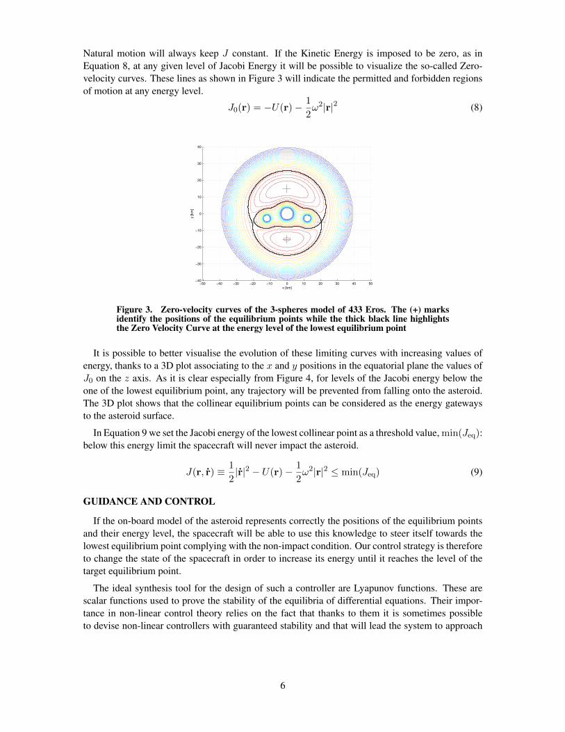
Natural motion will always keep J constant. If the Kinetic Energy is imposed to be zero, as inEquation 8, at any given level of Jacobi Energy it will be possible to visualize the so-called Zero-velocity curves. These lines as shown in Figure 3 will indicate the permitted and forbidden regionsof motion at any energy level.

J0(r) = −U(r)− 1

2ω2|r|2 (8)

−50 −40 −30 −20 −10 0 10 20 30 40 50−40

−30

−20

−10

0

10

20

30

40

x [km]

y [km

]

Figure 3. Zero-velocity curves of the 3-spheres model of 433 Eros. The (+) marksidentify the positions of the equilibrium points while the thick black line highlightsthe Zero Velocity Curve at the energy level of the lowest equilibrium point

It is possible to better visualise the evolution of these limiting curves with increasing values ofenergy, thanks to a 3D plot associating to the x and y positions in the equatorial plane the values ofJ0 on the z axis. As it is clear especially from Figure 4, for levels of the Jacobi energy below theone of the lowest equilibrium point, any trajectory will be prevented from falling onto the asteroid.The 3D plot shows that the collinear equilibrium points can be considered as the energy gatewaysto the asteroid surface.

In Equation 9 we set the Jacobi energy of the lowest collinear point as a threshold value, min(Jeq):below this energy limit the spacecraft will never impact the asteroid.

J(r, r) ≡ 1

2|r|2 − U(r)− 1

2ω2|r|2 ≤ min(Jeq) (9)

GUIDANCE AND CONTROL

If the on-board model of the asteroid represents correctly the positions of the equilibrium pointsand their energy level, the spacecraft will be able to use this knowledge to steer itself towards thelowest equilibrium point complying with the non-impact condition. Our control strategy is thereforeto change the state of the spacecraft in order to increase its energy until it reaches the level of thetarget equilibrium point.

The ideal synthesis tool for the design of such a controller are Lyapunov functions. These arescalar functions used to prove the stability of the equilibria of differential equations. Their impor-tance in non-linear control theory relies on the fact that thanks to them it is sometimes possibleto devise non-linear controllers with guaranteed stability and that will lead the system to approach

6

Figure 4. Zero-velocity surface of the 3-spheres model of 433 Eros. The black dashedline highlights the Zero Velocity Curve at the energy level of the lowest equilibriumpoint

the set point asymptotically never exceeding it. A Lyapunov function shall be positive definite andits derivative shall always be negative for values other than zero. Equation 10 summarizes thoseconditions:

V : Rn → R ; V (0) = 0 ; V (J) > 0 ; V (J 6= J∗) < 0 (10)

We have chosen as Lyapunov function V = 12(J∗ − J)2, with J Jacobi Energy and J∗ target

Jacobi Energy such that J∗ = min(Jeq). The derivative of this Lyapunov function is:

V = −(J∗ − J)dJdt

withdJ

dt= xx+ yy = aCTRL · r

(11)

where J is the Jacobi energy, J∗ the target Jacobi energy, r the velocity vector and aCTRL thecontrol acceleration. Equation 11 tells us that the energy will change only because of the componentof the control acceleration that modifies the magnitude of the velocity.

In order to ensure that the derivative of the Lyapunov function will always be negative, it isrequired an appropriate expression for the control acceleration. Our choice is shown in Equation 12

aJ =|ω||r|

(J∗ − J) r

|r|(12)

7

An integrator using the Bulirsch-Stoer method has been developed for the propagation of theequations of motion in the rotating frame. The code has been validated by integrating free motiontrajectories and verifying the conservation of the Jacobi Energy. In this propagator has been addedthe computation of the proposed control acceleration and simulations have been performed.An example of the results that can be obtained with this control law is shown in Figures 5, 6 and7. As we expect the value of J quickly approaches the target. From that moment onwards thespacecraft moves in free motion with constant energy at the level of the target equilibrium point. Atthat point the control law is inactive because the target energy has been reached and the differencein energy has become zero.

0 1 2 3 4 5−70

−65

−60

−55

Periods [−]

Ja

co

bi E

ne

rgy [

m2 s

−2]

Jacobi Energy [m2 s

−2]

J*

J

J0

0 1 2 3 4 5

0

10

20

x 10−5

Periods [−]

aJ [

m s

−2]

Control Acceleration Parallel to the Velocity

aJ

Figure 5. Values of Jacobi Energy and Control Acceleration for the spacecraft con-trolled with the proposed Lyapunov function control law.

Controlling towards the equilibrium point

It has been shown how a Lyapunov control law is able to bring the spacecraft to the correctenergy level. However, the final aim of our guidance is in fact to steer the spacecraft towards thevery equilibrium point. To do so we need to add another term to the acceleration, a term that shallincorporate the information of the position of the equilibrium point or of its direction relative to thespacecraft.

With this additional component of the control acceleration we don’t want to affect the energy,this implies that the new acceleration has to be always normal to the velocity, so that the derivativeof the Jacobi Energy is always zero as in Equation 13

dJ

dt= a⊥ · r = 0 (13)

Since we want to steer the spacecraft towards the target equilibrium point we will use the angle

8

0 1 2 3 4 50

100

200

Periods [−]

Ra

diu

s [

km

] Radius

r*

r

0 1 2 3 4 5

−pi−pi/2

0pi/2

pi

Periods [−]

Th

eta

[ra

d]

Theta

θ*

θ

0 1 2 3 4 5−50

0

50

Periods [−]

Ve

locity [

m/s

] Velocity

v

vr

vt

Figure 6. Radius, Polar coordinate θ and and Velocity of the spacecraft controlledwith the proposed Lyapunov function control law. It is interesting to notice how thespacecraft, then in free motion, comes close to the the Zero Velocity Surface as a resultof the natural Coriolis acceleration

−100 −50 0 50 100−100

−80

−60

−40

−20

0

20

40

60

80

100

x [km]

y [

km

]

Trajectory in the rotating frame

Figure 7. Trajectory of a spacecraft controlled with the proposed Lyapunov functionrespecting the non-impact condition. At the target energy the spacecraft could at mosttouch the red zero-velocity curve but it cannot cross it.

9

δ between direction of the target, as seen by the spacecraft, and the the velocity vector as shown inFigures 8 and 9.

x

y

z

ω

*

*

a⟂aCO

r.r

(r*-r)r*

δ

*

.

Figure 8. Geometry of the control acceleration normal to the velocity for δ > 0

x

y

z

ω

*

*

a⟂

aCO

r

(r*-r)r*

r. -δ

Figure 9. Geometry of the control acceleration normal to the velocity for δ < 0

For this component of the acceleration in charge of the rotation of the velocity towards the tar-get, the idea is to design a controller proportional to δ. The intended behaviour is described bya⊥DESIRED in Equation 14 where k⊥ is an adjustable gain always greater than zero.

a⊥DESIRED = k⊥δ|ω||r|

aCO

|aCO|(14)

In the direction normal to the velocity is always present the Coriolis acceleration which continu-ously exerts a rotation towards the right-hand side. It is sensible to take this into account since, forδ > 0, aCO is the same direction of a⊥DESIRED while for δ < 0 it happens to be in the oppositeone. Thinking of the desired behaviour as the result of the combined effect of the control acceler-ation a⊥ and the Coriolis acceleration aCO, we will write Equation 15 and subsequently find theexpression of the control acceleration we where looking for, shown in Equation 16.

a⊥DESIRED = aCO + a⊥ (15)

a⊥ = k⊥δ|ω||r|

aCO

|aCO|− aCO (16)

10

Looking more carefully at Equation 16 we notice that various settings of the gain k⊥ simplyimply that the control acceleration a⊥ will be zero at a specific value of δ or, conversely, that,a⊥DESIRED = aCO rendering the control not necessary. We called δ0 this value of δ where thecontrol action is equal to the natural rotation provided by the Coriolis acceleration. Equation 17relates the value of k⊥ to δ0.

k⊥ =2

δ0(17)

Meaningful values of δ0 range from δ0 = 0→ k⊥ =∞ to δ0 = π → k⊥ = 2/π. For high valuesof δ0 the perpendicular control law may be too slow to rotate the velocity towards the target causingnon-converging behaviour; on the other hand if δ0 is small k⊥ becomes large and the control normalto the velocity is more “nervous” resulting in larger deltaV despite a very fast convergence.

Applying both the components parallel and normal to the velocity, we obtained a guidance lawthat succeeds in matching the prescribed energy level and it is also able to steer the spacecraft tothe target equilibrium point. Results for two different initial conditions are shown in the followingplots. Both the simulations have been computed with δ0 = π/4 and then k⊥ = 8

π .

The first simulation, Figures 10 to 14, has initial conditions r0 = 84 km, θ0 = π/4. The secondsimulation, Figures 15 to 19, has initial conditions r0 = 84 km, θ0 = π.

0 0.5 1 1.5 2 2.5 3−70

−65

−60

−55

Periods [−]

Ja

co

bi E

ne

rgy [

m2 s

−2]

Jacobi Energy [m2 s

−2]

J*

J

J0

0 0.5 1 1.5 2 2.5 3

0

1

2

x 10−4

Periods [−]

aJ [

m s

−2]

Control Acceleration Parallel to the Velocity

aJ

Figure 10. Values of Jacobi Energy and control acceleration parallel to the velocity forthe spacecraft controlled with the complete control law. Initial conditions r0 = 84 km,θ0 = π/4.

11

0 0.5 1 1.5 2 2.5 3

−pi/2

−pi/4

0

pi/4

pi/2

Periods [−]

de

lta

[d

eg

]

Angle Delta [deg]

0 0.5 1 1.5 2 2.5 3−5

0

5

10

15x 10

−3

Periods [−]

ap

erp

[m

s−

2]

Control Acceleration Normal to the Velocity [m s−2

]

Figure 11. Values of δ and control acceleration normal to the velocity for thespacecraft controlled with the complete control law. Initial conditions r0 = 84 km,θ0 = π/4.

0 0.5 1 1.5 2 2.5 30

50

100

Periods [−]

Ra

diu

s [

km

] Radius

r*

r

0 0.5 1 1.5 2 2.5 3

0

Periods [−]

Th

eta

[ra

d]

Theta

θ*

θ

0 0.5 1 1.5 2 2.5 3−50

0

50

Periods [−]

Ve

locity [

m/s

] Velocity

v

vr

vt

Figure 12. Radius, Polar coordinate θ and and Velocity of the spacecraft controlledwith the the complete control law. Initial conditions r0 = 84 km, θ0 = π/4.

12

−20 0 20 40 60 80

−30

−20

−10

0

10

20

30

40

50

60

x [km]

y [

km

]

Trajectory in the rotating frame

Figure 13. Trajectory of the spacecraft controlled with the complete control acceler-ation. Initial conditions r0 = 84 km, θ0 = π/4.

0 1 2 30

0.1

0.2

Periods [−]

de

lta

V [

m/s

]

deltaV

0 1 2 30

2

4x 10

−3

Periods [−]

de

lta

V [

m/s

]

deltaV aJ

0 1 2 30

0.1

0.2

Periods [−]

de

lta

V [

m/s

]

deltaV aperp

0 1 2 30

20

40

Periods [−]

de

lta

V [

m/s

]

Cumulative deltaV

0 1 2 30

2

4

Periods [−]

de

lta

V [

m/s

]

Cumulative deltaV aJ

0 1 2 30

20

40

Periods [−]

de

lta

V [

m/s

]

Cumulative deltaV aperp

Figure 14. deltaV expended, total and by the parallel and normal component, usingthe complete control acceleration. Initial conditions r0 = 84 km, θ0 = π/4.

13

0 0.5 1 1.5 2 2.5 3

−70

−65

−60

−55

Periods [−]

Ja

co

bi E

ne

rgy [

m2 s

−2]

Jacobi Energy [m2 s

−2]

J*

J

J0

0 0.5 1 1.5 2 2.5 3

0

10

20

x 10−5

Periods [−]

aJ [

m s

−2]

Control Acceleration Parallel to the Velocity

aJ

Figure 15. Values of Jacobi Energy and control acceleration parallel to the velocity forthe spacecraft controlled with the complete control law. Initial conditions r0 = 84 km,θ0 = π.

0 0.5 1 1.5 2 2.5 3

−pi/2

−pi/4

0

pi/4

pi/2

Periods [−]

de

lta

[d

eg

]

Angle Delta [deg]

0 0.5 1 1.5 2 2.5 3−0.01

0

0.01

0.02

Periods [−]

ap

erp

[m

s−

2]

Control Acceleration Normal to the Velocity [m s−2

]

Figure 16. Values of δ and control acceleration normal to the velocity for the space-craft controlled with the complete control law. Initial conditions r0 = 84 km, θ0 = π.

14

0 0.5 1 1.5 2 2.5 30

50

100

Periods [−]

Ra

diu

s [

km

] Radius

r*

r

0 0.5 1 1.5 2 2.5 3

−pi−pi/2

0pi/2

pi

Periods [−]

Th

eta

[ra

d]

Theta

θ*

θ

0 0.5 1 1.5 2 2.5 3−50

0

50

Periods [−]

Ve

locity [

m/s

] Velocity

v

vr

vt

Figure 17. Radius, Polar coordinate θ and and Velocity of the spacecraft controlledwith the the complete control law. Initial conditions r0 = 84 km, θ0 = π.

−80 −60 −40 −20 0 20

−40

−30

−20

−10

0

10

20

30

40

50

x [km]

y [

km

]

Trajectory in the rotating frame

Figure 18. Trajectory of the spacecraft controlled with the complete control acceler-ation. Initial conditions r0 = 84 km, θ0 = π.

15

0 1 2 30

0.1

0.2

Periods [−]

de

lta

V [

m/s

]

deltaV

0 1 2 30

2

4x 10

−3

Periods [−]

de

lta

V [

m/s

]

deltaV aJ

0 1 2 30

0.1

0.2

Periods [−]

de

lta

V [

m/s

]

deltaV aperp

0 1 2 30

50

Periods [−]

de

lta

V [

m/s

]

Cumulative deltaV

0 1 2 30

1

2

Periods [−]

de

lta

V [

m/s

]

Cumulative deltaV aJ

0 1 2 30

50

Periods [−]

de

lta

V [

m/s

]

Cumulative deltaV aperp

Figure 19. deltaV expended, total and by the parallel and normal component, usingthe complete control acceleration. Initial conditions r0 = 84 km, θ0 = π.

CONCLUSIONS AND FUTURE WORK

From the analysis of the dynamical environment about a rotating asteroid we have designed con-trol laws that are capable to guide a spacecraft to the equilibrium point at the lowest energy in thevicinity of the small body. To do so we used a very simple model of the gravitational potentialalready known to be a viable solution for a good representation of the position and energy level ofthe equilibrium points. Such a strategy can be performed autonomously by a spacecraft in orbit,provided that the approximate model is present on-board and an Optical Navigation package is ableto estimate relative distance and relative velocity throughout the control phase.

Further developments of this concept will include a testing phase performed by propagating thetrajectory of the spacecraft about a truth model of the asteroid, while the controller will continue touse the simplified model. Then we plan to develop an algorithm for generating 3-spheres (or 3 pointmass) models of asteroids. We will take as input the shape models which are likely to be created inthe early phases of missions in order to enable the autonomous optical navigation.

ACKNOWLEDGEMENT

This research has been funded by the European Commission through the Marie Curie InitialTraining Network PITN-GA-2011-289240, ”AstroNet-II The Astrodynamics Network”

REFERENCES

[1] J. Torppa, M. Kaasalainen, T. Michaowski, T. Kwiatkowski, A. Kryszczyska, P. Denchev, and R. Kowal-ski, “Shapes and rotational properties of thirty asteroids from photometric data,” Icarus, Vol. 164, Aug.2003, pp. 346–383, 10.1016/S0019-1035(03)00146-5.

16

[2] B. Carry, M. Kaasalainen, and W. Merline, “Shape modeling technique KOALA validated by ESARosetta at (21) Lutetia,” Planetary and Space Science, No. 66(1), 2012, pp. 200–212.

[3] R. S. Hudson and S. J. Ostro, “Shape of Asteroid 4769 Castalia (1989 PB) from Inversion of RadarImages.,” Science (New York, N.Y.), Vol. 263, Feb. 1994, pp. 940–3, 10.1126/science.263.5149.940.

[4] J. Miller, A. S. Konopliv, P. G. Antreasian, J. J. Bordi, S. Chesley, C. E. Helfrich, W. M. Owen, T. C.Wang, B. G. Williams, D. K. Yeomans, and D. J. Scheeres, “Determination of Shape, Gravity, andRotational State of Asteroid 433 Eros,” Icarus, Vol. 155, No. 1, 2002, pp. 3–17, 10.1006/icar.2001.6753.

[5] S. Bhaskaran, S. Nandi, and S. Broschart, “Small Body Landings Using Autonomous Onboard OpticalNavigation,” The Journal of the Astronautical Sciences, Vol. 58, Mar. 2011, pp. 409–427.

[6] D. Yeomans, P. Antreasian, and J. Barriot, “Radio science results during the NEAR-Shoemaker space-craft rendezvous with Eros,” Science, Vol. 289, Sept. 2000, pp. 2085–8.

[7] R. Werner and D. Scheeres, “Exterior gravitation of a polyhedron derived and compared with harmonicand mascon gravitation representations of asteroid 4769 Castalia,” Celestial Mechanics and DynamicalAstronomy, 1996.

[8] R. W. Gaskell, O. S. Barnouin-Jha, D. J. Scheeres, a. S. Konopliv, T. Mukai, S. Abe, J. Saito, M. Ishig-uro, T. Kubota, T. Hashimoto, J. Kawaguchi, M. Yoshikawa, K. Shirakawa, T. Kominato, N. Hirata, andH. Demura, “Characterizing and navigating small bodies with imaging data,” Meteoritics & PlanetaryScience, Vol. 43, June 2008, pp. 1049–1061.

[9] E. Herrera-Sucarrat, P. L. Palmer, and R. M. Roberts, “Modeling the Gravitational Potential of a Non-spherical Asteroid,” Journal of Guidance, Control, and Dynamics, Vol. 36, May 2013, pp. 790–798.

[10] E. H. Sucarrat, The Full Problem of Two and Three Bodies : Application to Asteroids and Binaries.PhD thesis, University of Surrey, 2012.

[11] P. Pravec, A. Harris, and T. Michalowski, “Asteroid rotations,” Asteroids III, 2002, pp. 113–122.[12] D. J. Scheeres, Orbital Motion in Strongly Perturbed Environments: Applications to Asteroids, Comet

and Planetary Satellite Orbiters. London, UK: Springer-Praxis, 2012.[13] D. Vallado, Fundamentals of astrodynamics and applications. Microcosm Press, Springer, 2007.

17