1

EXAMINING THE PROPERTIES OF THE WATERBED EFFECT IN SPACECRAFT DISTURBANCE REJECTION CONTROL SYSTEMS*

Edwin S. Ahn,† Richard W. Longman,‡ and Richard Carreras §

Spacecraft have mechanical rotating devices onboard such as CMG’s, reaction wheels, cryo pumps, etc. Slight imbalances within these rotating devices cause structural vibrations or jitter, affecting fine pointing equipment. Examples in-clude use of laser communication between spacecraft over a long distance. Re-petitive control and various adaptive algorithms can address periodic disturb-ance with a fundamental and harmonics. Linear feedback control systems are subject to the waterbed effect that says if disturbances are attenuated in some frequency range, they must be amplified in some other range. This paper seeks methods of avoiding substantial amplification between addressed frequencies, while keeping the notch width relatively wide for robustness to period uncertain-ty. And in addition, we seeks to find ways that can push the amplification to high frequencies where disturbances are small, as is done in routine feedback control systems. Within repetitive control (RC), no method was found to achieve this last objective, but a zero-phase frequency-dependent RC gain was devel-oped that can assist in performing the compromise between the other two objec-tives. It can produce local modifications of the waterbed behavior. Nonlinear adaptive algorithms are also studied. Although the waterbed theory does not consider nonlinear systems, it is observed that they too are subject to the same kind of limitation. It is also observed that for a complex disturbance environ-ment, adaptive control can shift amplification to high frequencies. Furthermore, the benefits of this shift can be increased by using a faster sample rate.

INTRODUCTION

The attitude control systems for satellites usually use moment exchange devices such as three reaction wheels or 4 control moment gyros (CMG). Cryogenic pumps are also sometimes needed for sensing devices. If the wheels or mechanisms involved are not perfectly balanced, they pro-duce a vibration of the spacecraft structure. This vibration, also known as jitter, can adversely affect the performance of fine pointing equipment, or of the attitude. Extreme examples of the need for high precision pointing include the Hubble Space Telescope whose design objective was to maintain pointing to within 5 thousandths of an arc second accuracy. A new and particularly challenging application is LaserCom. The objective is to produce ultra high bandwidth in com- * The views expressed are those of the author and do not reflect the official policy or position of the US Air Force, De-partment of Defense or the US Government. † NRC Post Doctorate Research Associate, Air Force Research Laboratories, Kirtland AFB, Albuquerque, NM, 87116 ‡ Corresponding Author, Professor of Mechanical Engineering and Civil Engineering, Columbia University MC4703 § Principal Investigator, Air Force Research Laboratories, Kirtland AFB, Albuquerque, NM, 87116

IAA-AAS-DYCOSS2-14-10

2

munication over long distances, by replacing the usual antenna by a laser. This, for example, could allow high definition images transmitted from Mars to earth in real time. NASA studied the development of this technology with experiments aboard the LADEE spacecraft that achieved a download rate of 622 megabits per second. Experiments aboard the ISS are planned with the Op-tical Payload for LaserCom Science (OPALS).

The period of the vibration disturbances can be known, and will consist of a fundamental fre-quency and harmonics. This paper discusses properties of control systems that are designed to eliminate the effects of the jitter at the location of the fine pointing equipment, or the effects of the jitter on the laser beam, eliminating these specific frequencies from the output error. In this case the laser is directed to the receiver using a fast steering mirror (FSM), and the control system is to learn how to move the pan and tilt angles of this mirror to keep the beam directed to the re-ceiver, in spite of the fact that the mirror is mounted on a structure that has jitter. In this paper some methods are studied in a general context, and others consider the specific application to the LaserCom problem which the authors and others have studied experimentally in References 1-3.

Linear feedback control systems are subject to the Bode Integral Theorem usually referred to as the waterbed effect (Reference 4, 5). For unity feedback control systems, this effect is a prop-erty of the transfer function from the disturbance to a control system to the resulting error, i.e. the sensitivity transfer function (the same transfer function applies from command to tracking error). The disturbance can appear anywhere around the feedback loop, but the theorem considers the equivalent disturbance added to the output of the plant. Consider digital control systems with a frequency range from zero to Nyquist frequency. The usual situation is that, if a linear feedback control system attenuates the error in some frequency range produced by a disturbance input, then it must amplify the error associated with disturbances in some other frequency range. One might ask, why can linear feedback control work in practice? It only works if you attenuate the effects of the disturbances at frequencies where there is substantial error, and you amplify at frequencies where the disturbances are small.

The waterbed effect is actually more dramatic than presented above, because the usual situa-tion is that the log of the error magnitude over the full frequency range must average to zero. Simple thinking says if somehow the error from zero to one half Nyquist were attenuated by a factor of 10, then the error from one half Nyquist to Nyquist must be amplified by a factor of 10. If the disturbance had the same amplitude at all frequencies, then a feedback control system would make the overall error much worse than no control system at all. An example of such a situation is discussed related to a particle accelerator is given in Reference 6.

The sensitivity transfer function for typical feedback control systems significantly attenuates the errors from disturbances in a low frequency range, roughly below the system bandwidth. Go-ing above the bandwidth, the system amplifies the errors, which can be substantial. But the ampli-fication decays at high frequencies far above the bandwidth where the system has very small am-plitude response. So feedback control systems work because they are usually able to attenuate the errors in a low frequency range where the disturbances are large, and do so by shifting the ampli-fication to higher frequencies where the disturbances are small.

Control systems designed to eliminate periodic disturbances that consist of a fundamental and its harmonics, have a different behavior with respect to waterbed. It is the purpose of this paper to understand the nature of the waterbed effect for various approaches to the jitter cancellation prob-lem. The amplification can easily be largest at low frequencies between harmonics, instead of at relatively high frequencies. A particular objective is to search for ways to shift the amplification up to high frequencies as happens in usual feedback control systems.

3

Our approaches to jitter control ask to achieve zero error at the frequencies being addressed. Recall that it is the log of the magnitude of the error at different frequencies that averages to zero, and the log of zero is negative infinity. Achieving zero error can therefore be costly in terms of amplification at other frequencies. We search for ways to design the jitter control based on the following objectives:

(i) We want the waterbed effect to not amplify dramatically the error between addressed fre-quencies, fundamentals and harmonics.

(ii) We want to push the required amplification to high frequencies where disturbances should be small.

(iii) We want the notches at the addressed frequencies to not be excessively narrow, so that reasonable inaccuracy in the period used compared to the actual physical period does not nullify the elimination of the effect of the disturbance.

An additional objective of the study is to examine performance of some adaptive control ap-proaches to jitter suppression. The adaptive approaches are nonlinear, and the Bode Integral The-orem does not address such systems. Despite the fact that the theory does not apply to adaptive controllers, empirical results show signs of the Waterbed effect that limit the error rejection per-formance.

COMMENTS ON LASERCOM EXPERIMENTS

In References 1 and 2 experiments were performed to test the effectiveness of a series of different control algorithms in eliminating jitter disturbances on spacecraft using a floated spacecraft testbed at the Naval Postgraduate School. The experiments were motivated by the LaserCom problem. The effectiveness of the technology depends on beam control that sustains the quality of the beam including a series of attributes such as irradiance, size of the focused beam, and line-of-sight jitter. The first two terms dictate the signal to noise ratio (SNR) of the receiving communication signal and the last term, jitter, can cause signal dropouts when severe enough to cause the beam to move beyond the aperture of the receiving telescope. For laser communication satellites the free-space medium is essentially vacuum so the quality of the beam is not seriously affected while traveling along the transmission path. The experimental testbed used an attitude control system with star tracker measurements and CMG actuators, which are the source of the jitter environment. Passive vibration isolation methods are incapable of satisfying the accuracy requirements for keeping the communication link intact between satellites that are spread apart with long distances. This makes jitter one of the main challenges in interplanetary laser communication.

In studying the waterbed effect we examine data obtained in the above experiments. The test data is not perfect data to represent the needed sensitivity transfer functions, but we examine to see how well one can observe the amount and location of amplification from this data. Simula-tions are made to help understand the data and illustrated that adaptive control systems are also subject to waterbed like performance limitations.

THE STANDARD WATERBED EFFECT FOR LINEAR TIME INVARIANT (LTI) CONTROL SYSTEMS

Consider a continuous time linear time invariant (LTI) feedback control system with an open-loop transfer function or loop gain of L(s). The resulting closed-loop transfer function of a unity feedback system is L(s)/(1 + L(s)) which is represented by G(s) throughout this paper. For dis-turbance rejection analysis purposes one can establish the relationship from disturbance to error

4

as 1/(1 + L(s)), which is the sensitivity transfer function S(s) or error rejection function. The Bode integral theorem, or waterbed effect, is essentially an equality constraint on this function that de-scribes the performance limitations of LTI feedback control systems in general (Reference 4). For a stable continuous time closed-loop system G(s), the frequency response of the sensitivity trans-fer function ( )S i satisfies

0log ( ) Re( ) lim ( )

2is

S i d p sL s

(1)

where ip indicates unstable poles of L(s) provided that G(s) is stabilized once the loop has been

closed. Before further interpretation of Eq. (1) we assume the case where there are no unstable poles and that L(s) has at least two more poles than zeros which makes the right hand side of Eq. (1) equal to zero producing

0log ( ) 0S i d

(2)

A simple geometric interpretation of Eq. (2) can be made by depicting the frequency response

values of log S(i ) with respect to frequency ranging from 0 to infinity. For the right hand

side to be zero, the area formed by the curve below the horizontal axis should be equal to the area formed by the curve above it. In terms of the error of the control system, this means that the error is attenuated at the negative area range, but must be accompanied by amplification in the positive area range. By revisiting Eq. (1) we can see that unstable poles of L(s), which exists in an inher-ently unstable system such as the inverted pendulum, will make the right hand side of the equa-tion be a larger number, thus causing more amplification by the controller within the frequency spectrum. On the other hand, the waterbed effect can work towards the control system designer’s benefit when the system L(s) has only one more pole than zero by making the right hand side of Eq. (2) a negative value. This special case can have more frequency components attenuated than amplified, provided that there are no unstable poles.

For discrete time systems the Bode Integral Theorem (Reference 4) is quite similar to that of the continuous time case. However, here instead of considering the plant dynamics or L(s) the theorem cited views the discretized version of the sensitivity transfer function from a digital sig-nal processing perspective, generalized to analyze multiple aspects of this function in detail. By referring to the description in both References 5 and 7, the generalized Bode Integral Theorem for discrete time is

0log ( ) log log log log lim ( ) 1i

k kz

S e d K z p L z

(3)

where T , T is the sampling time interval, and L(z) is the discrete representation of the loop gain L(s) fed by a zero-order-hold. The interval calculation is now bounded from 0 to Nyquist frequency instead of infinity. The main difference from the above result for the continuous time case is that K, kz , and kp are the gain, unstable zeros, and unstable poles of the sensitivity trans-fer function S(z) respectively and not the loop gain L(z). Due to this change, the terms on the right hand side of Eq. (3) have a different physical interpretation. Instead, the sensitivity transfer func-tion is directly analyzed by decomposing it into gain, zeros, and poles in which case the gain and zeros of S(z) with a magnitude larger than 1 will both increase the integral equality constraint in Eq. (3). On the other hand, poles that go beyond the unit circle have a beneficial effect by de-creasing the constraint. The last term on the right hand side of Eq. (3) states that causality issues can have an effect on the integral equality constraint. Although the system cannot be implement-

5

ed in real-time, a non-causal G(z) can decrease the integral value which may seem like the control system is avoiding the waterbed effect. For S(z) that has a magnitude of gain, zeros, and poles smaller than 1 and a causal loop gain L(z), Eq. (3) reduces to the standard form once again as

0log ( ) 0iS e d

(4)

These equations will be frequently used to analyze error rejection performance for various situa-tions.

DEMONSTRATION OF THE WATERBED EFFECT IN STANDARD LTI FEEDBACK CONTROL SYSTEMS

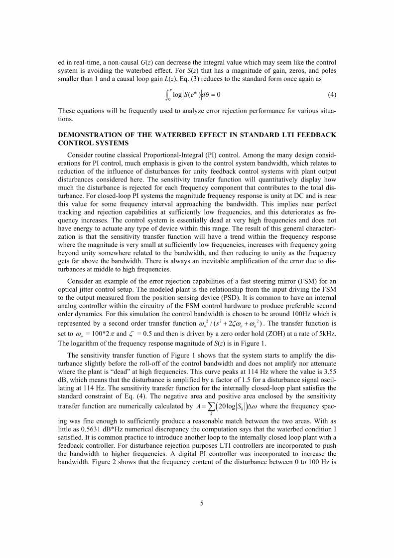
Consider routine classical Proportional-Integral (PI) control. Among the many design consid-erations for PI control, much emphasis is given to the control system bandwidth, which relates to reduction of the influence of disturbances for unity feedback control systems with plant output disturbances considered here. The sensitivity transfer function will quantitatively display how much the disturbance is rejected for each frequency component that contributes to the total dis-turbance. For closed-loop PI systems the magnitude frequency response is unity at DC and is near this value for some frequency interval approaching the bandwidth. This implies near perfect tracking and rejection capabilities at sufficiently low frequencies, and this deteriorates as fre-quency increases. The control system is essentially dead at very high frequencies and does not have energy to actuate any type of device within this range. The result of this general characteri-zation is that the sensitivity transfer function will have a trend within the frequency response where the magnitude is very small at sufficiently low frequencies, increases with frequency going beyond unity somewhere related to the bandwidth, and then reducing to unity as the frequency gets far above the bandwidth. There is always an inevitable amplification of the error due to dis-turbances at middle to high frequencies.

Consider an example of the error rejection capabilities of a fast steering mirror (FSM) for an optical jitter control setup. The modeled plant is the relationship from the input driving the FSM to the output measured from the position sensing device (PSD). It is common to have an internal analog controller within the circuitry of the FSM control hardware to produce preferable second order dynamics. For this simulation the control bandwidth is chosen to be around 100Hz which is represented by a second order transfer function 2 2 2/ ( 2 )n n ns . The transfer function is

set to n = 100*2 and = 0.5 and then is driven by a zero order hold (ZOH) at a rate of 5kHz. The logarithm of the frequency response magnitude of S(z) is in Figure 1.

The sensitivity transfer function of Figure 1 shows that the system starts to amplify the dis-turbance slightly before the roll-off of the control bandwidth and does not amplify nor attenuate where the plant is “dead” at high frequencies. This curve peaks at 114 Hz where the value is 3.55 dB, which means that the disturbance is amplified by a factor of 1.5 for a disturbance signal oscil-lating at 114 Hz. The sensitivity transfer function for the internally closed-loop plant satisfies the standard constraint of Eq. (4). The negative area and positive area enclosed by the sensitivity

transfer function are numerically calculated by 20log kk

A S where the frequency spac-

ing was fine enough to sufficiently produce a reasonable match between the two areas. With as little as 0.5631 dB*Hz numerical discrepancy the computation says that the waterbed condition I satisfied. It is common practice to introduce another loop to the internally closed loop plant with a feedback controller. For disturbance rejection purposes LTI controllers are incorporated to push the bandwidth to higher frequencies. A digital PI controller was incorporated to increase the bandwidth. Figure 2 shows that the frequency content of the disturbance between 0 to 100 Hz is

6

nearly reduced by 80 % by adding the PI controller. However the high frequency range is signifi-cantly amplified due to the waterbed effect. This displays the typical manner in which the water-bed effect operates in feedback control systems.

0 100 200 300 400 500-40

-35

-30

-25

-20

-15

-10

-5

0

5

Frequency (Hz)

20lo

g|S

(ei

)| (d

B)

Sensitivity transfer functionPlant dynamics

AreaDifference:

0.5631 dB*Hz

Negative Area: -710.8333 dB*Hz

Positive Area: 710.2702 dB*Hz

0 100 200 300 400 500 600 700

-25

-20

-15

-10

-5

0

5

10

15

Frequency (Hz)

20lo

g|S

(ei

)| (d

B)

Plant with high bandwidth digital PI controllerOriginal Plant

Negative Area: -2.4725e+03 dB*Hz

Positive Area: 2.4726e+03 dB*Hz

Figure 1. The waterbed effect in classical feed-back systems

Figure 2. Increasing the control bandwidth of the system with classical PI

REPETITIVE CONTROL

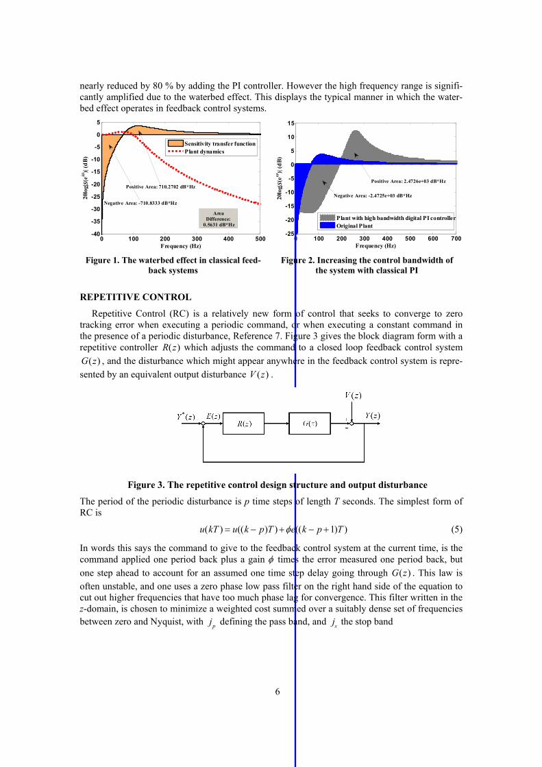
Repetitive Control (RC) is a relatively new form of control that seeks to converge to zero tracking error when executing a periodic command, or when executing a constant command in the presence of a periodic disturbance, Reference 7. Figure 3 gives the block diagram form with a repetitive controller R(z) which adjusts the command to a closed loop feedback control system

G(z) , and the disturbance which might appear anywhere in the feedback control system is repre-

sented by an equivalent output disturbance V (z) .

Figure 3. The repetitive control design structure and output disturbance

The period of the periodic disturbance is p time steps of length T seconds. The simplest form of RC is

u(kT ) u((k p)T )e((k p 1)T ) (5)

In words this says the command to give to the feedback control system at the current time, is the command applied one period back plus a gain times the error measured one period back, but

one step ahead to account for an assumed one time step delay going through G(z) . This law is often unstable, and one uses a zero phase low pass filter on the right hand side of the equation to cut out higher frequencies that have too much phase lag for convergence. This filter written in the z-domain, is chosen to minimize a weighted cost summed over a suitably dense set of frequencies between zero and Nyquist, with

jp

defining the pass band, and js the stop band

7

H (z) a

kzk

kn

n

JH [1 H (e

i jT )]j0

jp

[1 H (ei jT )]* [H (e

i jT )][H (ei jT )]*

j js

N1

(6)

The RC law can be generalized to include a compensator F(z) to adjust phase and amplitude of the error signal, producing the following RC controller transfer function

U (z) H (z)[z pU (z)F(z)z p E(z)] R(z) F(z)H (z)

z p H (z) (7)

Such RC laws are capable of annihilating the DC offset, the fundamental frequency of the ad-dressed period p time steps, and all associated harmonics up to Nyquist frequency, or up to the cutoff frequency. The sensitivity transfer function for the closed-loop RC law is the transfer func-tion from V (z) to error E(z) , or S(z) = 1/(1 + R(z)G(z)). A repetitive control system is stable for all possible periods, if and only if the following inequality is satisfied (Reference 8)

H (z)[1F(z)G(z)] 1 z eiT (8)

UNDESIRABLE WATERBED BEHAVIOR IN SIMPLE RC

Various relatively simple methods of designing repetitive controllers have been developed. One attractive simple design method somewhat analogous to the design of PID controllers is pre-sented in Reference 9. It modifies the simplest RC law, Eq. (5), by introducing a linear phase lead , i.e. the k p 1 is replaced by k p . This allows one to introduce a phase lead in the

error signal used, which can offset phase lag going through the feedback control system G(z) ,

allowing one to have a higher cutoff in H (z) . As in PID control, there are 3 parameters to adjust

when designing the controller, , , and the cutoff frequency. These can be adjusted rather simply in hardware without having a model, and hence one can rather simply improve the per-formance of an existing feedback control system by simple tuning of parameters in hardware.

Consider an example of such a design, where p = 50, G(z) is kept the same as the previous classical control example, H(z) of 51 gains and 1 is used to stabilize the RC law, and F(z) is

the phase lead compensator z . Figure 4 plots the frequency response of |1-F(z)G(z)| with differ-

ent values of , to determine which value makes this go above unity, i.e. which value allows the highest frequency cutoff of the learning process, or which plot first exceeds unity at the highest frequency. Different integer values up to 10 are computed and the value 6 produces the high-est frequency at which the plot exceeds unity. Including such a cutoff, one obtains the corre-sponding sensitivity transfer function magnitude plotted in Figure 5. There are notches going to zero at each addressed frequency up to the cutoff, DC, the fundamental, and harmonics. The notches get narrower with higher harmonics, requiring more accurate knowledge of the frequency to obtain the desired cancellation. The waterbed effect has the property that the frequencies be-tween the addressed frequencies are amplified, and one peak very near the first harmonic fre-quency is amplified by a factor of 12. Slight error in the knowledge of this frequency could result in amplification by a factor of 12 instead of attenuation to zero as intended. We seek methods to avoid such amplification between addressed frequencies, and if possible to push the required am-plification to high frequencies.

8

ATTEMPT TO MODIFY THE CUTOFF FILTER TO SHIFT AMPLIFICATION TO HIGHER FREQUENCIES

We note that the ideal cutoff filter has the property that above the cutoff there is no attenua-tion, and no amplification. One objective is to shift the amplification to these high frequencies, which suggests the use of a modified filter. Reference 10 studied the use of a cutoff filter H (z) tuned to be the least attenuation possible to maintain stability but within a tolerance. This value comes from the minimum attenuation needed to satisfy Eq. (8). Then amplification becomes al-lowed at frequencies above the start of the cutoff. Figure 6 from Reference 10 shows the sensi-tivity transfer function of a system with a perfect zero phase low pass filter cutoff. The amplifica-tion between harmonics at low frequencies is the result of model error. Figure 7 shows the result of using the smallest possible attenuation at each frequency. The plot resembles more the sensi-tivity transfer function plots for a classical feedback control system such as that given above. But there is no resulting benefit in reducing the amplifications between addressed frequencies in the low frequency range. The waterbed effect is behaving more locally, and allows partial notches above the cutoff, in exchange for amplification at higher frequencies further above the cutoff. In some situations this could be helpful, but it does not produce the effect we are searching for.

0 500 1000 1500 2000 25000

0.5

1

1.5

Frequency (Hz)

|1- F

( z) G

( z)|

F(z) = z6

F(z) = z

F(z) = z10

0 500 1000 1500 2000 25000

2

4

6

8

10

12

14

Frequency (Hz)

| S(ei

)|

F(z) = z6, H(z) cutoff @ 800 HzOptimal F(z) with no cutoff H(z)

Large error amplification

Figure 4. |1-F(z)G(z)|, F(z) is a phase lead compensator

Figure 5. Comparing sensitivity transfer functions with F(z) z used to pick 6

as the optimal value

Figure 6. Sensitivity transfer function with perfect cutoff H(z)

Figure 7. Attempt to move low frequency amplification to high frequency by use of a

gentle cutoff

500 600 700 800 900 1000 1100 1200

0.94

0.96

0.98

1

1.02

1.04

1.06

1.08

Frequency (Hz)

|1- F

( z) G

( z)|

F(z) = z6

F(z) = z

F(z) = z10

Cutoff @ 800 Hz

9

IMPROVED WATERBED BY IMPROVED COMPENSATOR DESIGN

The RC law for Figures 4 and 5 is a simple law that can be tuned in hardware without needing a model. Now consider what happens if one uses a model to design the compensator F(z) aiming

to make the left hand side of Eq. (8) zero (with H (z) 1, and 1). This is accomplished by

designing an F(z) to minimize over a suitably dense set of frequencies up to Nyquist as done in

Eq. (6), the square of 1 F(z)G(z) with z eiT , where

1 2 0 ( 1) ( )1 2 1( ) m m n m n m

m n nF z a z a z a z a z a z (9)

J [1G(ei jT )F(ei jT )]j0

N

[1G(ei jT )F(ei jT )]* (10)

One examines various choices for m and n. In other words, we make an approximation of the in-verse of the frequency response of G(z) (see Reference 8). A relatively small number of terms is sufficient to produce a near zero value of this cost function. The resulting sensitivity function is shown by the dotted curve in Figure 5 written for the case G(eiT )F(eiT ) 1 . There is substantial improvement compared to the solid curve in that figure, with the peak values reduced from above 12 down to a maximum amplification of 2, and these peaks appear between all harmonics (this is eliminated above a cutoff if such a filter is needed due to model error at high frequency). One can easily understand this maximum value. For a frequency half way between harmonics, looking back one period of the addressed frequency will result in looking back to a point 180 deg out of phase for the frequency halfway between. The sensitivity transfer function from V (z) to error

E(z) is S(z) (1 z p )V (z) , whose value is 2 at this frequency. Of course, the reduction in the peak value is a substantial improvement achieved at the cost of making and using a model of the system, presumably one that is good to high frequencies. In the list of objectives in the Introduc-tion, item (i) is somewhat addressed, but item (ii) is not addressed, the improved compensator design is unable to push the waterbed amplification to higher frequencies.

THE BENEFITS OF SLOW LEARNING

In the previous section, the fact that the disturbance frequency half way between harmonics has a 180 deg phase shift one period of p time steps back, meant that one added the disturbance to itself in the sensitivity transfer function. If we now slow down the learning, by introducing a gain less than unity in the repetitive control law, then there is less amplification. Computing the

sensitivity transfer function for this case with F(z)G(z) 1 for z eiT , produces

S(z) (z p 1) / (z p (1)) . When the frequency is halfway between harmonics, zp 1 and

this becomes 2 / (2) . Decreasing decreases the height of the peaks. For small , expanding

in a Taylor series, the amplification factor is approximately (1 / 2 ) . Thus, amplification can be made arbitrarily small by having repetitive control updates have an arbitrarily small gain.

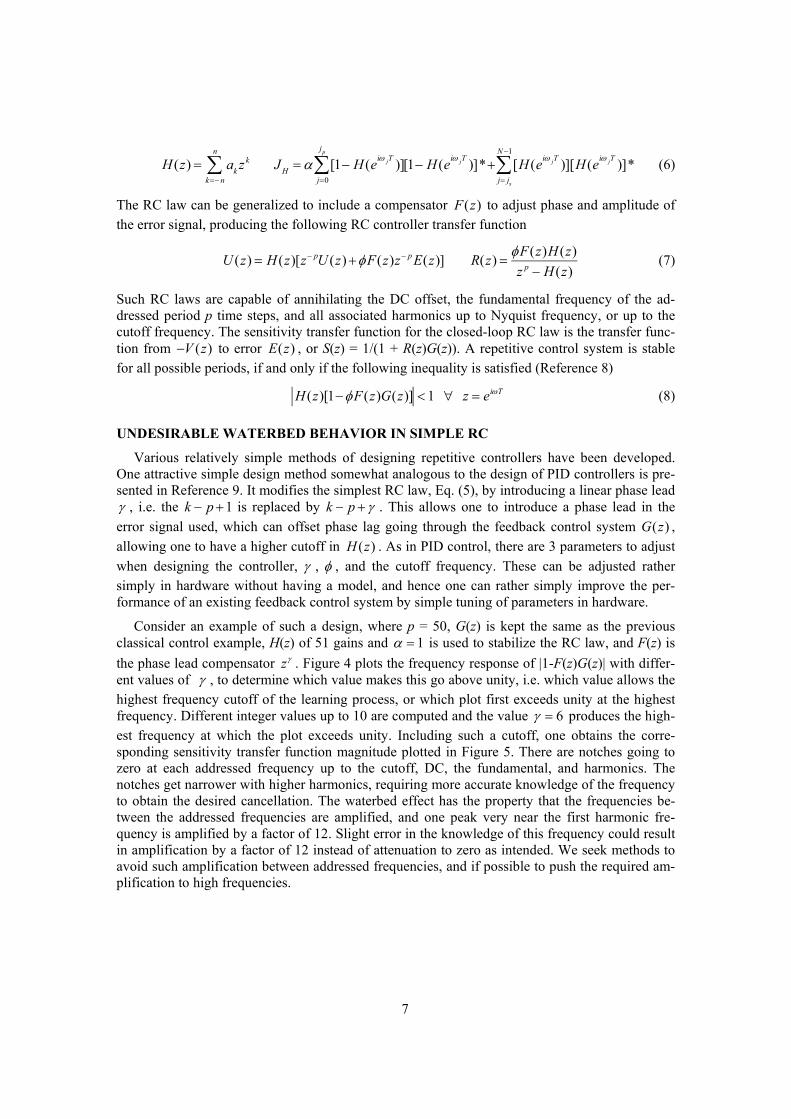
Consider an example where H (z) 1, F(z)G(z) 1 for z eiT , sample rate is again 5kHz,

and the RC is addressing period p 10 so that the fundamental is 500Hz. Figure 8 shows the

magnitude frequency response of the sensitivity transfer function with gain 1, this time the magnitude is shown in dB. Again the amplification is by a factor of 2, which is about 6 dB. Fig-ure 9 zooms in, and compares unity gain to gain 0.1 . We observe that the reduction in the amplification peaks between addressed frequencies is done at the expense of producing narrow

10

notches. Hence, objective (i) is addressed arbitrarily well, at the expense of objective (iii), making the notches at addressed frequencies arbitrarily narrow. Again, we have no way to address objec-tive (ii). According to the waterbed effect, on this dB diagram the area above zero that corre-sponds to amplification must equal the area below zero that produces attenuation of errors. Since the notches actually go to negative infinity, it is not easy to compute the area below zero. Our numerical computation gives areas above and below zero to be equal to within 0.2531. The areas above and below zero have been reduced significantly from 7.0153e+03 to 910.6391, and this is accomplished by making the notches narrower. This approach to preventing significant amplifica-tion, and this is accomplished everywhere in the frequency spectrum, can be used only when one knows the disturbance frequency accurately. Uncertainty in the frequency, numerical roundoff of the period, and fluctuations in the period, limit one’s ability prevent substantial amplification in practice.

0 500 1000 1500 2000 2500-25

-20

-15

-10

-5

0

5

10

Frequency (Hz)

20lo

g|S

(ei

)| (d

B)

Area Difference:0.3000 dB*Hz

Positive Area:7.0153e+03 dB*Hz

Negative Area:-7.0150e+03 dB*Hz

900 1000 1100 1200 1300 1400-25

-20

-15

-10

-5

0

5

Frequency (Hz)

20lo

g|S

(ei

)| (d

B)

RC with = 1RC with = 0.1

AreaDifference:

0.2531 dB*Hz

Negative Area:-910.3859 dB*Hz

Positive Area:910.6391 dB*Hz

Figure 8. The Waterbed effect with unity gain

Figure 9. Comparing the waterbed effect with an RC gain of 1 and 0.1

COMMENTS ON THE ACTUAL ERROR BETWEEN ADDRESSED FREQUENCIES

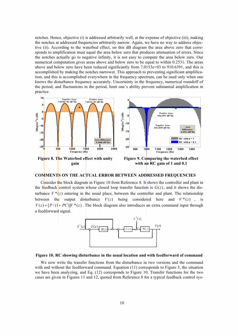
Consider the block diagram in Figure 10 from Reference 8. It shows the controller and plant in the feedback control system whose closed loop transfer function is G(z) , and it shows the dis-

turbance V *(z) entering in the usual place, between the controller and plant. The relationship

between the output disturbance V (z) being considered here and V *(z) , is

V (z) [P / (1 PC)]V *(z) . The block diagram also introduces an extra command input through a feedforward signal.

Figure 10. RC showing disturbance in the usual location and with feedforward of command

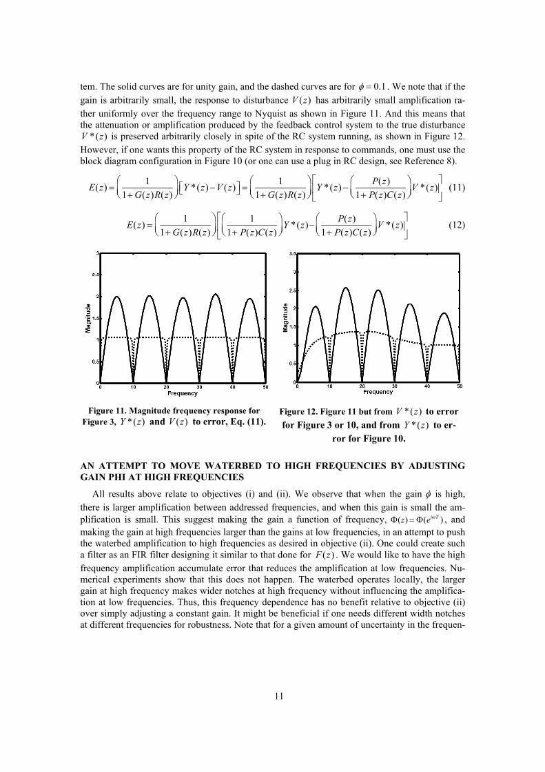
We now write the transfer functions from the disturbance in two versions and the command with and without the feedforward command. Equation (11) corresponds to Figure 3, the situation we have been analyzing, and Eq. (12) corresponds to Figure 10. Transfer functions for the two cases are given in Figures 11 and 12, quoted from Reference 8 for a typical feedback control sys-

11

tem. The solid curves are for unity gain, and the dashed curves are for 0.1 . We note that if the

gain is arbitrarily small, the response to disturbance V (z) has arbitrarily small amplification ra-ther uniformly over the frequency range to Nyquist as shown in Figure 11. And this means that the attenuation or amplification produced by the feedback control system to the true disturbance

V *(z) is preserved arbitrarily closely in spite of the RC system running, as shown in Figure 12. However, if one wants this property of the RC system in response to commands, one must use the block diagram configuration in Figure 10 (or one can use a plug in RC design, see Reference 8).

E(z)

1

1G(z)R(z)

Y *(z)V (z) 1

1G(z)R(z)

Y *(z)P(z)

1 P(z)C(z)

V *(z)

(11)

E(z)

1

1G(z)R(z)

1

1 P(z)C(z)

Y *(z)

P(z)

1 P(z)C(z)

V *(z)

(12)

Figure 11. Magnitude frequency response for Figure 3, Y *(z) and V (z) to error, Eq. (11).

Figure 12. Figure 11 but from V *(z) to error

for Figure 3 or 10, and from Y *(z) to er-ror for Figure 10.

AN ATTEMPT TO MOVE WATERBED TO HIGH FREQUENCIES BY ADJUSTING GAIN PHI AT HIGH FREQUENCIES

All results above relate to objectives (i) and (ii). We observe that when the gain is high, there is larger amplification between addressed frequencies, and when this gain is small the am-plification is small. This suggest making the gain a function of frequency, (z) (eiT ) , and making the gain at high frequencies larger than the gains at low frequencies, in an attempt to push the waterbed amplification to high frequencies as desired in objective (ii). One could create such a filter as an FIR filter designing it similar to that done for F(z) . We would like to have the high frequency amplification accumulate error that reduces the amplification at low frequencies. Nu-merical experiments show that this does not happen. The waterbed operates locally, the larger gain at high frequency makes wider notches at high frequency without influencing the amplifica-tion at low frequencies. Thus, this frequency dependence has no benefit relative to objective (ii) over simply adjusting a constant gain. It might be beneficial if one needs different width notches at different frequencies for robustness. Note that for a given amount of uncertainty in the frequen-

12

cy of the fundamental, the corresponding uncertainty for the first harmonic is larger by a factor of two, etc., so such widening of higher frequency notches might be of practical importance.

DESIGN OF FILTERS TO CREATE LOCAL ADJUSTMENTS OF THE WATERBED EFFECT

Reducing the gain addressed objective (i) to decrease peaks between harmonics, but did so by making narrow notches contrary to the desire of objective (ii). Figure 13 considers gains between 0.01 and 1.99. According to Eq. (8), the latter value is the maximum gain consistent with stability (for H (z) 1 and for a perfect compensator F(eiT )G(eiT ) 1 ), and it produces the widest notches as shown with very large amplification between harmonics. The vertical scale is in dB so the am-plification is more than 2 orders of magnitude. The smaller gain produces very small amplifica-tion, not visible to graphical accuracy. Now we try to decrease the peaks between harmonics by using a large gain for such frequencies, and try to widen the notches at the same time by using a small gain in the neighborhood of the notches. Figure 14 (solid line) plots the chosen desired magnitude response of (eiT ) , which uses a linear transition range on each side of the 1.99 peaks where these curves rapidly descend to meet 0.01.The system considered is the same as in Figures 8 and 9.

600 800 1000 1200 1400

-40

-20

0

20

40

Frequency (Hz)

20lo

g|S

(ei

)| (d

B)

RC gain = 1RC gain = 1.99RC gain = 0.01

0 500 1000 1500 2000 25000

0.5

1

1.5

2

Frequency (Hz)

| ( ei

)|

Desired frequency response for (z)Actual freq. response of (z) with 181 filter gains

Figure 13. The tradeoff of notch width vs. peaks between harmonics for possible sta-

bilizing values of

Figure 14. Magnitude frequency response of chosen zero-phase FIR filter ( )z

The method of producing such a response function develops a zero phase FIR filter. This is optimal considering that according to Eq. (8) zero phase allows the maximum possible range on the magnitude while maintaining stability. A type I linear-phase FIR filter (symmetric impulse response with odd length) of order N is used, having the form

( ) ( )M

k

k M

z k z

(13)

were M is the number of future time steps of ( )k (Reference 11). The total number of filter

weights is N = (M+1)/2, zero phase requires that the symmetry condition ( )k = ( )k is satis-

fied. Zero phase requires that the filter be noncausal having M future time steps of ( )k . This can be used in real time because it operates on data from the previous period, provided that M is not so large compared to p that future data becomes required. In the present situation we do not con-sider the time delay through G(z) and the time steps needed for F(z) , so the maximum M is p.

13

The zero-phase FIR ( )z filter is designed analogously to the design of F(z) as in References 12 and 8, and picks the coefficients in Eq. (13) to minimize

0

[1 ( ) ( )][1 ( ) ( )]i i i iJ e e e e

(7)

where ( )ie is the inverse of the desired frequency response corresponding to the solid line in

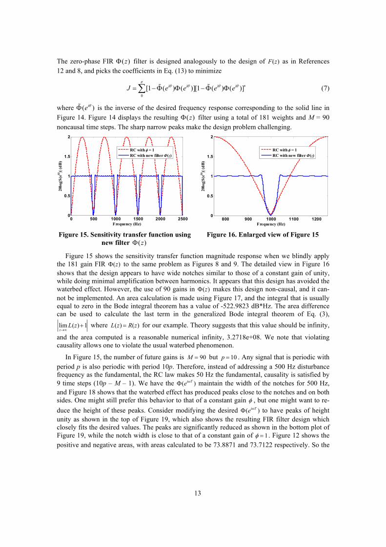
Figure 14. Figure 14 displays the resulting ( )z filter using a total of 181 weights and M = 90 noncausal time steps. The sharp narrow peaks make the design problem challenging.

0 500 1000 1500 2000 25000

0.5

1

1.5

2

Frequency (Hz)

20lo

g|S

(ei

)| (d

B)

RC with = 1RC with new filter (z)

800 900 1000 1100 1200

0

0.5

1

1.5

2

Frequency (Hz)

20lo

g|S

(ei

)| (d

B)

RC with = 1RC with new filter (z)

Figure 15. Sensitivity transfer function using new filter ( )z

Figure 16. Enlarged view of Figure 15

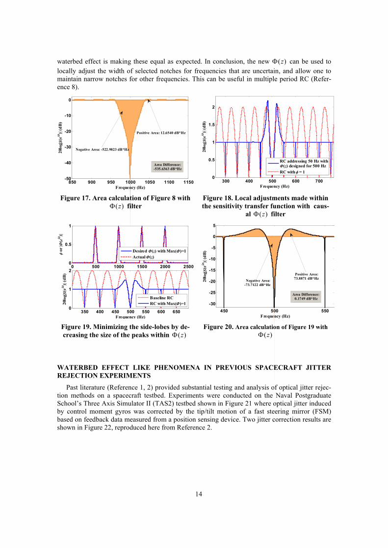
Figure 15 shows the sensitivity transfer function magnitude response when we blindly apply the 181 gain FIR (z) to the same problem as Figures 8 and 9. The detailed view in Figure 16 shows that the design appears to have wide notches similar to those of a constant gain of unity, while doing minimal amplification between harmonics. It appears that this design has avoided the waterbed effect. However, the use of 90 gains in (z) makes this design non-causal, and it can-not be implemented. An area calculation is made using Figure 17, and the integral that is usually equal to zero in the Bode integral theorem has a value of -522.9823 dB*Hz. The area difference can be used to calculate the last term in the generalized Bode integral theorem of Eq. (3),

limz

L(z)1 where L(z) R(z) for our example. Theory suggests that this value should be infinity,

and the area computed is a reasonable numerical infinity, 3.2718e+08. We note that violating causality allows one to violate the usual waterbed phenomenon.

In Figure 15, the number of future gains is M 90 but p 10 . Any signal that is periodic with period p is also periodic with period 10p. Therefore, instead of addressing a 500 Hz disturbance frequency as the fundamental, the RC law makes 50 Hz the fundamental, causality is satisfied by 9 time steps (10p – M – 1). We have the (eiT ) maintain the width of the notches for 500 Hz, and Figure 18 shows that the waterbed effect has produced peaks close to the notches and on both sides. One might still prefer this behavior to that of a constant gain , but one might want to re-

duce the height of these peaks. Consider modifying the desired (eiT ) to have peaks of height unity as shown in the top of Figure 19, which also shows the resulting FIR filter design which closely fits the desired values. The peaks are significantly reduced as shown in the bottom plot of Figure 19, while the notch width is close to that of a constant gain of 1. Figure 12 shows the positive and negative areas, with areas calculated to be 73.8871 and 73.7122 respectively. So the

14

waterbed effect is making these equal as expected. In conclusion, the new ( )z can be used to locally adjust the width of selected notches for frequencies that are uncertain, and allow one to maintain narrow notches for other frequencies. This can be useful in multiple period RC (Refer-ence 8).

850 900 950 1000 1050 1100 1150-50

-40

-30

-20

-10

0

Frequency (Hz)

20lo

g|S

(ei

)| (d

B)

Area Difference:-535.6363 dB*Hz

Positive Area: 12.6540 dB*Hz

Negative Area: -522.9823 dB*Hz

300 400 500 600 7000

0.5

1

1.5

2

Frequency (Hz)

20lo

g|S

(ei

)| (d

B)

RC addressing 50 Hz with (z) designed for 500 Hz

RC with = 1

Figure 17. Area calculation of Figure 8 with ( )z filter

Figure 18. Local adjustments made within the sensitivity transfer function with caus-

al ( )z filter

0 500 1000 1500 2000 25000

0.5

1

or

| ( ei

)|

350 400 450 500 550 600 6500

1

2

Frequency (Hz)

20lo

g|S

(ei

)| (d

B)

Desired (z) with Max( )=1Actual (z)

Baseline RCRC with Max( )=1

450 500 550

-30

-25

-20

-15

-10

-5

0

5

Frequency (Hz)

20lo

g|S

(ei

)| (d

B)

Positive Area:73.8871 dB*Hz

Negative Area:-73.7122 dB*Hz

Area Difference:0.1749 dB*Hz

Figure 19. Minimizing the side-lobes by de-creasing the size of the peaks within ( )z

Figure 20. Area calculation of Figure 19 with ( )z

WATERBED EFFECT LIKE PHENOMENA IN PREVIOUS SPACECRAFT JITTER REJECTION EXPERIMENTS

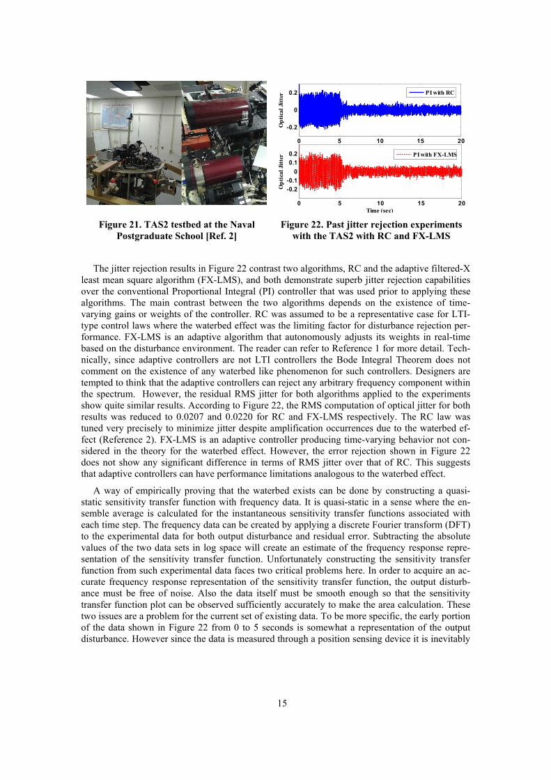
Past literature (Reference 1, 2) provided substantial testing and analysis of optical jitter rejec-tion methods on a spacecraft testbed. Experiments were conducted on the Naval Postgraduate School’s Three Axis Simulator II (TAS2) testbed shown in Figure 21 where optical jitter induced by control moment gyros was corrected by the tip/tilt motion of a fast steering mirror (FSM) based on feedback data measured from a position sensing device. Two jitter correction results are shown in Figure 22, reproduced here from Reference 2.

15

0 5 10 15 20

-0.2

0

0.2

Op

tica

l Jit

ter

0 5 10 15 20

-0.2

-0.1

0

0.1

0.2

Time (sec)

Op

tica

l Jit

ter

PI with RC

PI with FX-LMS

Figure 21. TAS2 testbed at the Naval Postgraduate School [Ref. 2]

Figure 22. Past jitter rejection experiments with the TAS2 with RC and FX-LMS

The jitter rejection results in Figure 22 contrast two algorithms, RC and the adaptive filtered-X least mean square algorithm (FX-LMS), and both demonstrate superb jitter rejection capabilities over the conventional Proportional Integral (PI) controller that was used prior to applying these algorithms. The main contrast between the two algorithms depends on the existence of time-varying gains or weights of the controller. RC was assumed to be a representative case for LTI-type control laws where the waterbed effect was the limiting factor for disturbance rejection per-formance. FX-LMS is an adaptive algorithm that autonomously adjusts its weights in real-time based on the disturbance environment. The reader can refer to Reference 1 for more detail. Tech-nically, since adaptive controllers are not LTI controllers the Bode Integral Theorem does not comment on the existence of any waterbed like phenomenon for such controllers. Designers are tempted to think that the adaptive controllers can reject any arbitrary frequency component within the spectrum. However, the residual RMS jitter for both algorithms applied to the experiments show quite similar results. According to Figure 22, the RMS computation of optical jitter for both results was reduced to 0.0207 and 0.0220 for RC and FX-LMS respectively. The RC law was tuned very precisely to minimize jitter despite amplification occurrences due to the waterbed ef-fect (Reference 2). FX-LMS is an adaptive controller producing time-varying behavior not con-sidered in the theory for the waterbed effect. However, the error rejection shown in Figure 22 does not show any significant difference in terms of RMS jitter over that of RC. This suggests that adaptive controllers can have performance limitations analogous to the waterbed effect.

A way of empirically proving that the waterbed exists can be done by constructing a quasi-static sensitivity transfer function with frequency data. It is quasi-static in a sense where the en-semble average is calculated for the instantaneous sensitivity transfer functions associated with each time step. The frequency data can be created by applying a discrete Fourier transform (DFT) to the experimental data for both output disturbance and residual error. Subtracting the absolute values of the two data sets in log space will create an estimate of the frequency response repre-sentation of the sensitivity transfer function. Unfortunately constructing the sensitivity transfer function from such experimental data faces two critical problems here. In order to acquire an ac-curate frequency response representation of the sensitivity transfer function, the output disturb-ance must be free of noise. Also the data itself must be smooth enough so that the sensitivity transfer function plot can be observed sufficiently accurately to make the area calculation. These two issues are a problem for the current set of existing data. To be more specific, the early portion of the data shown in Figure 22 from 0 to 5 seconds is somewhat a representation of the output disturbance. However since the data is measured through a position sensing device it is inevitably

16

corrupted by measurement noise, and therefore has a significant amount of ambiguity in acquiring the true output disturbance. Although it is not shown within this paper, numerous attempts were made to filter out the noise of the output disturbance, but this tended to deteriorate the data by eliminating needed information. As a result, the next section considers simulated data and analy-sis.

POSSIBLE WATERBED EFFECT IN ADAPTIVE CONTROL ALGORITHMS

Adaptive control algorithms are nonlinear, and the Bode Integral Theorem says nothing about nonlinear systems. However, for a disturbance environment with stationary statistics, the adapta-tion will eventually converge and the weights of the adaptive controller will become constant making the converged adaptive controller linear. This suggests that the waterbed phenomenon should apply to a fully converged adaptive control system. However, in practice the weights that are adapted in the adaptive control algorithm seem to be subject to random fluctuations even after one considers the system to have converged. If the weights are fluctuating in time, again it is not an LTI system and the waterbed result does not apply to such systems. We now numerically ex-amine how a fully converged adaptive controller with weights that randomly fluctuate about some value exhibit waterbed like behavior.

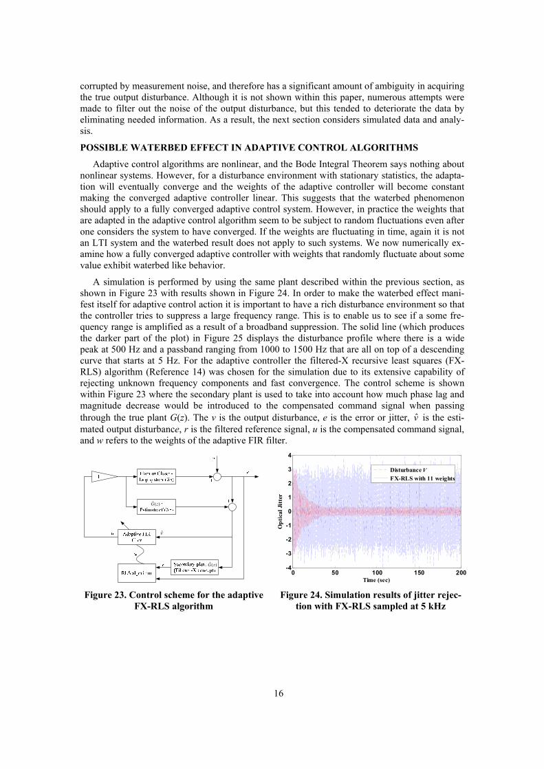
A simulation is performed by using the same plant described within the previous section, as shown in Figure 23 with results shown in Figure 24. In order to make the waterbed effect mani-fest itself for adaptive control action it is important to have a rich disturbance environment so that the controller tries to suppress a large frequency range. This is to enable us to see if a some fre-quency range is amplified as a result of a broadband suppression. The solid line (which produces the darker part of the plot) in Figure 25 displays the disturbance profile where there is a wide peak at 500 Hz and a passband ranging from 1000 to 1500 Hz that are all on top of a descending curve that starts at 5 Hz. For the adaptive controller the filtered-X recursive least squares (FX-RLS) algorithm (Reference 14) was chosen for the simulation due to its extensive capability of rejecting unknown frequency components and fast convergence. The control scheme is shown within Figure 23 where the secondary plant is used to take into account how much phase lag and magnitude decrease would be introduced to the compensated command signal when passing through the true plant G(z). The v is the output disturbance, e is the error or jitter, v̂ is the esti-mated output disturbance, r is the filtered reference signal, u is the compensated command signal, and w refers to the weights of the adaptive FIR filter.

ˆ ( )G z

ˆ ( )G z

v̂

0 50 100 150 200

-4

-3

-2

-1

0

1

2

3

4

Time (sec)

Op

tica

l Jit

ter

Disturbance VFX-RLS with 11 weights

Figure 23. Control scheme for the adaptive FX-RLS algorithm

Figure 24. Simulation results of jitter rejec-tion with FX-RLS sampled at 5 kHz

17

The disturbance rejection simulation results are shown in Figure 24 where the FIR filter had 11 weights, used a forgetting factor of 0.9999, and had an initial inverse covariance matrix of 0.05 times the identity matrix with a dimension of [11 x 11]. One can see in Figure 24 that the error rejection is quite significant and the controller converges near 50 seconds.

0 500 1000 1500 2000 2500-160

-140

-120

-100

-80

-60

-40

-20

0

Frequency (Hz)

Pow

er S

pect

ral D

ensi

ty:

Pow

er/F

req.

(dB

/Hz)

PSD of Disturbance vPSD of e after FX-RLS

Amplification @high frequencies

Attenuated error

0 50 100 150 200

-6000

-4000

-2000

0

2000

4000

6000

Time (sec)

Wei

ghts

of

FX

-RL

S F

IR fi

lter

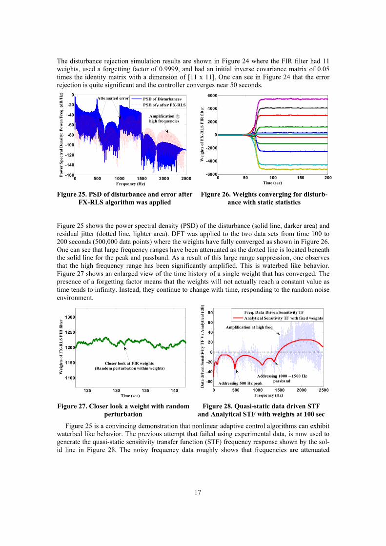
Figure 25. PSD of disturbance and error after FX-RLS algorithm was applied

Figure 26. Weights converging for disturb-ance with static statistics

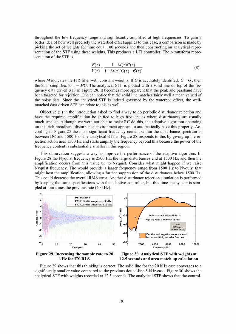
Figure 25 shows the power spectral density (PSD) of the disturbance (solid line, darker area) and residual jitter (dotted line, lighter area). DFT was applied to the two data sets from time 100 to 200 seconds (500,000 data points) where the weights have fully converged as shown in Figure 26. One can see that large frequency ranges have been attenuated as the dotted line is located beneath the solid line for the peak and passband. As a result of this large range suppression, one observes that the high frequency range has been significantly amplified. This is waterbed like behavior. Figure 27 shows an enlarged view of the time history of a single weight that has converged. The presence of a forgetting factor means that the weights will not actually reach a constant value as time tends to infinity. Instead, they continue to change with time, responding to the random noise environment.

125 130 135 140

1100

1150

1200

1250

1300

Time (sec)

Wei

ghts

of

FX

-RL

S F

IR f

ilte

r

Closer look at FIR weights(Random perturbation within weights)

0 500 1000 1500 2000 2500

-60

-40

-20

0

20

40

60

80

Frequency (Hz)

Dat

a d

rive

n S

ensi

tivi

ty T

F V

s A

naly

tica

l (dB

)

Freq. Data Driven Sensitivity TFAnalytical Sensitivity TF with fixed weights

Amplification at high freq.

Addressing 1000 ~ 1500 Hzpassband

Addressing 500 Hz peak

Figure 27. Closer look a weight with random perturbation

Figure 28. Quasi-static data driven STF and Analytical STF with weights at 100 sec

Figure 25 is a convincing demonstration that nonlinear adaptive control algorithms can exhibit waterbed like behavior. The previous attempt that failed using experimental data, is now used to generate the quasi-static sensitivity transfer function (STF) frequency response shown by the sol-id line in Figure 28. The noisy frequency data roughly shows that frequencies are attenuated

18

throughout the low frequency range and significantly amplified at high frequencies. To gain a better idea of how well precisely the waterbed effect applies to this case, a comparison is made by picking the set of weights for time equal 100 seconds and then constructing an analytical repre-sentation of the STF using these weights. This produces a LTI controller. The z-transform repre-sentation of the STF is

E(z)

V (z)

1 M (z)G(z)

1 M (z)[G(z) öG(z)] (8)

where M indicates the FIR filter with constant weights. If G is accurately identified, ˆG G , then the STF simplifies to 1 – MG. The analytical STF is plotted with a solid line on top of the fre-quency data driven STF in Figure 28. It becomes more apparent that the peak and passband have been targeted for rejection. One can notice that the solid line matches fairly well a mean valued of the noisy data. Since the analytical STF is indeed governed by the waterbed effect, the well-matched data driven STF can relate to this as well.

Objective (ii) in the introduction asked to find a way to do periodic disturbance rejection and have the required amplification be shifted to high frequencies where disturbances are usually much smaller. Although we were not able to make RC do this, the adaptive algorithm operating on this rich broadband disturbance environment appears to automatically have this property. Ac-cording to Figure 25 the most significant frequency content within the disturbance spectrum is between DC and 1500 Hz. The analytical STF in Figure 28 responds to this by giving up the re-jection action near 1500 Hz and starts amplify the frequency beyond this because the power of the frequency content is substantially smaller in this region.

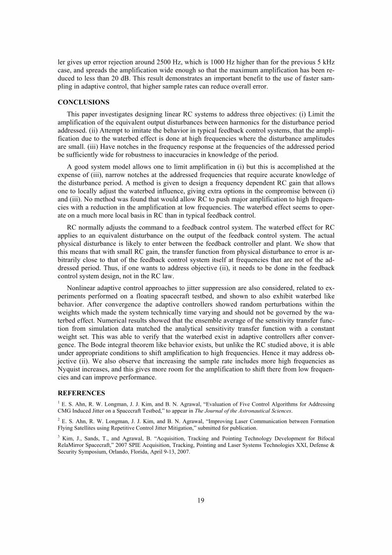
This observation suggests a way to improve the performance of the adaptive algorithm. In Figure 28 the Nyquist frequency is 2500 Hz, the large disturbances end at 1500 Hz, and then the amplification occurs from this value up to Nyquist. Consider what might happen if we raise Nyquist frequency. The would provide a larger frequency range from 1500 Hz to Nyquist that might host the amplification, allowing a further suppression of the disturbances below 1500 Hz. This could decrease the overall RMS error. Another disturbance rejection simulation is performed by keeping the same specifications with the adaptive controller, but this time the system is sam-pled at four times the previous rate (20 kHz).

0 10 20 30 40 50-4

-3

-2

-1

0

1

2

3

4

Time (sec)

Op

tica

l Jit

ter

Disturbance VFX-RLS with sample rate 5 kHzFX-RLS with sample rate 20 kHz

0 2000 4000 6000 8000 10000-80

-60

-40

-20

0

20

Frequency (Hz)

20lo

g|S

(ei

)| (d

B)

Positive and negative areas enclosedby the sensitivity transfer function

Positive Area: 8.8699e+04 dB*Hz

Negative Area: -8.8699e+04 dB*Hz

AreaDifference:

-0.0429 dB*Hz

Figure 29. Increasing the sample rate to 20 kHz for FX-RLS

Figure 30. Analytical STF with weights at 12.5 seconds and area match up calculation

Figure 29 shows that this thinking is correct. The solid line for the 20 kHz case converges to a significantly smaller value compared to the previous dotted-line 5 kHz case. Figure 30 shows the analytical STF with weights recorded at 12.5 seconds. The analytical STF shows that the control-

19

ler gives up error rejection around 2500 Hz, which is 1000 Hz higher than for the previous 5 kHz case, and spreads the amplification wide enough so that the maximum amplification has been re-duced to less than 20 dB. This result demonstrates an important benefit to the use of faster sam-pling in adaptive control, that higher sample rates can reduce overall error.

CONCLUSIONS

This paper investigates designing linear RC systems to address three objectives: (i) Limit the amplification of the equivalent output disturbances between harmonics for the disturbance period addressed. (ii) Attempt to imitate the behavior in typical feedback control systems, that the ampli-fication due to the waterbed effect is done at high frequencies where the disturbance amplitudes are small. (iii) Have notches in the frequency response at the frequencies of the addressed period be sufficiently wide for robustness to inaccuracies in knowledge of the period.

A good system model allows one to limit amplification in (i) but this is accomplished at the expense of (iii), narrow notches at the addressed frequencies that require accurate knowledge of the disturbance period. A method is given to design a frequency dependent RC gain that allows one to locally adjust the waterbed influence, giving extra options in the compromise between (i) and (iii). No method was found that would allow RC to push major amplification to high frequen-cies with a reduction in the amplification at low frequencies. The waterbed effect seems to oper-ate on a much more local basis in RC than in typical feedback control.

RC normally adjusts the command to a feedback control system. The waterbed effect for RC applies to an equivalent disturbance on the output of the feedback control system. The actual physical disturbance is likely to enter between the feedback controller and plant. We show that this means that with small RC gain, the transfer function from physical disturbance to error is ar-bitrarily close to that of the feedback control system itself at frequencies that are not of the ad-dressed period. Thus, if one wants to address objective (ii), it needs to be done in the feedback control system design, not in the RC law.

Nonlinear adaptive control approaches to jitter suppression are also considered, related to ex-periments performed on a floating spacecraft testbed, and shown to also exhibit waterbed like behavior. After convergence the adaptive controllers showed random perturbations within the weights which made the system technically time varying and should not be governed by the wa-terbed effect. Numerical results showed that the ensemble average of the sensitivity transfer func-tion from simulation data matched the analytical sensitivity transfer function with a constant weight set. This was able to verify that the waterbed exist in adaptive controllers after conver-gence. The Bode integral theorem like behavior exists, but unlike the RC studied above, it is able under appropriate conditions to shift amplification to high frequencies. Hence it may address ob-jective (ii). We also observe that increasing the sample rate includes more high frequencies as Nyquist increases, and this gives more room for the amplification to shift there from low frequen-cies and can improve performance.

REFERENCES 1 E. S. Ahn, R. W. Longman, J. J. Kim, and B. N. Agrawal, “Evaluation of Five Control Algorithms for Addressing CMG Induced Jitter on a Spacecraft Testbed,” to appear in The Journal of the Astronautical Sciences. 2 E. S. Ahn, R. W. Longman, J. J. Kim, and B. N. Agrawal, “Improving Laser Communication between Formation Flying Satellites using Repetitive Control Jitter Mitigation,” submitted for publication. 3 Kim, J., Sands, T., and Agrawal, B. “Acquisition, Tracking and Pointing Technology Development for Bifocal RelaMirror Spacecraft,” 2007 SPIE Acquisition, Tracking, Pointing and Laser Systems Technologies XXI, Defense & Security Symposium, Orlando, Florida, April 9-13, 2007.

20

4 M. S. Seron, J. H. Braslavsky, and G. C. Goodwin, Fundamental Limitations in Filtering and Control, Springer Verlag, 1997. 5 T. Songchon and R. W. Longman, “On the Waterbed Effects and Repetitive Control using Zero-Phase Filtering,” Proceedings of the AIAA/AAS Astrodynamics Conference, Santa Barbara, CA, February 2001, AAS 01-196. 6 R. W. Longman, R. Akogyeram, A. Hutton, and J.-N. Juang, “Trade-Offs Between Feedback, Feedforward, and Re-petitive Control for Systems Subject to Periodic Disturbances,” Advances in the Astronautical Sciences, Vol. 108, 2002, pp. 1281-1300 7 T. Yamaguchi, M. Hirata, C. K. Pang, Advances in High-Performance Motion Control of Mechatronic Systems, CRC Press, 2013 8 R. W. Longman, “On the Theory and Design of Linear Repetitive Control Systems.” European Journal of Control, Special Section on Iterative Learning Control, Guest Editor Hyo-Sung Ahn. Vol. 16, No. 5, 2010, pp. 447-496. 9 R. W. Longman, “Iterative Learning Control and Repetitive Control for Engineering Practice,” International Journal of Control, Special Issue on Iterative Learning Control, Vol. 73, No. 10, July 2000, pp. 930-954. 10 Y. Shi and R. W. Longman, “The Influence on Stability Robustness of Compromising on the Zero Tracking Error Requirement in Repetitive Control.” Advances in the Astronautical Sciences, Vol. 139, 2011, pp. 465-483. 11 E. C. Ifeachor and B. W. Jervis, Digital Signal Processing: A Practical Approach, 2nd ed. Pearson Education Lim-ited, 2002. 12 B. Panomruttanarug and R. W. Longman, “Frequency Based Optimal Design of FIR Zero-Phase Filters and Com-pensators for Robust Repetitive Control,” Advances in the Astronautical Sciences, Vol.123, 2006, pp. 219-238. 13 M. Nagashima and R. W. Longman, “Stability and Performance Analysis of Matched Basis Function Repetitive Con-trol in the Frequency Domain.” Advances in the Astronautical Sciences. Vol. 119, 2005, pp. 1581-1600. 14 S.M. Kuo and D.R. Morgan, Active Noise Control Systems: Algorithms and DSP Implementations, Wiley-Interscience, 1996.