i t l s - university of...

I T L S

WORKING PAPER

ITLS-WP-10-05

Willingness to pay for travel time reliability in passenger transport: A review and some new empirical evidence By Zheng Li, David A Hensher and John Rose March 2010 ISSN 1832-570X

INSTITUTE of TRANSPORT and LOGISTICS STUDIES The Australian Key Centre in Transport and Logistics Management

The University of Sydney Established under the Australian Research Council’s Key Centre Program.

NUMBER: Working Paper ITLS-WP-10-05

TITLE: Willingness to pay for travel time reliability in passenger transport: A review and some new empirical evidence

ABSTRACT: This paper reviews and critiques the modelling frameworks and empirical measurement paradigms used to obtain willingness to pay (WTP) for improved travel time reliability, suggesting new directions for ongoing research. We also estimate models to derive values of reliability, scheduling costs and reliability ratios in the context of Australian toll roads and use the new evidence to highlight the important influence of the way that trip time variability is included in stated preference studies in deriving WTP estimates of reliability in absolute terms, and relative to the value of travel time savings.

KEY WORDS: Travel time reliability, passenger transport, value of travel time savings, value of reliability, schedule delay

AUTHORS: Zheng Li, David A Hensher & John M Rose

CONTACT: Institute of Transport and Logistics Studies (C37) The Australian Key Centre in Transport Management The University of Sydney NSW 2006 Australia Telephone: +61 9351 0071 Facsimile: +61 9351 0088 E-mail: [email protected] Internet: http://www.itls.sydney.edu.au

DATE: March 2010

Acknowledgment.

The comments of Wayne Talley and Ken Small are appreciated

.

mailto:[email protected]

http://www.itls.usyd.edu.au/

Willingness to pay for travel time reliability in passenger transport: A review and some new empirical evidence

Li, Hensher & Rose

1. Introduction

It is increasingly recognised that travel time reliability, and its valuation, is important to travellers, and hence should be given greater emphasis in transport policy and performance management, and hence must be included in patronage forecasting and appraisal studies. For example, in the Netherlands, improving travel time reliability is regarded as a primary objective for the Ministry of Transport, Public Works and Water Management in the coming decade (AVV 2004). The UK government aims to achieve a 25 percent reduction in train delays of over 30 minutes, and improve the reliability of train service from 88 percent in 2007 to 92.6 percent by 2014 (Department for Transport 2007). In the USA, the value of travel time reliability has important implications on road pricing to ensure more efficient use of toll roads (see e.g., Small et al. 2005; Brownstone and Small 2005).

Reliability always implies a notion of repetition. Hence, travel time reliability studies measure the variability in travel times over repeated journeys. Travel time variability is a feature of transport systems, which adds additional costs and uncertainty to travellers. Travel time variability may impact a variety of travel choices (e.g., time, route and mode), however an adjustment to departure time typically represents the easiest response to expected or experienced travel time variability. Gaver (1968) represents one of the earliest studies to investigate individuals’ behavioural responses to travel time variability, by including it within a framework based on utility maximisation. Graver found that a traveller would plan an earlier departure time when facing travel time variability, compared with the circumstances given known certain travel times. Knight (1974) proposed a “safety margin” hypothesis to explain a similar response of travellers to travel time variability. Guttman (1979) and Mensashe and Guttman (1986) suggested that risk-averse travellers would choose the transport mode with less travel time variability. Recently, empirical studies have revealed that travellers are willing to pay for the reduction in travel time variability in addition to travel time savings (see e.g., Senna 1994; Small et al., 1999; Hensher 2001a,b; Bhat and Sardesai 2006), and some studies even estimated higher values for reducing travel variability than for reducing the scheduled journey time or the average travel time (see e.g., Asensio and Matas 2008; Batley and Ibáñez 2009).

An early review on travel time reliability by Noland and Polak (2002) discussed some theoretical and empirical issues related to behavioural responses to reliability of time, such as behavioural responses associated with departure time choice in scheduling models with or without fixed service intervals, some stated preference (SP) data collection issues, the impact of modal attributes on parameter estimates, etc. However, all reviewed studies in Noland and Polak (2002) were published before 2001. Since 2000, there have been substantial developments in this area of research, using mixtures of SP and revealed preference (RP) data. We include RP studies (see e.g., Lam and Small 2001) and combined RP and SP studies (see e.g., Small et al. 2005) in our review. Further, Noland and Polak (2002) focused on only one modelling framework, that being the scheduling model.

In this paper, we examine other frameworks such as the mean-variance model and the mean lateness model (a newly developed model). In comparison to Noland and Polak (2002), we take a closer look at the variety of SP experiments that have been investigated (e.g., clock-face format, vertical bars) and compare their relative performance.

Tseng (2008) undertook a meta analysis (unpublished) of the valuation of travel time reliability and found that the specification of the utility function is the only statistically significant factor to systematically influence the ratio of the value of reliability (VOR) to the value of travel time savings (VTTS). However, Tseng’s meta regression model did not consider the experiment design as a potential source, in particular the way of presenting of travel time variability, which has been argued by many analysts to be a critical influence on the valuation of travel time reliability (see e.g., Hollander 2006, Batley and Ibáñez 2009). In this paper, we take a closer look at the impact of different presentations of SP experiments on estimates of willingness to pay (WTP) for improved reliability. We also draw together the implications of the WTP estimates on transport planning methods.

The organisation of the paper is as follows. First, we introduce the characteristics of travel time variability. This is followed by the presentation of three types of models to estimate the impact of

1

Willingness to pay for travel time reliability in passenger transport: A review and some new empirical evidence Li, Hensher & Rose travel time reliability, and hence value it, namely the mean-variance model, the scheduling model and the mean lateness model. Then, we present different experiments for representing and valuing travel time reliability, and discuss some recent studies, predominantly from the US and the UK. This is followed by empirical analysis of travel time reliability in the context of toll roads in Australia. We then provide some conclusions, together with suggestions for future research.

2. Characteristics of travel time variability

Bates et al. (1987) classified travel time variability into three categories: i) inter-day variability caused by seasonal and day-to-day variations (such as demand fluctuations, accidents, road construction and weather changes), ii) inter-period variability which reflects the impact of differences in departure times and the caused changes in congestion, and iii) inter-vehicle variability mainly due to individual driving styles and traffic signals. Noland and Polak (2002) use similar categories to represent travel time variability; differences in travel time from day-to-day, over the course of the day and even from vehicle to vehicle. Bates et al. (2001) further added that on the demand side, after considering seasonal effects, day-of-week effects and other systematic variations, the residual day-to-day variations are essentially random, whilst the randomness on the supply side is mainly due to incidents (e.g., vehicle breakdowns, signal failures, etc.).

The majority of travel time variability studies have investigated day-to-day variations in travel time, and have explicitly defined travel time reliability as the random variation in travel time (see e.g., Bates et al. 2001; Hollander 2006; Hollander and Steer Davies Gleave 2009), so as to emphasise the stochastic feature of travel time variability. Based on the approach of Noland and Small (1995) in which travel time was divided into the free flow time and congested time, Bates et al. (2001) added an additional component of time, namely travel time variability, which represents the randomness in travel times over repeated trips. The concept of variability suggests that individuals have to make their travel decisions under uncertain circumstances with respect to the travel time; hence they are not able to predict the exact travel time or arrival time before starting their trips, given a departure time. Noland and Polak (2002) emphasised that the distinction between travel time variability and congestion is linked in that travellers have difficulty in predicting the former (e.g., congestion caused by unforeseen road accidents or service cancellations) from day-to-day, while they can to some extent predict the variation in travel time due to congestion (e.g., peak hours vs. off-peak hours). A transport system with severe congestion may have stable day-to-day travel times; hence travellers can capture the systematic variation based on their past experience, so as to anticipate their arrival time. Many measures of travel time variability have been developed in the extant literature; however one common feature is the recognition that travel time distribution is impacted by day-to-day fluctuations on the demand side as well as the supply side of traffic, as shown in Figure 1(van Lint et al. 2008).

2


Li, Hensher & Rose

Figure 1: Factors impacting the distribution of travel time

Travel time variability is indeed random and unpredictable, with the lognormal distribution being the most commonly used distribution to represent it (see e.g., Rietveld et al. 2001; Giuliano 1989), however Bates et al. (2001) found that a generalised Poisson distribution to better describe the delay distribution for train travel time. In the face of travel time variability, travel decisions are made under uncertainty or risk (i.e., probabilities related to alternative travel times); hence a traveller will choose the option that maximises expected utility. Most recent travel time variability studies have embraced this concept in their empirical analyses (see e.g., Small et al. 1999; Bates et al. 2001; Batley and Ibáñez 2009). However, early studies assumed that travellers are utility maximisers within a paradigm that assumes that travel decisions are made under certainty (see e.g., Jackson and Jucker 1982; Small 1982).

3. Theoretical frameworks

3.1 The mean-variance model

Many of the earlier travel time variability studies assumed that variability was the source of disutility, similar to the mean travel time (Jackson and Jucker 1982; Pells, 1987; Black and Towriss, 1993), and that time variability can be represented by the variance or standard deviation1 of travel time (i.e., the mean-variance approach). Jackson and Jucker (1982) proposed a mean-variance framework in which utility, U, is defined as a function of usual (or mean) travel time and the variance, assuming that travellers trade off time against variability (variance), and the objective is to minimise their sum (equation 1).

1 Some SP studies also use the coefficient of variation (i.e., standard deviation divided by mean travel time) in utility function (see e.g., Noland et al. 1998).

3

Willingness to pay for travel time reliability in passenger transport: A review and some new empirical evidence Li, Hensher & Rose

_

( )U T V Tλ= + (1)

where λ is a parameter measuring the influence of variance in travel times; is the usual or mean travel time; and is the variance of travel time.

_

T( )V T

Based on Jackson and Jucker’s two-parameter model (mean travel time and variance), Senna (1994) incorporated the expected utility, E(U) (i.e., the probability weighted average of the utility of the outcomes), approach of Polak (1987) to analyse commuters and non-commuters responses to travel time variability. Senna’s model has three attributes: the expected travel time, standard deviation and cost. Small et al. (1999)2 also estimated values of reliability using the mean-variance model (equation 2).

E( ) ( ) ( )T SDU E T SD T CCβ β β= + + (2)

where Tβ , SDβ and Cβ are the estimated parameters for the expected travel time ( ), the standard deviation of travel time ( ) and travel cost (C) respectively.

( )E T( )SD T

Small et al. (1999) also included some socio-demographic characteristics and trip purposes to capture heterogeneity in VOR, for example, higher values for a commuter trip compared with a non-commuter trip. Similar to the VTTS, the VOR is defined as the ratio of the respective parameters ( SDβ / Cβ ), which measures travellers’ WTP for a unit reduction in variability (shown as the standard deviation) in travel time. Other authors have also estimated mean-variance models (see e.g., Black and Towriss 1993; Abdel-Aty et al. 1995). An important outcome from these studies is the reliability ratio, defined as the marginal rate of substitution between average travel time and travel time variability (i.e., SD / Tβ β ). The estimated reliability ratios vary across studies, with some as high as 2.1 (Batley and Ibáñez 2009) and others as low as 0.1 (Hollander 2006). De Jong et al. (2009) suggested that the agreed ratio for car travel is 0.8 and 1.4 for public transport. Bates et al. (2001) suggest that the ratio should be around 1.3 for car travel and no more than 2.0 for public transport.

3.2 The scheduling model

The scheduling model is an alternative approach to modelling travel time reliability, which takes into account the consequences of unreliable travel time. Unlike the mean-variance model which assumes that travel time variability leads to the loss of utility by itself, the scheduling model considers that disutility is incurred when not arriving at the preferred arrival time (PAT), either early or late. Small (1982) defines the difference between the PAT and the actual arrival time as schedule delay (SD), which Bates et al. (2001) describe as the variations to the preferred arrival time.

( )( )h hSD PAT t T t= − +

(3)

The total travel time ( ) is determined by the departure time ( ). A late arrival (schedule delay late or SDL) relative to the PAT will occur if ; otherwise, it will be a schedule delay early (SDE).

( )htT ht0>hh t(t T( )) PAT+ −

2 The scheduling model is also used in Small et al. (1999).

4


Li, Hensher & Rose

Figure 2: The concept of schedule delay

Small (1982) proposed the scheduling model as a way to understand travellers’ departure time choices in order to satisfy on-time arrival, as given in equation (4).

LU T SDE SDL Dα β γ θ= + + + (4)

T is travel time, SDE is schedule delay early, SDL is schedule delay late, is a dummy variable equal to 1 when there is a SDL and 0 otherwise; and the estimated parameters (

LD, , ,and α β γ θ ) are

assumed to be negative.

The model developed by Small (1982) is for choice under certainty. Noland and Small (1995) advanced Small’s scheduling model to analyse choice under uncertainty by adding in the probability distribution of travel time. The theory underlying Noland and Small’s model is Maximum Expected Utility (MEU) (i.e., to choose the option with the highest value of expected utility). Given travel time variability, travel time (T) is uncertain with a distribution dependent on the departure time ( ) (Bates et al. 2001). Hence, the expected utility of the scheduling model can be expressed as the equation (5), where the possible delay or advance with respect to the preferred arrival time are modelled separately, and their consequences are measured by the estimated parameters

ht

3.

[ ( )] [ ( )] [ ( )] [ ( )] ( )h h h hE U t E T t E SDE t E SDL t P tα L hβ γ θ= + + + (5)

The expected utility ( ) is a function of the expected trave time ( ), the expected schedule delay early ( ), the expected schedule delay late ( ) and the probability of experiencing a late arrival ( ). Bates et al. (2001) suggested that the scheduling method is perfectly suitable for valuing travel time reliability in the passenger car context, given the continuous adjustment of a car driver’s departure time. For public transport users, their ability to adjust departure times is limited by the existence of a timetable offering discrete time choices for departure. Hence, the disutility is more directly linked with variability per se (e.g., standard deviation), compared to that associated with schedule delay. However, Hollander (2006) empirically estimated two models in the context of bus transport, and claimed that, in addition to the mean travel time, variability is better captured in the scheduling model, since disutility caused by the late arrival is significantly higher than that caused by the early arrival.

( )hU t[E S

[ ( )]hE T t[E SDL( hDE t )] )]

( ht( )L hP t

Apart from its application in analysing departure time choice (see e.g., Noland and Small 1995; Hollander 2006), the scheduling model is often applied in other areas of choice analysis, where each alternative offers different levels of travel time variability, departure times, travel times and costs. For example, Asensio and Matas (2008) analysed commuting car drivers’ route choices in Spain. Noland (1999) applied the scheduling model in the context of route choice.

The scheduling model and the mean-variance models are two common approaches to empirical measures of responses to changes in travel time reliability. According to Bates et al. (2001), a mean–

3 The travel time destination needs to be assumed for estimating the values of parameters, which is often assumed to be equi-probable for analysis (see e.g., Small et al. 1999; Bates et al. 2001).

5

Willingness to pay for travel time reliability in passenger transport: A review and some new empirical evidence Li, Hensher & Rose variance model can approximate a scheduling model, under some specific assumptions including: i) that the parameters that define the travel time variability distribution are not time dependent; ii) regular congestion is independent of departure time; iii) there is no lateness penalty and iv) the departure time is continuous. Hollander (2006) applied both types in the context of bus transport for understanding factors influencing passengers’ responses and attitudes to travel time variability with regard to their departure time choice considerations. Small et al. (1999) concluded that “in models with a fully specified set of scheduling costs, it is unnecessary to add an additional cost for unreliability”.

3.3 The mean lateness model

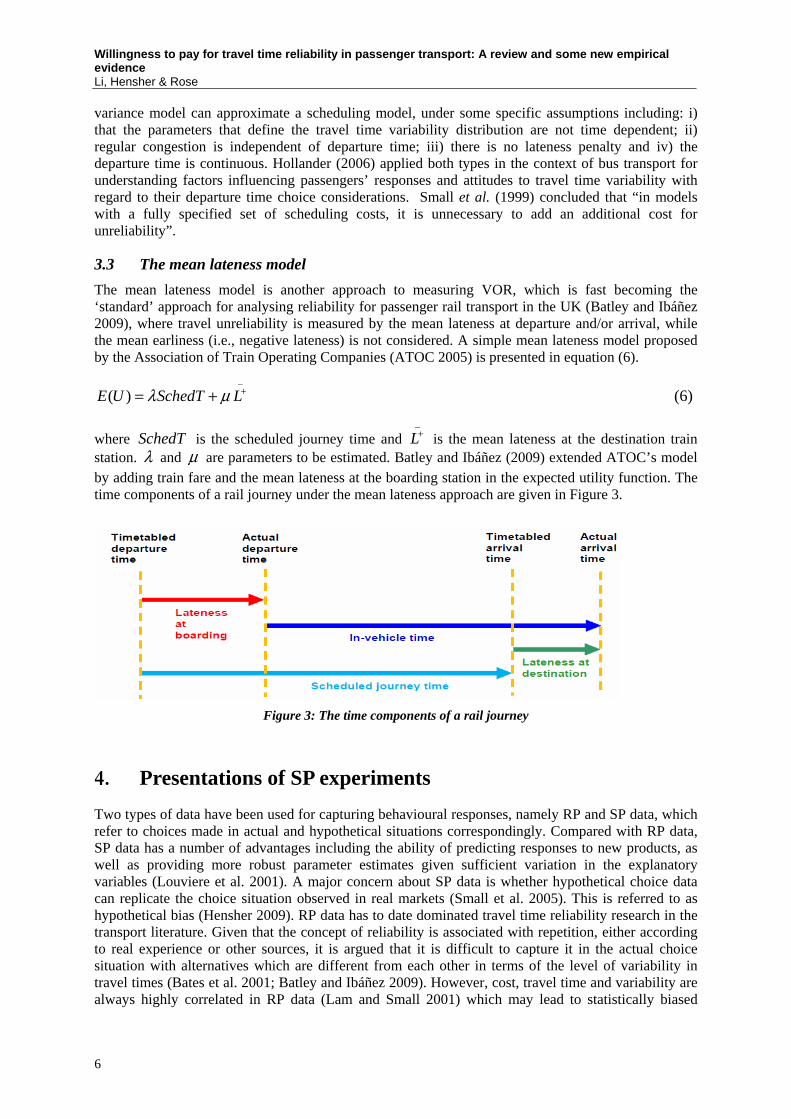
The mean lateness model is another approach to measuring VOR, which is fast becoming the ‘standard’ approach for analysing reliability for passenger rail transport in the UK (Batley and Ibáñez 2009), where travel unreliability is measured by the mean lateness at departure and/or arrival, while the mean earliness (i.e., negative lateness) is not considered. A simple mean lateness model proposed by the Association of Train Operating Companies (ATOC 2005) is presented in equation (6).

_

( )E U SchedT Lλ μ += + (6)

where is the scheduled journey time and SchedT_

L+ is the mean lateness at the destination train station. λ and μ are parameters to be estimated. Batley and Ibáñez (2009) extended ATOC’s model by adding train fare and the mean lateness at the boarding station in the expected utility function. The time components of a rail journey under the mean lateness approach are given in Figure 3.

Figure 3: The time components of a rail journey

4. Presentations of SP experiments

Two types of data have been used for capturing behavioural responses, namely RP and SP data, which refer to choices made in actual and hypothetical situations correspondingly. Compared with RP data, SP data has a number of advantages including the ability of predicting responses to new products, as well as providing more robust parameter estimates given sufficient variation in the explanatory variables (Louviere et al. 2001). A major concern about SP data is whether hypothetical choice data can replicate the choice situation observed in real markets (Small et al. 2005). This is referred to as hypothetical bias (Hensher 2009). RP data has to date dominated travel time reliability research in the transport literature. Given that the concept of reliability is associated with repetition, either according to real experience or other sources, it is argued that it is difficult to capture it in the actual choice situation with alternatives which are different from each other in terms of the level of variability in travel times (Bates et al. 2001; Batley and Ibáñez 2009). However, cost, travel time and variability are always highly correlated in RP data (Lam and Small 2001) which may lead to statistically biased

6


Li, Hensher & Rose

estimates. Bates et al. (2001, p.214) considered that SP is the preferred option for collecting data on travel time reliability.4

In early SP experiments, travel time variability was often presented as the extent and frequency of delay relative to normal travel time (which we refer as a Type 1 experiment). An example to estimate the trade-off between travel time and variability is given in Table 1, from Jackson and Jucker (1982), where respondents are asked to make a choice between a journey that always takes 30 minutes and a journey which has a shorter time, but a possibility of 5-minute delay once a week. In this type of experiment, travel time variability is shown in an implicit manner, and it is difficult for respondents to fully understand and interpret specific features of the travel time distribution from it.

Table 1: SP task from Jackson and Jucker (1982)

Card Route 1 Route 2 Usual time: 30 minutes 20 minutes 1 Possible delays: None 5 minutes a week

More recent reliability studies have included a series of arrival times (normally five or 10 levels) in their SP experiments (Type 2) to capture time variability (see, e.g., Senna 1994; Noland and Small 1995; Small et al. 1999; Hollander 2006; Asensio and Matas 2008; Batley and Ibáñez 2009). Hamer et al. (2005) suggested that travel time variability should be presented as a series of travel times associated with each alternative in the SP experiment. A general concern about this approach is that respondents may neglect some attributes, if the amount of information to process results in cognitive burden. Although it is widely accepted that a series of travel times should be presented, two recent studies retained the traditional approach in their SP experiments based on the extent and frequency of delay (see e.g., Small et al. 2005; Brownstone and Small 2005). The SP choice examples for the mean-variance model, the scheduling model, and the mean lateness model with multiple travel information for each alternative are presented below.

An SP choice set from Senna (1994) is shown in Table 2, where one route has no travel time variability on five occasions, while the alternative route has different levels of mean travel times and variability, along with cost. The choice response is sought from a 5-point semantic scale. Travel time variability in model estimation is defined by the standard deviation of travel time (i.e., the mean-variance model).

Table 2: A SP task from Senna (1994), the mean variance model

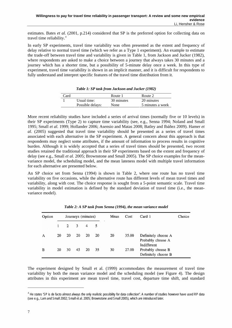
The experiment designed by Small et al. (1999) accommodates the measurement of travel time variability by both the mean variance model and the scheduling model (see Figure 4). The design attributes in this experiment are mean travel time, travel cost, departure time shift, and standard

4 He states ‘SP is de facto almost always the only realistic possibility for data collection”. A number of studies however have used RP data (see e.g., Lam and Small 2002; Small et al. 2005; Brownstone and Small 2005), which are introduced later.

7

Willingness to pay for travel time reliability in passenger transport: A review and some new empirical evidence Li, Hensher & Rose deviation of travel time, while the attributes shown to respondents are mean travel time, travel cost, and five equi-probable arrival scenarios (early, late or on time) with respect to the preferred arrival time. For the mean-variance model, the standard deviation of travel time is calculated as equation (7).

52

1

1( ) [ ( )]5 i

iSD T X E X

=

= − (7)

where iX is five schedule delay values for each alternative. The example values for Option A in Figure 5 are -7, -4, -1, 5 and 9. For the scheduling model, the lateness probability is the chance of being late out of five arrivals. For example, it is 0.4 for Choice A in Figure 5, and the expect values for SDE and SDL are:

(7 4 1 0 0) (0 0 0 5 9)E(SDE) 2.4;E(SDL) 2.85 5

+ + + + + + + += = = = . (8)

Figure 4: SP task from Small et al. (1999)

Batley and Ibáñez (2009) employed the mean lateness model. Compared with the scheduling model, the difference is that the mean lateness model only considers the scenarios of being late at both the departure and destination relative to the scheduled timetable; while the scheduling model addresses both early and late arrival with respect to the preferred arrival time. In Batley and Ibáñez’s SP experiments (see Figure 5), two train travel options for a given journey are presented in terms of fare, scheduled journey time and the distribution of journey time (shown as five events of train travel). The probabilities of these five events are not shown to respondents, which are assumed to be equi-probable for analysis. Four design variables are constructed: cost, timetabled journey time, departure time variation and journey time variation. Departure time variation has three levels of lateness at the boarding station and three levels of journey time were established around the scheduled travel time, which together created the late arrival times at the destination.

8


Li, Hensher & Rose

Figure 5: An SP task from Batley and Ibáñez (2009), the mean lateness model

The surveys shown above ask respondents to choose the preferred alternative among a number of alternatives associated with different levels of attributes. Another way of obtaining choice information is by ranking. Bates et al. (2001) designed an SP experiment (see Figure 6) in which respondents were presented two train operators with different fares, different timetables, and different combinations of 10 possible arrivals (early or late) at the destination in terms of the clockface of cards for each alternative. Each respondent was given six sets of choices and asked to rank the four best alternatives out of the six combinations. The clockface presentation was designed to overcome a problem when travel time information is shown as a sequence. That is, respondents may assume the order is descending or ascending and hence overlook the entire sequence (Hollander 2006).

Figure 6: A SP task from Bates et al. (1999)

Using face-to-face interviews (30 interviewees in total), Tseng et al. (2009) evaluated the above representations of travel time variability including i) verbal description (see e.g., Small et al. 1999), ii) clock-face presentation (Bates et al. 2001), and iii) vertical bars (see e.g., Batley and Ibáñez 2009) in order to find out how consistently and logically respondents understood the concept of variability, based on five key indicators: i) clearness of the presentation of reliability, ii) ease of making choice between two alternatives/trips, iii) ease of considering all information/attributes, iv) attractiveness of

9


10

the visual appearance, and iv) ease of answering the test questions. Their comparison shows that verbal description performed best, followed by vertical bars and clock-bar presentations.

Given that i) multiple travel times for each alternative have been given in the SP experiments to reflect the stochastic nature of travel time; ii) the verbal description is the best representation to describe travel time variability in SP experiments (Tseng et al. (2009); and iii) it is capable of estimating both the scheduling model and the mean-variance, the experiment by Small et al. (1999) is considered to still be best practice among our reviewed travel time reliability SP designs.

Some recent SP experiments for travel time reliability are summarised in Table 3.

Table 3: A summary of SP experiments for valuing travel time reliability

Study Structure Information shown in Survey Presentation of variability in Survey Attributes in utility function

Senna (1994) Mean-variance Travel cost, mean travel time,

travel time variability Five different travel times for each

alternative Cost, travel time, variability

Small et al. (2005) Mean-variance Toll, travel time the frequency of

being delayed 10 minutes+ Frequency of being delayed 10 minutes or

more for each alternative Cost, travel time, variability

Brownstone & Small (2005) Mean-variance Toll, travel time, the frequency of

being delayed 10 minutes+ Frequency of being delayed 10 minutes or

more for each alternative Cost, travel time, variability

Noland et al. (1998) Scheduling

Departure time before the usual arrival time, mean travel time,

travel time variation Five different travel times for each

alternative

Expected travel time, E(SDL),E(SDE), the probability of being late arrival, standard deviation, coefficient of

variation (standard deviation divided by mean travel time)

Bates et al. (2001) Scheduling

Fare, scheduled departure time and arrival time, preferred arrival

time, variation in arrival time

10 arrival scenarios (minutes late, early or late) in a clock face format for each

alternative

Cost, headway, mean difference between actual arrival and scheduled

arrival times, E(SDE), E(SDL),

Holland (2006) Scheduling Fare, preferred arrival time,

travel time variation Five different travel times shown by five

vertical bars for each alternative Cost, expected travel time,

E(SDL),E(SDE), standard deviation

Asensio & Matas (2008) Scheduling

Travel cost, mean travel time, arrival time variations

Five arrival scenarios (minutes late or early) for each alternative

Cost, expected travel time, E(SDL),E(SDE), the probability of

being late arrival

Batley & Ibáñez (2009) Mean lateness

Fare, timetabled journey time, departure time variation and

journey time variation

Five travels (differences in departure times and travel times hence in arrival times) shown by five vertical bars for

each alternative

Cost, timetabled journey time, mean lateness at the origin and mean lateness

at the destination

Small et al. (1999) Mean-variance &

Scheduling Toll, average travel time, variation in arrival times

Five arrival scenarios (minutes late, early or on time) for each alternative

Cost, mean travel time, standard deviation, E(SDL),E(SDE), the probability of being late arrival

Note: Small et al. (2005) and Brownstone & Small (2005) have used both RP and SP.


5. Recent travel time variability valuation studies

The majority of empirical research for analysing and estimating VOR is established on SP data, by asking respondents to make choices under hypothetical scenarios to reveal their behavioural responses to this attribute. Bates et al. (2001) estimated rail passengers’ VOR in the UK. They included 10 possible travel times for each alternative, with the expected values of SDE and SDL calculated over the 10 possible arrivals (assumed to be equi-probable). The estimate for the expected SDE is £33.6 (US$ 66.7)5 per hour and £68.2 ($US135.4) per hour for the expected SDL. However there is no variation in the scheduled travel time variable between alternatives in the SP experiment, hence the parameter for travel time cannot be estimated directly. Instead, the mean arrival lateness (i.e., the mean difference between arrival time and scheduled arrival time) is included in the model, which is £76.0 ($US150.9) per hour.

Bates et al. (2001) define total travel time ( ) in terms of free flow time (( )htT fT ), congestion

time ( xT

ht), and travel time variability ( ), with the last two elements dependent on departure

time ( ). rT

h hf x rt tT( ) T T T ( )( )= + + ht

(9)

Although total time consists of several components, most studies aggregate the first two time components in equation (9) into a single variable when estimating travellers’ values of travel time savings. As far as we know, toll road studies undertaken by Hensher produced the earliest estimates for each component of time. For example, Hensher (2001a) investigated the values of different time components in the context of long distance car travel (up to three hours) in New Zealand. He further divided congestion time into slowed down time and stop/start time. Under the MNL model, his estimate of VTTS is NZ$3.6 ($US3.7) per hour for free flow time, NZ$12.9 ($US13) per hour for slowed down time and NZ$27.8 ($US28.1) per hour for stop/start time, and the VOR (measured by uncertainty in his experiment) is NZ$5 ($US4.9) per hour.

The above two studies using SP data are illustrative of many empirical studies interested in VOR. For example, Asensio and Matas (2008) applied the scheduling model to understand Spanish car drivers’ responses to travel time variability, and found that drivers are willing to pay more for reducing the time of arriving late than for the equivalent reduction in the mean travel time (Euro 34.4 ($US 53.9) per hour vs. Euro14.1 (US$22.1) per hour), while the willingness-to-pay for the reduction in early arrival is the lowest (Euro 7.0 ($US11) per hour). Hollander (2006) found similar evidence for bus commuters in the UK, concluding that the scheduling model has an improved statistical performance over the mean-variance model. Batley and Ibáñez (2009) found that the value of reliability (measured by the standard deviation of travel time) is more than twice the VTTS for rail passengers in the UK.

Some USA studies have used RP data to analyse drivers’ responses to congestion pricing, mainly on two roads in the USA, State Route 91 (SR 91) and the Interstate 15 (I-15). These routes offered two distinctive congestion pricing schemes; SR91’s express lanes vary tolling prices according to the schedule which are different at times of day, days of week and Eastbound or Westbound; while the express lanes on I-15 implemented “dynamic pricing” in which toll tariffs vary in real time to avoid congestion. Drivers may also use free lanes to avoid the toll and have to contend with time delays.

For the analysis of SR 91, both travel time and time variability are considered (see e.g., Lam and Small 2001; Small et al. 2005), while the I-15 studies are focused on values travel time

5 All $US figures are from Table 5 and refer to 2009 dollars.

12


savings (see e.g., Brownstone et al. 2003; Steimetz and Brownstone 2005). The framework of these RP studies for VOR is similar to the mean-variance model, but with different measures of travel time variability and the travel time. In the mean-variance model, the travel time variable is the mean time; however the RP studies use the median of the observed travel time distribution in the utility function. Instead of using the standard deviation, travel time variability is measured either by the difference between the 90th and the 50th percentiles of the travel time distribution (see e.g., Lam and Small 2001), or the difference between the 80th and the 50th percentiles (see e.g., Small et al. 2005). Using the median and the difference between percentiles improves the log-likelihood ratio compared with the value when using the mean and the standard deviation (Lam and Small 2001).

Small and his colleagues also used SP experiments (see e.g., Small et al. 2005; Small and Brownstone 2005) sampling three groups of people using the SR 91 motorway. They began with an RP telephone survey of 438 respondents undertaking commuting and other trip purposes. The second and third samples are follow up mail surveys, where the first stage collected RP information on actual trips, and the second stage presented eight SP scenarios to respondents (55 of whom also answered the RP questions during the first stage). The pooled sample consisted of 522 RP observations and 633 SP observations from 81 respondents.

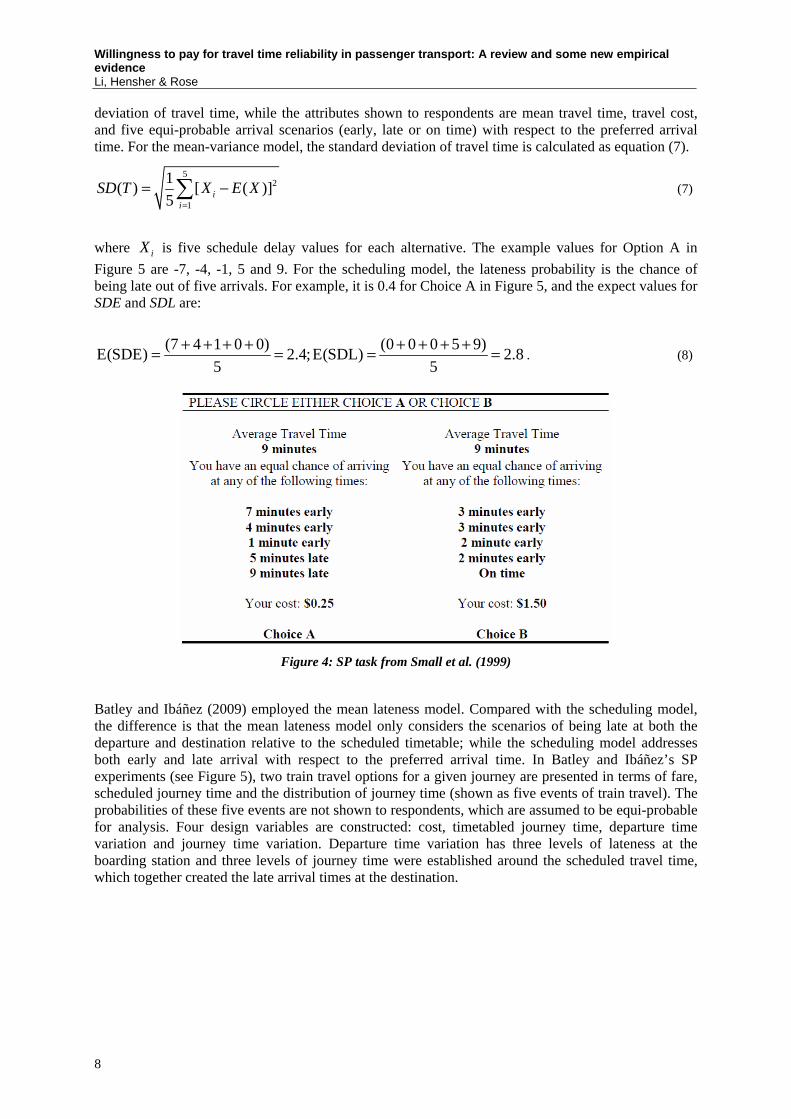
In order to construct RP variables, travel information on the free lanes of SR 91 was collected on 11 different days, and local linear regression was used to smooth data and to estimate the mean and percentiles of the distribution at different times between 6am and 10am. It is assumed that the travel time for using tolled lanes is constant (eight minutes). The estimated median time savings and reductions in variability from tolled lanes relative to using free lanes are shown in Figure 7.

Figure 7: Estimated time benefits of using tolled lanes

For the RP setting, travel time is presented by the median of the actual distribution, while the unreliability of travel time is measured by the difference between the 80th and the 50th percentiles. For the SP setting, each respondent answered eight choice sets with the similar variables to those in the RP survey. In their SP experiments (see Table 4), travel time variability is shown as the frequency of being late at the destination by 10 minutes or more. One limitation of this SP design is that it cannot produce the VOR per hour, given the probabilistic formulation. For example, using their SP data, Small et al. (2005) estimated the median value of reliability as US$5.40 per incident. That is, the median motorist in their sample is willing to pay US$0.54 per trip to reduce the probability of over a 10-minute delay by 10 percent.

13


Table 4: An SP example question for SR 91 (Small et al. 2005)

One reason that RP techniques are applicable is that those studies are conducted in an environment where two types of lanes (free and tolled) are co-existing. If the route choice is more complicated than this, it becomes difficult to use RP to present clearly the variability variable to respondents. The early studies on the SR 91 corridor by Small and his colleagues relied on SP data, before RP information was available.6

The SP data in Small et al. (1999) were collected in 1995; the number of observations is 5,630 for the mean-variance model, and 5,624 for the scheduling model. In their mean-variance model (referred to as Model 11), the average VTTS is US$3.9 per hour and the VOR is US$12.6 per hour. That is, a reliability ratio of 3.3. For the scheduling model (Model 15), the VTTS value is $US3.4 per hour, and the monetary value of expected SDL is US$18.6 per hour. The SDL ratio (i.e., the value of expect SDL divided by the value of time) is 5.5, higher than the reliability ratio. Small et al. (1999) also investigated non-linearity in the value of SDE. That is, when SDE =5 minutes, the marginal value is US$0.028 per minute (US$1.7/h); when it increases to 10 minutes, the SDE value rises to US$0.078 per minute (US$4.7/h). Their findings are supported by the theory of bands of indifference (see Mahmassani and Chang 1986). Mahmassani and Chang found that there is no schedule disutility perceived by travellers if the arrival is within 5 minutes of the preferred arrival time.

More recent studies on SR 91 prepared by Small and his colleagues have focussed on a mixture of RP and SP data, comparing the results from RP and SP. For example, according to Small et al. (2005), the estimated VTTS value is US$21.5 per hour using the RP data, and US$12.0 per hour from the SP model, while the value of reliability is US$19.7 per hour based on RP and US$5.4 per incident based on SP data. Therefore, they concluded that SP studies underestimate the value of time savings, compared to the evidence using RP data. Hensher (2009) investigates this assertion in some detail and suggests that part of the difference may be due to the way in which the SP data is used in model estimation.

5.1 Comparison of a series of reliability studies on SR 91

Given that the contributions by Ken Small and his colleagues are generally regarded as best practice, we compare the three recent empirical studies on SR 91 in order to identify key sources influencing their estimates (see Small et al. 1999; Small et al 2005 and Brownstone and Small 2005 summarised in Table 5). All three studies focussed on the car commute, with the mean-variance model applied when using SP data . However, the estimated time values7 6 The express lanes on SR91 were constructed in the late 1995. Lam and Small (2001) is one of the initial studies which used information on actual travel behaviour, by observing drivers’ actual choices between free lanes and express lanes on SR91. Only RP was used in Lam and Small (2001) for valuing travel time savings and reliability.

7 The scheduling model is also used in Small et al. (1999). Also Brownstone and Small (2005) have RP and SP, however the model is estimated based on SP only.

14


are significantly different between the study published in 1999 and the papers published in 2005.

The VTTS estimate from Small et al. (2005), based on SP data, is almost triple the estimate from Small et al. (1999) (SP only) (US$11.9 per hour vs. US$3.9 per hour). The key differences between these two studies are: i) the data collection period (1999-2000 for Small et al. (2005) vs. 1995 for Small et al. (1999)), ii) the choice model (mixed multinominal logit (MMNL) vs. the multinominal logit (MNL)), iii) the number of respondents and observations, and iv) the way of presenting travel time variability in experiments. By dividing the VTTS by the average hourly wage at corresponding periods, we can neutralise the impact of different data collection periods (income, inflation, etc.). The average wage for respondents surveyed in 1995 was US$19.2 per hour, and the average wage from the other study was US$23.1 per hour8. Hence, the VTTS ratio relative to the average wage rate is 20.3 percent for Small et al. (1999) and 54.5 percent for Small et al. (2005). After removing the impact of the period of data collection, the estimates from two studies remain significantly different. That is, the year is a marginal contributor to the difference9.

Although there are some differences between these two papers published in 2005 including (1) the numbers of respondents/observations, and (2) choice model specification, the estimated values (SP) are similar (e.g., VTTS: US$11.9 per hour vs. US$12.6 per hour; value of reliability: US$5.4 per incident vs. US$5.0 per incident). Hence, the differences in (1) and (2) have not resulted in significantly different values of travel time savings and reliability between the two studies.

The above analysis suggests that the way of presenting time variability may be the key contributor to different VTTS estimates between Small et al.’s papers in 1999 and 2005. In their early paper (1999), travel time variability was verbally described in the SP experiments by five arrival scenarios (minutes late, early or on time) for each alternative (see Figure 4); however in Small et al. (2005) travel time variability was shown as the frequency of being delayed 10 minutes or more for each alternative. The experiment with multiple travel times for each alternative is arguably, better understood and more appropriate to capture the concept of travel time variability, which has been widely used in recent reliability studies, especially after 2000. Also, the evaluation of different travel time variability representations with multiple travel times by Tseng et al. (2009) suggested that the verbal description is the best way to present time variability in SP surveys. Hence, theoretically, the estimated value of reliability from Small et al. (1999) is potentially more robust. We suggest that the change in the representation of trip time variability is the major contributing influence on the differences in respondents’ perceptions of travel time reliability. Given that the value of travel time reliability also has an impact on the value of travel time savings (see Senna 1994), we can also expect to see variations in VTTS estimates (US$3.9 per hour or 20.3 percent of hourly average wage in Small et al. (1999) vs. US11.9 per hour or 54.5 percent of hourly wage in Small et al. (2005)).

Table 5 summarises recent empirical studies10 that obtained estimates of values of travel time reliability and time savings. To present a more informative picture of which method tends to produce higher or lower estimates, we also provide reliability ratios across different studies in ascending order (Figure 8). The advantage of using the ratio of reliability instead of using the value of reliability is we can control for the influence of location, currency, inflation, etc. The 8 We cannot compare the values of reliability from those two studies, given different units (per hour and per incident) due to the design. 9 Tseng (2008) undertook a meta analysis of values of travel time variability and found that time trend has no significant impact. In Tseng’s meta analysis, potential sources of systematic differences include the trip purpose, the presence of unobserved heterogeneity, and the form of the utility specification. 10 The reliability ratio estimated from Hollander (2006) is not considered, given that it is strangely (0.1), given that the ratio for public transport should between 1.4 and 2.0 (de Jong et al. 2009; Bates et al. 1999).

15


16

evidence suggests that the type 2 design (in which a series of travel times are presented for each alternative) produces higher reliability ratios than the simpler type 1 design; and rail travel has a higher reliability ratio than car. Although vertical bars were used for valuing reliability of rail in Batley and Ibáñez (2009) only, we believe the higher ratio is mostly due to the characteristics of public transport (e.g., given the fixed service intervals (timetable), a public transport user’s choice is limited; while however a car driver has more flexibility such as the adjustment of departure time. Hence, the consequence of being unreliable is more serious in the context of public transport which leads to more uncertainty or cost, such as waiting for the next service (unreliable departure time), missing the next connection (lateness in travel time, etc.) which leads to a higher ratio (see e.g., de Jong et al. 2009) rather than the way that reliability is presented (i.e., verbal or bars). Whether SP overestimates or underestimates the ratio is unclear, supported by the meta analysis of Tseng (2008).


Study

Date collection

period Mode

Location Trip purpose Data #Respondents #Observations Value of time

savings Value of reliability* Value of SDE Value of SDLValue of

Lateness(i) Value of

Lateness(j)

Bates et al. (2001) n/a Rail UK n/a SP 28 672 n/a n/a £33.6/h

$09US: 66.7 £68.2/h

$09US: 135.4 n/a £76.0/h

$09US: 150.9

Hensher (2001a) 1999 Car NZ long-distance

(<3hours) SP 198 3168 NZ$ 8.7/h

$09US: 8.6 NZ$ 5.0/h

$09US: 4.9

n/a

n/a

n/a

n/a

Hollander (2006) 2004 Bus UK Commute SP 244 2165 £4.2/h

$09US: 7.9 £0.42/h

$09US: 0.79 £3.1/h

$09US: 5.9 £8.6/h

$09US: 16.3 n/a n/a

Asensio & Matas (2008) n/a Car Spain Commute SP 259 2331

€ 14.1/h $09US: 22.1 n/a

€ 7.0 $09US: 11.0

€ 34.4 $09US: 53.9 n/a n/a

Batley & Ibáñez (2009) 2007 Rail UK

Commute (mainly) SP 2395 11763

£15.4/h $09US: 27.3

£31.8/h $09US: 56.4 n/a n/a

£19.2/h $09US: 34.0

£55.9/h $09US: 99.1

Small et al. (1999) 1995 Car US (SR91) Commute (mainly) SP n/a

5630 (mean-variance)

5624 (scheduling)US$3.9/h

$09US: 5.1 US$12.6/h

$09US: 17.8 Non-linear US$18.6/h

$09US: 26.2 n/a n/a

Lam & Small (2001) 1997&1998 Car US (SR91) n/a RP 332 332 US$22.9/h

$09US: 30.5

US$15.1/h (Male) $09US: 20.1

US$31.9/h (female) $09US: 42.5 n/a n/a n/a n/a

Small et al. (2005) 1999&2000 Car US (SR91) Commute (mainly) RP/SP 548 1155

US$21.5/h (RP) $09US: 27.5;

US$11.9/h (SP) $09US: 15.2

US$19.6(RP); $09US: 25.0

US$5.4/incident(SP) $09US: 6.9 n/a n/a n/a n/a

Brownstone & Small (2005) 1999&2000 Car US (SR91) Commute (mainly) RP/SP 81 601

US$12.6/h (SP)

$09US: 16.1 US$5.0/incident(SP)

$09US: 6.4 n/a n/a n/a n/a

Bhat & Sardesai (2006) n/a

Multi-modes US Commute RP/SP 679 1955

US$12.2/h $09US: 13.3

US$3.3/h (with flexible arrival time)

$09US: 3.6; US$ 6.1/h (with inflexible

arrival time) $09US: 6.6

n/a n/a n/a n/a

Table 5: A summary of some recent valuation of travel time reliability studies

Notes:

Reliability*: standard deviation for SP or differences between 90th or 80th percentile and the median of travel time for RP Value of Lateness(i): value of mean lateness at boarding Value of Lateness(j): value of mean lateness at destination $09US: the values are all converted into US dollars based on the current exchange rates (23 October 2009) and inflated to 2009 based on CPI (i.e., US$2009) Multi-mode: Bhat and Sardesai (2006) include car (drive alone and shared ride), car and rail in their SP.

17


18

Notes: Type 1: Single travel time for each alternative Type 2: Multiple travel times for each alternative Reliability ratio: the marginal rate of substitution between average travel time and travel time variability (i.e., SD T/β β ) Multi-mode: Bhat and Sardesai (2006) include car (drive alone and shared ride), car and rail in their SP.

Figure 8: Values of reliability ratios across studies


Li, Hensher & Rose

19

6. New empirical evidence: An Australian case study

A number of WTP studies have been undertaken in Australia in the context of toll vs. free roads, some of which have addressed the valuation of travel time reliability. The most recent study, undertaken in 2008, presented three travel scenarios in eight stated choice scenarios - ‘arriving x minutes earlier than expected’, ‘arriving y minutes later than expected’, and ‘arriving at the time expected’. Each is associated with a corresponding probability of occurrence to indicate that travel time is not fixed but varied from time to time (see Table 6). For all attributes except the toll cost, minutes arriving early and late, and the probabilities of arriving on-time, early or late, the values for the stated choice (SC) alternatives are variations around the values for the current trip. Given the lack of exposure to tolls for many travellers in the study catchment area, the toll levels are fixed over a range, varying from no toll to $4.2011, with the upper limit determined by the trip length of the sampled trip. The variations used for each attribute are given in Table 6.

Table 6: Profile of the Attribute range in the SC design

Attribute Level 1 Level 2 Level 3 Level 4 Level 5 Level 6 Level 7 Level8 Free Flow time -40% -30% -20% -10% 0% 10% 20% 30% Slowed down time -40% -30% -20% -10% 0% 10% 20% 30% Stop/Start time -40% -30% -20% -10% 0% 10% 20% 30% Min. Early 5% 10% 15% 20% - - - - Min. Late 10% 20% 30% 40% - - - - Prob arriving Early 10% 20% 30% 40% - - - - Prob arriving On-time 20% 30% 40% 50% 60% 70% 80% - Prob arriving Late 10% 20% 30% 40% - - - - Running costs -25% -15% -5% 5% 15% 25% 35% 45% Toll costs $0.00 $0.60 $1.20 $1.80 $2.40 $3.00 $3.60 $4.20

A survey was designed and implemented in late 2008 to capture a large number of travel circumstances, to determine how each individual trades-off different levels of travel times and trip time reliability with various levels of proposed tolls and vehicle running costs, in the context of tolled and non-tolled roads. Sampling rules were imposed on three trip length segments: 10 to 30 minutes, 31 to 45 minutes, and more than 45 minutes (capped at 120 minutes). Sampling by the time of day that a trip commences was also included, defining the peak12 as trips beginning during the period 7-9 am or 4.30-6.30pm. All non-peak trips are treated as off peak in the internal quota counts.

There are three versions of the experimental design depending on the trip length, with each version having 32 choice situations (or scenarios) blocked into two subsets of 16 choice situations each. In generating the designs, the free flow, slowed and stop/start times were set to five minutes if the respondent entered zero for their current trip. It is important to understand that the distinction between free flow, slowed down and stop/start/crawling time is solely to promote the differences in the quality of travel time between various routes – especially a tolled route and a non-tolled route, and is separate to the influence of total time. An example of a choice scenario is given in Figure 9. The first alternative is described by attribute levels associated with a recent trip; with the levels of each attribute for Routes A and B pivoted around the corresponding level of actual trip alternative.

In total, 280 commuters were sampled for this study. McFadden (1984, page 1442) suggests:

“As a rule of thumb, sample sizes which yield less than thirty responses per alternative produce estimators which cannot be analyzed reliably by asymptotic methods”.

11 The range was provided on advice from a consortium of bidders for the right to build and operate a toll road under a long term concession agreement. 12 The way we handle trips that are partly in the peak: a trip is peak if 60 percent or more of the trip falls within the peak period.


20

This indicates that the sample size used herein is more than adequate in accommodating the variability required in the choice responses across the alternatives, to obtain asymptotically efficient parameter estimates. In addition, the experimental design method of D-efficiency used herein is specifically structured to increase the statistical performance of the models with smaller samples than are required for other less-(statistically) efficient designs, such as orthogonal designs (see Rose and Bliemer 2008).

An example of the choice experiment is given in Figure 11. The first alternative is described by attribute levels associated with a recent trip; with the levels of each attribute for Routes A and B pivoted around the corresponding level of the revealed preference alternative. The sample population included commuting and non-commuting car travel, and each respondent answered 16 choice sets.

Figure 9: Illustrative stated choice screen

The choice design allows us to estimate the mean-variance model (where variability is represented by the standard deviation of travel time), and the scheduling model (expected schedule delay early and late (ESDE and ESDL)) for travel time variability. Multinominal logit (MNL) and mixed multinomial logit (MMNL) models are estimated , and modelling results for commuters and non-commuters under the scheduling model and mean-variance model are shown in Table 7. We investigated normal and triangular distributions for the random parameters and found an improved model fit when using the triangular distribution. All estimated parameters for the REF (status quo) specific constant are positive, which suggest, after accounting for the observed influences, that sampled respondents prefer their current trip relative to two stated choice alternatives. The mean-variance model delivers slightly

13 14

13The constrained triangular distribution was used for the random parameters (average travel time, standard deviation of travel time, ESDE and ESDL). Let c be the centre and s the spread. The density starts at c-s, rises linearly to c, and then drops linearly to c+s. It is

zero below c-s and above c+s. The mean and mode are c. The standard deviation is the spread divided by 6 ; hence the spread is the

standard deviation times 6 . The height of the tent at c is 1/s (such that each side of the tent has area s×(1/s)×(1/2)=1/2, and both sides have area 1/2+1/2=1, as required for a density). The slope is 1/s2. For a constrained distribution, the mean parameter is constrained to equal its spread (i.e., βjk = βk + |βk| Tj , and Tj is a triangular distribution ranging between -1 and +1), and the density of the distribution rises linearly to the mean from zero before declining to zero again at twice the mean. Therefore, the distribution must lie between zero and some estimated value (i.e., the βjk). The mean and standard deviation is the same under a constrained triangular distribution..

14 Models were estimated using Nlogit4. Starting values for mixed logit are MNL values. The convergence criteria is the gradient g’Hg<εg where g is the current derivative vector and H is the inverse of the current Hessian.


Li, Hensher & Rose

better model fit than the scheduling model under both MNL and MMNL for commuters, while the opposite results occurs for non-commuters

The WTP estimates of interest summarised in Table 8, treating the components of travel time as a single total time as well as aggregating the cost components; namely the value of travel time savings (VTTS = time cos t/β β ), the value of reliability (VOR = Stan Dev cos t/β β ), the value of expected schedule delay early (ESDE = ESDE cos t/β β ), and the value of expected schedule delay late (ESDL = ESDL cos t/β β ), along with reliability ratios (VOR/VTTS, ESDE/VTTS and ESDL/VTTS).

Table 7a: MNL and MMNL modelling results for commuters (4,696 observations)

MNL

Scheduling Mean-variance Variable Parameter t-ratio Variable Parameter t-ratio

REF 1.0697 19.1 REF 1.0621 19.4 TIME -0.0680 -16.4 TIME -0.0681 -16.5 COST -0.1798 -10.1 COST -0.1814 -10.6 ESDE -0.0870 -2.0 STANDEV -0.1085 -4.8 ESDL -0.1112 -4.8 AIC15 7012.8 AIC 7008.8

Log-likelihood -3500.54 Log-likelihood -3498.78 MMNL


Nonrandom parameters: Nonrandom parameters: REF 1.0764 18.4 REF 1.0663 21.3

COST -0.2023 -10.6 COST -0.2404 -24.1 Means for random parameters: Means for random parameters:

TIME -0.1091 -15.8 TIME -0.1252 -18.6 ESDE -0.0816 -1.7 STANDEV -0.1629 -6.5 ESDL -0.1316 -5.2

Standard deviations for random parameters: Standard deviations for random parameters:

TIME 0.1091 15.8 TIME 0.1252 18.6 ESDE 0.0816 1.7 STANDEV 0.1629 6.5 ESDL 0.1316 5.2 AIC 6838.9 AIC 6679.4

Log-likelihood -3413.42 Log-likelihood -3383.10 Notes:

MMNL: simulation based on 50 Halton draws, constrained triangular distribution

15 Akaike information criterion: AIC=-2×log-likelihood + 2×K , where K is the number of parameters. The smaller AIC indicates a better model fit.

21


22

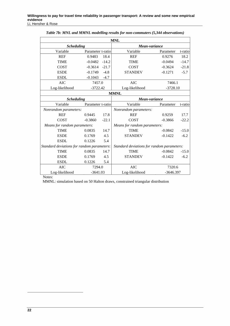
Table 7b: MNL and MMNL modelling results for non-commuters (5,344 observations)

MNL


REF 0.9483 18.4 REF 0.9276 18.2 TIME -0.0482 -14.2 TIME -0.0494 -14.7 COST -0.3614 -21.7 COST -0.3624 -21.8 ESDE -0.1749 -4.8 STANDEV -0.1271 -5.7 ESDL -0.1043 -4.7 AIC 7457.0 AIC 7466.1

Log-likelihood -3722.42 Log-likelihood -3728.10 MMNL


Nonrandom parameters: Nonrandom parameters: REF 0.9445 17.8 REF 0.9259 17.7

COST -0.3860 -22.1 COST -0.3866 -22.2 Means for random parameters: Means for random parameters:

TIME 0.0835 14.7 TIME -0.0842 -15.0 ESDE 0.1769 4.5 STANDEV -0.1422 -6.2 ESDL 0.1226 5.4

Standard deviations for random parameters: Standard deviations for random parameters: TIME 0.0835 14.7 TIME -0.0842 -15.0 ESDE 0.1769 4.5 STANDEV -0.1422 -6.2 ESDL 0.1226 5.4 AIC 7294.0 AIC 7320.6

Log-likelihood -3641.03 Log-likelihood -3646.397 Notes:

MMNL: simulation based on 50 Halton draws, constrained triangular distribution


Li, Hensher & Rose

Table 8: Values of time savings and reliability, and scheduling costs for commuters and non-commuters ($Aud2008 per person hour)

Survey A

Commuter Non-commuter Scheduling Scheduling

MNL MMNL MNL MMNL VTTS (mean) 22.69 30.04 VTTS (mean) 8.01 12.22 VTTS (StDev) n/a 10.22 VTTS (StDev) n/a 3.64 ESDE (mean) 29.04 24.10 ESDE (mean) 29.03 27.31 ESDE (StDev) n/a 0.80 ESDE (StDev) n/a 1.52 ESDL (mean) 37.10 38.86 ESDL (mean) 17.32 18.98 ESDL (StDev) n/a 2.52 ESDL (StDev) n/a 1.18 ESDE/VTTS 1.28 0.80 ESDE/VTTS 3.62 2.23 ESDL/VTTS 1.64 1.29 ESDL/VTTS 2.16 1.55

Log likelihood -3500.54 -3413.42 Log likelihood -3722.43 -3641.03 No. of obs. 4496 No. of obs. 5344

Mean-variance Mean-variance MNL MMNL MNL MMNL

VTTS (mean) 22.52 28.28 VTTS (mean) 8.18 12.31 VTTS (StDev) n/a 10.59 VTTS (StDev) n/a 3.68 VOR (mean) 35.87 40.39 VOR (mean) 21.04 21.91 VOR (StDev) n/a 3.32 VOR (StDev) n/a 1.40 VOR/VTTS 1.59 1.43 VOR/VTTS 2.57 1.78

Log likelihood -3498.78 -3383.10 Log likelihood -3728.10 -3646.40 No. of obs. 4,496 No. of obs. 5,344

Note: VOR: measured by the standard deviation

We focus only on the mixed logit results.16 For commuters, under the scheduling model, the value of ESDL is $38.86/hour, which suggests that individuals are willing to pay a substantial amount to avoid the consequence (or cost) of being late to work. The mean VTTS is $30.04/hour and the mean ESDE is$24.1/hour, giving a ratio for ESDE/VTTS of 0.8, which is in line with previous studies (e.g., 0.74 for Hollander (2006) and 0.5 for Asensio and Matas (2008). Under the mean-variance model, the VTTS estimates are similar to the estimates from the scheduling model. According to Noland and Small (1995), the expression of the scheduling costs (ESDE and ESDL) is closely related to the standard deviation in the context of passenger cars, where the choice of departure time is continuous. Therefore, the VTTS estimates should be stable under the two models, which is confirmed herein. The reliability ratio (VOR/VTTS) is 1.43. Bate et al. (2001) suggested that the ratio should be around 1.3 for car travel. An interesting finding is that the standard deviations of ESDE, ESDL and VOR are lower than the standard deviation of VTTS (more so for commuters), which suggests that our sampled commuters have similar values on reliability, however with significant heterogeneity in VTTS values (mean travel time). Given the higher mean value of VOR than the mean VTTS, this finding also suggests that the majority of sampled commuters care more about reliability than mean travel time. That is, on-time arrival (i.e., arriving at the planned arrival time) incurs more utility than the reduction in mean travel times. This is in line with many previous empirical studies which found that people would pay more for improved reliability than reduced mean travel time (see e.g., Small et al. 1999; Batley and Ibáñez 2009). 16 MMNL models deliver better model fit relative to MNL models, and also the WTP values under MMNL are more plausible than the estimates from MNL. For example, many empirical studies have estimated lower ESDE values than the VTTS values (see e.g., Small et al. 1999; Hollander 2006; Asensio and Matas 2008); however under our MNL model, the ESDE values (e.g., $29.04/h for commuters) are larger than VTTS (e.g., $22.69/h for commuters). This problem is solved in MMNL models.

23


24

For non-commuters, as expected, the VTTS is significantly lower than for commuters.17 Under the scheduling model, we also found that the value of ESDL for non-commuters is almost half of that for commuters. If we assume that there is no serious penalty on late arrival, it is reasonable that the cost of late arrival is lower, compared with commuters. Another reason could be that non-commuters drive in a less congested environment relative to commuters; hence they can better plan their travel so as to avoid being late. Small et al. (1999) also estimated that the marginal cost of late arrival for non-commuter trips is 62.7 percent of that for commuter trips. We also found that non-commuters would pay more for reducing the time of early arrival than the equivalent reduction in late arrival time, which shows a different behaviour compared with commuters. The mean-variance model produced a value of reliability for non-commuters of $21 per hour, which is 46 percent lower than the value for commuters. Bhat and Sardesai (2006) report a similar finding, i.e., travellers with flexible arrival times placed a lower value on reliability (almost 50 percent lower), compared with travellers with inflexible arrival times. Non-commuters have lower values of reliability (by 46 percent) and values of travel time savings (by about 60 percent) than commuters, resulting in a higher reliability ratio18.

In contrast to the study above, where three arrival scenarios along with their probabilities were presented in the choice experiments (i.e., Type 2 design with multiple travel times for each alternative), a number of earlier Australian studies defined the trip time variability attribute (see Figure 10) as plus or minus a level of trip time associated with a recent trip (i.e., Type 1 design with a single travel time for each alternative). The type 2 design allows for the trip choice to be made under uncertainty (due to travel time variability), enabling the estimating of a model to identify MEU, which is one of the most important improvements in the travel time reliability literature. By comparing previous reliability studies (see Section 5), we suggested that different outcomes would be obtained for each of the designs; the type 2 design is expected to produce higher reliability ratios (which we believe are more reliable) than the type 1 design. To test our hypothesis, we estimated reliability ratios for three tollroad studies for commuters under the two types of designs carried out in the same Australian city between 2004 and 200819, and summarise the findings in Table 9.

17 The absolute standard deviation values for commuters are indeed higher relative to con-commuters’; while the absolute mean values for commuters are also higher. By dividing the mean by its corresponding standard deviation, we found the ratio of standard deviation values to mean values are similar for commuters for non-commuters (e.g., VTTS: 10.22/30.04=0.34 for commuters; 3.64/12.22=0.30), suggesting similar spread around the mean values for commuters and non-commuters (in percentages).

18 Which is more influenced by the VTTS rather than the value of reliability.

19 For reasons of confidentiality, we are unable to reveal details of these three studies.


Li, Hensher & Rose

Figure 10: SP experiment example with trip time variability

Table 9: Comparison of reliability ratios (VOR/VTTS)

Type 2 Type 1 Survey A Survey B Survey C

VOR/VTTS (MNL) 1.59 0.10 0.51 Log likelihood -3500.54 -997.28 -980.86

VOR/VTTS (ML) 1.43 0.08 0.47 Log likelihood -3413.42 -937.55 -893.58

No. of obs. 4,496 1,792 1,344 Notes: Type 1: with an additional travel time variability component Type 2: with three travel times and associated probabilities

ML: Mixed Logit, simulation based on 50 Halton draws, triangular distribution

The experimental designs for the three studies are similar, with the only difference being the way of presenting travel time variability, providing a unique opportunity to compare the evidence from the Type 1 and 2 designs. We found that the reliability ratio estimated under the type 2 design (1.43) is higher than the ratio under the type 1 design (0.08 and 0.47 for surveys B and C). For the type 1 design, the mean estimates of VTTS from the MMNL model are $25.13/hour and $27.72/hour, which are similar to the estimate from the type 2 design (i.e., $28.28/hour). The main reason for the significant differences in the reliability ratios is the variation in the reliability values across two designs ($40.39/hour vs. $1.91/hour and $13.1/hour). The two ratios (Type 1) in survey A and survey B are substantially different from the ratio of 1.3 for car travel suggested by Bates et al. (2001), while the ratio (Type 2) in survey A is very close (i.e., 1.43). That is, drivers are willing to pay more to reduce the uncertainty of travel time than they are for the same reduction in mean travel time. The type 2 design (with a series of travel time for each alternative) is a better approach than the type 1 design (where the variability in travel times is represented by adding another time component). The type 2 design is more realistic as the impact of travel time variability is to induce a number of possible travel

20

20 Senna (1994) concluded that the value of reliability would significantly impact the value of travel time savings. However, we have found no significant variation in VTTS, across three studies with different values of reliability.

25


26

times (either longer or short than the normal travel time). Hence, the reliability values under a type 2 design are less biased than the values under the type 1 design. Given this evidence and that from the review of the existing literature, it is clear that the type 2 design is the appropriate method to use in future empirical analysis.

7. Implications of WTP for travel time reliability

7.1 Transport project appraisal

The value of travel time savings has been used in transport project appraisal for many years. However, trip time reliability which has a non-marginal influence on the success of a transport projects has not been given due consideration. SACTRA (1999) concluded that ignoring travel time reliability lead to a 5-50 percent loss in the economic benefits of trunk road schemes. One reason that travel time reliability has not been considered in most transport infrastructure cost-benefit analyses is the lack of corresponding (or agreed) VOR. Ettema and Timmermans (2006) estimated that scheduling delay accounts for 30–40 percent of the total time cost (average time and variability), and suggested that travel time savings is not sufficient to measure the benefits of infrastructure improvement projects, in which the benefits of reduced travel time variability should be considered, particularly in highly congested environments. Fosgerau and Karlström (2009) found that the share of the VOR in the total time cost varies around 15 percent for car travel (see Figure 11), using the marginal utilities derived in Small (1982) and observed travel times at a congested radial road in Greater Copenhagen21. They emphasised that the cost of unreliability must be considered significant.

Figure 11: The share of the value of reliability in the total time cost

A pioneering study prepared by de Jong et al. (2009) estimated the benefits of improved travel time reliability for both passenger and freight transport in the Netherlands. In particular, they valued unexpected delay in travel time, shown as the standard deviation of the travel time distribution. The agreed reliability ratio is 0.8 for car travel and 1.4 for public transport (bus and train). For freight transport, they recommended that the ratio should be 1.24. Then they demonstrated how to apply those reliability ratios and collected values of travel time savings in a hypothetical project appraisal, based on a set of specific assumptions (e.g., five-minute reduction in the average travel time and 1.25-minute

21 Nonparametric kernel regression used to regress travel time and squared residuals of travel against time of day to get the mean and standard deviation of travel time respectively at different times of day from 6.am. to 10pm.


Li, Hensher & Rose

27

reduction in travel time variability). Their calculations show that the inclusion of travel time reliability benefits increases the total benefits (freight, commuter, business and other trip purpose) by 23 percent.

7.2 Traffic models

In the traditional four step traffic models (trip generation, trip distribution, mode choice, and trip assignment), trip assignment (or route choice) at the lowest level evaluates and compares the generalised costs (i.e., the sum of time and money costs) among a number of alterative routes, where the time cost is the product of travel time and the estimated value of travel time savings. If the generalised cost of using the toll road is lower than the generalised cost of using a free road, the models would assign the traveller to the toll road. This is the key to tollroad demand modelling and forecasting. Bain (2009) emphasizes that “this simple concept lies at the heart of most toll road traffic forecasting models” (Bain 2009, p.18). The traditional concept of toll road demand forecasting accommodates the trade-off between travel times and tolls. However, it fails to address another significant factor in travel decision making, travel time reliability.

Shao et al. (2006) developed a demand-driver equilibrium traffic assignment model which included the impact of travel time variability on day-to-day demand fluctuations. In addition to the mean travel time, the safety margin is considered in their model to analyse travellers’ choice under uncertainty. According to their analysis of a small network, the safety margin increases faster than the mean travel time if the demand level is increasing. Small et al. (2005) estimated the medium values of travel time savings (US$21.5 per hour) and reliability (US$19.6 per hour) simultaneously, as well as the reductions in medium travel time and variability (3.3 minutes and 1.6 minutes respectively) when using tolled lanes on SR 91 relative to free lanes, which indicated the average commuter’s willingness-to-pay of US$1.2 for the time savings and US$0.5 for the improvement in travel reliability. They also found significant heterogeneity among their sampled population. Hollander and Steer Davies Gleave (2009) suggested that a micro time choice model (i.e., the choice of departure time to account for the impact of travel time variability) should be included in traditional four-stage models so as to deliver more robust traffic forecasts, given that the departure time choice might be the first and most sensitive adjustment to the changing level of variability. de Jong et al. (2009) also advised that traffic forecasting models should predict changes in travel time reliability due to improvements in transport infrastructure.

7.3 Transport system and service

Chen et al. (2003) argue that travel time reliability is an important measure of service quality. One way to improve service quality through reducing uncertainty of travel time is to provide travellers with sufficient transport network information (e.g., advanced traveller information systems). Ettema and Timmermans (2006) simulated the effectiveness of travel time information on reducing scheduling costs through changes in departure times in the context of the A2 motorway in the Netherlands under three scenarios, including perfect information, imperfect information and no information22. They found that scheduling costs can be reduced by up to 20 percent if better information is provided.

In addition to better information, the reliability rating can be improved by incident response and bottleneck improvements (Lyman and Bertini 2008). Lyman and Bertini (2008) highly recommended that improving and maintaining a standard of travel time reliability for all modes should be regarded as an important goal of regional transportation planning and operations. However, congestion measures (i.e., the duration of congestion experienced and/or how well the system is functioning at a given location) were widely used for planning; while few metropolitan planning organizations have used reliability measures to prioritise corridors. They suggested that reliability measures should also be incorporated in the planning process, along with traditional performance measures (such as congestion, accessibility, mobility, connectivity, etc.) to evaluate the health of a transport system and to determine future investments.

22 Only pre-trip information was considered, information about accidents happening after departing are not accounted for in the simulation.


28

8. Conclusions

This paper reviews travel time reliability studies in the context of passenger transport (car, rail and bus). Three types of empirical models designed to capture travel time reliability (i.e., the mean-variance model, the scheduling model and the mean lateness model) are presented, including associated theoretical issues, experiment design, and practical applications. Travel time variability is a characteristic of any transport system, which has a significant impact on travellers’ decision making.

This paper has also presented new evidence on the value of reliability and scheduling costs in Australia. Using a mixed logit model, our scheduling model gave a mean VTTS for commuters of $30.4/hour; a mean estimate for expected schedule delay early of $24.1/hour, and a mean estimate for expected schedule delay late of $38.86/hour. The VTTS estimated from our mean-variance model is similar, and the mean VOR is $40.39/hour. The reliability ratios are supported by previous studies in Europe (e.g., the UK and Spain) and the USA. Unlike previous studies which focus on commuters, we consider both commuters and non-commuters and find some different behavioural responses between these two groups. For example, the disutility incurred when arriving early is higher than arriving later for non-commuters; while commuters would pay much more to avoid a late arrival, given the consequence of being late.

The comparison of a series of reliability studies on State Road 91 in California revealed that the way of presenting travel time variability in SP experiments is a major source of significant differences in values of time savings. We have empirically analysed the difference in reliability ratios under two alternative designs, and suggested a preferred way forward in the design of choice experiments. In particular we found that a choice experiment with multiple travel time scenarios to represent early, late and on time trip activity produced significantly higher reliability ratios, compared to a choice experiment in which a single time component (i.e., variability) was included.

References Abdel-Aty, M., Kitamura, R. and Jovanis, P.P. (1995) Travel time variability on route choice using repeated measurement stated preference data, Transportation Research Record, 1493, 39–45.

Asensio, J. and Matas, A. (2008) Commuters’ valuation of travel time variability, Transportation Research Part E, 44 1074–1085.

ATOC (2005) Passenger Demand Forecasting Handbook, Association of Train Operating Companies, London.

AVV (2004) Nota Mobility, AVV Transport Research Centre, Dutch Ministry of Transport, Public Works and Water Management.

Bain, R. (2009) Toll road traffic & revenue forecasts: An interpreter’s guide, Robert Bain, Barcelona.

Bates, J., Dix, M. and May, T. (1987) Travel Time Variability and its Effect on Time of Day Choice for the Journey to Work, Transportation Planning Methods, Proceedings of seminar C held at the PTRC Summer Annual Meeting, P290, 293-311.

Bates, J., Polak, J. Jones, P. and Cook, A. (2001) The valuation of reliability for personal travel, Transport Research Part E, 37, 191-229.

Batley, R. and Ibáñez, N. (2009) Randomness in preferences, outcomes and tastes, an application to journey time risk, International Choice Modelling Conference, Yorkshire, UK.

Bhat, C.R. and Sardesai, R. The impact of stop-making and travel time reliability

Black, I.G. and Towriss, J.G. (1993) Demand effects of travel time reliability, Centre for Logistics and Transportation, Cranfield Institute of Technology.


Li, Hensher & Rose

29

Brownstone, D., Ghosh, A., Golob, T.F., Kazimi, C. and Van Amelsfort , D. (2003) Drivers’ willingness-to-pay to reduce travel time: evidence from the San Diego I-15 congestion pricing project, Transportation Research Part A, 37, 373–387.

Chen, C., Skabardonis, A. and Varaiya, P. (2003) Travel-time Reliability as a Measure of Service, Transportation Research Record, 74-79.

de Jong , G., Kouwenhoven, M., Kroes, E., Rietveld, P. and Warffemius, P. (2009) Preliminary Monetary Values for the Reliability of Travel Times in Freight Transport, European Journal of Transport and Infrastructure Research, 9(2) 83-99.

Ettema D. and Timmermans, H. (2006) Costs of travel time uncertainty and benefits of travel time information: Conceptual model and numerical examples, Transportation Research Part C, 14, 335–350.

Fosgerau, M. and Karlström, A. (2009, in press) The value of reliability, Transportation Research Part A.

Gaver, D.P. (1968) Headstart strategies for combating congestion. Transportation Science, 2, 172-181.

Giuliano, G. (1989) Incident characteristics, frequency, and duration on a high volume urban freeway, Transportation Research Part A, 23, 387-396.

Guttman, J.M. (1979) Uncertainty, the value of time, and transport policy, Journal of Transport Economics and Policy, 13(2), 225-229.

Hall, R.W. (1993) Travel outcome and performance: the effect of uncertainty on accessibility, Transportation Research B, 17, 275-290.

Hamer, R.N., De Jong , G.C., Kroes, E.P., Warffemius, P. (2005) The value of reliability in transport. Outcomes of an expert workshop, RAND Europe Report TR-240-AVV, Leiden, the Netherlands.

Hensher, D.A. (2001a) Measurement of the valuation of travel time savings, Journal of Transport Economics and Policy, 35(1), 71-98.

Hensher, D.A. (2001b) The valuation of commuter travel time savings for car drivers: evaluating alternative model specifications, Transportation, 28, 101-118.

Hensher, D.A. (2009) Hypothetical bias, choice experiments and willingness to pay, for Special Issue of Transportation Research Part B,

Hollander, Y. (2006), Direct Versus Indirect Models for the Effects of Unreliability, Transportation Research Part A, 40(9), 699-711.

Hollander, Y. and Steer Davies Gleave (2009) What do we really know about travellers’ response to unreliability? International Choice Modelling Conference, Yorkshire, UK.

Jackson, W. B. and Jucker, J. V. (1982) An Empirical Study of Travel Time Variability and travel Choice Behavior, Transportation Science, 16(6), 460-475.

Knight, T.E. (1974) An approach to the evaluation of changes in travel unreliability: a ‘Safety Margin’ hypothesis. Transportation, 3, 393-408.

Lam, T.C. and Small, K.A. (2001) The value of time and reliability: measurement from a value pricing experiment, Transportation Research Part E, 37 (2–3), 231–251.

Lyman, K. and Bertini, R.B. (2008) Using Travel Time Reliability Measures to Improve Regional Transportation Planning and Operations, Transportation Research Record, 2046, 1-10.

Louviere, J.J., Hensher, D.A. and Swait, J. (2000) Stated Choice Methods: Analysis and Applications in Marketing, Transportation and Environmental Valuation, Cambridge University Press, Cambridge.

Mahmassani, H.S. and Chang, G.L. (1986) Experiments with departure time choice dynamics of urban commuters, Transportation Research Part B, 20(4), 297-320.

http://ideas.repec.org/s/eee/transb.html


30

McFadden, D. (1984) Econometric analysis of qualitative response models, in Z. Griliches and M. Intrilligator (eds.), Handbook of Econometrics II, Elsevier, Amsterdam.

Menashe, E. and Guttman, J.M. (1986) Uncertainty, continuously modal split and the value of travel time in Israel, Journal of Transport Economics and Policy, 20(3), 369-375.

Noland, R.B. and Polak, J.W. (2002) Travel time variability: a review of theoretical and empirical issues, Transport Reviews, 22(1), 39-93.

Noland, R.B. and Small, K.A., 1995, Travel-time uncertainty, departure time choice, and the cost of morning commutes, Transportation Research Record, 1493, 150-158.

Noland, R.B., Small, K.A., Koskenojia, P. and Chu, X. (1998) Simulating travel reliability, Regional Science and Urban Economics, 28, 535-564.

Polak, J. (1987) A more general model of individual departure time choice transportation planning methods, Proceedings of Seminar C held at the PTRC Summer Annual Meeting, P290, 247–258.

Rietveld, P., F.R. Bruinsma & D..J. van Vuuren (2001) Coping with unreliability in public transport chains: A case study for Netherlands, Transportation Research Part A, 35, 539-559.

Rose, J.M. and Bleimer, M.C.J. (2008) Stated preference experimental design strategies, in Hensher, D.A. and Button, K.J. (eds.) Handbook of Transport Modelling, Elsevier, Oxford, Ch 8, 151-180.

SACTRA (1999) Transport and the economy: full report, The Standing Advisory Committee on Trunk Road Assessment, Department for Transport, London, United Kingdom.

Senna, L. A. D. S. (1994) The Influence of Travel Time Variability on the Value of Time, Transportation, 21, 203-228.

Shao, S., Lam, W.H.K., Qiang, M and Tam, M.L. (2006). Demand-Driven Traffic Assignment Problem Based on Travel Time Reliability, Transportation Research Record, 1985, 220-230.

Small K. A., (1982) The scheduling of consumer activities: work trips, American Economic Review, 72, 467-479.

Small, K.A., Noland, R.B., Chu, X. and Lewis, D. (1999) Valuation of travel-time savings and predictability in congested conditions for highway user-cost estimation, NCHRP Report 431, Transportation Research Board, National Research Council.

Small, K.A., Winston, C., Yan, J. (2005) Uncovering the distribution of motorists_ preferences for travel time and reliability: implications for road pricing, Econometrica, 73(4), 1367-1382.

Steimetz, S.S.C. and Brownstone, D. (2005) Estimating commuters’ Value of time with noisy data: a multiple imputation approach, Transportation Research Part B, 39, 865–889

Tseng, Y.S. (2008) A meta-analysis of travel time reliability, Department of Spatial Economics, Vrije

Universiteit Amsterdam

Tseng, Y.S., Verhoef,.E. De Jong , G. Kouwenhoven, M. and van der Hoorn, T. (2009) A pilot study into the perception of unreliability of travel times using in-depth interviews, International Choice Modelling Conference, Yorkshire, UK.

van Lint, J.W.C. , van Zuylen, H.J. and Tu, H. (2008)Travel time unreliability on freeways: Why measures based on variance tell only half the story, Transportation Research Part A, 42, 258–277.

i t l s - university of...

Documents