AD-A260 811I, ! I I Ndoii i W I~iimi.~ll

NkWDd~mn__ DTIC

ELECTE__FEB 17 1993D

I/Q DEMODULATION OF RADAR SIGNALS WITHCALIBRATION AND FILTERING (U)

by

Jim P.Y. Lee

Apps3aVG toyp.a o ftekDhubwuao Lb6Lmnod

93-02565I IH~liii 11 WHI iIH1Il!IllJ •

DEFENCE RESEARCH ESTABLISHMENT OTTAWAREPORT NO. 1119

Canad•Deoember 1991CanadV oft"98 2 10 028

Accesion ForNTIS CRA&M

DTIC TAB 0IN, "auo W" Unannounced o

Defuic. nialorale Justification

ByDistribution I

Availability Codes

Avail and/or)Dist Special

DTIC QUALITY INSPECTED 3

I/Q DEMODULATION OF RADAR SIGNALS WITHCALIBRATION AND FILTERING (U)

by

Jn-m P.Y. LeeRadar E" Section

Electonic Warfare Division

DEFENCE RESEARCH ESTABLISHMENT OTTAWAREPORT NO. 1119

PCN December 19910111LB Ottawa

ABSTRACT

A simple in-phase/quadrature (I/Q) demodulator architecture which canmeasure the amplitude, phase and instantaneous frequency of radar signals is examined inthis report. This architecture has a potential for radar ESM applications where wideinstantaneous bandwidth and simple algorithms for extracting the modulationcharacteristics of radar signals are required. This I/Q architecture can meet therequirement by splitting an incoming signal into its in-phase and quadrature componentsusing analog hardware. However in practice, there are amplitude and phase imbalancesbetween the two components and DC offsets, which can introduce large systematic errors inthe measurements. In this report, we present novel techniques which can greatly reduce thesystematic errors and improve the accuracy of the measurement. A time-domain analysisof the systematic errors is given. A calibration technique which can be used to correct forthe imbalances and offsets is discussed. The effect of noise on the accuracy of themeasurement is also examined. Imbalance errors and DC offsets of I/Q networks aremeasured and analyzed. Finally, a post-processing technique employing moving averages,which is shown to be effective for improving the output signal-to-noise ratio and reducingsystematic errors, is also presented.

RESUME

Une architecture de d~modulateur i quadrature de phase pour la mesure deI'amplitude, de la phase et de la fr~quence instantande des signaux radar est examinde dansce rapport. Cette architecture est prometteuse pour les applications de "mesures desoutien dlectronique radar" oii une grande largeur de bande instantanee et des algorithmessimples permettant d'extraire la modulation des signaux radar sont requis. Cettearchitecture rencontre ces exigences en scindant, avec des composants analogiques, unsipnal d'entr&e en ses deux composantes en quadrature de phase. Cependant desdebalancements d'amplitude et de phase entre les deux composantes, ainsi que des biais detension, peuvent en pratique introduire des erreurs syst~natiques assez grandes dans lesmesures. Une analyse temporelle de ces erreurs systematiques est presentee. Unetechnique de calibration permettant de corriger les d~balancements et les biais de tensionest discut6e. L'effet du bruit sur la precision des mesures est aussi examine. Les erreursdues autx d~balancements et aux biais de tension dans les d~modulateurs i quadrature sontmesur6es et analys~es. Enfin, une technique de filtrage qui permet de r&Iuire les erreurssyst6matiques est pr~sent~e.

114o

EXECUTIVE SUMMARY

Due to the increasing density and complexity of radar signal waveforms, it is nolonger easily possible to sort out uniquely and identify each radar emitter usingconventional signal parameters such as pulse width, radio frequency (RF), amplitude andpulse repetition frequency. As a result there is a requirement for a radar Electronic SupportMeasures (ESM) receiver to measure the modulation characteristics of radar signals and toprovide additional parameters which can be used to identify unambiguously each type ofradar emitter. With the advent of fast A/D converters and high-speed digital signalprocessing technologies, it is possible to develop digital microwave receivers which canmeet this requirement. A simple in-phase/quadrature (I/Q) demodulator architecturewhich can measure the amplitude, phase and instantaneous frequency of radar signals isexamined in this report. The attractive features of this architecture for radar ESMapplications are: (i) wide instantaneous bandwidth because the negative and positivefrequencies with respect to the local oscillator frequency can be distinguished, and (ii)simple algorithms for the extraction of modulation characteristics can be used so thatnearly real-time results can be obtained. However, because the splitting of the signal intoits in-phase and quadrature components is implemented using analog components, therewill be amplitude and phase imbalances between the two channels and DC offsets, whichwill introduce systematic errors to the measurement. Two techniques, compensation andlow-pass filtering using a moving average, are proposed in this report for improving thissimple architecture.

The effect of amplitude and phase imbalances and DC offsets is found to produceripples on the measurement and the frequency of the ripples is harmonically related to thebaseband frequency of the signal. For a given set of imbalance errors and DC offsets, theerror introduced by the ripples on the instantaneous frequency is more severe and isdirectly proportional to the baseband frequency while the error is constant for both theamplitude and phase.

Some I/Q networks have been evaluated and the mean imbalance errors and DCoffsets over a large frequency range can be large. In order to keep the systematic errorssmall, some form of compensation is needed to remove the mean errors and offsets. Oncethe mean errors and offsets are eliminated, the residual RMS errors as a function offrequency and input power level are quite small. If further improvement is required,calibration dependent on frequency and input power level may be needed.

The measurement accuracy on the amplitude, phase and instantaneous frequencyhas also been analyzed and given in terms of input SNR. For large input SNR, the standarddeviation of the phase error decreases inversely proportional to the square root of the inputSNR while the standard deviation of the envelope remains constant as the input signallevel is varied.

There are two basic functions performed by using a moving average. The effectivenoise bandwidth of the I/Q network can be reduced with no appreciable degradation of thesignal of interest, which will improve the output SNR. The ripples produced by theimbalance errors and DC offsets are usually outside the video bandwidth of the signal of

v

interest and thus can be reduced by low-pass filtering. In addition, a moving average iseasy to implement digitally and does not introduce distortions such as ringing andovershoot.

Both the techniques of compensation and low-pass filtering using a movingaverage have been successfully demonstrated on the demodulation of pulsed and linear FMsignals. They have been shown to be effective for improving the output signal-to-noiseratio and reducing systematic errors.

vi

TABLE OF CONTENTSPAGE

ABSTRACT/RESUME iiiEXECUTIVE SUMMARY vTABLE OF CONTENTS viiLIST OF FIGURES ix

1.0 INTRODUCTION 1

2.0 I/Q DEMODULATION 1

3.0 AMPLITUDE AND PHASE IMBALANCES AND DC OFFSETS 33.1 Envelope Measurement 43.2 Phase and Frequency Measurement 4

4.0 COMPENSATION THROUGH CALIBRATION 10

5.0 SIGNAL PLUS NOISE 125.1 Phase Error As a Function of Signal-to-Noise Ratio 125.2 Amplitude Error As a Function of Signal-to-Noise Ratio 15

6.0 MOVING AVERAGE 16

7.0 EXPERIMENTAL MEASUREMENTS 177.1 Imbalance Errors and DC Offsets of I/Q Network 177.2 Amplitude, Phase and Instantaneous Frequency Measurement

Versus Input SNR 327.3 I/Q Demodulation of Signals 417.3.1 Pulse Modulated CW Signal 417.3.2 Linear FM Signal 50

8.0 SUMMARY AND CONCLUSIONS 50

9.0 REFERENCES 55

vii

LIST OF FIGURES

PAGE

Figure 1 Block Diagram of I/Q Sampling Network 2

Figure 2 Normalized Peak-to-Peak Ripple VersusAmplitude and Phase Imbalances 5

Figure 3 Normalized Peak-to-Peak Ripple Versus DC Offsets 6

Figure 4 Maximum Instantaneous Frequency Deviation VersusAmplitude and Phase Imbalances 8

Figure 5 Maximum Instantaneous Frequency Deviation VersusDC Offsets

Figure 6 Functional Block Diagram of Compensation and Computation13

Figure 7 Transfer Function of Moving Average (Single Layer)18

Figure 8 Transfer Function of Moving Average (Two Layers) 19

Figure 9 Imbalance Errors and DC Offsets of I/Q Network( Input Signal Power Level z - 19 dBm)

Figure 9(a) Amplitude Ratio Veisus Baseband Frequency 21

Figure 9(b) Absolute Phase Difference Versus Baseband Frequency22

Figure 9(c) DC Offsets Versus Baseband Frequency 23

Figure 9(d) Power Output Levels Versus Baseband Frequency 24

Figure 10 Imbalance Errors and DC Offsets of I/Q Network( Input Signal Power Level % -23 dBm)

Figure 10(a) Amplitude Ratio Versus Baseband Frequency 25

Figure 10(b) Absolute Phase Difference Versus Baseband Frequency

26

Figure 10(c) DC Offsets Versus Baseband Frequency 27

Figure 10(d) Power Output Levels Versus Baseband Frequency 28

ix

LIST OF FIGURES (cont.)PAGE

Figure 11 Imbalance Errors and DC Offsets of I/Q NetworkVersus Input Signal Level

Figure 11(a) Amplitude Ratio Versus Input Signal Level 29

Figure 11(b) Absolute Phase Difference Versus Input Signal Level30

Figure 11(c) DC Offsets Versus Baseband Input Signal Level 31

Figure 12 RMS Phase Error Versus Input SNR 34

Figure 13 Ratio of RMS Amplitude Error to Mean Versus Input SNR35

Figure 14 Normalized RMS Phase Difference Versus Input SNRUsing Experimental Data ( Noise Bandwidth = 20 MHz)

36

Figure 15 Normalized Cross-Covariance Versus Input SNRUsing Experimental Data ( Noise Bandwidth = 20 MHz)

37

Figure 16 Normalized RMS Phase Difference Versus Input SNRUsing Simulated Data ( Noise Bandwidth = 20 MHz)

38Figure 17 Normalized Cross-Covariance Versus Input SNR

Using Simulated Data ( Noise Bandwidth = 20 MHz)40

Figure 18 Normalized RMS Phase Difference Versus Input SNRUsing Simulated Data ( Noise Bandwidth = 40 MHz)

42Figure 19 Normalized Cross-Covariance Versus Input SNR

Using Simulated Data ( Noise Bandwidth = 40 MHz)43

Figure 20 Envelope of a 0.5-ps Pulse(Baseband Frequency = 40 MHz and T. = 10 ns)

Figure 20(a) Raw Data 44

Figure 20(b) After a 7-point Moving Average 45

Figure 20(c) After Compensation and 3-point Moving Average 46

x

LIST OF FIGURES (cont.)PAGE

Figure 21 Instantaneous Frequency of a 0.5-ps Pulse(Baseband Frequency = 40 MHz and T= 10 ns)

Figure 21(a) Raw Data 47

Figure 21(b) After Compensation 48

Figure 21(c) After Compensation and 3-point Moving Average 49

Figure 22 Envelope of a Linear FM Pulse(Pulse Width = 0.5 ps, Center Frequency = 40 MHz,

Af = 10 MHz and T -10 ns)

Figure 22(a) Raw Data 51

Figure 22(b) After Compensation and 5-point Moving Averavp 52

Figure 23 Instantaneous Frequency of a Linear FM '(Pulse Width = 0.5 ps, Center Frequency = 40 MHz,

Af = 10 MHz and T =10 ns)

Figure 23(a) Raw Data 53

Figure 23(b) After Compensation and 5-point Moving Average 54

xi

1.0 INTRODUCTION

Due to the increasing density and complexity of radar signal waveforms, it is riolonger easily possible to sort out uniquely and identify each radar emitter usingconventional signal parameters such as pulse width, radio frequency (RF), amplitude andpulse repetition frequency. As a result there is a requirement for a radar Electronic SupportMeasures (ESM) receiver to measure the modulation characteristics of radar signals and toprovide additional parameters which can be used to identify unambiguously each type ofradar emitter. With the advent of fast A/D converters and high-speed digital signalprocessing technologies it is possible to develop digital microwave receivers which canmeet this requirement [1]. A simple in-phase/quadrature (I/Q) demodulator architecturewhich can measure the amplitude, phase and instantaneous frequency of radar signals isshown in Fig. 1. The attractive features of this architecture for radar ESM applications are.(i) wide instantaneous bandwidth because the negative and positive frequencies withrespect to the local oscillator frequency can be distinguished, and (ii) simple algorithms forthe extraction of modulation characteristics can be used so that nearly real-time resultscan be obtained. However, because the splitting of the signal into its in-phase andquadrature components is implemented using analog components, there will be amplitudeand phase imbalances between the two channels and DC offsets, which will introducesystematic errors to the measurement[2-3].

This report addresses this I/Q sampling architecture for the measurement ofamplitude, phase and instantaneous frequency of radar signals. A time-domain analysis, onthe effects of phase and amplitude imbalances between the I and Q channels and DCoffsets, is given. A calibration technique which can be used to compensate for theimbalances and offsets is discussed. The effect of noise on the measurement is analyzed.Imbalance errors and DC offsets of I/Q networks are measured and analyzed. Finally, apost-processing technique employing moving averages, which can be used for improvingthe output signal-to-noise ratio and reducing systematic errors, is also presented.

2.0 I/Q DEMODULATION

An incoming RF signal is usually down-converted to an intermediate signal (IF)before it is applied to the I/Q network. The IF signal to the I/Q demodulator, as shown inFig. 1 , can be expressed in the form of

s(t) = a(t)cos[&0t + 0(t)] (1)

where a(t) is the amplitude or envelope, v, is the angular carrier frequency and 0(t) is thephase function of the signal. It is first bandpass filtered and then equally power-dividedinto two paths. The signal in each path is then mixed down to baseband by the use of alocal oscillator signal. The two local oscillator signals are derived from the same source, butare 90 degrees out of phase. The resultant in-phase and quadrature baseband signals afterthe low-pass filter (LPF) are,

IF BP POWERDIVIDER[ LPF•' I-CHANNEL

DUAL

S _LO QUAD CHANNEL

goo DIGITAL

SCOPE

=•(•'•LPF == Q-CHANNEL

Fig. 1 Block Diagram of I/Q Sampling Network

2

Si(t) = K/2 a(t)cos[ (wo- W10)t + 0(t) - 7] = K/2 a(t)cos[8(t)] (2)

andSq(t) = K/2 a(t)bin[fi(t)] (3)

respectively, where K is the net gain in each path, wol is the angular frequency of the localoscillator with initial phase 7,fi(t) is the phase function of the baseband signal and aconstant delay introduced in each path has been neglected. In this ideal case, the twochannels have been assumed to be perfectly matched in amplitude, 90 degrees out of phaseand with no DC offsets.

The instantaneous power of the envelope of the input signal is simply related to itsin-phase and quadrature baseband components by

a2(t) = 4/K2 [ s1(t) + SQ0(t)], (4)

the signal phase function is given by

0(t) = f(t) - (Wo- w10)t + 7

- tan-' [Sq(t)/Si(t)] - (W0- 01o)t + 7 (5)

and the instantaneous angular frequency is

2,rf(t)= YW.~ = d [tan-' [Sq(t)/Si(t)]] (W- Wio). (6)

The in-phase and quadrature baseband signals are usually sampled and digitized at t. =nTs + To, where T. is the sampling interval, To is the initial time and n = 0,1,2,.... In

this case, the sampled instantaneous angular frequency is then approximately given by

2Vf(tn) Z [O(tn) - 0(tn-1)] /T. (7)

3.0 AMPLITUDE AND PHASE IMBALANCES AND DC OFFSETS

In the implementation of the I/Q network, there will be differential gain, DC offsetsand phase deviation from the ideal 90 degrees between the two channels [3]. Equations (2)and (3) can then be rewritten in a more general form as

Si(t) = K1/2 a(t)cos[f(t) + 0i + ajo (8)

and

Sq(t) = Kq/ 2 a(t)sin[•f(t) + Oq I + aqo (9)

respectively, where ajo and aqo are the amplitude DC offsets, Ki and Kq are the gains, and

3

01 and #q are the phases of the in-phase and quadrature channels respectively. aio, aqo, Ki,Kq ,oi and Oq are in general a function of frequency. For narrow-band signals, they can beassumed to be approximately constant.

3.1 Envelope Measurement

Substituting Eqs.(8) aid (9) into Eq.(4), the instantaneous power of the envelope ofthe baseband signal can be shown to be [4]

S?(t) + S2(t) = [a(t)K1 ]2/4 { 1/2 + {alo/[a(t)Ki/2]}2 + R 2/2 + {aqo/[a(t)Ki/2]} 2

+ [ cos[.O(t) + Oi ]{2 aio/[a(t)Ki/2] + 2 R aqo/[a(t)Ki/2] sin[(Oq - Oi )]}+ 2 R aqo/[a(t)Ki/2] sin[fi(t) + Oi] COS[(q - -i )] I

+ 1/2 cos f 2 [8(t) + t R2/2 (cos f 2 [f(t) + oil + [2 ( q Oi )l }

(10)

The envelope has been expressed in terms of normalized parameters,i.e.,(i) amplitude imbalance ratio (R = Kq/ Ki), (ii) phase imbalance (Oq - Oi ), and(iii) normalized DC offsets aio/[a(t)K /2] and aqo/[a(t)Ki/2] of the in-phase andquadrature channels respectively. If the envelope of the input signal [a(t)] is constant,then there are basically three groups of terms inside the braces; DC terms, fundamentalbaseband frequency terms and second harmonic baseband frequency terms. The DC termsis a function of the amplitude imbalance and DC offsets, independent of phase imbalance.A DC offset will introduce a fundamental harmonic frequency which has the samefrequency as the baseband signal. Other errors will only affect the magnitude of theseripples. Without DC offsets, ripples of the fundamental frequency will disappearcompletely. Ripples with a second harmonic frequency will appear only when there is anamplitude or phase imbalance. When the two channels are matched, all the ripples willdisappear and the terms inside the bracelets will be unity. The effects of the three differentsources of errors on the measurement have been analyzed in detail [4]. The ratios of thepeak-to-peak ripple to the mean are plotted in Figs.2 and 3, for the cases when there areonly amplitude and phase imbalances, and when there are only DC offsets respectively.When there are only amplitude and phase imbalances in the network, the ratio ofpeak-to-peak ripple to mean is a function of the absolute phase imbalance and theamplitude imbalance ratio expressed in dB. In the case, when there are only DC offseterrors, the ratio is just a function of the absolute value of the normalized DC offsets.

3.2 Phase and Frequency Measurement

Substituting Eqs.(8) and (9) into Eq.(5), results in the phase of the baseband signalgiven by

a(t) = tan-' R [ sin[L(t) + Oi] cos[(q - Oi )] + cos[l(t) + Oi]

sin[(Oq - 01 )] + aqo/[a(t)Kq/2]]/ (cosf(t) + ] + ai,/[a(t)Ki /2]] } (11)

4

1.8-

1 5 , - o i l = 2 0-

PEAK-TO-PEAK RIPPLE

MEAN 0.4 -" 0

8.8- I F i......IF I

8.8 8.5 1.8 1.5 2.0 2.5 3.8

AMPLITUDE IMBALANCE RATIO ( + dB)

Fig. 2 Normalized Peak-to--Peak Ripple VersusAmplitude and Phase Imbalances

5

0.4-

PEAK-TO-PEAK RIPPLE - .

CaP- 0.4-7 • • ""

S.S S.2 S.64 8.86 0.68 0.18

I a o (aKie 2) I

Fig. 3 Normalized Peak-to-Peak Ripple Versus DC Offsets

6

where the argument has also been expressed in terms of normalized parameters.

The deviation in measurement from the case of an ideal sampling network isemphasized in this analysis. The phase error is defined by the difference between themeasured phase function and the input phase function of the baseband signal as

Aa(t) = a(t)- ao(t) (12)

where

ao(t) = A(t) + Oi (13)

is the input phase function of the baseband signal with a constant phase offset Oi. For aspecific set of imbalance errors and DC offsets, the phase error can be fully characterizedby plotting Aa(t) over an input phase change of 2r radians [4]. The measured phase value[a(t)] is then obtained from Eq.F(12) once the phase function of the input signal is known. Itis to be noted that the imbalance errors and DC offsets are usually a function of frequency.The measured frequency deviation from the input baseband signal is then obtained bydifferentiating Eq.(12) with respect to time

8[Aaat)] O[Aa~t)] 8[ao~t)] (4-it-- = w1a-otfjJ -(-4-

where 8[Aa(t)]/8[ao(t)] is the partial derivative of the measured phase change with respect

to the input phase and is dimensionless. It is also a very useful parameter in characterizingthe normalized frequency deviation due to the imbalance errors and DC offsets. It is foundthat the imbalance errors and DC offsets have a similar effect on both the measured phaseand instantaneous frequency as in the case of the measured envelope [4]. The majordifference is that the ripples generated are more complex in shape. Figure 4 shows thenormalized maximum positive and maximum negative frequency deviations as a function ofthe amplitude and phase imbalances while Fig. 5 shows the frequency deviation due to DCoffsets only. In Fig. 4, the maximum normalized frequency deviation is only a function ofthe absolute phase imbalance and similarly in Fig. 5, it is only a function of the absolutevalue of the DC offset.

For a given set of imbalance errors and DC offsets the normalized peak frequencydeviations are completely determined by a plot of O[Aa(t)J/8[ao(t)] over an input phase

change of 2r radians. The measured maximum frequency deviations from the input signal isdetermined by multiplying the normalized peak frequency deviations by the instantaneousfrequency of the input signal at the baseband frequency as given in Eq.(14). If theimbalance errors and DC offsets are about the same as a function of IF frequency, themeasured frequency error due to the ripples can be minimized by choosing an IF signalwhich gives the lowest baseband frequency.

* 7

6.2- MAXIMUM POSITIVE

O[Aa(t)] 2 f¢q--iJ =40

alo0 (t)] 0~0

I q- ..... 1o4

MAXIMUM NEGATIVE

00051.6 1.5 2.6

AMPLITUDE IMBALANCE RATIO (± dB)

Fig. 4 Maximum Instantaneous Frequency Deviation VersusAmplitude and Phase Imbalances

8

6.26-

(a) Positive Maximum

- aqaI(aKq /2)1 ý= O .1

6.0

6.66 6.62 8.84 6.66 6.68 6.16

6. Bee-

(b) Negative Maximum

0.02 laqo/(aKq/2)j =

* 8ala(t)J 9.96-

6.66 6.62 6.64 6.66 6.66 6.16

jaio/(aKi/2j

Fig. 5 Maximum Instantaneous Frequency Deviation Versus DC Offsets

9

4.0 COMPENSATION THROUGH CALIBRATION

Since most of the imbalance errors and DC offsets are stationary and are only afunction of frequency, some compensation can be carried out to eliminate them. When acalibration signal of the form given by Eq.(1) is applied to the I/Q network, the resultantin-phase and quadrature baseband signals are given by Eqs. (8) and (9) respectively. Whenthe sine function of the baseband signal in the quadrature channel is expressed in terms ofa cosine function and the phase imbalance, Eq.(9) can be rewritten as

Sq(t) = Kq/2 a(t)sin[l(t) + Q] + aqo

= a(t) Kq/2 [cos [0(t) + 0i - r/4] COS[(•q - 01)]

+ Cos [8(t) + Oi] sin[ (Oq - Oi)]4 + aqo (15)

Taking the Fourier transform of the above expression over a finite duration T, wehave

Y[Sq(t)] =Kq/2 COS[(Oq - Oi)] exp(-j-r/4) Y [a(t)cos [8l(t) + Ol

+ Kq/2 sin[(Oq - Oi)] T[a(t)cos [/3(t) + Oil] + Y9[aqo]

- -jKq/2 expD(Oq - Oi)] Y [ a(t)cos [f(t) + oi]] + Yjaqo]

(16)

T/2

where Y[h(t)] = I h(t) exp(-j2zft) dt (17)

-T/2

is the finite Fourier tTansform. For a given baseband signal, the time duration T must bechosen so that there will be negligible overlapping between the frequency spectrum of thesignal and the spectrum of the truncated DC offset.

The Fourier transform of the in-phase component is

Y[Si(t)] = Ki/2 Y( a(t) cos[8f(t) + Oi 1] + {[aio] (18)

The DC frequency component due to the DC offset can be separated and removed ifthere is negligible overlapping between the frequency components generated by thetruncated DC offset and those due to the signal. The DC offsets of the in-phase andquadrature channels are simply related to its finite Fourier transform by

ao= [ 4 aio] at f = 0] /T (19)

10

and

aqo [[ao] at f o]I/T (20)

respectively. Taking the ratio of the Fourier transform of the signal in the quadraturechannel to the Fourier transform of the signal in the in-phase channel, we have

J[Sq(t)]/l [Si(t)] = - j exp[j(q - vi)] Kq/Ki

= R exp [j[(Oq - 01)- -/4]] (21)

Once the ratio of 5'[Sq(t)]/ Y[Sil(t)] is computed, the relative amplitude imbalance ratio Rand the phase imbalance (tq - Oi as a function of frequency can then be determined. Usingthe above procedure and knowing the input IF frequency, all the imbalance errors and DCoffsets of the network can be measured.

In practice, the baseband signals are sampled and digitized. As a result, a discreteFourier transform (DFT) has to be used and t is replaced by tn. Moreover, a CWcalibration signal is used for two main reasons: (i) precise CW sources are readily availableand (ii) the number of data samples generated at a particular frequency of interest can bearbitrarily large. A large number of data samples for the DFT can improve the outputsignal-to-noise ratio and thus the ultimate accuracy of the measurement. Since both theinput IF frequency and the resultant baseband frequency are known, the number of samplepoints can also be chosen to satisfy the criterion of having a truncation interval for theDFT equal to an integer multiple of the period of the baseband signal. Once this criterionis satisfied, the leakage problem due to time domain truncation associated with DFT canbe eliminated [5]. This is due to the fact that when the truncation interval is equal to aninteger multiple of the period of the baseband signal, the CW signal will locate at one ofthe nulls of the Fourier transformed sinc function. As a result, no distortions areintroduced to either the CW signal or the DC offset. The DC offset is determined bydividing the DC component of the DFT by the total number of sample points used.

Once the imbalance errors and DC offsets as a function of frequency are known theerrors can be eliminated by a calibration technique. In the simplest case where theimbalance errors and DC offsets of the I/Q network over the signal bandwidth areapproximately constant, a single set of calibration values can be applied to every datapoint once the approximate frequency of the signal is estimated.

Recall that the objective is to obtain a,(t) in Eq.(13). For this we need expressions

for a(t)sin [f(t) + Od and a(t) cos[O(t) + Oi]. Using both Eqs.(8) and (9), a(t)sin [f(t) + oi]can be expressed in terms of the measured baseband signals, and the imbalance errors andDC offsets as

a(t)sin [(t) + oi] = ([Sq(t) - aqo]/( Kq/2) -[Si(t) - aio]/(Ki/2)

sin[ (Oq - Oi)]] /COS[ (Oq - Oi)l (22)

11

Similarly, from Eq.(18), we also have

a(t) coslO(t) + oi] = [Si(t) - aio]/(Ki/2) (23)

Dividing Eq.(22) by Eq.(23) and taking the arctangent of the ratio, the phase function ofthe compensated baseband signal is given by

[W(t) + oil = ao(t)

=tairl{((Sq(t) - aq,]/R - [S.(t) - aio]sin[((q - 0i)I] / [COS[(Oq - Oi)] [S.(t) - aiai]}

(24)

Since the compensated phase function of the baseband signal is known, thecompensated amplitude of the envelope is obtained by using Eq.(23). Hence

a(t) = 2/Ki [Si(t) - ajo]/cos[8(t) + 0j] (25)

A functional block diagram for the above compensation and computation process isshown in Fig. 6.

The next section considers the effect of input noise on the measurements.

5.0 SIGNAL PLUS NOISE

In radar ESM applications, the intercepted radar signal is usually amplified by apre-amplifier at the RF and then down-converted to an IF signal. The IF signal is thenamplified again before it is applied to the input of the I/Q network. The input noisecontribution is usually dominated by the RF front-end pre-amplifier noise sincesubsequent stages in the receiver are preceded by sufficient gain in order to overcomeadditional noise. The active components in the I/Q network will also introduce noise. Inaddition, quantization noise will also be introduced when the baseband signals aredigitized. It is assumed that the RF noise is dominant and is white Gaussian with zeromean and spectral density q/2 at the input of the I/Q network. After mixing down tobaseband and with low pass filtering, the noise in the two channels are uncorrelated with

each having a spectral density K2q/4. For BIF - 2 BLp, where BLp is the LPFbandwidth, and if the signal is approximately located at the center of the band pass filter(BPF), the mean signal-to-noise ratio (SNR) at the output of each channel is about thesame as that at the input. The signals in both the in-phase and quadrature channels are of

equal peak amplitude [Ka(t)/2]. The mean SNR [a2(t)/(2o2)I in each channel is equal to

a2(t)/(4qBLP).

5.1 Phase Error As a Function of Signal-to-Noise Ratio

At time t = to, when the phase of the input signal 00 = #(to), the probability

12

I-CHANNEL

- aio CO(-

a(t)Ki/2

- aqo 1/R

0-CHANNEL

ao(t)

Fig. 6 Functional Block Diagram of Compensation and Computation

13

density function as a function of SNR can be shown to be [4,6]

fpo (8)= l/(2r) exp[- SNR ]

+ (SNR)1/2 cos(( - po)/[2(r)1•].exp [- SNR [sin(O - 00)]2]

[1 + erf[(SNR)/2 cos((#- _9)] ,for 1e1 •1 (26)

wherex

erf(x) 2/Ir f exp(- t2 ) dt (27)0

For small SNR ratios, the second term is negligible and the probability function isapproximately given by

go (O) z 1/(2Y) , for el_< r (28)

which is uniform in distribution. For large SNR ratios, the first term is negligible and

erf[(SNR)1/2 cos(O - JO)] Z 1

cos(0- 0o) % land

sin(# - 00 ) $ 0 - 00 (29)

Substituting the above approximations into Eq.(26), we have

f 0 (0) z (SNR)1/2/(r)1/2 exp [- SNR (0- 90)• , for 101< r

or z 1 /[(2r) 1/2/a(to)] exp -(o0- o)2/{2[o/a(to )12}] , for l Ol r

(30)

which is approximately Gaussian.

Once f0 (0) is determined, the mean and variance of the measured phase angle can

easily be determined by using the following equations:

ID

E(0o)= = f 0efpo()d0, where 1i<_r (31)

-- 1

14

and

rance= = f(-O )f (0) d2, where 101< (32)00 0 0

Substituting Eq.(26) into Eqs.(31) and (32), the mean and variance of the phase canbe estimated. For small signal-to-noise ratios, the mean (q0#1 is 0 and the standard

deviation (og ) is r/fJ radian.0

For large signal-to-noise ratios, the mean phase value is simply Po and the

standard deviation is r/a(to) or 1/(2 SNR)1/2 radian.

5.2 Amplitude Error As a Function of Signal-to-Noise Ratio

At time t = to, when the amplitude of the input signal a(t) = a(to), the probabilitydensity function of the envelope is given by[4,6]

f.(z,) = z'/l, exp[- (z,2 + 2 SNR)/2] Io[ (2 SNR)1/2 z'], for z' > 0

(33)

where or is the standard deviation of the noise in either the I or Q channel and z' = z/ isthe normalized amplitude of the envelope and Io is the modified Bessel function of orderzero defined by

21

Io (x) = 1/(2r) f exp[x cos(0)] dO (34)0

The mean of the envelope is given by

E (z') = q/= f z' fQ(z') dz', where z' > 0 (35)

and the variance is

15

Sf, fz )f(zI)dz', wherez' >0 (36)

For small signal-to-noise ratios,

f.(z')•% z.'/, exp(- z' 2 /2) , for z' > 0 (37)

which is of Rayleigh distribution and the mean (o, q.') is 0(rIF/12/2 and the standard

deviation (ro.) is (2 - r/2)1/2 ,.

For large signal-to-noise ratios,

Io[(2 SNR)1/2 z'] z exp [ (2 SNR)1/2 z']/[2r (2 SNR)1/2 z']1/2

(38)

Substituting Eq.(38) into Eq.(33), the probability density function is approximatelygiven by

fz(z') z z' {o [2r (2 SNR)1/2 z,]1/2} exp[- [z' -(2 SNR)1/1]2/2] , for z' > 0

or"z Z// 1I0" [2, a~to)/" zT]/ 2 ] e:p [- [z I- a(to)/O" ] 2/2] (39)

for z' > 0

Equation (39) is approximately a Gaussian distribution with mean equal to a(to)/o-.

At z' z a(to)/o,, the coefficient of the above expression is approximately equal to

1/[(2r)1/2 o] and thus the standard deviation of the envelope is if.

6.0 MOVING AVERAGE

A moving average is performed on the processed data of the envelope, phase andinstantaneous frequency of the signal in the time domain. This is carried out by adding Ncontiguous samples and an average is taken on the accumulated sum. The same operationis repeated on the next N samples. The transfer function is given by[7]

H(0/N = sin(Nrf T,)/ [N sin(if T,)] exp [ -j(N - 1) f Ts] (40)

16

The absolute value of the transfer function is plotted in Fig.7 for various values ofN. As can be seen from the plot, the operation of moving average on the sampled,processed data has the same effect as low-pass filtering in the frequency domain. There aretwo basic functions performed by using the moving average. The first function is to reducethe video bandwidth and thus the effective noise bandwidth [8] of the I/Q network isreduced with a corresponding improvement on the output SN R. The second function iswhen there are amplitude and phase imbalances and DC offsets in the I/Q network ,therewill be ripples introduced on the amplitude, phase and instantaneous frequency as pointedout in Section 3.0. Depending on the frequency of the baseband signal, these ripples can beoutside the video bandwidth of the signal of interest and thus reduced by low-passfiltering. The moving average is easy to implement digitally and does not introducedistortions such as ringing and overshoot as other types of filters [9]. As given in Fig. 7,the sidelobe levels are determined by Eq.(40) as a function of N. For large N, the first peaksidelobe level is 13.46 dB down and the peak sidelobe level decreases directly proportionalto 1/f. If it is desirable to have lower sidelobe levels, a multi-layer moving average can beperformed. Fig.8 shows the resultant effect when two layers are used. In this case the datais filtered by a moving average of N = 7 and followed by N = 5.

7.0 EXPERIMENTAL MEASUREMENTS

Implementation of the I/Q network is carried out by the use of a quadrature mix--a local oscillator and a dual-channel digital scope. The quadrature mixers used are fromAnaren Microwave Inc. and KDI/Triangle Electronics Inc. The digital scope is either a10-bit or 8-bit dual-channel scope from LeCroy Corporation. On any given set ofmeasurements, the set-up is usually " warmed up " for at least 20 minutes before thetesting begins. Depending on the type of testing, the actual time taken to complete the testcan last over a time period of tens of minutes and sometimes even hours. As a result, if thecharacteristics of the I/Q network varies as a function of time, they are als5 reflected in theexperimental data.

7.1 Imbalance Errors and DC Offsets of I/Q Network

The imbalance errors and DC offsets of I/Q network are measured by using thetechnique described in Section 4. The I/Q net.work includes a quadrature mixer, a 3-dBpad , an interconnecting cable and the 10-bit LeCroy 9430 dual-channel digital scope. The3-dB pad is used to improve the impedance matching between the quadrature mixer andthe scope. The in-phase and quadrature signals are sampled and digitized by the scope at a100-MHz sampling rate with a low-pass filter bandwidth of approximately 150 MHz.Different quadrature mixers are tested as a function of the LO frequency , LO power leveland input signal power level. A CW signal from a frequency synthesizer is applied to theinput of the I/Q network and is then adjusted to produce a baseband signal from - 50 MHzto 50 MHz at 1-MHz steps. A 4000-point DFT is performed on the digitized basebandsignals to extract the relative amplitude and phase difference between the two channels andthe DC offset in each channel. A typical signal-to-noise ratio of approximately 48 dB isachieved on each sample. When a DFT is performed on 4000 sample points, thesignal-to-noise ratio is approximately improved by an additional factor of 36 dB. As aresult, the combined signal-to-noise ratio is approximately 84 dB. The noise distributionis approximately Gaussian and the errors introduced by the noise as discussed inSection 5.0 are negligibly small and its effect on the measurements can be neglected.

17

- ",\4 "'.,

\ 3//-,-,-.,- -. -'S.- ,

N~~~ ~~ 2 ,, ,•,. ,H(f) -V- \ I y ',

\ ;( i'"• I *. i

- I/ • ' '• " i ' 1/ "

j i l~;

6.6 6.1 6.2 6.3 6.4 0.3

NORMALIZED FREQUENCY (l/Ts)

Fig. 7 Transfer Function of Moving Average (Single Layer)

18

-- .--- -

IH(f)(dB)

N

-0-r

-- d

-36 - , T-T - - - - -

6.6 6.1 0.2 6.3 6.4 6.3I

NORMALIZED FREQUENCY (XlT,)

Fig. 8 Transfer Function of Moving Average (Two Layers)

----- -------- N=7

N=7and5

19

The amplitude ratio R expressed by 20.logio(Kq/Ki) in dB versus basebandfrequency is plotted in Fig.9 (a) for a typical I/Q network. The quadrature mixer used isfrom Anaren Microwave Inc. The LO frequency is set at 1.5 GHz with a power output of 10dBm. The input signal power level at 1.5 GHz is adjusted so that approximately 80% offull scale deflection is achieved on the digital scope, which is equivalent to * 32 mV in a50-A termination. The same input power level is maintained as the signal frequency isvaried. The mean amplitude ratio over the full baseband frequency range of * 50 MHz iscomputed to be 1.034 (0.291 dB). The RMS value is 0.011 and when expressed in terms of20.-logio [( mean + RMS)/(mean - RMS)], it is 0.186 dB.

The absolute phase difference between the quadrature channel and the in-phase

channel is plotted in Fig.9 (b). The mean value is 90.460 and the RMS value is 1.810. Ascan be seen from the plot, the phase difference varies approximately linearly as a functionof baseband frequency. As a result, the linear component can be removed by adjusting thecable lengths in both the in-phase and quadrature channels. By applying a least square fitto the data in Fig. 9(b), the absolute phase difference at zero baseband frequency is foundto be 90.4650, the slope is - 0.06060 /MHz and the resultant RMS value is 0.5060 over thebaseband frequency range of * 50 MHz. If the frequency range is reduced to * 30 MHz, the

absolute phase difference at zero Hz is 90.3650, slope is - 0.08075 0/MHz and the RMS

value is reduced to 0.2620.

The DC offsets in mV of both the in-phase and quadrature channels are plotted inFig.9 (c). The mean DC offset values of the in-phase and quadrature channels are 1.78 mVand - 2.29 mV respectively. The RMS values for both the in-phase and quadraturechannels are 0.064 mV and 0.073 mV respectively over the baseband frequency range ,•f* 50 MHz.

The measured power levels in both the in-phase and quadrature channels areplotted in Fig.9(d) versus baseband frequency.

Using the same set-up but with the input signal power reduced by approximately4 dB as shown in Fig.10 (d), the above set of measurements is repeated. The purpose ofthis measurement is to evaluate changes in the imbalance errors and DC offsets of the I/Qnetwork as the input signal power level is reduced. The imbalance errors and DC offsetsare plotted in Fig. 10(a) to Fig. 10(c). By comparing the two sets of measurements over thefull baseband frequency range of * 50 MHz, a RMS value on the difference in amplituderatio is found to be 0.00318, a phase difference of 0.1260 and DC offsets of 0.137 mV and0.223 mV in the in-phase and quadrature channels respectively. As a result, there arenegligible differences in the imbalance errors and DC offsets when the input power level isreduced by 4 dB.

Another set of measurements is taken to evaluate the imbalance errors and DCoffsets over a much wider input signal power range for one specific signal frequency. Thesignal frequency is set at 1040 MHz while the LO frequency is at 1 GHz with a poweroutput of approximately 13 dBm. The input signal power level is varied in 3-dB steps andat each step, the imbalance errors and DC offsets of the I/Q network are computed. Theyare plotted in Fig. 11(a) to Fig. 11(c). As the input power is reduced, the outputsignal-to-noise ratio is also reduced. In order to compensate for the reduced output

20

9.6

0.5-

AMPLITUDE 0.4

-I /(.dB) 1f

8.1- --- I I

-60 -40 -20 0 2e0 40 60

BASEBAND FREQUENCY (MHz)

(a) Amplitude Ratio Versus Baseband Frequency

Fig.9 Imbalance Errors and DC Offsets of I/Q Network(Input Signal Power Level • - 19 dBm)

21

94 --

92-

ABSOLUTEPHASE qe-

DIFFERENCE(Degrees)

86- T

-60 -40 ee G 0 6

BASEBAND FREQUENCY (MHz)

(b) Absolute Phase Difference Versus Baseband Frequency

Fig.9 Imbalance Errors and DC Offsets of I/Q NetworkInput Signal Power Level 19 dBm)

22

x18-2

0.4

0.2-

DCOFFSET(V)

-0.4

-60 -40 -a0 0 20 .0 ,0

BASEBAND FREQUENCY (MHz)

(c) DC Offsets Versus Baseband Frequency

8 8 a In-phase Channel

& Quadrature Channel

Fig.9 Imbalance Errors and DC Offsets of I/Q Network(Input Signal Power Level z - 19 dBm)

23

-19.5-

POWER(dBm) -ae.a--

/

-26.5-

' I ' I-66 -40 -28 8 20 40 60

BASEBAND FREQUENCY (MHz)

(d) Power Output Levels Versus Baseband Frequency

--e--e- In-phase Channel

- -Quadrature Channel

Fig.9 Imbalance Errors and DC Offsets of I/Q Network(Input Signal Power Level z - 19 dBm)

24

6.5H

AMPLITUDERATIO 6.4-

(d0)

8.3 p

6.2 4,.

6 . 1 -------

-66 -46 -20 6 20 40e 60

BASEBAND FREQUENCY (MHz)

(a) Amplitude Ratio Versus Baseband Frequency

Fig.10 Imbalance Errors and DC Offsets of I/Q Network(Input Signal Power Level z - 23 dBm)

25

94- ,

I ,, •'\.92--

ABSOLUTE 2PHASE" ",

DIFFERENCE 9e-(Degrees)

88

86 j I ' I ' l ' ! • T -r, . . . .•

-60 -48 -20 8 28 48 68

BASEBAND FREQUENCY (MHz)

(b) Absolute Phase Difference Versus Baseband Frequency

Fig. 10 Imbalance Errors and DC Offsets of I/Q Network(Input Signal Power Level z -23 dBm)

26

0.4

0. 2-4 . .•

OFFSET 8. 0-

-(e.4 I I I-60 -48 -28 8 28 48 68

BASEBAND FREQUENCY (MHz)

(c) DC Offsets Versus Baseband Frequency

e - In-phase Channel

Quadrature Channel

Fig.10 Imbalance Errors and DC Offsets of I/Q Network(Input Signal Power Level = -23 dBm)

27

POWER j-1 /

(dBm) j"-24 1?,

-24.5-

-60 -40 -28 8 28 40 68

BASEBAND FREQUENCY (MHz)

(d) Power Output Levels Versus Baseband Frequency

- - In-phase Channel

Quadrature Channel

Fig.10 Imbalance Errors and DC Offsets of I/Q Network(Input Signal Power Level z - 23 dBm)

28

9.35-

9.35-

AMPLITUDERATIO

(dB)

ATTENUATION (dB)

(a) Amplitude Ratio Versus Input Signal Level

Fig. 11 Imbalance Errors and DC Offsets of I/Q NetworkVersus Input Signal Level

29

97.8-

97.6-

96.8-ABSOLUTE

PHASE \DIFFERENCE

(Degrees) 966

96.4--

96.2-

96. 0

8 815 as as

ATTENUATION (dB)

(b) Absolute Phase Difference Versus Input Signal Level

Fig. 11 Imbalance Errors and DC Offsets of I/Q NetworkVersus Input Signal Level

30

8. oe3-

DCOFFSET

(V)

G. o•2-

ATTENUATION (dB)

(c) DC Offsets Versus Baseband Input Signal Level

-0-e- •In-phase Channel

Quadrature Channel

Fig. 11 Imbalance Errors and DC Offsets of I/Q NetworkVersus Input Signal Level

31

signal-to-noise ratio, more sample points are needed for the DFT. For this set ofmeasurements, the number of sample points has been increased from 4,000 to 40,000. Ascan be seen from the graphs, the imbalance errors and DC offsets do vary slightly over the24-dB testing range.

Under different operating conditions, the imbalance errors and DC offsets of the I/Qnetwork have also been evaluated. It is found that the imbalance errors and DC offsets area strong function of the LO frequency and power level to the quadrature mixer. Once theoptimum operating LO frequency and power level are chosen and fixed, the imbalanceerrors and DC offsets are relatively insensitive to input signal power level and frequency.

In summary, the mean imbalance errors and DC offsets of typical I/Q networks overa large frequency range can be large. In order to keep the systematic errors small, someform of calibration is needed to remove the means of the imbalance errors and DC offsets.Once the means are removed, the RMS values of the imbalance errors and DC offsets as afunction of signal frequency and power is quite small. If further reduction in the systematicerrors is required, a more elaborate calibration is required as a function of the signalfrequency and may even the signal power.

7.2 Amplitude, Phase and Instantaneous Frequency Measurement Versus Input SNR

For this set of measurements, a CW signal from a frequency synthesizer is amplifiedby two high gain IF amplifiers before it is applied to the I/Q network. The total noiseappearing on the scope is dc qinated by the noise from the first amplifier and is of Gaussiandistribution with zero mean. The signal and noise in the in-phase and quadrature channelsare sampled and digitized at a rate of 100 Mlz. The frequency of the CW signal from thesynthesizer is finely tuned so that the resultant baseband signal is almost completelyphase-locked to the clock of the digital scope. This is carried out to make the number ofsampled phases of the input signal to be the smallest. Once the number of discrete phasesof the samples are determined, the samples can then be sorted out easily into groups ofidentical input phases. For example, if "he LO and input signal are set at 1 GHz and 1020MHz respectively, the resultant baseband signals are at 20 MHz. When the basebandsignals are phase-locked to the sampling scope at 100 MHz, for every cycle of the inputsignal, exactly five samples are generated with a phase difference of 72 degrees. These samefive input phases of the input signal are sampled repeatedly for subsequent cycles toproduce five identical groups of samples. In the measurement, the phase of the input signalis kept phase-locked to th,- s~mpling scope to better than 0.036 degrees over a totalnumber of 5,000 samples. The in-phase and quadrature signals are first compensated toremove the imbalance errors and DC offsets by using the procedure as outlined in Section4.0. A total of 5,000 samples, with five groups of 1,000 samples each, are then used tocompute the means and RMS values of the envelope and phases of the input signal. A largesignal is first applied to the scope to obtain approximately 90% total deflection. At thishigh SNR, the output amplitude of the envelope is approximately of Gaussian distributionas given by Eq.(39). When the number of samples is large, the ratio of the measured RMSvalue to the mean is approximately equal to v/a and thus the input SNR is approximatelygiven by [a /(2o,2 )]. Next, the input signal is attenuated by 3 dB and the means and RMSvalues of the envelope and phases are then computed again.

Using the above set-up and measurement procedures, the statistics on the measuredenvelope and phases are generated at a baseband frequency of 20 MHz and 40 MHz.

32

As expected, the statistics are found to be independent of frequency.

The RMS phase error in degrees as a function of input SNR in dB is plotted inFig.12 for the case when the baseband frequency is at 40 MHz. The circles are theexperimental points while the solid curve is obtained by using Eqs.(26), (31) and (32). Ascan be seen from Fig. 12, the experimental measurement agrees very well with theory. Forsmall input SNR, the RMS phase error is quite large. As the input SNR is increased, theRMS phase error decreases rapidly, and for large input SNR, the RMS value decreasesinversely proportional to the square root of the input SNR.

The ratio of the RMS value to the mean of the envelope in dB, at a basebandfrequency of 40 MHz, versus input SNR in dB is plotted in Fig.13. The theoretical curve iscalculated by using Eqs.(33) ,(35) and (36). As expected, the experimental measurementagrees very well with the theory. As discussed in Section 5.2 , the probability densityfunction is a Rayleigh distribution for small SNR. As a result, the ratio of the standard

deviation to the mean is a constant and equals to [(4 - r)/r 11/2 or - 5.63 dB. For largeinput SNR, the ratio of the standard deviation to the mean in dB is inversely proportionalto input SNR in dB.

Once the samples on the phase of the signal are generated, its approximateinstantaneous frequency can also be determined by using the relationship given by Eq.(7).An experiment is carried out to evaluate the instantaneous frequency error as a function ofinput SNR and baseband frequency. A band-pass filter centered at 750 MHz with a 3-dBbandwidth of 40 MHz is inserted between the two IF amplifiers and the I/Q network. Thesame procedure as described above is used to compute the phase values of the input signalas the input SNR is varied. The LO frequency is set at 750 MHz with an output power of10 dBm. Three different IF frequencies of 755 MHz, 760 MHz and 770 MHz are used togenerate baseband frequencies corresponding to 5 MHz, 10 MHz and 20 MHz respectively.For instance, when the frequency of the baseband signal is at 20 MHz, five groups ofidentical input phase samples of 1000 each are generated. The RMS value on the differencein phase between consecutive samples are calculated and then normalized by the RMSphase error of the samples. The normalized RMS phase difference as a function of inputSNR is plotted in Fig. 14 for the three different baseband frequencies. The cross-covariancebetween consecutive samples is also computed and then normalized by the RMS phaseerror of all the samples. The normalized cross-covariance as a function of input SNR isplotted in Fig. 15. By comparing the two plots, there is a close correspondence between thetwo. In other words, when the cross-covariance is small, the phase error from sample tosample is less correlated and thus a higher RMS phase difference.

A simulation has also been carried out to verify the results in Figs. 14 and 15.White Gaussian random noise with zero mean is first filtered by a Butterworth low-passfilter of 20-MHz bandwidth before it is added to the baseband signals. The Butterworthfilter is of 1st order having less than 3 dB of attenuation at 20 MHz and 15 dB down by 30MHz. The in-phase and quadrature noises are uncorrelated. The baseband frequencies usedare DC, 5 MHz, 10 MHz and 20 MHz. The RMS value on the difference in phase betweenconsecutive samples is calculated and then normalized by the RMS phase error of thesamples. The normalized RMS phase difference as a function of input SNR is plotted inFig. 16.

33

ISO-

RMSPHASEERROR

(DEGREES)60-\

40-

0' a

I I I I T I

-29 -19 a 10 20 30 40

INPUT SNR (dB)

Fig. 12 RMS Phase Error Versus Input SNR

34

0

-18-

RMS'MEA2

(dB)

-406--- - - 7 -

-20 -is 0 1t 20 30 40

INPUT SNR (dS)

Fig. 13 Ratio of RMS Amplitude Error to Mean Versus Input SNR

35

1.4-

.2• 20 MHz

NORMALIZED 10MHzRMS

PHASE i.eDIFFERENCE

8.8- baseband frequency -5 MHz

t o 18 1 2s 25 30 35

INPUT SNR (dB)

Fig. 14 Normalized RMS Phase Difference Versus Input SNRUsing Experimental Data ( Noise Bandwidth = 20 MHz)

36

6.6-

baseband frequency - 5 MHz

NORMALIZED

8//%

CROSS-COVARIANCE -/s0. 4- 1 0 MHz ,

20 MHz

9.0

5 5 1i 15 26 25 36 35

INPUT SNR (dB)

Fig. 15 Normalized Cross-Covariance Versus Input SNRUsing Experimental Data ( Noise Bandwidth = 20 MHz)

37

1.4-,

20 MHz

NORMALIZEDRMS

PHASE 10 MHzDIFFERENCE

8.-- -- 5 MHz

baseband frequency = DC

0.6 1 I I" ' 1I IT' I

a 1i 1is a 25 38

INPUT SNR (dB)

Fig. 16 Normalized RMS Phase Difference Versus Input SNRIUsing Simulated Data ( Noise Bandwidth = 20 MHz)

38

At large input SNR, the phase error due to noise before it is applied to the I/Q

network can be approximated by [10]

A90(t) - tan'l[ns(t)/[a(t)+nc(t)]] A ns(t)/a(t) (41)

where the input noise is represented by its narrow-band quadrature components nc(t) andns(t). Both nr(t) and n.(t) are of Gaussian distribution with zero mean and of equalvariance. Furthermore, they are uncorrelated. Both nc(t) and ns(t) have a spectral densityof q over the frequency range of I f I_ BIF/ 2 . As discussed in Section 5.0, after both the

noise and signal are mixed down to baseband, the phase error is still approximately givenby Eq.(41). The standard deviation of the phase error is given by

op= o/a(t.) = 1/(2 SNR)I/2 (42)

a# is found to be independent of the baseband frequency of the signal. When the0

baseband frequency of the CW signal is taken into account to obtain the absolute phase, alinear phase progression is introduced as

0(t) = #0 (t) + A 0o(t) fi(t) + ns(t)/a(t) (43)

where f(t) is the phase function of the baseband signal and is directly proportional to thebaseband frequency. When the baseband frequency is not DC, the spectral density of n%(t)is shifted by the baseband frequency. As a result, the spectral density of the noise which iscentered at DC has been shifted to a higher frequency by the baseband frequency of thesignal. When the spectral density of the noise is shifted, the cross-correlation betweenconsecutive phase samples is affected. In the case where the baseband frequency iscomparable to the noise bandwidth and is much less than the sampling frequency, a shift inthe noise spectral density by the baseband frequency is expected to have a greater impacton the cross-correlation of the phase samples. The phase error from sample to sample isexpected to be less correlated, thus giving a higher normalized RMS phase difference.

The normalized cross-covariance is also computed and plotted in Fig. 17. Asexpected, there is a close coi'respondence between the RMS phase difference and itscross-covariance.

By comparing the experimental measurement to the result of the simulation, thereis a general agreement between the two. The experimental results are less accurate at highinput SNR where the phase errors due to noise are very small and the phase noise from thesynthesizers is significant. Another source of error is that the signal source and localoscillator are not truly phase-locked with the clock of the sampling scope.

39

8.9-

baseband frequency = DC

-.'-- 5 M- - -

NORMALIZED -CROSS-COVARIANCE 10 MHz

8.4-

,- - 20 MHz

8.8 '' I I ' I l t ] I I I '

S 18 15 28 25 38

INPUT SNR (dB)

Fig. 17 Normalized Cross-Covariance Versus Input SNRUsing Simulated Data ( Noise Bandwidth = 20 MHz)

40

Another simulation has carried out by increasing the bandwidth of the Butterworthlow-pass filter to 40 MHz. The Butterworth filter is of 3rd order having less than 3 dB ofattenuation at 40 MHz and 15 dB down by 45 MHz. The sampling rate is still 100 MHz.The normalized RMS phase difference as a function of input SNR is plotted in Fig. 18. Inthis case, the noise spectral density is almost uniform across the full frequency band, andthe consecutive phase error is expected to be much less correlated as shown. As thebaseband frequency of the signal is slightly increased, the spectral density of the noise willbe shifted up and aliasing will become more severe. The exact cross-correlation will bemore complicated to analyze. The normalized cross-covariance is also computed andplotted in Fig. 19.

Once the phase errors between consecutive samples are known, the instantaneousfrequency error can then be computed directly. when the phase error from sample tosamyle is uncorrelated, the normalized RMS phase difference is expected to be equal to

(2)1/2. In most practical cases, this would represent the upper limit on the error.

7.3 I/Q Demodulation of Signals

In this section, two examples are used to illustrate the effectiveness of calibrationand moving averages on the demodulation of radar signals. Implementation of the I/Qnetwork is carried out by the use of a quadrature IF mixer from Anaren Inc.. The LOfrequency is set at 2 GHz with an output power of 10 dBm. The in-phase and quadraturesignals are digitized using the LeCroy 9450 dual-channel 8-bit digital scope. The radarsignals are generated using the HP 8791 Frequency Agile Signal Simulator. The process ofcompensation and computation is carried out in software.

7.3.1 Pulse Modulated CW Signal

A pulse modulated CW signal at 1960 MHz with a pulse width of approximately 0.5,s is applied to the I/Q network. Figures 20 and 21 show the measured envelope andinstantaneous frequency respectively of the pulse modulated CW signal. The raw data ofthe envelope is plotted in Fig.20(a) for an input SNR of approximately 28 dB. Theimbalance errors and DC offsets at this frequency are measured to be as follows: R = 0.847,(Oq - Oi) = 2.92 degrees , aqo/[aKq/2] = - 0.55% and aio/ aKi/2] = 5.1 %. The DC offsetsare very small as compared to the phase and amplitude imbalances. As discussed in Section3.1, the computed ripples are expected to have a dominant frequency of 80 MHz, which istwice that of the baseband frequency (40 MHz). However, since the computed output issampled (plotted) at an interval of 10 ns per sample which corresponds to a sampling rateof 100 MHz, there will be aliasing effects introduced. As a result, the aliased frequency ofthe ripples is now at 20 MHz (100-80) as shown. Figure 20(b) shows the effect of applyinga 7-point moving average. As expected the low-pass filtering has the effect of reducing theamplitude of the ripples and at the same time has also rounded off the pulse edges slightly.A more logical approach is to use the compensation technique first to minimize the errorscaused by the imbalance errors and DC offsets and then use a moving average, as shown inFig. 20(c). The mean of the envelope is measured to be - 13.1 dBm while the RMS value is- 32.56 dBm. The measured peak-to-peak RMS value {20. log10 [(mean + RMS)/(mean -RMS)]} is 0.098 dB. The ratio of the mean to the RMS value is higher than the input SNRbecause not all of the systematic errors have been removed. When a moving average is

41

1.45-

1.46 0 \.\",' \.

NORMALIZED \ \.

RMS baseband frequency - 20 MHzPHASE

DIFFERENCEDC

1. 39- \ • ._ _ •5 M H z

10 MHz1.25-

5 18 1is 25 25 3

INPUT SNR (dB)

Fig. 18 Normalized RMS Phase Difference Versus Input SNRUsing Simulated Data ( Noise Bandwidth = 40 MHz)

42

5. a 8M H z . -- . ...- - -.. 'rS // 10 MHz •

/.159 DCNORMALIZED / ,CROSS-COVARIANCE , ,-

baseband frequency =20 MHz0I I T- I T - "

5 1ie 2 25 39

INPUT SNR (dB)

Fig. 19 Normalized Cross-Covariance Versus Input SNRUsing Simulated Data ( Noise Bandwidth = 40 MHz

'I

43

-29-

POWER(dB")

-36-

-40-

-5.-1.4 1.6 1.8 2.6 2.2 2.4 2.6 2.8 3.8

TIME (uS)

(a) Raw Data

Fig. 20 Envelope of a 0.5---s Pulse(Baseband Frequency = 40 MHz and Ts = 10 ns)

44

-26-

POWER(d~em)

-38-

-40-

1.4 1.6 1.8 2.0 2.2 2.4 2.6 2.8 3.0

TZIE (uS)

(b) After a 7-point Moving Average

Fig. 20 Instantaneous Frequency of a 0.5-ps Pulse(Baseband Frequency = 40 MHz and Ts = 10 ns)

45

POUER(d|,,) 4

-40ý

1.4 1. 1. V I1.4 .. 6 1.8 2.8 2.2 2.4 2.6 2.8 3.8

TIME (uS)

(c) After Compensation and 3-point Moving Average

Fig. 20 Envelope of a 0.5--us Pulse(Baseband FRequency = 40 MHz and Ts = 10 ns)

46

46-

44-

42-

FREQUENCY(MHz)

40-

39-

36-

1.4 1.6 1.9 2.0 2.2 2.4 2.6 2.8 3.8

TIME (uS)

(a) Raw Data

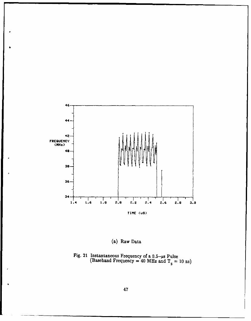
Fig. 21 Instantaneous Frequency of a 0.5-ps Pulse(Baseband Frequency = 40 MHz and Ts = 10 ns)

47

46-

44-

FREQUENCY(MHz)

40-

38-

36-

34 1

.4 1.6 1.8 2.8 2.2 2.4 2.6 2.8 3.0

TIME (uS)

(b) After Compensation

Fig. 21 Instantaneous Frequency of a 0.5---s Pulse(Baseband Frequency = 40 MHz and Ts = 10 ns)

48

46

44-

42

FREQUENCY(MHz)

46-

38

36-

34 -- - 7

1.4 1.6 1.8 2.8 2.2 2.4 2.6 2.8 3.8

TIME (uS)

(c) After Compensation and 3-point Moving Average

Fig. 21 Instantaneous Frequency of a 0.5--is Pulse(Baseband Frequency = 40 MHz and Ts = 10 ns)

49

applied to the noise, the resultant noise RMS value is found to decrease as expected. Whenthe moving average is increased from one sample to five contiguous samples, the RMSvalue of the noise is found to decrease by a factor of z (5)1/12. On the other hand, the signalpower is relatively unaffected. As a result, the output SNR improves as the number ofsamples used in the moving average is increased. This ha ppens because when a movingaverage is applied, the effective video bandwidth of the I/Q network is reduced byapproximately the square root of the number of samples used in the moving average. Aslong as the video bandwidth is larger than the video bandwidth of the signal, the measuredenvelope of the signal is not affected.

Figure 21 shows the instantaneous frequency distribution. The raw data shows thata peak-to-peak frequency deviation is about 4 MHz. When a 3-point moving average isused after compensation, the RMS instantaneous frequency error is reduced drastically tobelow 80 KHz. Other types of low-pass digital filters such as Butterworth and Chebyshevare also used on the compensated instantaneous frequency of the signal. However, they arefound to introduce ringing and overshoot which significantly distort the instantaneousfrequency.

7.3.2 Linear FM Signal

A linear FM signal with a center frequency of 1960 MHz, and a frequency excursionof 10 MHz is applied to the I/Q network. The envelope and instantaneous frequency areshown in Figs. 22 and 23 respectively. It has the same pulse width and input SNR as forthe pulsed signal. Even though the FM signal has a frequency excursion of 10 MHz, thesame set of compensation parameters are used as if it were a CW signal centered at 1960MHz. As can be seen from the plots, the compensated envelope and instantaneousfrequency of the input signal have been reproduced accurately. In other words, theimbalance errors and DC offsets of the I/Q network are relatively insensitive to frequencyvariations. As a result, coarser frequency calibration steps can be used.

8.0 SUMMARY AND CONCLUSIONS

A simple in-phase/quadrature (I/Q) demodulator architecture which can measurethe amplitude, phase and instantaneous frequency of radar signals has been examined inthis report. By splitting the in-phase and quadrature components of the input signal usinganalog components, this architecture is potentially useful for radar ESM applications wherewide instantaneous bandwidth and simple algorithms for extracting the modulationcharacteristics of radar signals are required. However, there are amplitude and phaseimbalance errors and DC offsets in practical I/Q networks, which can introduce largesystematic errors to the measurement. Two techniques, compensation and low-passfiltering using a moving average, have been proposed in this report for improving thissimple architecture.

The effect of amplitude and phase imbalances and DC offsets is found to produceripples on the measurement; the frequency of the ripples is harmonically related to thebaseband frequency of the signal. For a given set of imbalance errors and DC offsets, theerror introduced by the ripples on the instantaneous frequency is more severe and isdirectly proportional to the baseband frequency while the error is constant for both theamplitude and phase.

50

-1e

POWER(dBm)

-30-

-46-

1.4 1.6 1.8 2.6 2.2 2.4 2.6 2.8 3.8

TIME (uS)

(a) Raw Data

Fig. 22 Envelope of a Linear FM Pulse(Pulse Width = 0.5 ps, Center Frequency = 40 MHz,

Af = 10 MHz and Ts = 10 ns)

51

-29-

POMER(dBo)

-36-

-40-

1.4 1.6 1.8 2.8 2.2 2.4 2.6 2.8 3.8

TIME (uS)

(b) After Compensation and 5-point Moving Average

Fig. 22 Envelope of a Linear FM Pulse(Pulse Width = 0.5 ps, Center Frequency = 40 MHz,

af = 10 MHz and T. = I0 ns)

52

d1

4-

36 -Ii

(11=1Hzzan)T 1

353

3o -- -- I-I- TIL1.4 1.6 1.8 2.6 2.2 2.4 2.6 2.8 3.6

TIME (uS)

(a) Raw Data

Fig. 23 Instantaneous Frequency of a Linear FM Pulse( Pulse Width = 0.5 ps, Center Frequency = 40 MHz,

=f- 10 MHz and T8 -- 10 us)

53

45-

FREQUEMCY -(MHz)

40-

35-

as ' I r I r I

1.4 1.6 1.8 2.0 2.2 2.4 2.6 2.8 3.8

TINE (uS)

(b) After Compensation and 5-point Moving Average

Fig. 23 Instantaneous Frequency of a Linear FM Pulse(Pulse Width Up 0.5 ss, Center Frequency = 40 MHz,

af =10 MHz and Ts = 10 ns)

54

Some I/Q networks have been evaluated and the mean imbalance errors and DCoffsets over a large frequency range can be large. In order to keep the systematic errorssmall, some form of compensation is needed to remove the mean errors and offsets. Oncethe mean errors and offsets are eliminated, the residual RMS errors as a function offrequency and input power level are quite small. If further improvement is required, acalibration dependent on frequency and input power level may be needed.

The measurement accuracy on the amplitude, phase and instantaneous frequencyhas also been analyzed and given in terms of input SNR. For large inpu* SNR, the standarddeviation of the phase error decreases inversely proportional to the square root of the inputSNR while the standard deviation of the envelope remains constant as the input signallevel is varied.

There are two basic functions performed by using a moving average. The effectivenoise bandwidth of the I/Q network can be reduced with no appreciable degradations tothe signal of interest, with consequent improvement of the output SNR. The ripplesproduced by the imbalance errors and DC offsets are usually outside the video bandwidthof the signal of interest and thus can be reduced by low-pass filtering. In addition, amoving average is easy to implement digitally and does not introduce distortions such asringing and overshoot.

Both the techniques of compensation and low-pass filtering using a moving averagehave been successfully demonstrated on the demodulation of pulsed and linear FM signals.They have been shown to be effective for improving the output signal-to-noise ratio andreducing systematic errors.

55

9.0 REFERENCES

[1] J.B.Y. Tsui, Digital Microwave Receivers, Artech House Inc., Norwood, MA, 1989.

[2] D.L. Sharpin, J.B.Y. Tsui , and J. Hedge, " The Effects of Quadrature SamplingImbalances on a Phase Difference Analysis Technique "t, Proceedings of the IEEE,National Aerospace and Electronics Conference, NAECON 1990, Vols. 1-3;pp. 962-968, New York.

[3] S.J. Goldman, "1 Understanding the Limits of Quadrature Detection ", Microwave &RF, Dec, 1986.

[4] J.P.Y. Lee, " I/Q Demodulation: Time-domain Analysis on Systematic Errors'"to be published.

[5] E. Oran Brigham, The Fast Fourier Transform, Prentice-Hall, Inc. EnglewoodCliffs, New Jersey, 1974.

[61 A. Papoulis, Probability, Random Variables, and Stochastic Processes, McGraw-HillInc.,1965.

[7] A.V. Oppenheim and R.W. Schafer, Discrete-time Signal Processing, Prentice Hall,Englewood Cliffs, New Jersey, 1989.

[8] W.J. Lucas, " Tangential Sensitivity of a Detector Video System with R.F.Pre-amplification i", Proc. IEE, Vol. 113, No.8, pp. 1321-1330, August 1966.

[9] D. E. Johnson, Introduction to Filter Theory, Prentice-Hall, Inc. EnglewoodCliffs, New Jersey, 1976.

[10] H. Taub and D.L. Schilling, Principles of Communication Systems, McGraw-HillBook Company, 1971.

56

UNCLASSIFIED -57-SECURITY CLASSIFICATION OF FORM

(highest classification of Title. Abstract. Keywords)

DOCUMENT CONTROL DATA(Security classification of title, body of abstract end indexing annotation must be entered when the overall document is classified)

1. ORIGINATOR (the name and address of the organization preparing the document. 2. SECURITY CLASSIFICATIONOrganizations for whom the document was prepared, e.g. Establishment sponsoring (overall security classification of the documenta contractor's report, or tasking agency, are entered in section 8.) including special warning terms if applicable)NATIONAL DEFENCEDEFENCE RESEARCH ESTABLISHMENT OTTAWA UNCLASSIFIEDSHIRLEY BAY, OTTAWA, ONTARIO KIA 0K2 CANADA

3. TITLE (the complete document title as indicated on the title page. Its classification should be indicated by the appropriateabbreviation (SC or U) in parentheses after the title.)

I/Q DEMODULATION OF RADAR SIGNALS WITH CALIBRATION AND FILTERIZNG (U)

4. AUTHORS (Last name, first name, middle initial)

LEE, JIM P.

5. DATE OF PUBLICATION (month and year of publication of 6a NO. OF PAGES (total 6b. NO. OF REFS (totai cited indocument) containing information. Include document)

DECEMBER 1991 Annexes. Appendices. etc.)640

7. DESCRIPTIVE NOTES (the category of the document. e.g. technical report, technical note or memorandum. If appropriate, enter the type ofreport, e.g. interim, progress, summary, annual or final. Give the inclusive dates when a specific reporting period is covered.)

DREO REPORT

8. SPONSORING ACTIVITY (the name of the department project office or Laboratory sponsoring the research and development Include theNAdrsAL DEFENCE

DEFENCE RESEARCH ESTABLISHMENT OTTAWASHIRLEY BAY, OTTAWA, ONTARIO KIA 0K2 CANADA

9a. PROJECT OR GRANT NO. (if appropriate, the applicable research 9b. CONTRACT NO. (if appropriate, the applicable number underand development project or grant number under which the document which the document was writteniwas written. Please specify whether prolect or grant)

011LBI110a. ORIGINATOR'S DOCUMENT NUMBER (the official document 10b. OTHER DOCUMENT NOS. (Any other numbers which may

number by which the document is identified by the originating be assigned this document either by the originator or by theactivity. This number must be unique to this document) sponsor)

DREO REPORT 1119

1 1. DOCUMENT AVAILABILITY (any limitations on further dissemination of the document. other than those imposed by security classification)

(lXJ Unlimited distributionI ) Distribution limited to defence departments and defence contractors; further distribution only as approved

D Distribution limited to defence departments and Canadian defence contractors; further distribution only as approved

D ) Distribution limited to government departments and agencies; further distribution only as approved

D I Distribution limited to defence departments; further distribution only as approved

( ) Other (please specify):

12. DOCUMENT ANNOUNCEMENT (any limitation to the bibliographic announcement of this document This will normally correspond tothe Document Availabilty (11). However, where further distribution (beyono the audience specified in 11) is possible, a widerannouncement audience may be selected.)

UNCLASSIFIED

SECURITY CLASSIFICATION OF FORMOCD03 2/06/87

-58- UNCLASSIFIED

SECURITY CLASSIFICATION OF FORM

13. ABSTRACT ( a brief and factual summary of the document It may also appear elsewhere in the body of the document itself. It is highlydesirable that the abstract of classified documents be unclassified, Each paragraph of the abstract shall begin with an indication of thesecurity classification of the information in the paragraph (unless the document itself is unclassified) represented as (S), (). or (Ui.It is not necessary to include here abstracts in both offical languages unless the text is bilingual).

(U) A simple in-phase/quadrature (I/Q) demodulator architecture which canmeasure the amplitude, phase and instantaneous frequency of radar signals is examinedin this report. This architecture has a potential for radar ESM applications wherewide instantaneous bandwidth and simple algorithms for extracting the modulationcharacteristics of radar signals are required. This I/Q architecture can meet therequirement by splitting an incoming signal into its in-phase and quadraturecomponents using analog circuitries. However in practice, there are amplitude andphase imbalances between the two components and DC offsets, which can introduce largesystematic errors to the measurement. In this report, we present novel techniqueswhich can greatly reduce the systematic errors and improve the accuracy of themeasurement. A time-domain analysis on the systematic errors is given. A calibrationtechnique which can be used to correct for the imbalances and offsets is discussed.The effect of noise on the accuracy of the measurement is also examined. Imbalanceerrors and DC offsets of I/Q networks are measured and analyzed. Finally, a post-processing technique employing moving averages, which is shown to be effective forimproving the output signal-to-noise ratio and reducing systematic errors, is alsopresented.

14. KEYWORDS. DESCRIPTORS or IDENTIFIERS (technically meaningful terms or short phrases that characterize a document and could behelpful in cataloguing the document They should be selected so that no security classification is required. Identifiers, such as equipmentmodel designation, trade name. military prolect code name. geographic location may also be included. If possible keywords should be selectedfrom a published thesaurus. e.g. Thesaurus of Engineering and Scientific Terms (TEST) and that thesaurus-identified. If it is not possible toselect indexing terms which are Unclassified, the classification of each should be indicated as with the title.)

I/ Q DEMODUALTIONRADAR ESMDIGITAL RECEIVERRADAR SIGNAL PARAMETER MEASUREMENT

UNCLASSIFIED

SECURITY CLASSIFICATION OF FORM