hyperspectral image analysis - pci geomatics · · 2015-04-28hyperspectral image analysis 1....

Hyperspectral Image Analysis

Hyperspectral Image Analysis Geomatica 9 Version 9.1

Copyright Notice This publication is a copyrighted work owned by: PCI Geomatics 50 West Wilmot Street Richmond Hill, Ontario Canada L4B 1M5 www.pcigeomatics.com The information in this document is subject to change without notice and should not be construed as a commitment by PCI Geomatics. PCI Geomatics assumes no responsibility for any errors that may appear in this document. The software described in this document is furnished under a license and may only be used or copied in accordance with the terms of such license. No responsibility is assumed for the use or reliability of the information that is derived through the use of PCI Geomatics software. Copyright © 1996-2004 by PCI Geomatics. All rights reserved. All copies must contain this notice in its entirety.

Trademark Acknowledgements Geomatica, EASI/PACE, ImageWorks, GCPWorks, OrthoEngine, GeoGateway, RADARSOFT, FLY!, PCI Author, PCI Modeler, GeoAnalyst, and Agroma are registered trademarks of PCI Geomatics. InstallShield is a registered trademark of InstallShield Software Corporation. Microsoft is a registered trademark, and Windows is a trademark of Microsoft Corporation. MrSID is a registered trademark of LIZARDTECH Inc. Copyright 1995-2004. All rights reserved. UNIX is a registered trademark of UNIX System Laboratories Inc. All other trademarks and registered trademarks are the properties of their reserved owners.

Questions? [email protected] 1


Table of Contents 1. Introduction 3 2. Background 3 3. Spectral Libraries 4 4. Data Preparation 5 4.1 Metadata 5 4.2 Preprocessing Algorithms 5 4.3 Noise Removal 6 5. Data Visualization 8 5.1 3D Data Cube 8 5.2 Thumbnails 8 5.3 Band Cycling Tool 9 6. Data Compression 9 7. Atmospheric Correction 10 7.1 Radiance and Reflectance 10 7.2 Simple Atmospheric Correction 10 7.3 Model-based Atmospheric Transformation 11 7.4 Future Enhancements 11 8. Image Analysis 12 8.1 Endmember Selection 12 8.2 Spectral Linear Unmixing 12 8.3 Spectral Angle Mapper 13 9. Summary 13



1. Introduction Recent advances in remote sensing and developments in hyperspectral sensors have allowed these types of data to be used by people other than spectral remote sensing experts. Not only has the technology for acquiring these types of data been improved, but advances have also been made in analysis techniques. Hyperspectral data were once restricted mainly to geological applications. Today however, the range of disciplines that can use this information has grown to include ecology, atmospheric science, agriculture and forestry to name just a few. Because hyperspectral remote sensing, also known as imaging spectroscopy, provides more detailed information than mutlispectral imaging, we are able to identify and differentiate spectrally unique materials. This paper will explore some of the differences between hyperspectral and multispectral remote sensing, discuss preprocessing techniques, data visualization, data compression, atmospheric correction and image analysis.

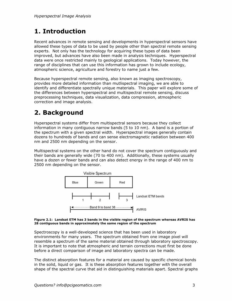
2. Background Hyperspectral systems differ from multispectral sensors because they collect information in many contiguous narrow bands (5 to 10 nm). A band is a portion of the spectrum with a given spectral width. Hyperspectral images generally contain dozens to hundreds of bands and can sense electromagnetic radiation between 400 nm and 2500 nm depending on the sensor. Multispectral systems on the other hand do not cover the spectrum contiguously and their bands are generally wide (70 to 400 nm). Additionally, these systems usually have a dozen or fewer bands and can also detect energy in the range of 400 nm to 2500 nm depending on the sensor.

Figure 2.1: Landsat ETM has 3 bands in the visible region of the spectrum whereas AVRIS has 28 contiguous bands in approximately the same region of the spectrum Spectroscopy is a well-developed science that has been used in laboratory environments for many years. The spectrum obtained from one image pixel will resemble a spectrum of the same material obtained through laboratory spectroscopy. It is important to note that atmospheric and terrain corrections must first be done before a direct comparison of image and laboratory spectra can be made. The distinct absorption features for a material are caused by specific chemical bonds in the solid, liquid or gas. It is these absorption features together with the overall shape of the spectral curve that aid in distinguishing materials apart. Spectral graphs



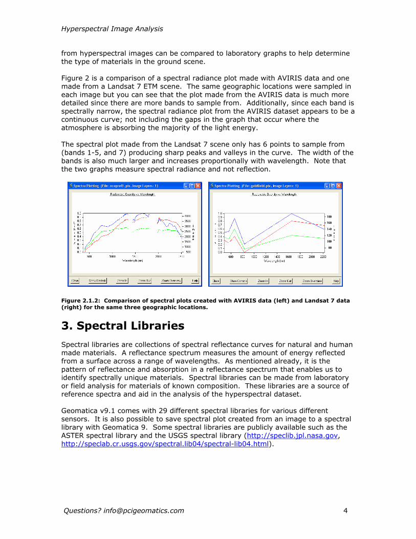
from hyperspectral images can be compared to laboratory graphs to help determine the type of materials in the ground scene. Figure 2 is a comparison of a spectral radiance plot made with AVIRIS data and one made from a Landsat 7 ETM scene. The same geographic locations were sampled in each image but you can see that the plot made from the AVIRIS data is much more detailed since there are more bands to sample from. Additionally, since each band is spectrally narrow, the spectral radiance plot from the AVIRIS dataset appears to be a continuous curve; not including the gaps in the graph that occur where the atmosphere is absorbing the majority of the light energy. The spectral plot made from the Landsat 7 scene only has 6 points to sample from (bands 1-5, and 7) producing sharp peaks and valleys in the curve. The width of the bands is also much larger and increases proportionally with wavelength. Note that the two graphs measure spectral radiance and not reflection. Figure 2.1.2: Comparison of spectral plots created with AVIRIS data (left) and Landsat 7 data (right) for the same three geographic locations.

3. Spectral Libraries Spectral libraries are collections of spectral reflectance curves for natural and human made materials. A reflectance spectrum measures the amount of energy reflected from a surface across a range of wavelengths. As mentioned already, it is the pattern of reflectance and absorption in a reflectance spectrum that enables us to identify spectrally unique materials. Spectral libraries can be made from laboratory or field analysis for materials of known composition. These libraries are a source of reference spectra and aid in the analysis of the hyperspectral dataset. Geomatica v9.1 comes with 29 different spectral libraries for various different sensors. It is also possible to save spectral plot created from an image to a spectral library with Geomatica 9. Some spectral libraries are publicly available such as the ASTER spectral library and the USGS spectral library (http://speclib.jpl.nasa.gov, http://speclab.cr.usgs.gov/spectral.lib04/spectral-lib04.html).


http://speclib.jpl.nasa.gov/

http://speclab.cr.usgs.gov/spectral.lib04/spectral-lib04.html


Figure 3.1: Reference reflectance spectra can be plotted in Geomatica using the Spectra Plotting tool. Actinolite, dolomite, and kaolinite were plotted using information contained in a spectral library.

4. Data Preparation

4.1 Metadata Entering the metadata into xml format is the first step in preparing your hyperspectral data set to be used in Geomatica 9. Most hyperspectral data sets come with additional information about the mission and the sensor used to acquire the data. There are two categories for the metadata items to be entered; the Global Metadata items apply to the sensor or image as a whole and the Band Specific Metadata items apply only to the band as the name suggests. Importing meta-data is important when working with hyperspectral data since many of the programs and tools in the advanced hyperspectral package make extensive use of this information. For example, when creating a spectral plot for a ground feature in an image, it is the metadata item describing the bands response profile that allows the wavelength to be displayed along the x-axis of the graph.

4.2 Preprocessing Algorithms Imagery obtained with airborne hyperspectral systems that use pushbroom scanners often produce imagery that appears wavy. This can be caused by aircraft roll during data acquisition. Polynomial correction, a statistical rectifier, is not suited for correcting this type of distortion since it is non-systematic. Therefore, this wavy deformation must be corrected before geocorrecting the data.



Figure 4.2.1: Distortion caused by aircraft roll is apparent in the upper portion of this image

The ROLLCOR algorithm within Geomatica was specifically designed to correct this type of distortion in hyperspectral imagery. Starting with the second image scanline, ROLLCOR shifts each scanline relative to the previous one by an integer number of pixel positions to either the left or right. Some additional algorithms available within Geomatica for preprocessing the data include: BRDFCOR – Cross-swath Brightness Correction, and STRPCOR – Stripe Correction. These programs would also be used before performing any analysis on the dataset. Hyperspectral images are geocorrected using the same techniques employed for greyscale or multispectral imagery by collecting GCPs. NASAs spaceborne hyperspectral imager, Hyperion, is supported in Geomatica OrthoEngine’s generic satellite model. There is no limit to the number of bands in an image that can be geocorrected in OrthoEngine.

4.3 Noise Removal Most hyperspectral datasets are able to collect a continuous spectrum of energy in the range of 400 to 2500 nm. This large amount of information provides a great deal of detail but also increases the processing time during analysis. Since by definition the bands in hyperspectral datasets are spectrally narrow, the information that they contain is often redundant. Additionally, some bands are affected by noise or atmospheric absorption rendering them unusable for analysis.



Figure 4.3.1: The Thumbnails visualization tool was used to show that bands 108 – 112 are all affected by noise. The top left image displayed is band 106 increasing from left to right to band 114. Maximum Noise Fraction Linear Transformation (MNFLT) and Principal Components Linear Transformation (PCLT) both reduce the dimensionality of a data set in conjunction with the Linear Transformation algorithm (LINTRN). MNFLT produces component images that are ordered in terms of image quality. This method seeks to concentrate image noise present in the input channels into as few output components as possible. In contrast, PCLT seeks to concentrate image variance into as few output components as possible. The workflow for MNFLT and PCLT is similar. Either MNFLT or PCLT is used to linearly transform the channels affected by noise in the dataset. Then LINTRN (Linear Transformation) uses the parameters of the linear transformation from MNFLT or PCLT to generate the forward transformed bands. An average filter is then applied to the forward transformed bands. The inverse of the MNFLT or PCLT transformation is then applied to the altered forward transformation results. Finally, these inverse transformation results are used to replace the original noisy bands. Maximum Noise Fraction Base Noise Removal is another way of removing bands affected by noise in a dataset. The program MNFNR could be used if in a set of image bands, one band is considered to have significantly more noise than the others, and it is desirable to transform that band such that its noise content is close to that of the other bands. In this case, it is not necessary to know the noise variance in any band in order to define the MNFNR transform.



5. Data Visualization Because of the large amount of data contained in a hyperspectral data set, visualization for these types of images is often difficult. PCI Geomatics has incorporated three tools to facilitate the visualization of these large datasets – the 3D Data Cube, the Thumbnails viewer and the Band Cycling tool.

5.1 3D Data Cube A common method for displaying hyperspectral imagery is a 3-D data cube. The X-Y plane holds the spatial information and the Z-axis represents the spectral information in the file. The 3D Data cube helps you to get a sense for the structure of the data you are working with by letting you assess the number and nature of spectra endmembers present in the scene. It is useful to see the spectral bands where there is high atmospheric absorption and thus very little signal reaching the sensor - black layers. The 3D data cube is available through Geomatica Focus. This tools allows a user to display, rotate, and excavate the data in three-dimensions. This excavation is useful in visualizing how the spectral response for ground features changes with wavelength.

Figure 5.1.1: 3D Data Cube

5.2 Thumbnails The thumbnails tool in Geomatica Focus is another effective way to visualize a raster dataset with many channels. The thumbnails tool allows you to display all or a selection of the bands in a hyperspectral dataset simultaneously. Bands that are severely affected by noise or atmospheric effects can be easily discriminated. This is also a useful tool in selecting bands to display in either greyscale or as colour composites in the Focus viewer.



Figure 5.2.1: Thumbnails Viewer

5.3 Band Cycling Tool Band cycling is a quick way to cycle through different channel or wavelength ranges in a specified color component, to create new color composites. This tool allows a user to observe the progressive change that increasing or decreasing the band number being displayed in one of the colour display layers has on the composite. Rapid change in appearance over particular wavelength regions may be diagnostic of certain material

er

6. Data Compression It is the large amount of information in a hyperspectral dataset that enables us to distinguish and identify spectrally unique materials in an image. However, the size of hyperspectral imagery means that they occupy a great deal of memory and render computations slower compared to multispectral datasets. A compression technique called vector quantization designed specifically for hyperspectral imagery is available in PCI Geomatics. It transforms a multiband image using the Hierarchical Self-Organizing Cluster Vector Quantization algorithm. This saves in storage space and reduces the program execution time for large images. Since the algorithms in the Advanced Hyperspectral package in Geomatica 9 can read vector quantized image data generated with the VQHSOC algorithm, initial tests can be performed with the compressed data to determine the parameters to be used for a given program. Once the optimal parameters have been determined, the final test can be done with the original uncompressed data.



7. Atmospheric Correction

7.1 Radiance and Reflectance It is important to make the distinction between radiance and reflectance before using spectral libraries to analyze remotely sensed data. Sensor radiance measures the amount of light energy reaching a sensor. Reflectance on the other hand is the percentage of light incident on a surface that is then reflected by that material. Light that is not reflected is absorbed or transmitted by the surface. Surface reflectance is only one factor that influences spectral radiance. Some of the other factors affecting sensor radiance include terrain features, interactions with the atmosphere and the spectrum of incoming radiation. Because of gaseous and liquid particles in the earth’s atmosphere, radiance seldom equals reflectance. Therefore atmospheric correction must be done to be able to compare the spectral plot from an image to that obtained through lab spectroscopy. For flat terrain that is uniformly irradiated by the sun, a scene radiance map differs from a reflectance map by only a constant factor. Radiance values must be converted to reflectance values before comparing image spectra with reference reflectance spectra. This can be done using either simple atmospheric correction or model based atmospheric correction.

7.2 Simple Atmospheric Correction FTLOC is an image-based correction method that locates spectrally flat targets in the image. The “flat” image-derived spectra that are located with FTLOC can be used to create a radiometric transformation that reduces the presence of atmospheric absorption features in the image data. Solar irradiance as well as atmospheric scattering and absorption can be assumed to contribute the most to the mean spectrum of these flat areas. Therefore, dividing each spectrum in the image by the mean of the flat spectrum converts a scene to relative reflectance. The transformed image is more suitable for comparison with ground or laboratory measured reflectance spectra than is the original image. An empirical line calibration (EMPLINE) converts an image to apparent reflectance values. A reference reflectance spectrum (typically acquired on the ground) is required for each of one or more targets that appear in the image data. In the case of two or more input reflectance spectra, the resulting transformation for each band is computed by regressing the band reflectance values for all of the regions of interest (ROIs) on the image values for all of the ROIs. The slope of the regression line (see figure 8) equals the gain to be stored for the image band; the intercept of the regression line equals the offset to be stored for the image band.



Figure 7.1.1: Regression line formed by plotting the radiance against reflectance for two ROIs representing the same ground feature.

7.3 Model-based Atmospheric Transformation Model-based atmospheric transformation consists of either the transformation of an at-sensor radiance dataset to a reflectance dataset, or the transformation of a reflectance dataset to an at-sensor radiance dataset. When starting with a radiance dataset, this provides a more rigorous alternative to the techniques described by Simple Atmospheric Correction for atmospheric correction. Model-based implies a transformation technique that involves a model of the interaction of light with the atmosphere (i.e., radiative transfer), the imaging situation, and the sensor. The specific technique that is implemented in Geomatica 9 is based on the technique implemented in the Canada Centre for Remote Sensing Imaging (CCRS) Spectrometer Data Analysis System (ISDAS). Atmospheric transformation using an at-sensor radiance look up table (ATRLUT) converts an input radiance dataset into a reflectance dataset, or converts an input reflectance dataset into a radiance dataset. The computations use radiance values interpolated from an at-sensor radiance look-up table (RLUT). The RLUT is created with the programs GENTP5, GENRLUT included in the Geomatica 9 Advanced Hyperspectral package and the Modtran4 program.

7.4 Future Enhancements PCI Geomatics is currently developing the following enhancements to the atmospheric transformation technique:

•

•

•

•

An extension to ATRLUT that will allow it to take into account adjacency radiance effects due to heterogeneous scene reflectance.

The addition of a program for estimating the vertical water vapour content value on a pixel-by-pixel basis from the radiance dataset and RLUT.

An extension to ATRLUT that will allow pixel-by-pixel elevation and vertical water vapour content values to be read from raster maps.

The addition of a program for detecting spectral line curvature in a radiance dataset and generating a correction look-up table for the dataset.



• An extension to ATRLUT that will allow it to apply a spectral line curvature

correction look-up table to a radiance dataset when applying a radiance-to-reflectance transformation.

8. Image Analysis Unique image analysis algorithms have been developed for hyperspectral imagery to take advantage of the large amount of information they contain. Most of these algorithms are designed to determine the materials that make up the ground features in the image. Some of the main image analysis algorithms included in the Geomatica Advanced Hyperspectral package are ENDMEMB (Endmember Selection), SPUNMIX (Spectral Linear Unmixing) and SAM (Spectral Angle Mapper).

8.1 Endmember Selection ENDMEMB is used to compute a set of endmember spectra using the image as input. This is the first step for the spectral linear unmixing process. Endmembers can be thought of as classes or a set of spectra that make up a hyperspectral image. When these endmembers are linearly combined, they should ideally form all the observed spectra in an image.

8.2 Spectral Linear Unmixing SPUNMIX linearly unmixes a hyperspectral image using a set of endmember spectra. SPUNMIX evaluates a fraction-map for each spectrum in the set. The resulting pixel values in the fraction-map are estimates of the fractional contribution of each endmember spectrum to the corresponding pixel’s band vector (i.e., the “endmember fractions” for a pixel) for the hyperspectral dataset. Spectral unmixing can be used to determine information on a “subpixel” scale. It is a method ideally suited to extracting information from “mixed pixels”, and therefore has many applications in geology, ecology, and hydrology. Whereas traditional image classifiers are used to classify each image pixel into one of a number of classes, spectral unmixing is used to assign fractional class membership to each image pixel. Therefore, rather than producing one classification image, spectral unmixing produces one raster map per class, where the map values indicate the fraction of the pixel assigned to the class. Spectral unmixing thus makes sense when one has an image composed of mixed pixels, from which one wishes to determine the endmember fractions. Spectral unmixing is particularly valuable when the image data are of low spatial resolution with respect to the scene cover types of interest. This is often the case with hyperspectral images. The concept of spectral unmixing makes sense if you are working with pixels that are generally larger then the size of the occurrence of endmembers of interest, and hence most of the pixels are “mixed pixels”. In that case, the question is not “Which endmember is associated with this pixel?”, but rather “What endmembers contribute to this pixel, and what is the relative contribution of each; what are the endmember fractions?”.




8.3 Spectral Angle Mapper The Spectral Angle Mapper (SAM) is designed to classify hyperspectral image data, on the basis of a set of reference spectra that define the classes. SAM computes the "spectral angle" between each band vector in a specified region of the input raster layers and each of the reference spectra read from the input spectra file (Spectral Library) (the spectra are treated as band vectors for the purpose of the angle computation). The smaller the angle, the more similar the pixel is to the band vector, or target. The result is a raster layer that indicates for each image pixel the input reference spectrum with which it has the smallest angle (the minimum spectral angle). The results from SAM are unaffected by the relative scaling of the image band vectors and the reference spectra. This is because the angle between two vectors depends only on the directions of the vectors and not on their magnitudes. Therefore, if the image data differs from the physical units of the reference spectra by only a "gain" factor that is uniform over all bands, then the SAM results will be exactly the same as if the image data were perfectly calibrated to the spectra units. Note that this is generally not the case if the reference spectra represent material reflectance and the image data represent at-sensor radiance. Spectral angle classification is most useful when the image is mostly comprised of pixels that correspond to terrain elements consisting of a single, spectrally distinct material class of interest (i.e., when the pixels are "pure").

Figure 8.3.1: A two-dimensional illustration of a spectral angle map. In reality the calculation would be based on more than two bands creating a “hyper-angle” between the image pixel values and the reference spectra

9. Summary Hyperspectral data provide much more information compared with multispectral data. Because of the large size that these datasets can reach, new visualization, compression, and analysis techniques have been developed. The Advanced Hyperspectral package in Geomatica 9 provides users with viewing and analytical tools, and the ability to reduce the amount of time needed to process hyperspectral data through the Canadian Space Agency’s Vector Quantization compression technique. These new capabilities provide users with the capability to better analyze and view hyperspectral data and make it easier to integrate it with other geospatial data.

hyperspectral image analysis - pci geomatics · · 2015-04-28hyperspectral image analysis 1....

Documents