hydrodynamics and eutrophication model study of indian

Technical Report EL-94-5May 19

AD-A282 922US Army Corpsof EngineersWaterways ExperimentStation

Hydrodynamics and EutrophicationModel Study of Indian River andRehoboth Bay, Delaware

by Carl F. Cerco, Barry Bunch,Mary A. Cialone, Harry Wang

DTICS

ELECTES AUG 0 2 1994- -

Approved For Public Release; Distribution Is Unlimited

94-242574$94 8 01 031

Prepared for U.S. Environmental Protection AgencyDelaware Department of Natural Resources and Environmental Control

and U.S. Army Engineer District, Philadelphia

The contents of this report are not to be used for advertising,publication, or promotional purposes. Citation of trade namesdoes not constitute an official endorsement or approval ofthe useof such commercial products.

0 IqWPmm ON 3M PAmiR

Technical Report EL-94-5May 1994

Hydrodynamics and EutrophicationModel Study of Indian River andRehoboth Bay, Delawareby Carl F. Cerco, Barry Bunch,

Mary A. Cialone, Harry Wang Accesion For

U.S. Army Corps of Engineers NTIS CRA&IWaterways Experiment Station DTIC TAB3909 Halls Ferry Road Unannounced 0Vicksburg, MS 39180-6199 Justification

By ........

DisA d ibution I

Availability Codes

Avail and/or aDist Special

Final Report

Prepared for U.S. Environmental Protection Agency, Region IIIPhiladelphia, PA 19107

Delaware Department of Natural Resources and Environmental Control

Dover, DE 19903

and U.S. Army Engineer District, PhiladelphiaPhiladelphia, PA 19106-2991

US Army Corps

Waterways Experiment SainCtlgn~nPblalnDtStydrodyaisanetohcto oe td fIda ie n

District, Philadlph9a

1.rwy Eutrph dtcSation - eaarel-eoboth Bay 2. HydodnDatesMathematial d moes. .Cercaon Cadel F. of. UItediSates.vArmy ConsdEnines PBayDelahiar DistCril FI. Uned St.atesl.) Environentale PoroUec-

EvrnetlPoetion Agency. Region Ill.,V Delaware. Depa.o aua eormest andNtrlRsucsadEnvironmental Control. V.d U.S. Armry Engineer WtrasEprmn

Statio. :VM. Se;s 21 m Technical report (US;Am Engner4at-wyExperiment Sation)- ;elar E9--RhbohSy.2

MaTA7 ca modls 1.no.ELa F I.Uitd tte.Arn opso

Contents

P eface ..... .......................................... v

I-Introduction ....................................... 1-1

The Study System ..................................... 1-1Objectives .......................................... 1-1

&1-Data Bases ......................................... 2-1

Hydrograpic Data Bases ................................ 2-1Woawe Quality Data .................................... 2-4

l .-Flows and ads .................................... 3-1

Flows ............................................. 3-1Loads ............................................. 3-7

IV-DescnPtm of the Hydrdynamic Model .................... 4-1

Governing Equaions ................................... .4-1Non-Dimensionalization of Governing Equations ............... 4-5Trunsfomation of Governing Equations ................... 4-6Finite Difference Aproximations of

Governingo quadons .................................. 4-9

V-Hydrodynamic Model Application ......................... 5-1

Numerical Oid Developme .......................... S-IModel Calibration and Valdation ....................... 5-3Calibration Overview ................................... 5-3Calbration Cnditions .................................. 5-5Calibration Pocedue .................................. 5-5Analysis of Calibraon• Raesults ............................ 5-6Validation Conditions .................................. 5-11Analysis of Valtion Results ............................ 5-18Salizf Overview ................................ 5-18Slind t Calibration and Validation ......................... 5-28Summner Aveuge Salnity ................................ 5-33

Vl--Wmr Quality Model Kinetics ........................... 6-1

Ud ction ......................................... 6-1Coaervatia of Mass Equati ......................... 6-3

In

A lgae .............................................. 6-4Organic Carbon ....................................... 6-18Phosphorus .......................................... 6-23Nitrogen . 6-28Dissolved Oxygen ..................................... 6-35Salinity ............................................ 6-37Temperature ......................................... 6-37Summary of Kinetics Coefficients .......................... 6-38

VI-Linking the Hydrodynamic and Water Quality Models .......... 7-1

Intloduction ........................................... 7-1Water Quality Model Time Step ........................... 7-2Linkag Testing .................................... 7-4

VIII-Additional Model Inputs and Outputs ..................... 8-1

Introduction ......................................... 8-iPatiion of Loads ..................................... 8-1Open-Mouth Boundary Condition ......................... 8-3Light Fm ton ...................................... 8-4Sediment-Water Fluxes ................................. 8-8

mU t ion of BOD ................................... 8-16Diunad Dissolved Oxygen Fluctuatins ...................... 8-18

IX-War Quality Model Application and Analysis ............... 9-1

WSa r Quality Time Series ............................... 9-1L ngkit al T im- .................................. 9-1Sediiem-Wam . Fluxes ................................. 9-2Imerpretive Infomatim o............................... 9-2Evaluation of Model Performane•.......................... 9-52The Ammal Cycle of Water Quality ........................ 9-69Summer-Avemge Watr Quality ........................... 9-76

X--CamrlCUuiOs and Reco mngdat ........................ 10-

Conclusions ......................................... 10-Ilwcommedati,..................................... 10-2

References ........................................ Ref- I

SF298

Iv

Preface

The Hydrodynamic-Eutrophication Model Study of the Delaware InlandBays was sponsored by the U.S. Environmental Protection Agency, Region III(USEPA), the Delaware Department of Natural Resources and EnvironmentalControl (DNREC), and the U.S. Army Engineer District, Philadelphia(CENAP). Project monitors were Messrs. Charles App and Robert Runowski,USEPA, Mr. John Schneider, DNREC, and Mr. Jeff Gebert, CENAP.

The eutrophication modeling was conducted by Drs. Carl F. Cerco andBarry Bunch, Water Quality and Contaminant Modeling Branch (WQCMB),Environmental Laboratory (EL), U.S. Army Engineer Waterways ExperimentStation (WES). Supervision of the eutrophication model activities wasprovided by Dr. Mark Dortch, Chief, WQCMB.

The hydrodynamic modeling was conducted by Ms. Mary Cialone, CoastalProcesses Branch (CPB), and Dr. Harry Wang, Coastal Oceanography Branch(COB), Coastal Engineering Research Center (CERC), WES. Supervision ofthe hydrodynamic model activities was provided by Mr. Bruce Ebersole, Chief,CPB, and Dr. Martin Miller, Chief, COB.

Project management was provided by Mr. Donald Robey, Chief, Environ-mental Processes and Effects Division, EL, and Mr. H. Lee Butler, Chief,Research Division, CERC. Overall supervision was provided by Dr. JohnHarrison, Director, EL, and Dr. James Houston, Director, CERC.

At the time of publication of this report, WES Director was Dr. Robert W.

Whalin. Commander was COL Bruce K. Howard, EN.

This report should be cited as follows:

Cerco, C. F., Bunch, B., Cialone, M. A., and Wang, H.(1994). "Hydrodynamic and eutrophication model study ofIndian River and Rehoboth Bay, Delaware," TechnicalReport EL-94-5, U.S. Army Engineer Waterways ExperimentStation, Vicksburg, MS.

V

Chapter I: Introduction

The Study System

Indian River and Rehoboth Bay (Figure 1-1) are two water bodies that formpart of the interlocked Delawav Inland Bays system. Rehoboth Bay is con-nected to Delaware Bay to the north via a canal and to Indian River Bay to thesouth. Indian River Bay is connected to the Atlantic Ocean on the east via aninlet and to Little Assawoman Bay via a canal to the south. The westernportion of Indian River Bay, referred to as Indian River, terminates at theMillsboro dam. Drainage area of the system is 55647 hectares (Ritter 1986) ofwhich 14339 hectares is upstream of the impoundment at Millsboro. Thebasin contains one long-term stream gauging station (USGS 01484500) onStockley Branch. Mean flow for the period of record (43 years) is 0.196 m3

sec"1 or 1.44 x 10 -4 m3 sec"1 hectare- . Employing the runoff at Stockley tocharacterize the remainder of the basin indicates a long-term basin mean flowof 8.03 m3 sec"1.

Surface area and volume of the system are 7.31 x l0e m2 and 1.21 x 108m3 respectively. Mean depth is 1.66 m which characterizes most of the systemexcept near the inlet in which local mean depth exceeds ten meters. Mean tiderange at the inlet is 1.25 m (Smullen 1992). The tidal prism is 51 x 106 m 3

(Smullen 1992). The system is well-mixed from surface to bottom and issaline vinually throughout its extent. Median salinity is 22.7 ppt and 95% ofobservations exceed 4.3 ppt. Lowest salinities occur immediately downstreamof the Millsboro dam during periods of high runoff. Residence time of thesystem, determined as volume divided by freshwater flow rate is lengthy:174 days. An alternate estimate of residence time, volume divided by tidalprsm over the tidal period, is much less: 1.2 days. Except near headwatersand in constricted areas in which the tide is dampened, tidal flushing is moreeffective than runoff in the determination of volumetric flows and mass trans-port throughout the system.

Objectives

The primary objective of this study is to provide a hydrodynamic/waterquality model packge of the Indian River - Rehoboth Bay system. The

Chorw I 1-1n~

LewesATIANTIC

OCEAM

RehobothBeach

FGuorgetow.Inn RivrHndReBOthBa

IDA IVER

SBethany• Beach

Figure 1-1. Indian River and Rehoboth Bay

package is to be suitable for developmem of total maximum daily loads, point-source waste load allocations, and nonpoint-source load allocations of nutriesand organic substances. Additional requirements are that the model packageoperate in a continuous multi-year mode and provide information on diurnaldissolved oxygen variations. The model package is also to provide an orga-nized framework for collection and employment of additional observations inthe study system. The period covered by the study extends from January 1988to December 1990.

1-2 h. II ad.ci

Chapter I1: Data Bases

Hydrographic Data Bases

Bathymetry

A hydrographic survey of the dual bay and inlet system was performed in1988 by the U.S. Army Engineer District, Philadelphia. The survey was refer-enced to State Plane coordinates and all soundings were referenced to NationalGeographic Vertical Datum (NGVD). These data were used to determine thedepth in each cell of the Indian River-Rehoboth Bay grid by applying a3-point linear interpolation scheme to the data. In addition, the data were con-verted from State Plane coordinates to map inches for consistency between thegrid reference system and bathymetric reference system.

Tide gages

Tide data referenced to NGVD were collected by the United States Geo-logic Survey at five locations (Figure 2-1). These data (Table 2-I) were usedto specify the inlet boundary condition and for calibration purposes. Tiderecords at the inlet were not complete for the three-year model applicationperiod, 1988-1990. Missing data were obtained by transformation of tiderecords at Lewes, Delaware. The transformation was accomplished by com-paring the inlet and Lewes gages for the time period when data were availableat both gages and establishing a relationship between the two gages.

Current meftrs

Velocity data employed in the model calibration were collected at fourlocations near Middle Island from 30 June to I July 1988 (Figure 2-1 andTable 2-2).

ChWr 2 DMBM

Figue 21. Gugeloction fo moel cibrtio

Wind Dat

vidr -1Gued woaiond data atthmower palbatint Fgr ) ete aafo hoe

2-2 ~ in Dat2Dasemg

Table 2-1Tide Gauge Data

Location Gouge Number N"wthlng Easting Tinm Pewod

Vines 01484549 202070 560870 06-29-88 to 07-05-8810-01-88 to 09-30-89

(TI) 0--01-89 to 10--13-8907-06-90 to 09-30-90

Potnets 01484605 222270 576670 06-29-88 to 09-30-8810-01-88 to 09-07-89

(T2) 09-25-89 to 09-30-8910-01-89 to 07-17-90

Massey 01484680 227670 590800 06-29-88 to 08-15-8808-17-88 to 09-30-88

(T3) 10-01-88 to 09-30-8910-01-89 to 07-17--90

Dewey 01484670 253070 594750 06-29-88 to 07-05-8810-01-88 to 09-30-89

(T4) 10-31-89 to 09-30-9010-01--90 to 11-04-91

Inlet (USCG) 01484683 222170 599600 06-29-88 to 09-30 8810-01-88 to 10-09-88

(T5) 10-13-88 to 06-19-89

Table 2-2

Current Meter Data

Location Northing Easilng Tim Pa

east of Middle Island 224610 592800 06-30-88 to 07-01-88(east gauge) (CM1)

east of Middle Island 224900 592470 06-30-88 to 07-01-88(west gauge) (CM2)

west of Middle Island 225600 591330 06-30-88 to 07-01-88(east gauge) (CM3)

west of Middle Island 225730 591200 06-30-88 to 07-01-88(west gauge) (CM4) _ _I

Delaware Air Force Base provided the third source of wind data. For the 1988calibration, data from the DPL anemometer were used because this local datasource was most complete. For the 1989 and 1990 simulations, weather datafrom Dover was the most complete data source and was therefore utilized.

2-3Chpwr 2 OntoBaSem

Water Quality Data

STORET

Data from over 60 stations within the Indian River - Rehoboth Bay water-shed was retrieved from the STORET data base. Stations were plotted ontopographic maps according to reported longitude and latitude. In many cases,reported longitude and latitude were not consistent with landmarks in the sta-tion descriptions. Longitude and latitude were then revised to conform tostation descriptions. Some stations could not be accurately located and weredropped as were stations that contained no water quality constituents of inter-est. The STORET data was divided into two data sets, "Upland" data fromfreeflowing streams and "Water" data collected in the tidal portions of IndianRiver and Rehoboth Bay. "Upland" data was used to compute distributedloads to the system and to characterize boundary conditions in the freeflowingstrearms. "Upland" data was available for 35 stations and was collected in theyears 1970 - 1991. All months of the year were represented in the "Upland"data set. "Water" observations were employed to ,alibrate and verify thewater quality model. "Water" data was available for 18 stations (Figure 2-2)and was restricted to the years within the study period, 1988-1990. Virtuallyall (97.6%) of the "Water" data was collected in the months April - September.The number of observations at each station ranged from 2 to 18 and variedaccording to constituent. STORET data employed in this study is summarizedin Table 2-3.

University of Delaware

Additional data for calibration and verification of the model was providedby Dr. William Ullman of the College of Marine Studies (CMS), University ofDelaware. Protocol in the CMS study called for sample collection at consis-tent salinity concentrations rather than consistent physical locations. As aconsequence each observation was generally collected in a unique location.Surveys were conducted in October 1989 (Figure 2-3) and in March, May,July, August, and September 1990 (Figure 2-4). The CMS data set is alsosummarized in Table 2-3.

Sediment-Water Fluxes

Observations of sediment-water fluxes of dissolved oxygen, ammonium,phosphate, and nitrate were provided by Dr. Sybil Seitzinger of the Academyof Natural Sciences. Observations were collected at four stations (Figure 2-5)during May and August 1992.

2-4 ChqpW 2 Datma B

30401••l,;e M41')Z!01•1I

3nI

3066 1

II |4 41

Figure 2-2. STORET Data Locations

Light E~xtinction Dia

Observations of disk visibility (secchi depth) and chlorophyll coliected at

nine stations (Figure 2-6) during 1985 and 1986 were obtained from an Aca-

demy of Natural Sciences Report (Academy of Natural Sciences, 1988). These

observations were combined with disk visibility tand chlorophyll data collected

at numerous locations by the College of Marine Studies from July 1990

through October 1992. The combined data base was employed in the compu-tation of light extincMion.

Ohpbr 2 o- ei 2-5

Table 2-3Obsrvatlons In Major Data Sets

Sourc STORET "Water" University of STORET "Upland"Deflwwe

Pqw March 19668- October 1969- 1970- 19"1_ecember 1990 September 1900

Stations 18 185 35

Temperture 205 185 641

Salinity 205 148 617

Ammonium 205 185 623

Total Kjedhl Nitroge 182 0 604

Nitrate 126 185 629

Phosphate 78 185 271

Total Phosphorus 173 0 477

Dissolved Oxygen 205 0 631

BOO5 51 0 481

Chlorophyll 'a' 81 184 9

Diurnal Disolved Oxygen Surveys

Diurnal dissolved oxygen data were obtained from two sources. TheDepartment of Natural Resources and Environmental Control provided datacollected at four locations (Figure 2-7) in July 1991. Observations of tempera-ture, salinity and dissolved oxygen were conducted at fifteen-minute intervalsfor 24 hours. Diurnal data collected at five stations (Figure 2-7) in August1983 were obtained from a University of Delaware report (Biggs, 1984).Hourly measures of dissolved oxygen conducted for 24 hours were supple-mented with less frequent measures of nitrogen, phosphorus, and chlorophyll.

Offshore Water Quajlty

Water quality observations collected offshore of the Indian River inlet wereprovided by the Region Ill U.S. Environmental Protection Agency. Data werefrom May - November, 1988 - 1990, and were collected as part of the EPACoastal Eutrophication Surveys. The observations were employed in the speci-fication of oceanic boundary conditions for temperature, salinity, ammonium,nitrate, phosphate, chlorophyll, and dissolved oxygen.

2-6 Chapler 2 Data Bases

Figure 2-3. University of Delaware Data Stations, 1989

ChWts 2 Dist Bin 2-7

Figure 2-4. University of Delaware Data Stations, 1990

2-8 Champr 2 Dmaf m..

Figure 2-5. Locations of Sediment-Water Flux Measures

Chqmpr 2 DM9 2-9

2

* Figure 2-6. Location of Academy of Natural Sciences Disk Visibility Measures

2-10 ChPWr 2 DmO Boa

ld Eagle

e7

Figure 2-7. Location of Diurnal Dissolved Oxygen Surveys

Chmw2D~hm2-11

chDitc 2 Dzt.m

Chapter III: Flows and Loads

Flows

Freshwter Runoff

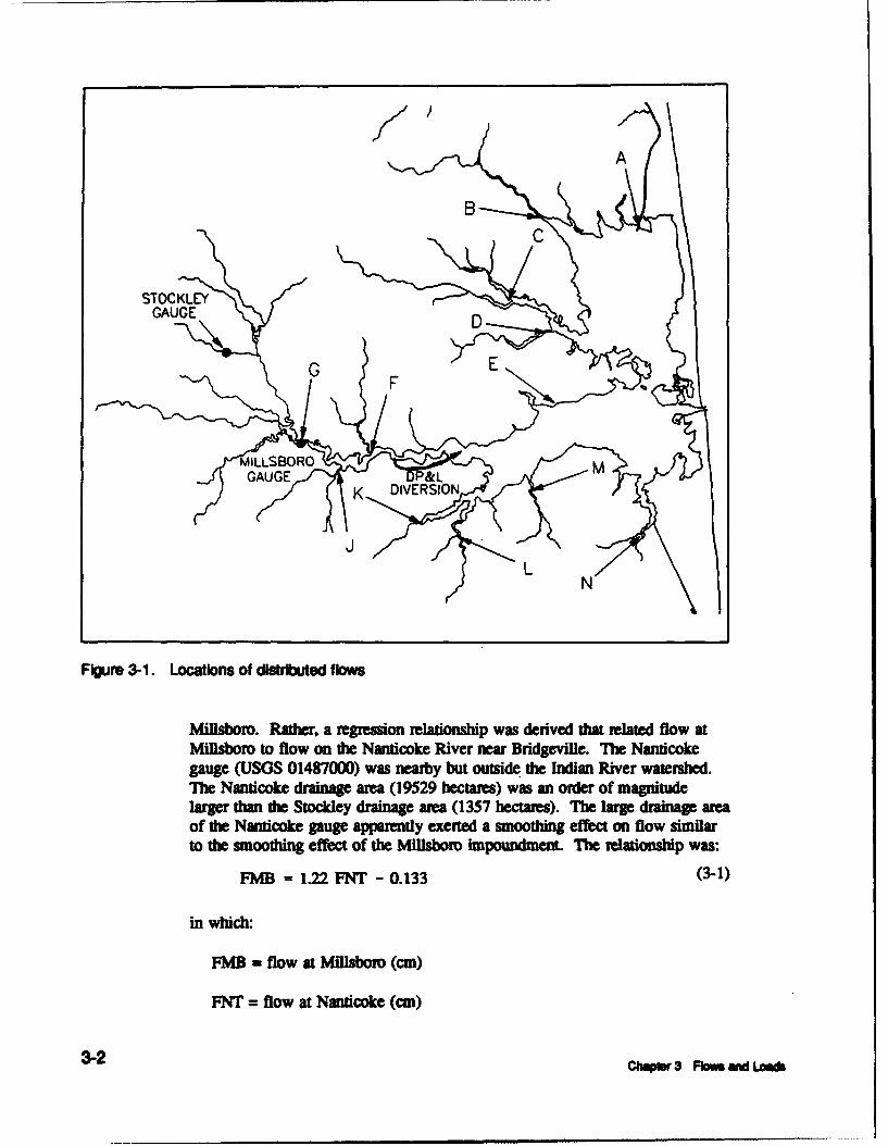
The volumetric freshwater runoff rate was one of the forcing functionsrequired to drive the hydrodynamic portion of the Indian River/Rehoboth Baymodel. Both the time series and spatial distribution of nmoff were necessary.Runoff volume was also required to compute the distributed loads of nutrientsand organic matter to the system. The drainage basin contained only onestream gauge, on Stockley Branch (Figure 3-1), active during the entire studyperiod. The strategy adopted to jet flow throughout the basin was to convertStockley volumetric flow (e.g. m sec1) to flow per unit area (e.g. cm day-1).This flow per unit area was multiplied by drainage areas of subbasins withinthe watershed to get the volumetric flow in each subbasin. Subbasin locationsand areas were obtained from Ritter (1986) who identified 16 subbasins in theIndian River/Rehoboth Bay watershed. Of these, three contributed to Mills-boro Pond upstream of the dam and were combined by us into one. Landareas draining directly into Indian River and Rehoboth Bay were named asindividual watersheds by Ritter. We allocated the direct discharge area totributary subbasins so that the total number of subbasins considered in thisstudy was twelve (Table 3-1). Flows from each subbasin were input to themodel at the discrete location (Figure 3-1) at which the subbasin tributaryentered the receiving water. Flows were updated on a daily basis throughoutthe three-year study period.

Mlllaboro Pond

Flow from the largest of the subbasins (Figure 3-2) entered the tidal systemacross the Millsboro spillway. A gauging station (USGS 0148455525)operated at the spillway during a portion of the study. Comparison of flows atStockley and Millsboro (on a per unit area basis) showed the impoundmentexerted a smoothing effect (Figure 3-3). Peak flows at MHisboro were damp-ened relative to the Stockley gauge while minimum flow from the impound-ment was higher than gauged at the upland station. Due to the smoothingeffect, the Stockley flow per unit area was not used to provide flows at

Chmr 3 Flos aW Loe 3-1

)A IBSTOCKLEY

GAUGE D

/1 ~L/S~N

Figure 3-1. Locations of distributed flows

MiUsbod. Rather, a regression relationship was denved that related flow atMillsboro to flow on the Nanticoke River near Bridgeville. The Nanticokegauge (USGS 01487000) was nearby but outside the Indian River watershed.The Nanticoke drainage area (19529 hectares) was an order of magnitudelarger than the Stockley drainage area (1357 hectares). The large drainage areaof the Nanticoke gauge apparently exerted a smoothing effect on flow similarto the smoothing effect of the Millsbor impoundmen. The relationship was:

FMB = 1.22 FNT - 0.133 (3-1)

in which:

FMB = flow at Millsboro (cm)

FNT = flow at Nanticoke (cm)

3-2 ChpWi 3 Flom wd Loa&

Table 3-1Subneus In MIdian River Rehoboth Bay Waeshd

Code sum Arm e)

A Lowes-Rohoboth Canal 3785

B Love Creek 5682

C Herring Creek 6397

D Gunea Creek 3547

E Ungo Creek 1801

F Swan Creek 5527

G Miliboro Pond 14339

J Iron Branch 5997

K Pepper Creek 4154

L Vines Creek 4027

M Blackwater Creek 3549

N White Creek 3385

16000

14000

12000

10000

6000

4000f

2000

0

Figure 3-2. Subbasin areas

€O~Mr 3 Rowm aid Look 3-3

0.7

0.6

0.4 -------- Sto dey

.• III i,o2 'I ,

0.1

JULIAN DAY SINCE JANUARY 1,1968

Figure 3-3. Comparison of flow per unit area at Stodey and MilSboro

The RW for the relationship was 0.95 for monthly-average flows.

Delmarva Power and Light Diversion

The Delmarva Power and Light Company operates a power plant on thesouthern shore of Indian River. Three once-through cooling units divert waterfrom Indian River, through the power plant condensers, and into Island Creek.Discharge water flows down the creek and rejoins Indian River downstream ofthe intake, close to the location wher the riverine portion opens out intoIndian River Bay (Figure 3-1). The cooling water diversion was included inthe hydrodynamic model. Flow through the power plant, at monthly intervals,was obtained from discharge monitoring records (DMRs) provided by theDepartment of Natural Resources and Economic Conservation. The flowdiversion was 12 to 16 m3 sec" (Figure 34). Interpolated flows wereemployed to fill gaps in the DMRs.

Relation to Groundwater Flow

Roughly 80% of stream flow in the Indian River/Rehoboth Bay watershedis base flow contribution from groundwater (Johnston 1976). The runoff perunit area records derived from the Stockley gauge included both groundwaterand overland runoff. Extension of the Stockley record to the entire watershedextended both overland and groundwater runoff volumes. Independent esti-mates (Andres 1992) have been made of the groundwater contribution to

3-4 chGwr 3 FbM Wd Los&

18.00

16.00

14.00

12.00

*--10.00

~8.00

6.00

4.00

2.00

0.00 '- - ..cc -O 00 Go W W an M, M at aý C:1 aO Cý == C -

Figure 3-4. Volumetric flow diverted through Delmarva Power and Light cooling units

Indian River/Rehoboth Bay from drainage immediately adjacent to the shore-line. Since this area was represented in our twelve subbasins, no additionalaccounting for groundwater was required.

Flows Through Navigation Canals

Canals connect Rehoboth Bay with Delaware Bay and Indian River Baywith Little Assawoman Bay. At present, no information exists on flow andmaterial exchange through these canals. As a first approximation, we assumedno net flow occurs through the canals.

Hydrologic Characterization

Runoff at the Stockley gauge during the study period is summarized inFigure 3-5. Two years, 1988 and 1990, had typical hydrographs. Flow washighest during the first half of the year and lowest during spring and fall. Thehydrograph for 1989 was unusual, however. Peak flow occurred duringAugust and flow in all months exceeded the long-term average. Recurrencerelationships (Table 3-2) indicate the flows that occurred in 1989 are exceededby less than 8% of the years on record. Flows that occurred during summer1989 are exceeded by less than 2% of the years on record. Calendar year1989 was extremely wet. By contrast, annual flow in 1990 was close to long-term median flow while 1988 annual flow was below average. Summer flows

Chpu 3 Flom and Load 3-5

4.54 Flow

3.5 L -ngTerm Mean

3

~-2.5S2

1.5

0.501I i I I I I I I I I i i g l I I I I I I I I I ! I I I

Figure 3-5. Monthly flow per unit area at Stockley 1988 - 1990

Table 3-2Hydrologic CCerizatIon I

[ Pernt o Years That Exee This One'

Twelve Months, 1988 70.2 Dry

Twelve Months, 1989 7.4 Wet

Twelve Months, 1990 54.2 Average

July - September, 1988 43.6 Average

Jul - September, 1989 1.1 Wet

July - September, 1990 39.3 Average

'Obtained from SMullen 1992

in 1988 and 1990 were similar and close enough to the median to be character-ized as "average".

3-6 Chqlr 3 Flows and Loemd

Loads

The water quality model requires nutrient and organic loads to IndianRiver/Rehoboth Bay as forcing functions for computation of receiving waterquality. Loads can be divided into three classes: Distributed Loads, Point-Source Loads, and Atmospheric Loads. Distributed loads enter the system asrunoff from the watersheds that drain into the tidal waters. Point-source loadsoriginate in industries and treatment plants along the shoreline. Atmosphericloads are deposited directly on the water surface in rainfall and as dryfall.Both the time series and locations of these loads are required for the model.

Distributed Loads

Distributed loads were computed as the product of runoff volume and con-centration of nutrient or organic substance. Runoff volumes were the same asthose used to drive the hydrodynamic model. Monthly loads were computedfor each subbasin and input to the model at the same locations as the flows(Figure 3-1). Concentrations in the runoff were obtained from analysis of the"Upland" stations in the STORET data base. Separate analyses were con-ducted for the Millsboro subbasin and for the remaining watersheds. Weconducted separate analyses to allow for concentration differences betweenfreeflowing streams and water leaving the impoundment.

Freeflowing Streams. Our analysis of the data indicated no relationshipbetween concentration and location or flow. Observations of most substancesexhibited a high degree of variability. Mean concentrations were unduly influ-enced by a few extreme observations. We characterized concentrations in therunoff (Table 3-3) as the median value of all observations since the medianstatistic is less influenced by extreme values than the mean. No temporal orspatial variability in concentration was considered except for nitrate whichexhibited a temporal pattern; concentration was generally higher in late autumnand winter than in summer (Figure 3-6). Monthly median concentrations wereemployed to compute nitrate loads.

MUilsboro Spillway. Analysis of concentrations in water leaving the Mills-born impoundment parallelled analysis of concentration in freeflowing streams.No relationship of concentration to flow or season was evident except fornitrate which showed a temporal pattern similar to freeflowing streams (Fig-ure 3-6). Concentrations were characterized as the median of all observations(Table 3-4) except for nitrate. For nitrate, monthly median values wereemployed.

Total Organic Carbon. The water quality model employs organic carbonas a state variable. Runoff observations included BOD5, but not organic car-bon. No direct conversion of BOD to organic carbon exists but empiricalrelationships can sometimes be found. We examined a data base of total

Cha•pi 3 Flmn and Loe* 3-7

Table 3-3Concentrations In Freeflowing Streams

Total TotulAmmonlum Nlrste Nitogen Phosphate Phosphorus Carbon

Mooh gmm4 gmm 4 mm4 gm m4 gm m4 W gm m4

Jan 0.1 2.98 0.88 0.11 0.03 9

Feb 0.1 2.58 0.88 0.11 0.03 9

Mar 0.1 2.65 0.88 0.11 0.03 9

Apr 0.1 2.04 0.88 0.11 0.03 9

May 0.1 1.62 0.88 0.11 0.03 9

Jun 0.1 0.86 0.88 0.11 0.03 9

Jul 0.1 0.23 0.88 0.11 0.03 9

Aug 0.1 1.13 0.88 0.11 0.03 9

Sep 0.1 1.69 0.88 0.11 0.03 9

Oct 0.1 0.39 0.88 0.11 0.03 9

Nov 0.1 1 0.88 0.11 0.03 9

Dec 0.1 2A3 0.88 0.11 0.03 9

organic carbon (TOC) and CBOD5 observations collected in freeflowingstreams tributary to the upper Potomac River. A loose curvilinear relationshipwas evident (Figure 3-7). TOC concentration at Millsboro and in freeflowingstreams was obtained visually from the figure as the TOC concentration(9 gm m-3) corresponding to median BOD5 concentration (2.5 gm m-3) in the"Upland" data set.

Point-source Loads

Thirteen point sources exist within the Indian River/Rehoboth Beach water-shed (Figure 3-8). One of these, the Lewes STP, discharges near the nofnhemterminus of the canal that connects Delaware and Rehoboth Bays. Consistentwith our assumption of no net flow through the canal, we assumed that Leweseffluent does not travel the length of the canal to Rehoboth Bay. TheRehoboth Beach WWTF and lesser point sources that discharge near the south-em terminus of the canal were included as Rehoboth Bay point sources. TheGeorgetown STP discharges into a tributary of the Millsboro impoundment.Loads from Georgetown do not require explicit treatment since they areincluded in the distributed load assigned to the Millsboro spillway. (Analysis

3-8 Chapter 3 Flows and Loads

3.-

3 -- mmasbo w

2.5

2

0.5

0-

Jan Feb Mar Apr May Jun Jul Aug Sep Oct Nov Dec

Figure 3-6. Monthly median nitrate concentration at Millsboro spillway and in freeflowingstreams

indicates Georgetown loads are less than 5% of the total load at Millsboro.)Deletion of Lewes and Georgetown leaves 11 point sources for consideration.

Flows and Concentrations. Loads from each point source were computedas the product of volumetric flow rate and substance concentration. Flow andconcenraion data were supplied by DNREC. Flow data was mostly complete,on a monthly basis, especially for the larger point sources. Flows in missingmonths were obtained by substituting flows from the same months in alternateyears. Concentration observations were sporadic, however. For some sources,data were available only for 1991 or 1992, after the study period. We foundno rational basis for assigning temporal variability to the point-source concen-trations. Mean concentration of all available observations was assigned to eachpoint source (Table 3-5). Consequently, temporal variations in computedpoint-source loads were due exclusively to variations in flow rather thanconetration.

Total Organic Carbon. The water quality model employs organic carbonas a state variable. Point-source monitoring included BODS, but not organiccarbon. Following the pattern set for distributed loads, we attempted to findan empirical relationship between the two substances. We examined a database of total organic carbon (TOC) and CBOD5 observations collected in pointsources discharging to the upper Potomac River. No relationship was evident(Figure 3-9). We selected from the data base the median concentration, 18 gmm"3, to characterize effluent TOC in Indian River/Rehoboth Bay.

Chmr 3 FoW and Lom 3-9

Table 3-4Concentrations In Millaboro Spillway

TolIT OM KMI•, Owftc OrricArmmwum Miuts i" Phouphat Phosphorms Carbon

gOm4 gmm 4 gnMm gmm4 gmm9 gfrmm 4

0.1 3.07 0.8 0.03 0.02 9

0.1 3.03 0.8 0.03 0.02 9

0.1 2.66 0.8 0.03 0.02 9

0.1 2.23 0.8 0.03 0.02 9

0.1 2A5 0.8 0.03 0.02 9

0.1 2.13 0.8 0.03 0.02 9

0.1 1.35 0.8 0.03 0.02 9

0.1 0.98 0.8 0.03 0.02 9

0.1 1.7 0.8 0.03 0.02 9

0.1 1.76 0.8 0.03 0.02 9

0.1 1.76 0.8 0.03 0.02 9

0.1 2.5 0.8 0.03 0.02 9

Delmarva Power and Light. Information and data on Delmarva Powerand Light operations were supplied by Mr. Robert Jubic of DP&L. DP&L hasseveral operations which require consideration in computation of point-sourceloads. The largest flow through the plant is cooling water for Units I - 3. Nomaterial is added to the once-through cooling water. We assumed, however,that viable algae do not survive the trip through the condensers. Code wasinstalled in the model so that algae withdrawn through the diversion fromIndian River were discharged as equivalent amounts of nutrients and organicsubstances into Iand Creek. No material was added to the cooling water,however.

Water increases in temperature as it passes through the condensers so thatdischarge temperature is higher than withdrawal temperature. Cooling of dis-charge water occurs in Island Creek before the water rejoins Indian River.Since our model does not include Island Creek we could not use plant recordsof discharge temperature. We had no way to compute the cooling effect in theCreek. Instead we used STORET data, supplemented by University of Dela-ware observations, to derive temperature differences between observationscollected near the DP&L intake and the mouth of Island Creek. Temperatureincrease between the intake and creek mouth ranged from 0.95 to 7.5 C' (Fig-ure 3-10). Average increase was 4.2 CO. Code was installed in the model to

3-10 Ch.pler 3 Fiwm and LLae

TOC VS BOD IN FREEFLOWING STREAMS

25

0 00 0

20 00

0lID 0

0 0 0

~150 0 0

0 wo 00 00a 000 0 0

0 M 0 OD 0 0 0 010 C1@ 0 D

- a) 0Mo0 0 0

0 •> 00 0 0OODO 0 so

5 00 0 00 O0 0 0

0

0 0 0 10 1 2 3 4 5 6 7 8 9 10

BOD (MG/L)

Figure 3-7. Total organic carbon versus CBOD5 in freetlowing streams tributaryto the Potomac River below Washington, DC

increase by the mean value temperature of water diverted through the DP&Lplant.

A snall portion of condenser discharge is diverted into the Unit 4 coolingtower. The tower operates through evaporative cooling so that substance con-centrations increase in the cooling water. When solids concentration in thewater increases by a factor of three to four, the tower is "blown down"(emptied) via Discharge 027. Total nitrogen concentration in "blow down"water is three to four times higher than intake water (Figure 3-11), consistentwith the increase in solids. Nitrate concenmion increases by an order ofmagnitude, however, and total Kjeldahl nitroge concation decreasesdespite the evaporative water loss. The data suggest mineralization of organicnitrogen and subsequent nitrification occur in the tower. To account for thiseffect we convened -app rate amounts of organic nitrogen in DP&L diver-sion water (-30 kg day' ) to nitrate. No net addition or subraction of totalnitrogen was considered, however.

For two of the three study years, 1988 and 1989, phosphorus detergent wasadded to the cooling tower water. Monthly data on phosphorus use was pro-vided by DP&L. We added these phosphorus loads to the DP&L diversionwater. Phosphorus use at the plant ceased after Decenber, 1989.

No data was available to assess the effect of the cooling tower on totalorganic carbon. We assumed no net addition or change through the tower.

Ow s 3 Pow WKI Lot 3-11

sip

ATLANTIC

£ \OCEAN

Figure 3-8. Point sources in the Indian River/Rehoboth Bay drainage basin

The DP&L plant has a small sanitaiy facility (Discag 028). This facilitywas considered separately from the cooling water. Analysis amd -treannet ofthe sanitazy facility was identical to the other POint sources in the system.

Atmospheric Loads

Data to compute atmospheric nuttient loads, collected at nearby CapeHenlopen Delaware, were supplied by Dr. Joseph Scudlark of the University ofDelaware. Mean ammonium load in rainfall was 2.6 kg N heczare"' year1m.Mean nitrate load was 14.1 kg N hectare"' year". Organic nitrogen load wasestimated as 15% of the inorganic load. No amnosphenc load of phosphoruswas detected. A "rule of thumb" in consideration of annosphetc loads is thatdiyfall. difficult or impossible to measure, equals wetfall. To account fordryfanl, the measures and estimates of nitrogen in rainfall were doubled.Atmospheric loads were applied uniformly throughout the study period to all

3-12 r.,•sREHOBOTHo

Table 3-5Point-Source C cntralons

I I ToullTot IidW l Oinc ft

Amnmkium ue Mro Pho"s Phoep. agumR gm ' l gum 4 grnm 4 gm 4 gm R

Delaware 72 17.3 7.2 3.8 0.6 18SeashoreState Park

Frankford 9.86 22.7 9.86 5.5 1 18ElementafySchool ___

Town of 7.1 2.6 8.7 2A 0.3 18Millsboro

Townsend's 1 21.8 6 0.1 0 18Inc.

Vlmssic 0.06 3.1 1.36 0.064 0.066 18Food

Colonial 9.7 6.85 9.7 2.2 OA 18East MobleHome Pk.

Rehoboth 0.95 0.62 5.76 3.46 0.61 18BeachWWTF

Delaware 1.15 28.8 1.15 4.25 0.75 18StateHousingAuthority

Bayshore 7.2 17.3 7.2 3.8 0.6 18MobileHome Pk.

Colonial 7.9 10.7 7.9 3.1 0.5 18Estates

Delmarva 0.9 15.2 3.1 1.26 0.14 18Power andLight (02)

portions of the water surface. No attempt was made to account for spatial ortemporal variations in load. The total atmospheric nitrogen load to the watersurface was 765 kg day'.

ChWtsr 3 Fbm and L___ 3-13

TOC VS BOD IN POINT SOURCES

35

030 0

000 0 0 0

0 0 0(000 0 0

-J 0 0"-.20 0 0 0 0- 0 0 0 O

0D 00815 0 0 0 00 o0 00

o00 00 O0 0

0 0

10 o0 0

0

5

0O0 1 2 3 4 5 6 7 8 9 10

BOD (MG/L)

Figure 3-9. Total organic carbon versus CBOD5 in point sources discagito the Potomac River below Washington DC

Summary of Loads

Distrilbuled Lauds. A summary of the subbasin loads, averaged through-out the study period (Table 3-6, Figure 3-12). indicates that nitrogen loads aredist'ibuted roughly in accordance with subbasin area. Millsboro is the aresubbuin and the largest distributed nitroge source. Millsboro is also thelargest distributed phosphorus sourc (Figure 3-13) but is not as dominant asfor niutrogm. The relatively large distributed pophorus loads from the free-flowing subbasins occur because total phosphorus ce aion attributed tothese bsins is nearly thmr times larger than concentrhatd, at Milloboro. Thecoceatio disparity suggests phosphorus settling occurs in the pond but theapparent differences may also be an artifact of the data analysis. Alternatetreatme-ns of the data can be conducted that indicate no difference in phospho-rus coM-entration. Total organic carbon loads from the subblins (Figure 3-14)reflect exactly the relative areas of the basins since concentr1i is uniformacross all subbasins. Millsboro is the largest distributed source of total orgpccarbon.

Poin-Source Loads. A summary of the point-source loads. averagedthroughout the study period (Table 3-7), indicates that the Townsend's plant isby far the lrgest point source of nitrog (Figure 3-15). Rehoboth Beach

3-14 chper 3 Fbn * L•&a

40EUpetmam

35 o Dowratm30

25

20

15 "

10

0

24- 30- 24- 28- 25- 30- 31- 11- 16- 13- 24-Apr- May- Jul- Aug- Sep- Apr- M"a jJun- Ju Aug Sep-89 89 89 89 89 90 90 90 90 90 90

Figure 3-10. Temperature difference between DP&L intake and discharge to Indian River

7

TotlENNitate're

5

4

3

2

Total N Nitrate I1CN

Figure 3-11. Nitrogen concentrations in cooling tower intake and discharge

Chwein 3 Floms aid Lamb -1

Table 34Mw Dlibutmd Loads 19•-190

ToM Orpdl7o1 moW ToM Phoephmuos

su k9 dW It kdW 119 d

Lewes-Rehoboth Canal 96 5.16 332

Love Creek 155 8.34 536

Herring Creek 177 9.53 613

Guinea Crook 88 4.76 306

Lingo Creek 39 2.13 137

Swan Crook 155 8.37 538

Iran Branch 170 9.15 588

Pepper Creek 113 6.07 390

Vines Crook 109 5.85 376

Blackwater Creek 94 5.05 325

White Creek 89 4.78 307

Millsboro Spillway 717 11.90 2143

Total 2000 81.09 6591

WWTF dominates the phosphorus point sources (Figure 3-16) and is thesecond largest nitrogen contributor. Town of Millsboro is the second largestphosphorus contributor followed by the DP&L "blow down" water (027).Note that the loads for DP&L are averaged across the three-year study period.For two years, 1988 and 1989, the DIP&L load was roughly equivalent to theTown of Millsboro. The DP&L load in 1990 was zero, however, and does notcurrently exisL Townsend's and Rehoboth Beach also lead in point-sourcetotal organic carbon (Figure 3-17).

Relative Loading. Distributed loads comprise the largest nitrogen sourceto the system (Figure 3-18). In 1988 and 1990, largest nitrogen loads occurredin the first six months. This pattern reflected both the hydrograph and thetemporal panem in nitrate concentration. In 1989, the extremely wet summerwas mirrored by unusually large nitrogen loads in the summer months. Atmo-spheric nitrogen loads are the next largest source. During the dry summermonths of 1988 and 1990, periods of high algal and low dissolved oxygenconcentaton, atmospheric loads equaled or exceeded distributed loads. Pointsources are the least of the nitrogen loads although point-source loadsapproached distributed loads in magnitude during the dry summer of 1988.

3-16 •3 Floms md Loft

8.000

700.00

600.00

4 400.00

300.00

200.00

100.00 F0.00-0

Figure 3-12. Mean total nitrogen load! from subbasins

12O0

10.00

8.00

6.00

2M0

0.00

Figure 3-13. Mean total phosphorus load from subbauins

_____ o wd~o 3-17

2500.00

2000.00 !:i

4.•1500.00...

ON FFilII I

Figure 3-14. Mean total organic carbon load from subbasins

Distributed loads are also the largest source of phosphorus (Figure 3-19).The distributed phosphorus load mirrors exactly the hydrograph since no tem-poral variation in phosphorus concentration is considered. In 1988 and 1990,largest phosphorus loads occurred in the first six months of the year. In 1989,largest phosphorus loads occurred in summer due to the unusually large sum-mer flows. Point-source phosphomrus loads are less than distributed loadsalthough during the dry summer of 1988 point-source loads exceeded distri-buted loads. The point-source loads exhibit a periodicity. Highest loads occurin June, July, and August due to flow variations at the Rehoboth Beach facil-ity, the largest phosphorus point source. Flows in summer months are three orfour times greater than in winter months.

As with nitrogen and phosphorus, distributed total organic carbon loadsexceed point-source loads (Figure 3-20). The distributed loads dominatethroughout the year in dry or wet hydrology.

Comparison to Previos Estimates. "Desktop" estimates of loads toIndian River/Rehoboth Bay for "Wet", "Dry", and "Normal" years were com-pleted by Ritter (1986). We compared our loads to the previous estimates.Our loads for 1988, 1989, and 1990 were compared to previous estimates for"Dry", "Wet", and "Normal" years respectively (Table 3-8). Our total nitrogenloads are comparable to previous estimates but average roughly 15% less.Comparison of loads by category indicates rough equivalence of distributed

3-18 GG 3- -O Lomb

Table 3-7Mm Point-Source Loads 1968-1990

Total Mtgan P11ouphrus Caubonsouo kgday Itoday kgd"

Delaware Seashore State Park 1.37 0.30 1.23

Delmarva Power and Light (027) 0.00 1.64 0.00

Frankford Elementary School 02.7 0.05 0.15

Town of Millsboro 11.87 2.84 18.91

Townsend's Inc. 145.23 0.52 94.04

Vlassic Food 4.79 0.14 19.34

Colonial East Mobile Home Pk. 1.14 0.18 1.25

Rehoboth Beach WWTF 25.76 16A3 72.67

Delaware State Housing 0.94 0.16 0.57Authority

Bayshore Mobile Home Pk. 0.26 0.06 0.24

Colonial Estates 0.90 0.17 0.87

Delmarva Power and Light (028) 0.53 0.04 0.52

Georgetown' 34.37 0.48 27.18

Lewes STP2 32.29 7.77 37.50

Total Contributing Point Sources 193.06 22.54 209.77

' Load from this point source is included in the distributed load from the Millsborosubbasin.2 Not considered as a load to Rehoboth Bay. Shown only for comparison.

nitrogen loads. Comparison of other categories indicates significant differ-ences, however. Our point-source nitrogen loads are only a third of previousestimates. This difference may be due to a reduction in point-source loadssince the previous estimates were completed or else improved quantificationdue to availability of additional, contemporary data. Our atmospheric nitrogenloads are triple the previous estimates. In view of the nature and extent of theCape Henlopen data base, current estimates must be regarded as the best avail-able. The differences in current and previous estimates of point-source andatmospheric loads offset. Total nitrogen loads would be nearly equivalentexcept for additional loads considered by Ritter. The excess in previous esti-mates over current estimates is due to septic tank loads considered by Ritterbut omitted from this study.

Chapter 3 Flows and Los& 3-19

160.00

140.00

120.00

100.00

z 80.00

60.00

40.00

20.00 ITT

0.00 " 4JZt _ ' -- ,

ISI

Figure 3-15. Mean total nitrogen load from point sources

18.00

16.00

14.00

12.00

910.00

S8.00

6.00

4.00

2.00 - 779 I 1 !I2.00

j! - j |

Figure 3-16. Mean total phosphorus load from point sources

3-20 ch~wr 3 Fb= and Load

100.00

90.00

80.00

70.00

~60.00850.00

S40.00

30.00

20.00

10.00

0.00

Facure 3-17. Mean tuu. , nanic carbon load from point sources

6000

• PtSrcN

00 ----- --NonPtSrcN /

4 Aft,,mphem N

3000 a \I a a a a a ,,

a a ia a I ,

2000a a1o000•f "l \

08 8a a 3B3 a1 83 or sr or a aor or :S tSt9 t5 tS tSI I I

Fi 3-18. Tiam series of p - e, d i d, and er i a n lds

ChWW Rbw wi Lom 3-21

300

20PtSrcP

--------. Non Pt Src P

200 1 aN2o0 A

so \

,,P a II S

loo , ' " , , / ,

I s S I I a a a g a a I S 6 I tI I I I tI I I a s a a a

Figure 3-19. Time series of point-source and distributed phosphorus loads

250M0

PtSriTOC20000

SoNPtSrcTOC

Sm'

I

"a ' 'SV '

\ / -./

a a , , o , ,as i , , a

Figure 3-20. Time series of point-source and distributed total organic carbon loads

3-22 Ow.a 3 Pam Od Lea*

Table 3.8Comparson of Loads

lmDry 1989 wet 1Iwo Nobmw

9Bo8 k dy kg day" k4 CWy" k% dey" k0 dWy IQ dW/

Point 209 634 204 634 166 634Sources

Distributed 1300 1091 2683 3240 2017 2186

Loads

Atmospheric 765 171 765 342 765 174

Other 0 515 0 515 0 515

Total 2275 2410 3652 4730 2948 3509

Peplhospho[s IM Dry 169 Wet 1990 Nom

Point 24 72 23 72 21 72Sources

Distributed 48 52 121 159 74 104Loads

Atmospheric 0 11 0 21 0 16

Other 0 14 0 14 0 14

Total 72 149 144 267 96 206

Current estimates of total phosphorus loads are less than previous estimatesfor all loading categories. The sum of all current loads is half the previousestimate. Differences in distributed loads are small relative to the uncertaintyin the load estimates. Differences in point-source and atmospheric loadinglikely occur due to the availability to us of additional, contemporary data. Aswith nitrogen, phosphorus loads from sources considered by Ritter, primarilyseptic tanks, were omitted in this study.

3-23Chalpter 3 Flows and Loads

Chapter IV: Description of theHydrodynamic Model

The numerical hydrodynamic model CH3D (Curvilinear Hydrodynamics inThree Dimensions) was used to provide detailed hydrodynamic flow fieldinformation as input to the water quality model. The basic model was devel-oped by Sheng (1986) but was modified extensively in its application to theChesapeake Bay study (Johnson et al. 1991). These modifications includeimplementing different basic numerical formulations of the governing equa-tions as well as substantial recoding to obtain a more computationally efficientmodel. Physical processes impacting circulation which can be modeledinclude tide, wind, river inflow, and the effect of the earth's rotation (i.e.,Coriolis effect).

A key attribute of C113D is its ability to define a basin in a boundary-fittedcoordinate system, allowing grid coordinate lines to conform with irregularcoastal features, such as a shoreline or navigation channel. The solution algo-rithm employs an external-internal mode-splitting technique. In the externalmode, finite difference approximations of the vertically-integrated Navier-Stokes equations are solved, yielding water surface elevations and depth-averaged x- and y-directed unit flow rates. This information is then processedin the internal mode to determine the x-, y-, and z-directed velocity distribu-tions through the water column. Because the Indian River-Rehoboth Baymodel application is a two-dimensional, depth-averaged (i.e., external) modeapplication, the internal mode is not discussed in this chapter.

This chapter describes the governing equations used in CH3D and the for-mulation of bottom and surface shear stress terms as well as the Corioliseffect. The process of transforming and non-dimensionalizing the governingequations is discussed and finite-difference approximations of the governingequations are presented.

Governing Equations

The hydrodynamic equations used in CH3D are derived from the classicalNavier-Stokes equations formulated in a Cartesian coordinate system

ch~pr 4 Des"a on to Ue y•-Ync MOM 4-1

(Figure 4-1). Assuming that the vertical water accelerations are small in com-parison with the gravitational acceleration (i.e., hydrostatic pressure conditionsexist) and that the fluid is homogeneous and incompressible, the depth-averaged approximation yields the following in-plan, two-dimensional form ofthe governing equations:

x-Momentum

au a (uu aUvU ~TU UVU •.• (_f) + gH aS-'m- +T

2U ax u 1 (=0_f + + A +c +B2 BzU =I 0-p --p HI•+-y]p-'r+i,•

y-Momentumn

av+a (UV +a (VV +g as +J(2)

"- C+ Toy ++A f 2V + a)2V+ lp 0A- - Jpa p ~ 2 -ý

Continuity

as + + av 0 (3)

where

x, y, t = independent space and time variables

U, V = unit flow rate components in the x- and y-directions, respectively

H = total water depth (h+S)

S = water surface displacement measured relative to an aibitraydatum

h = static water depth measured from the same datum

g = gravitational acceleration

4-2 cUVr 4 Desaiption of U* Hydodynwnc Moft

z x

Figure 4-1. Cartesian coordinate system definition sketch

f Coriolis parameter

, cs = surface shear stress in the x- and y-directions, respectively

Bz', -%y = bottom shear sums in the x- and y-directions, respectively

p = water density (assumed to be constant)

AH = generalized dispersion coefficient

p pressure

Bottom Shear Stress Formulation

CH3D uses the following quadratic expression to represent the bottom shearstress in the x-momentum equation:

'Co 9 C U2 U (4)+V

where

C4 = Mezy's resistance factor

ChgmW4 Dsadpdon of w Hydrodwrmic Mod-3

A similar expression is used fory, in the y-momentum equation.

Rather than specifying the Chezy resistance factor, Manning's n, which isindependent of depth, is input to the model. These coefficients are relatedthrough the following equation:

H 11

c, W-T (5)

In addition, CH3D has an option for designating Manming's n as a fuction ofdepth to specify changes in bottom roughness at different water depths.

Surface Shear Stress Formulation

The surface shear stress , is formulated as:

', = p. CDIWIW (6)

where p, is the air density, W is the wind velocity, and CD is a dimensionlesswind drag coefficient. CH3D uses the wind drag formulation presented inGarran (1977):

CM - (0.75 + 0.067o)) (7)1000

where M is the wind speed. This formulation requires wind speeds specified inunits of meters per second. An upper limit of 3.0x10 3 is applied to this coeffi-cient. Thus, for wind speeds greater than 65 knots, a constant drag coefficientis applied.

Corlolls Effect

Although it is not a true force, the Coriolis effect accounts for the apparentdeflection in a fluid's trajectory that is induced by the rotation of the Earth.The Coriolis parameterf is expressed as:

f avsm (8)

c4-4 4 Des@aclp of oIe HdW~mw Mod

where v is the angular speed of the Earth's rotation (7.292 x 1o0 rad/sec) andX is the latitude of the study area (38 deg 36.5 min).

Non-Dimensionalization of Governing Equations

The dimensionless form of the governing equations are used to facilitaterelative magnitude comparisons of the various terms in the governing equationsand to minimize the effects of round-off errors during computations. Thefollowing dimensionless variables are used:

(u, v, w) = (u, v, wX,/Z)/U,

(x, y" z ) = (x, y, zX/Z)/X

(TI, T;) = (T7. r•)OPfZrUr

t*=f

S = gS/fux, W S/S,

A; AH/Aw

These definitions yield the following dimensionless parameters in the govern-

ing equations:

Froude Number, F,.= U,/(gZ,)

Rossby Number R = UtX,

Densimetric Froude Number FrD = F, / Fe

where

S= (p, - pd/po

U,, p,. X,, 7.,, Am,, and K&, are arbitrary reference values of the velocity,density, length, depth, dispersion, and diffusion.

Using the dimensionless variables (asterisks have been dropped) and theparameters previously defined, the vertically integrated equations constitutngthe external mode are:

Chir 4 Dlpflto• to iHydao rmicl Mod4-5

-v T ,Tx [+(EHJ+(AH A 0 iJ (9)

+S R t. (H)2~

Transformation j+ E of a Goerin Eqa tions (H (0

thtransforrmation of itGove ning e quationsinoan-hooa

curvilnear or boundary-flued coordinae system (aj'). Both independent (e.g.,x, y) andi dependent varibles (e.g., U, V) in the governing equatons amc

ChWb 4 Desalpelo of sI* Hydymio~wf McMs

transformed into the (4m'l) curvilinear system. CH3D employs contravariantcomponents (as opposed to covariant components) in the transformation of thegoverning equations, therefore velocities are defined perpendicular to a cellface, as opposed to parallel to a cell face.

The flow rate components in physical space (i.e., U() and V(j)) are relatedto the contravariant components (i.e., U' , vU, Vi) by the followingequations:

U(O = .1U 9 12 Vi (12)

VQ)J 921 U .= Vj (13)

where g, is the metric tensor defined as:

2 2.gii X= "V '

or

11g 9l12 (15)

Lg# 9 1 g.j

and I g I is the determinant of the metric tensor g,:

I1 I = s,192 - 81282 (16)

Whereas scalar quantities in the physical plane are identical in the transformedplane, all spatial derivatives containing these terms must be tuansformed. Thesurface slope terms are transformed as follows:

4-7

as 9 11W g 12 aS (17)

as 921 aS 22 CS (18)W;~ Xs F

where g u are inverse metric tensor components:

2 2 Yy 1J92

or

g# " 11 12(20)

g 21 9 22

The mrnsfoned governing equations developed by Sheng (1986) are asfollows. The inertial and diffusion terms in contravariam coordinates are quitelengthy and thus are omitted in this report However, these terms are pre-sented in onson et aL (1991).

E-Momentum

e-.RInerda" + H 11 + g 12 912 U

gRg(g-U2 + 2g2UV + 8221•,)" (21)

4E,,Dt, ÷on + 2 a 9 110U =0

4-8 ChapW4 Descp of o mn e oyrui MKW

i + Rninersia ÷H 21 + +

12 .2 - 2 o2 ( 2v÷g.) v (22)

+ E H D wffiion* Fr+2 1 + 2 J 0

Continuity

"- ÷Igu) + TII V 0 (23)

where

U.V = contravariam unit flow rate components in the transformedplane (superscripts have been dropped for convenience)

I g1 = determinam of the meric tensor, I g , at an S-point(Figure 4-2)

IguIIgI = determinanit of the metric tensor, II , at a U-face and V-face,

respectively

U = average x-direction unit flow rate at a V-face

V = average y-direction unit flow rate at a U-face

Finite Difference Approximationsof Governing Equations

The finite difference approximations to the governing equations are basedon a Eulerian system where the velocities and water surface flucuations arecomputed at discrete locations within the flow field. A network of grid cells isused to define the parameter locations. A representative grid cell in compu-tational space (,Tj) is shown in Figure 2. In this staggered grid, the watersurface fluctuation is defined at the cell center (iJ), 4-direction unit

CWW 4 DeSalp of Ohe HY*Vdpm*,i Model 4-9

flow rates (U) are defined atthe "west" (ijQ) and "east"(i+)-j) cell faces, and theTI-direction unit flow rates

VL,J.x (V) are computed at the""south" (ij) and "north"(ij+l) cell faces. The finite

Q -. ,j .--- difference approximations of!, the governing equations

A -follow. Note that the conti-%J nuity equation is split into

two parts. The sum of theseequations is the original

- x continuity equation.

Figure 4-2. Variable positions

E-Momentum

R. * -- UI -i R _ S iIU* - ij + S* S*\i

+ Hg I S ji112 - i-1/2.j-1f2 g12 2 - - (24)

+ ORo(FRC)Ui* + (I-O)R0 (FRC)Uij + EHDi ÷ 0 D gj ij FrD2 2

Ro 2 -lR R

(1-0))rDo2 glj Pi1Di R° H 2 g 12(. i-l2,j+It2_- Pi-/2j-l/ = 0FrD2 2 FrD2 2Al

where

n = previous time level

* = intermediate time level

n+I = solve for this time level

4-10 Chtspr 4 Dle:sa of ft Hyeftdp~ c Model

9 = weighting factor between successive time levels

I = inertia

FRC = friction

D = dispersion

n-Momentum

"' "+ Rob! + Hg* 9+tjJ2iI~-1 Hg2 I qJ ijJ1

At___ _ Ij VAll

(1~O)~22IjJ 1 9 11 = 912.

+ (1-) 0 FO + E, U.+ tn H+ 21.2R.5.P(FlJCfl.

ft+ n.1 (At 2

R0 H2 . +~ - (1E 21 H2 P1,-l - p'-Itvj5i1

FrD2 Fr,,2 2 g Ai

E-Continuitv

Ig. +f-uO Igm I 'u~l - Ui',At Ngis wg~

']g, I An)

Chqab 4 DUWWMUO of 61W Hj*4Wt~oyu MOdW -1

li-Continuity

C +1 "I ( n.i +1 Ig I ('Vil _ Vi- S. I 0 I V +0 0"j. nAt Tg;T Ali )~ -0)

19JI _ij _ - vij _ (27)

The computational procedure used in CH3D is based on an AlternatingDirection Implicit scheme (Roache 1976). Using this method, the 4- andil-momentum equations are solved separately, and each calculation in time ismade in two stages. In the first stage, the 4-continuity and 4-momentum equa-tions are solved along each row of the grid to progress from time level n to anintermediate time level *, indicated by superscript *. The t-direction unit flowrate components and water surface fluctuations are solved implicitly, and theii-direction unit flow rate components are supplied from time level n. The4-direction unit flow rates from this step represent those at time level n+1,whereas the water surface fluctuations are only an approximation to those attime level n+l. The Q-direction unit flow rate components remain at timelevel n. In the second stage, the n-continuity and Ti-momentumn equations aresolved along each column for the Tl-diTection unit flow rates and the watersurface fluctuations at time level n+l. 4-direction unit flow rate componentsare supplied from the first stage calculations.

As shown in the finite difference approximations to the governing equations,a weighting factor 0 is used to place the water surface slope and bottom fric-tion terms between time levels n and n+l. When the weighting factor equals0.0, these terms am evaluated at the previous time level n (explicit treatment),whereas when the weighting factor equals 1.0, they are evaluated at the newtime level n+I (implicit treatment). Usually a value between 0.0 and 1.0 isused.

4-12 Chmplr 4 Descroon of to. K drodynamc Model

Chapter V: HydrodynamicModel Application

In this chapter, the application of CH3D to the Indian River Bay-RehobothBay system is described. A discussion of numerical grid development and thebathymetry used to represent the study area is given. The model calibrationand validation procedure is presented, including a discussion of boundaryforcing conditions used in the model and an analysis of model results.

Numerical Grid Development

CH3D uses a non-orthogonal, boundary-fined grid to represent the limits ofa study area. Using a boundary-fitted grid allows coordinate lines to conformto the irregular boundaries of land masses. In this way, the delineationbetween each bay and the surrounding land can be made. Similarly, the delin-eation between an island and the surrounding water can be made. Note thatCH3D does not contain an adaptive gridding algorithm, therefore there is nomeans to allow for flooding and drying of low-lying areas. To maintain theappropriate water volume in the system, active cell volumes in low-lying areaswere increased.

The boundary-conforming grid used for the Indian River Bay-Rehoboth Bayhydrodynamic study was constructed using program Eagle (Thompson 1985).The 73 x 68 cell grid generated by Eagle contains approximately 2000 activecells with cells concentrated through the inlet and Middle Island areas (Fig-ure 5-1). Cell sizes through the inlet were approximately 30-m by 120-in inthe north-south and east-west directions, respectively. Cell sizes near the Mid-dle Island area were as small as 60-m by 120-in in the east-west and north-south directions, respectively. A 1988 hydrographic survey of the Indian RiverBay-Rehoboth Bay system conducted by the U.S. Army Engineer District,Philadelphia provided the necessary bathymetric information. This informationwas translated to a depth in each grid cell by applying a 3-point linear interpo-lation scheme to the dam. Depths in the dual bay system arc generally lessthan 2 m mean low water (mlw).

ChpWh 5 Hyerdynamic Modu AppWaft 5-1

z

CD

5-2 ChmpWs 5 Hy&odynamic Moda Applicaton

Model Calibration and Validation

The purpose of the calibration procedure is to insure that the model accu-rately predicts hydrodynamic conditions within a given study area. The accu-racy of model results is greatly influenced by the accuracy of boundary forcingconditions, representation of the geometry of the study area (i.e. bathymetryand land/water interface), and to a lesser degree, the choice of certain "calibra-tion" parameters (Mark et al. 1993). In the calibration procedure, these para-meters are adjusted to obtain the best agreement between model results andmeasured field data. In essence, if the study area is accurately depicted withthe numerical grid and the boundary conditions are correct, model results willbe "in the ballpark" and the small adjustments to calibration parameters are ameans of "fine-tuning" model results.

The purpose of the validation procedure is to confirm that the calibratedmodel can replicate hydrodynamic conditions independent of the conditions forwhich it was calibrated. In this procedure, the model is applied without anyadjustment to the calibration parameters. A good comparison between modelresults and measured data in the validation process means that the modelshould accurately simulate hydrodynamics for other time periods.

The time periods selected for model calibration and validation for theIndian River Bay-Rehoboth Bay system were time periods when there wasavailable field data for comparison to model results with sufficient length ofrecord and sufficient spatial extent to cover the model domain. Another factorinfluencing the time periods selected was the fact that the hydrodynamic modelresults were used to supply flow conditions to the water-quality (WQ) model.Therefore, the hydrodynamic model should be tested over a time-span consis-tent with the transport of contaminants within this system. During a low flowtime period, river discharges may lack sufficient momentum to flush contami-nants from the system. During extreme events, large oscillations in the watersurface and/or high river discharges can provide sufficient momentum to trans-port contaminants. Because of the importance of these factors, the model wascalibrated and validated for a cycle of 7 days.

Calibration Overview

CH3D was calibrated for the Indian River Bay-Rehoboth Bay study area forthe one-week time period 29 June - 5 July 1988. Both water surface elevationand velocity data were only available for this time period. Water surfaceelevation data were also available at all tide gauges from 1 October -31 December 1988 and comparisons were made for one week during this timeperiod (14 - 20 October 1988) as part of the validation process.

The open boundary in Indian River Inlet was driven with a time series ofwater surface elevation recorded by the tide gauge adjacent to the U.S. CoastGuard Station (T5 in Figure 2-1). The grid boundary location was selected tocoincide with the gauge location. However, grid cells in this region are

Chapter 5 Iydrodynamc Model Applico 5-3

approximately 120 m wide and therefore "precise" placement is considered tobe within 60 m of the actual gauge location. In addition, the tide gauge isattached to a pier in the Coast Guard Boat Basin and is therefore somewhatsheltered. Because the influence of these factors is not known, water levelswere not adjusted in phase or amplitude to account for these factors. As aconsequence, water surface levels and velocities computed by the model maycontain phase errors of several minutes.

Tide data were collected at the USCG Station at 15-minute intervals, how-ever, water levels were supplied to the model at a 1-hr interval using a lowlowpass (LLP) filter on the recorded time series. Water levels were linearly-interpolated by the model for each time step between the I-hr input values andwere uniformly assigned to every cell on the open boundary. No water surfacelevel gradient was imposed along this boundary.

Note that after completing the initial calibration procedure, a simulation wasmade using the original 15-min interval tidal data for the inlet boundary forc-ing function and the results were not altered significantly. Therefore, using the1-hr filtered data was appropriate.

The time-history of wind speed and directions used in the model wererecorded by the Delaware Power and Light (DPL) wind anemometer. Thesedata were selected over wind data at the "old" USCG station because the DPLrecord was more complete. Short time periods missing from the DPL recordwere linearly-interpolated between recorded values. DPL data for 30 - 31October 1988 were extremely high, which when used as input to the hydrody-namic model caused grid cells to become dry, thus leading to model instabili-ties. After consulting with DPL personnel, it was determined that theseextremely high wind velocities were inappropriate and were adjusted to morereasonable estimates for that time period. Wind data were supplied to themodel at 1-hr intervals and were linearly-interpolated for time steps betweenthe 1-hr input values.

Discharge data were available from 1 January - 30 September 1988 forVines Creek and Millsboro Pond (at the head of Indian River). Flows atremaining locations throughout the system (Figure 3-1) were estimated by theratio technique described in Chapter 3. Estimation techniques were also usedto complete the Vines Creek and Millsboro Pond datasets outside the period ofrecord. Discharge data were provided by USGS as daily average flow rates,therefore model input consisted of one flow rate for each day of the simula-tion. Flow rates were updated at each time step of the simulation by linearlyinterpolating between daily values.

Data available for comparison with model results included:

1) a time series of water surface elevations recorded at each of thefollowing USGS stations (Figure 2-1):

5-4 Chapler 5 Hydrodynaniic Model Appliculti

a) Vines (TI)b) Potnets MT2)c) Massey (T3)d) Dewey (T"4)

Water surface elevation data were collected at 15-minute intervals. Waterlevel data collected at the USCG station were used to drive the inlet boundarycondition and therefore could not be used for comparison to model results.

2) currents speeds without directions collected at four locations nearMiddle Island (CM1, CM2, CM3, and CM4 in Figure 2-1).

Calibration Conditions

The hydrodynamic model was used to simulate the year 1988 so that theWQ team could begin simulations with the water quality model. The actualcalibration period, however, was only 153 hours (29 June 1500 - 5 July 2400).Data were available at all four tide gauges and current data were also collectedfor 25 hrs at the 4 velocity stations (30 June hr 0600 - I July hr 0700) duringthis time period. Data at the four tide gauges showed a variation in rangefrom a low of 0.6 m at the Dewey gauge to a high of 1.1 m at the VinesCreek gauge. River discharge for the calibration time period was extremelylow. The Millsboro Dam flow rate was 0.76-0.91 m3/sec and the Vines Creekflow rate was less than 0.03 m3/sec. Peak flow rates for 1988 were approxi-mately 5.66 m3/sec at Millsboro Dam and 2.83-4.25 m3/sec at Vines Creek.Winds during the calibration period were 1.3-5.8 m/sec generally from a north-erly direction.

Calibration Procedure

Calibration was achieved primarily through adjustments to the bottom fric-tion coefficient, Manning's n. Initially a global bottom friction coefficient wasspecified throughout the grid and the model was rin repeatedly with differentglobal values (0.020-0.035) to determine an approximate value of n. The bestglobal value was determined by comparing model predicted water surfaceelevations to measured water surface elevations at the four tide stationsdescribed previously. To achieve the more difficult task of replicating watervelocities, the global bottom friction coefficient was refined and tested over anarrower range of values. In the last stage, Manning's n values were adjustedlocally in shallow regions to account for increased friction drag in these areas.The best comparison between model results and measured data was achievedwith a global Manning's n of 0.025. Shallower areas (less than .3 m) wereassigned a friction value of 0.045.

Chqtr 5 Hy'ordnmic Moa Appicati5-5on

Analysis of Calibration Results

Water Surface Elevation

The model accurately reproduced the amplitude of the water surface leveltime histories recorded at the Vines Creek, Potnets, Massey, and Deweygauges, however, the model consistently leads the prototype data by 30 min atall gauges (Figures 5-2 through 5-5). The modeled tide travels too quicklyfrom the inlet to the gauges. Scatter plots of predicted versus measured watersurface levels show the typical elliptic shape indicative of a phase shift (Fig-ures 5-6 through 5-9). The root-mean-square (rms) error at the Vines, Pomets,Massey, and Dewey gauges was computed to be 7.1, 8.3, 3.0, and 2.7 cm,respectively. A thorough search for the cause of this discrepancy led to manyinteresting possibilities.

First, water surface level data computed by the model is written to an out-put file at an interval of 30 minutes -- the exact phase discrepancy. Althoughthis seemed to be a likely source for the discrepancy, it was not the cause inthis case. The model was run with an output interval of 15 minutes, and theresults were identical to the previous results. Another possibility for the dis-crepancy was data interpretation, i.e., a plotting error. Rather than plotting theresults, the actual values produced by the model were evaluated and comparedwith the prototype values, and the discrepancy was real.

Interestingly, all four gauges are consistently out of phase with the proto-type, regardless of their distance from tk inlet. Therefore, the error lies eitherwith the boundary condition imposed at the inlet or between the inlet boundaryand the closest gauge (Massey (T3)). First the inlet boundary forcing functionwas investigated as the source for the discrepancy. The grid boundary locationwas specifically selected to coincide with the USCG station gauge location(T5). However, grid cells in this region are approximately 120 m wide andtherefore "precise" placement is considered to be within 60 m of the actualgauge location. In addition, the tide gauge is attached to a pier in the CoastGuard Boat Basin and is therefore somewhat sheltered. The influence of thesefactors may contribute to the phase discrepancy observed in the water surfacelevels computed by the model. however, the contribution would be minor.

Tide data were collected at the USCG Station using a digital recorder witha 15-minute punch interval, however, water levels were supplied to the modelat a 1-hr interval using a low-low pass (LLP) filter on the recorded time series.Water levels were linearly-interpolated by the model for each time stepbetween the I-hr input values and were uniformly assigned to every cell on theopen boundary. Could the I-hr interval between boundary forcing data be thecause for the phase lag?. To investigate this, the model was rerun with an inletboundary forcing interval of 15 minutes. The results were not altered signifi-cantly, therefore the I-hour forcing interval was appropriate.

5-6 ChWs 5 Hyamdynam ModM APPbon

INDIAN RIVER OAYJ'EHO8OM BAY CALIBRATION SIMUAXTIONJUNE 29 - JLY 5, 1968

ESa

JAEU a lE30 JiLl I 51 li!a JLY TY4 AU 5

MIL0 141.0 111.0 141.0 134.0 1&1.0 1&1.0 4W.0TIME (1AYS)

Figure 5-2. Tidal calibration at Vines Creek gauge.

INIFINIV RIVER BRAY/EHOBOTH BAY CALIBRAION SIMULATIONJUNE 29 - JULY 5, 1988

Emm

JJE a IE .51 LT1 4113 2 IL?! 3 J114 .1U1

-=.o 41a.0 ic Uh.o sU,.o "k.0 do.o wTIME (DAYS)

Figure 5-3. Tidal caibration at Potnets gauge

ChWes 5 Hydrodnamlc ModM App~icum 5-7

INDIAN RIVER BORYAHOOTH BRY CALIBRATION SIUA.RTIONJUNE 29 - JULY 5, 1988

13-E

a

o'P

i aE JAC .JU J.t 2 JUY3 JAX 4 J., 5

TIME (UYS)

Figure 5-4. TIdal calibration at Massey's Ditch gauge

INDIAN RIVER BAY/REHOBWOR BAY CALIBRATION SIMULJTIONJUNE 29 - JULY 5, 1988

W -

in JIM~ .lm JUt I JJLY a JUAY| 3 U•4 JA. $

18o.o sd.o' am.o. as.o aN.O' aS.0' •..

TIME (0YS)

Figure 5-5. TdaI caibration at Dewey Beach gauge

58 ChmW 5 Hyod - MoM Appkmn

-. INDINFI RIVER IWI/RDtOTH aRY GFULIBMTION SIIJLITIONAW 29 - JULY 5, 1968

io do ofo

t.o

J,000

-0.30 -O~ 0.00 g~0. 0 O~ ~

,•.m .-o'.U o.m os o'.m o~n lo1tERSURD NMR SURFACE LEVEL (M)

Figure 5-6. Scatter plot of tidal calibation at Vines Creek gauge

8IN)IfU4 RIVER DRY/RDUM DRh ' Y C• IMMTION SI3tIATION

AM 29 - JULY 5, 1908

8 c Gaca a

3 alla a0

g '0J" pEP 000

?ESLOE ATE SURFRAE LEVEL (H)

Figure 5-7. Scatter plot of tidal calibation at Potnets gauge

5-9Chwbr 5 Hydrdynamic Model Applicaion

INDIfAN RIVER DRY/REHDOOTH DRY CIqf4RRTION SIMULATIONAM 29 - JULY 5, 198

13 -

d,

r-o.m -0.o :0.0 o0 0.00 O: 1.0lS EM NR SURFC LEVEL (M)

Figure 5-8. Scatter plot of tidal calibration at Massey's Ditch gauge

-" INDI0N RIVER DI/RDIOUOTh DRY CALIBRATION SILATIONAM 29 - JULY 5, 1988

14 -O

I!

-0om -o.= 0:00 o:= 0:0 0',75 I=

?D1K IIER SURFAE LEVEL (H)

Figure 5-9. Scatter plot of tidal calbration at Dewey Beach gauge

5-10 Chp 5 Hydm rwic Moda Appkceon

The choice of a water surface level boundary condition was examined.Choosing to force the model at the inlet boundary with water surface elevationdata was dictated by the considerable quantity of water surface level data avai-lable there. However, velocities through Indian River Inlet are significant (1.5-2.5 m/sec). If the model was forced with flow through the open boundaryrather than a water level time series, the boundary condition would include thevelocity head contribution. The relative contribution of elevation head andvelocity head may not be computed correctly by merely specifying awater surface elevation boundary condition. This factor could have an impacton phasing of the tides. Therefore, it is concluded that the location of the inletboundary precludes the model from simulating the large head loss through theinlet. The boundary condition applied across the inlet boundary does notinclude the velocity head contribution nor its interaction with the elevationhead. These factors most probably caused the observed phasing discrepancy.

Regardless of the cause of the phase shift, it is insignificant from a waterquality standpoint. By adjusting the boundary forcing function 30 minutes, themodel results are in phase with the prototype data at all four gauges (Fig-ures 5-10 through 5-13). In addition, the scatter plots of predicted versusmeasured water surface level lose their elliptic shape and show a linear rela-tionship between model results and prototype data (Figures 5-14 through 5-17).The rms error at the Vines, Potnets, Massey, and Dewey gauges was reducedto 3.1, 4.3, 2.0, and 2.2 cm, respectively.

Velocity

Only 25 hours of velocity data were available for comparison with modelresults. All four velocity stations (CMI through CM4) are in the vicinity ofMiddle Island (Figure 2-1). The model overpredicts the water velocity east ofMiddle Island (at CMI and CM2), is fairly accurate west of Middle Island atCM3, and underpredicts flood velocities and overpredicts ebb velocities atCM4 (Figures 5-18 through 5-21).

Validation Conditions

CH3D was validated for the Indian River Bay-Rehoboth Bay study area forthe one-week time period 14 - 20 October 1988. Water surface elevation datawere available at the same four tide gauges referred to in the calibration, forthe validation time period. A comparison of model results to these data wasused to validate CH3D. Data at the four tide gauges showed a variation inrange from a low of 0.6 m at Dewey gauge and a high of 1.1 m at the Vinesgauge.

As in the calibration process, the open boundary at Indian River Inlet wasdriven with a time series of water surface elevation data recorded by the tidegauge adjacent to the USCG Station (T5 in Figure 2-1). Tide data were col-lected at the USCG Station at 15-minute intervals, however, water levels were

Ch~r 5 Hydrodynamic Model Appk~atio 5-11

INDIAN RIVER 8AV/II)OM BMY CALIMRATION SIMULATIONIDJE 29 -JULY 5, I96M

d-

JIE M lim JLT I .1132 .1 31 *134 .1135

TIME (DRYS)

Figure 5-10. Tida calibration at Vines Creek gauge

- JJINDIAN RIVE BRY/REHCOWTH BAY CALIBRATION SIMULAIONXWIE 29 - JLY 5, 1966

dl

-3

I: a i 0 JYI JT2 JY3 A LTIME (DAYS)

Figure 5-11. licda calbaton at Potnets gauge

5-12 Ch~4sr 5 Hydrodymnic ModlM Appkaic.on

INDIAf RIVER RY/REHO0DTH BAY CAL.IBRATION SIHlLRTIONAE 29 - JULY 5, 1988

C13-

a

4 •B

SJI .UIUm JUM.!UL2 JULT JILT4 JUIT S

M.0 lit.o d2.o &.a M.0 d5.0 1&.o li.9TIME (DRYS)

Figure 5-12. Tidal calibration at Massey's Ditch gauge

INDIAN RIVER BRY/REHO)OTH BAY CALIBRATION SIIIULTrlNJUNE 29 - UJLY 5, 1988

d-o

,,.

SJUJ 3ID Jl I 51.12 ILYS Jl.1 4 JALYS

1U.0 431.0 1&.0 116.0 434.0 U65.0 do.0 RW.0TIME (DRYS)

Figure 5-13. Tidal calibration at Dewey Beach gauge

ChlWr 5 Hydm unamc ModW Apo,-,on 5-13

- ~INDIAIN RIVER DRfY/REHODOMH IMY CfLISRRION SIMULTIONJAtE 29 -JULY 5, 1988

TI - INC OW

MCSURM WM~ER SUR7RC LEVEL IM)

Figure 5-14. Scatter plot of tidal calibration at Vines Creek gauge

INOIAN RIVER ORY/REII6OM BAY CILIORMITIN SIMtLHTIONJAM 29 - JULY 5, 1988

909

a 01 0

0

co0 anP0

-0.M -0AS 0:0 0.3 LUm 0.75 'IkESMRM WTRM SLWRIMRC LEVEL (H)

Figure 5-15. Scatter plot of tidal calibration at Potnets gauge

5-14 ~~Chqi~r 5 Nyfrodnamic Modm Applialiof

INDIAN RIVER IRY/RDtOBOTH MY CR1BRRTION SItIATIONJUNE 29 - JULY 5, 1988

73 - NIt8

d-'

I.

B.

N ,0

-4.m -0. o.o 0.3 O.E o'. .rI'SUR HATER SLRlCE LEVEL (1H)

Figure 5-16. Scatter plot of tidal calibration at Massey's Ditch gauge

INDIfRN RIVER BRY/RtO6M DRY CALIBRATION SIIIULRTIONJUNE 29 - JULY 5, 1988

T4 - mm

InI.

•-0.1 .0.o o.U 03 '.E o'.75 1.0

IERSLMAD HATER SURF•CE LEVEL (IH)

Figure 5-17. Scatter plot of tidal cabration at Dewey Beach gauge

5-15chqiwr Hydudynui Modmi Appildo

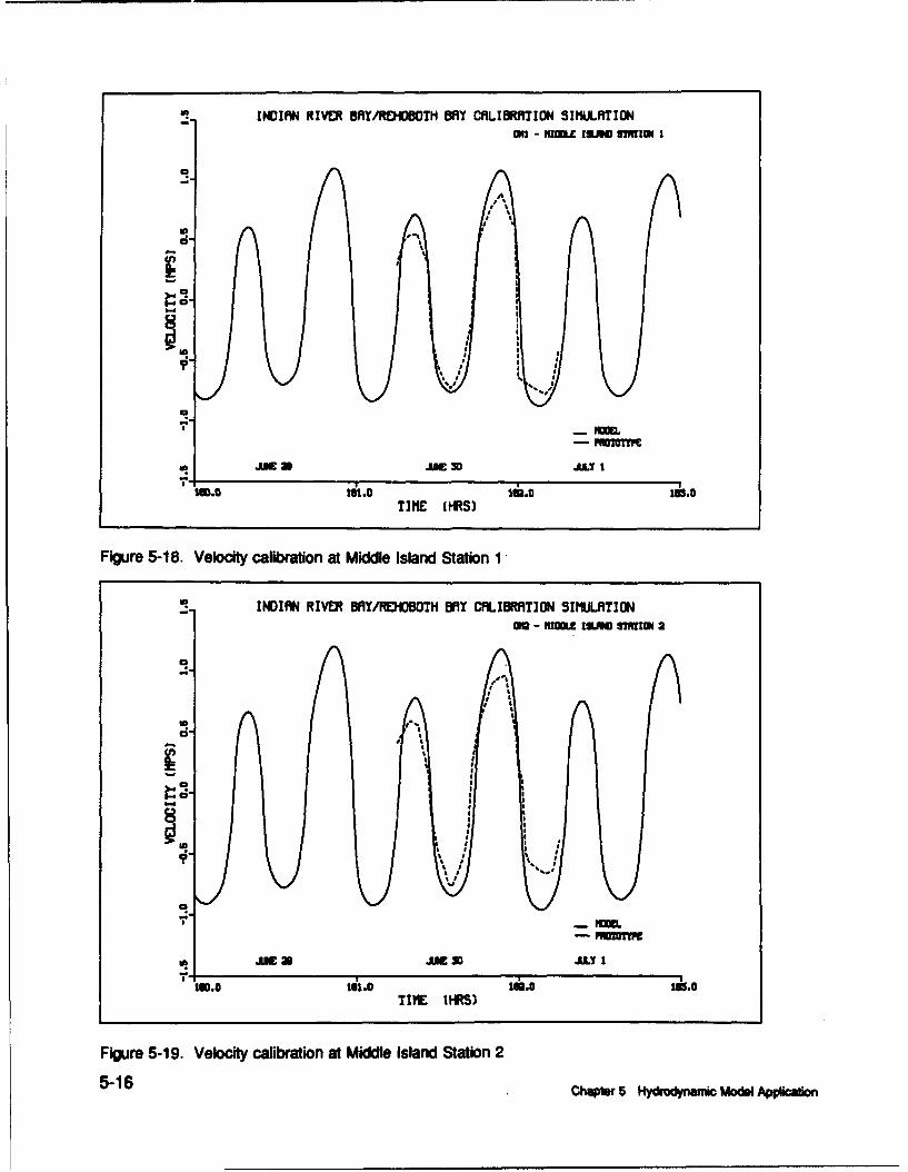
"IINDIflN RIVER BAY/REHOBOTH BRY CFALIBRATION SINULATIONon - NIZL Ixma umlrlnm

0

Li~

U,-

o

J.o n•. lem. m JLYT I M HRS)

Figure 5-18. Velocity calibration at Middle Island Station I

,e. ~INOIRlN RIVER BAY/AEHOBOTH B¥ L'FILIMRfTICN SIMLUITION

aml - N~IMLZ1w I 5,,m m arRIl

iii

0 JA JU a i 0 -LyI

M3.0 131.0 dUJ 10.

T.o. E L.oS)

Figure 5-19. Velocity calibration at Middle Island Station 2

5-16 Chwmr 5 Hydrodyri Model A•iko

.INOIN RIVER BAY/RDIOSOTH DRY CfRLIDRRTION SIIMLT.IONM - KUinZ 1939 SUmN 3

0

a ,.

I ,

a

I.~m

0.0 A2A3.0TIME (IRS)


".IlIRN RIVER BAY/REOOOCH BDRY CALIBRATION SIMULATIONON - NIOMn I9•.8•W 4

ma"

/ :

M UhU0 A2.0 .0

TIME MJRS)


Ctwpbr 5 ym•a ModW Appion 5-17

supplied to the model at a 1-hr interval using a low-low pass filter on therecorded time series. Water levels were linearly interpolated by the model foreach time step between the 1-hr input values and were uniformly assigned toevery cell on the open boundary. No water surface level gradient was imposedalong this boundary.

Wind speed and direction used in the model were recorded by the DelawarePower and Light (DPL) anemometer. Wind data were supplied to the model at1-hr intervals and were linearly interpolated for time steps between the 1-hrinput values.

Discharge data for the validation period were estimated by ratio techniquesdescribed in Chapter 3. River discharge rates for the validation period wereaverage. The Millsboro Dam flow rate was approximately 1.66 m3/sec and theVines Creek flow rate was approximately 0.05 m3/sec. Discharge data wereestimated as daily average flow rates, therefore model input consisted of oneflow rate for each day of the simulation. Flow rates were updated at each timestep of the simulation by linearly interpolating between daily values.

Analysis of Validation Results

As with the calibration period, the model accurately reproduces the ampli-tude of the water surface level time histories recorded at the Vines Creek,Potnets, Massey, and Dewey gauges, however, the model consistently leads theprototype by 30 minutes at all gauges (Figures 5-22 through 5-25). Scatterplots of predicted versus measured water surface levels show the typical ellip-tic shape indicative of a phase shift (Figures 5-26 through 5-29). The imserror at the Vines, Potnets, Massey, and Dewey gauges was computed to be5.1, 4.3, 3.3, and 1.8 cm respectively. Again, the cause of the discrepancy ismost likely due to the boundary condition applied across the inlet boundary.

By adjusting the boundary forcing function 30 minutes, the model resultsare in phase with the prototype data at all four gauges (Figures 5-30 through 5-33). In addition, the scatter plots of predicted versus measured water surfacelevel lose their elliptic shape and show a linear relationship between modelresults and prototype data (Figures 5-34 through 5-37). The mis error at theVines, Potnets, and Massey gauges was reduced to 2.8, 2.0, and 1.3 cm,respectively. The rms error at the Dewey gauge did not change.

Salinity Overview

The salinity distribution in the Indian River Bay-Rehoboth Bay systemvaries both spatially and temporally. Indian River Bay has a strng salinitygradient in the east-west direction, whereas Rehoboth Bay responds fairlyuniformly (Figure 5-38). The strong east-west salinity gradient in Indian RiverBay is clearly the result of saltwater inflow through Indian River Inlet (to the

5-18 Chapter 5 Hydmdynamic Mo Applic••ion

-. fINDI4N RIVER DRY/RD M DAY VmliFCnirO SImuA..IONOC R 14-20, 1988

I• •~T - VS.aat

d-

I sd

OCT 14 OCT15 I Tis OCT 17 AOCT3 OCT 13 OCT 20

14.0 15.0 15.0 1.o 4.0.0 W0.0 21.0TIME (DAYS)

Figure 5-22. Tidal verification at Vines Creek gauge

- INDI1N RIVER DAY/R!UIO80T BAY VeRIFICRTIoN sImULrTION0CT09ER 14-20, 1988

72-PMIlN

ci--

1e 4.0 15.0 4.0 Ii.O ii.o 4•.0 2i.0 'm.0TIME (OilS)

Figure 5-23. Tidal verification at Potnets gauge

Chqps 5 Hy~uynamic Mode Application 5-19

- .. INDIRN RIV!R WfVY/REDO O DRY Va i flCA7IciN s$I urTIONOCTOBER 14-20, 1988

* -'mmIt r4 ots UTI miT oCt3 U113 o01

14.0 15.0 13.0 0.0 .0 13.0 .0 =1.aTIME (ODYS)

Figure 5-24. Tidal verification at Massey's Ditch gauge

- '" INOIRN RIVER BAY/ KF21OM OTH BAY VaItIrIc 'N sIMULATIONOCTOBER 14-20, 1988

r-E-

K C 14 O01 s OCTisO3IT 0013 OOTCT o•00

14.0 1i.0 4.0 1;.0 4.0 14.0 U.o 2i.0TIWE (ORYS)

Figure 5-25. Tidal verification at Dewey Beach gauge

5-20 ChimW 5 Hydrodynaic Mo. ,picapon

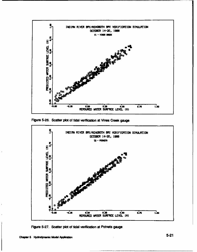
S" IIC14ND RIVER Wft/RUOO DRY VairiCniON SlIUTIONOCTOBER 14-20, 198

TI' - Wil

i,°oout

"OSIMStJ£ WRTCR SUmRFCE LEVEL (M)

Figure 5-26. Scatter plot of tidal verification at Vines Creek gauge

S- JINDIFI RIVER BRY/ROIODOTh ERY VERIFICRTION SIIJLATIONOCTOBER 14-20, 19i8

-a

I,,

1910

-.0 -03n 0.00 0.3 0.00 0.15 1.00ESUE HATR SU C LEVEL (M)

Figure 5-27. Scatter plot of tidal verification at Potnets gauge

chqsr 5 Hyodnam o L40M Appl o 5-21

INDIAN RIVEt DIY/RDCOUTH DAY VOUIICATION 5IIsIJLRIONOCT0UI 14-20, 19O

U3 - WMOl

EZI!-'88

I,

-LU -0.3 0.3 LUW LUW 0.1 1?1DSUAEO MAWER SIRTRCE LEVEL (H)

Figure 5-28. Scatter plot of tidal verification at Massey's Ditch gauge

'8

,.:" INDIANi RIVER DRYRDOOT DRY voRFItirfic simuIFINm• • 14-20, 1900

ci,

J.

-0.3 -0.x 0:3 0.3 0.15O 1.3ISM MATER SUI WE LEVEL (M)

Figure 5-29. Scatter plot of tidal caflbrtlon at Dewey Beach gauge

5-22 Chps 5 Hydrodm mic Mod Apphmi

east) and freshwater inflow from Indian River at Millsboro Dam (to the west)(Karpas 1978). For low flow conditions, freshwater does not penetrate as farinto Indian River as under high flow conditions, resulting in a lower salinity

gradient from the inlet boundary to the river boundary. Conversely, high flowconditions push freshwater far into Indian River, resulting in a higher salinitygradient from the inlet boundary to the river boundary. Comparing high flowconditions during flood and ebb shows the limits of salinity excursion inIndian River Bay are strongly influenced by the tide (time of day). For highriver flow conditions and flood flow, salinity in Indian River is compressed bythe strong river flow opposing the tidal flood flow resulting in a steep salinitygradient in Indian River Bay. Under ebb conditions, the salinity gradient isstill large, but the excursion limits are pushed further east by the strong riverflow and ebbing tide.

Rehoboth Bay has no major source of freshwater. Because of this, Reho-both Bay has a higher salinity concentration than most of Indian River Bay,and Rehoboth Bay responds nearly uniformly to the tidal input of salinity.However, there is a weak east-west gradient as a result of freshwater inflowfrom two major creeks (Love and Herring) on the western shore of RehobothBay (Karpas 1978) (Figure 5-38).

Temporal variability of salinity is a function of tidal oscillation (salt-waterinflow) and variation in freshwater inflow, and the interaction of these twofactors. Figures 5-39 and 5-40 show the time variation of salinity from day260 to day 265 of 1988 (September 16-20) in Indian River and Indian RiverBay (grid cells (9,29) and (30,24), respectively), and Figures 5-41 and 5-42show the time variation of salinity near the center of Rehoboth Bay (grid cells(42,54) and (44,60) respectively).

The time series of salinity in the upper reach of Indian River (Figure 5-39)shows a large variation in salinity with tidal oscillations. Salinity in thisregion ranges from a low of 13.7 ppt to a high a 21.5 ppt with an averagevalue of approximately 17-18 ppt. The important point is that salinity variesnearly 8 ppt during one tidal cycle in the upper reach of Indian River. This iscritical from a modeling standpoint because of the sparseness of salinity datafor comparison to model results and the missing component of "time of day"in the salinity data collection process.

Figure 5-40 shows that the time variation of salinity in Indian River Bayhas less influence from Indian River than the previous location and is thereforemore tidally influenced. Salinity in this region ranges from 29.0 to 31.5 pptwith an average value of approximately 30 ppt. At a distance from the influ-ence of freshwater inflow, the variation in salinity is only 2.5 ppl.

Figure 5-41 shows that salinity in the south-central portion of RehobothBay varies slightly with the tide, having a range of only 1 ppt. Salinity in thisportion of Rehoboth Bay varies between 30.5 and 31.5 ppt. Figure 5-42 showsthat salinity in the north-central portion of Rehoboth Bay is nearly constant

5-23Chapt 5 Hydrodynauic Modal Applicdatun

-'" INDIAN RIVER DRY/RDOMBO Y VERIFICRTION SIIIJLRTIONOCTOBER 14-20, 1988

R1 - YBO &M

rE J

OCT14 OCT15 OCTo1 OCT17 C 1i OCT13 19 20

14.0 15.0 4.0 4.0 •.0 19.0 •.0 1.0TIME (DRYS)

Figure 5-30. Tidal verification at Vines Creek gauge

INDIAN RIVER BRY/RDMOBOTH DRY VERIFICRTION SIIIJtUTIONOCT 14-20, 1988

Emm

* -..

its4 O o1 to OCT17 O OCT 1 s CT20

14.0 4.0 15.0 •.0 •.0 4.0 30.0 2'.oTIME (DRYS)

Figure 5-31. Tidal verification at Potnets gauge

5-24 chapW 5 HydrodMknMC ModeM Appicaon

-. It4)IRN RIVER DRY/RDOWTH DRY VERIFICRTION SIJLM.RTIONOCTOER 14-20, 1986

le 73 - NNW

mmm

1OCT4 OCT1i5 OCT1i OLCT17 0013 0a0m OCT

14.0 4a.0 i i. 4. i0 20TIME WOAYS)

Figure 5-32. Tidal verification at Massey's Ditch gauge

INDIRNl RIVER ORY/RDIO8OTH ORY VERIFICRTION SIIIJLATIONOCTOBER 14-20, 1988

J,;

- rUTOMU

0 C14 OCT OCT OCT1 CT17 OCT is OT1i OCT14.0 1.o 4.0 1.0 A.0 4.o .o.

TIME (DRYS)

Figure 5-33. Tidal verification at Dewey Beach gauge

chq s 5 Hyodynamic Mod po• cn 5-25

110111 RIVE~ WYAMOWTM MY VI~tITICATION SIPIJLTIONOCxE 14-20, 196

-m -0.35 0.0 0a3 0.3 0.5 1.00?ERSURE NlIMiR SURFFCE LEVEL MII

Figure 5-34. Scatter plot of tidal verification at Vines Creek gauge

- 1101114w RIVER MY/EHww h fAY vEtriIcATi0N simmIIioNOCTOERM 14-20, 1966

Fit

-. - 0.3 0.30 0. 0.30 05 1.MNUMM~ WRIMER SURFACE LEVEL (M11

Figure 5-35. Scatter plot of tidal verification at Potnets gauge

5-26 cewpwsr5 Hy~dronamic Monl Applicln

INDIIN RIVER DRY/RDODOh DRY VERI[IcnoN siIlATIrONOCTOBR 14-20, 1988

13-oIU!Z~

153

-o

J,

-0.3 -0.=3m ~ 0:13030. 0,75 1.3MERSM M SUNW , ILVE.L (I)

Figure 5-36. Scatter plot of tidal verification at Massey's Ditch gauge

INDIRI RIVER 51Y/RODt0 DRY VERIFICRTION SIMJAUTIONOCTOBER 14-20, 1968

T4 - MY

-;

pita.

,-o.m -Ka Z= 03 o.,, I=HERSURi WHTER SURFME LEVL (11)

Figure 5-37. Scatter plot of tidal caibration at Dewey Beach gauge

Chapar 5 Hymdynmmic Mod AppcaiUon 5-27

*29 < S

M26 < S < 29

FO23 < S < 26i20 < S < 23

17 <S <20

Figure 5-38. Indian River Bay/Rehoboth Bay salinity distribution

with time (31.2 ppt). Rehoboth Bay has no major freshwater inflows and istherefore tidally-dominated.

In conclusion, Indian River Bay is the more complex of the two bays inthis system from a salinity standpoint. Salinity varies both spatially and tem-porally in Indian River Bay due to the interaction of salt water from the inletand freshwater from Indian River at MillsY - Dam. Rehoboth Bay is nearlyhomogeneous. There is no major source oi freshwater inflow to Rehoboth Bayand it is therefore clearly tidally-dominated.

Salinity Calibration and Validation

A long-term (1 year) simulation was used in the salinity calibration. Themodel simulation period was year 1988, however prototype data available forthis time period was limited to 3 days of spatially-distributed salinity. A time-series of salinity at one location would therefore be limited to 3 values for the

5-28 Chapter 5 Hydrodynamic Model Application

IN0I1N RIVER my ONC-YEC SIHIrRTION

-!TIME (DRlYS)

Figure 5-39. Temporal variation of salinity in Indian River

am I lAl 130,N

9

c.

x"

TRIEC (ORYS)

Figure 5-40. Temporal variation of salinity in Indian River Bay

Ch@PW 5 Hydrodynamic Model Al~ikMoM 5-29

INOIfRd RIVER ORY OIC-YECAR SIIIULRTION

20.0 a1.0 SkA 2.0 204.0 2.0TINC (ORYS)

Figure 5-41. Temporal variation of salinity in Rehoboth Bay (42,54)

IND119N RIVER ORY UlC-YEFI SIMAITION

X,

TIME 11ATS)

Figure 5-42. Temporal variation of salinity in Rehoboth Bay (44,60)

5-30 Chapter 5 Hydrodynamic Model Application

entire year. Thus, a spatial comparison of model results to prototype data wasused. These data provide a picture of the spatial distribution of salinity at14 stations for June 20, July 25 and September 19, 1988. As previously dis-cussed, it is important to note that the exact time of day for data collection isnot available. This factor is most critical in Indian River where the temporalvariation of salinity can be as much as 8 ppt during one tidal cycle.

For illustration, Figure 5-43 is a model predicted salinity snapshot of theentire study area at 12 noon on September 19, 1988 with the shaded circlesindicating measured salinity values. Note that measured salinity values aresingle, "instantaneous" values, however the time of day that the data werecollected is not known. For this reason, model results were arbitrarily saved at12 noon. (This is critical in areas where the temporal variability of salinity issignificant.) Results in Rehoboth Bay are excellent. Results in Indian RiverBay are very good, with the exception of the upper reach of Indian Riverwhere the model is underpredicting salinity. The model salinity saved for thisregion is in the range 14-17 ppt, however, the prototype value is in the 17-20 ppt range.

Reviewing the time-series' of salinity for the central portion of RehobothBay (Figure 5-41 and 5-42) shows that salinity is nearly constant, therefore thetime of day for data collection is not critical. In contrast, the time-series ofsalinity in the upper reach of Indian River (Figure 5-39) shows great variabilityin salinity with tide (time of day). Thus, the difference between model resultsand prototype data in Indian River is well within the range of temporal vari-ability of salinity for this region.

Although the model results are within the range of temporal variability,salinity values in Indian River are consistently lower than the prototype valuesfor all three days of data collection in 1988. Therefore, several techniqueswere examined to obtain a better salinity calibration in the upper reach ofIndian River. The technique selected was to increase the size of a few cells inthe upper reach of Indian River. The added cell volume decreased the velocityof freshwater inflow thereby allowing salt to penetrate further into IndianRiver. In addition, a spatially-variable dispersion coefficient was used to cali-brate the model. A value of 12 m2/sec was used in Rehoboth Bay and most ofIndian River Bay with the exception of a portion of the middle reach of IndianRiver (cells 4-14). A spatially variable longitudinal dispersion coefficient wasused to calibrate the model to the high salinity gradient observed in this regionin 1988, 1989, and 1990. This section of the Indian River is a shallow chan-nel where freshwater from the river meets salt water from the lower estuary inaddition to heated water discharged from the DPL power plant. Smith (1976)reported that in the presence of buoyant concentration either from a river orfrom heated water, the transverse circulation can lead to a marked reduction inlongitudinal dispersion. It is believed that this occurred in the central portionof Indian River. For this reason, a smaller dispersion value of 0.6 m2/sec wasused in cells 7 through II and was gradually increased to 12 m2/sec in boththe upstream and downstream directions. The desired salinity distribution wasthus obtained.

Chapter 5 Hydrodynamic Model P"olication 5-31

20 <S3<23

17 < S3( 2014 < S< 17rS S<14

Figure 5-43. Salinity calibration for September 19, 1988

A second long-term (1-year) simulation was used in the salinity validation.The model simulation period was year 1989, however prototype data availablefor this time period was limited to 2 days of spatially-distributed salinity. Atime-series of salinity at one location would therefore be limited to 2 valuesfor the entire year. Thus, a spatial comparison of model results to prototypedata was again used. These data provide a picture of the spatial distribution ofsalinity at 14 stations for April 24 and October 17, 1989. Figure 5-44, depict-ing the April 24, 1989 model-prototype comparison, is during a period of highflow from Indian River. The results are excellent with the exception of onelocation in Rehoboth Bay. At gage 5, the prototype data indicates a highersalinity (>29 ppt) than the model predicts (26-29 ppt). However, the actualsalinity value is only 29.9 ppt and the discrepancy is therefore small. Thelower value of model salinity indicates that the salinity wedge should be forcedfurther into Rehoboth Bay. Figure 5-45, depicting the October 17, 1989model-prototype comparison, is during a period of low flow from Indian River.Model results are excellent at all gages.

5-32 ChapWr 5 Hydrodynamic Model Aplaton

2 <s S=26 < S < 29

23 < S < 26

17 < S < 20

14 S< 1 S <" 17

Figure 5-44. Salinity validation for April 24, 1989

Summer Average Salinity

The link between hydrodynamic and water quality modeling is in the con-servative property of salinity. In water quality modeling, summer is thechemically- and biologically-active time period. Therefore, a comparison ofdata and model results in the summer months is important to ensure the accu-racy of concentration transport. Since the data available in the summer monthsprecludes a time series comparison, the average summer conditions weremodeled and compared to all measured data for the summers of 1988, 1989,and 1990. Summer was defined in the model as July, August, and September.Figures 5-46 through 5-48 show comparisons between model and prototypedata for the summers of 1988, 1989, and 1990, respectively. The three-monthaverage of model salinity from the head of the Indian River (Millsboro Pond)to Indian River Inlet is given as a solid line and prototype data at 8 salinitystations on three specific days each year (July 24, 1989, August 28, 1989,September 25, 1989; July 16, 1990, August 13, 1990, September 24, 1990) aregiven as +'s. In 1988 only two days of salinity data (July 25, September 19)were available. The results confirm that the summer trend for salinity is

Chapter 5 Hydrodynamic Model Application 5-33

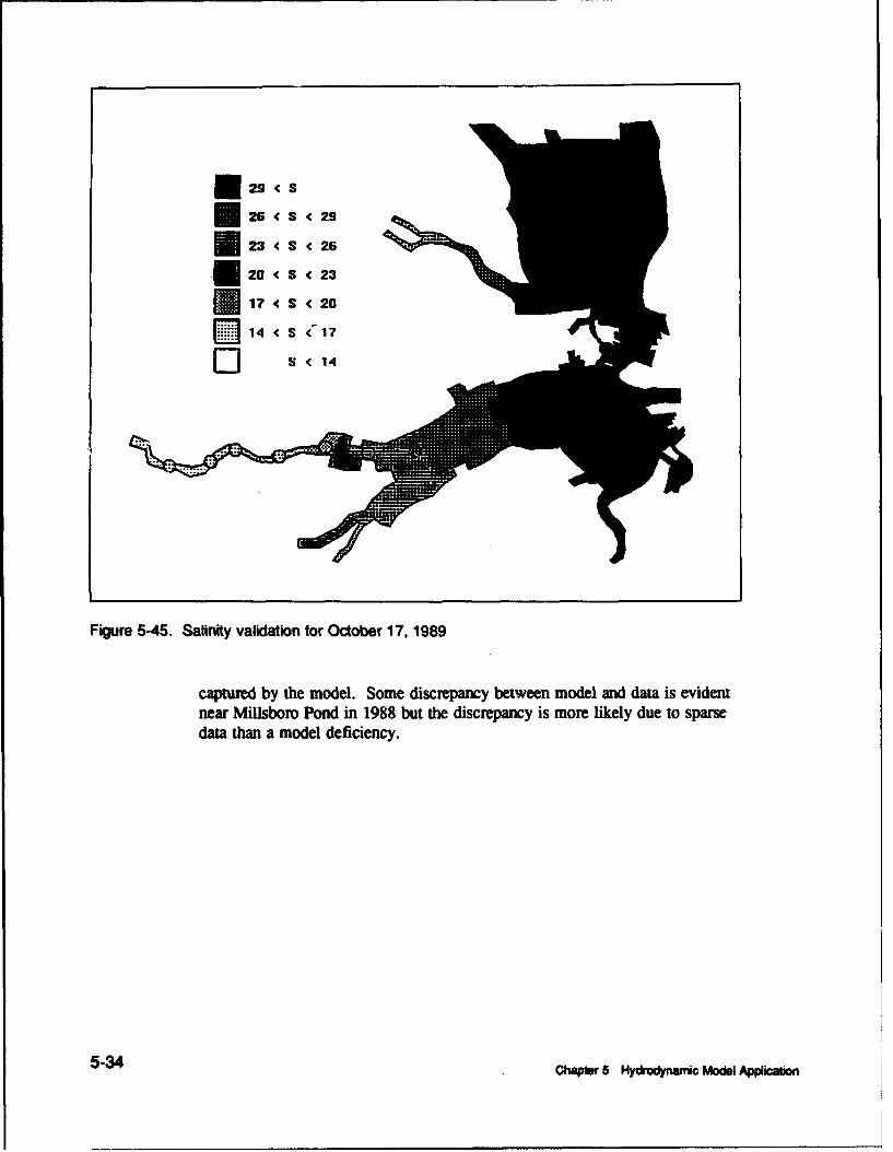
i20 < S < 23

Figure 5-45. Salinity validation for October 17, 1989

captured by the model. Some discrepancy between model and data is evidentnear Millsbor Pond in 1988 but the discrepancy is more likely due to sparsedata than a model deficiency.

5-34 hapte.r 5 Hydrodynamic Model App• ation

INDIRN RIVER BAY SRLINITY DISTRIBUTIONWIER 1988

30-

+- +

S15- +

10- PROTOTYPE DATA

+- - II�OEL RESULTS

5-

MILLSBORO PONO INDIAN RIVER INLET

; 14 isDISTIA ALONG INDIAN RIVER BAY (KILOMETERS)

Figure 5-46. Indian River Bay salinity distribution, Summer 1988

INDIAN RIVER BFY SRLINITY DISTRIBUTIONSUMMER 1989

3o-I

-I.

10+

15

s-4~ + PROTOTYPE M~~f5 -

Z m m m .

0 2

DISTLNCE ALONG INDIRN RIVER BRY (KILOMETERS)

Figure 5-47. Indian River Bay salinity distribution, Summer 1989

Chlmr 5 H ModW Appkwn 5-35

INDIRN RIVER BRY SFLINITY DISTRIBUTIONSUMMIER 1990 4

30-

+

1o- + PROTOTYPE DRTH4.

- MOEL RESULTS

MILLSBORO POND INDIRN RIVER INLETO0 V2 10 "" 1

DISTFNCE ALON INDIAN RIVER BAY (KILOMETERSI

Figure 5-48. Indian River Bay saliniy distrbution, Summer 1990

5-36 ChwWmr 5 Hydwnk Mod App•ic•on

Chapter VI: Water QualityModel Kinetics

Introduction

The water quality model, dubbed CE-QUAL-ICM, onginated as part of aeutrophication model package applied to Chesapeake Bay (Cerco and Cole1993). Kinetic formulations from the Chesapeake Bay model were applied toIndian River-Rehoboth Bay with minimal modification. Several state variablespresent in the original model were dropped, however, consistent with the avail-able data base. Some simplifications were also made, largely through specifi-cation of parameter values. The original code is intact and additional statevariables and options can be activated in the future. Active state variables inIndian River-Rehoboth Bay are presented in Table 6-1. The remainder of thechapter describes the state variables, details kinetics formulations, and listscoefficient values.

Table 6-1Water Quality Model State Variables

Temperatune Salinity

MAeo Dissolved Organic Carbon

Labile Parliculate Organic Carbon Reftracitoy Particulate Organic Carbon

Ammonium Nilrefe

Dissolved Organic Nitrogen Labile Parliculate Organic Nitrogen

Refractory Particulate Organic Nitrogen Total Phosphate

Dissolved Organic Phosphorus Labile Partikulae Organic Phosphorus

Refractory Particulate Organic Phosphorus Dissolved Oxygen

Algae

Algae are a primary focus of the eutrophication model. Algae play a cen-tral role in the carbon, nitrogen and phosphorus cycles. Dissolved oxygen isinfluenced by algal production and respiration in the water column. Light

Cetpter 6 owaui aij~y MoM M6-1

extinction is partially dependent attenuation caused by algal chlorophyll. Onealgal group is currently activated in the model.

Organic Carbon

Three organic carbon state variables are considered: dissolved, labile partic-ulate, and refractory particulate. Labile and refractory distinctions are basedupon the time scale of decomposition. Labile organic carbon decomposes on atime scale of days to weeks while refractory organic carbon requires moretime. Labile organic carbon decomposes rapidly in the water column or thesediments. Refractory organic carbon decomposes slowly, primarily in thesediments, and may contribute to sediment oxygen demand years afterdeposition.

Nitrogen

Nitrogen is first divided into organic and mineral fractions. Organic nitro-gen state variables are: dissolved organic nitrogen, labile particulate organicnitrogen, and refractory particulate organic nitrogen. Two mineral nitrogenforms are considered: ammonium and nitrate. Both are utilized to fulfill algalnutrient requirements although ammonium is preferred from thermodynamicconsiderations. The primary reason for distinguishing the two is that ammon-ium is oxidized by nitrifying bacteria into nitrate. This oxidation can be asignificant sink of oxygen in the water column and sediments. An intermedi-ate in the complete oxidation of ammonium, nitrite, also exists. Nitrite con-centrations are usually much less than nitrate and for modeling purposes nitriteis combined with nitrate. Hence the nitrate state variable actually representsthe sum of nitrate plus nitrite.

Phosphorus

As with carbon and nitrogen, organic phosphorus is considered in threestates: dissolved, labile particulate, and refractory particulate. Only a singlemineral form, total phosphate, is considered. Total phosphate exists in twostates within the model ecosystem: dissolved phosphate and phosphate incorpo-rated in algal cells. Equilibrium partition coefficients distribute the totalamong two states.

Dissolved Oxygen

Dissolved oxygen is required for the existence of higher life forms. Oxygenavailability determines the distribution of organisms and the flows of energyand nutrients in an ecosystem. Dissolved oxygen is a central component of thewater quality model.

6-2 Ch*r 6 waer Qamy Moa Wneb

Salinity

Salinity is a conservative tracer that provides verification of the transportcomponent of the model and facilitates examination of conservation of mass.Salinity also influences the dissolved oxygen saturation concentration.

Temperature

Temperature is a primary determinant of the rate of biochemical reactions.Reaction rates increase as a function of temperature although extreme tempera-tures result in the mortality of organisms.

Conservation Of Mass Equation

The foundation of CE-QUAL-ICM is the solution of the mass-conservationequation for a control volume. Control volumes in the water quality modelcorrespond to one or more cells on the hydrodynamic model grid. For theIndian River-Rehoboth Bay application, a two-dimensional, vertically inte-grated form of the mass-conservation equation is employed. CE-QUAL-ICMsolves, for each volume and for each state variable, the conservation of massequation:

8ViCi = n (6-1)E = Qj Cj EAj rj + ESi(-1F j1 j=1 j

Vi = volume of ith control volume (M3)

Ci = concentration in ith control volume (gin mi3 )

Qj = volumetric flow across flow face j of ith control volume (M3 sec"1)

Cj* = concentration in flow across flow face j (gin m-3)

AN = area of flow face j (m2)

Dj = diffusion coefficient at flow face j (m 2 sec"1)

n = number of flow faces attached to ith control volume

Si = external loads and kinetic sources and sinks in ith control volume(gin sec"1)

t, x = temporal and spatial coordinates

Chapter 6 Water Quality Model Kimetics 6-3

Solution to the mass-conservation equation is via the finite-differencemethod using the QUICKEST algorithm (Leonard 1979).

The remainder of this chapter details the kinetics portion of the mass-conservation equation for each state variable. Terms are defined where theyfirst appear. Coefficient values are presented in a table at the end of the chap-ter. For consistency with reported rate coefficients, kinetics are detailed usinga temporal dimension of days. Within the CE-QUAL-ICM code, kineticssources and sinks are converted to a dimension of seconds beforL employmentin the mass-conservation equation.

Algae

Sources and sinks of algae are:

Growth (production)Basal metabolismPredationSettling

The governing equation for algal biomass is:

8B=( -BM -PR - ±Sa B (6-2)

B = algal biomass, expressed as carbon (gin C m3 )

P = production (day 1 )

BM = basal metabolism (day-)

PR = predation (day-1)

WSa = algal settling velocity (m day')

H = depth of water column (in)

Production

Production by phytoplankton is determined by the availability of nutrients,by the intensity of light, and by the ambient temperature. The effects of eachare considered to be multiplicative:

6-4 Chapter 6 Water aQuay Model Khetc

P = PM f(N) f(Q) f(T) (6-3)

PM = production under optimal conditions (day 1 )

f(N) = effect of suboptimal nutrient concentration (0 < f < 1)

f(I) = effect of suboptimal illumination (0<$ f < 1)

fmT) = effect of suboptimal temperature (0 < f< 1)

Nutrienit

Carbon, nitrogen, phosphorus, and silica are the primary nutrients requiredfor algal growth. Inorganic carbon is usually available in excess and is notconsidered. Silica is omitted since this nutrient is required only by diatomswhich are not distinguished from other algae in the model application. Theeffects of nitrogen and phosphorus on growth are described by the formulationcommonly referred to as "Monod kinetics" (Monod 1949). In the Monodformulation (Figure 6-1) growth is dependent upon nutrient availability at lownutrient concentrations but is independent of nutrients at high concentrations.A key parameter in the formulation is the "half-saturation concentration".Growth rate is half the maximum when available nutrient concentration equalsthe half-saturation concentration. Liebig's "law of the minimum" (Odum1971) indicates growth is determined by the nutrient in least supply:

f(N) = minimum NH4 + NO3 PO4d (6-4)minmumKiln + NH4 + NO3' KHp + PO4d

NH4 = ammonium concentration (gin N m3)

NO3 = nitrate concentration (gm N m3 )

KHn = half-saturation constant for nitrogen uptake (gin N m-3 )

PO4d = dissolved phosphate concentration (gin P m 3)

KHp = half-saturation constant for phosphorus uptake (gin P m 3)

Ught

Algal production increases as a function of light intensity until an optimalintensity is reached. Beyond the optimal intensity, production declines as

Op 8 W .Qouality Model Knetic 6-5

1

0.9

0.8

0.7

0.6

90.5 f 0.5 When N K-

0.4

0.3

0.2

0.1

0

0 1 2 3 4 5 6 7 8 9 10 11 12 13 14 15

N/KH

Figure 6-1. The Monod formulation for nutrient-limited growth

intensity increases. Steele's equation (DiToro et al. 1971) describes thisphenomenon:

f()=-- e1 R =Ie (6-5)Is

I = illumination rate (Langleys day 1)

Is = optimal illumination (Langleys day-1 )

Steele's equation describes the instantaneous light limitation at a point inspace. The model, however, computes processes integrated over discrete timeintervals and aggregated spatially into model segments. Therefore, Steele'sequation must be integrated over an appropriate time interval and averagedover the thickness of each model segment. The integration interval selected isone day. This interval does not preclude computation steps less than a day butfrees the model from accounting for illumination in "real time." Daily averag-ing does preclude computation of diurnal fluctations in algal production. Thisrestriction is not severe, however, since the classic equations for algal growthare not appropriate for short time scales.

6-6 ChGs 6 Waha y Modmi KII Uw

Assuming light intensity declines exponentially with depth, the integrated,averaged form of Steele's equation is:

2.72 FD (eab - eat) (6-6)

Keo -Hes

lb = - e -Ken H (6-7)FD Is

Ot= 10 (6-8)FDIs

Io = daily illumination at water surface (Langleys day 1)

HD = fractional daylength (0 _ FD < 1)

Kess = total light attenuation coefficient (rn-)

Light attenuation in the water column is composed of two fractions: a back-ground value dependent on water color and concentration of suspended parti-cles, and extinction due to light absorption by ambient chlorophyll:

Kess = Keb + KechlB (6-9)CChl

Keb = background light attenuation (rn-)

Kechl = light attenuation coefficient for chlorophyll 'a' (m2 mg"1 )

CChl = algal carbon-to-chlorophyll ratio (gin C mg"1 chl)

Optimal illumination for photosynthesis depends on algal taxonomy, dura-tion of exposure, temperature, nutritional status, and previous acclimation.Variations in optimal illumination are largely due to adaptations by algaeintended to maximize production in a variable environment. Steele (1962)noted the result of adaptations is that optimal illumination is a consistent frac-tion (- 50%) of daily illumination. Kremer and Nixon (1978) reported ananalogous finding that maximum algal production occus at a constant depth(- lm) in the water column. Their approach is adopted here so that optimalillumination is expressed:

6-7ch@ts6 WMs0QalitM RMo Kinti

Is = loavg e" Ken Dopt (6-10)

loavg = adjusted surface illumination (Langleys day-1)

Dopt = depth of maximum algal production (m)

A minimum, Ismin, is specified for optimal illumination so that algae donot thrive at extremely low light levels. The time required for algae to adaptto changes in illumination is recognized by computing Is based on a time-weighted average of daily illumination:

Ioavg = 0.7 Io + 0.2 11 + 0.1I2 (6-11)

II = daily illumination one day preceding model day (Langleys day-)

12 = daily illumination two days preceding model day (Langleys day-')

Four independent parameters influence the effect of light on algal produc-tion: FD, Ke, Dopt, and H. The parameters Ke and Dopt, and Ke and H occuras products, however, so the number of independent parameters that determinethe light effect is actually three: FD, Ke * Dopt, and Ke * H.

Fractional daylength, FD, occurs as a multiplier and in the exponentialterms of the integrated form of Steele's equation (Equation 6-6). The neteffect of FD on the light function is nearly linear, however (Figure 6-2). Atthe latitude of Indian River, FD is limited to the range '0.4 to 0.6 so that f(I)varies by -50% from the shortest to longest day of the year.

A plot of the effects on growth of the pairs Ke * H and Ke * Dopt (Fig-ure 6-3) has numerous interpretations. For Ke * H >> Ke * Dopt, growthdiminishes as Ke * H increases. In other words, growth goes down as lightextinction and/or depth increase. For much of the feasible range of Ke * H,growth is only weakly dependent on Dopt Thiis weak dependence was onefactor in the selection of the light-effect formulation. Maximum growth occurswhen Ke * H is slightly larger than Ke * Dopt (when H is slightly larger thanDopt). When Ke * H < Ke * Dopt (H _ Dopt), growth is diminished frmn themaximum due to light levels in the majority of the water column occupyingthe supersaturated range for algal growth. For small Ke * H (shallow systemswith little light attenuation) maximum growth occurs when Dopt = 0. WhenDopt = 0, no portion of the water column is in the supersauted ringe. Formuch of the feasible range of Ke * H, however, maximum production occurswhen Dopt > 0. For this case, diminished production due to light supemtura-ton near the surface is offset by increased production at deeper depths.

6-8 ChotWr 6 WMuW O tI MOM Khef

0.45Ke = 0.7 / meter

0.4 H-Smeter

0.35Dopt -1 meter

0.3

0.25

S0.2

0.15

0.1

0.05

0 I

0 0.1 0.2 0.3 0.4 0.5 0.6 0.7 0.8 0.9 1

FD

Figure 6-2. Effect of fractional daylength on algal light limitation

0.50.45. Dopt * Ke = 0.0

0.4 - , Dept* Ke-0.50.35 - -•

0 .2.-" .......... Dopt*Ke 1.0

0.2 .0.1 :/0.1

0.05 I

0 I I

0 5 10 15 20 25

Ke*H

Figure 6-3. Effect of light extinction, total depth, and optimal depth on algal ight limhitation

ChW e 6waw Ouft od I I rief 6-9

Temperature

Algal production increases as a function of temperature until an optimumtemperature or temperature range is reached. Above the optimum, productiondeclines until a temperature lethal to the organisms is attained. Numerousfunctional representations of temperature effects are available. Inspection ofgrowth versus temperature curves indicates a function similar to a Gaussianprobability curve (Figure 6-4) provides a good fit to observations:

f(T) = e- KTgl (T - Tm)2 when T5Tm (6-12)

= e - KT2 (Tim - T)2 when T > Tin

T = temperature (C0)

Tm = optimal temperature for algal growth (CO)

KTg1 = effect of temperature below Tm on growth (C, -2)

KTg2 = effect of temperature above Tm on growth (CO-2)

KTgl - 0.0040.9

KTg2 -0.0060.S Tm 200.70.6

90.5 -

0.40.30.20.1

0 I I I I

0 5 10 15 20 25 30DEGREES C

Figure 6.4. Effect of temperature on algal production

6-10 Chapr S Wa m"Od Modm Kd

Basal Metabolism

As employed here, basal metabolism is the sum of all internal processesthat decrease algal biomass. A portion of metabolism is respiration which maybe viewed as a reversal of production. In respiration, carbon and nutrients arereturned to the environment accompanied by the consumption of dissolvedoxygen. A second internal sink of biomass is the excretion of dissolvedorganic carbon.

Respiration cannot proceed in the absence of oxygen. Basal metabolismcannot decrease in proportion to oxygen availability, however, or algae wouldapproach immortality under anoxic conditions. To solve this dilemma, basalmetabolism is considered to be independent of dissolved oxygen concentrationbut the distribution of metabolism between respiration and excretion is oxygen-dependent. When oxygen is freely available, respiration is a large fraction ofthe total. When oxygen is restricted, excretion becomes dominant. Formula-tion of this process is detailed in the text that describes algal effects on carbonand dissolved oxygen.

Basal metabolism is commonly considered to be an exponentially increasing(Figure 6-5) function of temperature:

BM = BMreKTCIT - Tr) (6-13)

BMr = metabolic rate at Tr (day"1)

KTb = effect of temperature on metabolism (CO -1)

Tr = reference temperature for metabolism (CO)

Predation

Detailed specification of predation rate requires predictive modeling ofzooplankton biomass and activity. At present, zooplankton are not included inthe model. Consequently, a constant predation rate is specified. This specifi-cation implicitly assumes zooplankton biomass is a constant fraction of algalbiomass. Zooplankton activity is assumed to be influenced by temperature andis taken into account by incorporating an exponential temperature relationship(Figure 6-5) into the predation term. The predation formulation is identical tobasal metabolism. The difference in predation and basal metabolism lies in thedistribution of the end products of these processes.

PR = BPReKThtT - Tr) (6-14)

BPR = predation rate at Tr (dayt )

Chaplar 6 Waer oudy Mode KnMe 6-11

KT 0.069 / degree C 21.8

1.6

1.41.2

0.8

0.40.2

-10 -7.5 -5 -2.5 0 2.5 5 7.5 10

T - Tref

Figure 6-5. Exponential terrperature function

Effect of Algae on Organic Carbon

During production and respiration, algae primarily take up and producecarbon dioxide, an inorganic form not considered in the model. A small frac-tion of basal metabolism is exuded as dissolved organic carbon, however, andin the model this fraction increases as dissolved oxygen becomes scarce.Algae also produce organic carbon through the effects of predation. Zooplak-ton take up and redistribute algal carbon through grazing, assimilation. respira-tion, and excretion. Since zooplanklon are not included in the model, routingof algal carbon through zooplankton is simulated by empirical distributioncoefficients. The effects of algae on organic carbon are expressed:

.DOC-

(6-15)

((Fa) + (I - FCD) K ~ BEM + FCDPPRJB

.LPOC FCLP PR B (6-16)

6-12 QWpb 6 WAI Ouak ModW Mnkw

RPOC = FCRPPRB (6-17)

DOC = dissolved organic carbon concentration (gmi C m"3)

DO = dissolved oxygen concentration (gin 02 m-3)

LPOC = labile particulate organic carbon concentration (gmn C m-3)

RPOC = refractory particulate organic carbon concentration (gmi C m-3)

FCD = fraction of basal metabolism exuded as dissolved organic carbon

KHr = half-saturation concentration for algal dissolved organic carbonexcretion (gin 02 m-3)

FCDP = fraction of dissolved organic carbon produced by predation

FC.P = fraction of labile particulate carbon produced by predation

FCRP = fraction of refractory particulate carbon produced by predation

The sum of the three predation fractions must equal unity.

Effet of Algae on Phosphorus

Algae take up dissolved phosphate during production and release dissolvedphosphate and organic phosphorus through mortality. As with carbon. the fateof algal phosphorus released by metabolism and predation is represented bydistribution coefficients. Since the total phosphate state variable includes bothintra and extracelular phosphate, no explicit ron of the effect ofalgae on phosphate is necessary. Distribution of total phosphate is determinedby partition coefficients as detailed in the '?HOSPHORUS" section of thischapter. The equations that express the effects of algae on organic phosphorusare:

.•DOP = (BMFPD + PRFPDP) APCB (6-18)

.LPOP (BM FPL + PRFPLP)APCB (6-19)

chir 6 Wair Qudy Mode KWt 6-13

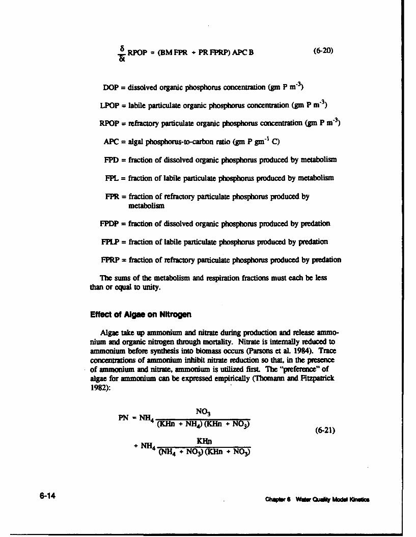
RPOP = (BM FPR + PR FPRP) APC B (6-20)

DOP = dissolved organic phosphorus concentration (gm P m"n)

LPOP = labile particulate organic phosphorus concentration (gin P m"3)

RPOP = refractory particulate organic phosphorus concentration (gin P m"3)

APC = algal phosphorus-to-carbon ratio (gin P gm"1 C)

FPD = fraction of dissolved organic phosphorus produced by metabolism

FPL = fraction of labile particulate phosphorus produced by metabolism

FPR = fraction of refractory particulate phosphorus produced bymetabolism

FPDP = fraction of dissolved organic phosphorus produced by predation

FPLP = fraction of labile particulate phosphorus produced by predation

FPRP = fraction of refractory particulate phosphorus produced by predation

The sums of the metabolism and respiration fractions must each be lessthan or equal to unity.

Effect of Algae on Nitrogen

Algae take up ammonium and nitrate during production and release ammo-nium and organic nitrogen through mortality. Nitrate is internally reduced toammonium before synthesis into biomass occurs (Parsons et aL 1984). Traceconcentrations of ammonium inhibit nitrate reduction so that, in the presenceof ammonium and nitrate, ammonium is utilized first. The "preference" ofalgae for ammonium can be expressed empirically (Thomann and Fitzpatrick1982):

PN=-H 4 = NN11 NO)+NH4 ) (Kn +N(6-21)

+ NH4KHn

(NH4 + NO3) (KHn + NO3)

6-14 cmw 6 WSe Gus* Madi *me=

PN = algal preference for ammonium uptake (0 < PN < 1)

The ammonium preference function (Figure 6-6) has two limiting values.When nitrate is absent, the preference for ammonium is unity. When ammo-nium is absent, the preference is zero. In the presence of ammonium andnitrate, the preference depends on the abundance of both forms relative to thehalf-saturation constant for nitrogen uptake. When both ammonium and nitrateare abundant, the preference for ammonium approaches unity. When ammo-nium is scarce but nitrate is abundant, the preference decreases in magnitudeand a significant fraction of algal nitrogen requirement comes from nitrate.

0.9

NH41KH-0.5

0 .7 ,\ ,......... NH4 KH- 12.0

0......................................................HIHW.NH41KIH-5.0

0.3S10.4--...... -- NH41IKH=-10.

0.2

0.1 KH 0.01 sm N /m0'

0 I i

0 I 2 3 4 5 6 7 a 9 10

N03 I KH

Figure 6-6. Ammonium preference function

The fate of algal nitrogen released by metabolism and predation is repre-sented by distribution coefficients. The effects of algae on the nitrogen statevariables are expressed:

NH 4 = (BM FNI + PR FNIP - PN P) ANC B (6-22)

C~h~wr 6 Water Qualiy Mode Kiti 6-15

.NO 3 = (PN - 1)PANCB (6-23)

DON = (BM FND + PR FNDP) ANC B (6-24)

tLPON = (BM FNL + PR FNLP) ANC B (6-25)

RPON = (BM FNR + PR FNRP) ANC B (6-26)

DON = dissolved organic nitrogen concentration (gin N m-3)

LPON = labile particulate organic nitrogen concentration (gin N m-3)

RPON = refractory particulate organic nitrogen concentration (gin N m-3)

ANC = algal nitrogen-to-carbon ratio (gin N gm"1 C)

FNI = fraction of inorganic nitrogen produced by metabolism

FND = fraction of dissolved organic nitrogen produced by metabolism

FNL = fraction of labile particulate nitrogen produced by metabolism

FNR = fraction of refractory particulate nitrogen produced by metabolism

FNIP = fraction of inorganic nitrogen produced by predation

FNDP = fraction of dissolved organic nitrogen produced by predation

FNLP = fraction of labile particulate nitrogen produced by predation

FNRP = fraction of refractory particulate nitrogen produced by predation

The sums of the metabolism fractions and the predation fractions must eachequal unity.

6-16 ChWn B WMu Out MO *KMOM

Algal Stolchlometry

Algal biomass is quantified in units of carbon. In order to express theeffects of algae on nitrogen and phosphorus, the ratios of nitrogen-to-carbon

and phosphorus-to-carbon in algal biomass must be specified. Global mean

values of these ratios are well known (Redfield et al. 1966). Algal composi-

tion varies, however, especially as a function of nutrient availability. As nitro-

gen and phosphorus become scarce, algae adjust their composition so that

smaller quantities of these vital nutrients are required to produce carbonaceous

biomass (Droop 1973; DiToro 1980; Parsons et al. 1984).

Observations from upper Chesapeake Bay were examined to assess the

potential variability of algal stoichiometry (Cerco and Cole 1993). The varia-

tion of carbon-to-nitrogen stoichiometry in the upper Bay was small. As a

consequence of these observations, the model formulation specified constant

algal nitrogen-to-carbon ratio, ANC. Large variations in carbon-to-phosphorusratio occurred, however. To account for this effect, a variable algal phospho-rus-to-carboni ratio, APC, was formulated in the model. Variable stoichiometrywas not employed in the Indian River-Rehoboth Bay application. The formu-

lation that allowed variable APC required distinctive treatment of the phos-

phate state variable, however.

Effect of Algae on Dissolved Oxygen

Algae produce oxygen during photosynthesis and consume oxygen throughrespiration. The quantity produced depends on the form of nitrogen utilized

for growth. More oxygen is produced, per unit of carbon fixed, when nitrateis the algal nitrogen source than when ammonium is the source. Equationsdescribing algal uptake of carbon and nitrogen and production of dissolvedoxygen (Morel 1983) are:

106 CO2 + 16 NH-1 + H2PO4 + 1061120 -H (6-27)

protoplasm + 106 02 + 15 H +

106 CO2 + 16 N0 3 + H2PO4 + 122 H20 + 17H+ (6-28)

protoplasm + 138 02

Chapter 6 Water Quality Model Kinetics 6-17

When ammonium is the nitrogen source, one mole oxygen is produced permole carbon dioxide fixed. When nitrate is the nitrogen source, 1.3 molesoxygen are produced per mole carbon dioxide fixed.

The equation that describes the effect of algae on dissolved oxygen in themodel is:

a DO=

"(6-29)

1(1.3 - O.3 PN)P - DO BM AOCRBKHr + DO)

AOCR = dissolved oxygen-to-carbon ratio in respiration (2.67 gm 02gmI1 C)

The magnitude of AOCR is derived from a simple representation of therespiration process:

CH20 + 02 = CO2 + H20 (6-30)

The quantity (1.3 - 0.3 PN) is the photosynthesis ratio and expresses themolar quantity of oxygen produced per mole carbon fixed. The photosynthesisratio approaches unity as the algal preference for ammonium approaches unity.

Organic Carbon

Organic carbon undergoes innumerable transformations in the water col-umn. The model carbon cycle (Figure 6-7) consists of the following elements:

Phytoplankton productionPhytoplankton exudationPredation on phytoplankton!Dissolution of particulate carbonHeterotrophic respirationDenitrificationSettling

Algal production is the primary carbon source although carbon also entersthe system through external loading. Predation on algae releases particulateand dissolved organic carbon to the water columnL A fraction of the particu-late organic carbon undergoes first-order dissolution to dissolved organic car-bon. The remainder settles to the sediments. Dissolved organic carbon

6-18 cP 6s waWar uty Modu Knet

INORGANIC CARBON

LOADSE

OGANIC CARBON•

LABILE PARTICULATE

ORGANIC CARBON!

REFRACTORY PARTICULATEORGANIC CARBON

Figure 6-7. The model carbon cycle

produced by phytpankton exudation, by predation, and by dissolution isrespired or denitrified at a first-order rae to inorganic carbon. No carbon isrecycled from the sediments to the water column.

, mrw 6 waw O MoW Mm" 6-19

Dissolution and Respiration Rates

Dissolution and respiration rates depend on the availability of carbonaceoussubstrate and on heterotrophic activity. Heterotrophic activity and biomasshave been correlated with algal activity and biomass across a wide range ofnatural systems (Bird and Kalff 1984; Cole et al. 1988). Consequently, algalbiomass can be incorporated into dissolution and respiration rate formulationsas a surrogate for heterotrophic activity. The correlation between algae andheterotrophs occurs because algae produce labile carbon that fuels heterotro-phic activity. Dissolution and respiration processes do not require the presenceof algae, however, and may be fueled entirely by external carbon inputs.Representation of dissolution and respiration in the model allows specificationof algal-dependent and algal-independent rates:

Kdoc = Kdc + Kdcalg B (6-31)

Kdoc = respiration rate of dissolved organic carbon (day-1)

Kdc = minimum respiration rate (day-)

Kdcalg = constant that relates respiration to algal biomass (in3 gmn1

C day 1)

Klpoc = Klc + Klcalg B (6-32)

Klpoc = dissolution rate of labile particulate organic carbon (day-')

Klc = minimum dissolution rate (dayI)

Klcalg = constant that relates dissolution to algal biomass (M 3 g911

C day-)

Krpoc = Krc + Krcalg B (6-33)

Krpoc = dissolution rate of refractory particulate organic carbon (day1 )

Krc = minimum dissolution rate (day-)

Krcalg = constant that relates dissolution to algal biomass (M3 gm"1

C day-)

An exponential function (Figure 6-5) relates dissolution and respiration to

temperature.

6-20 Char 6 Water udafty Model Kiebc

Denitrification

As oxygen is depleted from natural systems, oxidation of organic matter iseffected by the reduction of alternate oxidants (referred to as "alternateelectron acceptors"). The sequence in which alternate acceptors are employedis determined by the thermodynamics of oxidation-reduction reactions. Thefirst substance reduced in the absence of oxygen is nitrate. A representation ofthe denitrification reaction can be obtained by balancing standard half-cellredox reactions (Stumm and Morgan 1981):

4NO3 + 4H÷ + 5CH20 -4 2N 2 + 7H 20 + 5CO2 (6-34)

Equation 6-34 describes the stoichiometry of the denitrification reaction.The kinetics of the reaction, represented in the model, are first-order. Thedissolved organic carbon respiration rate, Kdoc, is modified so that significantdecay via denitrification occurs only when nitrate is freely available and dis-solved oxygen is depleted (Figure 6-8). A parameter is included so that theanoxic respiration rate is slower than oxic respiration:

Denit = KHodoc NO3 N AANOX Kdoc (6-35)KHodoc + DO KHndn + NO3

Denit = denitrification rate of dissolved organic carbon (day"1)

AANOX = ratio of denitrification to oxic carbon respiration rate(0 < AANOX < 1)

KHodoc = half-saturation concentration of dissolved oxygen required foroxic respiration (gm 2 m"3)

KHndn = half-saturation concentration of nitrate required fordenitrification (gm N m 3)

An exponential function (Figure 6-5) relates denitrification to temperature.Coefficient values in the function are the same as for dissolved organic carbonrespiration.

Dissolved Organic Carbon

The complete representation of all dissolved organic carbon sources andsinks in the model ecosystem is:

Chtm WSWu oQuay ModM KneW 6-21

1

0.8

.0.7 . DOIIhiodoc-0.0

0.6 - DO/IHodoc- 1.0

0.5 ........ DO I/ Mdoc - 5.0

0.4 . DO/ Hodoc - 10.

0.3 / ... -

0.2 /...........e. ... .... o... ..

0.1

0 I - i I I I I a

0 1 2 3 4 5 6 7 8 9 10N1031/0imiu

Figure 68. Effect of nitrate and dissolved oxygen on denltrlihcatlon rate

((FCD + (1 - FCD) + FCDPP)B( )

+ Klpoc.LPOC + Krpoc RPO - DO K,,) DOCKHodoc +DO KO :O

- Denit DOC

Labile Particulate Organic Carbon

The complete opreseaton of aUl labile pariculate organic carbon sourcesand sinks in the model ecosystem is:

6-22 chqW 6 waW QiUV MoM Isuam

LPOC - FCLP PR B - Klpoc LPOC - 22- L.POC (6-37)

WSI = settling velocity of labile particles (m day-1 )

Refracto ParUculate OrgMaic Carbon

The complete representation of all refractory particulate organic carbonsources and sinks in the model ecosystem is:

RPOC = FCRP PR B - Irpoc RPOC - WSr RPOC (6-38)H

WSr = settling velocity of labile particles (m day-1)

Phosphorus

The model phosphorus cycle (Figure 6-9) includes the following processes:

Algal production and metabolismPredationHydrolysis of particulate organic phosphorusMineralization of dissolved orgamic phosphorusSettling

External loads provide the ultimate source of phosphorus to the system.Dissolved phosphate is incorporated by algae during growth and released asphospha and orgnic phosphorus through respiration and predatior. A por-tion of the particulate organic phosphorus hydrolyzes to dissolved organicphosphorus. Dissolved organic phosphorus is mineralized to phosphate. Par-ticulate organic phosphorus which is not mineralized in the water columnsettles to the sediments. The sediments recycle phosplorus to the water col-umn as dissolved phosphate. Direct, mechanistic linkage of phosphorus releaseto settling of organic phosphorus is not activated in this model application,however.

Effects on phosphorus of algal production, metabolim, and predtion havealready been detailed. Descriptions of hydrolysis and minelizaon and of thetotal phosphate system follow.

OhMr 6 WS Ouft mod• Muf 6-23

EXTERNAL

ALGAEl_

REFRACTORY LABILE DISSOLVEDPARTICULATE [PARTICULATE ORAI

ORGANC ORANICPHOSPHORUSPHOSPHORUS PHOSPHORUS

Figure 6-9. The model phosphrus cycle

Hydrolyss and MnrallMuon

Within the model, hydrolysis is defined as fth process by which particulateorganic substances are converted to dissolved organic form. Mineralization isdefined as the: proces by which dissolved organic substances mre converted todissolved inorganic form. Conveision Of particulat organc posphoru tophosphate- proceeds through the sequenice of hydrolysis and mineralization.Direct mnrlzton of particulat organic phosphorus does not occur.

Minralzatonof organic phosphorus is mediated by the reMaw of nucleo-tdase and phosphatas enzymes by bacteria (Ammnerman and Azain 1985;Chros and Overbeck 1987) and alga (Matavulj and Flixa 1987; Chrost: and

6-24 awp 6 warn Ouftl momd Wmin

Overbeck 1987; Boni et al. 1989). Since the algae themselves release theenzyme and since bacterial abundance is related to algal biomass, the rate oforganic phosphorus mineralization is related, in the model, to algal biomass.A most remarkable property of the enzyme process is that alkaline phosphataseactivity is inversely proportional to ambient phosphate concentration (Chrostand Overbeck 1987; Boni et al. 1989). Put in different terms, when phosphateis scarce, algae stimulate production of an enzyme that mineralizes organicphosphorus to phosphate. This phenomenon is simulated by relating mineral-ization to the algal phosphorus nutrient limitation. Mineralization is highestwhen algae are strongly phosphorus limited and is least when no limitationoccurs.

Expressions for mineralization and hydrolysis rates are:

Kdop = Kdp + KHp Kdpalg B (6-39)KHp + PO4d

Kdop = mineralization rate of dissolved organic phosphorus (day-1 )

Kdp = minimum mineralization rate (day-')

Kdpalg = constant that relates mineralization to algal biomass(M3 gmi1 C day-1)

Klpop = Klp + KHp Klpalg B (6-40)KHp + PO4d

Klpop = hydrolysis rate of labile particulate phosphorus (day-1 )

Klp = minimum hydrolysis rate (day"1)

Klpalg = constant that relates hydrolysis to algal biomass (M3 gmn1

C dayl)

Krpop = Krp + KHp Krpalg B (6-41)KHp + PO4d

Krpop = hydrolysis rate of refractory particulate phosphorus (day-)

Krp = minimum hydrolysis rate (day1')

Krpalg = constant that relates hydrolysis to algal biomass (M3 gm-1

C day-1)

S6 Ww M men= 6-25

An exponential function (Figure 6-5) relates mineralization and hydrolysisrates to temperature.

Potential effects of algal biomass and nutrient limitation on mineralizationand hydrolysis rates shown in Figure 6-10. When nutrient concentrationgreatly exceeds the half-saturation concentration for algal uptake, the rateroughly equals the minimum. Algal biomass has little influence. As nutrientbecomes scarce relative to the half-saturation concentration, the rate increases.The magnitude of increase depends on algal biomass. Factor of two to threeincreases are feasible.

3KIin - 0. 1 / day

. Kag s 0.2 m.*3 / gm C day ------ B -0.0OSm C/m..3

.... . 3 -0 . 21 s u C / . * 03

,•2 , . .. B.O..SmC/m**3

.................. OmC/**3

I ------------------------------- "------t-'

0.5 I I 1 ! I - I I I I0 1 2 3 4 5 6 7 8 9 10 11 12 13 14 15

N/ICH

Figure 6-10. Effect of algal biomass and nutrient concentration on hydrolysis andmineralization

The Total Phosphate System

The model phosphate state variable is defined as the sum of dissolved phos-phate and algal phosphorus content:

6-26 Cheps 6 WAW Oui MMl *,,.m

POO4 = PO4d + PO4a (6-42)

PO4t = total phosphate (gin P m-3)

PO4d = dissolved phosphate (gin P m-3)

PO4a = algal phosphorus (gin P m-33)

The partitioning of phosphate into extra-cellular and intra-cellular fractionsis required in the formulation of variable phosphorus stoichiometry. Whenvariable stoichiometry is activated, algal phosphate is computed as a functionof available nutrient. In the Indian River-Rehoboth Bay application, however,constant phosphorus stoichiometry is employed. Algal phosphate is computed:

PO4a = APC B (6-43)

Dissolved phosphate is the fraction of total phosphate not incorporated inalgal biomass:

PO4d = PO4t - APC B (6-44)

Phosphate

The balance of the equations describing phosphorus are straightforwardsummations of previously-described sources and sinks:

6P4t-- .. 4APCB + Kdop DOP (6-45)

Algal uptake and release of phosphate represents an exchange of phosphatefractions rather than a phosphate source or sink. Consequently, no algal sourceor sink terms are included in the phosphate mass-conservation equation. Thesettling term represents the settling of phosphate incorporated in algal biomass.

6-27cmhar 6 WSWn Qiut modm Kn

Dissolved Organic Phosphorus

DOP = (BM FPD + PR FPDP) APC B + Klpop LPOPS(6-46)

SKrpop RPOP - Kdop DOP

Labile Particulate Organic Phosphorus

8LPOP = (BM FPL + PR FPLP) APC B - Kipop LPOP

(6-47)_WS LPOP

H

Refractory Particulate Organic Phosphorus

RPOP = (BM FPR + PR FPRP) APC B - Krpop RPOP

(6-48)_ WSr RPOP

H

Nitrogen

The model nitrogen cycle (Figure 6-11) includes the following processes:

Algal production and metabolismPredationHydrolysis of particulate organic nitrogenMineralization of dissolved organic nitrogenSettlingNitrificationDenitrification

External loads provide the ultimate source of nitrogen to the system. Inor-ganic nitrogen is incorporated by algae during growth and released asanhmonium and organic nitrogen through respiration and predation. A portionof the particulate organic nitrogen hydrolyzes to dissolved organic nitrogen.

6-28 Chplr 6 WMSr auy Mod KWmWM

NGAS NITRATE AMMONIUM

ALGAE

NITROGIEN NITROGEN L

Figure 6-11. The model nitrogen cycle

Mm balance settles to the sediments. Dissolved organic nitrogen is mineralizedto mmonium. In an oxygenated water column, a fraction of the ammonium issubsequently oxidized to nitrate t1rough the nitrification process. In anoxicwater, nitrate is lost to nitrogen gas through denitrification. Particulate nitro-gen ftht setles to the sediments is mineralized and recycled to the watercolumn, primarily as ammonium. Direct, mechanistic linkage of ammonium

Chur 6 wassr O Mu" 6-29

release to nitrogen settling is not activated in this model application, however.Nitrate moves in both directions across the sediment-water interface, dependingon relative concentrations in the water column and sediment interstices.

Effects on nitrogen of algal production, metabolism, and predation havealready been detailed. Descriptions of hydrolysis, mineralization, nitrificationand denitrification follow.

Hydrolysis and Mineralization

In the model, particulate organic nitrogen is converted to the dissolvedorganic form via hydrolysis. Dissolved organic nitrogen is converted toammonium through mineralization. Conversion of particulate nitrogen toammonium proceeds through the sequence of hydrolysis and mineralization.Direct mineralization of particulate nitrogen does not occur. The argument foraccelerated hydrolysis and mineralization during nutrient-limited conditions isnot as clear for nitrogen as for phosphorus. The same formulations are madeavailable for nitrogen as for phosphorus, however. Accelerated processes canbe activated or deactivated through parameter selection. The nitrogen hydroly-sis and mineralization formulations are:

Kdon = Kdn + Kin Kdnag B (6-49)KHn + NH 4 + NO3

Kdon = mineralization rate of dissolved organic nitrogen (day-1)

Kdn = minimum mineralization rate (day1 )

Kdnalg f= constant that relates mineralization to algal biomass

(m3 gmin C day-)

Klpon =KIn + Kin Klnalg B (6-50)KHn + N114 + N03

Klpon = hydrolysis rate of labile particulate nitrogen (day-)

Kin = minimum hydrolysis rate (day 1)

Klnalg = constant that relates hydrolysis to algal biomass (M3 gmin

C day 1)

6-30 Ch 6 water Qaly Modri inesce

Krpox = Krn + Kin Kmag B (6-51)KHn + N114 + N03

Krpon = hydrolysis rate of refractory particulate nitrogen (day-1)

Km = minimum hydrolysis rate (day')

Krnalg = constant that relates hydrolysis to algal biomass (M3 gmi1

C day-1)

An exponential function (Figure 6-5) relates mineralization and hydrolysisrates to temperature.

Nitrification

Nitrification is a process mediated by specialized groups of autotrophicbacteria that obtain energy through the oxidation of ammonium to nitrite andoxidation of nitrite to nitrate. A simplified expression for complete nitrifica-tion (Tchobanoglous and Schroeder 1987) is:

NHi, + 2 02 --- N03 + H20 + 2H (6-52)

ThM equation indicates that two moles of oxygen are required to nitrify onemole of ammonium into nitrate. The simplified equation is not strictly true,however. Cell synthesis by nitrifying bacteria is accomplished by the fixationof carbon dioxide so that less than two moles of oxygen are consumed permole ammonium utilized (Wezernak and Gannon 1968).

The kinetics of complete nitrification are modelled as a function of avail-able ammonium, dissolved oxygen, and temperature:

T DO NH 4 f(T NTm (6-53)KHont + DO KHnnt + NH4

NT = nitrification rate (gin N m-3 day 1)

KHont = half-samration constant of dissolved oxygen required fornitrification (grn 02 m 3)

ChbrS 6 War Qfty x Mod Kinets 6-31

Klinnt = half-saturation constant of NH4 required for nitrification(gin N m-3)

NTm = maximum nitrification rate at optimal temperature(gm N m-3 dayI )

The kinetics formulation (Figure 6-12) incorporates the products of two"Monod" functions. The first function diminishes nitrification at low dissolvedoxygen concentration. The second function expresses the influence of ammo-nium concentration on nitrification. When ammonium concentration is low,relative to KHnnt, nitrification is proportional to ammonium concentration.For NH4 << KHnnt, the reaction is approximately first-order. (The first-orderdecay constant - NTm/KHnnt.) When ammonium concentration is large,relative to KHnnt, nitrification approaches a maximum rate. This formulationis based on a concept proposed by Tuffey et al. (1974). Nitrifying bacteriaadhere to benthic or suspended sediments. When ammonium is scarce, vacantsurfaces suitable for nitrifying bacteria exist. As ammonium concentrationincreases, bacterial biomass increases, vacant surfaces are occupied, and therate of nitrification increases. The bacterial population attains maximum den-sity when all surfaces suitable for bacteria are occupied. At this point, nitrifi-cation proceeds at a maximum rate independent of additional increase inammonium concentration.

1

0.9 . .DO/K/ on- 0.1

0.3 DO/KH ot- 1.0

0.7 ........ DO/KHot = 5.0

.0.6 DO I KIaft - 10.0.6 ...-..- - -

0.50.4

0.3

0.2 ..-.

0.1

0

0 0.2 0.4 0.6 0.1 1 1.2 1.4 1.6 1.3 2

NH4/KIHMat

Figure 6-12. Effect of dissolved oxygen and amrnmonium concentration on nitrification rate

6-32 C 6 w&W Quay MWW K6 ,I

The optimal temperature for nitrification may be less than peak tempera-tures that occur in coastal waters. To allow for a decrease in nitrification atsuperoptimal temperature, the effect of temperature on nitrification is modelledin the Gaussian form of Equation 6-4.

Effect of Nitrification on Ammonium

NH4 -NT (6-54)

Effect of Nitrification on Nitrate

N03 = NT (6-55)

Effect of Nitrification on Dissolved Oxygen

a DO - - AONTNT (6-56)

AONT = mass dissolved oxygen consumed per mass ammonium-nitrogennitrified (4.33 gm 02 gm"] N)

Effect of Denltrlflcation on Nitrate

The effect of denitrification on dissolved organic carbon has beendescribed. Denitrification removes nitrate from the system in stoichiometricproportion to carbon removal as determined by Equation 6-34:

NO3 = - ANDC Denit DOC (6-57)

ANDC = mass nitrate-nitrogen reduced per mass dissolved organic carbonoxidized (0.933 gm N gm"1 C)

Chaes WaterMauity Mode rKkwtic 6-33

Nitrogen Mas Balance Equation.

The mass-balance equations for nitrogen state variables are written by sum-ming all previously-described sources and sinks:

Ammonium

"NH 4 = (BMFNI + PRFNIP - PNP)ANCB

+ Kdon DON - NT (6-58)

Dissolved Organic Nitrogen

DON = (BM FND + PR FNDP) ANC B + Klpon LPON S(6-59)

+ Krpon RPON - Kdon DON

Labile Particulate Organic Nitrogen

6 LPON = (BM FNL + PR FNLP) ANC B - KIpon LPON

(6-60)_ WSl LPON

H

Refractory Particulate Organic Nitrogen

RPON = (BM FNR + PR FNRP) ANC B - Krpon RPON

(6-61)- WSr RPON

H

6-34 ChtW 6 wabr Quay Modi WMb=

Nltrate

N3- (PN - 1) PANC B + NT - ANDC DenitIDOC (6-62)

Dissolved Oxygen

Sources and sinks of dissolved oxygen in the water column (Figure 6-13)include:

Algal photosynthesisAtmospheric reaerationAlgal respirationHeterotrophic respirationNitrification

Re •rtlon

The rate of reaeration is proportional to the dissolved oxygen deficit insurface waters:

8 DO = Kr (D)5 - DO) (-3- Hr (6-63)

Kr = reaeration coefficient (m day 1 )

DOs = dissolved oxygen saturation con (gin 02 m-3)

The surface renewal concept, attributed to Danckwerts by O'Connor andDobbins (1958), indicates:

Kr ; rR (6-64)

DI = molecular diffusivity of oxygen in water (-1.7 x 10-4 m2 day 2 )

R = surface renewal rate (day-1)

Specification of the surface renewal rate is the fundamental problem inreaeration theory. O'Connor and Dobbins (1958) state that, in isotropic turbu-lence, surface renewal can be approximated as the ratio of stream velocity to

OWPq 6r 6 w Ir W Q IM dmeft 6-35

ATMOSPHERICOXYGEN

ALGAEmow

1U.u.w.qil

NA'R�1�N I � DISSOLVED IIDISSOLVED�� ORGANIC I

O�GEN CARBON jAMMONIUM ainw

-U

�NTS

Figure 6-13. DIssolved oxygn sources and sinks

depth. The renewal raze is also influenced by wind, however (O'Connor1983). Influences on reaeration of temperature (ASCE 1961) and salinity(Wen et al. 1984), most likely effected dmugh changes in diffusivity, havebeen measured. No single theory that imites all these factors into a foimula-don of reaerazion in an estuary is available. The surface renewal concept isretained in this study with the renewal rate treated as a calibration pemmeter.

6-36 Ohq�v 6 Ww QadI� ModEl K�iulas

Saturation dissolved oxygen concentration diminishes as temperature andsalinity increase. An empirical formula that describes these effects (Genet etal. 1974) is:

DOs = 14.5532 - 0.38217T + 0.0054258T 2 (6-65)

- CL(1.665 x 10-4 - 5.866 x 10-6T + 9.796 x 10-8 T 2)

CL = chloride concentration (= salinity/1.80655)

Summary of Dissolved Oxygen Sources and Sinks

The com-olcte kinetics for dissolved oxygen are:

~DOW (1.3 -0.3PN)P- DO B )AOCR BKHr + DO M

- AONTrNT - DO AOCR Kdoc DOC (6-6)KHodoc + DO (6-s-D

+ ±1H (ID~s - DO)

H

Salinity

No internal sources or sinks of salinity exist.

Temperature

A conservation of internal energy equation can be written analogous to theconservation of mass equation. The only source or sink of internal energyconsidered is exchange with the atmosphere. Although solar radiation canpenetrate several meters into the water column, radiation-induced increases ininternal energy are here assigned entirely to the surface model layer.

For practical purposes, the internal-energy equation can be written as aconservation of temperature equation. Change of temperature due to atmo-spheric exchange is considered proportional to the temperature differencebetween the water surface and a theoretical equilibrium temperature (Ediwve-et al. 1974):

6-37cbmgr 6 Wulr Qidl Moda Kinda

T - (T - T) (6-67)pCpH

Te - equilibrium temperature (CO)

KT = Heat exchange coefficient (watt m" CO -1)

Cp = specific heat of water (4200 wat sec kg 1 CO -1)

p = density of water (1000 kg m"3)

Summary of Kinetics Coefficients

Initial values of kinetics coefficients were obtained from the ChesapeakeBay model (Cerco and Cole, 1993). These had been determined following anexhaustive literature search and extensive calibration of the model. Many ofthe initial values were suited for Indian River-Rehoboth Bay with no modifica-tion. Values of remaining coefficients were determined through a recuriveprocess in which initial values wenr altered until optimal agreement betweenobservations and model predictions was achieved. Coefficient values are sum-marized in Table 6-2. The table also indicates whether coefficients wereadopted from Chesapeake Bay (CB) or determined specifically for IndianRiver-Rehoboth Bay (IRRB).

6-38 M 6 WmI OidIl Model NnWas

Table 6-2Kinetics Coefficients

wm-m

MANOX ratio of denitaification to oxic carbon 0.5 GB___ -abo rate_ _

ANC algal nitsogon-lo-cabon ratio 0. 167 gm N gm1l C CB

APC algal poephorue-to-carbon ratio 0.0167 gin P gmV1 C MRSB

SM' bmasa metabolic rats at Tr 0.1 day-' PRO

SPR predationrmatat Tr 0.125day-' MRSB

CChi algal carbon -Io-dlorophyfl ratio 60 gmn C mg* chSG

rDopt depth of maximumn algal produclion 0.5 m MRSB

FCD fraction of basal mretabolismn exuded as 0.0 GB________ dissolved organic carbon___________ ____

FCDP fraction of dissolved organic carbon 0.0 IRRBproduced by predation_ _ _ _ _ _

FCLP fraction of labile particulale cabon 0.7 MRSB____ ~produced by predation_ _ _ _ __ _ _

FCRP fraction of refractory p niraso carbon 0.3 IRRB____ ~produced by predation _ _ _ _ _

FNI fraction of inorganic nitrogen produced 0.2 IRRB____ by metabolim_ _ _ _ __ _ _

FNIP fraction of inorganic nitogen produced 0.0 MRSBby predatin

FND fraction of dissolved organic nitrogen 0.8 IRFIBproduced by meatablism___

FNDP fraction of dissolved organic nitrogen 0.0 MRRSIproduced by predation

FNL fraction of labile particulate nivogen 0.0 MRSIproduced by metabolism _ _ _ _ _ _ _ _

FNLP fraction of lablie particulate itrogen 0.7 IRRB____ ~produced by predation_ _ _ _ _ _

FNR fraction of refractry particulate nitrogen 0.0 IRRIB_____ produced by metabolim _ _ _ _ _ _ _ _

FNRP fraction of refactory particulat nitrogen 0.3 MRSBproduced by predation_ _ _ _ _ _

FPD fraction of disslved organic powsphorus 0.6 IFIRB____ ~produced by metabolism _ _ _ _ _ _ _ _

FPDP fraction of dissolved organic pOwsphorus 0.0 MRRS____ produced by predation I _ _ _ __ _ _ _

FPL fraction of labil pwxalce phoephocrus 0.0 IRRBprodluce by metabolsm

ctieeer6 wtarauia t~~e~ineics6-39

Table 6-2 (Continued)

Symb" DelniOw van.~tl

FPLP faction of k11. pmliadalet pheephona 0.7 IRRB____ ~produced by pedaulion _ _ _ _ _ __ _

FPR 08frsto of isiactory prticuate 0.0 IRRB_____ phoephomi prodmcd by metabolam _ _ _ __ __ _

FPRP frento of refrctoly pwwaUlaft 0.3 IRRB_____ phosphr poduced by predelon _ _ _ _ _ __ _

Ismnin mnimnum ilumnation for nalgl growth 40 Uaigeys dy' CS

Kdc minimum respiatio rats of dussoved 0.1 dyW' MRSB

Kdcig oonelat tha relaes respiration ra 10 0.0 M3 9W' C d&' CS__SI alalwmm

Kdn miniunwn mneraiati~onratsofdissoved 0.1 dsy' MRS

Kduidg coans-,t wt ntha neae minerafiti~on rats 0.0 m3 gm-1 C dsy' GB_____ to algal bormm______ __

Kdp minimeum mineralzation ratm of dissoved 0.1 dmy' GB

K~dpg consant OWa rlats mineralization rafts 0.2 m3 gm-' C day1 Ce_____ to algal blomus______ __

Kwch ligh asnoAtion coefficient for 16 M2nWI mgMRSchloophyll aW___

KJ~n hdf-satuxation concentration for nitogen 0.01 gmo N m-3 CB

KHndn half-sauato concenrwation of nitraft 0.1 gm N m-3 GB____ ~reqired for denltrllloatin__ _ _ ___

KHnnt half-atturation concenation of NH4 1.0 gm N m-3 CB____ ~"requd for nlbllcuton _ _ _ _ __ _

KModoc hal-aturation conceno ation of dissove 0.5 gmO ý m-3 Ceoxygen reqired for col respiatin __________ __

KMont half-saturaion wcnentalton of dissolved 1.0 gmn 02 M-3 CS________oxygen required for nimficatio _________ __

KHp half-saturation concenftraion for 0.001 gm p M-3 cB_ _ -pho uptake

KHr half-safturaton concentraton for a%*a 0.5 gm 02 M-3 CB_______dissoved organic carbon exaetion____

K00 mnimum disoution rats of kabie 0.075 dey' CBI -ar bona_ _ _ _ _

M"ee 2 of 4)

640 Chaptsr 6 Water QudNV Mode Muneice

Table 6-2 (Continued) _

Symbol Deft.don _Yk. O, .,,

Kkcag constant that relates dissolution rats to 0.0 m3 gm' C diay-1 CGai wbomm

Kin minimum dissolution rate of labile 0.075 day"1 CBpartiulat n~ogen

KInaig ConstmAnt that relates dmolubon ratm to 0.0 m3 gm'1 C day-' CB8%a bomm

Kip minimum dsolution ram of labile 0.075 day-' CB

Kipaig constant that relates diolution rats to 0.0 m3 gm" C day-' CB

Kr resration coefficient 0.63 m day- IRRB

Krc minimum dslusolutOn rats of refractory 0.005 day"1 CB-atclt owrbon___

Krculg constant that relates dissolution rats to 0.0 m3 gm"1 C day1 CB_ _ oomass

Krn minimum dissolution raft of refractory 0.006 day-' CBp-t mc nio__n

KrOalg constent that relates dissolution rats to 0.0 m3 gm-1 C day1 CB

Krp minimum dissolution rats of refractory 0.006 day' CBPukMNIMA mpho*us

Ktpalg constant that relate dissolution rats to 0.0 m3 gm-1 C day@ CB

KTb effect of temperature on basal 0.069 C0 -1 CBmetblism

KTg1 effect of lemperature below Tm on 0.012 C -2 IRRBgrowth

KTg2 eflect of tmperature above Tm on 0.012 CO 2 IRRBgrowth

KThdr cotaM t that relates hyd rates to 0.069 C0 " CBtemperatul

KTmnl constmnt that relates mineralization rates 0.069 C" CBto temperature

KTntl effect of temperature below Tmnt on 0.09 CO - IRRBnirification

(Sheot of 4)

Chqtsr 6 WaW OQunity Mod Mneti 6-41

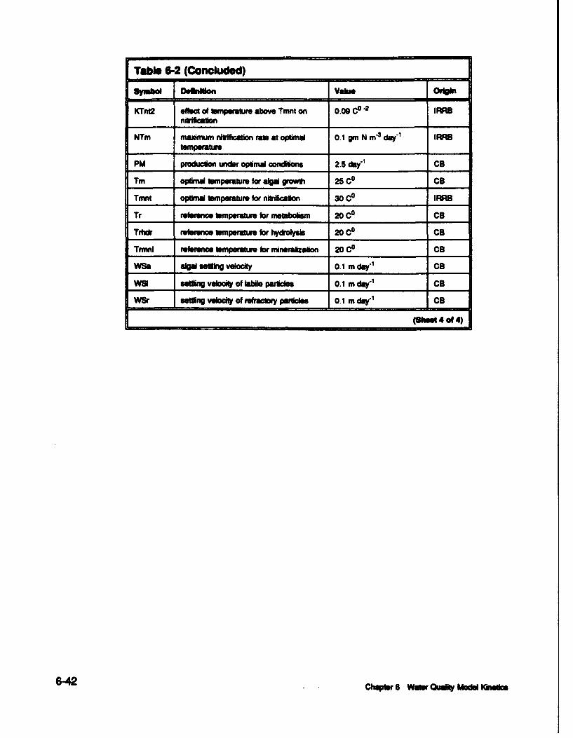
[ T a le 161-2 (C oncluded)_

_ _ _ _ _ _

KTnt2 effecit ot ampeaijre above Trmt an 0.09 CC - MRASmaificaion q

NTm maximum rMlflcafi ratis at optima 0.1 gmn N m-3 day-' IRRtB___ tampweramx __ _ _ _

PM production under optimal conditn 2.5 day-' CS

TM opimaleSmperamue for alga grofti 25 C0 es

Trmt opima Ismperature for niticaon 30 C0 MRSB

Tr reference lemnperature, for metabolism 20 C0 CB

Trhdr reference tamiperature for hydrolysas 20 C0 CDS

TinMI Weero enetmpersatue for mineralzation 20 C0 CDS

W8. alga se~in veloity 0.1 m duy' es

WOI seufn veloit Of laile partices 0.1 m d&f CS

WSr seOng velocit of retracery pawnie 0. 1 m dmy' CS

(Shee4eofJ4)

6-42 .Chaper 6 Wwatr Qua*t Model Kinetcs

Chapter VII: Linking theHydrodynamic and WaterQuality Models

Introduction

The hydrodynamic and water quality models are indirectly linked. Celldimensions, flows, and other information from the hydrodynamic model arewritten to disk for subsequent use by the water quality model The indirectlinkage makes efficient use of computer resources. An unlimited number ofwater quality model rums can be made using information put out by a singlerun of the hydrodynamic model. In order to link the models, output from thehydrodynamic model must be "mapped" to the water quality model That is,information in the x-y plane employed by CH3D must be converted intodimension-free information for use in the control volumes of CE-QUAL-ICM.

The simplest mapping is one-to-one in space and time. In one-to-one map-ping, water quality model control volumes correspond in number and size tohydrodynamic grid cells. Flows and other information are stored after eachtime step of the hydrodynamic model and the two models employ the sametime step. One-to-one mapping is the least efficient linkage procedure. Vastamounts of disk space are required to store all hydrodynamic information. Thewater quality model devotes an unnecessary proportion of execution time toreading hydrodynamic information and integrating the conservation of massequation using the hydrodynamic time step. For lengthy executions of thehydrodynamic and water quality models, the storage volume and executiontime demanded by one-to-one mapping are prohibitive.

Averaging hydrodynamic output before disk storage is one techniqueemployed to increase linkage efficiency. A second technique is the grid over-lay in which multiple hydrodynamic model cells are combined into singlewater quality model control volumes. Both averaging and overlays wereemployed in the linkage applied to Indian River-Relhboth Bay. Hydrodyna-mic information, computed at thirty-second intervals, was averaged into hourlyintervals before disk storage. The 2063 CH3D cells were overlaid into aCE-QUAL-ICM grid that contained 281 control volumes (Figure 7-1).

cOumr 7 LUntn to HYh. OW WSW Q•W fty MOdX 7-1

Figure 7-1. Water Quality Model Grid

Water Quality Model lime Step

The interval at which hydrodynamic output is writen is not necessarily theappropriate time step for use in the water quality model. Rathe, the waterquality model time step is determined by the stability requirements of thenumerical scheme employed to integrate the conservation of mass equation(Equation 6-1). Typically, the time step determined by stability limits isshorter than the output interval. An "autostepping" algorithm within the waterquality model determines the time step. The algorithm computes permissibletime step based on flow, dispersion, and cell dimension. If the time step isshorter than the hydrodynamic output interval, flow and dispersion are heldconstant until hydrodynamic information is updated at the next read operation.

7-2 ~~Chqbr 7 Linking Ow Hydrodnmic w4d Wassr OuadW Madmi

Inspection of the stability region of the one-dimensional QUICKEST algo-rithm (Leonard 1979) indicates sufficient conditions are:

At < A'X (7-1)-- U

and

At < A2 (7-2)

2D

At = time step MT)

Ax = cell length (L)

u = velocity (L T-1)

D = diffusion coefficient (L2 T-1)

The autostepping algorithm examines velocity, diffusion, and cell length ateach flow face of the water quality model control volumes. (These correspondto Qj I Aj, Dj, and 8xj in Equation 6-1). The time step is determined as:

At & 2 ~ (7-3)At = minimum a -, a. 2

ý u 2D)

a = constant that insures time step is less than maximum allowed (-0.95)

The flow face with the most restrictive time step determines the time stepfor the entire system.

Although the criteria expressed in Equations 7-1 and 7-2 are not strictlycorrect for application of QUICKEST in multiple dimensions, we have thus farfound the one-dimensional criteria sufficient to determine the time step inmulti-dimensional applications. The mean time step determined for the waterquality model was -300 seconds, an order of magnitude greater than thehydrodynamic model time step.

Chqpter 7 Linkng fhe Hydrodynamic and Water Quality Models 7-3

Linkage Testing

Linkage between the two models is accomplished through computer codewhich is not detailed here. Once the linkage software is complete, the linkagemust be tested to insure that transport in the water quality model compares totransport in the hydrodynamic model. For one-to-one linkage the testing isprimarily a test of computer code. When hydrodynamic information iscorrectly mapped into the water quality model, transport in the two modelsshould be identical. When temporal averaging and overlays are employed,factors in addition to coding require consideration. As the averaging intervaland overlay size increase, transport in the water quality model chi ,rges fromthe hydrodynamic model. Judgement is required to determine the acceptabletemporal interval and spatial resolution.

The ultimate linkage test is comparison of conservative substance transportin the hydrodynamic and water quality models. To perform our test, we setinitial salinity in the hydrodynamic model to zero. The salinity at the interfacewith the ocean was fixed at 50 ppt. The hydrodynamic model was run fort'Vty days during which salt was advected and dispersed from the ocean inter-fac :',v. the interior of Indian River and Rehoboth Bay. We ran the waterciua:i, - vdel using flow and dispersion from the hydrodynamic model andidentnicu initial and boundary conditions for salinity. One-hour averaging ofhydrodynamic information and the overlay grid were employed. Time seriesof salinity predicted by the two models were compared at several locations onthe water quality model grid (Figure 7-2). Each comparison (Figures 7-3 to7-7) comprised four plots. Time series of salinity predictions, output eachhour, were plotted in the upper left. Hourly salinity predictions from the twomodels were plotted against each other in the upper right. Salinity from bothmodels was averaged over two tidal cycles (=25 hours) and plotted as timeseries in the lower left. Tidal-average salinity predictions were plotted againsteach other in the lower right.

Perfect linkage is indicated when the salinity time series from the two mod-els exactly superimpose. On the corresponding scatterplots, all points will fallon the one-to-one diagonal line. The ideal is nearly realized at cells 52, 127,and 134. These cells lie in regions in which the horizontal gradient of salinityis small. At cells 247 and 117, which lie in regions of substantial horizontalsalinity gradient, agreement is less than ideal on the hourly time scale. Whenresults are averaged over two tidal cycles, however, agreement is muchimproved.

The linkage tests indicate the temporal averaging of hydrodynamic outputand the grid overlay are satisfactory for transport problems in which timescales equal or exceed two tidal cycles and spatial concentration gradients aremild. These conditions are typical in eutrophication studies. We conclude thelinkage between the two models is correct and suited for eutrophication model-ing in Indian River-Rehoboth Bay.

7-4 Chapter. 7 Linking the Hydrodynamic and Water Ouaity Models

127

117 12

Figure 7-2. Cells Selected for Transport Comparisons

ChplW 7 LUnldng the Hydrodynamic and Waar Quauity Mode 7-5

C., C.)

4.3

C.M CM )

C) =

0 0

c c

040N

c 0

00

C :0

0 0

o -n

C 0ý

LL

o- 0 hW7LfVt yWo n b uf M

C.., C.)

* ~00IWO. C.,

43 q

0

00

a cL~

0 0

CV,,

chqiem 7 LU*ing Ut. Hyeý@dy w Wi n WaK uAfty Modeb 7-

C-)

0 0

C3.

0 0

0 * 0

0 >.4

0z

0 0

cm C C

4.00

LD

7- *w w7 nqt i " wd o ~mCmt M f

-J-

0o 0

*V CD,

oo * 0

EMI I~ 2-4D

WO3 WON

I. 00N

.6. 09 C" 1 p0R L

isoi *SO 60. SO

ChmpW ~ ~~~~ 7 *qO y*wncadWWQf oe -

0 03

a9 9

-1

0

o 000

0 C0-CJ

c0

.J90,' ,SO ig. l * * c

7-10 Chpa 7 Lkft~q Ow !Vom m¶wd~ Vfj ~Guf km

Chapter VIII: Additional ModelInputs and Outputs

Introduction

Additional information, beyond loads and calibration parameter values, isrequired to operate the model. Additional inputs considered here are loadpartition, open-mouth boundary conditions, light extinction, and sediment-waterfluxes. Postprocessing of model state variables into more useful quantities isalso desirable. Derivation of BOD concentration and calculation of diurnalfluxes from model computations are detailed.

Partition of Loads

The quantities analyzed in the freeflowing streams and in the point-sourcedischarges required mapping into model state variables (Table 8-1).

Table 8-1

cmepodenme of Loads ad Mdel Stite Varibles

Obs rva tion m e" hio S aw VIluls

Dissolved Organic Carbon

Biochemical Oxygen > Labile Particulate Organic CarbonDemand

Refractory Particulate Organic Carbon

Dissolved Organic Nitrogen

Total Kjeldahl Nitrogen ý> Labile Particulate Organic Nitrogen

Refractory Particulate Organic Nitrogen

Dissolved Organic Phosphorus

Total Phosphorus Labile Particulate Organic Phosphorus

Refractory Particulate Organic Phosphorus

ChWWtr a Addiikm Model lnp and Outut 8-1

No exact conversion of BOD to organic carbon was possible but reasonableempirical correspondences were employed (Chapter 3). The derived totalorganic carbon still required partitioning into model state variables, however.Relationships used to derive loads of model state variables from observedloads were:

DOC =FDOC *TOC (8-1)

LPOC = FLPOC * (TOC - Doc) (8-2)

RPOC = (I - FJIoc) Troc - DOc) (8-3)

TOC = total organic carbon (gin m 3)

DOC = dissolved organic carbon (gin m-3)

LPOC = labile particulate organic carbon (gmn m-3)

RPOC = refractory particulate organic carbon (gn m-3)

FDOC = fraction of total organic carbon that is dissolved

FLPOC = fraction of particulate organic carbon that is labile

DON = FDON * (KN - NH 4) (8.4)

LPON = FLPON * (T•N - NH4 - DON) (8-5)

RPON = (1 - FLPON) * ( - NH4 - DON) (8-6)

TKN = total KjeldahlI nitrogen (gin m-3)

NH4 = ammonium (gin m-3)

DON = dissolved organic nitrogen (gn M-3)

LPON = labile particulate organic nitrogen (gin m-3)

8-2 CWb 8 Mi•iOnd ods kqxa wW Ouqinu

RPON - reftory picultMe or ic nitroM (g9i &1 )

FDON = fraction of total organic nitrogen that is dissolved

FRON = fraction of particulate organic nitrogen that is labile

DOP - FDOP * (TOTP - PNO) (8-7)

LPOP - FLPOP * (TOMP - P0 4 - DOP) (8-8)

RPOP -( - H-POP) * (rOrP - P0 4 - DOP) (8-9)

TOTP = total phosphorus (gm in)

P0 4 = dissolved phosphate (gin izn)

DOP = dissolved organic phosphorus (gin m-3)

LPOP = labile particulate organic phosphorus (gin m-3)

RPOP = refractory particulate organic phosphorus (gin m"i)

FDOP = fraction of total organic phosphorus that is dissolved

FLPOP = fraction of particulate organic phosphorus that is labile

Initial values of splits were adopted from values employed in ChesapeakeBay tributaries. These values were refined during calibration of the IndianRiver-Rehoboth Bay model (Fable 8-2).

Open-Mouth Boundary Conditions

Cnnaons at the junction of Indian River Inlet with the Atlantic Oceanwere specified primarily using data collected offshore of the inlet by the EPA(Chapter 2). Observations were available for 12 of the 36 months covered bymodel calihration. Boundary conditions in months for which no observationswere available were filled in with values observed in the same month in alter-nate years or values observed at the mouth of Chesapeake Bay. Good corre-spondence was observed in temperature, salinity, chlorophyll, phosphate, anddissolved oxygen between observations collected offshore of Indian River andat the bottom of the Bay mouth (Figures 8-1 to 8-5). Salinity boundary

OChWp S Addind Mox Inpft and out 8-3

Table 8-2

Dissolved and Labile Fractions of Loads

I Nopookd-,oume VOA Pah Vaius

FDOC 0.8 0.8

FLPOC 0.0 0.15

FDON 0.6 0.8

FLPON 0.0 0.1

FDOP 0.1 OA

FLPOP 0.0 0.0

conditions for July and August 1989 were specified to match observationscollected within Indian River Bay during those unusually wet months.

Light Extinction

Light extinction was specified based on disk visibility measures collectedby the Academy of Natural Sciences and the College of Marine Studies (Chap-ter 2). Disk visibility was converted to light extinction via the relationship:

KE-= 1.45 (8-10)DV

KE = light extinction (m-1)

DV = secchi depth (m)

Light extinction in Indian River-Rehoboth Bay is strongly affected by chlo-rophyll concentration (Figure 8-6). Light extinction input to the model isbackground extinction independent of chlorophyll. The effect of chlorophyll isadded to the background value based on computed chlorophyll concentration(Equation 6-9). Consequently, the effect of ambient chlorophyll had to beremoved from the observed light extinction. Light extinction in the studysystem may also vary seasonally or regionally. In order to quantify the influ-ence of chlorophyll and detect seasonal and regional trends, a model wasproposed:

8-4 Chaptr 8 AddiMnal Mode Inputs and Outpt

25

-'--ae ----

20 W 4 681RivOeUr12 0/ a0

~10 /,A

5

MONTH

Figure 8-1. Temperature at Mouth of Indian River and Chesapeake Bay

35 -

0 1

30 0

0 Wnian River

20 + I I

1 2 3 4 5 6 7 a 9 10 11 12

MONTH

Figure 8-2. Salinity at Mouth of Indian River and Chesapeake Bay

Chpbr 8 AMid•" ModaM I" and OutpM 8-5

30 0

A Chmapeke

ee o Indian River

04-10 2 3 4 5 6 ? 8 9 1 1 1

50

*20

0.1 5

0.045 --- Chesapeakeo

0.04 o India RLiver

0.035 0

0.035

0.15 2 S 9 1 1 1

MONTH

Figure 8-4. Phosophate at Mouth of Indian River and Chesapeake Bay

0.08 .5- 8I

i o a0.045 // "apak

g\

0.012 a / 0

0.005 o' /

0 i I I I I I oo,

1 2 3 4 5 6 7 8 9 10 11 12

MONTH

Figure 8-4. Phosphate at Mouth of Indian River and Chesapeake Bay

8-6 Chqpsr S Adclni~m M•odal 0nput and Outputs

12

10

Fiue -, islvdOxgnatMut f nin ieradChesapeakeBy8

2o RniRiver

0 I0I 0000

I A 3 4 5 6 7 a 9 10 11 12j MONTH

Figure 8-5. Dissolved Oxygen at Mouth of Indian River and Chesapeake Bay

0 Region1, 3 07 a Region 2

0 4

6 00m g cmINI 0 o

0000 0o 03w CO OD Oo4DD O

.4-,I 0~ 0 O O 0 ~

C.)

00

0 - .. ... 'I , . . . ..... i . . . . . I. . . . . . .i

2 3 2 3 101 2 3 102 2 3 10-

Chlorophyll (mg/m**3)

Figure 8-6. Relation of Light Extinction to Chlorophyll Concentration

Chopr 8 Adjo Mod lnpus an 0u€ 8-7

KE = a + bRI + cR2 + dR3

+ s(ý79Jday~+ f cos2. X Jday + .gCHL (-1365 365 (

a = annual mean background light extinction (m-1)

b = incremental light extinction in Region I (m-1)

c = incremental light extinction in Region 2 (mn1)

d = incremental light extinction in Region 3 (mn1)

RI = I in Region 1, 0 elsewhere

R2 = 1 in Region 2, 0 elsewhere

R3 = 1 in Region 3, 0 elsewhere

e, f = parameters that determine amplitude and phase of seasonal variation(m"1)

iday = julian day

g = effect of chlorophyll on light extinction (m2 mg"1 Chl'a')

Stepwise regression was employed to evaluate parameter values. Observedextinction was treated as the dependent variate while region, julian day, andchlorophyll were treated as independent variates. Three regions were defined(Figure 8-7): Region 1 - Lower Indian River, Region 2 - Upper Indian River,Region 3 - Rehoboth Bay.

The analysis (Table 8-3) indicated that chlorophyll was the primary deter-minant of light extinction in Indian River-Rehoboth Bay. A seasonal trend,independent of chlorophyll was also detected. Background extinction in UpperIndian River was greater than elsewhere but that no difference existed betweenLower Indian River and Rehoboth Bay. Monthly values of background lightextinction, that accounted for seasonal and regional variation (Figure 8-8),were input to the model.


Sediment-water fluxes of oxygen and nutrients can be a significant influ-ence on water quality in shallow systems such as Indian River-Rehoboth Bay.One component of the sediment-water system in the shallow bays is a layer of

8-8 Chat, B Adeilnal Model InpuB w W f utp

Figure 8-7. Regions in Light Extinction Analysis

Table 8-3Analysis of Ught Extinction

Itur Valu. CuMtWS 2P

a 1.40

g 0.016 0.30

0 -0.56 0.35

f -0.74 0.40

C 0.88 0A7

benthic algae that occupies the sediment-water interface in regions where lightintercepts the bottom. Actions of the benthic algae modify the sediment-waterfluxes that usually occur in a darkened water column. Photosynthesis by ben-thic algae may induce an apparent sediment release of dissolved oxygeninstead sediment oxygen demand. Nutrient uptake by the algae may induceapparent sediment nutrient uptake when release to the water column isexpected.

C s AdMwW Mom I" an O- f 8-9

8 0 Observed, Region 1. 3a Observed, Region 2

7 Time Series, Region 1, 3 o7 - Time Series, Region 2

6 ao 1 o

0.5 o o o013 a a

040.bJ0 MO a i a 0U

2 0 0 O[ 0 0 0 0-U0 00

000 30 60 90 120 150 180 210 240 270 300 330 360

Julian Days

Figure 8-8. Seasonal and Regional Variation in Light Extinclion

A series of empirical models of sediment-water fluxes were constructedbased on observations collected in Indian River-Rehoboth Bay (Chapter 2).Raw data supplied by the principal investigator consisted of replicate measurescollected at varying light intensities. The replicate measures were averagedand scientific units were converted to units employed in the model. Simulta-neous measures collected in light and dark were combined into daily-averagefluxes that occur during day-night illumination cycles. The observations,treated for analysis, are reported in Table 8-4.

Empirical models were formulated based on examination of the data, onexpected actions of benthic algae, and on typical sediment-water interactions ina darkened water column. The sediment oxygen demand model was:

SOD = SODbe (T - 20) + bLight (8-12)

SOD = sediment oxygen demand (gin m"2 day-)

SODb = sediment oxygen demand at 20 Co in a darkened water column

8-10 Chopr 8 AdionW Mol I"pw wd &W uwm

Table 8-4Observed Sediment Water Fluxes

Station Tamp, Light, SOD, NH4, NOr P04,c ISMgley gm mr mgg m-2 mg mi mg9 m

1 12 157.5 0 0

12 0 -0.784 52 0.45

2 12 157.5 0.505 -5.7 -0.76

12 0 -1.25 34 0

3 12 157.5 0.233 -5.5 -0.22

4 12 6.75 -0.894 39.5 -16

1 25 63 -1.12 27 1.44

2 25 15.3 -1.06 34 8.56

25 0 -1.54 150 10.4

3 25 90 -0.209 5.9 0

25 0 -1.15 107 6.45

4 25 0 -3.48 147 9.67

a = constant that expresses influence of temperature on sediment-water

fluxes (C0 -1)

T = temperature (C°)

b = constant that expresses influence of light on sediment-water fluxes(gm m"2 langley 1)

Light = illumination at sediment-water interface (langley day"1)

By convention in the model, fluxes from sediment to water are positive.Fluxes from water to sediment are negative. The empirical model indicatesSOD is negative (oxygen flows from water to sediment) when no light is avail-able at the sediment-water interface (Figure 8-9). The magnitude of SODincreases as a function of temperature. The availability of light at the bottommakes SOD less negative. At low temperatures and high light intensity, thebottom gives off oxygen. At extremely high temperature, however, SOD isnegative despite light availability. (To aid in interpretation of the functions,Table 8-5 presents a few reference values of temperature and light.)

Chpter 8 AdftonW ModM Irpts and Outu 8-11

1-1

10W

-1.

-.5

Figure 8-9. Effect of Temperature arid Light on Sediment oxygen Demand

Table H-TeRMpature Nd Light at SedinentWater Metefe at Mmmii Deph of MndanRlvs-Rhhoboth May______ ________

mumi TmnyRatum, U^t Rgion !~, 3. U0It% Rqlon 2,S CP EWE! dmy I.'., m

January 5.3 205 46

July j 26.6 Is 4

The ammonium flux model was:

NHAX= N 4 f'b cCF - 20) - b PN Nlim Light (8-13)

NH4flx = ammonium flux (gmn m-2 day-1)

NH4flx = ammonium flux at 20 C0 in a darkened water column

8-12 Chw 8 AdManw Mudm lnpefs aw Ouspu

PN = algal preference for ammonium

Nlim = nitrogenous nutrient limitation for algae

Definitions of remaining terms are the same as for SOD (Equation 8-12).

Ammonium flux is positive, from sediment to water, when no light is avail-able at the bottom (Figure 8-10). Sediment ammonium release increases as anexponential function of temperature. When light is available at the bottom,ammonium release is diminished. Under strong illumination at low tempera-ture, sediments take up ammonium. The nutrient preference and limitationterms are identical to the terms specified for phytoplankton (Equations 6-4 and6-21). These terms prevent sediment ammonium uptake when none is avail-able in the water column.

120100 -

T....

4so...... T=20

40

2-6O~-so ISO10

-40 -.

-60-

PN * Light (laneyu/day)

Figure 8-10. Effect of Temperature and Light on Sediment-Water Ammonium Flux

Nitrate moves in both directions across the sediment-water interface. Thiseffect is influenced by concentration in the water, independent of benthicalgae. When nitrate is abundant in the water, nitrate flows to the sedimentswhere it is denitrified to a gaseous form. When nitrate is absent from thewater, small sediment release occurs due to production by nitrification in thesediments (Figure 8- 11). The empirical nitrate model was:

CWe 8 AdMind Mode Inp&t and Out"M 8-13

20

S-20 2 0.4 0.6 0.1 1

-40

~-60 - - -- T-10

0T-20

0 ..... T30-I00 .... =0"'

-120

N03 (ginm*3)

Figure 8-11. Effect of Temperature and Concentration on Sediment-Water Nitrate Flux

NO3flx -s (NO3sed - NO3wat) e a CT- 20) 14)

-(I - PN)Nlimbb ght

NO3flx = nitrate flux (gin M2 day-)

s = sediment-water mass transfer coefficient (m day"')

NO3sed = sedimem rniae concentration at sediment-water interface(gin m-)

NO3wat = water-column nitrate concentration at sediment-water interface(gimn M)

Definitions of remaining terms are the same as for SOD (Equation 8-12) andammonim (Equation 8-13).

No influence of benthic algae on nitrate flux could be discerned in thelimited data base. Potential influence of benthic algae was included in theempirical model, however. The influence of benthic algae on nitrate is

8-14 Ch• s 8 Adjia Mdmi Iwu u Oumpu•

identical to the influence on ammonium except that ammonium in the watermust be first exhaued before nitrate is consumed. The effect of benthic algaeis to increase removal of nitrate ftom the water column beyond the amountconsumed in deniurification (Figure 8-12). The enhanced removal occurs onlywhen light is available, however, and increases in proportion to lightavailability.

soT,-20C

-S ..- ' - -- o'z- -. 0.4 0.6 0.o I.0

-20

-2 ............................... * ... ....

N03 (Xmft*"3)

Figure 8-12. Effect of Concentration and Light on Sediment-Water Nitrate Flux

The phosphate flux model was identical in form to the ammonium fluxmodel:

PO4flx = P4flxbea(T - 20) - bPlim Light (8-15)

PO4flx = phosphate flux (gin m-2 day"1)

PO4flxb = phosphate flux at 20 C& in a darkened water column

Plim = phosphorous nutrient limitation for algae

Definitions of remaining terms are the same as for SOD (Equation 8-12) andammonium (Equation 8-13).

Chatr 8 Adi*onmd MDo" inputs &W Oututs 8-15

Phosphorus flux is positive, from sedim... ,o water, when no light is avail-able at the bottom (Figure 8-13). Sediment ,piosphate release increases as anexponential function of temperature. When light is available at the bottom,phosphate release is diminished. Under strong illumination at low temperature,sediments take up phosphate. The nutrient limitation term is identical to theterm specified for phytoplankton (Equations 6-4). This term prevents sedimentphosphate uptake when none is available in the water column.

15 T=I0

T=20

... .. .. ......... T=30

50 -- 1.150200.5.

-10s

-155A.: -105 "

-20

Plim * Light (langleys/day)

Figure 8-13. Effect of Temperature and Light on Sediment-Water Phosphate Fklx

Parameters in the empirical models were initially evaluated through nonlin-ear regression. Initial values were refined for uniformity and to optimizemodel calibration. Final values are presented in Table 8-6. Sediment-waterfluxes determined by the functions are compared to observations inFigure 8-14.

Computation of BOD

The biochemical oxygen demand (BOD) analysis combines measures of theconcentration of oxygen-demanding material and the oxidation rate. BOD isnot a model state variable but the BOD of quantities computed by the model

8-16 C hatr 8 Addional Model Inpum and Output

Table 8-Parameters In Empirical Flux Models

gm FIbx, ,. $IClgmm day-' gm m1 _wow, mjfl nNm

Sediment -1.45 0.05 0.011OxygenDemand

Ammonium 0.07 0.05 4.5x10-4

Nitrate 0.05 4.5x10-4 0.1 0.03

Phosphate 0.009 0.05 l.lxl0"

SOD 0 150 NH4 S

0 gm/m**2/doy 0 125 rmg/m**2/day

0 0

250

100

Model Model

NO03 , P04 000

8

> >6

L.. t-D o 4)cn cn-10- -_a5

C) 0

2

0 0

-150 0

-20 -2 .-20 -15 -10 -5 0 5 -2 0 2 4 6 8 10 12

Model Model

Figure 8-14. Observed and Modeled Sediment-Water Fluxes

Chats Addtoe Mode npt anda Outu 8-17

can be calculated for comparison to five-day BOD observations. Model BOD5

was computed:

BOD5 - AOCR B (I - e - 5BM) + AOCR DOC (I - e - 5 Kdoc) (8-16)-5 NTm

+ AONT NH4 (1-e (1 -)

BOD5 = five-day biochemical oxygen demand (gin m"3)

AOCR = dissolved oxygen-to-carbon ratio in respiration(2.67 gin 02 gin C-1)

B = algal biomass (gin C m-3)

BM = basal metabolism (day-1)

DOC = dissolved organic carbon (gin m-3)

Kdoc = respiration rate of dissolved organic carbon (day-1 )

AONT = mass dissolved oxygen consumed per mass ammonium nitrogennitrified (4.33 gin 02 gm 1 N)

NTm = maximum nitrification rate (gin N m-3 day-1)

KHnnt = half-saturation concentration of NH4 required for nitrification(gmNm-&)

The relationship is an adaptation of the formulae for oxygen consumptionexpressed in Chapter 6. In the computation of BOD, oxygen is considered tobe available in excess and ammonium is considered to be much less than thehalf-saturation concentration, KHnnt. Since the BOD analysis is conducted indarkness, algal respiration is considered but not photosynthesis.

Diurnal Dissolved Oxygen Fluctuations

Algal physiological functions that create diurnal dissolved oxygen fluctua-tions are not well-represented by the conventional photosynthesis and respira-tion relations employed in eutrophication modeling. Additional influences ondiurnal fluctuations, particularly macrophytes, are not represented at all in themodel. Consequently, the preferred means of computing daily-minimum dis-solved oxygen is through a relationship to predicted daily-mean dissolvedoxygen. The relationship was developed by fitting a sinusoidal function (Fig-ure 8-15) to each diurnal dissolved oxygen measure:

8-18 e 8 :dfan M npum wo& Ou"s

I0 o0

7 Dar 7

4 4

0 , 1

Ho=% M•iA 25-2. ,M

Figure 8-15. Sinusoidal Fit to Diurnal Dissolved Oxygen Data

DO -a + bsix{-ZTJ)+cco{ TJ (T-17)

DO = observed dissolved oxygen concentration (gmi 0 2 m3)

a = mean dissolved oxygen concentration (gm 02 m-3)

b, c = parameters that determine amplitude and phase of diurnal DOfluctuation (gm 02 M)

Parameters a, b, and c were deternined by regression. Amplitude wascomputed:

A b2 + c2(8-18)

A = amplitude of diurnal DO fluctuation (gim 02 m-3)

Ob em 8 IdUWd AM Ifnpts and ut 8-19

Next. regression was used to relate amplitude to chlorophyll concentration.The resulting relationship was:

A = 1.51 + 0.033 Chl (8-19)

Chl = chlorophyll 'a' concentration (mg m-3)

R2 for the regression was 0.76. Worth noting is that a diurnal fluctuation of1.5 guim 02 m-3 exists in the absence of algae (Figure 8-16) and is presumablycaused by aquatic vegetation.

To compute daily-minimum DO, dalfy-average predicted chlorophyll issubstituted in Equation 8-19 to obtain amplitude. Amplitude is subtractedfrom daily-average predicted dissolved oxygen to yield daily minimum.

5

4.5

4

" 3.5

A2.5

2

S1.5 bea

1 -

0.5

0 20 40 60 t0 100

Chlorophyll (rn/m**3)

Figure 8-16. Effect of Chlorophyll on Ampitude of Diurnal Dissolved Oxygen

Flictuation

8-20 ChW6r 8 AMiand Mda Is ENO Oupu

Chapter IX: Water QualityModel Application andAnalysis

Water Quality Time Series

The primary means of calibrating the water quality model was throughcomparison of modeled and observed time series of water quality constituents.Time series were compared in eight model cells (Figure 9-1) selected to pro-vide spatial coverage and a sufficient number of observations. Calibration wasan iterative process in which kinetics coefficients (Table 6-2), sediment modelparameters (Table 8-6), and load fractions (Table 8-2) were adjusted toimprove model-data agreement. Calibration ceased when no additionalimprovement was possible. The final calibration time series are shown asFigures 9-2 through 9-9. Observations are grab samples collected within amodel cell. Symbols indicate the source of the observations. Model resultsare daily average values for the cell. The temporal origin (Year 0) is Janu-ary 1, 1988. Time series cease (Year 3) on December 31, 1990.

Longitudinal Transect

Additional insight into the calibration status was gained through comparisonof observations and model results along a longitudinal transect that extendedfrom the Millsboro spillway to the mouth of the Indian River inlet. Transectswere plotted for the summer of each calibration year (Figures 9-10 through9-12). The spatial origin (Km. 0) was at the spillway. Data collection alongthe transect was not synoptic. Neither were observations collected at uniformintervals throughout the summer. Consequently, no attempt was made to pro-duce a summer-average from the data. Grab samples collected in the monthsof June, July, or August were plotted at the location of the observation. Thesewere compared to summer-average model results. Point-by-point agreementbetween the model average and grab samples was not expected. Rather, theplots were used to assess observed and predicted spatial trends and approxi-mate agreement in concentration.

Ch*Ww 9 Ww. Ouuy Mod Appbcawn and Amdym 9-1

Figure 9-1. Grid Cells Selected for Time Series Presentation


Time series of modeled sediment-water fluxes (Figures 9-13 through 9-20)were produced at the same locations as the calibration time series (Figure 9-1).By convention, fluxes from water to sediments were shown as negative values.Positive valuers indicated sediment release to the water column. The "Carbon -

Oxygen Flux" time series included carbon deposition to the sediments andsediment oxygen demand. The "Nitrogen Flux" time series included particu-late nitrogen deposition to the sediments, sediment-water ammonium flux, andsediment-water nitrate flux. The "Phosphorus Flux" time series indicatedparticulate phosphorus deposition to the sediments and sediment-water phos-phate flux.

Interpretive Information

Time series of interpretive information available from the model (Figures 9-21 through 9-28) were produced at the same locations as the calibration timeseries (Figure 9-1). One time series indicated the computed nutrient and lightlimitations on algal growth (Equations 6-4. 6-6). Potential limitation rangedfrom zero (complete limitation on growth) to unity (no limit on growth). A

9-2 Chaptr 9 Water aualt Mode A• iaon wd Anaysi

00L IS

0 0-C-

L -~ 0

o1 >0-0

(3 __ _ _ _ _ _ Ec

M ) +

0 0

ELI +i i

0

z L

m +

z+

Ctqr9Wawe Quality Model abnndAmyi9-

++

C~+

+

+ +J

+0 +

+++ +I

* +

00

wr

m o +

0:

LI LLI

LJ

+

+z +

zr 0

--1 CC 0 0

CHNW/Ws E£wW/Ws O

cN

9-4~~~~ Chpe 9 Wateuality Model Apocatimari uAmaya

N

+ ++ +

0 + +

+

0)C3

0-)

+0- ++.-) 0.

CD 0)0

0~0

-+~ 0F- F-

+

30 f0o -))

0 04--iL 0

4.)z +>

N +00

r-, (Ao

Emxw/w U

EWNW C4

LL

-hpe 9 ae*0lyMMAphao n nls -

+

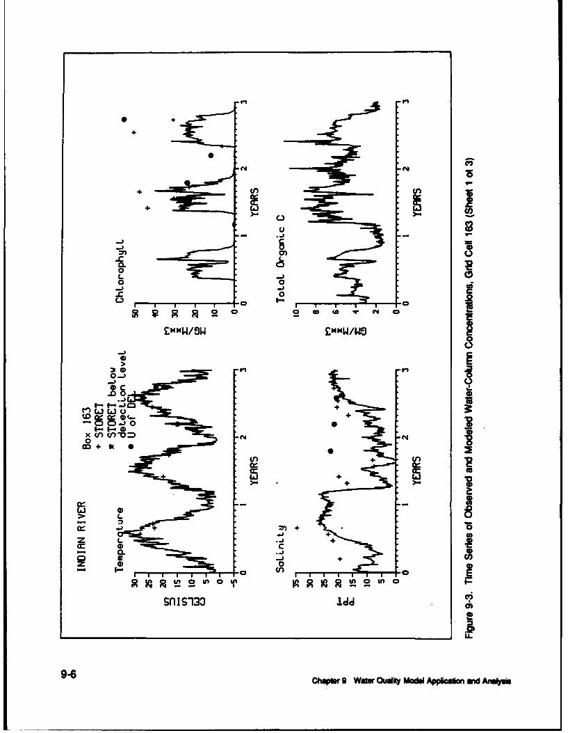
00L C9

0

C-)

0-)

00 c

.0 0~C

0 r

o -,-

z a La +

0 .

zf 0

Li 4.

9- Chpe 9 ae ult AmrmAp 1a - nhi

t+

z

++

0 -j

L -

+ -*j +

cm - 0C

I- F- C3InJ 0L IOUI Ca i a i

1- 1- - 0N -

o +)

M cca

zI + (

z c- LAC To -T--C

00CD to~ 4w C4 0-

LL

Chopwg 9 Water Quality Model Application and Analysis -

+

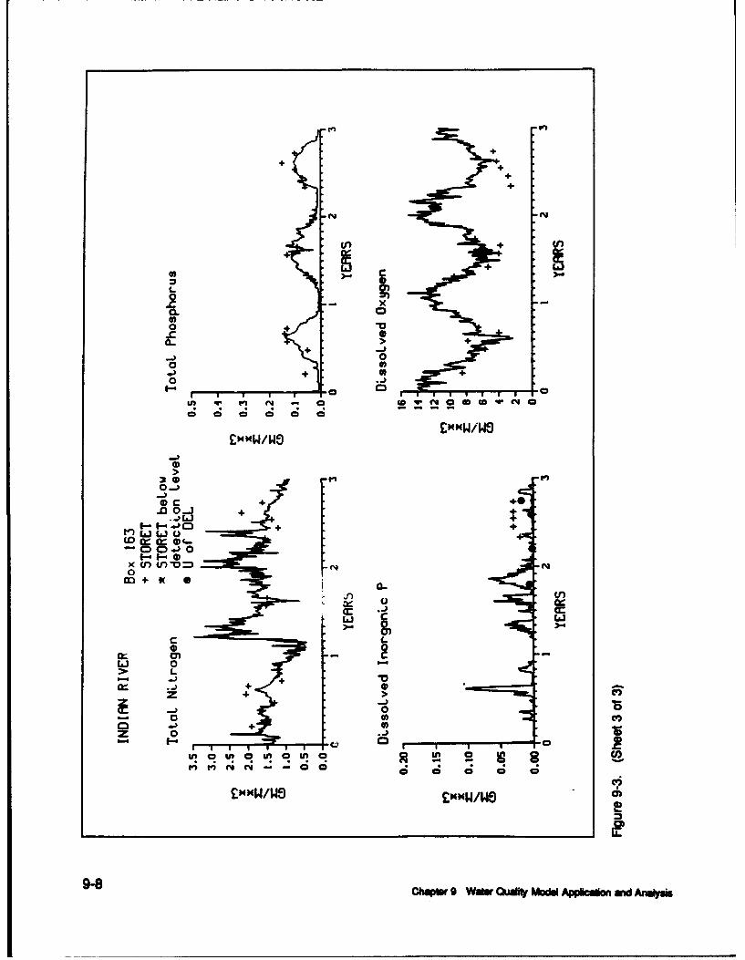
00

0-)

0 c+ +0

+ +

0 ,

o +3

Sf q p N - C a=@iA N

Li 0Ln

+ V)) + >

M c +

z 0S

r) Cm) 0I-; C;-.0C

EWN/s Nmww)00L

~~LS

9-8 hWW9 WA Quft oM Apkaon ad Am-i

00

LAL

0 -

0.C-)J

o9 0.s.2

£r 0

0 .

++

.CC cia

0:

L ++-I

0)0

ct~tr 9 ater~j~yModLApiuonmdnuys

L

CC

)0 Z

4.) W IL

9 5') 0

0

4.) 0

Z a MIn 0 n ~ 0 a In 0 IflW

o +)Scc

cc 0- +Y... ) Li

7- -. OCD LiiLii -1

U Lii

Cf

9-0CL 9WWify o pkimm n"

+.

L CD

+. CD . r

0 V

CL >~o0) j

0

-0

o 0)

C. 4 -) 0

0

++

CC)

CD c L4) 0

00

z mrc 0

z 00

ChmWhu 9 Wawa OQalty Moal pplcain &Wd Analyis

+

UU

0-)

-c+

C3)

o -r) Oa

+ (x ++ + ur)(r c rrau

I-. I- )

+ +4 +

4. c

U.

9-12 hOPW9 Wa Qu~d Mo"Apocm WWAmm

* +

4 >W

z +

+

L 0 - -0

zI%/W Eww/ +

*) c. -)L.L) 00

00co + 0o q n a i

-~cr 0 0 0N -

Sc-

z +

00R+ R( RS ?R 9ý l .1 C

WA +n *(eAY- 00 2v

ENNW/E) EHWLi

Chaplrg Wlwifyid pk mad*"93

+ + (n

I= +cc +.

c >4

LI

00

0. +

C2 >-j

0

Q 0 CD 0 0 CD

EXNW/Ws

30

4)c +++ +

to LL. Lai 0+

003 +

CYcc L-

4) 00b

LM

z +

0 I

0 0))Z 0S

V, I

9 &ý V! C

9-4Chqmsr 9 Wasr CQuWit Mode Appliaion wW Anulpft

N eCa

C)C.00

0 00

C, -0 *0P

£XHW/sw H/sr

5W ++

.00..) +.0 0 -J +.

r3 + r. ca

0

CC +

+ + w+ (-p

oJ t

C--

L to

0.0

U.

ChWIW 9 WatW Oudity Mode Applicmalin d Analysis 9-15

0 +

w + ++

+ + + n

N +

++

A) +

+

0 -0

L -r 1 -. rC

-,ý r*09 U! 9 U

0 0 D 0 Q C

L) 0

UE U

00

rn 0

-~cr 0 0 0N -

Oc +(0 0O 0

.-) Q J E1*-- Q.'

C? C?. LI CV)

to4 r) C4c0 ; c

UU

Chpe 9Wtr ult Modl Apiai AAsi

+ 7.

+ V)+

+ CK +

+ a+ M+ Li + LI

L 0

xCL (D0)00)

-C 0

0o 0)

0 0 0 0D Q

£~w~w/WS

3.0 ++

0) 4.+ ++00- +

+ +4+

C3 +to Li L +

(J C0 C.)- 0F-. (-. 0)

07

+ LA(n

cc+ L c u L

0Ic La) 0

F- 0.

C) M)

0A +0

0 0~ ,0 I I I .IC

£!M !R n /iW8Cf

Chapter 9 Water aluality Modlel Application and Analysis 9-17

+ cN

+0 f

ELI >

Q C)

-c C N

L L0'

0

z"Mw/ow ENW/Wo

00

++

DI) 9 3

, )E

C aE ) C3 0

w Sr 0.C) C) -) 0l

I- -. -a)

0..

co + +cn + (-

9-1 mhps + ~rOdt oe ~c~nmdAayi

* +

E+++

CC+

LI

-C;

.4) *0

zr *r 0)

0 .00)

00

+ E,++

0 0 +..C. -) LIN

I LI I I I

c"H/J Emow o ý-

I-. I-~d0

ChpeX ae Qulty Model Npiato aN rlm91

+ +iLL

L+

0 x

(A -0

00

(L> oIa. 0

0 0)

00

0 0D 0 C

o -)++

a) c +.0 0-1 + +

+

0o oI 0a3C.

x- (f) (no N0

CD + 0 a..+ u.

LIJ c Li0)

c La, 0

0-L -0

C) 0.

Li 0

9 4.,C

o in cm 0 HN2 Wo

U.

9-20 Chapta 9 Wate Oudity Iode Appkca~o wW Anulahm

+

+ Cf

00

L 0

0,C,'+0

-- -T - I I

0

00

C., 00 0

0~

aJ IAJ

m- LI

0 L LC

0Eli 0( I T I I

LL

ChW+ 8 o ufyMrsApkk WAa92

* +

00

0L M C - -~ -

0-)J

0 C) 00

G r)c) m4

(n +

Liu

-, +co _ _ _ _ _ *

oý or 0 .~ fl C ) C U

o -o

CD (+

9-22 ~ . oh W9WWOud m picmw r*

cr. +

0 Z)

0- >

00

0)

+ -J+

'00o00

cc ' +oC6-(f (f) -

o ) -

oc + >

C). -j i .

00

00

0)ro Lo0t 0t

0 C;02~w CO

ChaP -oae wlyMmApk~ i nl"92

0~

0 0

-c~ CD

a. 00 -0

.D 0

C) 2

M 0 ... + +.ac +-.~ oz

LL) +a. Ci.)

0 L

Q 4.E4

.U, +D t

o LD

9-2 C hp 9 I uyMMAomma mv

+ +cr +

++

+ -0 + (Id +

0 )0 Cz

z0 O 00 +

L6 0x r () =

00

Z -O

ooC)) ca N

EL) S1jci

X CD0C N N

I+ ILL

Chmpher~( 9 Wate Cl(t odlApianadAalss92

+

+

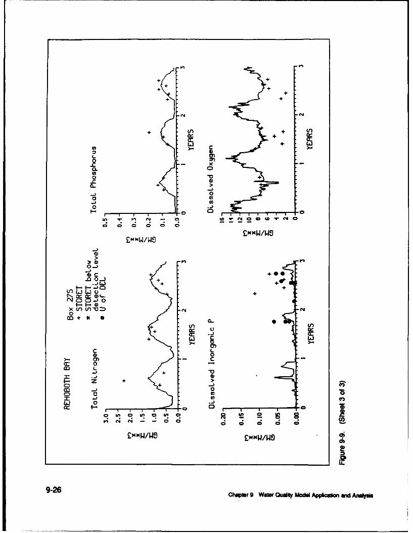
0 N

0 +

00-C.0- >

0j0.0

0)-0

1) 0 3

0 0

-0 0 j

I- 1- 0 _ _ _ __ _ _ +

C)0 0 0 0

0)

SC +)

U c LiL.3C

00

m0.0+ U

+ -j L0,

C CD

0) 0 ; C

omww -NwwOoL6

+ -.

9-2 Chate 90ae ult oMApcsmaWAw

coI0C

cc w0

u.

0-2

C.)o. L E0 eL ... LA

.C 0

a)

o -) N

-0 0O3.- 'L.P1

+ +-

01- 0

OD +

Li~i Uiw +o

U-) 4+

'a lCL-

ChmpWr9 WwalrOudiy Model AppiUSUansd Aradyels 9-27

+ +.

o +i

00+ ID

L- 0 +

z + +z Tr- 0

C.. N1 0 N l0 4 N - 0 C

00

-0 0 -j *

oo -)m

... LiJ

10

+ +

00n 0

0) + 0 *Li 0 L 0 L

0 0

C + 4+C;C;

ENW/i Emx 10

+ 44W

9-2 Chpe 6a kiyMM pbamai n

+ + Li ++L

I-- ÷ -

0 , 0

L-- 4-+ ,'-0,4

f~o

+ * -+ x + +0) + ++

c.. o I [

+- + .J+-, 0

.1Li.

+ + + *

.0 0CD__ _ __ _

Ifl co w w C4 0Q 0q 000 0 CD 0 0

o -)

.-) LI-0 0 -

0 ..jI.-.

04 CýO 0

f--- F0))w

0) ) + V)(f

w a-++ U

0j 0)

0) Ukl 0 n a i f

0 0 0 0 (D

-0)J + /WSz >-

Chqls + W+e u~~ oa ppiaisdAayi

0

U+ 1. 1

+ + e.

+ +

+ ~ LE0+ + e

L U.

0~ 0

I is

.2

U)

o -)

.-) c

U Li 0w of.-

0-I- 0

Li 0i

(n~ + 4+ +.- +

+ *1i

+~ ++ .. * .B0

Z L + +CaS CE 0 + + .j 4 N-

0)

Is

9-30Chapter 9 Watinr Ouafty Model Appicadon aim Anlaink

LiJý-, +

+ +

+4+ + +z

+ + w.)+ + + +

L N 0 M4'+ + 4.) + +

0z I I I I. r--T- -r -- I I -o0

9 inc 9n o! 9n U! 9 9n a e a eM~N - - 0D 0 M~ N N - - 0 0

-C0 0 -.0 ..)

.JJ L)0 0 0

004. 0f-4f-40 w

+41 +

++

C~

a3 ++

I I-

Cbqibr 9 Waty Oudky Modael Appkelon aid Anads~s 9-31

CD CD

4. 1W C

0) +

.C + x 4

0. w 0

+ + )0)

CD 00 )+

£'HW/Ws

cmSw

II.00 -j

C)] C). 0.

I- f-S .

-r CL a-+- I-

(n c + CO C0) 0

Ix) 0)w -L++

zz + -

CC 0- 0 to)

41 + + Uz 0

ENNW/Wa

9-32 Ctiqh~r 9 Waas Cluel Miodul Aplamoan end Andjyft

40 40

0 +

004

++ 0

r 1.0U9 V______ RR____________W V q D

a)," +4 -- -h

00

+a~J + - + +a)- (nl (.

0 ~ + + ~ Li~Lii

+ + Ii+

Li 0 4 4L + +

z L ..+4+

-. 0. f

sn i s1o Idcl

Chqi.W 9 WaW Qua*t MoMu ApoladO &Wd Anayis 93

CC I

I- ++ + .

+.4+ +

L 0 + +

+ + + +

L 01++ .- , 4+ 4

0z r ...I... ... 0 - 0T- r 111 C

CHNW/£a EmW/WS

.- ) 0

5--' 4)

0Y) + 0 (n (

rr

-J gJ

le- Ile*~cr- +

Ur + + + 4z +- +O

0 0 0C3 C + +

CD to *d C4 4 c; CD

CHNW/WEScm/f

9-4Chair 0 WaIV Oudiy ModM Appkaan and Anulyai

+ + +. -

L * 4w- 00(10 0 0

-C+ + -x 4.+4-

(0+ + +. + ++ +4 + +4

-, 0

+ + + 0) + ++

Q 0 0 0 0 Q_ _ _ __ _ _

E£WWW/WS

0)c cc4M 0-3

.- ' Li

4t01 0cr+0..

CL.

LLI

a) ~ 0ELI 0 0WL. +4 +44

z>z+ -j +4

0 0) * *4 V4.) _ _ _ _ _40

zf 0 ~0W

£WNW/WS 4V.E1

Chapfar Wow ur fd Modmin Apolc~m wid Anulysi9-3

0~

>J aU

0 C3 IL

0) 0

a )

EA.c

C 0f

c 41

0, zLa..- H '- 3i'C6

I*/ZNNx/*0) /Zmxx/3

-0-

C.) OU Ao -0OO 'W Zn S

-Co C U

0) I LiJ0

0)e~0 1

zE - r I--

c

_0 II,

CC

c XI

E of

c~oi Iuo~ 0 IC.j

L F_LaI SA

ChqftB Wa 01*Cus MoMu Appla~mnaid Andyui9-3

0.1

L -. ) o:

oC I

0- a a

c sell

10/mm/-

Swr at

a) XiU, ) x

x .0

x C .J. 'L 0I

.D CDV L2a

OOLI IrL 01 CLC

z0

16

9-38 Chqis 0 Wasw Oudity Mmddo Appladan aid Anulyhis

'a I

0-)-

0-

oD to0-n tc .j

lozm/wV

0 C0c~

m ro

0)0) AU/NNH:J

E- 0

j 0,(A CY 00L~

00

u XI I

IN U91 II tU,8tOOLV' LT

ia/mxDw 0 0'O* -/

Ihp 9 O-0tMo pl~ m *s93

0 X

-) o

L-i>'

L ...i U0 0) ...i

0 oCM-C0

0-

c

0r) 10/e~wm/sw4)

(fln

Cr C

LL. LXC)1U.

'CCU, 0 .)v

c-D CDv L60

L .n [l5 - -, aiI0 1

0~~ ~ ~ Incn N 9%,5

L LL

9 -4 C h p e 9 a e u l t o e l A o c l m & n *

0h x

LCL

0O 0,

0~ L

0-

0) 0

a 0a

c Xi

) ) LL (0

y N

U C 0

0 Q' L L

t- I -l CL

01 Sig *l t 8

W/z) ( 0w10/mx/s

~~LaJa~~I C-),O

ChW ...)ayhlpl Apkkadr~is 9-41.s

0),

10 i LI

xn -CM0 ~r

W)

LAcr

Lf))

6 L

~0 0 I I)

C; -I

Xa/ZNNW/U

>~ XI

C. U:.) ~ C)

9-4 Ch,0 9 Sa uk o pkinadAmy

0 X:

X

0 )

La

(0 * '

E

c -'0I X

CD La- g 0

ct -))U

'C 00 0 Lo 3L06L-

C-) z

l'/wm/I---mm/s

CWIW9 WS CldilyMode Aplombn OWAneysis9--

c N

Li L

InVCn f - 0 -n - n r

C0 Li

LL

L . £

C! Q! 10 n

cocoa 0000o

9-4 4hp fl Wo -wf I In Apkao Nw -

! U! CD

o~LiLC

0 LcoI

N*IIWIlw

Chaphoa Wate ault o4'pkamm mk94

ci, U,

C.k

08 A1; 10 C

wiulwi xa/mm/3w

*hM 9 -- OIMM#Omm WA&s

(A ra

4.)d

x0 u~L

Lo -a

000

-) a

XUO/IU.4W/OO we /ZNW/O I

"IL

ChIW 9WAWQ~t MM AOICM W ASmi "

-CI

Cc -9 -Z 7

.10 LI

CN CD C!0

- ; c; c ; ; - a

NOILULIWI'l U/NW3O

9-48~~~hW 9 oA warn auoI M iA~kui p aWa An*nI'us

U.) 0~Ui

o ~L.

0.

00 0 0 0

Nxua, IWIuIo Iwo/3I3w/I

LL

8)p ~ 9. Vis OwtMMApkkIWAd~l94... -- ---- --

fn U

C;C ; ;C -C

xxCDC

0 0 0 0 0 z. z 6 a

N~ll~l~lC I C/ N / C o I

I~ ~ 4 ---- 0000

9-50 wwu/OO 9~ ?J.W / OwtMf IoknwdAmy

l(A (f)

x

'0 0

AWO/EmwW/OO we ?i313W/I

Ii (A

x S -

-o CCLCN

NOIIAIIIWI, AYO/ZNNW/O wo

9WOWr Qudly Mc Apl~ & m 9-51

second plot indicated net areal primary production, computed as algal carbonproduction minus total water column carbon consumption. A third plot indi-cated instantaneous water-column respiration, on a volumetric basis. Computa-tion of respiration was analogous to computation of BOD (Equation 8-16)except no five-day integration was performed. Together, the primary produc-tion and respiration plots indicated biological activity. Regions with highproduction and respiration are more eutrophic than regions with lesser produc-tion and respiration. The final time series was modeled light extinction, thesum of background light extinction input to the model and attenuation due tocomputed chlorophyll concentration.

Evaluation of Model Performance

Graphical Evaluation

Evaluation of model performance from a large number of time series isdifficult. To aid in evaluation, graphical and statistical summaries were per-formed. For major water quality constituents, scanerplots of observed versusmodeled concentrations were produced (Figure 9-29). The summary includedeach observation in the data base, not only observations in the time series. Aswith the time series, grab samples were plotted against daily averages in modelcells. A solid line indicating one-to-one conespondence was shown on eachplot. Cumulative-difference plots were also produced. These indicated thepercentage of observations which differed from modeled concentrations by lessthan an indicated value.

The temperature scatterplot indicated ideal model-data agreement. Discrep-ancies between predictions and observations were small. Observations andmodeled temperatures fell nearly on a one-to-one line throughout the observedrange.

Salinity correspondence was also excellent, especially in the upper salinityrange. Below =20 ppt, the model showed a tendency to underestimate salinity,however.

The chlorophyll scatterplot was typical for this substance. Observations andmodel agreed well in lower chlorophyll ranges. Extreme observations, above50 mg m"3, existed which could not be modelled, however. In Indian River/Rehoboth Bay, most of these observations were collected near Millsboro. Theobservations were near-surface samples and resulted from algal mat formationand concentration of the mats by wind and physical features. The model,which computes depth-average concentrations, is not suited for prediction ofchlorophyll on the scale of these observations.

The BOD scatterplot indicated correct model representation of the processeswhich produce the range of observed BOD. Observed and modeled maxima

9-52 Chaptr 9 War Owuy Modl App"Icon and Anyus

Temperoture

moon error -- 0.079y Lntercopt 1.951 abooLut* mean error - 1.821rmm2 - 0.857 RMS - 2.253*Lope 0.902 reLotIve error- 8.8Z

+

o +

>0,

Co+ C

C +|| " I I I

0.0 10.0 20.0 30.0 4'0. 0 0 2.5 5 7.5 10 12.5predLcted obs (observed-predLcted)

SaLLnLtS

momn error - 2.S319. Lnto-cept 8.2068 absoute mean error - 4.153rm2- 0.742 RMS - 5.895elope - 0.696 reLatiLve error - 19.6Z

+

+++ C•- + ÷+ ON-•

>0+L *+10i- 4; ÷ 41j* -r

6-'o .•

+ +

0.0 10.0 26.0 30.0 40.0 0 1 , ' 3D

predLcted abs (observed-pr edtlcted)

Figure 9-29. Graphical and Statistical Comparlson of Individual Observations Versus ModelResults (Sheet 1 of 6)

Ch~Wb 9 WSW Qudy MA40M 4pkabon aid M.aluyis

ChLorophiL L

mean error - 15.897• LnterEotp -26.388 ab•oLute men error - 30.925,-u,2 - 0.137 RIS - 102.257

elope- 3.271 r*LatLv* error- e9.6%

+ 8

+ +

Ic c ne~ .0

M + 20 C

>0 ++

p + ++ + ++;1 +

0. C-g ,•++ +/

C;-.

0.0 25.0 50.0 7.0 10.0 0 500 1000 1500predLc ted abs (observod-predLcted)

mom erro - 1. 406S Lnt..raopt. 1.84 abeoLut. mom err~or - I.521rmNW2 -0.477 RIIS - 1. 852*Lap* 0.862 retLatLve error 31.2Z

- +

+ +

+ + B

>0 + ++L.

-o)

b0 2.5 5.0 75 1.predLctod abs (observod-predicted)

Figr 9-29. (Sheet 20of6)

9-54 Chapla 9 Waftr uauly Model Appicludn aWd Anly~si

Fmmonr um

soon error -- 0.016,4 Lnt~ercept 0.078 lbeoLut.e men error - 0.094r m2 " 0.032 R1S - 0.145*lope- 0.173 reoLoLve error - 96.8Z

8 8

+ +

C; cc+- C

>0C3

L'+ ++

.0 sq+t

+*+ _ _ _

0.00 0. 25 0.50 0.75 1.00 0.00 0.25 0.50 0.75pr-.dLcted abs (observoclpredLcted)

NLIroteNKt~rLte

mem error -- 0.0379j int~ereept. 0.084 absoLut~e meom error - 0.173r 0 .02 0 . 7 2 7 0 .M S - 0 .3 3 8elope, -. 687 reLative error -49.6Z

00

+ C

+

>0 +*L.

Q_4 + +

+0 +o0 44 +*

# 4 + ++

0.O..7

0.0 1.0 2.0 3.0 4.00123predLcted abs (observed-predLcted)

Figure 9-29. (Sheet 3 of 6)

ChmpWs 9 WMar COudy Mde ti Applcianm mid Analpft9-5

TotaL KjeLdohL N

mean error - 0.0559 Lntercopt 0.072 abooLute mean error - 0.332r--2 0.365 R"S - 0.453*Lope 0.983 reLOILve error- 31.4.

00

> +

o 8

L0Q +

L.D

+ + NZC3

"8.0 4. .

I ptII0.0 1.o 2.0 3.0 7.0 0 0.5 1 1.5 2predLcted obs (observed-predLcted)

Total NLtro 9 .n

mean error - 0.030!I Lnte.-ept 0.297 abooLute man error- - 0.357r"N2- 0.558 RI - 0.487eLope- 0.790 reLoaLve error 27.5%

0~ccC! 0

>L

0 aa-

0.0 2.5 5.0 7.5 0 0.5 1 1.5 2predLcted ob. ( obser-vd-pr-.ds.cted )


9-56 Chqapr 0 Wear QuJy Model Apcigp a•,d Am•i

DL**oLved InorgonLc Pmeon error - 0.010

.4 Lntorcept 0.022 absoLuLe mean error - 0.021

r-2 0.001 RMS - 0.048

eLope- 0.067 reLatLve error - 91.3%

+ +

0 ÷

> +"" 4.)8oL +

*+C + +

S ~+~ +&

0.00 0.05 0.10 0.15 0.0 0.2 0.4 0.6 0.8

predLcted abs (observed-predLcted)

TotaL Phosphorus

moen error - 0.019S Lnt.ercept 0.023 ab*oLut.e mean error - 0.035r-e2- 0.169 RMS - 0.061eLope- 0.944 reLatLv* error - 36.4%

4-

+

L0c +0- C;-1++

N

C; 2E

0.0 0.2 0.4 0.6 0.0 0.1 0.2 0.3 0.4 0.5

predLcted abs (observed-predLcted)


Chopr 9 Wayr Qud Mo du Apkw wWd Aajsis 9-57

DOseoLved Oxygenmoon error -1.411

9 Lnt.ercopt. 3.652 &,soLuLe mon error - 2.079r--2 0.024 RtS - 2.750elope- 0.283 roLotLv. error - 36.6%

a8

> +*+ * .. a.C!- + /in +

L * +

N0

(0 + k+

00 .0 10.0 15.0 0 2is5 i. t'Oo~ ~ 0.0 5.0 0 7s '

predLcted abo (observed-predLcted)


9-58 Chapr 9 WAir Ouf MOdu APOCMn OW AM*-*

and minima coincided. Modeled BOD was usually less than observed,however.

The ammonium scatterplot was typical for this substance. The range ofmodeled ammonium agreed with the observed range but little one-to-one corre-spondence between model and observations existed. The nitrate scatteiplotindicated good correspondence between model and observations throughout theobserved range. Good model-data correspondence also existed for totalKjeldahl nitrogen and total nitrogen although extreme total Kjeldahl measureswere not replicated by the model.

The phosphate scatterplot was similar to ammonium. The range of modeledphosphate agreed with the observed range but little one-to-one correspondenceexisted, especially for the extreme values. Correspondence between modeledand observed total phosphorus was better than for phosphate. Only a fewextreme observations were not replicated.

The dissolved oxygen scatterplot indicated behavior similar to ammoniumand phosphate. Observed and modeled range were reasonable but point-by-point comparisons showed large discrepancies. The lowest observations werenot well-replicated. One reason for the discrepancies is the comparison ofdaily-average model values with instantaneous observations. Since the obser-vations are subject to diurnal fluctuations, direct correspondence cannot beexpected. The minimum values in the observations are better represented byapplication of the diurnal curve technique described in Chapter 8 than by directutilization of model output.

The large number of observations partially obscures interpretation of thescatterplots. The comparison of individual observations also implies temporaland spatial resolution that are not available in the model. The grab samplesare point observations influenced by physical processes that occur on timescales less than a tidal cycle. The smallest spatial scale resolved by the modelis the cell length, roughly 500 m. While the model time step, roughly fiveminutes, is consistent with the temporal scale of processes that influence theobservations, forcing functions such as loads and light extinction are knownonly on a monthly basis. Improved, more reliable views of model performanceare obtained by temporal and spatial aggregation of observations and modeloutput so that small-scale, essentially random, variations are removed from theobservation set.

Aggregation was performed by regional averaging of all data collected inthe months of June, July, and August. These months were selected since theycontained most data and since summer is the season of critical water quality.Regions were the same as defined for analysis of light extinction (Figure 8-7).An average was computed for each region for summer of 1988, 1989, and1990. (For some season-region combinations, no observations existed, how-ever.) The averaged observations were compared to model results averagedover identical regions and seasons (Figure 9-30). The analysis also permittedevaluation of model performance on a regional basis.

Chqps 9 Watr Oualy Mode Applca• nd Anals 9-59

+Ind~an RLver Doajx IndLan RLver

Temperature o Rehoboth DogMean error - 0. 840

SLnter@@pt. 18.799 absoLute meom error - 1.241-a 0.367 RM - 1.4088

stp 0.285 reLot.~v* error -4.8Z

4)4)

C;_ N

S0 Ln t Ina R0ve

V pntroedt-4.d abso (obs mm rror - 2t.21S

stop* LOW rmetan~ error 1.3

9 neop..6 beut.ma ro .1Cm3 -067 i .6

e~~~~ope~~~~ - .8 cat.v ro 13

-09 2K

>0L.

x000

+

0 o f

predLcted abs (ob~srv.&prsdLcted)

Figure 9-30. Graphical and Statisical Corvqmdson of Summer-Averag Obsematlns VersuModel Result (Sheet I of 6)

9460 ChOPWr 0 WSW Ouday MOMe APPIm~m wid ANdye

+ IndLan RLvor 50!j

x IndLan RLverChLor-ophgLL o Rehoboth Boa

mAn error - 29.093

SLntoreopt-1 59 .6 4 3 daboLute mean error - 40.339

r-m2- 0.261 RNS - 74.139

eLope -s .780 reLatLve error - 75.65

o9

oCo>0 x

000

o 0-

0.0 '2S.0 50.0 75.0 100.0 0 so 100 ISO 200

predLcted abs (observed-predLctod)

* Indi.an RLver BoagBOBS x IndLan RLver

* Rehoboth Boa

mean error - 2.368g Lnteroept. 2.470 abeoLute man error - 2.368

rm-2 0.965 RMS - 2.369

eLope- 0.964 reLotLve error- 45.7Z

0"

.C4O xO."

0+

0(

0.0 2.5 S.0 7.5 10.0 0 123

predLcted ab ( observedlpredlLcted )


ChtPW 9 WOW Owudy MoMa Applsmn Wnd Anfalyis 9-61

# Indian RLver BagjPdmonum xIndLon RLver

R~m~fl U'.o Rehobothb Bogmm earror0 - 0.029

g Lnt~eacept. 0. 137 eobsout~e mean error - 0.079

rNm2 -0.004 RMS - 0.115eL"p 0.048 re~totLvo error S 5.72

* +

x -

0ox

+ CD

o; +

0.0 0.2 0.4 0.6 0.0 0.1 0.2 0.5

pr~dLctod obs (obs.rved-predLcted)

*IndlLan ALver Boy

NL trot@-N~t~r~t* xIndlLan RLveroR.1mObot~h Boy

sean error - 0. 102

.4 Lnt..roeat. 0.077 deoauts meom error - 0.102rNN2 -0.961 MiS - 0.111eLope -1.251 remt.Lvo error -50.4%

cC2.

>

.0

C;I/

0. .5 1.0 1.5S 2.0 0.0 0.1 0.2 0.5

pr~d~etod abs (ob..rvbd-pr~dLct~d)

FWgur 9-30. (Sheet 301f6)

9-62Choli 9 W&sr Queity Model ApOICula NWd Anyslyis

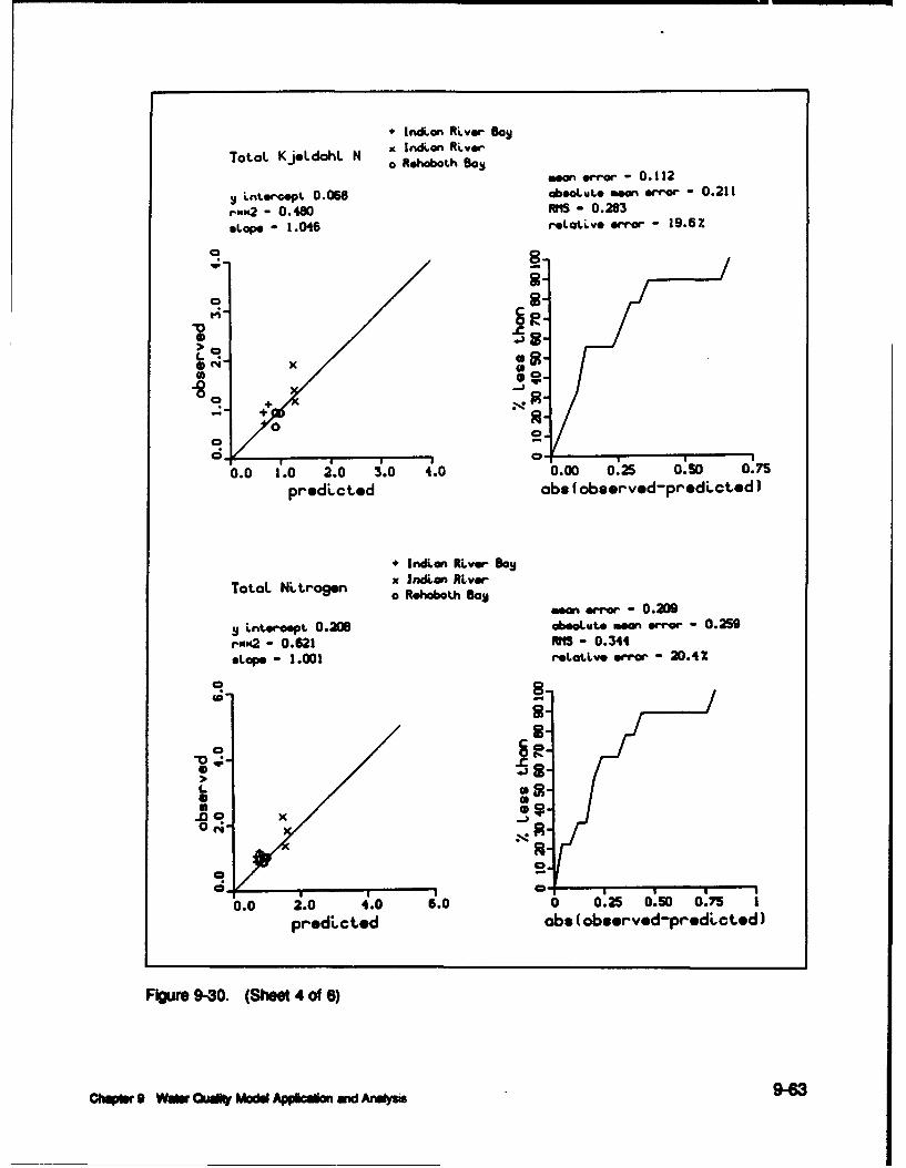
* IrdLan RLver Bog

TotcLKj*LdhL N x IndLon RLverTota Kj.dai~ N 0 Rehoboth eBoJ

soo emwo - 0. 112

,V LnLeE-cept. 0.068 eatuoLYL seon err-or - 0.211-mm OASO RPIS - 0. 283

esoe 1.046 e-tat.Lvo error -19.6Z

> B2

00

0.0 11.0 i.0 3'.0 4.0 0.00 0.25 0.50o 0.,75

predicted abs (obsorvod-prodLctod)

* IndLen RLver Bagj

Tota N~togen x JndAon RLVsrTotalNL~r9.n o Rehobo~h Bog

meon error - 0.2D9S Lnt~eiet. 0.208 cbeoLut~e menerror - 0.259,-uu2 -0.621 RM- 0.344*top. 1.001 retLatLv* error -20.4%

40

>B

L

x -

00

0.0 2.0 4.0 6.0 0 0.25 0.'50 0.'75

predLctoed abs (obsorvod-prodLctod)

Figure 9-30. (Sheet 4 Of 6)

Chimplr 9 Was. Oudky Lmadu Appicatan and Analysi 96

* IndLwn RLver Bao

OLesoLvd pnorgonLcy ld*W&*n RLverO~~amo~~ved [•cL Rehoboth Boy

mom error - 0.021

. Lntercept 0.033 &aloLute mwn erro' - 0.021r--2 0.345 0 - 0.022Loape -1.140 reloaLv* error - 79.3Z

-8-

"8 .o

!i X IR

* R_

0.00 0.05 0.10 0.15 0.00 0.02 0.04 0.06predLcted abe (observed-predLcted)

* IndLan RLver BagTotaL Phosphorus In•dLon RLv

oRehoboth Soymom error u- 0.024

s inter-ept. 0.052 abeavut, mean error - 0.025rw2 - 0. 150 MS - 0.035*Lope 0.633 rLotLve error - 25.1Z

CC

L C;_

0.2.

.0 +8

o -

0.0 0.1 0.2 0.3 0.4 0.0000.025 0.050 0.0"5 0.100predLct ed abe (observed-predLcted)


9-64 ChPrW 0 WaMr Quaky MOdM ApOi m d An*Ws

* Indi~an Rt~ver Basi

OLssoLved Oxl9gen x Ind~an RLver* Rehoboth BaSj

.4 Lnteorcept 12.397 ~asotute error .- -t 1.26-am 0.07S RMs - 1.767

*Lope -- 1.007 re~ta.LvoerrWor. 27.4Z

4)

C C

0.0 i. 10.0 1S.0 0 tpI-edLc ted abs (obsorvocedprodLcted)


ChqWr9 Wuir WAY MOMe AppOicOmn md Anlm"W9-6

Modeled temperature was ideal on a point-by-point basis so little additionalinformation was gained by examination of aggregated values. Aggregation ofsalinity, however, indicated nearly perfect model-data agreement for six of nineseasonal-regional averages. Model chlorophyll results were perfect in IndianRiver Bay. The model overestimated chlorophyll in Rehoboth Bay, however.Chlorophyll in upper Indian River was underestimated for reasons previouslyexplained. The behavior of aggregated BOD was the same as for individualcomparisons. The model indicated the correct trend in BOD but underesti-mated concentration. Large portions of the erratic ammonium comparisonswere removed by seasonal-regional averaging. Model-data ammonium com-parisons were ideal for five of nine seasonal-regional combinations. Erraticpredictions and observations still existed for some seasons and regions, how-ever. Nitrate, total Kjeldahl nitrogen, and total nitrogen comparisons on theseasonal-regional basis mirrored the favorable performance of individual com-parisons. Phosphate demonstrated a clear trend of underprediction by themodel in all regions. Total phosphorus demonstrated ideal agreement of pre-dictions and observations in most regions and seasons although the modelunderestimated in some comparisons. Comparisons indicated the model over-estimated dissolved oxygen in most season-region combinations but correspon-dence in several was near-perfect.

Statistical Evaluation

The scatterplots are useful, qualitative summaries of model performance.Quantitative measures are preferred by some analysts, however. No consensusexists on a standard suite of quantitative performance measures. As a result,we compute a large suite, reported on the same figures as the scatterplots(Figures 9-29, 9-30).

Regression Analysis - One popular form of model-data comparison treatsmodel results'as independent variables and observations as dependent variablesin linear regression analysis. A high degree of correspondence between modeland observations is indicated by a correlation coefficient near unity, an inter-cept near zero, and a slope near unity.

Mean Error - The mean error statistic is defined:

ME ( - P) (9-1)n

ME = mean error

0 = observation

P = model result

9-66 Chqr 9 Water Ouality Model Applicea*o id Analysis

n = number of observations

The mean error is a summary of the model tendency to overestimate orunderestimate the data. The mean error can be zero even though large discrep-ancies exist in individual model-data comparisons. The mean error is espe-cially useful to indicate potential errors in loads, sediment-water fluxes, andother sources and sinks to the water column.

Absolute Mean Error - The absolute mean error statistic is defined:

AME 10 [ - P1 (9-2)

n

AME = absolute mean error

The absolute mean error is a measure of the average discrepancy betweenobservations and model results. The absolute mean error does not differentiatebetween overestimates and underestimates by the model.

Root Mean Square Error - The root mean square error statistic is defined:

RMS = ( - p)2 (9-3)

IN n

RMS = root mean square error

The root mean square error is an alternate quantification of the averagediscrepancy between observations and model results.

Relative Error - The relative error is defined:

RE = E - (9-4)

RE = relative error

The relative error statistic normalizes absolute mean error by the magnitudeof the observations. The relative error statistic is especially useful in compar-ing performance between variables of different magnitude or performance ofmodels of different systems.

ChapW 9 waar Ouay ModW Appiwam aid amon 9-67

The mean error and root mean square error for major water quality constit-uems are summarized in Table 9-1. Summaries are for instantaneous and

seasonal-regional comparisons.

TWIb 9-1

SuNINwy of um Nd Root MWe SuM Error

w oor mm wWr - wr_[_Rm Mwor

Sm inWii Piver I , Wn Ikw, nain w, Mn Over,kdwl"o Sarunsr.Rqianl biviid SuMr-RhglWWo

kImN Poins ALyep km Poinfa AverW

Temperature, -0.08 0.84 2.25 1.49Co

Salinity, 2.53 -2.16 5.9 3.46ppt _ _ _ _ _ _ _ _ _ _ _

Chlorophyll, 15.9 29.1 102.3 74.1mg __ _ __-_ _ _ _ __ _ _ _

BOOS, 141 2.37 1.85 2.37gm m-1

Ammonium, -0.016 0.029 0.145 0.115gm m-

Nitrate, -0.037 0.102 0.338 0.111gm m-

Total Kjeldahl 0.055 0.112 0453 0.283N, gm m-3

Total N, 0.03 0.209 0487 0.344gm m-_

Phophteo, 0.01 0.021 0.048 0.022gm m-_

Total P. 0.019 0.024 0.061 0.035gm m-_

Dissolved -141 -1.22 2.75 1.77Oxygengm M-_

The summary indicates mean error is generally larger in magnitude for thesummer average tha= for individual observations. One interpretation of thisphenomenon is that sources and sinks for summer only are quantified to alesser degree of accuracy than for the time period encompassed by the entiredata base (April through September). The RMS error for the seasonal-regionalaverage is about half the error for instan eous comparisons. The implicationof this statistic is that the model is more accurate in reproducing spatial andtemporal aggregations than individual observations.

9-68 ChepWv 9 wAW Ouf Made Ap a~m &WAnaby

Interpretation of performance statistics is facilitated when some basis forcomparison is present. We compared the relative error statistics with results ofthe Chesapeake Bay model study (Cerco and Cole 1993). Individual and sea-sonal-regional averages from Indian River were compared to seasonal-regionalaverages from the Bay (Figure 9-31). The Chesapeake Bay study made use ofan extensive, high-quality data base and employed highly accurate measures ofloads and boundary conditions. Calibration of the model consumed severalyears and was subject to extensive review. We regard the performance statis-tics of the Bay study as current state of the art for long-term applications ofcomprehensive eutrophication models.

Relative error for seasonal-regional averages in the Indian River modelapplication was generally greater than in Chesapeake Bay but comparable forall but two substances. Relative error for chlorophyll in Indian River wasdouble the Chesapeake Bay value. The chlorophyll statistic in Indian Riverreflected the extreme concentrations observed at the surface near the Millsborospillway. Concentrations in excess of 1000 mg m3 were in the data base.Discrepancies between these observations and model results added enormousbias to the performance statistics. Relative error for phosphate was also doublethe Chesapeake Bay value. We were informed by DNREC that the phosphatedata in STORET is dubious. We noted the STORET phosphate data fre-quently disagreed with the observations collected by the College of MarineStudies (Figures 9-3, 9-4, 9-7, 9-8). Most often, when conflicts in the datawere noted, model results conformed to the College of Marine Studies ratherthan the STORET data. We concluded the large phosphate relative error wasdue to faulty data rather than a shortcoming in the model calibration.

The Annual Cycle of Water Quality

The time series of conditions in the water column, sediment-water interac-tions, and interpretive quantities, together with other information availablefrom the model permit a description of the annual cycle of water quality inIndian River/Rehoboth Bay.

During the first four months of the year, chlorophyll is virtually absentfrom the water column (Figures 9-2 through 9-9). Nitrogen, in the form ofnitrate, and light to support algal growth are readily available (Figures 9-21through 9-28). A slight phosphorus limitation to growth is present but theprimary influence on algal abundaive is temperature. The water is too cold tosupport substantial primary production by phytoplankton. In May, the waterwarms sufficiently to support algal production so that chlorophyll concentra-tion rapidly rises to its summer maximum value. Limitations to algal growthduring summer vary. Light extinction, due to background extinction and algal-self shading, is at its annual peak (Figures 9-21 through 9-28). In upperIndian River, phosphorus is the limiting nutrient (Figures 9-21 through 9-23).In Lower Indian River and in Rehoboth Bay, however, nitrogen is the domi-nant nutrient limit on algal growth (Figures 9-24 through 9-28). Chlorophyllconcentration fluctuates, in response to flow and loading events, until

Chapler 9 Water Ouay Mode Appklio and Anais 9-69

d mjlS

ii*uqdolqj IAmps

7.Uadm

0 14ccI ~r *1u

'I I.

Chp WAW Ouao tII' Apam&WAd

mid-October. In October, temperature falls below the level needed to supportsubstantial algal growth and chlorophyll declines to its winter minimumconcentration.

During the first four months of the year, background light extinction is nearits minimum value and light attenuation by chlorophyll is negligible (Fig-ures 9-21 through 9-28). Light is available to support production by benthicalgae. As a consequence, dissolved oxygen is produced at the sediment-waterinterface and released to the water column (Figures 9-13 through 9-20).Ammonium and phosphate are removed from the water column and consumedat the sediment-water interface. Nitrate transport is into the sediments, drivenby the high concentrations in the overlying water. Two phenomenon accom-pany the wanning of the water column in May. First, oxygen consumptionand nutrient production in the subsurface sediments increase. Second, lightextinction increases due to the seasonal variation in background extinction andchlorophyll attenuation. As a consequence of temperature-enhanced sedimentprocesses and shading of the benthic algae, the sediments consume oxygenremoved from the water column. The sediments become sources of ammon-ium and phosphate to the water. Sediment-water nitrate flux is negligible dueto diminished concentration in the overlying water. Sediment consumption ofoxygen and production of ammonium and phosphate continue until autumncooling of the water column. Cooling diminishes diagenetic processes in thesediments and is accompanied by diminished light extinction. Benthic algaebecome active so that, by the end of the year, dissolved oxygen is again pro-duced at the sediment-water interface. Ammonium and phosphate enter atransition from sediment release to consumption at the sediment-water inter-face.

The annual nitrogen cycle varies according to location. In lower IndianRiver and Rehoboth Bay (Figures 9-5 through 9-9), total nitrogen concentra-tion demonstrates a sinusoidal behavior with maximum concentration in latesummer. The phase of the total nitrogen function corresponds to the phase ofannual temperature variation. The correspondence occurs because temperaturedrives sediment ammonium release (Figures 9-13 through 9-20), a primarysource of nitrogen to the lower Bays. In upper Indian River, total nitrogen ismore closely related to runoff events so that maximum concentrations typicallyoccur in late winter or early spring (Figures 9-2 through 9-4). Since nitrate isa major constituent of runoff nitrogen, nitrate maxima occur in winter andspring throughout the system. The magnitude of the maximum diminishesaway from the runoff entry points, however. In the lower Bays, in summer,nitrate is virtually absent due to algal uptake and negligible local runoff. Theammonium cycle is complex, influenced by external loading, sedimentproduction/consumption, and algal uptake. In much of the system, a summermaximum, coincident with sediment release would be expected. As rapidly asammonium is released from the sediment, however, it is consumed by algae.In lower Indian River and Rehoboth Bay (Figures 9-5 through 9-9) maximumammonium concentrations are evident in October through December. In thesemonths, phytoplankton uptake is diminished but uptake by benthic algae is notsufficient to remove the ammonium from the water column. Upper Indian

Chb 9 WAt Oudy Model Apcow mad Amlysm 9-71

River also demonstrates the autumn peak but high concentrations, due to sedi-ment release, occur in summer as well. In this portion of the system, summeralgae populations tend to be limited by phosphorus availability so that not allammonium is removed by algal activity.

The annual cycle of total phosphorus also coincides with the temperaturecycle. As with nitrogen, the coincidence is due to temperature-enhanced nutri-ent release from the sediment. The influence of runoff in the annual phospho-rus cycle is not as evident as for nitrogen however (Figures 9-2 through 9-4).Annual cycling in phosphate is similar to ammonium. Lower Indian River andRehoboth Bay demonstrate an autumn peak (Figures 9-5 through 9-9) thatpresumably is due to diminished phytoplankton uptake coupled with minimalactivity by benthic algae. Near the Millsboro spillway, however, phosphateexhibits erratic behavior due to loading from runoff events, consumption andrelease in sediments, and algal uptake.

As with most estuarine systems, minimum dissolved oxygen in IndianRiver/Rehoboth Bay occurs during late summer when water temperature ishighest. The coincidence of high temperature and low dissolved oxygen is dueto temperature-enhanced respiration in the water and sediments and due todiminished saturation dissolved oxygen concentration. Conversely, anmualpeaks in dissolved oxygen occur in winter when low temperature diminishesrespiration in the water column, light stimulates benthic algal production, andsaturation concentration is maximum. Our model indicates minimum daily-average dissolved oxygen concentrations of 2 to 3 gm m3 occur in upperIndian River (Figures 9-2, 9-3). In lower Indian River and Rehoboth Bay, wetypically indicate minimum daily-average dissolved oxygen concentrations of6 gm m-3 (Figures 9-5 to 9-9). Observations indicate virtually no dissolvedoxygen concentrations below 2 gm m-3. In lower Indian River and RehobothBay, however, a substantial proportion of observations fall below our 6 gm m-3

minimum. A portion of the discrepancy lies in the problem of comparing grabsamples with daily average model output, as previously described. Severalaspects of the comparisons remain problematic, however. Observations atmost stations indicate dissolved oxygen was lower in 1989 and 1990 than in1988 (Figures 9-4 through 9-9). We cannot explain this phenomenon; ourmodel indicates dissolved oxygen is equivalent in the three summers. Ourmodel also agrees well with the summer 1988 observations. Observations atmost stations indicate minimum dissolved oxygen in 1990 occurred at thebeginning of May, at a water column temperature less than 10 C0, rather thanlater in the year. We believe the data base merits careful examination beforeconclusions are drawn regarding the ability of the model to reproduce theannual cycle of dissolved oxygen.

A mass-balance feature of the model allows computation of internal mater-ial sources and sinks. These are compared with the external loads quantifiedearlier (Chapter 3). On an annual basis, nonpoint sources are the largest nitro-gen loads to the Indian River/Rehoboth Bay system (Figures 9-32 through9-34). Atmospheric loads are the second largest source while point sources arethe least of the sources quantified. Most of the nitrogen load to the system is

9-72 Chapter 9 Wier Quality Model Appicalin ard Analysis

1988

NITROGEN

-49.sE SEDIMENTS7•65. 3 ATMOSPHERE

POINT SOURCE_J1282.1 NONPOINT SOURCE

- 1817.0 V_///__///_ OCEAN EXCHANGE

-3500 -1750 01750 3500kg/DAY

PHOSPHORUS

-157.0o SEDIMENTS0.0R ATMOSPHERE

2n POINT SOURCE47.9 NONPOINT SOURCE

81.4 OCEAN EXCHANGE

-200 -100 0 100 200kg/DAY

CARBON

'-9610.7 ///SEDIMENTS777= 25•.7 PRIMARY PRODUCTION

POINT SOURCENONPOINT SOURCE

-249.9__ OCEAN EXCHANGE

-1500 -750 0 750 15000kg/DAY

Figure 9-32. Annual Mass Balance, 1988

chmpW WAIr QiUdy MOM u d Aplcu•mn wd Auus 9-73

1989

NITROGEN

-810.9 - EDI MENTS• "'I765.3 ATMOSPHERE

T .3 POINT SOURCE011"/////7I,5 7 8 NONPOINT SOURCE

-2610.4 [/// //,• "" ' "OCEAN EXCHANGEI I I

-3500 -1750 0 1750 3500kg/DAY

PHOSPHORUS

-174.e[ / // / // S DI MENTS-017.. A MOSPHERE02.6 POINT SOURCE

125.5 NONPOINT SOURCEYJ29.5 OCEAN EXCHANGE

-200 -100 0 100 200k9/DAY

CARBON

-1164.4 • SIMENTSI9Mj.3 PRIMARY PRODUCT IONPOINT SOURCE

2I0047.4 NONPOINT SOURCE-73S2.9 OCEAN EXCHANGE

-1= -750 0 7500 15000kg/DAY

Figure 9-33. Annual Mass Balance. 1989

9-74 Chvap 9 WAsr Oudy ModW Apo•com W Anus

1990

NITROGEN

-83.2 SED I MENTS765.3 ATMOSPHERE165.6 POINT SOURCE

7777 / . NONPOINT SOURCE-194.51 OCEAN EXCHANGE

-3500 -1750 0 17'50 3500kg/DAY

PHOSPHORUS

-183.9 SEDIMENTS0.0 ATMOSPHERE7J2L.35 POINT SOURCE

74.1 NONPOINT SOURCE"9.1 • OCEAN EXCHANGE

-200 -100 0 100 200kg/DAY

CARBON

-10755.V3 SEDIMENTS111S.0 PRIMA'RRY PRODUCTIONPOINT SOURCE

// 6144.8 NONPOINT SOURCE-4138.3 . OCEAN EXCHANGE

-15000 -7;00 0 150 5000kg/DAY

Figure 9-34. Annual Mass Balance, 1990

chaptr 0 Wamr Quaity Model Apicallan ,Ashm" 9-75

lost through the mouth to the ocean. The remainder is lost to the sedimentswhere it is buried or denitrified to gaseous form.

During years of dry and normal hydrology, the largest source of phosphorusto Indian River/Rehoboth Bay is import through the inlet from the ocean (Fig-ures 9-32, 9-34). In extremely wet years, however, nonpoint- source loadsexceed import from the ocean (Figure 9-33). Point source loads are less thanthe oceanic import or nonpoint sources. No atmospheric load is thought toexist. The sediments represent the only phosphorus sink. Since no processanalogous to denitrification exists for phosphorus, the ultimate sink is burial todeep, inactive sediments.

During years of dry and normal hydrology, the largest source of carbon toIndian River/Rehoboth Bay is primary production by algae (Figures 9-32,9-34). The carbon produced by algae is oxidized in the water column, asBOD, or in the sediments, as sediment oxygen demand. In a wet year, how-ever, a surprisingly large amount of carbon enters from nonpoint sources sothat nonpoint-sources comprise the largest fraction of oxygen demand (Fig-ure 9-33). Point-source carbon loads are negligibly small. Most of the carbonload to the system settles to the sediments where it is oxidized, producingsediment oxygen demand, or buried to deep, inactive sediments. A lesserfraction of the carbon load is exported through the mouth to the ocean.

Summer-Average Water Quality

Spatial representations of water quality (Figures 9-35 through 9-44) wereobtained by averaging model results for June, July, and August 1990, an aver-age hydrologic year. Summer was selected for spatial representation since it isthe season in which water quality problems most often occur.

The model indicates chlorophyll (Figure 9-36) is maximum near the Mills-boro spillway. High chlorophyll concentrations also occur in the headwatersof other major branches. Chlorophyll generally declines away from runoffsources and is least near the Indian River inlet. The chlorophyll distribution isgoverned by the distributions of ammonium (Figure 9-38), nitrate (Fig-ure 9-39), and dissolved phosphate (Figure 9-42). Nitrate and ammonium areabundant, relative to the half-saturation concentration for nitrogen uptake(Table 6-2), throughout most of Indian River. In Rehoboth Bay and IndianRiver Bay, however, nitrate and ammonium are nearly depleted. The spatialdistribution of nitrate reflects the source in runoff and wasteloading and thesink in the ocean. The ammonium distribution indicates a major source issediment release. Dissolved phosphate is maximum in the inlet, indicatingconcentraion in this region is stongly influenced by the ocean boundary con-dition. Phosphate is also high near Millsboro and the Rehoboth Beach outfall.Minimum phosphate concentrations occur midway between the inlet and Mills-boro and in portions of Rehoboth Bay. The high chlorophyll levels in upper

9-76 c~ap 9WA w uef 1-1/od ppr~m: aid Aretpi

C - Cia q~ Itde i'tu

do=%

Chopu~r 0 Wow OudIV' tLI.M Appksaim &L Anmlyui 9-77

acCLC? (E

0.*

9-78 ChwWr 0 W*. Qm Mo omdd m DI w~ ujwid nly

_u Cywi a N N464

Lo~ $JT .7' -

a~l E0 E,

Caioswr9 Woo Qudly MPMd Applcoala um An**ui 9-79

0OD 4 dId 40 osd I 0ccddcoo

E

9-M WW 9WaW wftMoM poc~ wW n~E

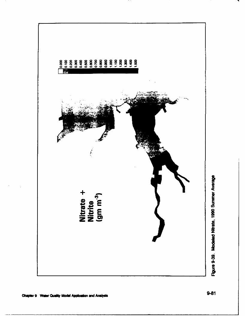
am &Mz

ChmpW~ 9 amQ_ o pl~ WA~b98

-mI- EI

9-82 Oh~~~Sr 9 WE"a Quft mome 40pcoonmd Anelyinj

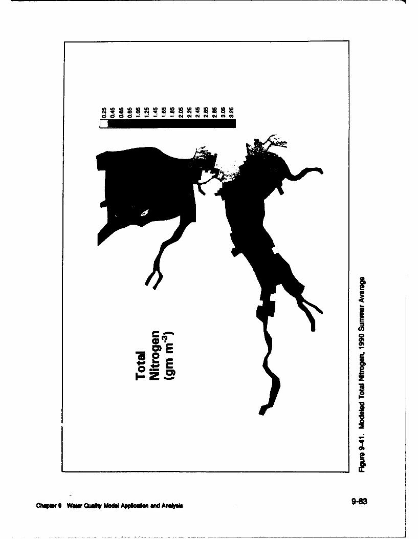
0 00 ~ - -- C4 cm Cli cm C4 V0 M

I-2~ z

ChmW sr WArn Ou*l Modi Apoadan &Wd An~iftu~ 9-83

ddoddo dooododcio

C,0 e

CA cl)

U.

9-M~ 2~pr a~mt mmA)k~#~wj

'4 11

eon%

a E

iE

ChpW9 a QftM" po~m& A*) i

..... ....

* * ** * * * er- r- ,- #. I- t- r- v-

I,'IE

6,

o&E I*� �E I

a

I

II

9-86 Ch�sr 9 Wulir Ou*y Mod� Applodan u�d Anulyuis

Indian River reflect the availability of nitrogen and phosphorus foralgal growth. Phosphorus is the limiting nutrient in this region (Figures 9-21through 9-23). In lower Indian River and Rehoboth Bay, phosphorus is avail-able to support algal growth but nitrogen is limiting (Figures 9-24 through9-28). The transition from phosphorus limitation in headwaters to nitrogenlimitation near the ocean interface is a typical estuarine characteristic.

The distribution of total nitrogen (Figure 9-41) shows clearly the transitionfrom sources along the shore to the sink in the ocean. Total phosphorusexhibits the same trend (Figure 9-43).

Results of the model indicate anoxia is not a permanent feature anywhere inthe system (Figure 9-44). Summer-average dissolved oxygen exceeds 6 gm m3 everywhere. Observations and the model indicate, however, that concentra-tions as low as 2 gm m 3 occur. Excursions below average occur on a diurnalbasis due to algal respiration, and on the time scale of days due to flow eventsand similar phenomenon. Highest dissolved oxygen concentrations coincidewith highest chlorophyll concentrations indicating the role of algal productionin dissolved oxygen production. Minimum dissolved oxygen occurs abouthalfway between Millsboro and Indian River inlet. The origin of the minimumis not apparent but chlorophyll is also low in this region suggesting the mini-mum is due to limited algal production.

A substantial and significant difference exists between annual mass balances(Figures 9-32 through 9-34) and summer-average mass balances (Figures 9-45through 9-47). During summers of dry and normal hydrology (Figures 9-45,9-47) sediments are the largest nitrogen source to the system, through themechanism of ammonium release. Even in an extremely wet summer, sedi-ments rival nonpoint sources of nitrogen (Figure 9-46). The summer massbalance contrasts with the annual balance in which sediments are a net nitro-gen sink. A similar balance exists for phosphorus. The sediment release ofphosphorus is sufficient to convert the system into a net exporter of total phos-phorus during the summer. By contrast, on an annual basis, the sediments area phosphorus sink and the system imports phosphorus from the ocean. Therole of sediments in summer in Indian River/Rehoboth Bay is consistent withthe role of sediments in larger, deeper estuaries. The net nutrient release insummer is due to two factors. High temperature which enhances diagenetic(decay) processes in the sediments and seasonal turbidity increase whichshades out benthic algae.

Chaplr 9 Water audity Moder Appkabon and Analysis 9-87

Summer1988

NITROGEN

2468.4 SEDIMENTS

S.3a' ATMOSPHERE1994 POINT SOURCE

4W. NONPOINT SOURCE-3745.0 OCEAN EXCHANGE

-7000 -3500 0 3500 7000

kg/DAY

PHOSPHORUS

• 173.4 SEDIMENTS.0e ATMOSPHERE

POINT SOURCEr24.8 NONPOINT SOURCE

.- 208.2 in OCEAN EXCHANGE

-4400 -200 0 200 400kg/DAY

CARBON

-8598.5 =ý EDIMENTS

" 222 /2944.6 APRIMARY PRODUCTION350.0POINT SOURCE

3 2SS.26 NONPOINT SOURCE.13126.7=_ OCEAN EXCHANGE

-50000 -250 0 200 50000kg/DAY

Figure 9-45. Summer Mass Balance, 1988

9-88 ChmwrO Wap.a.; iMoM Apo m wW An*d b

Summer1989

NITROGEN

1917.5 SEDIMENTS

7663S.3 ATMOSPHEREn 179.5 POINT SOURCEv////125W1.0 NONPOINT SOURCE

-5W.377 OCEAN EXCHANGE

-7000 -350 0 3500 7000kg/DAY

PHOSPHORUS

162.9 SED I MENTSATMOSPHERE.0 POINT SOURCE

161.2 NONPOINT SOURCE-309.6 OCEAN EXCHANGE• 400 -40 0 260 400

kg/DAY

CARBON

-23340.6r77= SEDIMENTS

~F7777777J 3506.6PRIMARY PRODUCTION"4. "POINT SOURCE

122M.3 NONPOINT SOURCE-22=.o/ OCEAN EXCHANGE

I I I

-500o -2560 0 2kg/DAY


Chmw9 Wam Qauwy Mocdm Apoplafa maid AaWs

Summer1990

NITROGEN

M•.3,. SRI HII£T

NONPOINT SOURC

-3"3.7 OCEA EXCHANGE-700o -35o 0 3 70

k9/DAY

PHOSPHORUS

• 146.4 SEDI MNTS

.S00 ATMOPHEREPOINT SOURCEsi s NOWP INT SOURCE

-164.0__ OCERN EXCHANGE

-40 -200 0 200 400k9/DAY

CARBON

-21114.4 SEDIENTS!-46.1/ PR I RY PRODUCTIONPOINT SOURCE

NONINT SOURCE-15746.7 OCEN EXCHANGE

-SOOOO -250oo 0 25i=0 5ooookg/DAY


9-90 CWW 9 Wa w Ouiy Model Apoplon wW Any••is

Chapter X: Conclusions andRecommendations

Conclusions

"Hydrodymmic Model Application

The CH3D hydrodynamic model simulated transport in Indian River/Rehoboth Bay for three years: 1988, 1989, and 1990. Two-dimensional depth-average transport was calculated on a grid containing over 2000 cells roughly50 m by 100 m in lateral and longitudinal extent. Integration time step was30 seconds.

Performance of the model was verified by comparison to observed tiderecorls, current measurements, and salinity data. The model reproducedobserved surface levels throughout the system with an accuracy of a few centi-meters. Current measures, concentrated in the passage between Rehoboth Bayand lower Indian River, were also well-repreiented by the model. The pre-dicted spatial salinity distribution compared well with observations collected inthree independent surveys.

Computation of transport in Indian River/Rehoboth Bay represents thecurrent state of the art in this field. The transport computations are entirelysuited for use in a euuophication model of the system.

Wear Quality Model Application

The water quality model was applied in a continuous mode to simulateconditions in Indian RiveriRehoboth Bay for the years 1988-1990. Transportfor water quality simulation was provided by the CH3D hydrodynamic model.Other water-quality forcing functions included nonpoint-source loading ofnutrients and organic mater, point-source loading of nutrients ,ukl organicmatter, atmospheric nutrient loading, sediment-watr nutrient and oxygenexchanges, oceanic material exchanges, and seasonal light attenuatio. Quani-fication of loads and other forcing functions was performed specifically forthis study and employed the most recent available information. The model

Chapew 10 C~ki* mW Pam-m-mfma10-1

provided a consistent representation of water quality throughout the systemthroughout the year.

The water quality model operated on a tempeaJ icale of -300 seconds anda spatial scale of -500 m. Forcing functions were iu:t resolved on thesescales, however. Consequently, comparisons of model results with observa-tions were more favorable when model and observations were temporally andspatially aggregated. Performance statistics for the Indian River/Rehoboth Baymodel application were nearly at the state of the art for most substances simu-lated. Unfavorable statistics noted for two substances were attributed tounique, highly-localized conditions and to dubious observations.

The model package is entirely suitable for employment to meet the objec-tives stated at the initiation of the project. Existing point-source and nonpoint-source loads are quantified and located throughout the system. These can beadjusted to develop total maximum daily loads for nutrients and organic mat-ter. Diurnal dissolved oxygen variations are obtained by a process that quanti-fies diurnal range as a function of predicted daily-average dissolved oxygenand chlorophyll concentrations.

Recommendations

Application to the existing model package to the existing data base is opti-mal. No improvement of model-data agreement is possible without collectionof additional data. Representation of the system cannot be improved withoutrevisions to the model formulations. Suggested improvements to the data baseand the model follow.

Data Collection

Water-column observations should be collected at consistent locations inIndian River/Rehoboth Bay and at consistent depths. The collection of surfacesamples only should be replaced with a procedure that provides samples repre-sentative of the entire water column. A recommended protocol is to collectsamples at mid-depth when depth is less than 1 m. Collect surface and bottomsamples in water of depth between I and 2 m. Collect surface, mid-depth, andbottom samples in water of depth greater than 2 m. Salinity, temperature, anddissolved oxygen are low-cost measures, often observed in situ. These can bemeasured at multiple depths easily. If resources for analysis are limited, sam-ples of nutrients and organic matter can be composited into one.depth-averagesample prior to analysis.

The existing data base is highly biased towards the months April throughSeptember. While these are the months in which water quality problems aremost severe, lack of observations in the remaining months limits analyses thatmight relate summer water quality conditions to phenomenon that occur in

10-2 Chaqur 10 Conckusion and RscommenWW,

colder months, for example load events or winter diatom blooms. Regularsampling throughout the calendar year is recommended.

The BOD5 observations currently collected are no longer favored as acomponent of long-term estuarine data bases. Neither is BOD a state variablein state-of-the-art eutrophication models. The BOD observation should bereplaced or supplemented with observations of total organic carbon. The totalorganic carbon analyses are necessary in observations of point-source andnonpoint-source loads as well as the water-column. Direct analysis of particu-late and dissolved organic carbon fractions will greatly facilitate future modelapplications.

The detection levels of ammonium, nitrate, and phosphate in the STORETdata base, 1988-1990, are unsuited for the levels of these nutrients often foundin Indian River/Rehoboth Bay. A large fraction of the observations are belowdetection level. Much improved detection levels are possible, as demonstratedin the College of Marine Studies data base.

Light extinction greatly affects water quality in Indian River/Rehoboth Bay.The existing data base, however is assembled from observations of disk visibil-ity (secchi depth). The conversion of disk visibility to extinction relies on anapproximate conversion. Moreover, we found the disk visibility observationsin the STORET data base to be so unreliable we could not use them. Direct,in-situ, measurement of extinction with a photometer or similar insruument isrecommended.

The present program of sediment-water nutrient and oxygen flux measuresshould be continued. Measures should be collected at several times throughoutthe year. Concurrent with the flux measures, water-column light extinctionand light intensity at the sediment-water interface should be recorded. In viewof the role of benthic algae, chlorophyll measurements in surficial sedimentsshould be added to the sampling program.

Mechanistic Sediment Model

One component of the Chesapeake Bay model package applied to IndianRiver/Rehoboth Bay was a mechanistic, predictive model of sediment-waternutrient and oxygen exchanges. Employment of the benthic sediment modelwas discontinued, however, since it did not account for activity of benthicalgae noted in Indian River. The mechanistic model was replaced with empiri-cal models calibrated to available observations. The empirical modelsperformed well in relating existing fluxes to existing conditions, primarilytemperature and light. Inherent in the empirical models, however, was theassumption that basic fluxes wiU not be altered as a result of managementactivities. The empirical models also related sediment-water fluxes to ambientconditions only. The models did not relate summer nutrient fluxes to loads orbenthic algal blooms that occurred the previous winter. Reactivation of themechanistic sediment model is recommended. In order to employ the model,

ch 10oo m a •Fw:mnwdam 10-3

however, it must be modified to account for the effects of benthic algae. Areasonable starting point for the modifications is adaptation to benthic algae ofexisting kinetics formulations that represent water-column phytoplankton.

Multi-Layer Hydrodyrnmlc Model

The data base for Indian River/Rehoboth Bay provided little information onvertical variations in water quality. Most observations were surface only.Examination of limited available observations, collected in Indian River (Tyler1989), indicated vertical variations in temperature, salinity, and dissolved oxy-gen were small, typically less than 1 CO for temperature, 1.5 ppt for salinity,and 0.15 gm m 3 for dissolved oxygen. No distinct pyncnoline was evidentand bottom-water anoxia was absent. Representation of water quality condi-tions in Indian River/Rehoboth Bay did not require a multi-layer model.

The slight salinity stratification suggests, however, that classic density-driven circulation exists, to some extent, in the reach from Millsboro spillwayto the Indian River inlet. The density-driven circulation is superimposed onthe twice-daily flow reversals induced by tides and is characterized by netmotion downstream near the surface and upstream near the bottom. Thestrength of the circulation depends on runoff volume and salinity at the inlet.The density-driven circulation is subject to alteration by local wind conditions.At present, effects of multi-layer circulation, to the extent that they exist, arerepresented by a dispersion term in the mass-transport equation. This repre-sentation is adequate, as evidenced by agreement in modeled and observedsalinity at most locations and times. Still, some improvement in modeledcirculation may be expected by employment of a multi-layer model. In viewof the shallow depth in Indian River/Rehoboth Bay, two layers would suffice.No multi-layer modeling can be conducted, however, until an extensive database of vertical salinity and temperature observations is assembled. Long-termcurrent measures at several locations in the vertical are also desirable.

10-4 ChWr 10 Condusin Amemnwod

References

Academy of Natural Sciences. (1988). "Phytoplankton, nutrients, macroalgaeand submerged aquatic vegetation in Delaware's Inland Bays," BenedictEstuarine Research Laboratory, Benedict. MD.

American Society of Civil Engineers. (1961). "Effect of water temperature onstream reaeration," Journal of the Sanitary Engineering Division, 87(SA6),59-71.

Ammerman, J., and Azam, F. (1985). "Bacterial 5'-nucleodase in aquaticecosystems: a novel mechanism of phosphorus regeneration," Science, 227,1338-1340.

Anders, F. J., Lillycrop, W. J., and Gebert, J. (1990). "Effects of natural andman-made changes at Indian River Inlet, Delaware," Proceedings of theThird Annual National Beach Preservation Technology Conference,St. Petersburg, FL pp 280-294.

Andres, A. S. (1992). "Estimate of nitrate flux to Rehoboth and Indian RiverBays, Delaware, through direct discharge of groundwater," Open FileReport No. 35, Delaware Geological Survey, University of Delaware,Newark, DE.

Biggs, R. B. (1984). "Ambient dissolved oxygen concentrations in DelawareInland Bays," College of Marine Studies, University of Delaware, Newark,DE.

Bird, D., and Kalff, J. (1984). "Empirical relationships between bacterialabundance and chlorophyll concentration in fresh and marine waters,"Canadian Journal of Fisheries and Aquatc Science, 41, 1015-1023.

Boni, L., Caipene, E., Wynme, D., and Redi, M. (1989). "Alkaline phospha-trse activity in Protozonvaulax Tamarensis' Journal of Plankton Research,11, 879-885.

b Ref-1

Cerco, C. F., and Cole, T. (1993). "Application of the three-dimensionaleutrophication model CE-QUAL-ICM to Chesapeake Bay," draft report inrevision, U.S. Army Engineer Waterways Experiment Station, Vicksburg,MS.

Chrost, R., and Overbeck, J. (1987). "Kinetics of alkaline phosphatase activ-ity and phosphorus availability for phytoplankton and bacterioplankton inLake Plubsee (North German eutrophic lake)," Microbial Ecology, 13, 229-248.

Cole, J., Findlay, S., and Pace, M. (1988). "Bacterial production in fresh andsaltwater ecosystems: a cross-system overview," Marine Ecology ProgressSeries, 43, 1-10.

DiToro, D. (1980). "Applicability of cellular equilibrium and Monod theoryto phytoplankton growth kinetics," Ecological Modelling, 8, 201-218.

DiToro, D., O'Connor, D., and Thomann, R. (1971). "A dynamic model ofthe phytoplankton population in the Sacramento-San Joaquin Delta." Non-equilibrium Systems in Water Chemistry. American Chemical Society,Washington, DC, 131-180.

Droop, M. R. (1973). "Some thoughts on nutrient limitation in algae," Jour-nal of Phycology, 9, 264-272.

Edinger, J., Brady, D., and Geyer, J. (1974). "Heat exchange and transport inthe environment," Report 14, Deparlment of Geography and EnvironmentalEngineering, Johns Hopkins University, Baltimore, MD.

Galperin, B., and Mellor, G. L. (1990). "A time-dependent, three-dimensionalmodel of the Delaware Bay and River system. Part 1: Three-dimensionalflow fields and residual circulation," Estuarine, Coastal, and Shelf Science,Vol 31, pp 255-281.

Galperin, B., and Mellor, G. L. (1990). "A time-dependent, three-dimensionalmodel of the Delaware Bay and River system. Part 2: Three-dimensionalflow fields and residual circulation," Estuarine, Coastal, and Shelf Science,Vol 31, pp 255-281.

Gan-att, J. R. (1977). "Review of drag coefficients over oceans andcontinents,'" Monthly Weather Review, Vol 105, pp 915-929.

Genet, L., Smith, D., and Sonnen, M. (1974). "Computer Program Documen-tation for the Dynamic Estuary Model," U.S. Environmental ProtectionAgency, Systems Development Branch, Washington, DC.

Ref-2 RfrWW"M

Johnson, B. H., Heath, R. E., Hsieh, B. B., Kim, K. W., and Butler, H. L.(1991). "User's guide for a three-dimensional numerical hydrodynamic,salinity, and temperature model )f Chesapeake Bay." TechnicalReport HL-91-20, U.S. Army Engineer Waterways Experiment Station,Hydraulics Laboratory, Vicksburg, MS.

Johnston, R. H. (1976). "Relation of ground water to surface water in foursmall basins of the Delaware coastal plain," Report of Investigations No.24, Delaware Geological Survey, University of Delaware, Newark, DE.

Karpas, R. M. (1978). "The hydrography of Indian River and Rehoboth --Delaware's small bays," Master's thesis, University of Delaware, Newark,DE.

Kremer, J., and Nixon, S. (1978). "Light acclimation and the selection oflopt." A Coastal Marine Ecosystem Simulation and Analysis. SpringerVerlag, New York, NY.

Leonard, B. (1979). "A stable and accurate convection modeling procedurebased on quadratic upstream interpolation," Computer Methods in AppliedMechanics and Engineering 19, 59-98.

Lillycrop, W. J., Anders, F. J., McGehee, D. D., Raney, D. C., Gebert, J.,Chasten, M. A., and Welp, T. L. (1991). "Indian River Inlet, Delaware,scour study," Technical Report CERC 91- , U.S. Army Engineer Water-ways Experiment Station, Coastal Engineering Research Center, Vicksburg,MS.

Mark, D. J., Scheffner, N. W., Butler, H. L., Bunch, B. W., and Dortch, M. S.(1993). "Hydrodynamic and water quality modeling of Lower Green Bay,Wisconsin," Technical Report CERC 93-16 , U.S. Army Engineer Water-ways Experiment Station, Coastal Engineering Research Center, Vicksburg,MS.

Matavulj, M., and Flint, K. (1987). "A model for acid and alkaline phospha-tase activity in a small pond," Microbial Ecology, 13, 141-158.

Monod, J. (1949). "The growth of bacterial cultures," Annual Review ofMicrobiology, 3, 371-394.

Morel F. (1983). "Effects of biological processes on pH and alkalinity."Principles of Aquatic Chemistry. John Wiley and Sons, New York, NY,149-151.

Nielsen, P. (1990). "Tidal dynamics of the water table in beaches," WaterResources Research, Vol 26, No 9, pp 2127-2134.

Ref-3

O'Connor, D. (1983). "Wind effects on gas-liquid transfer coefficients,"Journal of the Environmental Engineering Division, 190, 731-752.

O'Connor, D., and Dobbins, W. (1958). "Mechanisms of reaeration in naturalstreams," Transactions of the American Society of Civil Engineers, 123,641-666.

Odum, E. (1971). "Principles pertaining •o limiting factors." Fundamentalsof Ecology. W. B. Saunders, Philadelphia, PA, 106-107.

Parsons, T., Takahashi, M., and Hargrave, B. (1984). Biological oceano-graphic processes. Pergamon Press, Oxford.

Putrevu, U., and Trowbridge, J. (1987). "Numerical simulation of hydrody-namic circulation in Indian River and Rehoboth Bays," Report to DelawareDNREC by University of Delaware, Newark, DE.

Raney, D. C., Doughty, J. 0., and Livings, J. (1990). 'Tidal prism numericalmodel investigation and risk analysis of the Indian River Inlet scour study,"Bureau of Engineering Research, Report No. 500-183, Tuscaloosa, AL.

Redfield, A., Ketchum, B., and Richards, F. (1966). "The influence of organ-isms on the composition of sea-water." The sea vol. ff. Interscience Publi-shers, New York, NY, 26-48.

Ritter, W. F. (1986). "Nutrient budgets for the Inland Bays", FPR-86-001,Agricultural Engineering Department, University of Delaware, Newark, DE.

Roache, P. J. (1976). Computational Fluid Dynamics, Hermosa Publishers,Albuerque, NM.

Sheng, Y. P. (1986). "A three-dimensional mathematical model of coastal,estuarine and lake currents using boundary fitted grid." Report No. 585,A.R.A.P. Group Titan Systems, New Jersey, Princeton, NJ.

Smith, R. 1976). "Longitudinal dispersion of a buoyant contaminant in ashallow channel," Journal of Fluid Mechanics, Part 4, 677-688.

Smullen, J. (1992). "Water quality of Inland Bays," Roy F. Weston Inc.,West Chester, PA.

Steele, J. (1962). "Environmental control of photosynthesis in the sea," Lim-nology and Oceanography, 7, 137-150.

Stumm, W., and Morgan, J. J. (1981). "Oxidation and reduction." Aquaticchemistry. John Wiley & Sons, New York.

Ref-4

Talley, J. H., and Simmons, R. H. (1988). "Inland bays low-flow monitoringJuly 1985 - September 1988," Prepared for Delaware DNREC by DelawareGeological Survey and U. S. Geological Survey.

Thomann, R., and Fitzpatrick, J. (1982). "Calibration and verification of amathematical model of the eutrophication of the Potomac Estuary," Hydro-Qual Inc., Mahwah, NJ.

Thompson, J. F., Warsi, Z. U. A., Mastin, C. W. (1985). Numerical GridGeneration Foundations and Applications, Elsevier Science, New York.

Tchobanoglous, G., and Schroeder, E. D. (1985). "Chemical characteristics ofwater, organic matter." Water quality. Addison-Wesley, Reading, MA,120-121.

Tuffey, T., Hunter, J., and Matulewich, V. (1974). "Zones of nitrification,"Water Resources Bulletin, 10, 555-564.

Tyler, M. (1989). "Inland Bays phytoplankton monitoring study 8 Maythrough September 1988: phytoplankton taxonomy and bloom scenariosfinal report," Versar Inc., Columbia, MD.

Wezernak, C., and Gannon, J. (1968). "Evaluation of nitrification instreams," Journal of the Sanitary Engineering Division, 94(SA5), 883-895.

Wen, C., Kao, J., Wang, L., and Liaw, C. (1984). "Effect of salinity onreaeration coefficient of receiving waters," Water Science and Technology,16, 139-154.

Wong, K-C. (1987). "Tidal and subtidal variation in Delaware's inland bays,"Journal of Geophysical Research, Vol 17, pp 413-422.

Wong, K-C., and DiLorenzo, J. (1988). "The response of Delaware's inlandbays to ocean forcing," Journal of Geophysical Research, Vol 93, CIO,pp 12525-12535.

PRonm• Ref-5

I Form ApprovedREPORT DOCUMENTATION PAGE 0MB No. 070,01Qi84

p,*i~~~~~~c ,otngudn o u bein@anointu MOW estimated t a1ea! 1 hOur We r'mOor. WAmnddn the tiMe for reqwa"wungInctiwns :=@dn=gstn data sources

collecti~ ~ ~ ~ ~~~~~~~~~~464"nf of"KN InomtO..cuig 0 edcn htbre oWsigtnMeqatr wms ecorate for Infmtionm Oerioratbw and Repors. 12 Is feoDeasa0ha.1 Iust U04. ! _V~"22M."43oa. &W to the 04.o dagnetand Gudget PaPerwork Reduction Prgc (07044 I) Washntoen. DC 20503.

1. AGENCY USE ONLY (Leave blank) 2. REPORT DATE 3 REPORT TYPE AND DATES COVEREDI May 1994 Final report

4. TITLE AND SUBTITLE 5. FUNDING NUMBERSHydrodynamic and Eutrophication Model Study of Indian Riverand Rehoboth Bay, Delaware

G. AUTHOR(S)Carl F. Cerco, Barry BunchMary A. Cialone, Harry Wang

7. PERFORMING ORGANIZATION NAME(S) AND ADORESS(ES) S. PERFORMING ORGANIATION

U.S. Army Engineer Waterways Experiment StationREOTNMR3909 Halls Ferry Road Technical ReportVicksburg, MS 39180-6199 IEL-94-5

9. SPONSORING /MONITORING AGENCY NAME(S) AND ADDRESS(ES) 10. SPONSORING/ MONITORINGAGENCY REPORT NUMBER

U.S. Environmental Protection Agency, Region Ill,Philadelphia, PA 19107; Delaware Department of NaturalResources and Environmental Control, Dover, DE 19903; U.S. ArmyEngineer District, Philadelphia, Philadelphia, PA 19106-2991

11. SUPPLEMENTARY NOTES

Available from National Technical Information Service, 5285 Port Royal Road, Springfield, VA 22161.

12a. DISTRIBUTION/ AVAILABILITY STATEMENT 12b. DISTRIBUTION CODE

Approved for public release; distribution is unlimited.

13. ABSTRACT (Maximum 200 words)

Indian River and Rehoboth Bay are two shallow bodies that form part of the Delaware Inland Bays system.The Bays are subject to eutrophication problems that accompany agricultural, commercial, and recreational devel-opment in the coastal zone. A hydrodynamic/water quality model package was applied to provide a managementtool to address eutrophication issues in the two Inland Bays.

The CH3D hydrodynamic model simulated transport in Indian River/Rehoboth Bay for 3 years: 1988, 1989,and 1990. Two-dimensional depth-average transport was calculated on a grid containing over 2,000 cells roughly50 by 100 mn in lateral and longitudinal extent. Integration time step was 30 sec. Performance of the model wasverified by comparison to observed tide records, current measurements, and salinity data.

The water quality model was applied in a continuous mode to simulate conditions in Indian River/RehobothBay for the years 1988-1990. Transport for water quality simulation was provided by the CH3D) hydrodynamicmodel. Other water-quality forcing functions included nonpoint-source loading of nutrients and organic matter,point-source loading of nutrients and organic matter, atmospheric nutrient loading, sediment-water nutrient andoxygen exchanges, oceanic material exchanges, and seasonal light attenuation.

(Continued)

14. SUBJECT TERMS 15. NUMBER OF PAGESDelaware Eutrophication Models Rehoboth Bay 262Dissolved oxygen Indian River Nitrogen 16. PRICE CODEEstuaries Inland bays Phosphorus_________

17. SECURITY CLASSIFICATION 18. SECURITY CLASSIFICATION 19. SECURITY CLASSIFICATION 20. LIMITATION OF ABSTRACTOF REPORT j OF THIS PAGE OF ABSTRACT

UNCLASSIFID I UNCLASSIFIED I________NSN 7540-01-280-5500 Standard Form 298 (Rev. 2489)

Prescrie by ANSI Std Z39-16296-102

13. Concluded

Project objectives required a model package suitable for development of total maximum daily loads, point-source waste load allocations, and nonpoint-source load allocations of nutrients and organic substances. Addi-tional requirements were that the model package operate in a continuous multiyear mode and provide informationon diurnal dissolved oxygen variations. The model package was also to provide an organized framework forcollection and employment of additional observations in the study system. The model package described in thisreport is entirely suitable for employment to meet these objectives.

hydrodynamics and eutrophication model study of indian

Documents