hybrid’4d’envar’for’the’ncep’gfs:’’progress’...
TRANSCRIPT

Hybrid 4D EnVar for the NCEP GFS: Progress towards opera>onal implementa>on
Daryl Kleist
1 Central Weather Bureau, Taipei, Taiwan – 5 November 2014
with acknowledgements to Dave Parrish, Jeff Whitaker, John Derber, Russ Treadon, Wan-‐shu Wu, Kayo Ide, and many others
Univ. of Maryland-‐College Park, Dept. of Atmos. & Oceanic Science
Outline
• 3D Hybrid Summary
• 2014 GFS Implementa>on – T1534 L64 Semi-‐Lagrangian GFS – Stochas>c Physics
• 4D-‐Ensemble-‐Var
• Implementa>on plans
2
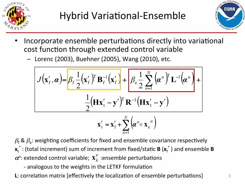
βf & βe: weigh>ng coefficients for fixed and ensemble covariance respec>vely xt’: (total increment) sum of increment from fixed/sta>c B (xf’) and ensemble B αn: extended control variable; :ensemble perturba>ons
-‐ analogous to the weights in the LETKF formula>on L: correla>on matrix [effec>vely the localiza>on of ensemble perturba>ons] 3
Hybrid Varia>onal-‐Ensemble
• Incorporate ensemble perturba>ons directly into varia>onal cost func>on through extended control variable – Lorenc (2003), Buehner (2005), Wang (2010), etc.
ekx
( ) ( ) ( ) ( ) ( )
( ) ( )yxHRyxH
LxBxx
ʹ′−ʹ′ʹ′−ʹ′
++ʹ′ʹ′=ʹ′
−
=
−− ∑
t1T
t
1
1Tef
1f
Tfff
21
21
21 N
n
nnββ,J ααα
( )∑=
+ʹ′=ʹ′N
n
nn
1eft xxx !α

Single Temperature Observa>on
4
3DVAR
βf-1=0.0 βf
-1=0.5

5
EnKF member update
member 2 analysis
high res forecast
GSI Hybrid Ens/Var
high res analysis
member 1 analysis
member 2 forecast
member 1 forecast
recenter analysis ensemble
GDAS Opera>onal Hybrid 3DEnVar
Member N forecast
Member N analysis
Previous Cycle Current Update Cycle
T25L64
T57L64
Generate new ensemble perturbaJons given the latest set of observaJons and first-‐guess ensemble
Ensemble contribuJon to background error
covariance Replace the EnKF
ensemble mean analysis

6
Global Data Assimila>on System Upgrade
• Hybrid system • Most of the impact comes from
this change • Uses ensemble forecasts to
help define background error
• NPP (ATMS) assimilated • Quick use of data aZer launch
• Use of GPSRO Bending Angle rather than refracJvity • Allows use of more data
(especially higher in atmos.) • Small posiJve impacts
• Satellite radiance monitoring code • Allows quicker awareness of
problems (run every cycle) • Monitoring soZware can
automaJcally detect many problems
• Post changes • AddiJonal fields requested
by forecasters (80m variables)
• Partnership between research and operaJons
Implemented 22 May 2012
Opera>onal Configura>on
7
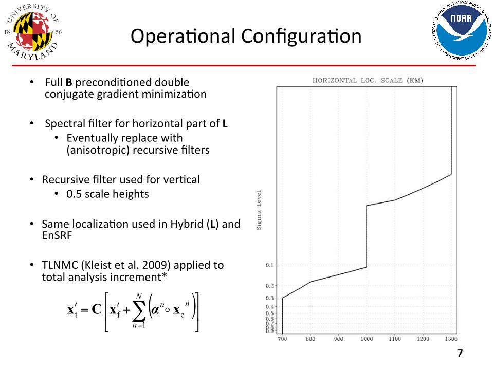
• Full B precondi>oned double conjugate gradient minimiza>on
• Spectral filter for horizontal part of L • Eventually replace with (anisotropic) recursive filters
• Recursive filter used for ver>cal • 0.5 scale heights
• Same localiza>on used in Hybrid (L) and EnSRF
• TLNMC (Kleist et al. 2009) applied to total analysis increment*
7
( )⎥⎦
⎤⎢⎣
⎡+ʹ′=ʹ′ ∑
=
N
n
nn
1eft xxCx !α

Hybrid Impact in Pre-‐implementa>on Tests (to appear in BAMS ar>cle)
8
Figure 01: Percent change in root mean square error from the experimental GFS minus the opera>onal GFS for the period covering 01 February 2012 through 15 May 2012 in the northern hemisphere (green), southern hemisphere (blue), and tropics (red) for selected variables as a func>on of forecast lead >me. The forecast variables include 1000 hPa geopoten>al height (a, b), 500 hPa geopoten>al eight (c, d), 200 hPa vector wind (e, f, h), and 850 vector wind (g). All verifica>on is performed using self-‐analysis. The error bars represent the 95% confidence threshold for a significance test.

Hybrid Impact in Pre-‐implementa>on Tests (to appear in BAMS ar>cle)
9
Figure 02: Mean tropical cyclone track errors (nau>cal miles) covering the 2010 and 2011 hurricane seasons for the opera>onal GFS (black) and experimental GFS including hybrid data assimila>on (red) for the a) Atlan>c basin, b) eastern Pacific basin, and c) western Pacific basin. The number of cases is specified by the blue numbers along the abscissa. Error bars indicate the 5th and 95th percen>les of a resampled block bootstrap distribu>on.

Outline
• 3D Hybrid Summary
• 2014 GFS Implementa>on – T1534 L64 (~13km) Semi-‐Lagrangian GFS – Stochas>c Physics
• 4D-‐Ensemble-‐Var
• Implementa>on plans
10

Implementa>on Overview
• This upgrade is planned for December 9, 2014 • System descrip>on
• This is a change to the GDAS and GFS. • What’s being changed in the system
• Analysis • Model
• T1534 (to 10 days) Semi-‐Lagrangian • Use of high resolu>on daily SST and sea ice analysis • Physics • Land Surface
• Post Processor • Expected benefits to end users associated with upgrade
• Upgrade in global modeling capability. • Improvement in forecast skill
• This implementa>on will put GFS/GDAS into EE process.
11
Analysis Highlights
• Structure • T574 (35 km) analysis for T1534 (13 km) determinis>c • Code op>miza>on
• Observa>ons – GPSRO enhancements – improve quality control – Updates to radiance assimila>on
• Assimilate SSM/IS UPP LAS and MetOp-‐B IASI radiances • CRTM v2.1.3 • New enhanced radiance bias correc>on scheme • Addi>onal satellite wind data – hourly GOES, EUMETSAT
• EnKF modificaJons – StochasJc physics in ensemble forecast – T574L64 EnKF ensembles
12

Model Highlights (1)
• T1534 Semi-‐Lagrangian (~13 km)
• Use of high resolu>on daily SST and sea ice analysis
• High resolu>on un>l 10 days
• Dynamics and structure upgrades – Hermite interpola>on in the ver>cal to reduce stratospheric
temperature cold bias. – Restructured physics and dynamics restart fields and updated sigio
library – Divergence damping in the stratosphere to reduce noise – Added a tracer fixer for maintaining global column ozone mass – Major effort to make code reproducible
13

Model Highlights (2)
• Physics upgrades – Radia>on modifica>ons -‐-‐ McICA – Reduced drag coefficient at high wind speeds – Hybrid EDMF PBL scheme and TKE dissipa>ve hea>ng – Retuned ice and water cloud conversion rates, background diffusion of momentum and heat, orographic gravity-‐wave forcing and mountain block etc
– Sta>onary convec>ve gravity wave drag – Modified ini>aliza>on to reduce a sharp decrease in cloud water in the first model >me step
– Correct a bug in the condensa>on calcula>on aper the digital filter is applied
14

Model Highlights (3)
• Boundary condi>on input and output upgrades – Consistent diagnosis of snow accumula>on in post and model – Compute and output frozen precipita>on frac>on – New blended snow analysis to reduce reliance on AFWA snow – Changes to treatment of lake ice to remove unfrozen lake in winter
– Land Surface • Replace Bucket soil moisture climatology by CFS/GLDAS • Add the vegeta>on dependence to the ra>o of the thermal and momentum roughness, Fixed a momentum roughness issue
15
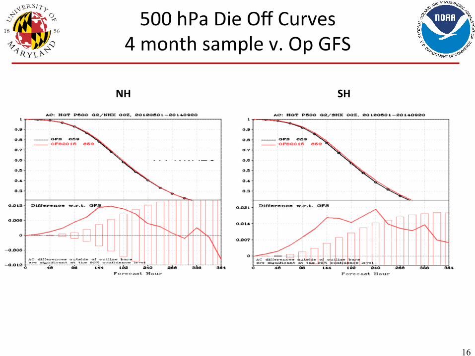
500 hPa Die Off Curves 4 month sample v. Op GFS
16
NH SH

Fit to RAOBS, RMSE Merged 2012/2013/2014
17
Global Mean Temperature RMSE Global Mean Wind RMSE
http://www.emc.ncep.noaa.gov/gmb/wx24fy/vsdb/gfs2015/g2o/index.html

Hurricane Verifica>on 2012/2013/2014
19
Atlantic Track
Atlantic Intensity
Eastern Pacific Track
Eastern Pacific Intensity

Hurricane Verifica>on 2012/2013/2014
20
Western Pacific Track
Western Pacific Intensity
Stochas>c Physics vs Addi>ve Infla>on

22 22
Spread behavior (2014042400)
• Current opera>ons – Spread too large – Spread decays and
recovers
• Stochas>c Physics – Spread decreased
overall (consistent with error es>mates)
– Spread grows through assimila>on window
3HR 6HR 9HR
23
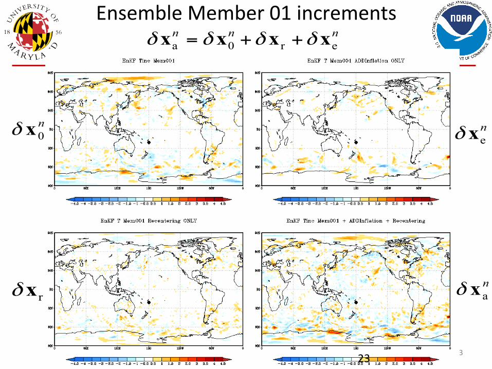
Ensemble Member 01 increments
23
n0xδ n
exδ
rxδnaxδ
nnner0a xxxx δδδδ ++=

Can we replace the addi>ve infla>on by adding stochas>c physics to the model?
• Schemes tested: – SPPT (stochas>cally perturbed physics tendencies – ECWMF tech
memo 598) • Designed to represent the structural uncertainty of parameterized physics.
– SHUM (perturbed boundary layer humidity, based on Tompkins and Berner 2008, DOI: 10.1029/2007JD009284) • Designed to represent influence of sub-‐grid scale humidity variability on the
the triggering of convecHon. – SKEB (stochas>c KE backscaser – also see tech memo 598) – VC (vor>city confinement, based on Sanchez et al 2012, DOI: 10.1002/
qj.1971). Can be determinis>c and/or stochas>c. • Both SKEB and VC aim to represent influence of unresolved or highly damped
scales on resolved scales. • All use stochas>c random pasern generators to generate spa>ally
and temporally correlated noise.
24
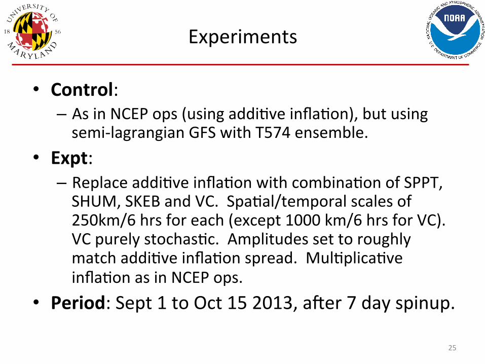
Experiments
• Control: – As in NCEP ops (using addi>ve infla>on), but using semi-‐lagrangian GFS with T574 ensemble.
• Expt: – Replace addi>ve infla>on with combina>on of SPPT, SHUM, SKEB and VC. Spa>al/temporal scales of 250km/6 hrs for each (except 1000 km/6 hrs for VC). VC purely stochas>c. Amplitudes set to roughly match addi>ve infla>on spread. Mul>plica>ve infla>on as in NCEP ops.
• Period: Sept 1 to Oct 15 2013, aper 7 day spinup.
25

6-‐hr forecast spread (zonal wind)
Additive Inflation Stochastic Physics
26
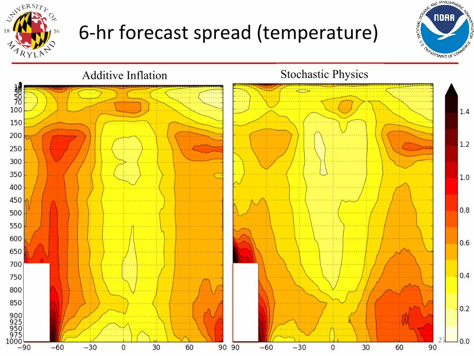
6-‐hr forecast spread (temperature)
Additive Inflation Stochastic Physics
27
28 28
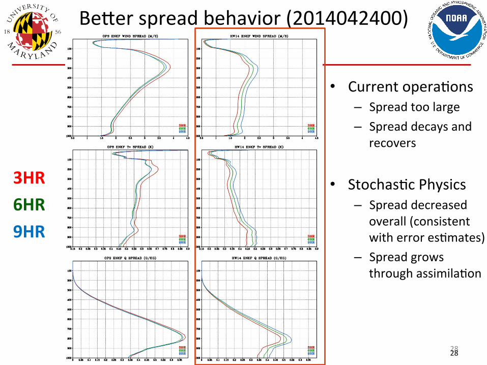
Beser spread behavior (2014042400)
• Current opera>ons – Spread too large – Spread decays and
recovers
• Stochas>c Physics – Spread decreased
overall (consistent with error es>mates)
– Spread grows through assimila>on window
3HR 6HR 9HR

Actual vs Expected O-‐F std. dev. (Vector Wind)
Additive Inflation Stochastic Physics
3386 G. DESROZIERS et al.
In section 2 the general least-variance statistical estimation framework is intro-duced, as well as the consistency diagnostics. A geometrical interpretation of thosediagnostics is given in section 3. An application of the computation of the diagnosticson operational analyses given by a four-dimensional variational (4D-Var) assimilationscheme is presented in section 4. Then, it is shown in section 5 how the diagnosticscan be used to optimize observation and background errors, and an application of sucha tuning algorithm in a simple assimilation toy problem is presented. It is shown insection 6 how such a method can also be used to determine cross-correlations betweenthe errors corresponding to different observations. A spectral interpretation of the diag-nosed covariances is proposed in section 7. Conclusions and perspectives are given insection 8.
2. DIAGNOSTICS IN OBSERVATION SPACE
(a) Consistency diagnostic on innovationsIn statistical linear estimation theory, the expression of the analysed state xa is given
byxa = xb + δxa = xb + Kdo
b,
where xb is the background state, δxa the analysis increment,
K = BHT(HBHT + R)−1
the gain matrix in the analysis process and dob the innovation vector (Talagrand 1997).
The vector dob is the difference between observations yo and their background counter-
parts H(xb), where H is the possibly nonlinear observation operator and H the matrixcorresponding to the linearized version of H . B is the background-error covariancematrix.
From the definition of the innovation vector, the following sequence of relationscan be derived:
dob = yo − H(xb) = yo − H(xt) + H(xt) − H(xb) ≃ ϵo − Hϵb,
where xt is the unknown true state, ϵo the vector of observation errors and ϵb the vectorof background errors. Then, the covariance of innovations is
E[dob(d
ob)
T] = E[ϵo(ϵo)T] + HE[ϵb(ϵb)T]HT,
using the linearity of the statistical expectation operator E, and assuming that observa-tion errors ϵo and background errors ϵb are uncorrelated.
As a consequence, it is easy to check that the relation
E[dob(d
ob)
T] = R + HBHT (1)
should be fulfilled, if the covariance of observation errors, R, and the covariance ofbackground errors in observation space, HBHT, are correctly specified in the analysis.This is a classical result that provides a global check on the specification of thosecovariances (Andersson 2003).
It is shown below how additional relations can be obtained, which provide separatediagnostics on the background-, observation- and analysis-error statistics.
where
obs. error spread
29

Expected vs Actual O-‐F std. dev. (Temp)
Additive Inflation Stochastic Physics
3386 G. DESROZIERS et al.
In section 2 the general least-variance statistical estimation framework is intro-duced, as well as the consistency diagnostics. A geometrical interpretation of thosediagnostics is given in section 3. An application of the computation of the diagnosticson operational analyses given by a four-dimensional variational (4D-Var) assimilationscheme is presented in section 4. Then, it is shown in section 5 how the diagnosticscan be used to optimize observation and background errors, and an application of sucha tuning algorithm in a simple assimilation toy problem is presented. It is shown insection 6 how such a method can also be used to determine cross-correlations betweenthe errors corresponding to different observations. A spectral interpretation of the diag-nosed covariances is proposed in section 7. Conclusions and perspectives are given insection 8.
2. DIAGNOSTICS IN OBSERVATION SPACE
(a) Consistency diagnostic on innovationsIn statistical linear estimation theory, the expression of the analysed state xa is given
byxa = xb + δxa = xb + Kdo
b,
where xb is the background state, δxa the analysis increment,
K = BHT(HBHT + R)−1
the gain matrix in the analysis process and dob the innovation vector (Talagrand 1997).
The vector dob is the difference between observations yo and their background counter-
parts H(xb), where H is the possibly nonlinear observation operator and H the matrixcorresponding to the linearized version of H . B is the background-error covariancematrix.
From the definition of the innovation vector, the following sequence of relationscan be derived:
dob = yo − H(xb) = yo − H(xt) + H(xt) − H(xb) ≃ ϵo − Hϵb,
where xt is the unknown true state, ϵo the vector of observation errors and ϵb the vectorof background errors. Then, the covariance of innovations is
E[dob(d
ob)
T] = E[ϵo(ϵo)T] + HE[ϵb(ϵb)T]HT,
using the linearity of the statistical expectation operator E, and assuming that observa-tion errors ϵo and background errors ϵb are uncorrelated.
As a consequence, it is easy to check that the relation
E[dob(d
ob)
T] = R + HBHT (1)
should be fulfilled, if the covariance of observation errors, R, and the covariance ofbackground errors in observation space, HBHT, are correctly specified in the analysis.This is a classical result that provides a global check on the specification of thosecovariances (Andersson 2003).
It is shown below how additional relations can be obtained, which provide separatediagnostics on the background-, observation- and analysis-error statistics.
3386 G. DESROZIERS et al.
In section 2 the general least-variance statistical estimation framework is intro-duced, as well as the consistency diagnostics. A geometrical interpretation of thosediagnostics is given in section 3. An application of the computation of the diagnosticson operational analyses given by a four-dimensional variational (4D-Var) assimilationscheme is presented in section 4. Then, it is shown in section 5 how the diagnosticscan be used to optimize observation and background errors, and an application of sucha tuning algorithm in a simple assimilation toy problem is presented. It is shown insection 6 how such a method can also be used to determine cross-correlations betweenthe errors corresponding to different observations. A spectral interpretation of the diag-nosed covariances is proposed in section 7. Conclusions and perspectives are given insection 8.
2. DIAGNOSTICS IN OBSERVATION SPACE
(a) Consistency diagnostic on innovationsIn statistical linear estimation theory, the expression of the analysed state xa is given
byxa = xb + δxa = xb + Kdo
b,
where xb is the background state, δxa the analysis increment,
K = BHT(HBHT + R)−1
the gain matrix in the analysis process and dob the innovation vector (Talagrand 1997).
The vector dob is the difference between observations yo and their background counter-
parts H(xb), where H is the possibly nonlinear observation operator and H the matrixcorresponding to the linearized version of H . B is the background-error covariancematrix.
From the definition of the innovation vector, the following sequence of relationscan be derived:
dob = yo − H(xb) = yo − H(xt) + H(xt) − H(xb) ≃ ϵo − Hϵb,
where xt is the unknown true state, ϵo the vector of observation errors and ϵb the vectorof background errors. Then, the covariance of innovations is
E[dob(d
ob)
T] = E[ϵo(ϵo)T] + HE[ϵb(ϵb)T]HT,
using the linearity of the statistical expectation operator E, and assuming that observa-tion errors ϵo and background errors ϵb are uncorrelated.
As a consequence, it is easy to check that the relation
E[dob(d
ob)
T] = R + HBHT (1)
should be fulfilled, if the covariance of observation errors, R, and the covariance ofbackground errors in observation space, HBHT, are correctly specified in the analysis.This is a classical result that provides a global check on the specification of thosecovariances (Andersson 2003).
It is shown below how additional relations can be obtained, which provide separatediagnostics on the background-, observation- and analysis-error statistics.
where
30

Impact on O-‐F (observa>on innova>on std. dev)
31
3386 G. DESROZIERS et al.
In section 2 the general least-variance statistical estimation framework is intro-duced, as well as the consistency diagnostics. A geometrical interpretation of thosediagnostics is given in section 3. An application of the computation of the diagnosticson operational analyses given by a four-dimensional variational (4D-Var) assimilationscheme is presented in section 4. Then, it is shown in section 5 how the diagnosticscan be used to optimize observation and background errors, and an application of sucha tuning algorithm in a simple assimilation toy problem is presented. It is shown insection 6 how such a method can also be used to determine cross-correlations betweenthe errors corresponding to different observations. A spectral interpretation of the diag-nosed covariances is proposed in section 7. Conclusions and perspectives are given insection 8.
2. DIAGNOSTICS IN OBSERVATION SPACE
(a) Consistency diagnostic on innovationsIn statistical linear estimation theory, the expression of the analysed state xa is given
byxa = xb + δxa = xb + Kdo
b,
where xb is the background state, δxa the analysis increment,
K = BHT(HBHT + R)−1
the gain matrix in the analysis process and dob the innovation vector (Talagrand 1997).
The vector dob is the difference between observations yo and their background counter-
parts H(xb), where H is the possibly nonlinear observation operator and H the matrixcorresponding to the linearized version of H . B is the background-error covariancematrix.
From the definition of the innovation vector, the following sequence of relationscan be derived:
dob = yo − H(xb) = yo − H(xt) + H(xt) − H(xb) ≃ ϵo − Hϵb,
where xt is the unknown true state, ϵo the vector of observation errors and ϵb the vectorof background errors. Then, the covariance of innovations is
E[dob(d
ob)
T] = E[ϵo(ϵo)T] + HE[ϵb(ϵb)T]HT,
using the linearity of the statistical expectation operator E, and assuming that observa-tion errors ϵo and background errors ϵb are uncorrelated.
As a consequence, it is easy to check that the relation
E[dob(d
ob)
T] = R + HBHT (1)
should be fulfilled, if the covariance of observation errors, R, and the covariance ofbackground errors in observation space, HBHT, are correctly specified in the analysis.This is a classical result that provides a global check on the specification of thosecovariances (Andersson 2003).
It is shown below how additional relations can be obtained, which provide separatediagnostics on the background-, observation- and analysis-error statistics.
where sqrt of

32
Impact on 5-‐day determinisHc forecast Z500 AC

Stoch. Physics Summary
• ‘first genera>on’ stochas>c physics schemes can replace addi>ve infla>on in NCEP Ensemble/Var system (impact on forecasts is nearly neutral or slightly posi>ve). – Included in December 2014 GDAS Package
• More tuning needed -‐ spread for wind is too large.
• Can form basis for further improvements (in DA and EPS) by making parameteriza>ons stochas>c ‘from the ground up’.
33

Outline
• 3D Hybrid Summary
• 2014 GFS Implementa>on – T1534 L64 Semi-‐Lagrangian GFS – Stochas>c Physics
• 4D-‐Ensemble-‐Var
• Implementa>on plans
34

35
Hybrid 4D-Ensemble-Var [H-4DEnVar]
The 4D EnVar cost function can be easily expanded to include a static contribution
Where the 4D increment is prescribed exclusively through linear combinations of the 4D ensemble perturbations plus static contribution
Here, the static contribution is considered time-invariant (i.e. from 3DVAR-FGAT). Weighting parameters exist just as in the other hybrid variants.
( ) ( ) ( ) ( ) ( )
( ) ( )∑
∑
=
−
=
−−
ʹ′−ʹ′ʹ′−ʹ′
++ʹ′ʹ′=ʹ′
K
kkkkkkkk
N
n
nn,J
1
1T
1
1Tef
1f
Tfff
21
21
21
yxHRyxH
LxBxx ααα ββ
( )( )∑=
+ʹ′=ʹ′N
n
nk
nk
1ef xxx !α
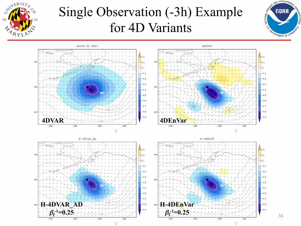
Single Observation (-3h) Example for 4D Variants
36
4DVAR
H-4DVAR_AD βf
-1=0.25 H-4DEnVar βf
-1=0.25
4DEnVar
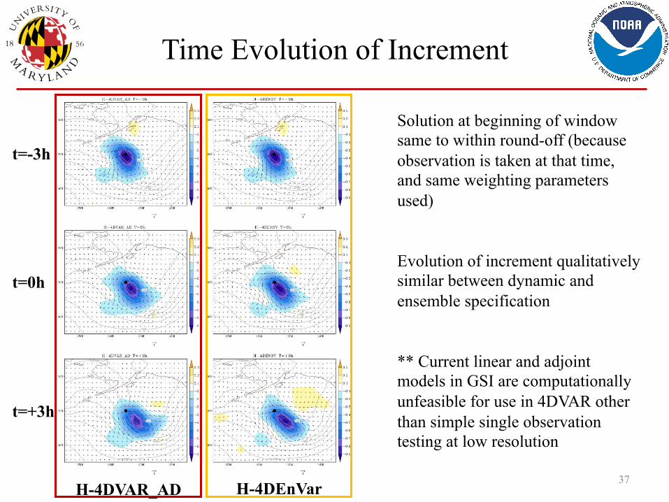
Time Evolution of Increment
37
t=-3h
t=0h
t=+3h
H-4DVAR_AD H-4DEnVar
Solution at beginning of window same to within round-off (because observation is taken at that time, and same weighting parameters used) Evolution of increment qualitatively similar between dynamic and ensemble specification ** Current linear and adjoint models in GSI are computationally unfeasible for use in 4DVAR other than simple single observation testing at low resolution

38
OSSE Cycling Experiments Hybrid 4DEnVar rela>ve to 3DEnVar
Kleist and Ide 2014 (MWR)
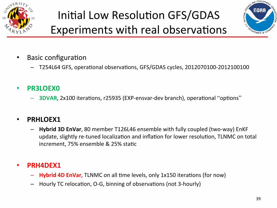
Ini>al Low Resolu>on GFS/GDAS Experiments with real observa>ons
39
• Basic configura>on – T254L64 GFS, opera>onal observa>ons, GFS/GDAS cycles, 2012070100-‐2012100100
• PR3LOEX0 – 3DVAR, 2x100 itera>ons, r25935 (EXP-‐ensvar-‐dev branch), opera>onal “op>ons”
• PRHLOEX1 – Hybrid 3D EnVar, 80 member T126L46 ensemble with fully coupled (two-‐way) EnKF
update, slightly re-‐tuned localiza>on and infla>on for lower resolu>on, TLNMC on total increment, 75% ensemble & 25% sta>c
• PRH4DEX1 – Hybrid 4D EnVar, TLNMC on all >me levels, only 1x150 itera>ons (for now) – Hourly TC reloca>on, O-‐G, binning of observa>ons (not 3-‐hourly)

500 hPa Die Off Curves
40
Northern Hemisphere Southern Hemisphere
4DHYB-3DHYB
3DVAR-3DHYB
Move from 3D Hybrid (current operations) to Hybrid 4D-EnVar yields improvement that is about 75% in amplitude in comparison from going to 3D Hybrid from 3DVAR.
4DHYB ---- 3DHYB ---- 3DVAR ----
4DHYB ---- 3DHYB ---- 3DVAR ----

Extratropical Geop. Height RMSE Differences
41
3DVAR-3DHYB
4DHYB-3DHYB
3DVAR-3DHYB
4DHYB-3DHYB
Northern Hemisphere Southern Hemisphere
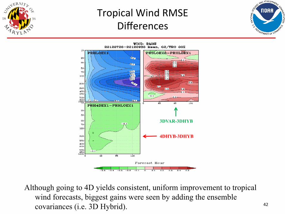
Tropical Wind RMSE Differences
42
3DVAR-3DHYB
4DHYB-3DHYB
Although going to 4D yields consistent, uniform improvement to tropical wind forecasts, biggest gains were seen by adding the ensemble covariances (i.e. 3D Hybrid).

Recent Low Resolu>on GFS/GDAS Experiments with real observa>ons
43
• Due to the impending implementa>on of the new Semi-‐Lagrangian model, tests needed to be redone with new model, configura>on, etc.
• T670 Semi-‐Lagrangian with an 80 member T254 Semi-‐Lagrangian ensemble – Similar ra>o to what is to be implemented with T1543/T574 system – Experiments with both addi>ve infla>on and stochas>c physics as
replacement • Stoch. Physics is resolu>on sensi>ve, requires tuning.
• Compare hybrid 3DEnVar to 4DEnVar (minimal addi>onal tuning such as localiza>on, weights, etc.)

3D v 4D hybrid in SL GFS
44
Northern Hemisphere Southern Hemisphere
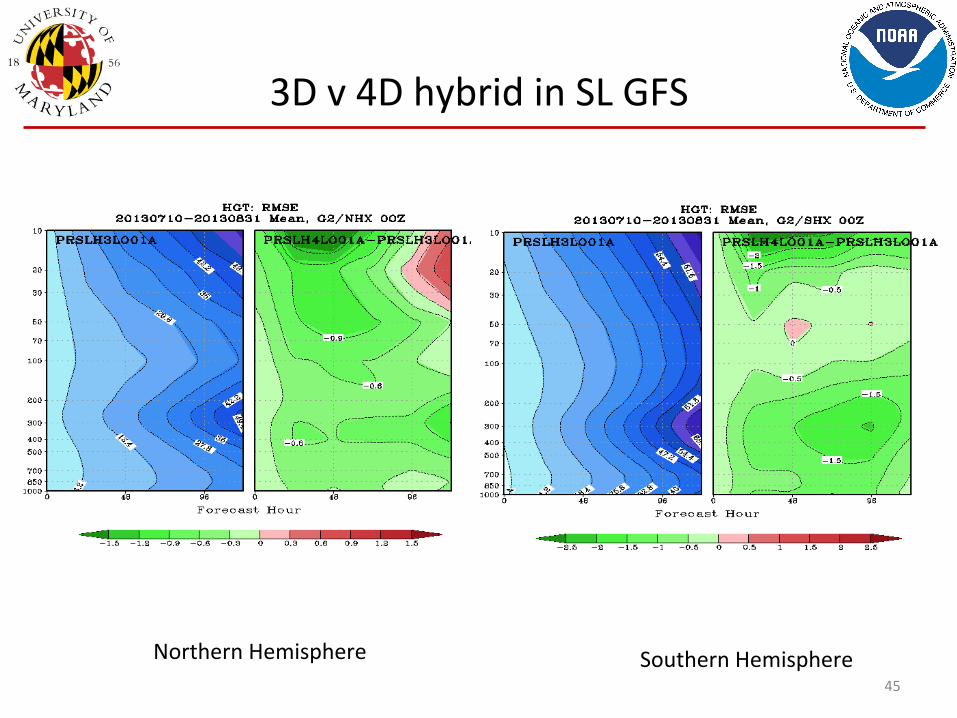
45
3D v 4D hybrid in SL GFS
Northern Hemisphere Southern Hemisphere

Stochas>c Physics Tuning
46
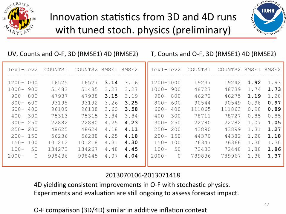
Innova>on sta>s>cs from 3D and 4D runs with tuned stoch. physics (preliminary)
47
lev1-lev2 COUNTS1 COUNTS2 RMSE1 RMSE2 --------------------------------------- 1200-1000 16525 16527 3.14 3.16 1000- 900 51483 51485 3.27 3.27 900- 800 47937 47938 3.15 3.19 800- 600 93195 93192 3.26 3.25 600- 400 96109 96108 3.60 3.58 400- 300 75313 75315 3.84 3.84 300- 250 22882 22880 4.25 4.23 250- 200 48625 48624 4.18 4.11 200- 150 56236 56238 4.25 4.18 150- 100 101212 101218 4.31 4.30 100- 50 134273 134267 4.48 4.45 2000- 0 998436 998445 4.07 4.04
UV, Counts and O-‐F, 3D (RMSE1) 4D (RMSE2)
2013070106-‐2013071418
lev1-lev2 COUNTS1 COUNTS2 RMSE1 RMSE2 --------------------------------------- 1200-1000 19237 19242 1.92 1.93 1000- 900 48727 48739 1.74 1.73 900- 800 46272 46275 1.19 1.20 800- 600 90544 90549 0.98 0.97 600- 400 111865 111863 0.90 0.89 400- 300 78711 78727 0.85 0.85 300- 250 22780 22782 1.07 1.05 250- 200 43890 43899 1.31 1.27 200- 150 44370 44382 1.20 1.18 150- 100 76347 76366 1.30 1.30 100- 50 72433 72448 1.88 1.86 2000- 0 789836 789967 1.38 1.37
T, Counts and O-‐F, 3D (RMSE1) 4D (RMSE2)
4D yielding consistent improvements in O-‐F with stochas>c physics. Experiments and evalua>on are s>ll ongoing to assess forecast impact. O-‐F comparison (3D/4D) similar in addi>ve infla>on context

4D EnVar: Way Forward
• Natural extension to opera>onal EnVar – Uses varia>onal approach in combina>on with already available 4D
ensemble perturba>ons (covariance es>mates) • No need for development of maintenance of TLM and ADJ models
– Makes use of 4D ensemble to perform 4D analysis – Very asrac>ve, modular, usable across a wide variety of applica>ons and
models • Highly scalable
– And can be improved even further – Aligns with technological/compu>ng advances
• Computa>onally inexpensive rela>ve to 4DVAR (with TL/AD) – Es>mates of improved efficiency by 10x or more, e.g. at Env. Canada (6x
faster than 4DVAR on half as many cpus) • Compromises to gain best aspects of (4D) varia>onal and ensemble
DA algorithms • Other centers pursuing similar path forward for determinis>c NWP
– UKMO, Canada (implemented this year)

Implementa>on Plans
• Results are very encouraging, but much work remains – Computa>onal efficiency improvements – Tuning (localiza>on, weigh>ng) – Ini>aliza>on
• Turn off DFI, use TLNMC (default is to currently use over all >me levels), 4DIAU?
– Outer loops – Variable choices for ensemble
• Ini>al implementa>on simply relied on GSI control variables, perhaps not best choice
– Exploring trade space between ensemble size and resolu>on – I/O becoming more and more of an issue, need to address problem head on
• Short term solu>on is likely to u>lize ensemble post-‐processor to precompute ensemble perturba>ons on GSI subdomains
• Target: Late 2015/early 2016 (some of this is machine dependent as NCEP gets their next upgrade) 49
More work to do
• Other poten>al things to add: – Ideas for improving sta>c contribu>on (use slides from Andrew’s Talk? VT guys?
– Ensemble size sensi>vity?
50

51
Single wind observa>on at start of 6 hour window, in jet
0 3 6
Background trajectory
Ob is at l at time 0.
The following slides are from Lorenc et al. 2014
52 © Crown copyright Met Office Andrew Lorenc 52
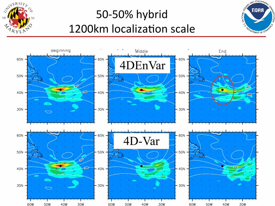
50-‐50% hybrid 1200km localiza>on scale
4DEnVar
4D-Var

Summary from Lorenc et al. 2014 for UKMO system
53
1. The main error in our hybrid-‐4DEnVar (v hybrid-‐-‐4DVar) is that the climatological covariance is used as in 3D-‐Var.
2. 3D localiza>on not following the flow is not an important error for our 1200km localiza>on scale and 6hour window, but does become important for a 500km scale.
3. Proposed solu>ons: Bigger ensemble, beser localiza>on, beser ensemble genera>on (for their system)

Impact of increasing ensemble size in the global EnKF
or How much can we benefit get from increasing ensemble size before model error swamps
sampling error?
Jeff Whitaker

Cov(T,U) 250hPa 2013101500
320 members
80 members
Cov of T at 153E, 35N and U everywhere else at 250hPa
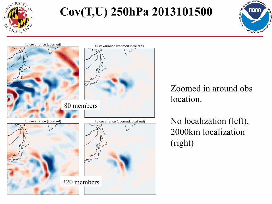
Cov(T,U) 250hPa 2013101500
80 members
320 members
Zoomed in around obs location. No localization (left), 2000km localization (right)
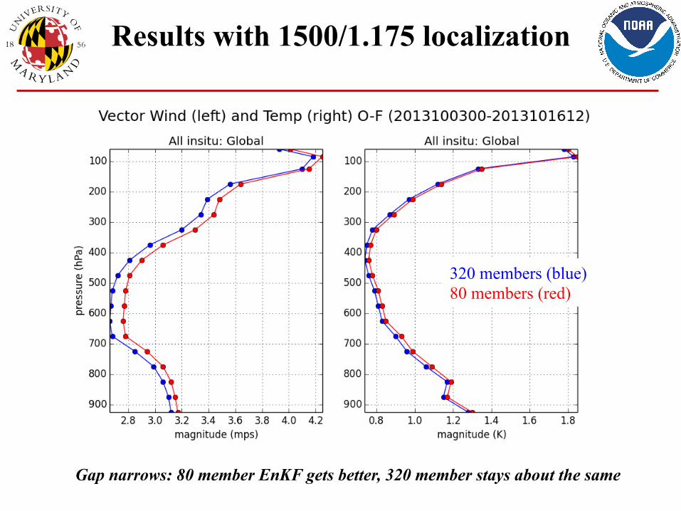
Results with 1500/1.175 localization
Gap narrows: 80 member EnKF gets better, 320 member stays about the same
320 members (blue) 80 members (red)
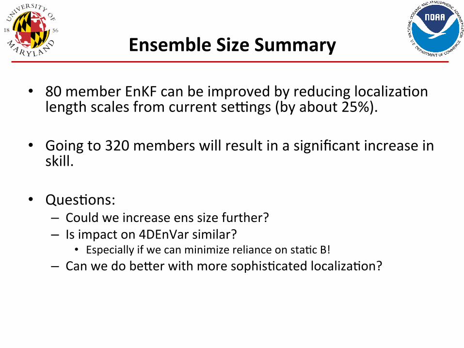
Ensemble Size Summary
• 80 member EnKF can be improved by reducing localiza>on length scales from current sexngs (by about 25%).
• Going to 320 members will result in a significant increase in skill.
• Ques>ons: – Could we increase ens size further? – Is impact on 4DEnVar similar?
• Especially if we can minimize reliance on sta>c B! – Can we do beser with more sophis>cated localiza>on?

Summary
• Significant progress has been made on 4D EnVar development and tes>ng for opera>onal NWP at NCEP
• Further improvements expected through use of improved ini>aliza>on – Removal of DFI, use of 4D IAU – What to do about TLNMC remains open ques>on – Handing of ensemble also important
• Much of the literature shows that hybrid 4DEnVar is not quite as good as hybrid 4DVar – Can close some of this gap with ini>aliza>on (4DIAU) and perhaps
outer loop (to be determined) – Significant work remains in coming up with more op>mal sta>c B
• Finding ways to add temporal component without need for dynamic model in minimiza>on (is it even possible?)
59

• BACKUP
60

TC relocation for EnKF (work done by Yoichiro Ota)
1. Update TC center posi>on (la>tude and longitude) by the EnKF
2. Use updated posi>ons as inputs to the TC reloca>on
3. Apply this procedure before the EnKF analysis and GDAS analysis
Apply TC relocation used in deterministic analysis to each ensemble member, but allowing TC structure perturbations and some TC position spread.
Blue: first guess position Red: Updated position Green: TC vital position
The idea is to separate linear problem (TC location space) and nonlinear problem (actual relocation of fields).

Example: spaghex diagram
Before relocation After relocation
TC relocation of this method can reduce the uncertainty on the TC position, maintaining the TC structure perturbations and some of the position uncertainty. Courtesy Yoichiro Ota
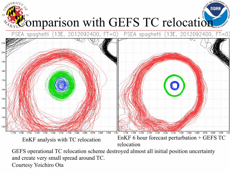
Comparison with GEFS TC relocation
EnKF analysis with TC relocation EnKF 6 hour forecast perturbation + GEFS TC relocation
GEFS operational TC relocation scheme destroyed almost all initial position uncertainty and create very small spread around TC. Courtesy Yoichiro Ota