hw1 solution - professor ting yu's...
TRANSCRIPT

HW1 solution
Problem 1. The answer in not unique.
(1) The probability interpretation of quantum mechanics, which is also called the Copen-
hagen interpretation, is one of the earliest and most commonly taught interpretations of
quantum mechanics. It holds that quantum mechanics does not yield a description of an ob-
jective reality but deals only with probabilities of observing, or measuring, various aspects
of energy quanta, entities that �t neither the classical idea of particles nor the classical
idea of waves. According to the interpretation, the act of measurement causes the set of
probabilities to immediately and randomly assume only one of the possible values. This
feature of the mathematics is known as wavefunction collapse. The essential concepts of
the interpretation were devised by Niels Bohr, Werner Heisenberg and others in the years
1924�27.
Suppose we have a physical observable described by Hermitian operator A, the corre-
sponding eigenvalues are n1, n2, n3, · · · , and the corresponding eigenstates are |n1〉, |n2〉,
|n3〉, · · · . When we perform a measurement on the state
|ψ〉 =∑i
ci|ni〉, (1)
the possible measurement outcomes are just n1, n2, n3, · · · , and the state will collapse into
the corresponding eigenstates |n1〉, |n2〉, |n3〉, · · · . The probability of �nding state |ni〉 is
Pi = |〈ni|ψ〉|2 = |ci|2. (2)
The mean value of the results of the repeated measurements of A is
〈ψ|A|ψ〉 =∑i
Pini. (3)
(2) The relation ∆x∆p > ~2can be regarded as a fundamental limitation on the possibility
of preparing a quantum state |ψ〉 to have statistical dispersions that violate the inequality.
More information about uncertainty relation can be found on Wiki or textbook.
(3) The de Broglie relation shows the concept of matter waves or de Broglie waves and
re�ects the wave�particle duality of matter. It can be expressed as
λ =h
p, (4)
2
where λ is the wavelength of the matter, p is the momentum, and h is the Planck constant.
For the pingpong ball, its wavelength is
λ =h
mv=
6.626Ö10−34m2kg/s
2× 10−3kg × 10m/s= 3.313× 10⁻³²m. (5)
That is why it always di�cult for us to observe quantum e�ect of macroscopic objects,
because their wavelength is so small.
Problem 2.
(a) Measurement results should be the eigenvalues ~2or −~
2. The probabilities are
P+ = |〈+|ψ〉|2 =9
34, (6)
for state |+〉, and
P− = |〈−|ψ〉|2 =25
34, (7)
for state |−〉.
(b) According to the measurement theory of quantum mechanics, the state after mea-
surement collapses into |−〉 immediately. Then, if we perform a subsequent measurement ,
we have 100% probability to obtain |−〉 again.
(c) Performing the measurement to x-component will result in the state �|−〉z� collapse
into the eigenstates of Sx. Since
|−〉z =1√2
(|+〉x − |−〉x), (8)
The probability of �nding |+〉x is
|x〈+|−〉z|2 =1
2(9)
The probability of �nding |−〉x is
|x〈−|−〉z|2 =1
2(10)
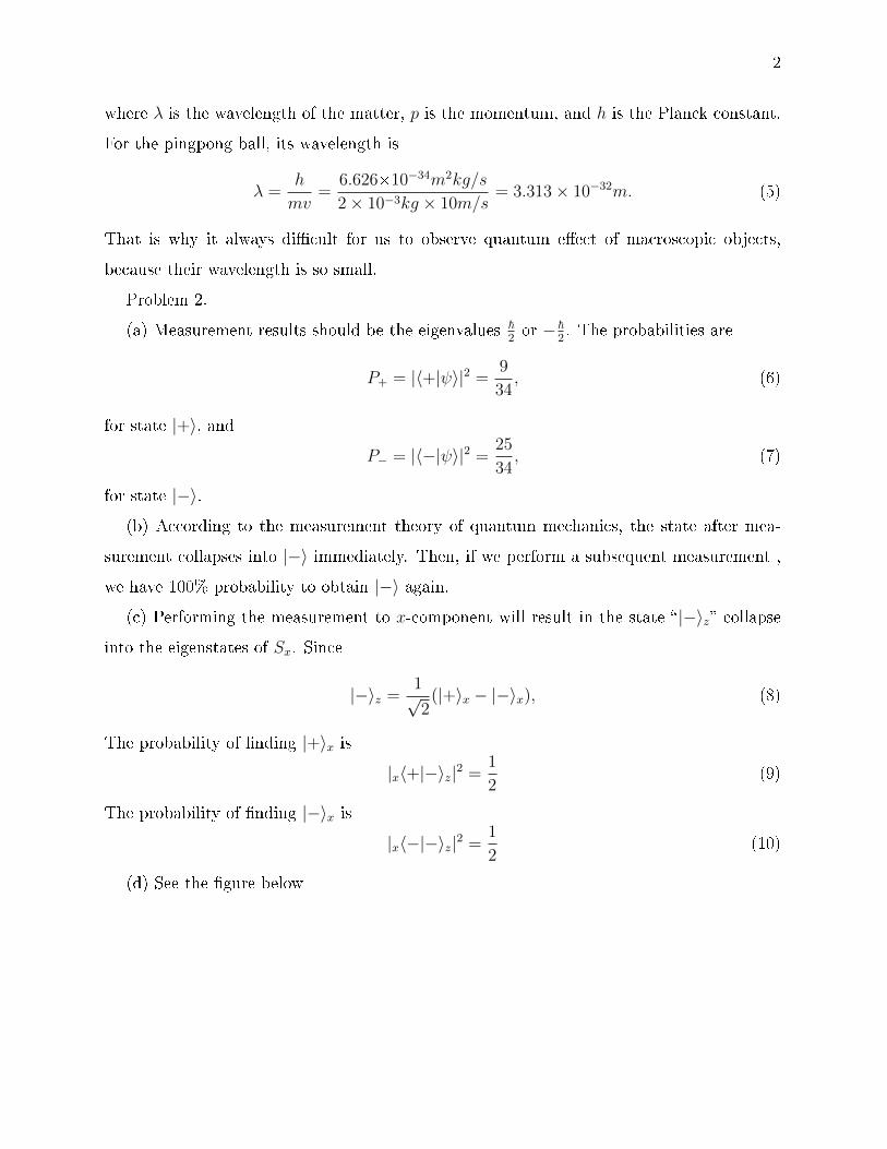
(d) See the �gure below

3
zS
zS
| | z
| z
0% probability to get | z
| z100% probability to get
zS
xS
| | z
| z
50% probability to get | x
| x50% probability to get
Probability: 25/34
Probability: 9/34
Probability: 9/34
Probability: 25/34
Figure 1: diagram of sequential S-G measurements.

HW2 solution
Problem 4.
Write down the Hamiltonian in matrix form in the basis of {|1〉, |2〉} as
H = E
1 1
1 −1
(1)
The solve the Secular equation
det(H − λI) = 0 (2)∣∣∣∣∣∣ E − λ E
E −E − λ
∣∣∣∣∣∣ = 0 (3)
λ2 − E2 − E2 = 0 (4)
λ1 =√2E, λ2 = −
√2E (5)
Then we have
E
1 1
1 −1
ab
=√2E
ab
(6)
So, the eigenstate corresponding to λ1 =√2E is
|ψ1〉 =1√
2 + 2√2[(1 +
√2)|1〉+ |2〉] (7)
Similarly, the eigenstate corresponding to λ2 = −√2E is
|ψ2〉 =1√
2− 2√2[(1−
√2)|1〉+ |2〉] (8)

HW3 solution
1. (a) The coe�cients ak (k = 0, 1, 2, 3) are
2ak = Tr(σkX), (1)
where σ0 = I, σk (k = 1, 2, 3) are Pauli matrices.
Proof:
Tr(IX) = Tr(a0 + a1σ1 + a2σ2 + a3σ3)
= 2a0, (2)
because Tr(σk) = 0 (k = 1, 2, 3).
Tr(σ1X) = Tr[σ1(a0 + a1σ1 + a2σ2 + a3σ3)]
= Tr[a0σ1 + a1 + ia2σ3 − ia3σ2)]
= 2a1. (3)
Similarly,
Tr(σ2X) = 2a2, (4)
Tr(σ3X) = 2a3. (5)
End of proof.
(b) Use the results in (a), we have
a0 =1
2Tr(X)
=1
2Tr
X11 X12
X21 X22
=
1
2(X11 +X22), (6)
a1 =1
2Tr(σ1X)
=1
2Tr
0 1
1 0
X11 X12
X21 X22
=
1
2Tr
X21 X22
X11 X12
=
1
2(X12 +X21), (7)

2
a2 =1
2Tr(σ2X)
=1
2Tr
0 −i
i 0
X11 X12
X21 X22
=
1
2Tr
−iX21 −iX22
iX11 iX12
=
i
2(X12 −X21), (8)
a3 =1
2Tr(σ3X)
=1
2Tr
1 0
0 −1
X11 X12
X21 X22
=
1
2Tr
X11 X12
−X21 −X22
=
1
2(X11 −X22). (9)
2. (a) Choose any complete orthonormal basis {|n〉}, Then TrA =∑
n〈n|A|n〉, therefore,
Tr(XY ) =∑n
〈n|XY |n〉
=∑mn
〈n|X|m〉〈m|Y |n〉
=∑mn
〈m|Y |n〉〈n|X|m〉
=∑m
〈m|Y X|m〉
= Tr(Y X). (10)
(b) From the original de�nition in mathematics, we have two following two mean values
are equal
〈Aψ, φ〉 = 〈ψ,A†φ〉 (11)
where ψ and φ are vectors in Hilbert space, and A can be any operators. According to this,

3
we have
〈(XY )†ψ, φ〉 = 〈ψ, [(XY )†]†φ〉
= 〈ψ,XY φ〉
= 〈X†ψ, Y φ〉
= 〈Y †X†ψ, φ〉. (12)
So,
(XY )† = Y †X†. (13)
(c) Suppose the eigenvalues of A are λn with corresponding eigenvectors |n〉, i.e.,
A|n〉 = λn|n〉. (14)
Then, any function of operator acting on the eigenstate gives
f(A)|n〉 =∑m
f (m)(a)
m!(A− a)m|n〉, (15)
taking the expansion point a = 0, then
f(A)|n〉 =∑m
f (m)(0)
m!Am|n〉
=∑m
f (m)(0)
m!λmn |n〉
= f(λn)|n〉.
Actually, this is the general proof for arbitrary function, exp[if(A)] is just a special case.
Now we compute the matrix elements of it as
exp[if(A)] =∑n
exp[if(A)]|n〉〈n|
=∑n
exp[if(λn)]|n〉〈n|. (16)
3. (1) Since
ψ1 = 〈u1|ψ〉 = c1 (17)
ψ2 = 〈u2|ψ〉 = c2 (18)

4
then,
|ψ〉 =
c1c2
(19)
(2) Calculate every matrix elements as
〈u1|Sz|u1〉 =~2〈u1|u1〉 =
~2
(20)
〈u1|Sz|u2〉 = −~2〈u1|u2〉 = 0 (21)
〈u2|Sz|u1〉 =~2〈u2|u1〉 = 0 (22)
〈u2|Sz|u2〉 = −~2〈u2|u2〉 = −
~2
(23)
So, the matrix form is
Sz =~2
1 0
0 −1
(24)
(3) Since
ψ1 = 〈v1|ψ〉 =1√2c1 −
1√2c2 (25)
ψ2 = 〈v2|ψ〉 =1√2c1 +
1√2c2 (26)
then,
|ψ〉 =
1√2c1 − 1√
2c2
1√2c1 +
1√2c2
(27)
Then, we calculate matrix elements for Sz as
〈v1|Sz|v1〉 =1
2(〈u1| − 〈u2|)Sz(|u1〉 − |u2〉)
=1
2(〈u1| − 〈u2|)
~2(|u1〉+ |u2〉)
= 0 (28)
〈v1|Sz|v2〉 =1
2(〈u1| − 〈u2|)Sz(|u1〉+ |u2〉)
=1
2(〈u1| − 〈u2|)
~2(|u1〉 − |u2〉)
=~2
(29)

5
〈v2|Sz|v1〉 =1
2(〈u1|+ 〈u2|)Sz(|u1〉 − |u2〉)
=1
2(〈u1|+ 〈u2|)
~2(|u1〉+ |u2〉)
=~2
(30)
〈v2|Sz|v2〉 =1
2(〈u1|+ 〈u2|)Sz(|u1〉+ |u2〉)
=1
2(〈u1|+ 〈u2|)
~2(|u1〉 − |u2〉)
= 0 (31)
So, the matrix form in this basis is
Sz =~2
0 1
1 0
(32)
From the relation
|v1〉 =1√2(|u1〉 − |u2〉) (33)
|v2〉 =1√2(|u1〉+ |u2〉) (34)
we can see
|vi〉 =∑j
Uij|uj〉 (35)
where the transformation matrix is
U =
1√2− 1√
2
1√2
1√2
(36)

HW4 solution
I. PART I
1. (1) Let Sz acting on |+〉 and |−〉
Sz|+〉 =~2[|+〉〈+| − |−〉〈−|]|+〉
=~2[|+〉〈+|+〉 − |−〉〈−|+〉]
=~2|+〉 (1)
Sz|+〉 =~2[|+〉〈+| − |−〉〈−|]|−〉
=~2[|+〉〈+|−〉 − |−〉〈−|−〉]
= −~2|−〉 (2)
So, |+〉 is the eigenstate of Sz with corresponding eigenvalue ~2; |−〉 is the eigenstate of Sz
with corresponding eigenvalue −~2.
(2) Compute the matrix elements as
〈+|I|+〉 = 〈+|(|+〉〈+|+ |−〉〈−|)|+〉 = 1 (3)
〈+|I|−〉 = 〈+|(|+〉〈+|+ |−〉〈−|)|−〉 = 0 (4)
〈−|I|+〉 = 〈−|(|+〉〈+|+ |−〉〈−|)|+〉 = 0 (5)
〈−|I|−〉 = 〈−|(|+〉〈+|+ |−〉〈−|)|−〉 = 1 (6)
Therefore the matrix form of I is
I =
1 0
0 1
(7)
Thus, we show explicitly that I is the identity operator.
(3) In matrix form [see (4)],
Sx =~2
0 1
1 0
(8)

2
Solving the Secular equation, we can �nd the eigenvalues and eigenvectors as
λ1 =~2
(9)
with the corresponding eigenvector
|x1〉 =1√2(|+〉+ |−〉) (10)
and
λ2 = −~2
(11)
with the corresponding eigenvector
|x2〉 =1√2(|+〉 − |−〉) (12)
Similarly, in matrix form [see (4)],
Sy =~2
0 −i
i 0
(13)
Solving the Secular equation, we can �nd the eigenvalues and eigenvectors as
λ1 =~2
(14)
with the corresponding eigenvector
|y1〉 =1√2(−i|+〉+ |−〉) (15)
and
λ2 = −~2
(16)
with the corresponding eigenvector
|y2〉 =1√2(i|+〉+ |−〉) (17)
(4) From (1), it is easy to write down
Sz =~2
1 0
0 −1
(18)
Then, compute the matrix elements of Sx as
〈+|Sx|+〉 = 〈+|~2[|+〉〈−|+ |−〉〈+|]|+〉 = 0 (19)

3
〈+|Sx|−〉 = 〈+|~2[|+〉〈−|+ |−〉〈+|]|−〉 = ~
2(20)
〈−|Sx|+〉 = 〈−|~2[|+〉〈−|+ |−〉〈+|]|+〉 = ~
2(21)
〈−|Sx|−〉 = 〈−|~2[|+〉〈−|+ |−〉〈+|]|−〉 = 0 (22)
Therefore the matrix of Sx is
Sx =~2
0 1
1 0
(23)
Nest, compute the matrix elements of Sy as
〈+|Sy|+〉 = 〈+|~2[i|−〉〈+| − i|+〉〈−|]|+〉 = 0 (24)
〈+|Sy|−〉 = 〈+|~2[i|−〉〈+| − i|+〉〈−|]|−〉 = −i~
2(25)
〈−|Sy|+〉 = 〈−|~2[i|−〉〈+| − i|+〉〈−|]|+〉 = i
~2
(26)
〈−|Sy|−〉 = 〈−|~2[i|−〉〈+| − i|+〉〈−|]|−〉 = 0 (27)
Therefore the matrix of Sx is
Sy =~2
0 −i
i 0
(28)
(5) From (3), we know the eigenstates of Sy are
|y1〉 =1√2(−i|+〉+ |−〉) (29)
|y2〉 =1√2(i|+〉+ |−〉) (30)
Then the matrix elements of Sx in this set of basis is
Sx(1, 1) = 〈y1|Sx|y1〉
=1
2(i〈+|+ 〈−|)~
2[|+〉〈−|+ |−〉〈+|](−i|+〉+ |−〉)
= 0 (31)

4
Sx(1, 2) = 〈y1|Sx|y2〉
=1
2(i〈+|+ 〈−|)~
2[|+〉〈−|+ |−〉〈+|](i|+〉+ |−〉)
= i~2
(32)
Sx(2, 1) = 〈y2|Sx|y1〉
=1
2(−i〈+|+ 〈−|)~
2[|+〉〈−|+ |−〉〈+|](−i|+〉+ |−〉)
= −i~2
(33)
Sx(2, 2) = 〈y2|Sx|y2〉
=1
2(−i〈+|+ 〈−|)~
2[|+〉〈−|+ |−〉〈+|](i|+〉+ |−〉)
= 0 (34)
So, the matrix form of Sx is
Sx =~2
0 i
−i 0
(35)
The matrix elements of Sz in this set of basis is
Sz(1, 1) = 〈y1|Sz|y1〉
=1
2(i〈+|+ 〈−|)~
2[|+〉〈+| − |−〉〈−|](−i|+〉+ |−〉)
= 0 (36)
Sz(1, 2) = 〈y1|Sz|y2〉
=1
2(i〈+|+ 〈−|)~
2[|+〉〈+| − |−〉〈−|](i|+〉+ |−〉)
= −~2
(37)
Sz(2, 1) = 〈y2|Sz|y1〉
=1
2(−i〈+|+ 〈−|)~
2[|+〉〈+| − |−〉〈−|](−i|+〉+ |−〉)
= −~2
(38)
Sz(2, 2) = 〈y2|Sz|y2〉
=1
2(−i〈+|+ 〈−|)~
2[|+〉〈+| − |−〉〈−|](i|+〉+ |−〉)
= 0 (39)

5
So, the matrix form of Sz is
Sz =~2
0 −1
−1 0
(40)
(6) From (3), the eigenvalues of Sx are ~2and −~
2. So, the measurement outcome must
be ~2and −~
2.
(7) According to the measurement theory, the probability of obtaining ~2in the measure-
ment on Sxis
P1 = |〈x1|ψ〉|2
= | 1√2(〈+|+ 〈−|)(cosα|+〉+ sinα|−〉)|2
= | 1√2(cosα + sinα)|2
=1
2| cosα + sinα|2
the probability of obtaining −~2in the measurement on Sx is
P2 = |〈x2|ψ〉|2
= | 1√2(〈+| − 〈−|)(cosα|+〉+ sinα|−〉)|2
= | 1√2(cosα− sinα)|2
=1
2| cosα− sinα|2
(8) It is impossible to determine Sx and Sy at the same time, because they are in-
compatible operators (do not commute). This re�ects the uncertainty relation which is a
fundamental relation of quantum mechanics.

6
II. PART II
(1) First, we write down the matrix form of σx ⊗ σx and σx ⊗ σy
σx ⊗ σx =
0 1
1 0
⊗ 0 1
1 0
=
0 0 0 1
0 0 1 0
0 1 0 0
1 0 0 0
(41)
σx ⊗ σy =
0 1
1 0
⊗ 0 −i
i 0
=
0 0 0 −i
0 0 i 0
0 −i 0 0
i 0 0 0
(42)
then, it is clear to check
(σx ⊗ σx)† = σx ⊗ σx (43)
(σy ⊗ σy)† = σy ⊗ σy (44)
which means they are really hermitian matrix.
(2) Solving the Secular equation, we �nd the eigenvalues and eigenvectors are
λ1 = 1 (45)
with the corresponding eigenvector
|ψ1〉 =1√2
1
0
0
1
(46)
λ2 = 1 (47)

7
with the corresponding eigenvector
|ψ2〉 =1√2
0
1
1
0
(48)
λ3 = −1 (49)
with the corresponding eigenvector
|ψ3〉 =1√2
−1
0
0
1
(50)
λ4 = −1 (51)
with the corresponding eigenvector
|ψ4〉 =1√2
0
−1
1
0
(52)
(3) According to the measurement theory, the measurement results are the eigenvalues
λi, i.e., 1 or −1.
(4) Write down the given state in matrix form as
|ψ〉 = 1√2(|+−〉+ | −+〉) = 1√
2
0
1
1
0
(53)
This is just the second eigenstate |ψ2〉. So, the measurement outcome will be 1, and we will
�nd this state with probability 1, and the probability of �nding other states are zero.
We can check this by computing the probabilities of �nding each eigenstates as
P1 = |〈ψ1|ψ〉|2 = 0 (54)

8
P2 = |〈ψ2|ψ〉|2 = 1 (55)
P3 = |〈ψ3|ψ〉|2 = 0 (56)
P4 = |〈ψ3|ψ〉|2 = 0 (57)
This also prove we will �nd the second eigenstate with probability 1.

HW5a solution
1. See Sakurai, page 35-36 Eq. (1.4.53-1.4.63)
2. (a) In classical mechanics,
[x, F (px)] =∂x
∂x
∂F
∂px− ∂x
∂px
∂F
∂x=∂F (px)
∂px. (1)
(b) In quantum mechanics,
[x, exp(ipxa
~)] = [x,
∑n
( ipxa~ )n
n!]
=∑n
[x,( ipxa~ )n
n!]
=∑n
( ia~ )n
n!(in~pn−1)
= −a∑n
( ipxa~ )n
n!
= −a exp(ipxa~
). (2)
(c) Let |ψ〉 = exp( ipxa~ )|x′〉, then
x|ψ〉 = x exp(ipxa
~)|x′〉
= {exp(ipxa~
)|+ [x, exp(ipxa
~)|]}|x′〉.
= (x′ − a)|ψ〉 (3)
So, |ψ〉 is an eigenstate of x, with the corresponding eigenvalue (x′ − a).
3. Since we know
〈x|p′〉 = ψp′(x) =1√2π~
eip′x/~, (4)
which means the state |p′〉 can be expanded in the |x〉 basis as
|p′〉 =�dx
1√2π~
eip′x/~|x〉. (5)
Therefore,
〈p′|x|α〉 =
�dx
1√2π~
e−ip′x/~〈x|x|α〉
=
�dx
1√2π~
e−ip′x/~x〈x|α〉. (6)

2
On the other hand,
i~∂
∂p′〈p′|α〉 = i~
∂
∂p′
�dx
1√2π~
e−ip′x/~〈x|α〉
= i~�dx
1√2π~
∂
∂p′e−ip
′x/~〈x|α〉
= i~�dx
1√2π~
(−ix/~)e−ip′x/~〈x|α〉
=
�dx
1√2π~
e−ip′x/~x〈x|α〉. (7)
Finally, we prove
〈p′|x|α〉 = i~∂
∂p′〈p′|α〉 (8)
Then, we can write down the Hamiltonian in the momentum basis as
H =p2
2m− mω2~2
2
∂2
∂p2, (9)
by taking
x→ i~∂
∂p, p→ p. (10)

HW5b solution
1. Sakruai 2.13 part (a) only
The operators x and p can be expressed as
x =√
~/2mω(a+ a†), p = i√
~mω/2(a† − a) (1)
Then, we have
〈m|x|n〉 = 〈m|√
~/2mω(a+ a†)|n〉
=√
~/2mω(〈m|√n|n− 1〉+ 〈m|
√n+ 1|n+ 1〉)
=√
~/2mω(√nδm,n−1 +
√n+ 1δm,n+1) (2)
〈m|p|n〉 = 〈m|i√~mω/2(a† − a)|n〉
= i√~mω/2(〈m|
√n+ 1|n+ 1〉 − 〈m|
√n|n− 1〉)
=√
~/2mω(√n+ 1δm,n+1 −
√nδm,n−1) (3)
〈m|{x, p}|n〉 = 〈m|(xp+ px)|n〉
=i~2〈m|(aa† − aa+ a†a† − a†a)|n〉
+i~2〈m|(a†a+ a†a† − aa− aa†)|n〉
=i~2〈m|(1− aa+ a†a†)|n〉
+i~2〈m|(a†a† − aa− 1)|n〉
= i~(√
(n+ 1)(n+ 2)δm,n+2 −√n(n− 1)δm,n−2) (4)
〈m|x2|n〉 =~
2mω〈m|(aa+ aa† + a†a+ a†a†)|n〉
=~
2mω[√n(n− 1)δm,n−2 +
√(n+ 1)(n+ 2)δm,n+2 + (2n+ 1)δm,n] (5)
〈m|p2|n〉 = −mω~2〈m|(a†a† − a†a− aa† + aa)|n〉
= − ~2mω
[√n(n− 1)δm,n−2 +
√(n+ 1)(n+ 2)δm,n+2 − (2n+ 1)δm,n] (6)
2. Proof:

2
(a) Using the de�nition
|α〉 = e−|α|2/2
∞∑n=0
αn√n!|n〉 (7)
〈α|α〉 = e−|α|2∞∑m,n
〈m|(α∗)mαn√m!n!
|n〉
= e−|α|2∞∑m,n
(α∗)mαn√m!n!
〈m|n〉
= e−|α|2∞∑m,n
(α∗)mαn√m!n!
δm,n
= e−|α|2
e|α|2
= 1 (8)
So, the coherent state is normalized.
(b) Similar to Problem 1, the operators x and p can be expressed as
x =√
~/2mω(a+ a†), p = i√
~mω/2(a† − a) (9)
Then,
〈α|x|α〉 = 〈α|√
~/2mω(a+ a†)|α〉
=√~/2mω(α + α∗) (10)
〈α|p|α〉 = 〈α|i√
~mω/2(a† − a)|α〉
= i√~mω/2(α∗ − α) (11)
〈α|x2|α〉 =~
2mω〈α|(aa+ aa† + a†a+ a†a†)|α〉
=~
2mω[α2 + 1 + 2|α|2 + (α∗)2] (12)
〈α|p2|α〉 = −mω~2〈α|(a†a† − a†a− aa† + aa)|α〉
= −mω~2
[α2 − 1− 2|α|2 + (α∗)2] (13)
〈α|(∆x)2|α〉 = 〈α|x2|α〉 − 〈α|x|α〉2
=~
2mω[α2 + 1 + 2|α|2 + (α∗)2]− ~
2mω(α + α∗)2
=~
2mω(14)

3
〈α|(∆p)2|α〉 = 〈α|p2|α〉 − 〈α|p|α〉2
= −mω~2
[α2 − 1− 2|α|2 + (α∗)2] +~
2mω(α∗ − α)2
=mω~
2(15)
Finally,
〈α|(∆x)2|α〉〈α|(∆p)2|α〉 =~
2mω
mω~2
=~2
4(16)
So, coherent state gives the minimum uncertainty relation.
(c) Suppose the so-called �N-P� state exist, it must be a linear combination of Fock states
as
|β〉 =∞∑n=0
cn|n〉, (17)
then,
a†|β〉 = a†∞∑n=0
cn|n〉 =∞∑n=0
cn√n+ 1|n+ 1〉. (18)
From this equation, it is easy to see a†|β〉 do not contain |0〉 component, on the other hand,
a†|β〉 = β|β〉, so β|β〉 =∑∞
n=0 cnβ|n〉 also contain no |0〉 component, i.e., c0 = 0.
Next, from the fact |β〉is the eigenstate of a†
a†|β〉 = β|β〉 (19)
we have∞∑n=0
cn√n+ 1|n+ 1〉 =
∞∑n=0
cnβ|n〉 (20)
Therefore, we derive the recursion formula for the coe�cients
cn+1β = cn√n+ 1 (21)
From this equation, it is clearly that if c0 = 0, then all the coe�cients cn are all zero. Finally,
the state |β〉 become a trivial state
|β〉 = 0 (22)
which is not a well-de�ned state (its norm is zero, not 1).

HW6 solution
1. (1) What we need to prove is
i~∂
∂tU(t) = HU(t) (1)
Simply substituting the de�nition of U(t)
U(t) = e−i~Ht (2)
into the Schrödinger equation, we have
i~∂
∂tU(t) = i~
∂
∂t[e−
i~Ht] = i~(− i
~H)e−
i~Ht = HU(t) (3)
which implies U(t) satis�es the Schrödinger equation. (t→ (t− t0))
(2)
(a)
U(t, t0) = e−i~H(t−t0) = e
i~
eB~2mc
σz(t−t0) (4)
Taking the Taylor expansion as
ei~
eB~2mc
σz(t−t0) =∑n
1
n![eB~2mc
(t− t0)]n(σz)n
=∑n
1
n![eB~2mc
(t− t0)]n(
1 0
0 −1
)n
=∑n
1
n![eB~2mc
(t− t0)]n
1n 0
0 (−1)n
)
=
exp[ eB~2mc
(t− t0)] 0
0 exp[− eB~2mc
(t− t0)]
Finally, in the matrix form, it is
U(t) =
exp[ eB~2mc
(t− t0)] 0
0 exp[− eB~2mc
(t− t0)]
(5)

2
(b)
|α, t〉 = U |α〉
=
e i~
eB~2mc
(t−t0) 0
0 e−i~
eB~2mc
(t−t0)
ab
=
ae i~
eB~2mc
(t−t0) 0
0 be−i~
eB~2mc
(t−t0)
(6)
2. (1) What we need to prove is
i~∂
∂tU(t) = H(t)U(t) (7)
Simply substituting the de�nition of U(t)
U(t) = e−i~� tt0H(t′)dt′ (8)
into the Schrödinger equation, we have
i~∂
∂tU(t) = i~
∂
∂t[e−
i~� tt0H(t′)dt′ ] = i~[− i
~H(t)]U(t) = H(t)U(t) (9)
which implies U(t) satis�es the Schrödinger equation. ( ddt
� tt0H(t′)dt′ = H(t− t0))
(2)
(a)
U(t, t0) = e−i~� tt0H(t′)dt′ = e
i~� tt0
eB(t′)~2mc
dt′σz (10)
In the matrix form, it is
U(t) =
e i~� tt0
eB(t′)~2mc
dt′ 0
0 e−i~� tt0
eB(t′)~2mc
dt′
(11)
(b)
|α, t〉 = U |α〉
=
e i~� tt0
eB(t′)~2mc
dt′ 0
0 e−i~� tt0
eB(t′)~2mc
dt′
ab
=
ae i~� tt0
eB(t′)~2mc
dt′ 0
0 be−i~� tt0
eB(t′)~2mc
dt′
(12)

3
3. (a) In the basis {|L〉, |R〉}, the Hamiltonian can be written as
H = ∆
0 1
1 0
(13)
Solve the eigen-equation H|ψ〉 = E|ψ〉, we will derive the eigenvalues and eigenvectors as
(1) E1 = ∆ with the corresponding eigenvector
|ψ1〉 =1√2
1
1
(14)
(2) E2 = −∆ with the corresponding eigenvector
|ψ2〉 =1√2
1
−1
(15)
(b) The time evolution operator is
U(t) = exp(− i~Ht) = exp[− i
~∆(|L〉〈R|+ |R〉〈L|)t] (16)
and
|L〉 =1√2
(|ψ1〉+ |ψ2〉)
|R〉 =1√2
(|ψ1〉 − |ψ2〉)
The initial state is
|ψ(0)〉 = 〈L|α〉|L〉+ 〈R|α〉|R〉 (17)
Applying this operator to the initial state we will �nd the �nal state as
U(t)|ψ(0)〉 = exp[− i~
∆Ht](〈L|α〉|L〉+ 〈R|α〉|R〉)
= exp[− i~
∆Ht]1√2
[〈L|α〉(|ψ1〉+ |ψ2〉) + 〈R|α〉(|ψ1〉 − |ψ2〉)]
=1√2〈L|α〉(e−
i~∆t|ψ1〉+ e
i~∆t|ψ2〉)
+1√2〈R|α〉(e−
i~∆t|ψ1〉 − e
i~∆t|ψ2〉) (18)
where we use
H|ψ1〉 = ∆|ψ1〉 (19)
H|ψ2〉 = −∆|ψ2〉 (20)

4
In the basis {|L〉, |R〉}, the �nal state is just
|α, t〉 = U(t)|ψ(0)〉
= (〈L|α〉 cosωt− i〈R|α〉 sinωt)|L〉
+ (〈R|α〉 cosωt− i〈L|α〉 sinωt)|R〉 (21)
where ω = ∆~ .
(c) If the initial condition is that the particle in the right side, i.e.,
|ψ(0)〉 =
0
1
(22)
Finally, the solution is
|ψ(t)〉 =
sinωt
cosωt
(23)
and the probability is just
〈L|ψ(t)〉 = sin2 ωt (24)
(d) In the Schrödinger picture, the Schrödinger equation can be written as
i~∂
∂t
A(t)
B(t)
= ∆
0 1
1 0
A(t)
B(t)
(25)
The coupled equation is
i~∂
∂tA(t) = ∆B(t) (26)
i~∂
∂tB(t) = ∆A(t) (27)
Solving this equation, we will �nd the solution is
A(t) = A1 cosωt+ A2 sinωt (28)
B(t) = B1 cosωt+B2 sinωt (29)
Using the initial condition that
A(0) = 〈L|α〉 (30)
B(0) = 〈R|α〉 (31)

5
we will �nd the �nal solution is just the same as it is in (b) which is derived by using the
evolution operator.
(e) It is easy to �nd the Hamiltonian is not Hermitian any more, then the evolution will
not be unitary evolution any more by stone theorem. Therefore the probability may not be
preserved. Here, we will not show the result explicit. In fact, it is very easy to check this
conclusion.
4. If t1 < t2, the right hand side (RHS) is
I1 =1
2
� t
0
dt2
� t2
0
dt1H(t2)H(t1). (32)
If t1 > t2, the right hand side is
I2 =1
2
� t
0
dt1
� t1
0
dt2H(t1)H(t2). (33)
Note that the indexes t1 and t2 are dummy integral indexes, interchanging them we will
found I1 = I2. Therefore, RHS is
RHS = I1 + I2 = 2I2 =
� t
0
dt1
� t1
0
dt2H(t1)H(t2) = LHS. (34)
The proof above can be easily understood by looking at the integral regions plotted in Fig.
1.

6
1t
2t1 2t t
2 1( ) ( )H t H t
1 2( ) ( )H t H t
2I
1I
1 2 1 22 2I I I I I
Figure 1: Integral region

HW7 solution
1. (1) Simply substituting
a =
√mω
2~(x+
ip
mω) (1)
a† =
√mω
2~(x− ip
mω) (2)
into
H = ~ω(a†a+1
2) (3)
we obtain
H = ~ω[√
mω
2~(x− ip
mω)
√mω
2~(x+
ip
mω) +
1
2
]=
mω2
2(x2 +
ixp
mω− ipx
mω+
p2
m2ω2) +
1
2~ω
=mω2
2(x2 − ~
mω+
p2
m2ω2) +
1
2~ω
=p2
2m+
1
2mω2x2 (4)
Thus, we prove the two Hamiltonian are identical.
(2) In the Heisenberg picture,
a(t) = eiHt/~ae−iHt/~
= a+it
~[H, a] +
(it)2
2!~2[H, [H, a]] + · · ·
= a+it
~(−~ω)a+
(it)2
2!~2(−~ω)2a+ · · ·
= a exp(−iωt) (5)
a†(t) = eiHt/~a†e−iHt/~
= a† +it
~[H, a†] +
(it)2
2!~2[H, [H, a†]] + · · ·
= a† +it
~(~ω)a† +
(it)2
2!~2(~ω)2a† + · · ·
= a† exp(iωt) (6)

2
(3) The Heisenberg equations are
d
dta(t) =
i
~[H, a]
=i
~[~ω(a†a+
1
2), a]
= −iωa (7)
d
dta†(t) =
i
~[H, a†]
=i
~[~ω(a†a+
1
2), a†]
= iωa† (8)
(4) According to the equations above associated with the boundary conditions
a(0) = a (9)
a†(0) = a† (10)
the solution is
a(t) = a exp(−iωt) (11)
a†(t) = a† exp(iωt) (12)
2. (a) Arbitrary linear combination of |0〉and |1〉can be expressed as
|ψ〉 = α|0〉+ β|1〉 (13)
then, the mean value of x =√
~2mω
(a+ a†) is
〈ψ|x|ψ〉 = (α∗〈0|+ β∗〈1|)√
~2mω
(a+ a†)(α|0〉+ β|1〉)
=
√~
2mω(α∗〈0|+ β∗〈1|)(β|0〉+ α|1〉+
√2β|2〉)
=
√~
2mω(α∗β + β∗α)
when α = β the mean value take the largest value, e.g.,
|ψ〉 =1√2
(|0〉+ |1〉) (14)
give the largest mean value.

3
(b) In the Schrödinger picture, the state will evolve as
d
dt|ψ(t)〉 = − i
~~ω(a†a+
1
2)|ψ(t)〉
= −iω(a†a+1
2)|ψ(t)〉
Using the boundary condition
|ψ(0)〉 =1√2
(|0〉+ |1〉) (15)
and notice the result in (a), the solution is
|ψ(t)〉 =1√2
(e−12iωt|0〉+ e−
32iωt|1〉) (16)
〈ψ(t)|x|ψ(t)〉 =
√~
2mω(1
2e
12iωte−
32iωt +
1
2e−
12iωte
32iωt)
=
√~
2mωcos(ωt) (17)
In the Heisenberg picture,
a(t) = a exp(−iωt) (18)
a†(t) = a† exp(iωt) (19)
The mean value at time t is
〈ψ(0)|x(t)|ψ(0)〉 =1√2
(〈0|+ 〈1|)√
~2mω
[a(t) + a†(t)]1√2
(|0〉+ |1〉)
=1
2
√~
2mω(〈0|+ 〈1|)(e−iωt|0〉+ eiωt|1〉+ eiωt|2〉)
=1
2
√~
2mω(e−iωt + eiωt)
=
√~
2mωcos(ωt) (20)
which is the same as we derived in Schrödinger picture.
(c) We have already compute 〈x〉 in (b), here, we just need to compute 〈x2〉 = ~2mω〈aa+
aa† + a†a+ a†a†〉. In the Schrödinger picture, the state will evolve as
|ψ(t)〉 =1√2
(e−12iωt|0〉+ e−
32iωt|1〉) (21)

4
〈ψ(t)|x2|ψ(t)〉 =~
4mω(e
12iωt〈0|+ e
32iωt〈1|)(aa+ aa† + a†a+ a†a†)(e−
12iωt|0〉+ e−
32iωt|1〉)
=~
4mω(e
12iωt〈0|+ e
32iωt〈1|)(e−
12iωt|0〉+ 3e−
32iωt|1〉+ · · · )
=~
4mω(1 + 3)
=~mω
(22)
Finally,
〈(∆x)2〉 = 〈x2〉 − 〈x〉2
=~mω− ~
2mωcos2(ωt)
=~mω
[1− 1
2cos2(ωt)] (23)
In the Heisenberg picture,
x2(t) =~
2mω[aae−2iωt + aa† + a†a+ a†a†e2iωt] (24)
a(t) = a exp(−iωt) (25)
a†(t) = a† exp(iωt) (26)
The mean value at time t is
〈ψ(0)|x2(t)|ψ(0)〉 =1√2
(〈0|+ 〈1|) ~2mω
[aae−2iωt + aa† + a†a+ a†a†e2iωt]1√2
(|0〉+ |1〉)
=1
2
~2mω
(〈0|+ 〈1|)(|0〉+ 3|1〉+ · · · )
=1
2
~2mω
(1 + 3)
=~mω
(27)
Finally,
〈(∆x)2〉 = 〈x2〉 − 〈x〉2
=~mω− ~
2mωcos2(ωt)
=~mω
[1− 1
2cos2(ωt)] (28)
which is the same as we derived in Schrödinger picture.

5
3. The left hand side is
〈0|eikx|0〉 = 〈0| exp[ik
√~
2mω(a+ a†)]|0〉
= 〈0| exp[ik
√~
2mωa†] exp[ik
√~
2mωa] exp[− ~k2
4mω]|0〉
= exp[− ~k2
4mω] (29)
Then, we compute the right hand side as
exp[−k2〈0|x2|0〉/2] = exp[−k2 ~2mω
/2]
= exp[− ~k2
4mω] (30)
where we use
〈0|x2|0〉 =~
2mω〈0|(aa+ aa† + a†a+ a†a†)|0〉
=~
2mω(31)
Finally, we prove that left hand side and right hand side are equal, i.e.,
〈0|eikx|0〉 = exp[−k2〈0|x2|0〉/2] (32)

HW8a solution
(1) The Heisenberg equation of motion is
d
dtA(t) =
i
~[H,A(t)] (1)
so
d
dta =
i
~[H, a]
=i
~[~ωA
2σz + ~ωa†a+ ~g(σ−a
† + σ+a), a]
= −iωa− igσ− (2)
d
dtσ− =
i
~[H, σ−]
=i
~[~ωA
2σz + ~ωa†a+ ~g(σ−a
† + σ+a), σ−]
= −iωAσ− + igσza
d
dtσz =
i
~[H, σz]
=i
~[~ωA
2σz + ~ωa†a+ ~g(σ−a
† + σ+a), σz]
= 2igσ−a† − 2igσ+a (3)
(2) Proof:
[N,H] = [a†a,~ωA
2σz + ~ωa†a+ ~g(σ−a
† + σ+a)]
+[σ+σ−,~ωA
2σz + ~ωa†a+ ~g(σ−a
† + σ+a)]
= (~gσ−a† − ~gσ+a) + (−~gσ−a† + ~gσ+a)
= 0 (4)

2
[C,H] = [1
2∆σz,
~ωA
2σz + ~ωa†a+ ~g(σ−a
† + σ+a)]
+[gσ+a,~ωA
2σz + ~ωa†a+ ~g(σ−a
† + σ+a)]
+[gσ−a†,~ωA
2σz + ~ωa†a+ ~g(σ−a
† + σ+a)]
= (−∆~gσ−a† + ∆~gσ+a)
+(−g~ωAσ+a+ ~gωσ+a) + ~g2[σ+a, σ−a]
+(g~ωAσ−a† − ~gωσ−a†) + ~g2[σ+a, σ−a]
= 0 (5)
(3) There are two sets of eigen states |e, n〉 |g, n〉, the corresponding eigenvalues are
N |e, n〉 = (a†a+ σ+σ−)|e, n〉 = (n+ 1)|e, n〉 (6)
N |g, n〉 = (a†a+ σ+σ−)|g, n〉 = n|g, n〉 (7)

HW8b solution
(1) Recall Eq. (5.6.17) in the textbook, the zeroth order and �rst perturbations are:
c(0)n (t) = δni (1)
c(1)n (t) =−i~
� t
t0
〈n|Vi(t′)|i〉dt′
=−i~
� t
t0
eiωnit′Vni(t
′)dt′ (2)
then, substituting the potential in this problem V (t) = λ cos(ωt)σx into the zeroth order
and �rst order perturbation, we obtain
c(0)g (t) = 0 (3)
c(0)e (t) = 1 (4)
c(1)e =−i~
� t
t0
eiωeet′Vee(t′)dt′
=−i~
� t
t0
eiωeet′0dt′
= 0 (5)
c(1)g =−i~
� t
t0
eiωget′Vge(t′)dt′
=−i~
� t
t0
eiωget′λ cos(ωt′)dt′
= − iλ2~
� t
0
dt′[ei(ωA+ω)t′ + ei(ωA−ω)t′ ]
= − λ
2~[ei(ωA+ω)t − 1
ωA + ω+ei(ωA−ω)t − 1
ωA − ω] (6)
These are the zeroth order and �rst order approximations.
(2) First, use the relation E − V (x) = 0 to determine the two turning points as
E = V (x) =1
2ω2mx2 (7)
So,
x1 = −√
2E
mω2(8)

2
x2 =
√2E
mω2(9)
Then substituting the result to the integral, we �nd
� x2
x1
dx
√2m(E − 1
2ω2mx2) =
πE
ω(10)
ThereforeπE
ω= ~π(n+
1
2) (11)
Finally,
En = ~ω(n+1
2) (12)
This is the same result as we derived from the exact solution.
(3) Replacing the potential by V = k|x|, and following the same procedure, we obtain
the energy levels in the V -shaped as
En = [3π
4(n+
1
2)]2/3[
e2~2E2
2m]1/3 (13)

HW9 solution
1. Sakurai, problem 3.1
In order to �nd the eigenvalues and eigenvectors of σy, we solve the Secular equation
det(σy − λI) = 0 (1)
Then, it is easy to �nd the eigenvalues are:
λ1 = 1 (2)
with the corresponding eigenvector
|ψ1〉 =1√2
−i1
(3)
and
λ2 = −1 (4)
with the corresponding eigenvector
|ψ2〉 =1√2
i
1
(5)
The probatility of �nding the state |ψ〉 =
α
β
is in the ~/2 state is
|〈ψ1|ψ〉|2 =1
2|iα + β|2 (6)
2. Checking the commutation relation is a quite easy task, we will just give one example

2
here.
[Jx, Jy] =
0 0 0
0 0 −i
0 i 0
0 0 i
0 0 0
−i 0 0
−
0 0 i
0 0 0
−i 0 0
0 0 0
0 0 −i
0 i 0
=
0 0 0
−1 0 0
0 0 0
−0 −1 0
0 0 0
0 0 0
=
0 −1 0
−1 0 0
0 0 0
= iJz (7)
Similarly, we can check all the other commutation relations.
3. The map |α〉 → D(R)|α〉 = |α〉R is surjection, so we can write D(R) as
D(R) =∑n
|αn〉R〈αn| (8)
D(R)†D(R) =∑mn
|αn〉〈αn|RR|αm〉〈αm|
=∑mn
|αn〉δmn〈αm|
= 1 (9)
So, D(R) is unitary.

HW10 solution
1. The Heisenberg equation of motion is
d
dtK1 =
i
~[H,K1]
=i
2~[K2
1
I1+K2
2
I2+K2
3
I3, K1]
=i
2~[i~I2− i~I3]{K2, K3}
=I2 − I32I2I3
{K2, K3} (1)
where we use
[K1, K2] = −i~K3 (2)
[K22 , K1] = K2K2K1 −K1K2K2
= K2(K1K2 + i~K3)− (−K2K1 − i~K3)K2
= i~K2K3 + i~K3K2 (3)
[K23 , K1] = K3K3K1 −K1K3K3
= K3(K1K3 − i~K2)− (K3K1 + i~K2)K3
= −i~K2K3 − i~K3K2 (4)
Similarly, we have
d
dtK2 =
i
~[H,K2] =
I3 − I12I1I3
{K1, K3} (5)
d
dtK3 =
i
~[H,K3] =
I1 − I22I1I2
{K1, K2} (6)
In classical case, K1, K2, K3 commute with each other, then we have e.g.,
d
dtK1 =
I2 − I32I2I3
(K2K3 +K3K2)
=I2 − I32I2I3
2K2K3
=I2 − I3I2I3
I2ω2I3ω3
= (I2 − I3)ω2ω3 (7)

2
Thus, we successfully reproduce Euler's equation.
2. Suppose A commutes with Ji and Jj, then
[A, Jk] = [A,−iεijk[Ji, Jj]]
= −iεijk[A, (JiJj − JjJi)]
= −iεijk{[A, JiJj]− [A, JjJi)]}
= 0 (8)
3. (1) Expand eiθσz as
eiθσz =∑n
1
n!(iθσz)
n
=∑n=odd
1
n!(iθσz)
n +∑
n=even
1
n!(iθσz)
n
=∞∑m=0
(iθ)2m+1
(2m+ 1)!(σz)
2m+1 +∞∑m=0
(iθ)2m
(2m)!(σz)
2m
=∞∑m=0
i(−1)mθ2m+1
(2m+ 1)!σz +
∞∑m=0
(−1)mθ2m
(2m)!I
= iσz sin θ + I cos θ (9)
(2) According to (1),
ei2θσzSxe
− i2θσz = (iσz sin
θ
2+ cos
θ
2)Sx(−iσz sin
θ
2+ cos
θ
2)
= sin2 θ
2σz(
~2σx)σz + i
~2sin
θ
2cos
θ
2[σz, σx] +
~2cos2
θ
2σx
= −~2sin2 θ
2σx +
~2cos2
θ
2σx −
~2σy sin θ
=~2σx cos θ −
~2σy sin θ (10)