human robot cooperation with compliance adaptation along
TRANSCRIPT
Auton RobotDOI 10.1007/s10514-017-9676-3
Human robot cooperation with compliance adaptation alongthe motion trajectory
Bojan Nemec1 · Nejc Likar1 · Andrej Gams1 · Aleš Ude1
Received: 29 December 2016 / Accepted: 17 October 2017© Springer Science+Business Media, LLC 2017
Abstract In this paper we propose a novel approach forintuitive and natural physical human–robot interaction incooperative tasks. Through initial learning by demonstra-tion, robot behavior naturally evolves into a cooperative task,where the human co-worker is allowed to modify both thespatial course of motion as well as the speed of executionat any stage. The main feature of the proposed adapta-tion scheme is that the robot adjusts its stiffness in pathoperational space, defined with a Frenet–Serret frame. Fur-thermore, the required dynamic capabilities of the robotare obtained by decoupling the robot dynamics in oper-ational space, which is attached to the desired trajectory.Speed-scaled dynamic motion primitives are applied for theunderlying task representation. The combination allows ahuman co-worker in a cooperative task to be less precise inparts of the task that require high precision, as the precisionaspect is learned and provided by the robot. The user canalso freely change the speed and/or the trajectory by sim-ply applying force to the robot. The proposed scheme wasexperimentally validated on three illustrative tasks. The first
Electronic supplementary material The online version of thisarticle (https://doi.org/10.1007/s10514-017-9676-3) containssupplementary material, which is available to authorized users.
B Bojan [email protected]
Nejc [email protected]
Andrej [email protected]
Aleš [email protected]
1 Humanoid and Cognitive Robotics Lab, Department ofAutomatics, Biocybernetics and Robotics, Jožef StefanInstitute, Jamova 39, 1000 Ljubljana, Slovenia
task demonstrates novel two-stage learning by demonstra-tion, where the spatial part of the trajectory is demonstratedindependently from the velocity part. The second task showshow parts of the trajectory can be rapidly and significantlychanged in one execution. The final experiment shows twoKuka LWR-4 robots in a bi-manual setting cooperating witha human while carrying an object.
Keywords Human robot coordination · Learning bydemonstration · Dynamic motion primitives · Robotlearning · Robot control
1 Introduction
An important aspect for future use of robots in our homeenvironments as well as in production plants is their abil-ity to cooperate with humans. Robots dominate over humancapabilities in precision and efficiency while performingrepetitive and monotonous tasks, while human are unbeatenin adaptation to new situations and upcoming problems(Faber et al. 2015). Joining both worlds by means of directhuman–robot cooperation brings new advantages and poten-tially solves many open problems in robotics.
Cooperative task execution in physical human–robot inter-action can be classified based on the level of control the robotassumes (Adorno et al. 2011b). Most commonly, the humanand the robot are in master–slave control mode, with theoperator–master–retaining complete control over the evo-lution of the cooperative task. The interaction is providedthrough force or visual feedback (Evrard et al. 2009). Alter-natively, the task can be controlled by the robot and onlyinitiated by the human (Soyama et al. 2004). In some appli-cations, e. g., in rehabilitation robotics (Krebs et al. 1998), thecontrol over the task evolution is dynamically shared betweenthe human and the robot (Mortl et al. 2012). The level of
123
Auton Robot
control can also change based on the current situation. Forexample, when the human is transferring knowledge to therobot, the robot will often be controlled differently than dur-ing the actual execution. The behavior of the robot might alsobe personalized to suit each coworker perfectly. The learningof robot behavior is thus crucial for effective cooperative taskexecution.
However, robotic learning can be applied to variousaspects of the task; for example, the position, the velocity, thelevel of adaptation and/or autonomy, etc. Furthermore, dif-ferent feedback options are available through visual, haptic,or direct physical interaction (Gams 2016). Finally, many ofthese aspects and conditions need to be combined in a single,preferably intuitive, system that allows interaction similar tothat between two humans.
1.1 Problem statement
In this paper we investigate the learning of robot behaviorduringhuman–robot cooperative tasks.Cooperative task con-trol should allow natural learning and adaptive execution.Therefore, it must:
– provide physical human–robot interaction,– allow non-uniform changes of execution speeds,– enable adaptation of a trajectory during its execution,without the need to re-plan the whole task when a newsituation arises,
– provide a certain degree of cooperative intelligence, i. e.,it should be compliant when accuracy is not needed, butstiff when it is needed,
– it should be applicable to both single arm and bimanualhuman–robot cooperation.
pHRI has been heavily investigated in the past (Evrardet al. 2009; Soyama et al. 2004; Krebs et al. 1998; Calinonet al. 2010), including for bimanual robot operations (Adornoet al. 2010; Mortl et al. 2012; Park and Lee 2015). Severalpapers explore sub-aspects of the stated problem. For exam-ple, in a recent paper Ramacciotti et al. (2016) explore sharedcontrol for motion speed and trajectory adaptation. However,to the best of our knowledge, a complete approach that fulfillsthe given problem statement, has not been proposed yet.
In this paper we propose a control architecture, which ful-fills the above problem statement. Throughout execution, therobot constantly learns from the interaction with the human.First, during the initial learning of the task, the control iscompletely handled by the human operator. However, duringthe task repetition, the task is analyzed and the robot gradu-ally takes control over the parts with low variance of executedtrajectories. The human can at any time take back the con-trol over the task execution by again increasing the variancethrough physical interaction.
Initial idea at such a framework was published in Nemecet al. (2016). In this paper we further extend the approachwith (a) passivity based control framework for HRI scheme;(b) improved speed adaptation scheme; (c) additional exper-iments, that prove the validity of the proposed concept.
1.2 Related work
The implementation of a pHRI scheme depends primarilyon the underlaying policy representation, which determinesalso subsequent methods for learning by demonstration, cal-culation of the variability distribution and implementationof non-uniform speed changes. A motor skill necessary toaccomplish the given task does not only comprehend the paththat the robot should follow, but also the variation of coordi-nation patterns during the movement (Calinon et al. 2012).A well known paradigm to cope with such requirements isto encode the task as a dynamical system. Khansari-Zadehand Billard (2011) have introduced a method of encodingmotion as a nonlinear autonomous Dynamical System (DS)and sufficient conditions to ensure global asymptotic stabil-ity at the target. The method uses several demonstrationsand ensures that all motions follow closely the demonstra-tions while ultimately reaching and stopping at the target. Itwas expanded also for fast motions, for example for catchingobjects (Salehian et al. 2016). Themethod relies on Gaussianmixture model (GMM) representation, which was also usedbyCalinon et al. (2014). It sequentially superimposes dynam-ical systems with varying full stiffness matrices. The methodhas been extensively applied, for example also for virtualguides, where the robot is compliant only in the direction ofthe trajectory (Raiola et al. 2015), and for learning of physicalcollaborative human–robot actions (Rozo et al. 2016). Otherapproaches have been proposed for both interactive tasks andfor learning actions from several demonstrations. Mixture ofinteraction primitives has also been proposed (Ewerton et al.2015). An example of learning from several demonstrationsare the probabilistic motion primitives (ProMP) (Paraschoset al. 2013). These enable the encoding of stochastic sys-tem behavior. Modified DMPs to include coupling terms ofdifferent kinds have also been proposed for interaction withhumans in single-arm and bimanual settings (Gams et al.2014). Although these representations allow speed scaling,non-uniform speed scaling in its original form is not possi-ble by either. Recently, interaction tasks have been discussedin a variation of motor primitives called interaction primi-tives (Amor et al. 2014), which maintain a distribution overthe DMP parameters and synchronizes phase with exter-nal agents (e.g. humans) by dynamic time warping. In ourapproach we rely on the framework of dynamicmotion prim-itives (DMP) (Ijspeert et al. 2013) and its extension to copewith non-uniform speed changes (Nemec et al. 2013).
123
Auton Robot
This paper is organized as follows. Section 2 outlines theframework of dynamic movement primitives along with thespeed profile encoding extension. The novelty of the paper isdescribed inSect. 3,which combines the separate sub-aspectsinto a complete algorithm. Applications of the proposedapproach to Learning byDemonstration (LbD) and to biman-ual physical human–robot cooperation are presented in Sect.4. A discussion concludes the paper.
2 Learning by demonstration for human–robotcooperation scheme
In our work we rely on motion representation with dynamicmotion primitives (DMPs) (Ijspeert et al. 2013), extendedfor Cartesian space movements (Ude et al. 2014). Theseare used to encode the demonstrated cooperative human–robot task. Kinesthetic guiding can be used to capture thedesired robot motion. The original DMP formulation doesnot provide the means to variate the speed of movement in anon-uniform way without changing the course of movement.However, in our approach we do need to apply non-uniformspeed changes, prompting the requirement for appropriatetrajectory representation. A suitable representation is Speed-Scaled Dynamic Motion Primitives (SS-DMPs), which weoriginally proposed in (Nemec et al. 2013).
Through kinesthetic guiding we first acquire the initialmovement policy in Cartesian coordinates
G = {pk, qk, pk,ωωωk, pk, ωωωk, tk}Tk=1. (1)
pk ∈ R3 are the positions, while qk ∈ S3 are the unit quater-
nions describing orientation, with S3 denoting a unit spherein R4. Besides the positions and orientations, we also recordthe position and orientation velocities (pk, ωωωk) and accelera-tions (pk, ωωωk). k are trajectory samples, and T is the numberof samples.
We parameterize this demonstrated policy with a nonlin-ear dynamical system that enables the encoding of generaltrajectories (Ijspeert et al. 2013; Nemec et al. 2013; Ude et al.2014). The trajectory can be specified by the following sys-tem of nonlinear differential equations for positions p andorientations q
ν(s)τ z = αz(βz(gp − p) − z + fp(s), (2)
ν(s)τ p = z, (3)
ν(s)τηηη = αz (βz2 log (go ∗ q) − ηηη) + fo(s), (4)
ν(s)τ q = 1
2ηηη ∗ q, (5)
ν(s)τ s = −αss. (6)
Here s denotes the phase and z and ηηη are auxiliary vari-ables. The above system (2)–(6) converges to the unique
equilibrium point at p = gp, z = 0, q = go, ηηη = 0, ands = 0. Asterisk ∗ denotes quaternion multiplication and qquaternion conjugation. Eq. (15) provides the definition ofquaternion logarithm. The nonlinear forcing terms fp(s) andfo(s) are formed in such away that the response of the second-order differential equation system (2)–(6) can approximateany smooth point-to-point trajectory from the initial positionppp0 and orientation qqq0 to the final position gp and orientationgo. The nonlinear forcing terms are defined as linear combi-nations of M radial basis functions (RBFs)
fp(s) =∑M
i=1 wi,p�i (s)∑M
i=1 �i (s)s, (7)
fo(s) =∑M
i=1 wi,o�i (s)∑M
i=1 �i (s)s, (8)
�i (s) = exp(−hi (s − ci )
2)
, (9)
where free parameterswi,p, wi,o determine the shape of posi-tion and orientation trajectories. ci are the centers of RBFs,evenly distributed along the trajectory, with hi their widths.By setting αz = 4βz > 0 and αs > 0, the underlying sec-ond order linear dynamic system (2)–(6) becomes criticallydamped.
Compared to Ude et al. (2014) and analogous to Nemecet al. (2013), we introduced the temporal scaling functionν(s) which is used to specify variations from the demon-strated speed profile. Similarly to the forcing terms (7) and(8), it is encoded as a linear combination of Mv RBFs
ν(s) = 1 +∑Mv
j=1 v j� j (s)∑Mv
j=1 � j (s), (10)
where v j are the corresponding free parameters (weights).In order to parameterize the demonstrated control policy
with a DMP, the weights wi,p, wi,o and v j need to be cal-culated. The shape weights wi,p and wi,o are calculated byapplying standard regression techniques (Ude et al. 2014) andusing the demonstrated trajectory (1) as the target for weightfitting. For ν we initially set v j = 0, i. e. ν = 1, meaningthat the demonstrated speed profile is left unchanged. v j areassigned a different value only through the change of theexecution speed.
2.1 Robot control
Position and orientation trajectories, obtained from DMP,are fed directly to the robot controller as reference values. InpHRI, safety is the primary concern and the robot controllershould exhibit stable operation in all possible interactionswith environments and humans, and should not produceunexpected motions. To achieve this goal we applied the pas-
123
Auton Robot
sivity paradigm for the controller design. It has been widelyused in robotics as it preserves stable operationwith respect tothe feedback and parallel interconnections of passive systems(Hatanaka 2015; Zhang and Cheah 2015). In our study weapplied the two level passivity based impedance controller formanipulators with flexible joints in the form (Albu-Schafferet al. 2007)
ρc = BB−1 u + (I − BB−1
)ρ (11)
u = JT(θθθ)X c + g(θθθ) (12)
whereρc ∈ RN is the control torque input for themotors, N is
number of robot joints,θθθ ∈ RN is the joint positionmeasured
at the motor side, J ∈ RN×6 is the manipulator Jacobian, B
and B ∈ R6×6 denote the positive definite diagonal matrix
of joint and desired joint inertia, respectively. ρ are mea-sured joint torques and g(θθθ) is the gravity vector estimatedin such a way, that it provides exact gravity compensation instatic case using the signals measured at the motor side (Ottet al. 2004). Basically, the role of the motor torque controller(11) is to reduce the motor inertia and to compensate for therobot non-linear dynamics. Desired impedance and dampingis provided with (12).
The task command input X c = [pTc , ωT
c ]T is chosen as
pc = −Dpp + Kpep, (13)
ωc = −Dqω + Kqeq , (14)
where position and orientation tracking errors are definedas ep = pd − p and eq = 2 log(qp ∗ qd). The quaternionlogarithm log : S �→ R
3 is given as
log(q) = log(v, u) =⎧⎨
⎩
arccos(v)u
‖u‖ , u �= 0
[0, 0, 0]T, otherwise. (15)
Its inverse, i. e., the exponential map exp : R3 �→ S, is
defined as
exp(r) =⎧⎨
⎩
cos (‖r‖) + sin (‖r‖) r‖r‖ , r �= 0
1 + [0, 0, 0]T, otherwise. (16)
Subscript (.)d denotes the desired values. Variables without asubscript denote the current values calculated from the robotjoints at themotor side.Kp,Kq ∈ R
3×3 are diagonal, positivedefinite positional stiffness and rotational stiffness matrices,respectively. They specify the properties of the controller inCartesian coordinate system. Positional damping and rota-tional dampingmatricesDp ,Dq ∈ R
3×3 are positive definite,but not necessary diagonal matrices. Proper damping design
is crucial for preserving stability properties of the controller.Unlike in classical computed torque robot controller, damp-ing matrices are configuration dependent. Let’s express totalmanipulator inertia in the task coordinates as
�(θθθ) = (J(θθθ)(H(θθθ) + Bθθθ )−1J(θθθ)T)−1, (17)
where H ∈ RN×N is the manipulator inertia in joint space.
Next, we factorize task inertia as � = �� and proportionalgain matrix as K = KK. K ∈ R
6×6 is composed of Kp andKd . Damping matrix is then calculated as
D = �Dξ K + KDξ �, (18)
where Dξ ∈ R6×6 is a diagonal matrix with the desired
damping. Usually it is set to I for critically damped response.Corresponding Dp and Dq are obtained as upper and lowerpart of the D, respectively. More details about the factor-ization based design of damping matrices can be found in(Albu-Schaffer et al. 2004)
3 Human–robot cooperation scheme
The operation of the proposed system is as follows. First,the human operator demonstrates the desired cooperativehuman–robot motion by kinesthetically guiding the robotarms. The demonstratedmotion is then encoded bySS-DMPsfor position andorientation (p, q) as explained inSect. 2. Thedemonstration of the motion is typically performed slowerthan what is actually the final desired motion, because typ-ically it is not possible to demonstrate the movement withboth high speed and high accuracy. Hence we should allowthe human operator to non-uniformly speed up or slow downthe execution. In our proposed approach this happens on-line during the task execution, when the human co-worker isallowed to modify the motion.
Second, the human operator and the robot iteratively per-form the task several times. The learning of the course ofmotion as well as the learning of the speed profile is basedon the adaptation of the desired trajectory and the estimationof trajectory variances across task repetitions. As suggestedin Calinon et al. (2010), low variance of motion indicatesthat the corresponding part of the task should be executedwith high precision and that no further variations from thecourse of motion should be allowed. If little variance occursin a few executions of the cooperative task, the robot shouldensure precise trajectory tracking by increasing its stiffness inthe directions perpendicular to the direction of motion. Thisallows the human co-worker to decrease his/her own preci-sion as the stiffer robot provides disturbance rejection. Still,the human should be able to speed up the trajectory withoutaffecting the course of motion. To achieve such behavior,
123
Auton Robot
the robot system has to be compliant in the direction ofmotion. To the best of our knowledge, none of the previouslyproposed adaptation algorithms can simultaneously addressthese issues.
3.1 Trajectory adaptation
Initially, in the first iteration of the cooperative task, the robotis uniformly compliant in all directions. Consequently, thecommanded trajectory pl in task repetition cycle l is not thesame as the actually executed trajectory pm due to the inputof the human. Here (.)l is the index of the task repetition,referred to also as learning cycle. Subscript (.)m referrersto the measured coordinates. The proposed adaptation algo-rithm updates the desired trajectory (pl(s), ql(s)), l =1, . . . , L , where the initial SS-DMP is taken from humandemonstration p1, q1, and calculates its variance after eachtask execution.
We update the trajectory and associated covariance matrixusing the following formulas
pl+1(s) = ζ�p(s) + pl(s), (19)
��� p,l+1(s) = (1 − ζ )(��� p,l(s) + ζ�p(s)�p(s)T),
�p(s) = pm(s) − pl(s), (20)
where pm(s) denotes the measured position of the robot,��� p,l(s) is the current cycle covariance of pl(s), all computedat phase x , and ζ ∈ R
[0,1] is the exponentially weightingfactor that defines the learning speed (Knuth 1997). If weset ζ = 1, the updated trajectory pl+1 is equal to the mea-sured trajectory pm . On the other hand, if we set ζ = 0, thetrajectory pl+1 does not change and the system stops learn-ing. After each learning cycle, the updated trajectory pl+1 isencoded into SS-DMP. It is used as the reference trajectory tocontrol the robot in the next cycle.Note that all trajectories arephase dependent, sampled at x(t), t = t1, . . . , tT . The coef-ficients of covariance matrix ��� p,l+1 are approximated witha linear combination of radial basis functions (RBFs). Equa-tion (19) cannot be used for orientation trajectories. Insteadwe apply the following update rule for quaternions
ql+1(s) = exp
(
ζωωω(s)
2
)
∗ ql(s),
ωωω(s) = 2 log(qm(s) ∗ ql(s)). (21)
Similarly, the update rule for variation of orientation trajec-tories can be expressed with
���q,l+1(s) = (1 − ζ )(���q,l(s) + ζωωωl(s)ωωωl(s)T). (22)
3.2 Stiffness adaptation
We dynamically set the desired stiffness of the robot in orderto improve the ease of adaptation. It is well known that theprecision and speed of human motion are related—to be pre-cise, humans reduce their speed (Fitts 1954). While Calinonet al. (2010) proposed to decrease the stiffness in the partsof the trajectory with higher variability and vice versa, wepropose to make the change of stiffness dependent not onlyon the variance but also on the speed of motion. The ideahere is to make the robot compliant when the typically slowfine-tuning of the trajectory is required.
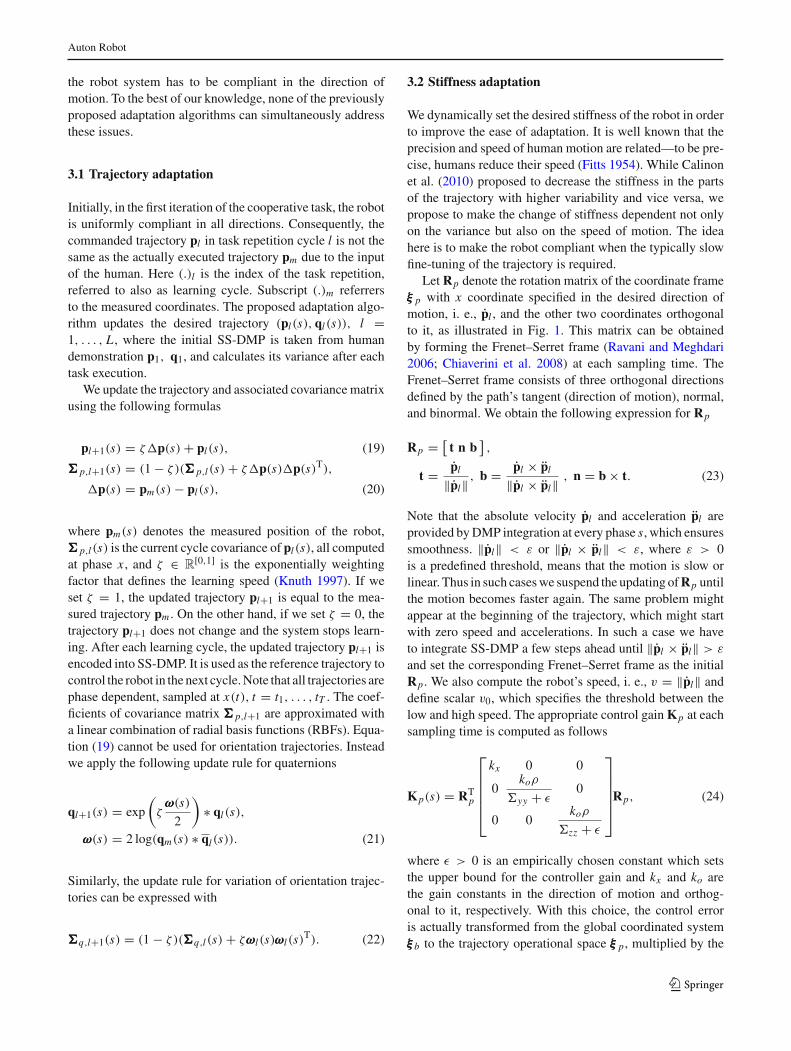
Let Rp denote the rotation matrix of the coordinate frameξξξ p with x coordinate specified in the desired direction ofmotion, i. e., pl , and the other two coordinates orthogonalto it, as illustrated in Fig. 1. This matrix can be obtainedby forming the Frenet–Serret frame (Ravani and Meghdari2006; Chiaverini et al. 2008) at each sampling time. TheFrenet–Serret frame consists of three orthogonal directionsdefined by the path’s tangent (direction of motion), normal,and binormal. We obtain the following expression for Rp
Rp = [t n b
],
t = pl
‖pl‖ , b = pl × pl
‖pl × pl‖ , n = b × t. (23)
Note that the absolute velocity pl and acceleration pl areprovided byDMP integration at every phase s, which ensuressmoothness. ‖pl‖ < ε or ‖pl × pl‖ < ε, where ε > 0is a predefined threshold, means that the motion is slow orlinear. Thus in such caseswe suspend the updating ofRp untilthe motion becomes faster again. The same problem mightappear at the beginning of the trajectory, which might startwith zero speed and accelerations. In such a case we haveto integrate SS-DMP a few steps ahead until ‖pl × pl‖ > ε
and set the corresponding Frenet–Serret frame as the initialRp. We also compute the robot’s speed, i. e., v = ‖pl‖ anddefine scalar v0, which specifies the threshold between thelow and high speed. The appropriate control gain Kp at eachsampling time is computed as follows
Kp(s) = RTp
⎡
⎢⎢⎢⎢⎣
kx 0 0
0koρ
�yy + ε0
0 0koρ
�zz + ε
⎤
⎥⎥⎥⎥⎦
Rp, (24)
where ε > 0 is an empirically chosen constant which setsthe upper bound for the controller gain and kx and ko arethe gain constants in the direction of motion and orthog-onal to it, respectively. With this choice, the control erroris actually transformed from the global coordinated systemξξξb to the trajectory operational space ξξξ p, multiplied by the
123
Auton Robot
)( 4tpξξ
)( 3tpξ
)( 2tpξ
)( 1tpξx
x
x
bξz
x
x y
Fig. 1 Operational space ξξξ p is defined by path orientation
gains defined in the trajectory operational space and rotatedback to the global coordinate system (Khatib 1987).�yy and�zz are the second and the third diagonal coefficient of ���,respectively. Transformation of ��� p,l calculated from errorsmeasured in global coordinate system ξξξb to the trajectorycoordinate system is done by 1985
��� = Rp��� p,l(s)RTp. (25)
Scalarρ scales the control gainswith respect to the calculatedvelocity v. To assure smooth transition of control gains at lowvelocities, it is calculated as
ρ = γ1
(
tanh
(v − v0
γ3
)
− 1
)
+ γ2. (26)
In the above equation, γ1, γ2, γ3 > 0 determine the range,lower bound and the speed of transition between the lowerand upper bound of the switching function defined by tanh,respectively. The initial value for covariance matrix ��� p,1 isset to s0I, where s0 is specified so that we obtain the desiredinitial stiffness orthogonal to the direction of motion. By pre-multiplying and post-multiplying gains with RT
p and Rp, wecan set significantly different stiffnesses in the direction ofmotion and orthogonal to it.
By choosing a constantly low value for kx inKp, the robotis always compliant in the direction of motion, while thestiffness orthogonal to this direction is set according to thelearned variance and speed of motion.
3.3 Speed adaptation
Aspreviously explained, lowgain kx enables the humanoper-ator to freely move the robot in the tangent direction of theFrenet–Serret frame. At the same time, we would like thatthe robot stays on the commanded (learned trajectory) whichmeans, that the human can only anticipate or lag behind thecommanded trajectory. Obviously, this changes the speed of
the trajectory, which is determined by the speed scaling fac-tor ν in Eqs. (2–6). Since all signals which determine thecommanded robot pose are phase dependent, our task is tofind the corresponding phase, which minimizes the differ-ence between the current perturbed robot pose and a pose onthe learned trajectory.
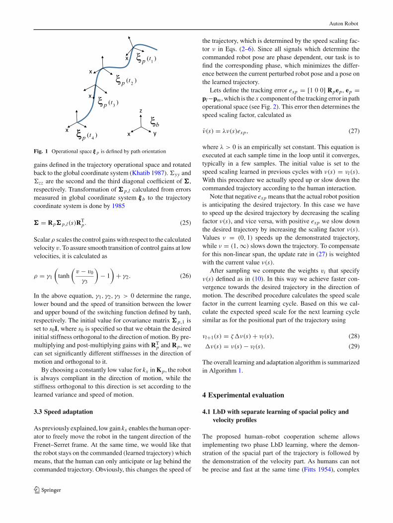
Lets define the tracking error exp = [1 0 0] Rpep, ep =pl−pm , which is the x component of the tracking error in pathoperational space (see Fig. 2). This error then determines thespeed scaling factor, calculated as
ν(s) = λν(s)exp, (27)
where λ > 0 is an empirically set constant. This equation isexecuted at each sample time in the loop until it converges,typically in a few samples. The initial value is set to thespeed scaling learned in previous cycles with ν(s) = νl(s).With this procedure we actually speed up or slow down thecommanded trajectory according to the human interaction.
Note that negative exp means that the actual robot positionis anticipating the desired trajectory. In this case we haveto speed up the desired trajectory by decreasing the scalingfactor ν(s), and vice versa, with positive exp we slow downthe desired trajectory by increasing the scaling factor ν(s).Values ν = (0, 1) speeds up the demonstrated trajectory,while ν = (1,∞) slows down the trajectory. To compensatefor this non-linear span, the update rate in (27) is weightedwith the current value ν(s).
After sampling we compute the weights vi that specifyν(s) defined as in (10). In this way we achieve faster con-vergence towards the desired trajectory in the direction ofmotion. The described procedure calculates the speed scalefactor in the current learning cycle. Based on this we cal-culate the expected speed scale for the next learning cyclesimilar as for the positional part of the trajectory using
νl+1(s) = ζ�ν(s) + νl(s), (28)
�ν(s) = ν(s) − νl(s). (29)
The overall learning and adaptation algorithm is summarizedin Algorithm 1.
4 Experimental evaluation
4.1 LbD with separate learning of spacial policy andvelocity profiles
The proposed human–robot cooperation scheme allowsimplementing two phase LbD learning, where the demon-stration of the spacial part of the trajectory is followed bythe demonstration of the velocity part. As humans can notbe precise and fast at the same time (Fitts 1954), complex
123
Auton Robot
Fig. 2 Position tracking error ep is projected to the tangential axis ofthe Frenet–Serret frame at each sampling instance. Wire frame modelshows the commanded robot pose.Actual robot pose, denotedwith solidmodel, is displaced due to the human operator interaction
trajectories can only be demonstrated at low speeds. Duringthe execution, the learned trajectory needs to be accelerated.In many cases, this acceleration is non-uniform. Some partsmay be executed faster and some parts not, often due to thetechnological requirements, e.g., when applying adhesives,welding, etc. The main idea is to demonstrate a complexpolicy at an arbitrary low speed with an arbitrary velocityprofile. Next, the human demonstrates also the velocity partof the trajectory, while the robot maintains the learned spa-cial trajectory. Learning of the spatial part of the trajectoryis performed as usual, e.g. by capturing the desired policyby kinesthetic guidance as described in Sect. 2 using (2)–(6). In the next step, Frenet–Serret frames are computed at
Algorithm 1: Human–robot cooperation algorithm
1 Record {p(k), q(k), tk}Tk=1 using kinesthetic guiding andcalculate SS-DMP parameters from the demonstrated data(p1, q1)
2 Initialize gains kx , ko and set initial covariance matrices��� p,1 = s0I. Approximate coefficients of��� p,1 with a linearcombination of RBFs.
3 set l = 14 while cooperating do5 set initial phase s = 16 while s ≤ smin do7 integrate SS-DMP to obtain pl (s), ql (s) as well as their
velocities and accelerations8 calculate path rotation Rp(s) using (23) and speed v(s)9 calculate Kp(s) and Dp(s) using (24) and (18),
respectively10 execute control law (12) with pl (s), ql (s) as the desired
trajectory11 sample new trajectories pl+1(s), ql+1(s), covariance
matrices��� p,l+1(s), and calculate speed scaling factorνl+1, all at phase s, using (19) – (21), (27)
12 calculate SS-DMP parameters of pl+1, ql+1, including νl+113 approximate coefficients of��� p,l+1 with linear combinations
of RBFs14 set l = l + 1
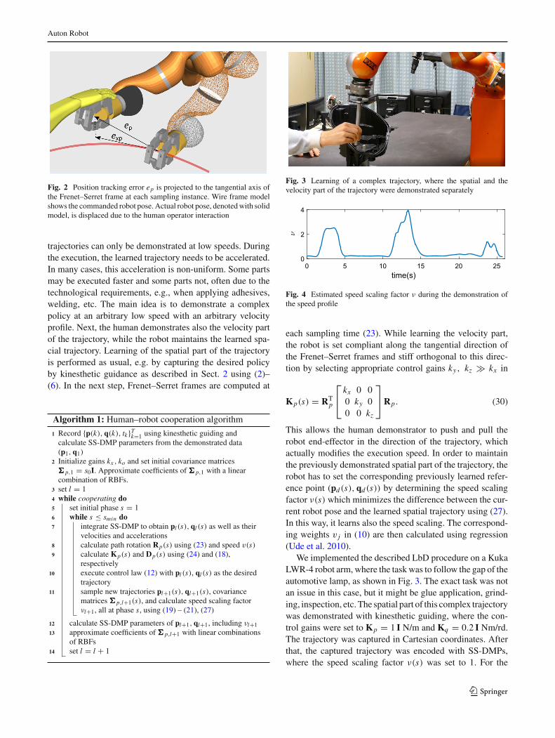
Fig. 3 Learning of a complex trajectory, where the spatial and thevelocity part of the trajectory were demonstrated separately
0 5 10 15 20 25time(s)
0
2
4
νFig. 4 Estimated speed scaling factor ν during the demonstration ofthe speed profile
each sampling time (23). While learning the velocity part,the robot is set compliant along the tangential direction ofthe Frenet–Serret frames and stiff orthogonal to this direc-tion by selecting appropriate control gains ky, kz kx in
Kp(s) = RTp
⎡
⎣kx 0 00 ky 00 0 kz
⎤
⎦ Rp. (30)
This allows the human demonstrator to push and pull therobot end-effector in the direction of the trajectory, whichactually modifies the execution speed. In order to maintainthe previously demonstrated spatial part of the trajectory, therobot has to set the corresponding previously learned refer-ence point (pd(s), qd(s)) by determining the speed scalingfactor ν(s) which minimizes the difference between the cur-rent robot pose and the learned spatial trajectory using (27).In this way, it learns also the speed scaling. The correspond-ing weights v j in (10) are then calculated using regression(Ude et al. 2010).
We implemented the described LbD procedure on a KukaLWR-4 robot arm, where the taskwas to follow the gap of theautomotive lamp, as shown in Fig. 3. The exact task was notan issue in this case, but it might be glue application, grind-ing, inspection, etc. The spatial part of this complex trajectorywas demonstrated with kinesthetic guiding, where the con-trol gains were set to Kp = 1 I N/m and Kq = 0.2 I Nm/rd.The trajectory was captured in Cartesian coordinates. Afterthat, the captured trajectory was encoded with SS-DMPs,where the speed scaling factor ν(s) was set to 1. For the
123

Auton Robot
demonstration of the velocity part of the policy, we raisedthe control gains to kx = 500 N/m, ky, kz = 2000 N/m, andKq = 200 I Nm/rd. During the speed learning, we calcu-late Rp at each sampling time by (23), control gains by (30)and speed scaling by (27). The human operator was able toguide the robot along the previously learned trajectory witharbitrary speed with very low physical effort. For practicalreasons, we limited the learned velocity scale factor to theinterval ν = [0.2, 5]. Figure 4 shows learned speed scaleduring this experiment.
Video of this experiment is available at http://abr.ijs.si/upload/1483017570-TwoPhaseLbD.mp4.
4.2 Coaching with variable stiffness and variableweighting factor
The next experiment demonstrates how to apply the proposedapproach to coaching. The goal of the coaching is to modifyonly a part of the previously learned trajectory while leavingthe rest of the trajectory unchanged (Gams 2016). During thecoaching, it is desirable that we could learn a new part of thetrajectory in single pass while obtaining good disturbancerejection in the part where we would like to preserve thepreviously learned trajectory. To achieve this goal, we applythe compliance adaptation scheme given by the Eqs. (24),(26) and introduce a variable weighting factor ζ in trajectoryupdate (19)–(21). We associate ζ with the tracking error,
ζ(k) =
⎧⎨
⎩
ζmax , ‖ep(k)‖ > d ζmaxζmin
ζmin, ‖ep(k)‖ < dζmind ‖ep(k)‖, otherwise
, (31)
where ζmin and ζmax ∈ R[0,1] are minimal and maximal
exponential weighting factors respectively, and d is theposition error at which point the variable weighting factorstarts to change. In exactly the same way we can associatethe weighting factor to the orientation error. The coachingworks as follows. We drive the robot along the previouslylearned trajectory. Low value of the weighing factor ζmin
and high control gains as a consequence of low values of thecovariance matrices �p and �q provide good disturbancerejection. When we would like to modify the trajectory, wefirst decrease the speed below v0 (26). The system dropsthe stiffness and allows us to modify the trajectory. Con-sequently, the weighting factor changes to ζmax . By settingζmax ≈ 1 the system learns the new trajectory in a singlepass, as it updates it using the current robot configurationsonly.Whenwe re-approach the previously learned trajectory,Eq. (31) decreases ζ . Note that it is required to slow downthe trajectory below v0 only when we want to initiate coach-ing. After that, low compliance will be provided by increasedvalues of the covariance matrices �p and �q . Note also that
Fig. 5 Coaching; the red line is the original trajectory. The blue linedenotes the desired change of the original trajectory (Color figureonline)
it is necessary to calculate the current speed scaling factorν(s) using (27) in each sampling interval in order to get thecorresponding trajectory reference values.
The coachingwas tested for a simple case where the initialtrajectory was learned with a single demonstration. Conse-quently, all of the elements of the covariance matrices �p
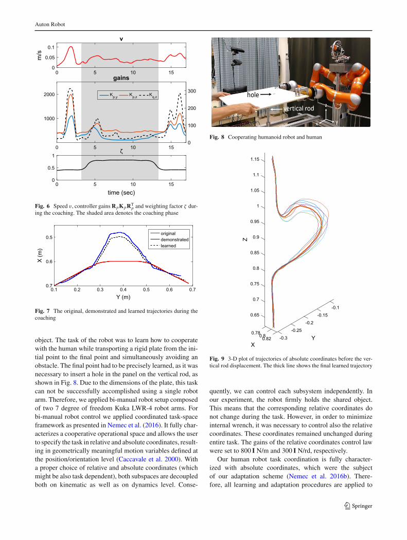
and �q were 0 and the system calculated high control gains.In the next cycle, the operator decreased the speed in orderto decrease the stiffness and demonstrated a new part of thetrajectory. The original and the modified trajectories are pic-tured in Fig. 5 with red and blue lines respectively. In thisexperiment we applied the following settings: ζmin = 0.4,ζmax = 0.8, v0 = 0.07 m/s, d = 0.02 m. In order to makethe coaching even more efficient, the robot reference wasactually the measured position whenever the ζ = ζmax . Thisway, we can apply extensive position and orientation changeswith very little physical effort. Figure 6 shows how the sys-tem adjusted the control gains and weighting factor ζ duringthe coaching. The coaching area is marked with a shadedbackground in the corresponding plots. Note that the gainsare expressed in the trajectory coordinate system, i.e. calcu-lated by (24), before they were pre and post-multiplied withRT
p and Rp, respectively. Resulting robot trajectories are dis-played in Fig. 7. In this plot, the initial trajectory is marked inred. The actual demonstrated trajectory (blue) differs in themiddle part. The learned trajectory is denoted with a blackdotted line. Since ζmax was 0.8, it slightly differs from thedemonstrated one. With ζmax = 1 it would perfectly fol-low the demonstrated trajectory. However, it would be lesssmooth due to the poorer disturbance rejection.
Video of this experiment is available at http://abr.ijs.si/upload/1494512444-Coaching.mp4.
4.3 Bimanual human robot cooperation in objecttransportation
The third experiment involves human robot cooperation(HRC) in transportation of a (potentially large and heavy)
123
Auton Robot
Fig. 6 Speed v, controller gains RpKpRTp and weighting factor ζ dur-
ing the coaching. The shaded area denotes the coaching phase
0.1 0.2 0.3 0.4 0.5 0.6 0.7Y (m)
0.7
0.6
0.5
X (m
)
originaldemonstratedlearned
Fig. 7 The original, demonstrated and learned trajectories during thecoaching
object. The task of the robot was to learn how to cooperatewith the human while transporting a rigid plate from the ini-tial point to the final point and simultaneously avoiding anobstacle. The final point had to be precisely learned, as it wasnecessary to insert a hole in the panel on the vertical rod, asshown in Fig. 8. Due to the dimensions of the plate, this taskcan not be successfully accomplished using a single robotarm. Therefore, we applied bi-manual robot setup composedof two 7 degree of freedom Kuka LWR-4 robot arms. Forbi-manual robot control we applied coordinated task-spaceframework as presented in Nemec et al. (2016). It fully char-acterizes a cooperative operational space and allows the userto specify the task in relative and absolute coordinates, result-ing in geometrically meaningful motion variables defined atthe position/orientation level (Caccavale et al. 2000). Witha proper choice of relative and absolute coordinates (whichmight be also task dependent), both subspaces are decoupledboth on kinematic as well as on dynamics level. Conse-
Fig. 8 Cooperating humanoid robot and human
-0.1
-0.15
Y
-0.2
0.65
-0.25
X
0.780.8
0.7
-0.30.82
0.75
0.8
0.85
0.9Z
0.95
1
1.05
1.1
1.15
Fig. 9 3-D plot of trajectories of absolute coordinates before the ver-tical rod displacement. The thick line shows the final learned trajectory
quently, we can control each subsystem independently. Inour experiment, the robot firmly holds the shared object.This means that the corresponding relative coordinates donot change during the task. However, in order to minimizeinternal wrench, it was necessary to control also the relativecoordinates. These coordinates remained unchanged duringentire task. The gains of the relative coordinates control lawwere set to 800 I N/m and 300 I N/rd, respectively.
Our human robot task coordination is fully character-ized with absolute coordinates, which were the subjectof our adaptation scheme (Nemec et al. 2016b). There-fore, all learning and adaptation procedures are applied to
123
Auton Robot
-0.15
Y
-0.2
-0.25
X
0.65
0.8-0.30.82
0.7
0.75
0.8
0.85
0.9
Z
0.95
1
1.05
1.1
1.15
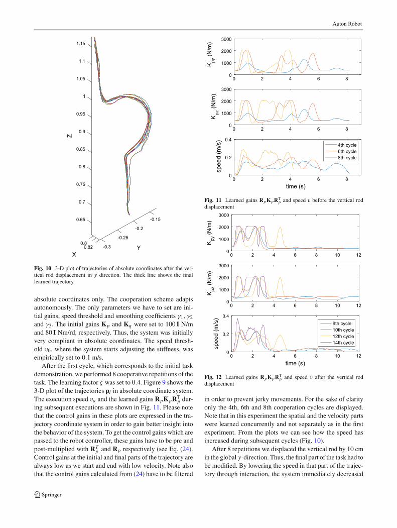
Fig. 10 3-D plot of trajectories of absolute coordinates after the ver-tical rod displacement in y direction. The thick line shows the finallearned trajectory
absolute coordinates only. The cooperation scheme adaptsautonomously. The only parameters we have to set are ini-tial gains, speed threshold and smoothing coefficients γ1, γ2and γ3. The initial gains Kp and Kq were set to 100 I N/mand 80 I Nm/rd, respectively. Thus, the system was initiallyvery compliant in absolute coordinates. The speed thresh-old v0, where the system starts adjusting the stiffness, wasempirically set to 0.1 m/s.
After the first cycle, which corresponds to the initial taskdemonstration, we performed 8 cooperative repetitions of thetask. The learning factor ζ was set to 0.4. Figure 9 shows the3-D plot of the trajectories pl in absolute coordinate system.The execution speed va and the learned gains RpKpRT
p dur-ing subsequent executions are shown in Fig. 11. Please notethat the control gains in these plots are expressed in the tra-jectory coordinate system in order to gain better insight intothe behavior of the system. To get the control gains which arepassed to the robot controller, these gains have to be pre andpost-multiplied with RT
p and Rp respectively (see Eq. (24).Control gains at the initial and final parts of the trajectory arealways low as we start and end with low velocity. Note alsothat the control gains calculated from (24) have to be filtered
0
1000
2000
3000
Kpz
(N/m
)
0
1000
2000
3000
Kpy
(N/m
)
0 2 4 6 8
0 2 4 6 8
0 2 4 6 8time (s)
0
0.2
0.4
spee
d (m
/s)
4th cycle6th cycle8th cycle
Fig. 11 Learned gains RpKpRTp and speed v before the vertical rod
displacement
0
1000
2000
3000
Kpz
(N/m
)
0
1000
2000
3000K
py (N
/m)
8 10 12
8 10 12
0 2 4 6
0 2 4 6
0 2 4 6 8 10 12
time (s)
0
0.2
0.4
spee
d (m
/s)
9th cycle10th cycle12th cycle14th cycle
Fig. 12 Learned gains RpKpRTp and speed v after the vertical rod
displacement
in order to prevent jerky movements. For the sake of clarityonly the 4th, 6th and 8th cooperation cycles are displayed.Note that in this experiment the spatial and the velocity partswere learned concurrently and not separately as in the firstexperiment. From the plots we can see how the speed hasincreased during subsequent cycles (Fig. 10).
After 8 repetitions we displaced the vertical rod by 10 cmin the global y-direction. Thus, the final part of the task had tobe modified. By lowering the speed in that part of the trajec-tory through interaction, the system immediately decreased
123
Auton Robot
the stiffness and allowed for the robot to be guided to the newposition. In order to speed up learning of a new part of thetrajectory, we increased weighting factor ζ to 0.9 in a simi-lar way as in the previous experiment. In a few repetitions,the system learned the new task and re-set the high stiffnessgains. This enabled the human operator to accomplish thetask by allowing the robot to guide him. Also here, for thesake of clarity, we show only the 9th, 10th, 12th and 14thcooperation cycles.
Figure 10 shows the 3-Dplot of trajectoriespl after the dis-placement. Execution speed v and controller gains RpKpRT
pare displayed in Fig. 12.
This experiment is shown also in the video available athttp://abr.ijs.si/upload/1483017628-HRC-Plate.mp4.
5 Conclusions
In this work we proposed a new human–robot cooperationscheme. It can be applied to various tasks, e.g. for (a) twophase LbD with separate demonstration of the spatial andvelocity part of the trajectory, (b) human robot cooperationduring the transportation of heavy and bulky objects, (c) forhuman–robot cooperation during assembly tasks, etc. Thealgorithm can be applied to both single arm as well as bi-manual robotic systems and it doesn’t require force sensing.The developed algorithm is based on the previously proposedSS-DMPs (Nemec et al. 2013) and extended cooperative taskapproach for bi-manual robots (Likar et al. 2015). There areseveral novelties in the proposed approach:
– Speed-scaled DMPs in Cartesian space have been intro-duced.
– Both spatial movement and the speed of cooperativemotion can be adapted.
– Stiffness of the cooperative task is adjusted taking intoaccount the variance of motion across several executionsof the task and the current speed of motion. This enablesthe human to override the learned high stiffness whennecessary.
– Task compliance is defined with respect to the trajectoryoperational space, which allows for varying the dynamicproperties of the system along the direction of motion.
Note that no force sensing is necessary in the proposedapproach, which might decrease the final cost of the setupand increase the robustness, since force measurement is usu-ally noisy. Another advantage of the proposed approach isthe possibility to trim the learning speed and the disturbancerejection with the variable exponential weighting factor ζ .On the other hand, there are many parameters such as thresh-old velocities v0 in (26), weighting factor ζ , initial gains k0and kx in (24), λ in (27) which need careful tuning. In the
future, we will focus on procedures that will either diminishthe number of tuning parameters or learn their values fromprevious experience by means of reinforcement learning.
The proposed schemewas experimentally verified in threeexemplary use-cases. The first is a novel two-phase LbDscheme, which has the potential to be used for learning ofcomplex tasks in industrial setups aswell as for robots appliedin home environments. With the second experiment we showhow to use the proposed scheme in coaching and how to adaptthe weighting factor ζ in order to obtain an appropriate trade-off between the learning speed and disturbance rejection.The third experiment deals with human–robot cooperationin object transportation, which could be applied in assem-bly processes in production plants or in civil engineering fortransportation of heavy and bulky objects.
Acknowledgements The research leading to these results has receivedpartial funding from the Horizon 2020 FoF Research & InnovationAction no. 723909, AUTOWARE, and by the GOSTOP programme,contract no C3330-16-529000, co-financed by Slovenia and the EUunder the ERDF.
References
Adorno, B. V., Bó A. P. L., Fraisse, P., & Poignet, P. (2011). Towardsa cooperative framework for interactive manipulation involving ahuman and a humanoid. In International conference on roboticsand automation (ICRA) (pp. 3777–3783).
Adorno, B., Fraisse, P., &Druon, S. (2010). Dual position control strate-gies using the cooperative dual task-space framework. In IEEE/RSJinternational conference on intelligent robots and systems (IROS),Taipei, Taiwan (pp. 3955–3960).
Albu-Schaffer, A., Ott, C., & Hirzinger, G. (2004). A passivity basedCartesian impedance controller for flexible joint robots—part II:Full state feedback, impedance design and experiments. In IEEEinternational conference on robotics and automation, 2004 pro-ceedings ICRA ’04 2004 3(5) (pp. 2659–2665).
Albu-Schaffer, A., Ott, C., & Hirzinger, G. (2007). A unified passivity-based control framework for position, torque and impedancecontrol of flexible joint robots. The International Journal ofRobotics Research, 26(1), 23–39.
Amor, H. B., Neumann, G., Kamthe, S., Kroemer, O., & Peters, J.(2014). Interaction primitives for human-robot cooperation tasks.In 2014 IEEE international conference on robotics and automation(ICRA) (pp. 2831–2837).
Caccavale, F., Chiacchio, P., & Chiaverini, S. (2000). Task-space regu-lation of cooperative manipulators. Automatica, 36, 879–887.
Calinon, S., Bruno, D., & Caldwell, D. G. (2014). A task-parameterizedprobabilistic model with minimal intervention control. In IEEEinternational conference on robotics and automation (ICRA),Hong Kong (pp. 3339–3344).
Calinon, S., Li, Z., Alizadeh, T., Tsagarakis, N. G., & Caldwell, D.G. (2012). Statistical dynamical systems for skills acquisitionin humanoids. In 12th IEEE-RAS international conference onhumanoid robots (humanoids), Osaka, Japan (pp. 323–329).
Calinon, S., Sardellitti, I., & Caldwell, D. G. (2010). Learning-basedcontrol strategy for safe human-robot interaction exploiting taskand robot redundancies. In IEEE/RSJ international conference onintelligent robots and systems (IROS) (pp. 249–254).
123
Auton Robot
Chiaverini, S., Oriolo, G., & Walker, I. D. (2008). Chapter 11: Kine-matically redundantmanipulators. SpringerHandbook ofRobotics(pp. 245–268). Berlin Heidelberg: Springer.
Evrard, P., Mansard, N., Stasse, O., Kheddar, A., Schauss, T., Weber,C., Peer, A., & Buss, M. (2009). Intercontinental, multimodal,wide-range telecooperation using a humanoid robot. In IEEE/RSJInternational conference on intelligent robots and systems (IROS)(pp. 5635–5640).
Ewerton, M., Neumann, G., Lioutikov, R., Amor, H. B., Peters, J., &Maeda, G. (2015). Learning multiple collaborative tasks with amixture of interaction primitives. In 2015 IEEE International Con-ference on Robotics and Automation (ICRA) (pp. 1535–1542).
Faber, M., Bützler, J., & Schlick, C. M. (2015). Human–robot cooper-ation in future production systems: Analysis of requirements fordesigning an ergonomic work system. ProcediaManufacturing, 3,510–517.
Fitts, P.M. (1954). The information capacity of the humanmotor systemin controlling the amplitude ofmovement. Journal of ExperimentalPsychology, 47(6), 381–391.
Gams, A., Nemec, B., Ijspeert, A. J., &Ude, A. (2014). Couplingmove-ment primitives: Interaction with the environment and bimanualtasks. IEEE Transactions on Robotics, 30(4), 816–830.
Gams, A., Petric, T., Do, M., Nemec, B., Morimoto, J., Asfour, T., et al.(2016). Adaptation and coaching of periodic motion primitivesthrough physical and visual interaction. Robotics and AutonomousSystems, 75(Part B), 340–351.
Hatanaka, T., Chopra, N., & Spong, M.W. (2015). Passivity-based con-trol of robots: Historical perspective and contemporary issues. InConference on decision and control (CDC) (pp. 2450–2452).
Ijspeert, A. J., Nakanishi, J., Hoffmann, H., Pastor, P., & Schaal, S.(2013). Dynamical movement primitives: Learning attractor mod-els for motor behaviors. Neural Computation, 25(2), 328–73.
Khansari-Zadeh, S. M., & Billard, A. (2011). Learning stable nonlineardynamical systems with gaussian mixture models. IEEE Transac-tions on Robotics, 27(5), 943–957.
Khatib, O. (1987). A unified approach for motion and force controlof robot manipulators: The operational space formulation. IEEEJournal of Robotics and Automation, 3, 43–53.
Knuth, D. E. (1997). The Art of computer programming, (3rd ed., Vol.2). Inc, Boston, MA, USA: Seminumerical Algorithms. Addison-Wesley Longman Publishing Co.
Krebs, H. I., Hogan, N., Aisen, M. L., & Volpe, B. T. (1998). Robot-aided neurorehabilitation. IEEE Transactions on RehabilitationEngineering, 6(December), 75–87.
Likar, N., Nemec, B., Zlajpah, L., Ando, S., & Ude, A. (2015).Adaptation of bimanual assembly tasks using iterative learn-ing framework. IEEE-RAS international conference on humanoidrobots (humanoids), Seoul, Korea (pp. 771–776).
Mortl, A., Lawitzky, M., Kucukyilmaz, A., Sezgin, M., Basdogan,C., & Hirche, S. (2012). The role of roles: Physical cooperationbetween humans and robots.The International Journal of RoboticsResearch, 31(13), 1656–1674.
Nemec, B., Gams, A., & Ude, A. (2013). Velocity adaptation for self-improvement of skills learned from user demonstrations. IEEE-RAS International conference on humanoid robots (humanoids),Atlanta, USA (pp. 423–428).
Nemec, B., Likar, N., Gams, A., & Ude, A. (2016a). Adaptive humanrobot cooperation scheme for bimanual robots. In J. Lenarcic & J.Merlet (Eds.), Advances in robot kinematics (pp. 385–393). Roc-quencourt: INRIA.
Nemec, B., Likar, N., Gams, A., & Ude, A. (2016b) Bimanual humanrobot cooperation with adaptive stiffness control. In 16th IEEE-RAS International Conference on Humanoid Robots, Cancun,Mexico (pp. 607–613).
Ott, C., Albu-Schaffer, A., Kugi, A., Stramigioli, S., & Hirzinger, G.(2004). A passivity based cartesian impedance controller for flexi-
ble joint robots-part I: Torque feedback and gravity compensation.In IEEE international conference on robotics & automation (pp.2659–2665).
Paraschos, A., Daniel, C., Peters, J., &Neumann, G. (2013). Probabilis-tic movement primitives. Neural Information Processing Systems,26, 2616–2624.
Park, H. A., & Lee, C. S. G. (2015). Extended cooperative task spacefor manipulation tasks of humanoid robots. In IEEE internationalconference on robotics and automation (ICRA), Seattle, WA (pp.6088–6093).
Raiola, G., Lamy, X., & Stulp, F. (2015). Co-manipulation with mul-tiple probabilistic virtual guides. In 2015 IEEE/RSJ internationalconference on intelligent robots and systems (IROS) (pp. 7–13).
Ramacciotti, M., Milazzo, M., Leoni, F., Roccella, S., & Ste-fanini, C. (2016). A novel shared control algorithm forindustrial robots. International Journal of Advanced RoboticSystems, 13(6), 1729881416682701. https://doi.org/10.1177/1729881416682701.
Ravani, R., & Meghdari, A. (2006). Velocity distribution profile forrobot armmotion using rational Frenet–Serret curves. Informatica,17(1), 69–84.
Rozo, L., Calinon, S., Caldwell, D. G., Jimnez, P., & Torras, C.(2016). Learning physical collaborative robot behaviors fromhuman demonstrations. IEEE Transactions on Robotics, 32(3),513–527.
Salehian, S. S.M., Khoramshahi,M.,&Billard, A. (2016). A dynamicalsystem approach for softly catching a flying object: Theory andexperiment. IEEE Transactions on Robotics, 32(2), 462–471.
Soler, T., & Chin, M. (1985). On transformation of covariance matri-ces between local cartesian coordinate systems and commutativediagrams. In Proceedings of 45th Annual Meeting ACSM-ACSMConvention (pp. 393–406).
Soyama, R., Ishii, S., & Fukase, A. (2004). Selectable operating inter-faces of the meal-assistance device “my spoon”. In Z. Bien & D.Stefanov (Eds.), Rehabilitation (pp. 155–163). Berlin: Springer.
Ude, A., Gams, A., Asfour, T., & Morimoto, J. (2010). Task-specificgeneralization of discrete and periodic dynamic movement primi-tives. IEEE Transactions on Robotics, 26(5), 800–815.
Ude, A., Nemec, B., Petric, T., & Morimoto, J. (2014). Orientation incartesian space dynamicmovement primitives. IEEE internationalconference on robotics and automation (ICRA), HongKong, China(pp. 2997–3004).
Zhang, J., & Cheah, C. C. (2015). Passivity and stability of human–robot interaction control for upper-limb rehabilitation robots. IEEETransactions on Robotics, 31(2), 233–245.
Bojan Nemec received the Di-ploma degree in electrical engi-neering and the M.Sc. and Ph.D.degrees in robotics from the Uni-versity of Ljubljana, Slovenia, in1979, 1982, and 1988. He is cur-rently the Head of the Humanoidand Cognitive Robotics Lab anda SeniorResearchAssociatewiththe Department of Automatics,Biocybernetics, and Robotics,Jožef Stefan Institute, Universityof Ljubljana. He spent his sab-batical leave with the Institutefor Real-Time Computer Sys-
tems and Robotics, University of Karlsruhe, Germany, in 1993. Hisresearch interests include robot control, robot learning, service robotics,and sports biomechanics.
123
Auton Robot
Nejc Likar received the Di-ploma degree in electrical engi-neering in 2009, and the Ph.D.degree in robotics from the JozefStefan International Postgrad-uate school, Ljubljana, Slove-nia, in 2014. He is currentlya Research Fellow with theDepartment of Automatics, Bio-cybernetics, and Robotics, JozefStefan Institute, Ljubljana. Hisresearch interests include bi-manual robot control and huma-noid robot learning.
Andrej Gams received the Di-ploma degree in electrical engi-neering in 2004, and the Ph.D.degree in robotics from the Uni-versity of Ljubljana, Slovenia, in2009. He is currently a ResearchFellow with the Department ofAutomatics, Biocybernetics, andRobotics, Jozef Stefan Institute,Ljubljana. He was a PostdoctoralResearcher with the BioroboticsLaboratory, Ecole PolytechniqueFederale deLausanne, Lausanne,Switzerland, during 2012–2013.His research interests include
imitation learning, control of periodic tasks, and humanoid cognition.
Aleš Ude received the Diplomadegree in applied mathematicsfrom the University of Ljubl-jana, Slovenia, in 1990 and aDr.-Eng. sciences degree fromthe Faculty of Informatics, Uni-versity of Karlsruhe, Karlsruhe,Germany, in 1995. He is head ofthe Department of Automatics,Biocybernetics, and Robotics,Jožef Stefan Institute, Ljubl-jana. He is also associated withthe ATR Computational Neu-roscience Laboratories, Kyoto,Japan. His research interests
include autonomous robot learning, imitation learning, humanoidrobot vision, perception of human activity, humanoid cognition, andhumanoid robotics in general.
123