저 시-비 리- 경 지 2.0 한민

는 아래 조건 르는 경 에 한하여 게

l 저 물 복제, 포, 전송, 전시, 공연 송할 수 습니다.

다 과 같 조건 라야 합니다:

l 하는, 저 물 나 포 경 , 저 물에 적 된 허락조건 명확하게 나타내어야 합니다.

l 저 터 허가를 면 러한 조건들 적 되지 않습니다.

저 에 른 리는 내 에 하여 향 지 않습니다.

것 허락규약(Legal Code) 해하 쉽게 약한 것 니다.

Disclaimer

저 시. 하는 원저 를 시하여야 합니다.

비 리. 하는 저 물 리 목적 할 수 없습니다.

경 지. 하는 저 물 개 , 형 또는 가공할 수 없습니다.

Master's Thesis

Kinematic Analysis and Path Planning Algorithms of

a Quadruped Robot with Redundant DOFs for

Adaptation on Complex Environment

Hyunkyoo Park

Department of Mechanical Engineering

Graduate School of UNIST

2018

Kinematic Analysis and Path Planning Algorithms of

a Quadruped Robot with Redundant DOFs for

Adaptation on Complex Environment

Hyunkyoo Park

Department of Mechanical Engineering

Graduate School of UNIST

Kinematic Analysis and Path Planning Algorithms of

a Quadruped Robot with Redundant DOFs for

Adaptation on Complex Environment

A thesis/dissertation

submitted to the Graduate School of UNIST

in partial fulfillment of the

requirements for the degree of

Master of Science

Hyunkyoo Park

18. 01. 08

Approved by

_________________________

Advisor

Joonbum Bae

Kinematic Analysis and Path Planning Algorithms of

a Quadruped Robot with Redundant DOFs for

Adaptation on Complex Environment

Hyunkyoo Park

This certifies that the thesis/dissertation of Hyunkyoo Park is approved.

01. 08. 2018

signature

___________________________

Advisor: Joonbum Bae

signature

___________________________

Hungsun Son

signature

___________________________

Sang Hoon Kang

Abstract

This thesis presents a kinematic analysis and path planning algorithms for a quadruped robot with

redundant degrees of freedom (DOFs). The kinematically redundant leg can exploit its redundancy for

various types of locomotion and manipulation. Unlike previously developed quadruped robots, the

proposed robot can suitably adapt to different environments by changing its body posture. For example,

the robot can walk on a plain terrain, pass through a narrow gap, overcome an obstacle, perform a simple

task by using one of its legs as a manipulator, etc. The proposed robot has 7 DOFs in each leg and its

inverse kinematics was analyzed by a newly proposed method: a modified Improved Jacobian

Pseudoinverse (mIJP) algorithm. Previously, an Improved Jacobian Pseudoinverse (IJP) algorithm was

proposed to reduce sharp error at the early stage of the trajectory when the initial posture of the

manipulator is closed to the singularity. However, the IJP algorithm has a necessary condition that the

calculated final position of the end-effector to be converged to the desired position. The mIJP algorithm

is proposed to control the manipulator without such requirement.

Also, a center of gravity (COG) trajectory planning method for the proposed quadruped robot is

proposed in this thesis. The robot has significant COG movement during leg swing phase due to its

heavy weight leg, which is not desired because it may cause instability. Thus, we proposed a new COG

trajectory planning algorithm for stable and efficient walking even though the undesired COG

movement was occurred. By using a combined Jacobian of COG and centroid of a support polygon (SP)

with constraints of foot contact points, all calculations could be conducted in the local frame, and

improved performance for tracking the desired trajectory of COG was attained. Performance of the

proposed method was verified in both simulations and experiments.

Contents

I. Introduction ---------------------------------------------------------------------------------------------1

II. System Analysis ----------------------------------------------------------------------------------------5

1. System Configuration ----------------------------------------------------------------------------5

2. Single-leg Kinematic Analysis ------------------------------------------------------------------7

3. Foot Design ---------------------------------------------------------------------------------------11

III. Modified Improved Jacobian Pseudoinverse (mIJP) Algorithm ---------------------------------13

1. Weighted Least Norm (WLN) method --------------------------------------------------------13

2. Improved Jacobian Pseudoinverse (IJP) Algorithm -----------------------------------------14

3. Modified Improved Jacobian Pseudoinverse (mIJP) Algorithm ---------------------------17

IV. A COG Trajectory Planning Method ----------------------------------------------------------------19

1. Walking Mechanism -----------------------------------------------------------------------------19

2. Stability Criteria ---------------------------------------------------------------------------------22

3. Gait Sequence ------------------------------------------------------------------------------------23

4. A COG Trajectory Planning Method ----------------------------------------------------------25

V. Performance verification by Simulations and Experiments -------------------------------------34

1. Simulation Results -------------------------------------------------------------------------------34

2. Experimental Results ----------------------------------------------------------------------------38

VI. Conclusion and Open Issues -------------------------------------------------------------------------42

List of Figures

Fig. I.1 Previously developed octopus inspired robot

Fig. I.2 The proposed quadruped robots which have 6 joints and 7 joints in each leg

Fig. I.3 Previously developed quadruped robot.

Fig. II.1 The proposed advanced quadruped robot

Fig. II.2 Attached reference frames on the robot

Fig. II.3 Representation of Euler angles ZYZ

Fig. II.4 Considered foot design

Fig. III.1 Joint values during trajectory following

Fig. III.2 Simulation results of the inverse kinematics of the robot’s leg with IJP algorithm

Fig. III.3 Simulation results of the inverse kinematics of the robot’s leg with mIJP algorithm

Fig. IV.1 Static walking

Fig. IV.2 Dynamic walking

Fig. IV.3 Cart-table model of a quadruped robot

Fig. IV.4 Stance posture of the quadruped robot

Fig. IV.5 Definition of longitudinal stability margin

Fig. IV.6 A quadruped robot static walking gait sequences start with leg 1

Fig. IV.7 Double support polygon for two left legs

Fig. IV.8 The undesired COG movement during two right legs swing sequentially

Fig. IV. 9 The COG shift methods.

Fig. IV.10 The proposed position difference vector between the COG and centroid

Fig. IV.11 The position vectors of each leg

Fig. IV.12 Simulation results to coincide the COG to the figure 8 trajectory

Fig. IV.13 The flowchart of the proposed COG trajectory planning algorithm

Fig. IV.14 COG shift plan before two right-side legs swing

Fig. V.1 Snapshots of walking on the plain terrain of the robot during the simulation

Fig. V.2 Simulation results when the robot was commanded to walk on the plain terrain

Fig. V.3 Snapshots of avoiding an obstacle by changing height of the robot during the simulation

Fig. V.4 Snapshots of using one leg as a manipulator of the robot during the simulation

Fig. V.5 Snapshots of passing through a narrow gap of the robot during the simulation

Fig. V.6 Snapshots of walking on the plain terrain of the robot during the experiment

Fig. V.7 Snapshots of avoiding and obstacle by changing height of the robot during the experiment

Fig. V.8 Snapshots of using one leg as a manipulator of the robot during the experiment

Fig. V.9 Snapshots of passing through a narrow gap of the robot during the experiment

List of Tables

Table II.1 Types of manipulator

Table II.2 The specification of the proposed robot

Table II.3 DH table of the single leg

1

I. Introduction

An octopus has eight versatile and compliant legs that can serve as multi-functional purposes such as

grasping, crawling, catching a prey, etc. As shown in Fig. I.1-(a) and (b), several robotic systems have

been developed to mimic the mobility of an octopus by mostly utilizing soft material in underwater [1-

2]. However, those soft robots are lack of versatile mobility on the ground, and thus alternative approach

needs to be investigated.

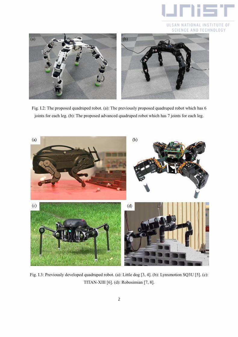
In this thesis, previously, a quadruped robot that has 6 joints in each leg (24 DOFs in total) which only

consider the position of the end-effector was proposed to achieve high degree of functionality and

adaptation in various environments as in Fig. I.2-(a). However, the orientation of the end-effector was

critical for maintaining the stable posture of the robot because the robot easily tumbled due to

inadequate end-effector's orientation. Therefore, we propose an advanced quadruped robot that has 7

joints for each leg as shown in Fig. I.2-(b).

Compared with the similar size of quadruped robot like in Fig. I.3-(a) to (c), our robot was developed

for high-degree of functionality and adaptation in various environments. For example, our robot can

walk on a plain terrain, cross over an obstacle, and pass through a narrow gap by changing its body

posture. Also, the robot can perform a simple task, such as clearing a path, by using one of its leg as a

manipulator. Another similar robot named RoboSimian in Fig. I.3-(c) and (d) has highly dexterous four

7 DOFs limbs for both locomotion and manipulation [7, 8]. To control such high DOFs limbs, an inverse

kinematics look-up table together with a gradient based algorithm was used. However, the proposed

robot is mainly relied on the differential kinematics for the fast calculation time.

Fig. I.1: Previously developed octopus inspired robot [1-2].

2

Fig. I.2: The proposed quadruped robot. (a): The previously proposed quadruped robot which has 6

joints for each leg. (b): The proposed advanced quadruped robot which has 7 joints for each leg.

Fig. I.3: Previously developed quadruped robot. (a): Little dog [3, 4]. (b): Lynxmotion SQ3U [5]. (c):

TITAN-XIII [6]. (d): Robosimian [7, 8].

3

A manipulator which has more degrees of freedom (DOFs) than required for a given task as the

proposed robot leg is called a redundant manipulator. For example, when we consider the position and

orientation both in 3D space, manipulators which have more than 6 DOFs are called redundant

manipulator. A redundant manipulator is typically exploited to perform multiple tasks such as avoiding

the joint limit, obstacles in the workspace, singularities, etc [9].

Many algorithmic approaches have been proposed to control a redundant manipulator. In [10], the

weighted least-norm (WLN) solution was proposed to ensure joint limit avoidance by avoiding

unnecessary self-motions and oscillation. Solving inverse kinematic problems for redundant

manipulators under the two constraints (avoidance of obstacle and joint limits) was introduced in [11]

using the extended Jacobian matrix. Also, a general scheme to manage multiple tasks using a task

priority strategy for redundant robots was studied in [12]. Widely used closed-loop inverse kinematics

methods are well summarized in [13] including damping and filtering of singular values with two

enhancements. A rather different approach was studied in [14] using a modified Newton-Raphson

method with a step size control technique. A method of joint velocity/acceleration redistribution for a

redundant manipulator was introduced in [15] to preserve the joint velocity/acceleration within their

limits. A similar, but, computationally more efficient approach called Saturation in the Null Space (SNS)

iterative algorithm was proposed in [16]. However, near the kinematic singularity posture, they could

not follow the desired trajectory with high accuracy.

Here, we propose a modified Improved Jacobian Pseudoinverse (mIJP) algorithm which mainly relied

on a differential kinematics to control the robot. Improved Jacobian Pseudoinverse (IJP) algorithm was

introduced to prevent sharp error when the initial posture of manipulator is close to kinematic singularity

in [17]. The basic concept of the IJP algorithm was calculating again the given trajectory in reverse

order. For reverse calculation, the IJP algorithm requires the calculated final position of manipulator's

end-effector to be converged to the desired position. However, with the decrease of redundancy by

considering the orientation of the end-effector, it becomes difficult to satisfy this requirement for the

singular posture. Therefore, we modify the IJP algorithm to control manipulator without such

requirement.

Also, we consider an efficient center of gravity (COG) trajectory planning method as it is the primary

concern for stable walking of a quadruped robot. In [18], two sway motions were introduced named Y-

Sway and E-Sway which have different methods to calculate the transversal components of the COG.

In [19], a sinusoidal sway both in moving direction and the transversal direction of the COG was

introduced. In [20], a composite COG trajectory planning method was introduced, which composed of

quintic curves and straight lines. Inverse kinematics using whole-body Jacobian with hybrid approach

4

was introduced in [21], and floating base approach was studied in [22, 23]. In [24], body movement

with the consideration of the body workspace was studied. A zero-moment point (ZMP) [25] based

stability criteria were also considered to maintain a dynamic stability [26, 27]. Even though these works

show great performance to sustain stability of a quadruped robot, they can only be applied when the

robot has global coordinate system or negligible leg weight comparing to the body weight.

Our proposed robot has kinematically redundant legs to exploit its redundancy to perform various

tasks, thus it has heavy weight comparing to the body weight (legs weight/robot weight ≈ 0.8). As a

result, when the robot swings its leg forward, corresponding COG movement is significant. However,

such COG movement is not desired because the COG movement may cross its stability boundary

formed inside the support polygon (SP). Thus, in this thesis, by adding the constraint of the foot contact

points in the combined Jacobian of the COG and centroid of the SP, we proposed a new COG trajectory

planning method for improved stable and efficient walking even though undesired COG movement was

occurred.

The remainder of this thesis is organized as follows. After discussing the system analysis and mIJP

algorithm in Section II and III, we propose the new COG trajectory planning method in Section IV.

Performance is verified by simulations and experiments in Section V. Conclusion and open issues are

summarized in Section VI.

5

II. System Analysis

II.1 System Configuration

As an actuator for a mobile robot, a cable-driven manipulator was studied in [28, 29]. Even though the

cable-driven manipulator can make continuous motion with light weight, its motion is uni-directional

motion which causes the increase of system complexity to make bi-directional motion. In [30, 31],

manipulators using soft actuator was studied. A soft robot arm can make infinite DOFs, thus the

traditional mathematical tools are difficult to apply. Also, it cannot generate high force to overcome the

weight of the robot. Even though the manipulator using a pneumatic actuator can generate relatively

high force, it is hard to precisely control and requires compressed fluid [32]. Therefore, we designed

direct-driven manipulator which consists of a series of short links connected to one another with the use

of discrete joints. The detailed description of the manipulator for each type are introduced in Table II.1.

Type Advantage Disadvantage Example

Cable-driven

manipulator

[28]

▣ Continuous motion

▣ Light body

▣ Unpredictable motion

▣ Uni-directional motion

Soft

manipulator

[30]

▣ Continuous motion

▣ Light body

▣ Unpredictable motion

▣ Generate low force

Pneumatic

manipulator

[32]

▣ Generate relatively

high force

▣ Light body

▣ Hard to control precisely

▣ Require compressed fluid

Direct-driven

manipulator

[33]

▣ Predictable motion

▣ Generate high force

▣ Discrete motion

▣ Heavy body

Table II.1 Types of manipulator

6

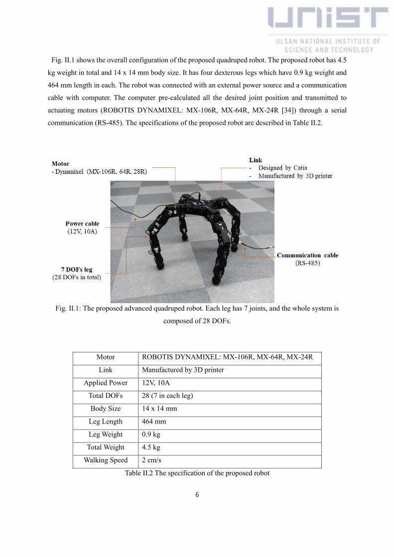
Fig. II.1 shows the overall configuration of the proposed quadruped robot. The proposed robot has 4.5

kg weight in total and 14 x 14 mm body size. It has four dexterous legs which have 0.9 kg weight and

464 mm length in each. The robot was connected with an external power source and a communication

cable with computer. The computer pre-calculated all the desired joint position and transmitted to

actuating motors (ROBOTIS DYNAMIXEL: MX-106R, MX-64R, MX-24R [34]) through a serial

communication (RS-485). The specifications of the proposed robot are described in Table II.2.

Fig. II.1: The proposed advanced quadruped robot. Each leg has 7 joints, and the whole system is

composed of 28 DOFs.

Motor ROBOTIS DYNAMIXEL: MX-106R, MX-64R, MX-24R

Link Manufactured by 3D printer

Applied Power 12V, 10A

Total DOFs 28 (7 in each leg)

Body Size 14 x 14 mm

Leg Length 464 mm

Leg Weight 0.9 kg

Total Weight 4.5 kg

Walking Speed 2 cm/s

Table II.2 The specification of the proposed robot

7

II.2 Kinematic Analysis of one leg

As previously mentioned, each leg of the proposed robot has 7 DOFs as shown in Fig. II.2. The

kinematic relation between the robot's body frame {B} and the end-effector frame {E} was found by

conventional forward kinematics methods such as Denavit-Hartenburg (DH) method. Note that the

geometrical configurations, and the attached reference frames of other legs are all identical. Because

each of the four identical legs has seven rotational actuators to set the position and orientation of the

end-effector, the proposed robot has kinematic redundancy of one that allows flexibility in

manipulations.

Fig. II.2: Attached reference frames on the robot ({B}: the robot’s body frame, {E}: end-effector

frame), z-axis of each joint frames coincides with the rotational axis.

Table II.3 is the DH table of the robot leg in Fig II.2. From the table, the transformation matrix for

each joint can be found by

8

B 1i 1ia id iq

1 b, x -axis -b, y -axis 145 , z -axis 1q

2 90 1L 0 2q

3 90 2L 0 3q

4 90 3L 0 4q

5 90 4L 0 5q

6 90 5L 0 906 q

7 90 6L 0 7q

E 0 7L 0 0

Table II.3: DH table of the single leg.

1

cosαd

sinαd

a

0

cosα

sinα

0

0

sinαcosq

cosαcosq

sinq

0

sinαsinq

cosαsinq

cosq

)q,zRot()d,zTran()a,xTran()α,xRot(T

1ii

1ii

1i

1i

1i

1ii

1ii

i

1ii

1ii

i

ii1i1ii1,-i

(II.1)

Using (II.1), the transformation matrix of the leg’s end-effector from the body frame can be calculated

by

1000

TTTTTTTTT

33

23

13

32

22

12

31

21

11

E7,6,75,64,53,42,31,20,1E0,

z

y

x

P

P

P

R

R

R

R

R

R

R

R

R

(II.2)

In (II.2), zyx P,P,P represent zyx ,, position parameters of the end-effector seen from the body

frame. To represent the orientation of the end-effector, ZYZ Euler angles notation which is one of sets

of Euler angles was used. The rotation described by ZYZ Euler angles is obtained as composition of the

following elementary rotations (Fig. II.3):

9

Fig. II.3: Representation of Euler angles ZYZ [35]

Rotate the reference frame by the angle about axis z .

Rotate the current frame by the angle about axis 'y .

Rotate the current frame by the angle about axis '''z .

In ZYZ Euler angles, the requested solution is, [35]

)(atan2

)(atan2

)atan2(

3132

33

2

23

2

13

1323

R,R

R,RR

R,R

(II.3)

Then, using (II.2) and (II.3), the position and orientation vector of the end-effector with respect to the

body frame can be found by:

)](atan2),(atan2),,(atan2,,,[

][

313233

2

23

2

131323 R,R,RRRRRPPP

zyx

zyx

T

p (II.4)

which is the function of joint values as:

)q,q,q,q,q,q,f(q 7654321p (II.5)

By conducting the time derivative of (II.5), kinematic relationship between velocity vector of end-

effector and joint velocity vector can be found by:

10

qJp

leg

7

6

5

4

3

2

1

7654321

7654321

7654321

7654321

7654321

7654321

q

q

q

q

q

q

q

θ

ψ

θ

ψ

θ

ψ

θ

ψ

θ

ψ

θ

ψ

θ

ψ

θ

θ

θ

θ

θ

θ

θ

θ

θ

θ

θ

θ

θ

θ

θθθθθθθ

θ

z

θ

z

θ

z

θ

z

θ

z

θ

z

θ

z

θ

y

θ

y

θ

y

θ

y

θ

y

θ

y

θ

y

θ

x

θ

x

θ

x

θ

x

θ

x

θ

x

θ

x

(II.6)

where 7x6legJ is the analytic Jacobian matrix of the leg,

7

7654321 ][ Tqqqqqqq q is

the joint velocity vector, 6p is the velocity vector of the end-effector with respect to the body

frame. When the manipulator is redundant, the Jacobian matrix has more columns than rows and infinite

solutions exist to solve the inverse kinematics from (II.6). A viable method to solve such inverse

kinematics problem is to formulate the problem as a constrained linear optimization problem [35].

In detail, the inverse kinematics problem from (II.6) is desired to find the solution q and minimize

the quadratic cost function of joint velocities

qWqq T

2

1)g( (II.7)

where W is a suitable (7 x 7) symmetric positive definite weighting matrix. This problem can be solved

by the method of Lagrange multipliers with the modified cost function

)(2

1),g( qJpλqWqλq

leg

TT (II.8)

where λ is an (6 x 1) vector of unknown multipliers. To minimize the modified cost function, the

requested solution has to satisfy the necessary conditions:

0q

T

g 0

λ

T

g (II.9)

From the first necessary condition, it is 0λJqW T

leg , thus

λJWqT

leg

1 (II.10)

11

where the inverse of W exists. Notice that the solution (II.10) is a minimum since Wq 22 / g is

positive definite. From the second necessary condition, the constraint

qJp leg (II.11)

is calculated. Combining two conditions in (II.10) and (II.11) gives

λJWJpT

legleg

1 (II.12)

Under the assumption that T

legleg JWJ 1 is invertible, solving for λ yields

pJWJλ 11 )( T

legleg (II.13)

which, substituted into (II.10), gives the sought optimal solution,

pJWJJWq 111 )( T

legleg

T

leg (II.14)

II.3 Foot Design

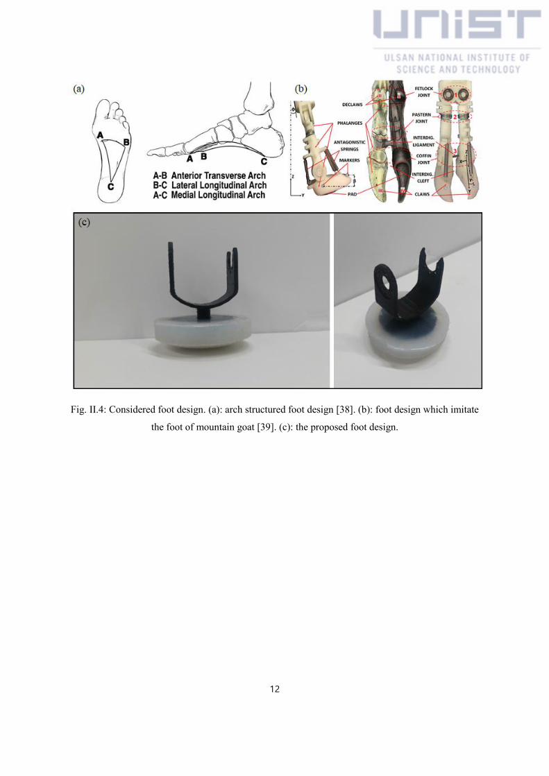
In the case of the foot shape, a sphere-shaped foot was suitable to adapt in a rough terrain, but it made

our robot easy to be tumbled. In [36, 37], the arch structure of human foot as in Fig. II.4-(a) was studied

for stability, and the foot morphology inspired by mountain goat as in Fig. II.4-(b) was studied in [39]

for slip reduction. However, manufactured foot design based on these works did not show huge

performance increment in mobile platform but increase the complexity of the design. Thus, by using

the silicon material named Smooth-on Dragon skin 30 [40], we made curved shape foot to adapt in

rough terrain by changing its own shape while sustaining stability as shown in Fig. II.4-(c)

12

Fig. II.4: Considered foot design. (a): arch structured foot design [38]. (b): foot design which imitate

the foot of mountain goat [39]. (c): the proposed foot design.

13

III. Modified Improved Jacobian Pseudoinverse (mIJP) Algorithm

III.1 Weighted Least Norm (WLN) Method

A differential kinematics is commonly used to control a manipulator since it relates joint space velocity

with a task space velocity through a Jacobain [35, 41]. For each leg, we compute the single-leg Jacobian,

76J , of the foot position with respect to the robot frame as in (II.14). A particular case occurs

when the weighting matrix W is the identity matrix I and the solution simplifies into

pJq (III.1)

where the matrix

1)( TTJJJJ (III.2)

is the Jacobian pseudo-inverse (JP) matrix of J . However, JP method does not consider the physical

limit of each joints of the manipulator. For joint limit avoidance, the joint velocity of a redundant

manipulator is calculated as follows, which is called the weighted least norm (WLN) method [10]:

0)(

if1

0)(

if)(

1

and,

000

000

000

where

)(][

7

2

1

111

i

ii

i

d

TT

q

qqw

w

w

w

qH

qHqH

W

KexJJWJWq

(III.3)

2

min,

2

max,

min,max,

2

min,max,

)()(4

)2()()(

iiii

iiiii

i qqqq

qqqqq

q

qH (III.4)

In (III.3), 7q is the joint position vector,

7q is the joint velocity vector, 6dx is a

desired velocity vector in the task space seen from the body frame, 66K is a positive definite

diagonal matrix, 6e is an error between the end-effector's desired position and the current

14

position, 77W is the weighting matrix and iw is the weighting factor of joint i . Also, to

exploit the redundancy of the leg,

iq

)(qH is defined as (III.4) so that the joints are forced to stay

within their limits, where iq is current position of joint i , and max,iq and

min,iq are its maximum

and minimum position, respectively. Fig. III.1 is the simulation results of the WLN method when the

manipulator was commanded to follow exactly same trajectory in Fig. III.1-(a) and (b). By comparing

two results, we could verify that the WLN method ensure the joint limit avoidance of the manipulator.

Fig. III.1: Joint values during trajectory following. (a). joint values without WLN method. (b). joint

values with WLN method.

III.2 Improved Jacobian Pseudoinverse (IJP) Algorithm

One can measure the distance from a singularity of a (redundant) manipulator at current posture using

a condition number (CN) of the Jacobian, )( J , as below [42].

)(

)()(

min

max

J

JJ

(III.5)

In (III.5), max and min are the maximum and minimum singular values of the Jacobian J ,

15

obtained from singular value decomposition respectively. Using a JP algorithm with WLN method of

(III.3) can generate a desired trajectory accurately as long as the condition number is small. However,

it shows a large error when the condition number is large. For example, Fig. III.2-(a) shows the

calculated trajectory of the robot’s leg using (III.3) when its condition number at initial posture is 6.03,

and the corresponding error is almost zeros as shown in Fig. III.2-(b). On the other hand, condition

number at the initial posture in Fig. III.2-(c) is 10156, and incurs a large error at the early stage of the

trajectory as shown in Fig. III.2-(d).

To reduce the sharp error peak, Improved Jacobian Pseudoinverse (IJP) algorithm was proposed in [17]

using 6 DOFs leg. The key idea is calculating again the given trajectory in reverse order after finishing

the calculation in forward direction. The detailed steps are described as follows:

STEP0: Check whether the CN of the leg at initial posture is bigger than a threshold 1 . If CN > 1 ,

go to the STEP1, whereas if CN < 1 , calculate joint position as usual using (III.3) and done.

STEP1: For a given desired trajectory dx and an initial joint position initq , calculate the last joint

position endq at the end of dx using (III.3).

STEP2: Obtain revd ,x by reversing dx , and calculate the series of joint positions in reverse order

revq from revd ,x start from endq using (III.3). Note that endq is now the initial joint position of

revd ,x .

STEP3: Reverse revq and obtain q , which is a series of joint positions to smoothly follow dx

with a reduced error at the early stage of dx .

STEP4: While calculating revq in STEP2, if CN at the beginning of revd ,x is higher than threshold

2 (equivalently, if the CN at the end of dx is higher than 2 ), then calculate again only the last

part of q start from a corresponding point in dx .

By using the IJP algorithm, we could minimize the error as shown in Fig. III.2-(f) when the leg was

commanded to follow the exactly same trajectory as in Fig. III.2-(c).

16

Fig. III.2: Simulation results of the inverse kinematics of the robot’s leg and the corresponding error

with different values of condition numbers. (a) and (b) : initial condition number is 6.03, and JP with

WLN is used, (c) and (d) : initial condition number is 10156, and JP with WLN is used, (e) and (f) :

initial condition number is 10156, and IJP with WLN is used.

17

III.3 Modified Improved Jacobian Pseudoinverse (mIJP) Algorithm

In the IJP algorithm, to calculate the trajectory in reverse order, the calculated final position of the

leg’s end-effector is required to be coincided with the desired position. However, by considering the

orientation of the end-effector, the redundancy of the leg decreased from three to one (from 6 DOFs

with position parameters to 7 DOFs with position and orientation parameters), which makes difficult to

satisfy this required condition when the CN of an initial posture is large. For example, Fig. III.3 shows

simulation results of the inverse kinematics of the robot's legs using (III.3) when the CN is 6129, which

is near the singularity. Fig. III.3-(a) and (c) are the results when the JP with WLN method was used.

Because the calculated result does not converge to desired position, it is impossible to calculate the

trajectory in reverse order which is the first step of the IJP algorithm.

Therefore, we modified the IJP algorithm to reduce errors without any requirement even when the CN

is large. The idea is to calculate the joint angles of the final position of the trajectory not from the current

position, but an arbitrary non-singular posture. From the arbitrary non-singular posture, a virtual

trajectory is generated to the final position. Since the virtual trajectory starts from the small CN, it

converges to the final position even with the reduced redundancy. After calculating the final joint angles,

we can calculate the given trajectory in reverse order as the remaining steps of the previous IJP

algorithm.

By using the mIJP algorithm, we could minimize the error without the required condition as shown

in Fig. III.3-(b) and (d) when the leg is commanded to follow the exactly same trajectory as in Fig. III.3-

(a). Note that all the joints are always within their physical limits during the simulations due to the WLN

method. The mIJP algorithm shows the great performance until the length of the trajectory is down to

1.5 mm. Since the length of the single leg is 464 mm, the mIJP algorithm can be said to be valid in the

whole workspace of the manipulator.

18

Fig. III.3: Simulation results of the inverse kinematics of the robot’s leg and the corresponding error

with the condition number of 6129. (a) and (c) : trajectory tracking using JP with WLN, (b) and (d)

trajectory tracking using mIJP with WLN.

19

IV. A COG Trajectory Planning Method

IV.1 Walking Mechanism

For the walking of a robot, there are two walking mechanisms, the first one is the static walking, and

the second one is the dynamic walking. In the static walking, for the stability, the projection of the COG

on the ground should be inside of foot support area as shown in Fig. IV.1.

Fig. IV.1: Static walking [43]

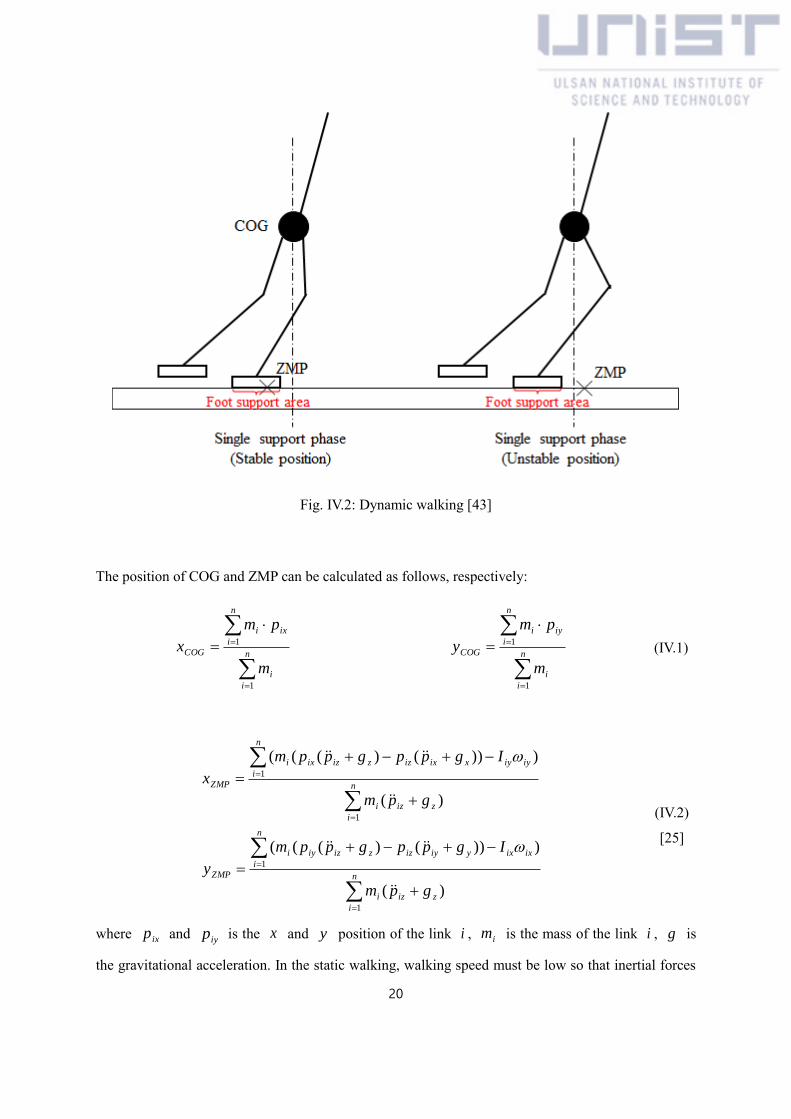
However, in the dynamic walking, the projection of the COG can be outside of the support area, but the

ZMP cannot, as shown in Fig. IV.2.

20

Fig. IV.2: Dynamic walking [43]

The position of COG and ZMP can be calculated as follows, respectively:

n

i

i

n

i

ixi

COG

m

pm

x

1

1

n

i

i

n

i

iyi

COG

m

pm

y

1

1 (IV.1)

n

i

zizi

n

i

ixixyiyizziziyi

ZMP

n

i

zizi

n

i

iyiyxixizzizixi

ZMP

gpm

Igppgppm

y

gpm

Igppgppm

x

1

1

1

1

)(

)))()(((

)(

)))()(((

(IV.2)

[25]

where ixp and iyp is the x and y position of the link i , im is the mass of the link i , g is

the gravitational acceleration. In the static walking, walking speed must be low so that inertial forces

21

are negligible. On the other hands, the dynamic walking can have fewer legs than static machines, and

are potentially faster. Even though the dynamic walking can generate more natural motion of the robot

than the static walking, it requires precise knowledge of robot dynamics which complicated. Many

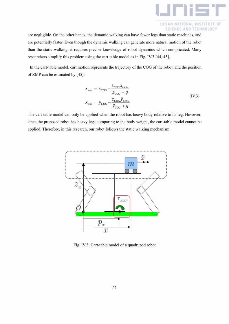
researchers simplify this problem using the cart-table model as in Fig. IV.3 [44, 45].

In the cart-table model, cart motion represents the trajectory of the COG of the robot, and the position

of ZMP can be estimated by [45]:

gz

yzyx

gz

xzxx

COG

COGCOG

COGzmp

COG

COGCOG

COGzmp

(IV.3)

The cart-table model can only be applied when the robot has heavy body relative to its leg. However,

since the proposed robot has heavy legs comparing to the body weight, the cart-table model cannot be

applied. Therefore, in this research, our robot follows the static walking mechanism.

Fig. IV.3: Cart-table model of a quadruped robot

22

IV.2 Stability Criteria

For the static walking, the way to address stability is to examine the SP which is the minimum area

convex point set in the support plane such that all the leg contact points are contained. As long as the

projection of the COG lies in the SP, the robot is statically stable [46] as in Fig. IV.4.

In order to get a robust plan, numbers of stability criteria have been defined, such as, stability margin

(SM) [46], longitudinal stability margin (LSM) [48], energy stability margin (ESM) [49], normalized

energy stability margin (NESM) [50]. Among these criteria, LSM is commonly used because it is

intuitive and easy to calculate. Therefore, we decided to follow LSM criterion as in Fig. IV.5. When the

LSM is greater than zero, then the robot is in a statically stable posture.

Fig. IV.4: Stance posture of the proposed robot. (a): Unstable posture, (b): Stable posture

23

Fig. IV.5: Definitions of longitudinal stability margin: LSM = min(Srm, Sfm)

IV.3 Gait Sequence

To form a SP for a quadruped static walking, only one leg can swing at a time. In this condition, there

are total six possible leg sequences as in Fig. IV.6, but only one sequence satisfies the requirement that

makes the COG to move forward at all times [46, 47]. This sequence is [Right-Hind (RH), Right-

Forward (RF), Left-Hind (LH), Left-Forward (LF)] or [LH, LF, RH, RF] which is gait sequence in Fig.

IV.6-(b). Therefore, we chose this pattern for static walk operation.

Fig. IV.6: A quadruped robot static walking gait sequences start with leg 1

24

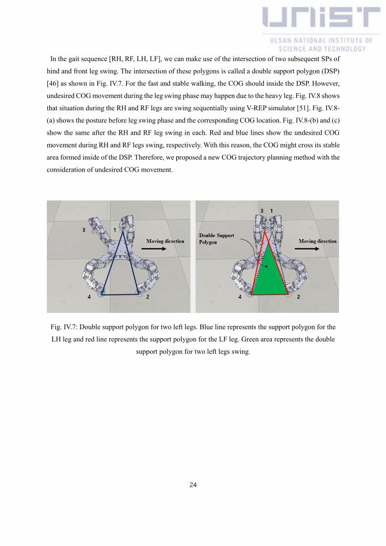
In the gait sequence [RH, RF, LH, LF], we can make use of the intersection of two subsequent SPs of

hind and front leg swing. The intersection of these polygons is called a double support polygon (DSP)

[46] as shown in Fig. IV.7. For the fast and stable walking, the COG should inside the DSP. However,

undesired COG movement during the leg swing phase may happen due to the heavy leg. Fig. IV.8 shows

that situation during the RH and RF legs are swing sequentially using V-REP simulator [51]. Fig. IV.8-

(a) shows the posture before leg swing phase and the corresponding COG location. Fig. IV.8-(b) and (c)

show the same after the RH and RF leg swing in each. Red and blue lines show the undesired COG

movement during RH and RF legs swing, respectively. With this reason, the COG might cross its stable

area formed inside of the DSP. Therefore, we proposed a new COG trajectory planning method with the

consideration of undesired COG movement.

Fig. IV.7: Double support polygon for two left legs. Blue line represents the support polygon for the

LH leg and red line represents the support polygon for the LF leg. Green area represents the double

support polygon for two left legs swing.

25

Fig. IV.8: The undesired COG movement during the RH and RF legs are swing sequentially: (a)

before leg swing phase. (b) after RH leg swing. (c) after RF leg swing. Red and blue lines represent

the COG movement during first and second leg swing, respectively.

IV.4 A COG Trajectory Planning Method

For the COG shift, calculation from the global frame was needed because the body frame moved as

the body moved. However, to use the global frame, the additional devices such as camera are needed to

detect the position of the robot from the global frame. One way to conduct the calculation in the body

frame is to give the same trajectory to all legs with contacting the ground. Then the corresponding body

trajectory will be the reverse of the leg’s trajectory as shown in Fig. IV. 9-(a). However, since the weight

of the proposed robot does not concentrate on the body, the body movement does not fully mean the

COG movement. For example, even though we shift the body by amount of the blue arrow, the

corresponding COG movement will not be the same with the blue arrow like green arrow in Fig. IV.9-

(a). To solve this problem, with the short length shifting of the body, the COG position is checked and

recalculate the direction to move toward the desired position. By repeating this step, if the COG

coincides with the desired point, the COG shift is stopped as shown in Fig. IV.9-(b). However, it requires

26

large computational costs.

Therefore, to conduct the calculation in the body frame with low computational costs, we used

combined Jacobian of the COG and centroid [17] which relates the velocity difference between the

COG and the centroid seen from the body frame with the joint velocity as in Fig. IV.10 and follows:

centS PPP COG (IV.4)

AllSS qJP (IV.5)

Fig. IV. 9: The COG shift methods. (a): Give the same trajectory to all legs with contacting the

ground. (b): with the short length shifting, get the feedback of the direction of the body shift.

Fig. IV.10: The proposed position difference vector between the COG and centroid

27

where 3COGP and

3

cent P are the position vectors of the robot’s COG and the centroid of

the SP viewed from the body frame in each, 28Allq is a joint velocity vector of the whole body,

and 283SJ . Note that COGP and centP in the body frame can be easily found using the forward

kinematics. In similar manner as (III.3), a joint velocity vector of the whole body Allq can be found:

)(][ ,

111edS

T

SAllS

T

SAllAll KPJWJJWq (IV.6)

where 2828AllW is the weighting matrix of whole joints,

3

, dSP is a time derivative of

desired SP , and by letting dS ,P as the desired point, we can easily shift the COG to desired point.

However, without constraint for foot contact points, our method changes the foot contact points instead

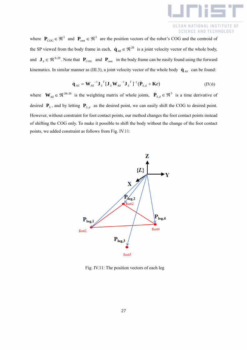
of shifting the COG only. To make it possible to shift the body without the change of the foot contact

points, we added constraint as follows from Fig. IV.11:

Fig. IV.11: The position vectors of each leg

28

constantjleg,ileg, PP (IV.7)

0jleg,ileg, PP (IV.8)

where 3

ileg, P and 3

jleg, P are the position vectors of end-effector of leg i and j viewed

from the body frame, 3

ileg, P and 3

jleg, P are time derivative of ileg,P and

jleg,P . In joint

space expression, (IV.8) can be expressed as:

0

q

q

q

q

JJ

JJ

JJ

4,

3,

2,

1,

4,3,

3,2,

2,1,

00

00

00

leg

leg

leg

leg

legleg

legleg

legleg

(IV.9)

where 7

ileg, q is joint values of leg i , 73

ileg,

J is the Jacobian matrix of the leg i . At this

point, rearrange the 28 joints into the actuated and passive joints. Then, (IV.9) can be rearranged as:

0q

qHH

p

a

pa

(IV.10)

where aq and pq are joint velocities of actuated and passive joints, aΗ and

pΗ are collection

of columns of the actuated and passive joints, respectively. To make use of redundancy in both actuated

and passive joints, the number of actuated joints should be greater than 3 which is the dimension of the

velocity vector, and the number of passive joints should be greater than the number of actuated joints.

Therefore, the possible numbers of actuated joints for each leg are 1,2,3. With the assumption that three

joints are actuated joint for each leg, the relationship between the actuated and passive joints can be

expressed as:

aapp qHHq (IV.11)

where 12aq and

16pq , 129aH and

169pH . 916

pH is a pseudo-

inverse of pH . With this constraint, (IV.5) is rearranged to:

aCa

ap

SAllSS qJqHH

IJqJP

12 (IV.12)

where 28][ T

paAll qqq , and 123CJ . To exploit the redundancy for joint limit avoidance,

the velocity vector of actuated joints can be derived as:

29

dS

T

CaC

T

Caa ,

111][ PJWJJWq

(IV.13)

where 1212aW is the weighting matrix of the actuated joint from AllW in (IV.6). In similar

manner, velocity vector of the passive joint in (IV.11) is rearranged to:

aa

T

ppp

T

ppp qHHWHHWq 111][

(IV.14)

where 1616pW is the weighting matrix of the passive joint from AllW in (IV.6).

Fig. IV.12 shows the simulation results when the robot was commanded to coincide its COG with the

figure-8 trajectory. The COG trajectory and the corresponding foot contact points were shown without

constraint in Fig. IV.12-(a) and with constraint in Fig. IV.12-(b). It shows better performance for

tracking the desired trajectory and maintaining the foot contact point when the constraint in (IV.7) and

(IV.8) was applied. Even though errors still exist due to the foot slippage, but they are not significant

enough to influence the stability of the robot.

30

Fig. IV.12: The robot was commanded to coincide its COG to the figure-8 trajectory in simulation.

The position of the COG and supporting feet are marked. (a) and (c): without the constraint for foot

contact point, (b) and (d): with the constraint for foot contact point.

By using (IV.13) and (IV.14), the proposed COG trajectory planning method shifts the COG to the

point where the COG is always inside the DSP even with the undesired COG movement during the leg

swing phase. Also, by removing unnecessary shift motion of the body, our method enables efficient

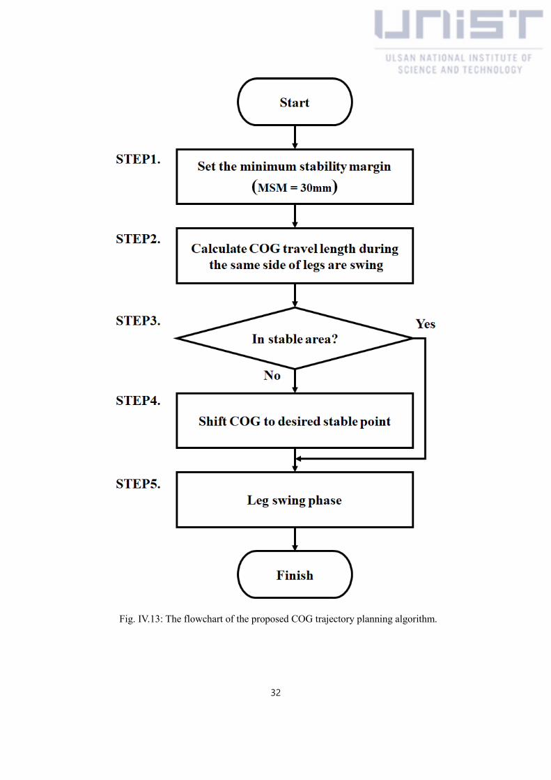
walking of the robot. The detailed steps are described as follows (Fig. IV.13):

STEP1: In order to ensure stability of the actual robot, a minimum stability margin (MSM) is

necessary. The robot is stable only when LSM is greater than MSM. For our platform, we set MSM as

30mm by considering the robot size.

31

STEP2: Kinematically calculate the COG travel distance (CTD) from Fig. IV.8-(a) to Fig. IV.8-(c)

without actual movement.

STEP3: Check if the COG is in the stable area or not. If the whole COG trajectory is in stable area

during the leg swing phase, move to STEP5. If not, move to STEP4.

STEP4: With the calculated CTD, the goal of this step is to shift the COG to the stable area with the

consideration of the undesired COG movement. For example, Fig. IV.14 shows the COG shift plan

before two right-side legs swing. At the initial posture in Fig. IV.14-(a), the robot is unstable as shown

in Fig. IV.14-(b). If we shift the COG from Fig. IV.14-(b) to (c), the robot is stable, but it is inefficient

because of the excessive transversal movement. Therefore, our goal is to shift the COG from Fig. IV.14-

(b) to (d) for stable and efficient walking.

STEP5: Move the leg to the swing phase.

32

Fig. IV.13: The flowchart of the proposed COG trajectory planning algorithm.

33

Fig. IV.14: COG shift plan before two right-side legs swing. The red line is SP before RH leg swing

and the blue line is SP before RF swing. The green line is stable area where LSM is ensured to be

greater than MSM inside DSP. (a) Initial posture before leg swing when the robot tends to move left

direction. (b) COG location of initial posture. The robot is unstable. (c) Stable but inefficient COG

location because unnecessary shift motion exists. (d) Stable and efficient COG location.

34

V. Performance verification by Simulations and Experiments

V.1 Simulation Results

To verify the performance of the proposed robot and the algorithms, the V-REP simulator was used in

this work. First, we simulated the robot to walk forward with the proposed algorithm as shown in Fig.

V. 1. With the gait sequence [RH, RF, LH, LF], from initial posture in take 1, shifted the COG in take2,

swung RH and RF legs in take3-4, shifted the body forward in take5, shifted COG in take6, LH and LF

legs swung in take7-8, shifted the body forward in take9. The mIJP algorithm was applied every time

when the robot tried to swing its leg. At the same time, the robot coincided its COG to the point where

stable and efficient walking was guaranteed as shown in Fig. IV.14-(d) using (IV.13) and (IV.14). Fig.V.2

shows COG movement during two right side legs swing phase and the corresponding SPs. The red line

is the SP before RH leg swing, and the blue line is the SP before RF leg swing (after RH leg swing). By

putting the CTD to the stable area, stable and efficient walk was ensured.

Also, the robot could change its height up to 180% from initial posture by giving the same trajectory

to all legs toward vertical axis as shown in Fig. V.3. Even though there was an obstacle in the moving

direction, the robot could easily overcome by changing its height. The walking algorithm was the same

with the previous one in Fig. V.1.

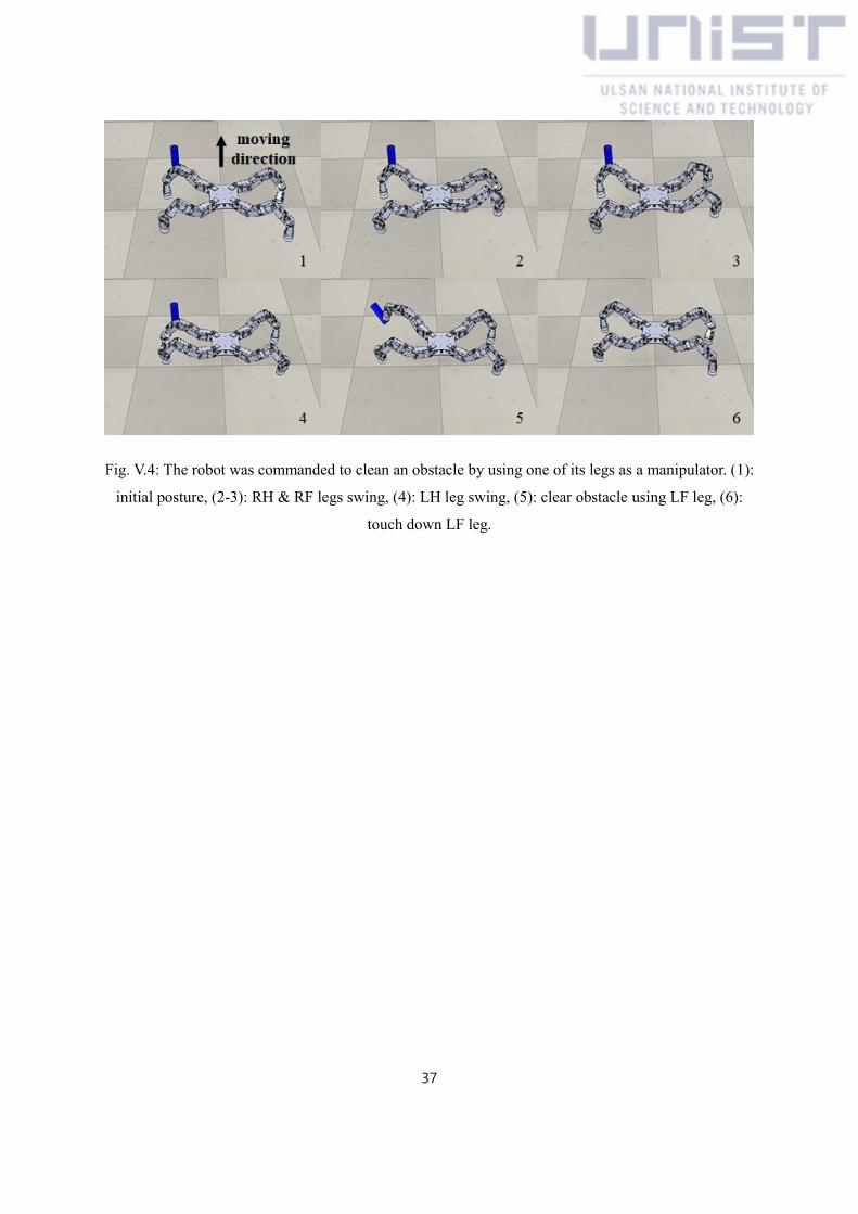
In Fig. V.4, we simulated the robot to clean an obstacle by considering the situation that the robot uses

its leg as a manipulator. Before raising the leg, we commanded the robot to move its COG inside the SP

formed by the remaining three feet using (IV.13) and (IV.14).

Not only traveling on the flat terrain, but also the robot could pass through narrow gap down to 40 cm

(initial width = 70 cm) with different posture as shown in Fig. V.5. Instead of common walking, the

robot passed through narrow gap with crawl gait like caterpillar. From the initial posture in take1, the

robot lifted and shifted the body forward in take2. In take3-4 the robot lifted and shifted the legs forward.

In this gait, body contacted the ground except take2. Therefore, we did not have to consider the stability

of the robot.

35

Fig. V. 1: Snapshots of the robot during the simulation. (1): initial posture, (2): COG shift, (3-4): RH

& RF legs swing, (5-6): COG shift, (7-8): LH & LF legs swing, (9): back to initial posture.

36

Fig. V. 2: Simulation results when the robot was commanded to walk on the plain terrain. The red line

is the SP before first leg (RH) swing and the blue line is the SP before second leg (RF) swing. The red

circle represents undesired COG movement during first leg swing, and the blue circle represent that of

second leg swing. The green line is the stable area where LSM is guaranteed to be greater than MSM

inside DSP.

Fig. V.3: The robot could change its height up to 180% from initial posture to avoid the obstacle in the

moving direction. (1): initial posture, (2): change height, (3-4): RH & RF legs swing, (5-6): LH & LF

legs swing.

37

Fig. V.4: The robot was commanded to clean an obstacle by using one of its legs as a manipulator. (1):

initial posture, (2-3): RH & RF legs swing, (4): LH leg swing, (5): clear obstacle using LF leg, (6):

touch down LF leg.

38

Fig. V.5: The robot could overcome narrow gap by changing its posture. (1): initial posture, (2): lift

and shift the body forward, (3-4): lift and shift the legs forward.

V.2 Experimental Results

In the experiment, the robot was in the same situation with the simulation in section V.1. First, the

robot was commanded to walk forward as in Fig. V.1 with the proposed algorithm. In Fig.V.6, after the

robot shift the COG to ensure stable and efficient walking, swung the RH and RF legs from the take1-

4. The same procedures were repeated for left legs in take5-8. The robot could traverse 13 cm forward

in a single cycle of walking, and the walking speed is about 2 cm/s, A statically stable gait was achieved

using the proposed algorithm.

The height change during walking was also verified in the experiment. In Fig. V.7, the obstacle with

12.5 cm height (robot height = 8.5 cm) was set at the front of the robot. Instead of circumventing the

39

obstacle, the robot could easily overcome by changing its height. After changing its height in take1-2,

take3-6 show the same walking algorithm of Fig. V.3.

Also, the robot was tested to clean an obstacle as shown in Fig. V.8. The robot located its COG inside

the SP formed by the remaining three feet using (IV.13) and (IV.14). This test showed that the robot can

do a simple task by using its leg as a manipulator.

Lastly, the robot passed through narrow gap by changing its posture. In Fig. V.9, narrow gap was set

to 45 cm. The robot lifts and shifts the body forward in take1-2, lift and shift the legs forward in take3-

4.

Fig. V.6: The robot took a step forward as in Fig. V.1. (1): initial posture, (2): COG shift, (3-4): RH \&

RF legs swing, (5-6): COG shift, (7-8): LH \& LF legs swing, (9): back to initial posture

40

Fig. V.7: The robot changed its height as in Fig. V.3. (1): initial posture, (2): change height, (3-4): RH

& RF legs swing, (5-6): LH & LF legs swing.

Fig. V.8: The robot cleared the obstacle as in Fig. V.4. (1): initial posture, (2-3): RH & RF legs swing,

(4): LH leg swing, (5): Clear obstacle using LF leg, (6): touch down LF leg.

41

Fig. V.9: The robot passed through narrow gap as in Fig. V.5. (1): initial posture, (2): lift and shift the

body forward, (3-4): lift and shift the legs forward.

42

VI. Conclusion and Open Issues

In this thesis, a redundant quadruped robot that has 28 degree-of-freedoms (DOFs) (7 DOFs in one

leg) was proposed for various types of locomotion and manipulation. Inverse kinematics of each leg,

which has 7 joints, was handled by the modified improved Jacobian pseudoinverse (mIJP) algorithm

together with the weighted least norm (WLN) method which forces all joints in their physical limits.

Previously, the improved Jacobian pseudoinverse (IJP) algorithm was proposed to generate accurate

trajectory following even when the initial posture of the leg is close to the singularity. The IJP algorithm

requires the calculated final position of the leg to be coincided with the desired position. However, with

the decrease of redundancy, it became difficult to satisfy this required condition. Therefore, the mIJP

algorithm was proposed to accurately follow trajectory even with the decreased number of redundancy.

This mIJP algorithm with the WLN method was used to follow a desired trajectory of the leg in this

thesis.

In addition, to maintain a statically stable posture when the robot walks, a combined Jacobian of center

of gravity (COG) and a centroid of the support polygon (SP) with the constraints for the foot contact

points was proposed. This method helped the robot to shift the COG to desired position with reduced

errors and made it possible to all calculations are conducted in the body frame. With this method, a

COG trajectory planning method for stable and efficient walk was proposed. In the case of the

quadruped robot which has heavy legs, undesired COG movement occurs during leg swing phase. By

shifting the undesired COG movement to the stable area, stable and efficient walking could be achieved.

The proposed methods were verified in simple walking, changing height, clearing obstacle, and passing

through narrow gap. All these scenarios were verified by simulations and experiments.

However, to detect obstacle and travel rough terrain, sensory feedbacks (e.g., Inertia Measurement

Unit, force sensor, camera sensor) are needed. Hence, adding some sensors in the robot to boost the

performance in more complex environment is needed. Also, dynamics of the robot should be considered.

Even though the proposed robot shows versatile mobility in various environments, walking ability on

the plain terrain was below expectation. By considering the dynamics of the robot, movement speed

should be increased. Additionally, computations and controls of the robot should be handled by an on-

board processor to reduce the communication delay between the robot and computer.

43

REFERENCE

[1] M. Cianchetti, M. Calisti, L. Margheri, M. Kuba, and C. Laschi, “Bioinspired locomotion and

grasping in water: the soft eight-arm OCTOPUS robot,” Bioinspiration & Biomimetics, vol. 10, no. 3,

2015.

[2] M. Sfakiotakis, A. Kazakidi, A. Chatzidaki, T. evdaimon, and D. P. Tsakiris, “Multi-arm Robotic

Swimming with Octopus-inspired Compliant Web,” IEEE International Conference on Intelligent

Robots and Systems (IROS), 2014, pp. 302-308

[3] A. Shkolnik and R. Tedrake, “Inverse kinematics for a point-foot quadruped robot with dynamic

redundancy resolution,” in IEEE International Conference on Robotics and Automation, 2007, pp.

4331– 4336.

[4] D. Pongas, M. Mistry, and S. Schaal, “A robust quadruped walking gait for traversing rough terrain,”

in IEEE International Conference on Robotics and Automation, 2007, pp. 1474–1479.

[5] B. del Rosario, C. S. Falcon, J. P. Pasion, and F. Tamonte, “Implementation of Balance Control on

Terrain Quadruped Traversal” in IEEE International Conference Humanoid, Nanotechnology,

Information Technology, Communication and Control, Environment and Management, 2015, pp. 1-5.

[6] S. Kitano, S. Hirose, A. Horigome, and G. Endo, “TITAN-XIII: sprawling-type quadruped robot

with ability of fast and energy-efficient walking,” ROBOMECH Journal, vol. 3, no. 1, pp. 8-23, 2016.

[7] K. Byl, M. Byl, and B. Satzinger, “Algorithmic optimization of inverse kinematics tables for high

degree-of-freedom limbs,” in Proc. ASME Dynamic Systems and Control Conference (DSCC), 2014.

[8] B. W. Satzinger, J. I. Reid, M. Bajracharya, P, Hebert, and K. Byl, “More Solution Means More

Problems: Resolving Kinematic Redundancy in Robot Locomotion on Complex Terrain,” in IEEE

Intelligent Robots and Systems (IROS), 2014, pp. 4861-4867.

[9] S. Chiaverini, G. Oriolo, and I. D. Walker, Kinematically redundant manipulators. Springer

Handbook of Robotics (ed. Bruno Siciliano and Oussama Khatib). Springer, 2008.

[10] T. F. Chan and R. V. Dubey, “A weighted least-norm solution based scheme for avoiding joint

limits for redundant joint manipulators,” IEEE Transactions on Robotics and Automation, vol. 11, no.

2, pp. 286–292, 1995.

44

[11] L. Sciavicco and B. Siciliano, “A solution algorithm to the inverse kinematic problem for redundant

manipulators,” IEEE Journal on Robotics and Automation, vol. 4, no. 4, pp. 403–410, 1988.

[12] S. B. Slotine, “A general framework for managing multiple tasks in highly redundant robotic

systems,” in International Conference on Advanced Robotics, vol. 2, 1991, pp. 1211–1216.

[13] A. Colomn and C. Torras, “Closed-loop inverse kinematics for redundant robots: Comparative

assessment and two enhancements.” IEEE/ASME Transactions on Mechatronics, vol. 20, pp. 944-955,

2015

[14] A. A. Goldenberg, B. Benhabib, and R. G. Fenton, “A complete generalized solution to the inverse

kinematics of robots,” IEEE Journal of Robotics and Automation, vol. RA-1, pp. 14-20, 1985.

[15] D. Omrcen, L. Zlajpah, and B. Nemec, “Compensation of velocity and/or acceleration joint

saturation applied to redundant manipulator,” Robotics and Autonomous Systems, vol. 55, pp. 337–344,

2007.

[16] F. Flacco, A. D. Luca, and O. Khatib, “Motion control of redundant robots under joint constraints:

Saturation in the null space,” in IEEE International Conference on Robotics and Automation, 2012, pp.

285–292.

[17] B. Kwak, H. Park, and J. Bae, “Development of a quadruped robot with redundant dofs for high-

degree of functionality and adaptation,” in IEEE International Conference on Advanced Intelligent

Mechatronics (AIM), 2016, pp. 608–613.

[18] F.-T. Cheng, H.-L. Lee, and D. E. Orin, “Increasing the locomotive stability margin of multilegged

vehicles,” in IEEE International Conference on Robotics and Automation, vol. 3, 1999, pp. 1708–1714.

[19] D. Pongas, M. Mistry, and S. Schaal, “A robust quadruped walking gait for traversing rough terrain,”

in IEEE International Conference on Robotics and Automation, 2007, pp. 1474–1479.

[20] S. Zhang, X. Rong, Y. Li, and A. B. Li, “A composite cog trajectory planning method for the

quadruped robot walking on rough terrain,” International Journal of Control and Automation, vol. 8,

no. 9, pp. 101–118, 2015.

[21] A. Shkolnik and R. Tedrake, “Inverse Kinematics for a Point-Foot Quadruped Robot with Dynamic

Redundancy Resolution,” IEEE International Conference on Robotics and Automation, 2007, pp. 4331-

4336

45

[22] M. Mistry, J. Nakanishi, G. Cheng, and S. Schaal, “Inverse Kinematics with Floating Base and

Constraints for Full Body Humanoid Robot Control,” IEEE/RAS International Conference on

Humanoid Robots, 2008, pp. 22-27

[23] M. Mistry, J. Nakanishi, and S. Schaal, “Task Space Control with Prioritization for Balance and

Locomotion,” IEEE/RSJ International Conference on Intelligent Robots and Systems, 2007, pp.331-

338

[24] V. Loc, I. Koo, D. T. Tran, S. Park, H. Moon, and H. Choi, “Body Workspace of Quadruped

Walking Robot and its Applicability in Legged Locomotion,” Journal of Intelligent and Robotic

Systems, 2012, vol 67, pp. 271-284

[25] M. Vukobratovic and B. Borovac, “Zero-moment point: Thirty five years of its life,” Internatioanl

Journal of Humanoid Robotics, vol. 1, pp. 157–173, 2004.

[26] K. Byl and M. Byl, “Design of fast walking with one- versus twoat-a-time swing leg motions for

robosimian,” in IEEE International Conference on Technologies for Practical Robot Applications, 2015,

pp. 1–7.

[27] M. Kalakrishnan, J. Buchli, P. Pastor, M. Mistry, and S. Schaal, “Fast, robust quadruped

locomotion over challenging terrain,” in IEEE International Conference on Robotics and Automation,

2010, pp. 2665–2670.

[28] G. Z. Lum, S. K. Mustafa, H. R. Lim, W. B. Lim, G. Yang, and S. H. Yeo, “Design and Motion

Control of a Cable-driven Dexterous Robotic Arm,” IEEE Conference on Sustainable Utilization and

Development in Engineering and Technology, 2010, pp. 106-111.

[29] G. Yang, S. K. Mustafa, S. H. Yeo, W. Lin, and W. B. Lim, “Kinematic design of an

anthropomimetic 7-DOF cable-driven robotic arm,” Frontiers of Mechanical Engineering, vol. 6, pp.

45-60, 2011.

[30] F. Renda, M. Giorelli, M. Calisti, M. Cianchetti, and C. Laschi, “Dynamic Model of a

Multibending Soft Robot arm Driven by Cables,” IEEE Transaction on Robotics, 2014, pp. 1109-

1122

[31] J. Tian and Q. Lu, “Simulation of Octopus Arm Based on Coupled CPGs,” Journal of Robotics,

vol. 4, 2015.

46

[32] M. V. Damme, F. Daerden, and D. Lefeber, “A Pneumatic Manipulator used in Direct Contact

with an Operator,” IEEE International Conferenct on Robotics and Automation, 2005, pp. 4494-

4499.

[33] KINOVA. (2017) JACO 7DOF-S. [Online]. Available: http://www.kinovarobotics.com/

[34] ROBOTIS. (2017) Dynamixel. [Online]. Available: http://www.robotis.com/

[35] B. Siciliano, L. Sciavicco, L. Villani, and G. Oriolo, Robotics: Modeling, Planning and Control.

Springer, 2009.

[36] R. F. Ker, M. B. Bennett, S. R. Bibby, R. C. Kester, and R. M. Alexander, “The spring in the arch

of the human foot,” Nature, vol. 325, pp. 147-149, 1987.

[37] E. Anzai, K. Nakajima, Y. Iwakami, M. Sato, S. Ino, T. Ifukube, K. Yamashita, and Y. Ohta,

“Effects of Foot Arch Structure on Postural Stability,” Clinical Research on Foot and Ankle, vol. 2,

2014

[38] H. Gray, Anatomy of the Human Body. C. M. Goss, Ed. Philadelphia, PA: Lea and Febiger, 1949

[39] S. A. Abad, N. Sornkarn, and T. Nanayakkara, “The Role of Morphological Computation of the

Goat Hoof in Slip Reduction,” IEEE International Conference on Intelligent Robots and Systems, 2016,

pp. 5599-5605.

[40] SMOOTH-ON. (2017) Dragon skin. [Online]. Available: https://www.smooth-on.com/product-

line/dragon-skin/

[41] D. E. Whitney, “Resolved motion rate control of manipulators and human prostheses,” IEEE

Transactions on man-machine systems, vol. 10, no. 2, pp. 47–53, 1969.

[42] J. P. Merlet, “Jacobian, Manipulability, Condition Number, and Accuracy of Parallel Robots,”

Journal of Mechanical Design, vol. 128, no. 1, pp. 199-206, 2005

[43] E. Cuevas, D. Zaldivar, and R. Rojas, “Bipedal robot description,” Technical Report B-03-19, 2004.

[44] S. Kajita, F. Kanehiro, K. Kaneko, K. Fujiwara, K. Harada, K. Yokoi, and H. Hirukawa, “Biped

Walking Pattern Generation by using Preview Control of Zero-Moment Point,” IEEE International

Conference on Robotics and Automation, 2003, pp. 1620-1626.

[45] A. W. Winkler, C. Mastalli, I. Havoutis, M. Foucchi, D. G. Caldwell, and C. Semini, “Planning

and Execution of Dynamic Whole-Body Locomotion for Hydraulic Quadruped on Challenging Terrain,”

IEEE International Conference on Robotics and Automation, 2015, pp. 5148-5154.

47

[46] R. B. McGhee and A. A. Frank, “On the stability properties of quadruped creeping gaits,”

Mathematical Biosciences, vol. 3, pp. 331–351, 1968.

[47] D. J. Pack and A. C. Kak, “A Simplified Forward Gait Control for a Quadruped Walking Robot,”

IEEE Intelligent Robots and Systems, 1994, pp. 1011-1017.

[48] S.-M. Song and K. J. Waldron, “An analytical approach for gait study and its applications on wave

gaits,” The International Journal of Robotics Research, vol. 6, no. 2, pp. 60–71, 1987.

[49] D. Messuri and C. Klein, “Automatic body regulation for maintaining stability of a legged vehicle

during rough-terrain locomotion,” IEEE Journal on Robotics and Automation, vol. 1, no. 3, pp. 132–

141, 1985.

[50] S. Hirose, H. Tsukagoshi, and K. Yoneda, “Normalized energy stability margin and its contour of

walking vehicles on rough terrain,” in IEEE International Conference on Robotics and Automation, vol.

1, 2001, pp. 181–186.

[51] Coppelia Robotics. (2017) V-REP. [Online]. Available: http://www.coppeliarobotics.com/