Human Mobility and Spatial Disease Dynamics

Dirk Brockmann1, Vincent David1,2 and Alejandro Morales Gallardo1,2

1Engineering Sciences and Applied Mathematics, NorthwesternUniversity, 2145 Sheridan Rd., Evanston IL, 60208, United States

2Faculty of Physics, Georg-August-Universitat,Friedrich-Hund-Platz 1, 37077 Gottingen, Germany

Abstract

The understanding of human mobility and the development of qualitative modelsas well as quantitative theories for it is of key importance to the research of humaninfectious disease dynamics on large geographical scales.In our globalized world,mobility and tra!c have reached a complexity and volume of unprecedented degree.Long range human mobility is now responsible for the rapid geographical spreadof emergent infectious diseases. Multiscale human mobility networks exhibit twoprominent features: (1) Networks exhibit a strong heterogeneity, the distributionof weights, tra!c fluxes and populations sizes of communities range over manyorders of magnitude. (2) Although the interaction magnitude in terms of tra!cintensities decreases with distance, the observed power-laws indicate that long rangeinteractions play a significant role in spatial disease dynamics. We will review howthe topological features of tra!c networks can be incorporated in models for diseasedynamics and show, that the way topology is translated into dynamics can have aprofound impact on the overall disease dynamics. We will also introduce a classof spatially extended models in which the impact and interplay of both spatialheterogeneity as well as long range spatial interactions can be investigated in asystematic fashion. Our analysis of multiscale human mobility networks is based ona proxy network of dispersing US dollar bills, which we incorporated in a model toproduce real-time epidemic forecasts that projected the spatial spread of the recentoutbreak of Influenza A(H1N1).

Keywords: multiscale human mobility networks, emergent infectious diseases,spatially extended epidemic models, fractional di"usion, spatial heterogeneity

© 2009, D. Brockmann

C. Chmelik, N. Kanellopoulos, J. Kärger, D. Theodorou (Editors)Diffusion Fundamentals III, Leipziger Universitätsverlag, Leipzig 2009

55

1 Introduction & Motivation

The understanding of human mobility and the development of qualitative modelsas well as quantitative theories for it is of key importance to the research of humaninfectious disease dynamics on large geographical scales. Grenfell et al. state [1]:

“Spatial transmission of directly transmitted infectious diseases is ulti-mately tied to movement by the hosts. The network of spatial spread(the disease’s spatial coupling) may therefore be expected to be relatedto the transportation network within the host metapopulation.”

In our globalized world, mobility and tra!c have reached a complexity and volumeof unprecedented degree. More than 60 million people travel billions of miles onmore than 2 million international flights each week, see e.g. Fig. 2. Hundreds ofmillions of people commute on a complex web of highways and railroads most ofwhich operate at their maximum capacity. Despite this increasing connectivity andour ability to visit virtually every place on this planet in a matter of days, themagnitude and intensity of modern human tra!c has made human society moresusceptible to threats intimately connected to human travel. Long range humanmobility is now responsible for the rapid geographical spread of emergent infectiousdiseases. One of the prime examples of a modern epidemic is the severe acuterespiratory syndrome (SARS) outbreak of 2003. Since then, an increasing amountof attention and modeling e"ort has been devoted to understanding to what extentmodern tra!c networks impact and determine the dynamics of emergent diseases.More recently, a novel strain of Influenza A(H1N1), also known as swine flu, firstdetected in Mexico and the United States, spread rapidly around the globe [2].

Consequently, intense research e"ort has been devoted during the recent decadeto the development of quantitative models for the spread of human infectious dis-eases. In the past even the most sophisticated models had to make plausible assump-tions on human interactions and their mobility, the key driving forces of an epidemicacross distance. Presently, with increasingly availability of new data sources on hu-man interactions and mobility, we observe a structural change in the developmentof these models. With quantitative assessments of human interactions and mobil-ity computational epidemiology is now at the brink of developing models that are(1) predictive, (2) adaptive, and (3) flexible and that can be used as a foundationfor the development of forecast infrastructures for disease dynamics.

A first step into this direction was recently tested in the context of the spreadof swine flu with projections based on a computational model of the H1N1 spreadin the US [3]. Figure 1 depicts the temporal evolution of the cases in a worstcase scenario. The projected time course in these simulations agreed well with thetime course that was observed later, and was a clear indication and motivation toelaborate, intensify and further develop these modeling approaches.

Needless to say, such a framework needs very detailed information describinghuman mobility patterns. In a number of recent studies the statistical properties ofparticular human transportation networks were investigated in detail with a focus

56

Figure 1: The first attempt of an “into the future” projection of the time courseof an emergent infectious disease. These maps were computed with high perfor-mance computational techniques and multi-layer, large scale computer simulationsto project the time course of a novel strain of Influenza A(H1N1) epidemic in theUnited States. The simulations yield projections and risk assessments of the epi-demic outbreak in a worst case scenario, in which no containment measures aretaken to mitigate the spread. The figures show the expected number of cases ineach county on May 6, May 13, and May 20, 2009 using the confirmed cases as ofMay 6 to construct the initial condition.

57

Figure 2: The worldwide air transportation network. More than 3 billion passengerstravel on this network each year, on flights connecting approx. 4000 airports. Theheterogeneity of the network is reflected by the flux of individuals between nodes,ranging from a few to more than 10,000 passengers per day between nodes.

on air transportation and long distance tra!c[4, 5, 6, 7]. However, human mobilityoccurs on many length scales, ranging from commuting tra!c on short distancesto long range travel by air, and involves diverse methods of transportation (publictransportation, roads, highways, trains, and air transportation). A comprehensivestudy incorporating tra!c on all spatial scales into a multi-scale dataset wouldbe a di!cult task, furthermore the statistical features of such study are still notfully understood. How do these properties depend on the length scale? Are theyuniversal? In what way do they change as a function of length scale? What are thenational and regional di"erences and similarities? In order to understand humanmobility in the 21st century and the dynamics of associated phenomena, particularlythe geographic spread of modern diseases, it is of fundamental importance to answerthese questions.

With this in mind, we have recently created a model from the multi-scale trans-portation network and methods to be discussed in this chapter and used it to pro-duce real-time epidemic forecasts that projected the spatial spread of the recentoutbreak of Influenza A(H1N1) in the United States over a course of up to threeweeks (see Fig. 1). Critical geographical regions or hotspots can be identified ontime (to help mitigate the impact of the disease) and the framework allows to flex-ibly adapt to the unraveling of new events in new projections by updating initialconditions or recalibrating model parameters. Furthermore, changes in mobility

58

patterns due to travel restrictions can be addressed.Epidemic models have been devised in the past on a wide range of complexity

levels. On one end of the spectrum are reaction di"usion models in which local non-linear infection dynamics is coupled with di"usive dispersal. Spatial heterogeneityin the host population is generally neglected in these models[8]. Questions theyaddress are for example: Under what circumstance does a propagating epidemicwave develop? How does the speed of the wave depend on the parameters of themodel? What impact does spatial heterogeneity have on the disease dynamics, andwhat are the statistical regularities in spatial patterns?

On the other end of the spectrum are sophisticated models that are constructedwith a high degree of detail[9, 10, 11, 12]. Examples of these models are agent basedsimulation frameworks in which social, spatial and temporal heterogeneity are takeninto account. Frequently these models contain entire global transportation networksand extrapolations where empirical data is lacking based on known statistics.

This chapter contains three parts. In the first two we will discuss quantitativeassessments of human mobility and recent progress in the study of multi length scaletransportation networks. We will show that despite their complexity these networksexhibit a set of scaling relations and statistical regularities. In the last part we willreview how the topological features of tra!c networks can be incorporated in modelsfor disease dynamics and show that the way topology is translated into dynamicscan have a profound impact on the overall disease dynamics.

2 Quantitative Assessments of Human Mobility

2.1 Preliminary Considerations

Formally we can address the issue of mobile individuals by the collection of in-dividual trajectories of each of N individuals of a population, i.e. the collection{xi(t)}i=1,...,N where each individual is labeled i. Clearly, the measurement andthe prediction of each individual’s location xi(t) as a function of time is beyonda researcher’s grasp. Some very recent experiments, however, employing high pre-cision measurements based on GPS (global positioning via satellite) or using cellphone location as a proxy for xi(t) have made it possible to measure – at least tosome extent – individual trajectories with unexpected accuracy[13]. The next bestapproach to human mobility is based on population averages. To this end it is usefulto define the microscopic time dependent density of individuals

u(x, t) =1A

N!

i

! (x! xi(t)) , (1)

where A is the spatial area under consideration. The global density of individualsin A is given by the integral of u, i.e.

u0 =NA

=ˆ

dxu(x, t). (2)

59

The expectation value "u(x, t)# of the microscopic density is related to the proba-bility pi(x, t) of individual i being located at x by

"u(x, t)# =1A

N!

i

"! (x! xi(t))#

=1A

N!

i

pi(x, t). (3)

Because for each i even the quantity pi(x, t) is usually inaccessible to measurement,a widespread assumption made in models is that individuals are indistinguishableand that although xi(t) $= xj(t) one assumes pi(x, t) = pj(x, t) and thus

"u(x, t)# =1A

p(x, t). (4)

Albeit its simplicity, this equation is fundamental for the probabilistic interpretationof models that are based on the time-evolution of concentrations. It connects theprobabilistic quantity p(x, t) to the measurable density of individuals. The secondassumption in the conceptual setup of analysing human mobility is an ergodicityassumption, that is given by

1#A

ˆ

dA u(x, t) % "u(x, t)# , (5)

in which #A & A is an area small in comparison to the spatial size of the entiresystem but large enough such that su!ciently many individuals reside in it at alltimes such that the spatial average (lhs. of Eq. (5)) is approximately equal to theexpected density. The degree to which these assumptions are fulfilled determinesthe right choice of models. Two structurally di"erent models reflect a range ofpossibilities.

On the one hand, if p(x, t) varies over a limited amount of scales in magnitudeand the global density N/A is large enough, one can find a microscopic scale #Asuch that a su!cient amount of individuals is always contained in each microscopicunit area for (5) to be valid. On a large scale one can then consider

n(x, t) = #A "u(x, t)# , (6)

a spatially continuous deterministic quantity, and introduce dynamical equationsfor it.

Humans, however, are typically clustered in urban areas, cities, towns and vil-lages in which the density of individuals is high as opposed to areas in betweenwhere is it negligible. In this case a metapopulation approach is more suitable. Inthis approach communities are defined by p(x, t) exceeding some threshold in somespatially compact area $n and one labels these regions by a discrete index n. Thesize of each community n is given by

Nn(t) = $n "u(x, t)# . (7)60

In these models mobility of individuals is equivalent to exchange of them between thediscrete set of communities. In metapopulation models Nn(t) is typically considereda deterministic quantity for which (5) holds. The coupling of these communities isconveyed by mobility networks that quantify the exchange of individuals betweenthem. Usually these tra!c networks are quantified by a matrix Wnm ' 0 whoseelements reflect the tra!c flux between communities.

2.2 The Lack of Scale in Human Mobility

By far the most studied human mobility system, particularly in the context ofhuman infectious disease dynamics, is the worldwide air transportation system, seeFig. 2. The network is defined by a passenger flux matrix, each element Wnm ofwhich quantifies the number of passengers that travel between airport m and n.In a series of studies air transportation networks were investigated with methodsof complex network theory[7, 4, 14] and have been employed as the backbone ina set of models that attempt to account for the global spread of emergent humaninfectious diseases[15, 6, 5].

However, one of the central drawbacks of focusing on air-transportation alone isthat only long range tra!c is covered by it. If for instance one sets out to develop amodel for disease dynamics on small to intermediate length scales, e.g. in countriessuch as Germany or the UK, air transportation does play a role, but an insignificantone compared to tra!c on the network of highways and railways. Confronted withthe di!culty of compiling a comprehensive dataset of human mobility covering alllength scales, recently the idea was developed to employ proxies of human travelthat indirectly provide information on mobility patterns of individuals. In Ref.[16]this idea was employed for the first time by analyzing the geographical circulationof bank notes. In the study, data was analyzed that was collected at the online billtracker www.wheresgeorge.com founded by Hank Eskin in 1998. The idea of thegame is simple: Individual dollars bills are marked and enter circulation. When newusers come into possession of a marked bill, they can register at the site and reportthe current location of the bill by entering the zip code. Successive reports of a billyield a spatio-temporal trajectory with a very high resolution. Since 1998 wheres-george.com has become the largest bill tracking website worldwide with more than3 million registered users and more than 140 million registered bills. Approx. 10%of all bills have been reported at least once after entry into the database, yieldinga total of more than 14 million single trajectories consisting of origin X1 (initialentry location) and destination X2 (hit location). Figure 3 illustrates a sample oftrajectories of bills with initial entries in five US cities. Shown are journeys of billsthat lasted a week or less. Clearly, the majority of bills remains in the vicinity oftheir initial entry, yet a small but significant number of bills traversed distances ofthe order of the size of the US, consistent with the intuitive notion that short tripsoccur more frequently than long ones. One of the key results of the 2006 study wasthe first quantitative estimate of the probability p(r) of a bill traversing a distance rin a short period of time, a direct estimate of the probability of humans performing

61

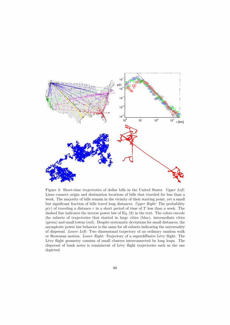
Figure 3: Short-time trajectories of dollar bills in the United States. Upper Left:Lines connect origin and destination locations of bills that traveled for less than aweek. The majority of bills remain in the vicinity of their starting point, yet a smallbut significant fraction of bills travel long distances. Upper Right: The probabilityp(r) of traveling a distance r in a short period of time of T less than a week. Thedashed line indicates the inverse power law of Eq. (8) in the text. The colors encodethe subsets of trajectories that started in large cities (blue), intermediate cities(green) and small towns (red). Despite systematic deviations for small distances, theasymptotic power law behavior is the same for all subsets indicating the universalityof dispersal. Lower Left: Two dimensional trajectory of an ordinary random walkor Brownian motion. Lower Right: Trajectory of a superdi"usive Levy flight. TheLevy flight geometry consists of small clusters interconnected by long leaps. Thedispersal of bank notes is reminiscent of Levy flight trajectories such as the onedepicted.

62

journeys of this distance in a short period of time. This quantity is shown in Fig. 3.This estimate was based on a dataset of 464,670 individual bills. On a range ofdistances between 10 and 3,500 km, this probability follows an inverse power law,i.e.

p(r) ( 1r1+µ

, (8)

with an exponent µ % 0.6. Despite the multitude of means of transportation in-volved, the underlying complexity of human travel behavior and the strong spatialheterogeneity of the United States, the probability follows this simple mathemati-cal law indicating that human mobility is governed by underlying universal rules.Moreover the specific functional form has important consequences. If one assumesthat individual bills perform a spatial random walk with an arbitrary probabilitydistribution p(r) for distances at every step one can ask: What is the typical dis-tance |X(t)| from the initial starting point as a function of time? For ordinaryrandom walks (Brownian motion) that are ubiquitous in the natural sciences, the

behavior of |X(t)| is determined by the standard deviation " =""r2# ! "r#2 of the

single steps and, irrespective of the particular shape of the distance distribution,scales according to the ‘square root law’, i.e. |X(t)| (

)t, a direct consequence of

the central limit theorem[17]. However, for a power law of the type observed in thedispersal of bank notes the variance diverges for exponents µ < 2 and the situa-tion is more complex. It implies that the dispersal of bank notes lacks a typicallength scale, is fractal and the trajectories of bills are reminiscent of a particularclass of random walks known as Levy flights[18, 19]. Levy flights, as opposed toordinary random walks, are anomalously di"usive, they exhibit a scaling relationthat depends on the exponent:

|X(t)| ( t1/µ. (9)

Because Levy flights are superdi"usive, they disperse faster than ordinary randomwalks, and their geometrical structure di"ers considerable from ordinary randomwalks, see Fig. 3. The discovery that the dispersal of bank notes and thereforehuman travel behavior lacks a scale and is related to Levy flights was a majorbreakthrough in understanding human mobility on global scales.

3 Statistical Properties and Scaling Laws in MultiScale Mobility Networks

Figure 4 illustrates a proxy network obtained from the flux of dollars in the UnitedStates, including all spatial scales. This network is defined by 3109 nodes (countiesin the United States excluding Alaska and Hawaii) connected by weights Wnm thatrepresent the flux rate of bills from county m to n in units of bills per day. Theentire network structure is thus encoded in the 3109 * 3109 flux matrix W. Aseach location has a well-defined geographical position, this multi-scale US tra!c

63

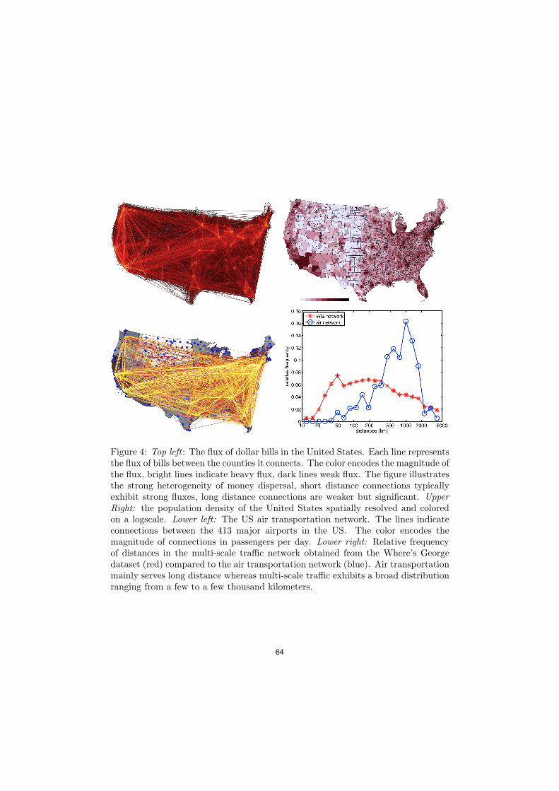
Figure 4: Top left : The flux of dollar bills in the United States. Each line representsthe flux of bills between the counties it connects. The color encodes the magnitude ofthe flux, bright lines indicate heavy flux, dark lines weak flux. The figure illustratesthe strong heterogeneity of money dispersal, short distance connections typicallyexhibit strong fluxes, long distance connections are weaker but significant. UpperRight: the population density of the United States spatially resolved and coloredon a logscale. Lower left: The US air transportation network. The lines indicateconnections between the 413 major airports in the US. The color encodes themagnitude of connections in passengers per day. Lower right: Relative frequencyof distances in the multi-scale tra!c network obtained from the Where’s Georgedataset (red) compared to the air transportation network (blue). Air transportationmainly serves long distance whereas multi-scale tra!c exhibits a broad distributionranging from a few to a few thousand kilometers.

64

Figure 5: Symmetry of the money circulation network. The figures depicts thecorrelation F in

n and F outn of flux of bill in and out and the in- and out degree kin

n

and koutn of a node n for all 3109 nodes in the network. The dashed lines represent

the linear relationships.

network can be visualized as a geographically embedded network as shown in thefigure. Qualitatively, one can see that prominent East coast – West coast fluxes existin the network. Yet the strongest connections are short to intermediate length scaleconnections, as opposed to the air transportation network that serves long distanceonly. Although every day 2.35 million passengers travel on the US air transportationnetwork, this represents only a small subset of the multi-scale tra!c network. Thehistogram in Fig. 4 illustrates these properties more quantitatively, comparing therelative frequency of distances in the multi-scale Where’s George network comparedto the air transportation network. Clearly, the majority of distances served by airtransportation peaks around 1000 km, whereas distances in the multi-scale networkare broadly distributed across a wide range from a few to a few thousand kilometers.

In order to understand human mobility on all spatial scales it is therefore essen-tial to include all means of transportation indirectly involved in the Where’s Georgemoney circulation network. The bill circulation network quantified by the flux ma-trix can give important insight into the statistical features of human mobility acrossthe United States. In order to quantify the statistical features of the network wewill concentrate on the flux of bills in and out of a node given by

F inn =

!

m

Wnm F outn =

!

m

Wmn, (10)

respectively. These flux measures are a direct proxy for the overall tra!c capacityof a node in the network. Furthermore we will investigate the in- and out degree of

65

a node defined according to

kinn =

!

m

Anm koutn =

!

m

Amn, (11)

where the elements Anm are entries of the adjacency matrix A. These elements areeither one or zero depending on whether nodes are connected or not. The degreeof a node quantifies the connectivity of a node, i.e. to how many other nodes agiven node is connected. A first important but expected feature of the multi-scalemobility network is its degree of symmetry. Figure 5 depicts the correlation of theflux of bills in and out of each node and a correlogram of the in- and out-degrees.These quantities exhibit a linear relationship subject to fluctuations,

F inn % F out

n kinn % kout

n , (12)

indicated by the dashed lines in the figure. Note also that the magnitude of the fluxvalues ranges over nearly four orders of magnitude, a first indication of the strongheterogeneity of the network.

Figure 6: Heterogeneity of multi-scale human mobility networks. Cumulative prob-ability distributions of the population size of the nodes (top left), the weight matrixelements Wnm (top right), the flux of bills Fn in and out of nodes (bottom left) andthe degree kn of the nodes (bottom right). The broadness of these distributions isa consequence of the strong heterogeneity of the network.

66

This high degree of heterogeneity is further illustrated by the cumulative distri-butions of the weights, the fluxes and the degrees of all the nodes in the networkas depicted in Fig. 6. All quantities are broadly distributed across a wide rangeof scales. Very similar broad distributions have been observed in studies of the airtransportation networks[7, 4, 14]. A very important issue in transportation the-ory is the development of a plausible evolutionary mechanism that can account forthe emergence of these distributions, a task that has not been accomplished so far.There is no plausible ‘theory’ for human tra!c networks as of today that predictsthe precise functional form of the distributions shown in Fig. 6.

Scaling Laws in the Topological Features of Multi-Scale Trans-portation Network

Figure 7: The functional dependence of influx F in (left) and in-degree kin (right) onthe population size P of a node. The flux of bills depends linearly on the populationsize (gray dashed line), whereas the degree exhibits a sublinear dependence (pinkdashed line).

In order to reveal additional structure in multi-scale human mobility networkswe investigated the functional relation of the quantities defined above, i.e.: Whatis the functional relation of fluxes and degrees with respect to the population sizeof a node? Figure 7 illustrates the statistical relationship between population sizeof a node and the flux of bills into a node. The dashed line in the figure representsa linear relationship with slope one, indicating that tra!c through a node growslinearly with the population size:

F (P ) ( P. (13)

Intuitively this is expected: the larger the population of a node the more tra!c flowsin and out of it. However, correlating the degree of a node against the population

67

size indicates a sublinear relationship,

k(P ) ( P !, (14)

with an exponent # % 0.7, contrasting the intuitive notion that the connectivity ofa node grows linearly with population size as well. From the scaling relations (13)and (14) we can determine an important property of multi-scale mobility networks.The typical strength of a connection is given by the ratio of flux and degree andone obtains heuristically

W ( P 1!!. (15)

This implies that larger counties are not only connected to a larger number of othercounties but also that the typical strength of every connection is stronger. Bothrelations are determined by the universal exponent # = 0.7 and these relations holdover nearly four orders of magnitude, a surprising regularity exhibited by the multi-scale mobility network. Again, no theory exists that can account for these scalingrelations and the value of the exponent.

4 Spatially Extended Epidemic Models

In summary, two prominent features of multiscale human mobility networks emergedin the analysis above: (1) Networks exhibit a strong heterogeneity, the distributionof weights, tra!c fluxes and population sizes of communities range over many ordersof magnitude. (2) Although the interaction magnitude in terms of tra!c intensitiesdecreases with distance, the observed power-laws indicate that long range inter-actions play a significant role in spatial disease dynamics. In the models to bediscussed below, we will introduce a class of spatially extended models in whichthe impact and interplay of both spatial heterogeneity as well as long range spatialinteractions can be investigated in a systematic fashion. It will also become clearthat another key issue in spatial disease dynamics is the translation of topologicalfeatures of transportation networks, i.e. the flux matrix W into dynamical entitiesthat generate the dispersal in space. At first glance, this may seem to be a straight-forward process. However, as we will see, this is a nontrivial task, and the behaviorof a spatially extended epidemic model depends sensitively on the precise choice oftranslating the topology of a transportation network into dynamics. To understandthis, we first review some of the paradigmatic models for disease dynamics in asingle population.

4.1 Disease Dynamics in a Single Population

One of the simplest models for an epidemic in a single population is the SIRmodel[20]. In this model a population of N individuals is classified according toinfectious state, i.e. a person can be susceptible (S) to the disease, infected (I) bythe disease, and recovered (R) from the disease. Recovered individuals are assumed

68

to have acquired immunity to the disease and can no longer be infected. Eachindividual in a population may undergo the transition

S + I + R (16)

during the time course of an infection. The dynamics of an epidemic is governed byonly two reactions:

S + I"!+ 2I, (17)

I#!+ R, (18)

a contact-initiated disease transmission and the recovery from disease, respectively.Models of this type are known as compartmental models, because a population isdivided into di"erent compartments defining the state of the system and reactionsbetween individuals of various compartments define the dynamics. A key premise inthe SIR model – and in fact most single population compartmental models – is themixing assumption. It means that (1) all individuals of a given class are identical intheir behavior and (2) independent of one another and that (3) reactions between agiven pair of individuals occurs with the same likelihood as a reaction of any otherpair.

The structure of compartmental models is very similar in nature to chemicalreactions, in fact one usually employs the mass-action principle to derive ordinarydi"erential equations for the dynamics of the number of susceptibles, infecteds andrecovereds: At any point t in time the probability that an infected individual re-covers in [t, t + #t] is assumed to be constant and proportional to #t. The changein infecteds and recovered is thus

#I = !#R % !$#t. (19)

The probability that an infected successfully transmits the disease to a susceptiblein #t is given by

P = #t* " * T * S

N, (20)

where " is the contact rate between individuals, T the transmission probability andS/N the probability that the contact is with a susceptible individual. This yields

!#S = #I % %S I

N#t (21)

where % = "T is the force of infection, i.e. the e"ective transmission rate. Forthe SIR-model this yields the following system of nonlinear ordinary di"erentialequations (ODEs):

&tS = !%S I

N,

&tI = %S I

N! $I,

&tR = $I. (22)69

We can define fractions s = S/N , j = I/N and r = R/N and noting that S(t) +I(t) + R(t) = N (i.e., the population size is conserved) we obtain the SIR model inits canonical form[21]:

&ts = !%sj,

&tj = %sj ! $j, (23)r = 1! s! j.

The key parameter in the SIR model is the basic reproduction number:

R0 =%

$=

Trecovery

Tcontacts,

the ratio of the force of infection and recovery rate. It is the average number ofsecondary infections caused by one infected individual during the time that indi-vidual is infected, on average. When R0 > 1, a population with an initially smallfraction of infecteds will be subject to an epidemic: a fast exponential increase anda subsequent decay of j(t), see Fig. 8. When R0 < 1 no epidemic occurs. The basicreproduction number is thus a threshold parameter.

Figure 8: Time evolution of the SIR model as defined by Eqs. (23). Parametersare $ = 1 and R0 = 4.5. Time course of the fraction of infecteds, susceptibles andrecovereds are shown in red, blue and green respectively. The initial condition wasj(0) = 0.01, s(0) = 1! j(0) and r(0) = 0.

70

The SIS model

In the SIS model the second reaction scheme (18) is replaced by I + S, infectedindividuals do not acquire immunity but rather recover from the disease to becomesusceptible again. This model lacks the R class and is governed by only one ODEfor the infecteds,

&tj = %j(1! j)! $j, (24)

where the conservation of individuals s = 1! j is assumed. For R0 = %/$ > 1 theSIS model evolves to a stable stationary state given by

js = 1! 1R0

,

in which a fraction js of the population is infected, the disease is endemic. The SISmodel is a useful system for investigating the impact of space on disease dynamicsand we will discuss the spatially extended SIS model in the next section.

4.2 Spatial Models

In the heart of all spatial models is the motivation to forsake the assumption of ho-mogeneous mixing of individuals and incorporate the fact that individuals belongingto di"erent populations exhibit di"erent interaction probabilities and that they aremobile in space. The conceptual tool underlying the development of spatial modelsis that of a metapopulation. A metapopulation is a set m = 1, ...,M of populationsof size Nn. The total number of individuals of the metapopulation is

N =M!

n=1

Nn. (25)

It is usually assumed that the dynamics in each population is governed by dynamicsthat adhere to homogeneous mixing but interaction of individuals between popula-tions are governed by additional laws. The most important of such interactions fordisease dynamics is the random exchange of individuals between populations. Themost straightforward generalization of the SIS model including metapopulations isgiven by:

Sn + In"!+ 2In

In#!+ Sn

Snwmn!!!+ Sm

Inwmn!!!+ Im (26)

In addition to the first two reactions, i.e. ordinary SIS dynamics in each populationn, susceptibles and infecteds can randomly move between population m and n, therate of which is governed by the probability rate wmn. The assumption in this

71

model is that individuals of all types randomly travel between populations in thesame fashion. The set of ODEs governing disease dynamics is then given by an setof 2M coupled ODEs:

&tSn = !%SnIn

Nn+ $In +

!

m"=n

[wnmSm ! wmnSn] ,

&tIn = %SnIn

Nn! $In +

!

m"=n

[wnmIm ! wmnIn] . (27)

The total rate of leaving a node n is given by#

m"=n wmn and the expected timean individual remains in a population n is

"Tn# =1#

m"=n wmn. (28)

Note that in the metapopulation system the number Nn(t) = Sn(t) + In(t) ofindividuals in each subpopulation is generally time-dependent, in fact adding theODEs pairwise we obtain

&tNn =!

m"=n

[wnmNm ! wmnNn] . (29)

In most models it is usually assumed that the system is equilibrated with respectto dispersal, i.e. Nn does not change over time and is therefore equal to the fixedpoint of Eq. (29), i.e.

Nn(t) = Nsn = Cn = const. (30)

In the following we will refer to the stationary population size of node n as thecapacity Cn. In equilibrium the flux of individuals from n to m balances that of mto n (detailed balance condition):

wnmCm = wmnCn. (31)

In this case the spatial SIS model (27) reduces to a set of M coupled ODEs for thefraction of infecteds in each population:

&tjn = %jn(1! jn)! $jn +!

m"=n

[wnmjm ! wmnjn] , (32)

with jn = In/Cn. The system defined by (32) is an example of an infectiousdisease dynamical system extended to the metapopulation level. A large class ofcontemporary models for spatial disease dynamics are related in structure to it[5, 22,15, 9]. One of the key di!culties in theoretical epidemiology are (1) the identificationof e"ective communities of populations that make up a metapopulation and (2) thequantitative assessment of travelling rates wnm between these populations. Notethat the introduction of populations n making up the metapopulation did not specify

72

spatial locations. In the dynamical system (32), the relation between communitiesis solely defined by the dynamical coupling 'nm. In most models, however, allcommunities are typically embedded in space such that each population n has a welldefined geographical location xn. One can then use the geographical information tomake and test assumptions on how the exchange rates wnm depend on geography.One of the most popular assumptions in this context is that the flux of individualsbetween two communities depends on their size and their distance. The total fluxof individuals in equilibrium from community m to n and vice versa is given by theleft and the right hand side of the detailed balance condition (31), respectively. Inthe majority of models it is assumed that the flux Fnm increases with the capacities(i.e. the stationary size of the populations) Cm and Cn and decreases monotonicallywith the geographic distance between them, i.e.

Fnm = '0 (CmCn)! G (|xn ! xm|) = Fmn, (33)

with 0 , # , 1. The function G takes care of the dependence on distance. De-pending on the type of metapopulation and dynamical context, this kernel canbe exponential, Gaussian or show an algebraic decay with x. Using the relationFnm = wnmCm between absolute flux and probability rates in equilibrium, Eq. (33)implies for the hopping rate

wnm = w0C!n *G (|xn ! xm|)* C!!1

m . (34)

Inserted into the rate equation (29) one can check that Cn is the equilibrium com-munity size. In epidemiological contexts, spatial communities often reflect cities,towns and villages. The specific choice of G(x) put forth by Eq. (8) is the power-lawdecay

G(x) ( x!1!µ. (35)

Inserted into Eqs. (33) and (34) gives

'nm = '0C!

n * C!!1m

|xn ! xm|D+µ , (36)

where D = 2 is the spatial dimension. The parameter # quantifies the impact oforigin and destination in the travelling event m + n:

• When # = 1 we have

wnm - Cn and Fnm - CnCm. (37)

This implies that the rate is independent of properties of the origin and theflux is proportional to the size of both communities.

• When # = 0 we have

wnm - 1Cm

and Fnm - 1, (38)

73

i.e. the rate of traveling to destination n is independent of properties of thedestination and the flux is independent of community sizes of both places.

• An interesting system is the symmetric case when # = 1/2. This implies that

wnm -$

Cn/Cm and Fnm -$

CnCm. (39)

In this situation, the rate wnm is independent of scaling the entire metapopu-lation size uniformly by some factor and the flux is the geometric mean of thecommunity sizes of origin and destination. That implies for example: Whenwe scale the entire population size by Cn + 2Cn this scales the flux by afactor of two as well.

4.3 Continuity Limit and Fractional Transport

With the definition of the rate according to (36) the dispersal of individuals is givenby

&tNn = w0

!

m"=m

%C!

nC!!1m

|xn ! xm|2+µ Nm !C!

mC!!1n

|xm ! xn|2+µ Nn

&

with µ > 0. Useful insight into the properties of this master equation can be gainedby performing a continuity limit. Letting xn be points on a grid of microscopicareas #A and Nn(t) = n(xn, t)#A, Cn = c(xn)#A the above equation becomes

&tn(x, t) = w0 lim!A#0

ˆ

y/$!Ady

c!(x)c!!1(y)n(y, t)! c!(y)c!!1(x)n(x, t)|x! y|2+µ . (40)

The integral is over all points outside of an area centered at x. One has to be carefulcarrying out this limit, because of the divergent denominator. In fact, originallythe rate m + n was only defined for interacting communities n $= m and it ismeaningless for n = m. One can, however, carry out the limit #A + 0 andinterpret the integral as a Cauchy integral. The limit of the rhs. of (40) thendepends sensitively on the value of the exponent µ. For µ > 2 one obtains[23, 24]

&tn = D0

'c!#c!!1n! c!!1n#n!

(, (41)

with n = n(x, t) and c = c(x) and # is the second spatial derivative. This impliesthat when the exponent µ exceeds the critical value µc = 2 the process becomesa di"usion process in the limit above. However, this di"usion process evolves in aheterogeneous environment determined by the function c(x).

If µ < 2, as for example observed in the dispersal of bank notes (in that caseµ % 0.6), the limit yields

&tn = D0

)c!#µ/2c!!1n! c!!1n#µ/2n!

*(42)

74

where the operator #µ/2 is known as the fractional Laplacian, a non-local singularoperator defined by

(#µ/2f)(x) = Cµ

ˆ

dyf(y)! f(x)|x! y|D+µ (43)

where Cµ is a constant and D the spatial dimension[25, 26]. The reason why #µ/2 isreferred to as a fractional derivative is that in Fourier space it exhibits a particularlysimple form, a multiplication by !|k|µ. Equations of the type (42) are known asfractional di"usion equations and have been employed in a number of physical,biological and chemical systems[27, 28, 29, 30], ranging from anomalous di"usionof protein motion on folded polymers to human eye-movements[31, 25, 26]. Thederivation above relates dispersal of individuals in metapopulations to fractionaldi"usion equations for the first time, an approach that may well prove to be valuablein the future.

4.4 Limiting Cases

Before reinserting the dispersal component into the original spatial SIS model, itis worthwhile considering known marginal cases of the general fractional di"usionequation (42). For example when µ = 2 and c(x) = 1 the dynamics equation reducesto

&tn = D0#n, (44)

i.e. ordinary di"usion in a homogeneous environment. When µ = 2 but c(x) is avariable function of position, i.e. Eq. (42) is the same as Eq. (41), the dispersal isgoverned by a Fokker-Planck equation

&tn = !.F n +12#D n, (45)

which is equivalent to (41), and force and di"usion coe!cients F = F (x) andD = D(x), respectively, are related to the heterogeneity function c(x). This relationdepends, of course, on the value of the parameter #. For example, when the systemis origin-driven, i.e. when # = 0, Eq. (41) reduces to

&tn = D0#n/c, (46)

a Fokker-Planck equation with a space dependent di"usion coe!cient

D(x) =D0

c(x)(47)

that is inversely proportional to the stationary population density c(x). This meansthat in this system di"usion is high in regions where the population is small and viceversa. In the destination driven system # = 1, we obtain a Fokker-Planck equationwith

D(x) = 2D0c(x) and F (x) = 2D0.c(x). (48)75

Here, di"usion increases with population density, but more importantly a nonzerodrift towards regions with higher population density is introduced. When µ = 1/2,i.e. the impact of origin and destination are the same, the di"usion coe!cient isconstant and the force term is given by

F (x) = D0. log c(x). (49)

One can see that only in this situation the dynamics does not change when thepopulation density c(x) is scaled uniformly by some factor. In this case ! log c(x)can be considered a potential V (x) of the system, with minima in densely populatedareas and maxima in weakly populated ones.

The most interesting case and certainly the one closest to reality is the generalcase, when the dynamical system is fractional di"usive and spatially heterogeneous.The combination of the rhs. of (42) with the spatial SIS model of Eq. (32) gives thespatially extended fractional SIS model,

&tj = %j(1! j)! $j + D0c!!1

)#µ/2c!j ! j#µ/2c!

*. (50)

The spatial SIR model or related systems that di"er in the local dynamics can bederived analogously, for instance the spatial SIR model is given by

&ts = !%js + D0c!!1

)#µ/2c!s! s#µ/2c!

*, (51)

&tj = %js! $j + D0c!!1

)#µ/2c!j ! j#µ/2c!

*.

The key question is: What are the general properties of solutions to these reactionfractional di"usion equations? How do their solutions depend on the parameters0 , # , 1 and 0 < µ , 2 ? And what are approximate choices for these parametersfor real epidemics?

To address the first question, solutions of three variants of the spatial SIR modelare depicted in Fig. 9. One system is spatially homogeneous and dispersal is ordi-nary di"usion. The solution exhibits traveling wavefronts that propagate at constantspeeds, a fact known for similar systems such as the Fisher equation. In fact, a spa-tially homogeneous SIR variant was employed to estimate the speed of propagationof the black death in Europe in the 14th century. The second simulation is a systemwith some degree of spatial heterogeneity, i.e. c(x) is variable but µ = 2. As in thespatial homogeneous system, solutions to the spatial SIR model still exhibit well-defined traveling wavefronts that exhibit some irregularity imposed by the spatialheterogeneity. However, the key feature of a wavefront propagating with a constantspeed remains unchanged.

If however, one introduces non-local dispersal by choosing a value µ < 2, theoverall statistical features of the spreading pattern changes drastically. Instead ofa well shaped wavefront the pattern exhibits localized islands in the time course ofthe epidemic. This behavior is a direct consequence of the interplay of the spatial

76

Figure 9: Snapshots of a two-dimensional spatially extended SIR model. Top: Aspatially homogeneous system with c(x) = const and ordinary di"usion in space.This system exhibits a propagating front at constant speed. Center : The same asabove but with spatial heterogeneity. The heterogeneity induces randomness in theshape of the wavefront but produces no qualitatively di"erent patterns. Bottom:The fractional SIR model with heterogeneity. The combination of scale-free di"usionand heterogeneity introduces a novel type of spatiotemporal pattern with fractalproperties.

77

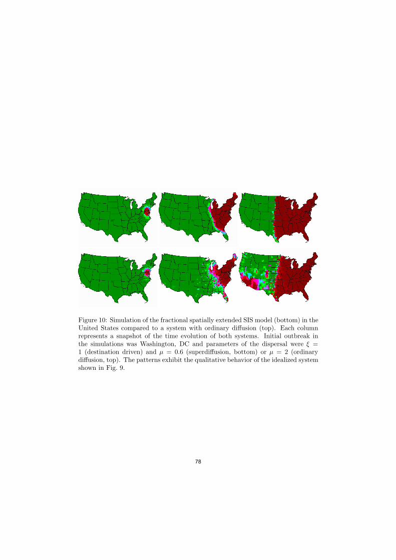
Figure 10: Simulation of the fractional spatially extended SIS model (bottom) in theUnited States compared to a system with ordinary di"usion (top). Each columnrepresents a snapshot of the time evolution of both systems. Initial outbreak inthe simulations was Washington, DC and parameters of the dispersal were # =1 (destination driven) and µ = 0.6 (superdi"usion, bottom) or µ = 2 (ordinarydi"usion, top). The patterns exhibit the qualitative behavior of the idealized systemshown in Fig. 9.

78

heterogeneity and the non-local superdi"usive nature of dispersal incorporated inthe fractional SIR model (51).

The last questions can be answered by a comparison to the empirical resultspresented above. The fact that the flux of dollar bills into nodes is proportionalto the population size suggests that human dispersal is destination driven, see forexample Eq. (37) and that # = 1. The power-law in the short time dispersalprobability for the distance, i.e. p(r) in Eq. (8) implies that µ % 0.6. With theseparameters, and the equilibrium distribution of individuals in a large geographicarea, we can investigate the spreading pattern in a real geographic context. Resultsare shown in Fig. 10 for a fractional SIS model with parameters µ = µh % 0.6 inthe United States for an initial outbreak in Washington, DC. For c(x) we chosethe population density of the counties in the United States. In comparison to asystem with only local dispersal, the fractional SIS systems shows a pattern similarin structure to the idealized system of a square grid (i.e. Fig. 9). For instance,well before the bulk of the epidemic reaches the Midwest, the disease has alreadyalmost reached is maximum in urban areas on the West-Coast. Despite its structuralsimplicity and the crude assumptions made on the course of deriving the fractionalSIS model, these spreading patterns are strikingly similar to recently publishedlarge scale agent based simulation studies on the most likely spread of new humaninfluenza H5N1 subtype in the United States.

Although these results are promising, from a theoretical point of view little isknown about the general properties of fractional and heterogeneous reaction di"u-sion equations such as (50) and (51). This is primarily due to the fact that theseequations are di!cult to solve numerically and the analytical tools for investiga-tion are currently underdeveloped. The richness of possible applications of thisapproach, not only in spatial epidemiology, however, leads us to believe that inthe near future novel and interesting properties of fractional di"usion systems inheterogeneous environments will be discovered and will find their identification innatural systems.

Acknowledgements The authors would like to thank Rafael Brune and ChristianThiemann for their help in improving the manuscript, and Daniel Grady and OliviaWoolley for useful comments.

References

[1] YC Xia, ON Bjornstad, and BT Grenfell. Measles metapopulation dynamics: Agravity model for epidemiological coupling and dynamics. Am Nat, 164(2):267–281, Jan 2004.

[2] http://www.who.int/csr/disease/swineflu.

[3] http://rocs.northwestern.edu/projects/swine flu.

79

[4] L Dall’Asta, A Barrat, M Barthelemy, and A Vespignani. Vulnerability ofweighted networks. J Stat Mech-Theory E, page P04006, Jan 2006.

[5] V Colizza, R Pastor-Satorras, and A Vespignani. Reaction-di"usion processesand metapopulation models in heterogeneous networks. Nat Phys, 3(4):276–282, Jan 2007.

[6] V Colizza, A Barrat, M Barthelemy, and A Vespignani. The role of the airlinetransportation network in the prediction and predictability of global epidemics.P Natl Acad Sci Usa, 103(7):2015–2020, Jan 2006.

[7] A Barrat, M Barthelemy, and A Vespignani. The e"ects of spatial constraintson the evolution of weighted complex networks. J Stat Mech-Theory E, pageP05003, Jan 2005.

[8] JV Noble. Geographic and temporal development of plagues. Nature,250(5469):726–728, Jan 1974.

[9] BT Grenfell, ON Bjornstad, and J Kappey. Travelling waves and spatial hier-archies in measles epidemics. Nature, 414(6865):716–723, Jan 2001.

[10] BT Grenfell, ON Bjornstad, and BF Finkenstadt. Dynamics of measles epi-demics: Scaling noise, determinism, and predictability with the tsir model.Ecol Monogr, 72(2):185–202, Jan 2002.

[11] NM Ferguson, DAT Cummings, S Cauchemez, C Fraser, S Riley, A Meeyai,S Iamsirithaworn, and DS Burke. Strategies for containing an emerging in-fluenza pandemic in southeast asia. Nature, 437(7056):209–214, Jan 2005.

[12] NM Ferguson, DAT Cummings, C Fraser, JC Cajka, PC Cooley, and DS Burke.Strategies for mitigating an influenza pandemic. Nature, 442(7101):448–452,Jan 2006.

[13] MC Gonzalez, CA Hidalgo, and AL Barabasi. Understanding individual humanmobility patterns. Nature, 453(7196):779–782, Jan 2008.

[14] R Guimera and LAN Amaral. Modeling the world-wide airport network. EurPhys J B, 38(2):381–385, Jan 2004.

[15] L Hufnagel, D Brockmann, and T Geisel. Forecast and control of epidemics ina globalized world. P Natl Acad Sci Usa, 101(42):15124–15129, Jan 2004.

[16] D Brockmann, L Hufnagel, and T Geisel. The scaling laws of human travel.Nature, 439(7075):462–465, Jan 2006.

[17] CW Gardiner. Handbook of Stochastic Methods. Springer Verlag, Berlin, 1985.

[18] R Metzler and J Klafter. The random walks guide to anomalous di"usion: Afractional dynamics approach. Phys. Rep., 339:1–77, 2000.

80

[19] MF Shlesinger, GM Zaslavsky, and U Frisch, editors. Levy Flights and RelatedTopics in Physics, Lecture Notes in Physics, Berlin, 1995. Springer Verlag.

[20] RM May and RM Anderson. Population biology of infectious-diseases .2. Na-ture, 280(5722):455–461, Jan 1979.

[21] WO Kermack and AG McKendrick. Contributions to the mathematical the-ory of epidemics ii - the problem of endemicity. P R Soc Lond A-Conta,138(834):55–83, Jan 1932.

[22] V Colizza and A Vespignani. Epidemic modeling in metapopulation systemswith heterogeneous coupling pattern: Theory and simulations. J Theor Biol,251(3):450–467, Jan 2008.

[23] VV Belik and D Brockmann. Accelerating random walks by disorder. New JPhys, 9:54, Jan 2007.

[24] D Brockmann and IM Sokolov. Levy flights in external force fields: Frommodels to equations. Chem. Phys., 284:409–421, 2002.

[25] D Brockmann and T Geisel. Particle dispersion on rapidly folding randomhetero-polymers. Phys. Rev. Lett., 91:048303, 2003.

[26] Dirk Brockmann and Theo Geisel. Levy flights in inhomogeneous media. Phys.Rev. Lett., 90(17):170601, 2003.

[27] E Barkai, R Metzler, and J Klafter. From continuous time random walks tothe fractional Fokker-Planck equation. Phys. Rev. E, 61(1):132–138, 2000.

[28] E Barkai. Fractional Fokker-Planck equation, solution, and application. Phys.Rev. E, 63:46118, 2001.

[29] AI Saichev and GM Zaslavsky. Fractional kinetic equations: solutions andapplications. Chaos, 7(4):753–764, Jan 1997.

[30] R Metzler and J Klafter. Boundary value problems for fractional di"usionequations. Physica A, 278:107–125, 2000.

[31] D Brockmann and T Geisel. The ecology of gaze shifts. Neurocomputing,32-33:643–650, 2000.

81