How to Quantify Culture

Outline of Today’s Talk

Several Main Parts:1. What is culture?2. Why quantify culture?3. How to quantify culture?4. Three ExamplesThe full R code template for these analyses is available by emailing me at: fosse.ethan@gmail.com

What is Culture?

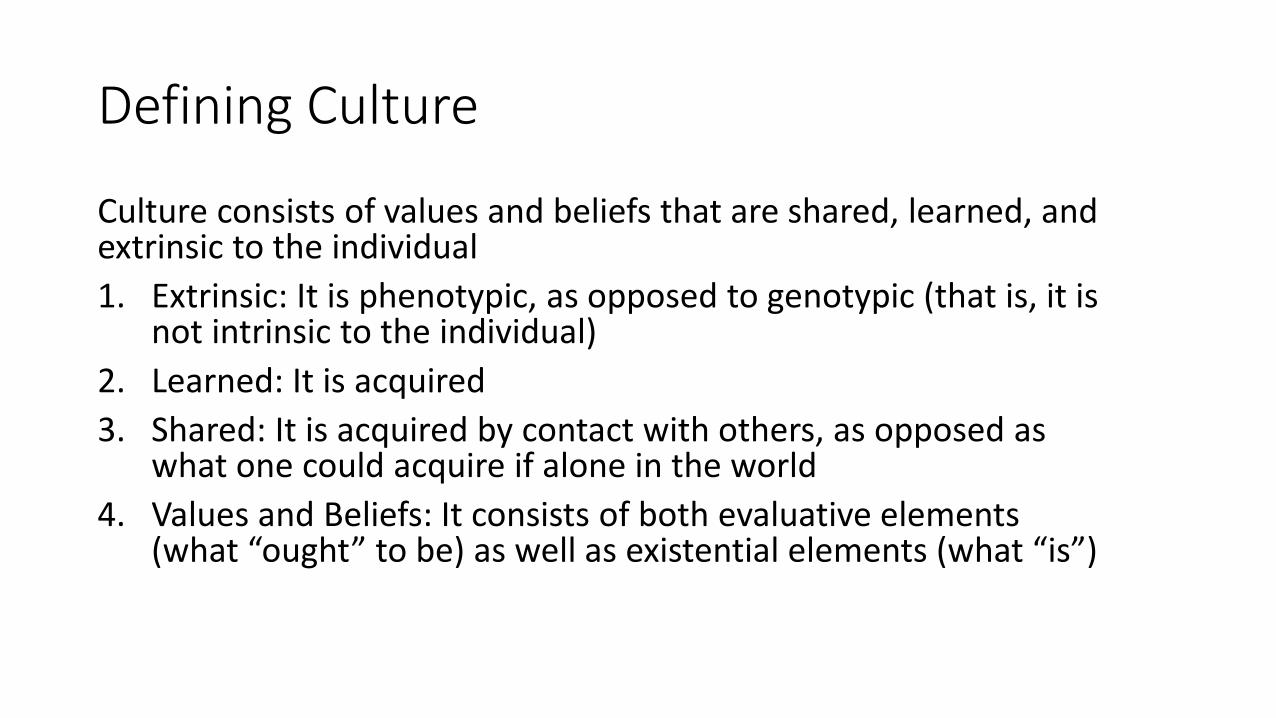
Defining Culture

Culture consists of values and beliefs that are shared, learned, and extrinsic to the individual1. Extrinsic: It is phenotypic, as opposed to genotypic (that is, it is

not intrinsic to the individual)2. Learned: It is acquired3. Shared: It is acquired by contact with others, as opposed as

what one could acquire if alone in the world4. Values and Beliefs: It consists of both evaluative elements

(what “ought” to be) as well as existential elements (what “is”)

Early Efforts at Quantifying Culture

• Emile Durkheim (1890)• Attempted to claim that suicide is caused by different cultural

contexts• In particular, he thought that suicide rates were higher in areas with

greater cultural changes (causing a lack of “anomie”)• Used population changes as a proxy for cultural changes• Had no direct access to data on people’s beliefs and values

Early Efforts at Quantifying Culture

• Max Weber (1897): • Attempted to measure people’s relationship between their values and

occupation• 27-item survey• Admitted the problems with his survey

• 1911: “I agree that (these data) have no value for the question: why have these people really chosen their occupation? Possibly the answers are quite useless. I consider it possible, however, that they are worthwhile under another aspect; what do people answer to such an-if you please-stupid question? (Laughter.) Sometimes stupid questions provide quite val-uable answers. (Laugher.)”

Example: Google Books Project

For more, go to: https://books.google.com/ngrams

The “Digital Humanities”

Two flavors of “Digital Humanities”:1. Using statistical methods to

digitize books and improve library access

2. Using statistics to understand how people use language in various ways

Example: World Values Survey

• Based on work of Ronald Inglehart

• Uses cross-national surveys to examine people’s values and beliefs

• Cluster analyses of countries suggest cultural groupings

Example: “Cliometrics” and Quantifying History

• Cliometrics: Using statistics to better understand history

• Example: Why Nations Fail by Daron Acemoglu and James A. Robison

• Colonialism has a negative long-term effect if it’s merely extracting local resources

Many Other Applications

The applications are endless: sociology, anthropology (including cultural anthropology), political science, psychology, and so forth!

Why Quantify Culture?

Reason 1: Data Deluge

(1) Exponential growth and availability of all sorts of data (“Internet of Things”)

(2) Increasing in volume, velocity, variety (veracity?)(2) Huge gap between exponential growth of data and number of people who can analyze these dataBottom line: We have more data than people to analyze them!

The World Needs You!

At no other time do we more urgently need careful data analysts and thinkers such as yourself to find those hidden facts and patterns that will change our world!

The Amount of Data is Growing Exponentially

Reason 2: Semantic Web

Bottom line: We increasingly have the kind of data that is cultural

Reason 3: Moravec’s Paradox

• AI researcher Hans Moravec observed in the 1980s that high-level reasoning requires very little computation while low-level reasoning is computationally difficult

• Examples: Deep Blue defeats chess, Watson beats Jeopardy• Easier to reverse-engineer mathematics, games, logic, statistics than it is

intuition, emotion, perception• The traditional practitioners of cultural analysis (historians,

anthropologists, qualitative market researchers) have the skill sets that are among the most difficult to automate!

Bottom line: Need for analysts who can “tell stories” or “give meaning”• This is why data analysis is not equivalent to mathematics

Reason 4: Data Science

(1) Huge increase in popularity in part because data science is modular, cross-disciplinary

(2) Advances in computation have allowed the processing of large amounts of data, especially text data(3) Easier now than in previous decades to learn tools of data science due to growth of online education and open-source scienceBottom line: Data science is growing in popularity and can provide the tools to analyze cultural phenomena.

An Aside: What is “Data Science”?

• Data science is a recently coined term from the 1970s• 1988: the statistician C.F. Jeff Wu elaborated on the phrase in a talk

titled “Statistics = Data Science?”• Argued that statisticians should rebrand themselves as “data

scientists” since spend most of their time manipulating and experimenting with data

• Until recently, data scientists have tended to focus more on cleaning datasets and programming

• My own view: “data science” = “applied statistics”

Data Science Venn DiagramR is a programmingLanguage!

Statistical problems and concepts!

From economics, sociology, finance, etc., or your own life experience!

Statistics as “Data Science”

• Statistics has been around for a relatively long time• “Data Science” is a new buzzword reflecting the huge increase in data

over the past several decades• No clear-cut definition• My own view: “data science” can be understood as “applied statistics”• Not just theory, but practical application is important!

How to Quantify Culture?

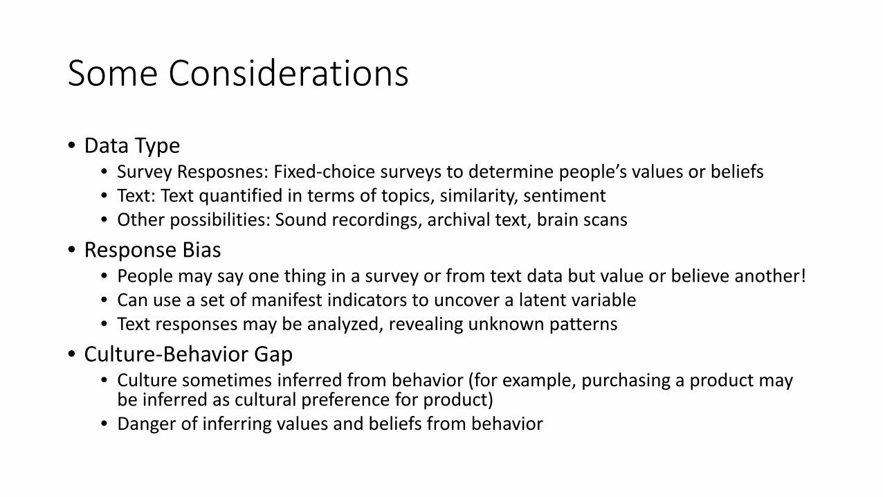
Some Considerations

• Data Type• Survey Resposnes: Fixed-choice surveys to determine people’s values or beliefs• Text: Text quantified in terms of topics, similarity, sentiment• Other possibilities: Sound recordings, archival text, brain scans

• Response Bias• People may say one thing in a survey or from text data but value or believe another!• Can use a set of manifest indicators to uncover a latent variable• Text responses may be analyzed, revealing unknown patterns

• Culture-Behavior Gap• Culture sometimes inferred from behavior (for example, purchasing a product may

be inferred as cultural preference for product)• Danger of inferring values and beliefs from behavior

Tips for Quantifying Culture

Basic requirements for the quantification of culture:1. Knowledge of the phenomena studied2. Access to cultural data (for example, text or survey responses)3. Facility with clustering techniques and statistical models4. Use of one or more statistical programming languages

• Why R?• These are not mutually exclusive!

Statistical Programming Languages

• Excel: popular among Wall Street types and business school grads (has limited programming functionality)

• MATLAB: often used by neuroscientists and engineers• SPSS: widely used by psychologists but has limited functionality• SAS: popular among biologists and biostatisticians• Python: popular among computer scientists; somewhat limited

statistics functionality but improving• Stata: popular among economists and financial analysts• R: used by statisticians and cool people; often used with RStudio

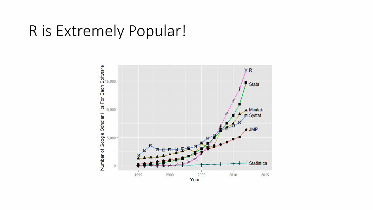
R is Extremely Popular!

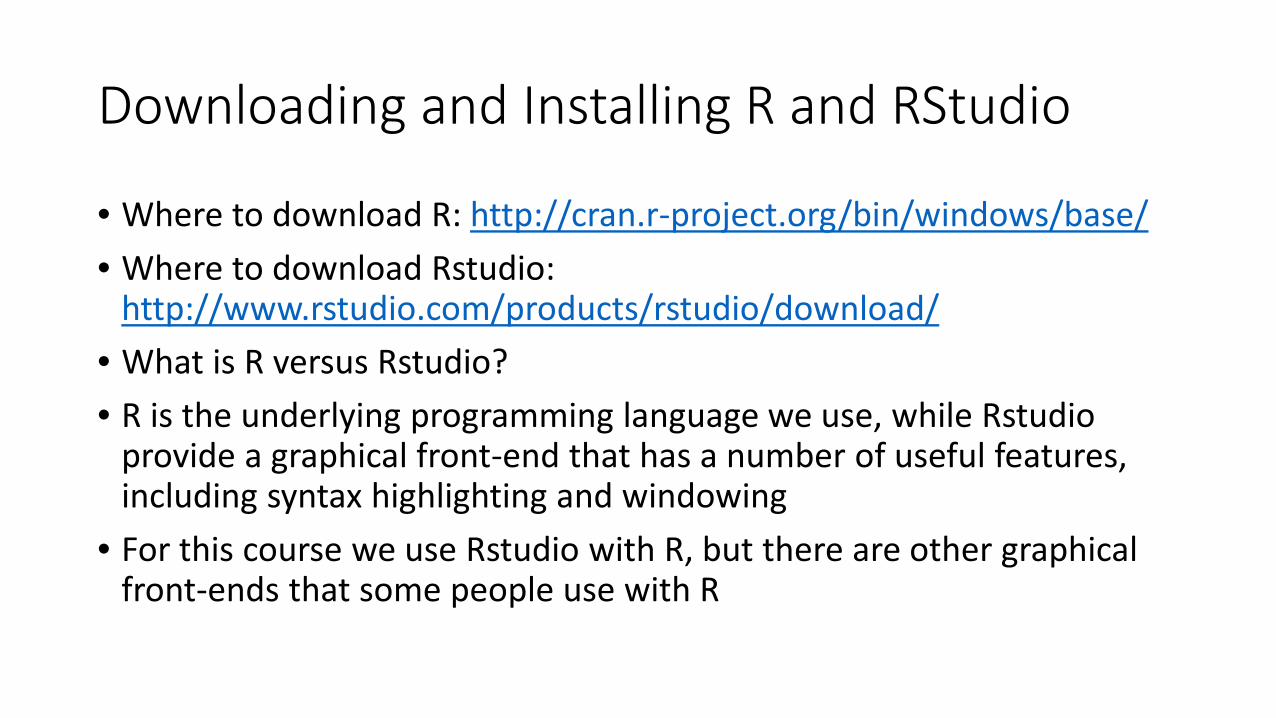
Downloading and Installing R and RStudio

• Where to download R: http://cran.r-project.org/bin/windows/base/• Where to download Rstudio:

http://www.rstudio.com/products/rstudio/download/• What is R versus Rstudio?• R is the underlying programming language we use, while Rstudio

provide a graphical front-end that has a number of useful features, including syntax highlighting and windowing

• For this course we use Rstudio with R, but there are other graphical front-ends that some people use with R

Things to Remember About R

• Unlike other programs (such as SPSS, Stata, or Excel), R can have many objects in the workspace

• Every object in R has a type (called a “class”). Always ask yourself: What kind of thing is this?

• There are many, many different ways to do something in R• The best way to learn R is to use it everyday

Three Main Types of R Files

• R scripts (ending in “.R”)• R markdown (ending in “.Rmd”)• R data (ending in “.Rdata”)• There are other files, but if you’re starting out these are the main files

with which you’ll want to become familiar

Example 1Cultural Consequences of the Great Recession

Cleaning Up Data# creating scales of main trust variables# note: levels from 1 (distrust) to 11 (trust)ess$People <-scale(as.numeric(ess$ppltrst))ess$Parliament <-scale(as.numeric(ess$trstprl))ess$Law <- scale(as.numeric(ess$trstlgl))ess$Police <-scale(as.numeric(ess$trstplc))ess$Politicians <-scale(as.numeric(ess$trstplt))ess$EU <- scale(as.numeric(ess$trstep))ess$UN <- scale(as.numeric(ess$trstun))ess$Parties <-scale(as.numeric(ess$trstprt))

# year variableess$year <- as.integer(ess$interview_year)hist(ess$year)

Correlations Among Trust Variables

df <- subset(ess, select=c(People:Parties))df.num <-as.data.frame(sapply(df, as.numeric)) rho <- cor(df.num, use="pairwise.complete.obs")print(rho)

# graphing correlation plotcor.plot(rho, numbers=TRUE)

Item-Based Clustering of Trust Variables# item-based clusterng of trust itemsic <- iclust(rho, beta=3, beta.size=1, beta.min=0.75, alpha=3, alpha.size=1, plot=FALSE) print(ic)# graphing iclust resultsiclust.diagram(ic, main="Item-based hierarchical clustering", short=FALSE, digits=1,

marg=c(0.1,0.1,2.5,0.1), colors=c("black", "blue"), e.size=1.4, cex=0.7, cluster.names=c("Political","Judicial","International","Governmental","C5","C6","C7"))

Creating Composite Scales

Composite Scales from Item-based Hierarchical Clustering Analysis

Cluster Items Mean Median Std. Dev. Cronbach's Alpha

V1 People 0 0.044 1 NULL

C3 c("EU", "UN") -0.001 0.082 0.931 0.82

C4c("Parliament", "Politicians", "Parties")

0.011 0.028 0.921 0.91

C2 c("Law", "Police") 0 0.057 0.917 0.8

Note: This table summarizes the composite scales created from an item-based hierarchical cluster analysis. The mean, median, and standard deviation for each scale is presented, as well as Cronbach's alpha.

Overall Trends from 2002-2013# overall trends: people.scale

df.sub <- na.omit(subset(df, select=c("year","country","people.scale")))

m <- lm(people.scale ~ 1 + bs(year, df=3), data=df)

summary(m)

# graphing findings

plot(allEffects(m), rug=FALSE, main="Trust in Other People", ylab="Standardized Scale", xlab="Year")

Other Trends from 2002-2013

Contextual Variation in Trust

Example 2Cultural Definition of Generations

Cleaning Up the Data# creating age variable (age)

gnex$age <- recode(gnex$age, c("99=NA"))

# creating cohort variable

gnex$cohort <- 2006 - gnex$age

# gens variable

# Millennials: 1980 to 2014; generation X: 1965 to 1979; baby boomers: 1946 to 1964

# silent generation: 1925 to 1945; greatest generation: 1901 to 1924 (or earlier)

gnex$gens <- cut(gnex$cohort, breaks=c(1894,1924,1945,1964,1979,2014),

labels = c("Greatest","Silent","Boomers","Gen X","Millennials"), na.rm=TRUE)

table(gnex$gens)

df <- gnex[ , c("gens","cohort","mygen","pargen","myprobs")]

# table for millennialsdf.sub <- as.data.frame(df[which(df$gens=="Millennials"), ])

Text Responses: Millennials

gens cohort mygen pargen myprobsMillennials 1985 lazy old good jobMillennials 1980 CAREFREE OLD billsMillennials 1985 TALL PEOPLE BIG BONED PEOPLE BEING A SINGLE

MOMMillennials 1983 lack of caring hard workingMillennials 1981 in touch conservativeMillennials 1987 FREEDOM HARD WORKERS GOOD GRADESMillennials 1982 in trouble Job securityMillennials 1982 Great Interesting Your ChildrenMillennials 1982 New Old Folks The price of gasMillennials 1987 bad lovely moneyMillennials 1983 drug their children's future educationMillennials 1982 new breed old timers

Text Responses: Gen X

gens cohort mygen pargen myprobsGen X 1968 HARD WORKING FINACIALGen X 1972 screwed wholesome dont have enough moneyGen X 1970 looking for a cause/lost sd character sd financesGen X 1973 pioneers hippys moneyGen X 1965 determined financesGen X 1970 fast paced moneyGen X 1967 NEW LIFE JOBS WORKERSGen X 1970 GENERATION X PACKRATSGen X 1973 in debt retired cost of livingGen X 1974 CIVIL CHANGE 49ERS RUSH FINDING LOVEGen X 1966 CREATIVE BABTBOONERSGen X 1965 lost almost done raising my kids

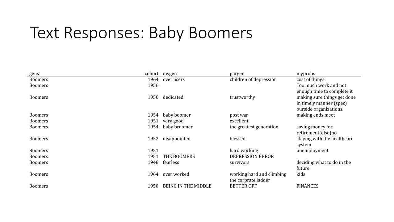
Text Responses: Baby Boomers

gens cohort mygen pargen myprobsBoomers 1964 over users children of depression cost of thingsBoomers 1956 Too much work and not

enough time to complete itBoomers 1950 dedicated trustworthy making sure things get done

in timely manner (spec) ourside organizations.

Boomers 1954 baby boomer post war making ends meetBoomers 1951 very good excellentBoomers 1954 baby broomer the greatest generation saving money for

retirement(else)noBoomers 1952 disappointed blessed staying with the healthcare

systemBoomers 1951 hard working unemploymentBoomers 1951 THE BOOMERS DEPRESSION ERRORBoomers 1948 fearless survivors deciding what to do in the

futureBoomers 1964 over worked working hard and climbing

the corprate ladderkids

Boomers 1950 BEING IN THE MIDDLE BETTER OFF FINANCES

Topic Proportions Overall

Expected Proportion of Topic by Cohort

Example 3Generational Trends in Religious and Political Views

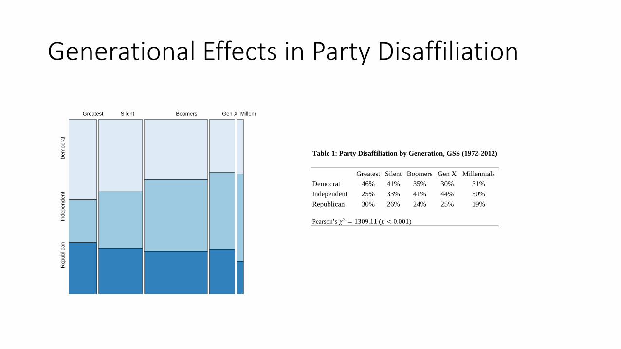
Generational Effects in Party Disaffiliation

Greatest

Rep

ublic

anIn

depe

nden

tD

emoc

rat

Silent Boomers Gen X Millenn

Table 1: Party Disaffiliation by Generation, GSS (1972-2012)

Greatest Silent Boomers Gen X Millennials Democrat 46% 41% 35% 30% 31% Independent 25% 33% 41% 44% 50% Republican 30% 26% 24% 25% 19%

Pearson’s 𝜒𝜒2 = 1309.11 (𝑝𝑝 < 0.001)

Generational Effects on Religious Disaffiliation

gens

g

Greatest

NoneOt

her

Cath

olic

Prot

esta

nt

Silent Boomers Gen X Millenn

Table 4: Religious Disaffiliation by Generation, Millennial Value Survey (2010)

Greatest Silent Boomers Gen X Millennials Protestant 50% 57% 49% 38% 31% Catholic 25% 21% 22% 22% 20% Mormon 4% 2% 2% 2% 2% Other Christian 4% 6% 7% 11% 14% Jewish 4% 3% 3% 1% 1% Muslim <1% <1% <1% 1% 2% Eastern Religion <1% <1% 1% 2% 1% Atheist or Agnostic <1% 2% 4% 4% 5% Something Else 11% 4% 3% 4% 6% Nothing 4% 4% 10% 16% 17% Pearson’s 𝜒𝜒2 = 48.19 (𝑝𝑝 < 0.001)

Multilevel Models of Generational Effects

0.2

0.3

0.4

GreatestSilent Boomer Gen X MillennialGeneration

Outco

me

0.2

0.3

0.4

1900 1925 1950 1975Cohort

Outco

me

0.30

0.35

0.40

0.45

25 50 75Age

Outco

me

0.325

0.350

0.375

0.400

0.425

1970 1980 1990 2000 2010Year

Outco

me

0.0

0.1

0.2

0.3

0.4

0.5

GreatestSilent Boomer Gen X MillennialGeneration

Outco

me

0.0

0.1

0.2

0.3

0.4

0.5

1900 1925 1950 1975Cohort

Outco

me

0.10

0.15

0.20

0.25

25 50 75Age

Outco

me

0.08

0.09

0.10

0.11

1970 1980 1990 2000 2010Year

Outco

me

Party Disaffiliation Religious Disaffiliation

To Recap

• Culture can be quantified through survey responses and text data• Clustering analyses embody the core concept beyond culture• Examining variation across clusters also crucial• The analysis of culture is nothing new!• If you want the R code underlying these analyses, please email me at:

fosse.ethan@gmail.com

End of PresentationBoston Data Festival