how to carry out assembly line–cell conversion? a

International Journal of Production ResearchVol. 50, No. 18, 15 September 2012, 5259–5280

How to carry out assembly line–cell conversion? A discussion based on factor analysis of

system performance improvements

Yang Yua, Jun Gonga, Jiafu Tanga, Yong Yinb and Ikou Kakuc*

aInstitute of Systems Engineering, State Key Laboratory of Synthetic Automation for Process Industries, NortheasternUniversity, Shenyang, P.R. China; bYamagata University, Yamagata, Japan and Xi’an University of Technology,

Xi’an, Shaanxi Province, P.R. China; cTokyo City University, Yokohama, Japan

(Received 9 May 2011; final version received 18 April 2012)

The line–cell (or line–seru) conversion is an innovation of assembly systems that has received less attention.Its essence is dismantling an assembly conveyor line and adopting a mini-assembly unit, called seru (or cell).In this paper, we discuss how to do such line–cell conversions, especially focusing on assembly cell formation(ACF) and assembly cell loading (ACL). We perform 64 arrays of full factorial experiment analysis thatincorporate three factors: work stations, product types, and product lot sizes. We construct a two-objectiveline–cell conversion model that minimises the total throughput time (TTPT) and the total labour hours(TLH). Three non-dominated solutions obtained from the two-objective model are used to evaluate theperformance of the line–cell conversion. By investigating the experimental results of the ACF and the ACL,we summarise several managerial insights that could be used to help successful line–cell conversions.

Keywords: seru; factor analysis; line–cell conversion; assembly cell formation; assembly cell loading;multi-objective optimisation

1. Introduction

The line–cell conversion is an innovation of the assembly system developed in Japan. Its essence is tearing out thetraditional assembly conveyor lines and adopting a mini-assembly unit, called seru, a Japanese word for cellularorganism. A seru is an old-fashioned workshop where a craftsperson, including a jack-of-all-trades worker,assembles an entire product from start to finish by her/himself. This compact assembly organisation is similar toassembly cells, a widely adopted assembly system in Western industries. A detailed introduction of the seru systemand its managerial mechanism can be found in Yin et al. (2008) and Stecke et al. (2012). There are three seru types:divisional seru, rotating seru, and yatai. A divisional seru is a short line staffed with several partially cross-trainedworkers. Tasks within a divisional seru are divided into different sections. Each section is operated by one or moreworkers. On the other hand, workers within rotating serus and yatais are completely cross-trained. A rotating seru isoften organised in a U-shaped layout with several workers. Each worker assembles an entire product from start tofinish without disruption. The assembly tasks are performed on fixed stations, so workers walk from station tostation. A yatai is a single worker seru, the smallest production organisation. So a yatai owner does all operationaland managerial tasks by her/himself. For example, a Canon S-class (the highest class in Canon’s skill hierarchy)worker can assemble a complicated multi-functional peripheral of 2700 components in just two hours, or a luxurycamera of 940 components in only four hours (Kimura and Yoshita 2004, Stecke et al. 2012). Canon, NEC andSony are big Japanese companies leading to Japanese electronic industry. A NEC completely cross-trained workercan assemble a word processor of 120 components in 18 minutes (Shinohara 1995, Yamada and Kataoka 2001,Stecke et al. 2012). In this paper, we only analyse rotating serus and yatais, and leave the analysis of divisional serusas a future research topic.

A seru production system, which integrates lean and agile production paradigms (Yin et al. 2012), has manybenefits. According to the literature (Takeuchi 2006, Stecke et al. 2012), it can reduce throughput time, setup time,required labour hours, work in process inventories, finished product inventories, cost, and shop floor space. Thispaper analyses two seru performances: reductions in throughput time and required labour hours. Some amazing

*Corresponding author. Email: [email protected]

ISSN 0020–7543 print/ISSN 1366–588X online

� 2012 Taylor & Francis

http://dx.doi.org/10.1080/00207543.2012.693642

http://www.tandfonline.com

cases related to these two seru performances are that the throughput time was reduced by 53% at Sony Kohda; and35,976 required workers, equal to 25% of Canon’s previous total workforce, have been saved (Yin et al. 2012).

Seru has also been adopted in the US (Williams 1994), Europe and Korea (Yin 2006), China (Cao 2008), andother countries (Yin et al. 2011). One substantial difference between a seru and an assembly cell is that equipmentsuch as machines are less important for a seru. Most assembly tasks within a seru are manual so need only simpleand cheap equipment, such as hand tools and workbenches. Duplicating this kind of equipment for multiple serus isusually not costly. Owing to its differences from an assembly cell, Western journalists have named it the ‘‘neo-craftworkshop’’ (Williams 1994), and Western researchers have called it ‘‘a specific application of assembly cells’’(Sengupta and Jacobs 2004). In China and Korea, researchers used ‘‘Japanese assembly cell’’ to distinguish it fromtraditional assembly cells (Yin 2006, Liu et al. 2010). Despite of these differences, a seru is very similar to anassembly cell. To be consistent with previous research (Kaku et al. 2009), we use ‘‘assembly cell’’ in this paper torepresent the seru and call the conversion from assembly lines to serus ‘‘line–cell conversion’’.

The purpose of the line–cell conversion is to increase the productivity and competitive advantages. Afterdismantling an assembly line, managers need to decide how many cells are to be formed and how to assign workersand product batches to the appropriate cells. The improved performance of assembly system should also beevaluated. These decision problems were defined as line–cell conversion problems by the previous studies(Kaku et al. 2008a, 2008b, 2009).

Several papers have analysed cell performance by using operational factors. By analysing empirical data with asimulation model, Johnson (2005) investigated the influences of several operational factors in the line–cellconversion. He also reviewed cellular manufacturing and line–cell conversion literature, and summarised that theloss of worker specialisation could increase operational time. The conversion performance improvement wasstrongly dependent on the degree of reducing this increased operational time. Several researchers reported theadvantages and disadvantages of the line–cell conversion (Tsuru 1998, Isa and Tsuru 1999, Sakazume 2005, Miyake2006). Other studies and empirical cases presented the performance improvement from the line–cell conversion (forexample, Burbidge 1989, Levin 1994, Feare 1995, Bukchin et al. 1997, Johnson 2005). However, these previoussimulations or empirical studies cannot analyse in depth the line–cell conversion problems. An analytical model isrequired to analyse the line–cell conversion problem. Unfortunately, analytical research on line–cell conversionis relatively scarce. To the best of our knowledge, the only analytical model to date has been developed byKaku et al. (2009).

By using a multi-objective mathematical model, Kaku et al. (2009) investigated several operational factors.Applying a multi-objective model is reasonable, because managers have to evaluate multiple operational factors.However, there are two things lacking in Kaku et al.’s research. First, an enumeration for a single-objective, but notnon-dominated method was used to analyse Kaku et al.’s multi-objective model. Second, it is important to identifyhow an operational factor influences each objective. Unfortunately, the numerical results of Kaku et al. (2009) couldonly show partial behaviours of various operational factors, and could not reveal relationships among these factors.The reason is that when a factor was changing, their method fixed other factors.

To overcome the first shortcoming, we have clarified the mathematical insights of line–cell conversion problemin the paper (Yu et al. 2011). Kaku et al. (2009) considered three different assembly systems: a pure cell system, apure assembly line, and a hybrid system that consists of several cells and an assembly line. Without loss ofgenerality, we simplified their model into a simple case in which an assembly conveyer line is converted into a purecell system.

Then we solved a two-objective optimisation problem that minimises the total throughput time (TTPT) and thetotal labour hours (TLH), by using a non-dominated sorting genetic algorithm. We also applied several numericalexamples to illustrate the usefulness of our approach. The main outcomes of Yu et al. (2011) will be summarised inthe next two sections.

Based on the framework of Kaku et al. (2009) and the results of our previous research (Yu et al. 2011), this papertries to resolve the second shortcoming described above. We develop a 64-array experiment to investigate whichoperational factors may influence the performance improvements in the line–cell conversion. Three factors, that is tosay product type, batch size, and the number of stations, are used to evaluate the line–cell conversion. Each factorhas four levels. We also statistically investigate the relationships among these factors. All experimental data offactors is from the non-dominated solutions of the multi-objective line–cell conversion problem. When line–cellconversion is considered as a multi-objective optimisation problem, there may be many Pareto-optimal (non-dominated) solutions. It is meaningless to use all of the solutions for doing such investigations, so we propose threenon-dominated solutions. The first one has the minimum TTPT, the second one has the minimum TLH, and the

5260 Y. Yu et al.

third one has the nearest distance to the average value of all non-dominated solutions. These statistical analyses can

measure the influence degree of operational factors to performance improvements. Furthermore, our investigativeresults are helpful for decision problems: (1) how many cells should be formed; (2) how should workers be assigned

to cells; and (3) how should product batches be allocated to cells.The paper is organised as follows. The modified line–cell conversion model is presented in the second section.

The Pareto-optimal front’s feature of the multi-objective line–cell conversion model is summarised in the

third section. A 64-array full factorial experiment with three factors and four levels is designed and executed in thefourth section, also the results of influence factor analyses are presented. Several insights on how to form cells

and load cells are proposed in the fifth section. In the last section conclusions and future research directions

are given.

2. Modified model of the line–cell conversion problem

2.1 Problem description

In this paper, we consider a case in which a traditional assembly conveyor line is converted to a pure cell systemshown in Figure 1. All workers are assigned to cells (we call it ‘‘assembly cell formation’’) according to their

assembly skill levels.Figure 2 shows an assembly cell loading example with six batches and two cells. The length of rectangle charts in

Figure 2 is the flow time of a product batch. We adopt a first come first serve (FCFS) principle. An arriving product

batch is assigned to the empty cell with the smallest cell number. If all cells are occupied, the product batch is

assigned to the cell with the earliest finish time.As introduced in Section 1, we evaluate two line–cell conversion performances: throughput time and required

labour hours, which have been reduced dramatically by seru users (for example, 53% throughput time at Sony, 25%

required workforce at Canon, respectively). Therefore, our problem is to decide how many cells should be formed,how to assign workers and product batches to appropriate cells to minimise two objectives: the total throughput

time and the total labour hours.

2.2 Assumptions

(1) The types and batches of products are known in advance. There are N product types that are divided into M

product batches. Each batch contains a single product type.

Figure 1. Converting an assembly line to pure cell system (assembly cell formation).

International Journal of Production Research 5261

(2) In the line–cell conversion process, the cost of duplicating equipment is ignored. Because most tasks will becompleted by simple and cheap equipment in the converted serus, mulitple equipment may be used indifferent serus but duplicating them is not costly (Stecke et al. 2012, Yin et al. 2012).

(3) A product batch needs to be assembled entirely within a single cell. In other words, a batch cannot be sharedby cells.

(4) All product types have the same assembly tasks (if tasks of products are unique, we assume the task time forthese unique tasks is zero so that we can treat the products with different assembly tasks).

(5) The assembly tasks within each cell are the same as the ones within the assembly line.(6) A worker only performs a single assembly task in the assembly line (a specialist). In contrast, since the cells

studied in this paper are rotating serus and yatais, a cell worker needs to perform all assembly tasks, andassembles the entire product from start to finish (a jack-of-all-trades), and there is no disruption or delaybetween adjacent tasks.

(7) In the assembly line, each task (or station) is operated by a single worker.(8) The number of workers within each cell may be different, but no more than the total number of workers.(9) The setup time is considered when two different product types are assembled consecutively; otherwise the

setup time is zero.

2.3 Notations

We define the following terms:

Indices

i Index of workers (i¼ 1, 2, . . . ,W).j Index of cells (j¼ 1, 2, . . . , J).n Index of product types (n¼ 1, 2, . . . ,N).m Index of product batches (m¼ 1, 2, . . . ,M).k Index of the sequence of product batches in a cell (k¼ 1, 2, . . . ,M).

Parameters

Vmn ¼1, if product type of product batch m is n0, otherwise

�Bm Size of product batch m.Tn Cycle time of product type n in the assembly line.

SLn Setup time of product type n in the assembly line.SCPn Setup time of product type n in a cell.

�i Upper bound on the number of tasks for worker i in a cell. If the number of tasks assigned toworker i is more than �i, worker i’s average task time within a cell will be longer than her or histask time within the original assembly line.

Ci Coefficient of variation of worker i’s increased task time after the line–cell conversion, that is,from a specialist to a completely cross-trained worker.

Figure 2. An example of FCFS scheduling rule in cell systems (assembly cell loading).

5262 Y. Yu et al.

"i Worker i’s coefficient of influencing level of doing multiple assembly tasks.�ni Skill level of worker i for each task of product type n.

Decision variables

Xij ¼1, if worker i is assigned to cell j0, otherwise

�

Zmjk ¼1, if product batch m is assigned to cell j in sequence k0, otherwise

�. In addition, if k¼ 0, Zmjk¼ 0.

Variables

SCm Setup time of product batch m in a cell.TCm Assembly task time of product batch m per station in a cell.FCm Flow time of product batch m in a cell.

FCBm Begin time of product batch m in a cell.

2.4 Problem formulation

We consider an assembly planning with N product types which are divided into M product batches. W workers areassigned to assembly cells after the line–cell conversion. The batches are assigned to cells with an FCFS principle.We define the total throughput time of the cell system following this FCFS principle.

First, the cross-training process can be represented as a V-shaped learning curve. In other words, in the earlyperiod of the line–cell conversion, workers often spend more time on tasks they are not familiar with (Yin et al.2012). So it is reasonable to assume that a worker’s skill level varies with the number of tasks assigned to her or him.In this paper, we assume that if the number of worker i’s tasks within a cell is over her or his upper bound �i, that isto say W4 �i, then the worker will spend more task time than her or his task time within the original assembly line.The details are given in Equation (1).

Ci ¼1þ "iðW� �iÞ, W4 �i1, W � �i

�, 8i ð1Þ

Second, the task time of a product varies with workers’ skill levels. Therefore, for a cell, the task time of aproduct is calculated by average task time of workers in the cell. The task time of product batch m per station in acell can be represented by the following equation.

TCm ¼

PNn¼1

PWi¼1

PJj¼1

PMk¼1 VmnTn�niCiXijZmjkPW

i¼1

PJj¼1

PMk¼1 XijZmjk

ð2Þ

Finally, the setup time SCm, the flow time FCm and the begin time FCBm of product batch m are represented asbelow.

SCm ¼XNn¼1

SCPnVmn

�1�

XMm0¼1

Vm0nZm0j ðk�1Þ

�, ð j, kÞ Zmjk ¼ 1, 8j, k

�� ð3Þ

FCm ¼BmTCmWPW

i¼1

PJj¼1

PMk¼1 XijZmjk

ð4Þ

FCBm ¼Xm�1s¼1

XJj¼1

Xmk¼1

ðFCs þ SCsÞZmjkZsj ðk�1Þ ð5Þ

Equation (3) states the setup time of product batch m. The setup time is considered when two different types ofproducts are processed consecutively; otherwise the setup time is zero. This is a real-life consideration. One of theauthors visited three companies’ (Omron, Yamaha, and Fujitsu) assembly cell factories recently and observed the


above case. Equation (4) states the flow time of product batch m within a cell. Equation (5) states the begin time of

each product batch. There is no waiting time between two product batches so that the begin time of a product batch

is the aggregation of flow time and setup time of all of the previous product batches that are assembled in the

same cell.The multi-objective mathematical model is given in Equations (6)–(12).

Objective functions:

TTPT ¼Min MaxmðFCBm þ FCm þ SCmÞ

n oð6Þ

TLH ¼MinXMm¼1

XWi¼1

XJj¼1

XMk¼1

FCmXijZmjk

!ð7Þ

Subject to:

XWi¼1

Xij �W 8j: ð8Þ

XJj¼1

Xij � 1 8i ð9Þ

XJj¼1

XMk¼1

Zmjk ¼ 1 8m ð10Þ

XMm¼1

XMk¼1

Zmjk ¼ 0

(jXWi¼1

Xij ¼ 0, 8j

��)

ð11Þ

XJj¼1

XMk¼1

Zmjk �XJj0¼1

XMk0¼1

Zðm�1Þ j0k0 m ¼ 2, 3, . . . ,M ð12Þ

where Equation (6) states the objective to minimise the total throughput time (TTPT) of all product batches. The

TTPT is the finish time of the last completed product batch. Equation (7) states the objective to minimise the total

labour hours (TLH) of all product batches. The TLH is the cumulative working time of all workers in the cell

system. Equation (8) is the number constraint because the number of workers within a cell cannot exceed the total

number of available workers (W). Equation (9) is the worker assignment rule, namely, each worker should be

assigned to one and only one cell. Equation (10) is the product batch assignment rule, namely, each batch should be

assign to one and only one cell. Equation (11) ensures that a product batch cannot be assigned to an empty cell.

Equation (12) means that product batches must be assigned sequentially.Generally speaking, even if we simplify the line–cell conversion model developed by Kaku et al. (2009), the

resulting problem is still difficult. We show that the line–cell conversion problem is NP-hard.

Theorem 1: The line–cell conversion problem is NP-hard.

Proof: The line–cell conversion includes the assembly cell formation (ACF) problem and the assembly cell loading

(ACL) problem. The ACF is to partition W workers of an assembly line into pairwise disjoint nonempty cells. We

show that the ACF is an exact cover problem, which is NP-complete and is one of Karp’s 21 NP-complete problems

(Karp 1972).

In mathematics, given collection S of nonempty subsets of a set X, an exact cover of X is a subcollection S* of S

that satisfies the following two conditions: (1) the sets in S* are pairwise disjoint; and (2) the union of the sets in S*

covers X.

5264 Y. Yu et al.

Let X stand for the set of all workers, so the cardinality of X, jXj ¼W (the number of workers). Let P stand foran arbitrary solution of the ACF problem, so P is a set whose elements are nonempty cells, i.e., P¼ {xjxX}. Thecardinality of P, jPj ¼ 1, 2, . . . ,W (the number of cells). We have two cases.

Case 1: jPj ¼ 1.This case means that all workers are assigned to the same cell, that is, P¼X. In mathematical words, set X is an

exact cover of itself.

Case 2: 2� jPj �W.Suppose A2P, B2P and A 6¼B. Then A\B¼Ø (because cells are pairwise disjoint). Let y stand for an arbitrary

worker, that is to say, y2X. Since all workers are assigned to cells, we can find a cell C2P such that y2C. Since y isan arbitrary worker, obviously we can get *P¼ {yj9C(C2P^y2C}¼X, which means that �P covers all of X. Both Aand B are arbitrary cells of P, they are non-overlapping and non-empty, and �P covers all of X, we can concludethat P is an exact cover of X.

Take Cases 1 and 2 together, we can conclude that P is an exact cover of X. Since P is an arbitrary solution of theACF, this means that the ACF is an exact cover problem, which is NP-complete (Karp 1972).

Similarly, Yin et al. (2011) have proven that even a simple ACL (they use another term: ‘‘just-in-timeorganisation system’’) problem is NP-hard. Therefore, we can conclude that the line–cell conversion problem thatconsists of the ACF and ACL problems is NP-hard.

We show the detailed result of the workers partition in an example of the assembly cell formation.Consider an assembly line with three workers labelled as 1, 2, and 3, all the feasible nonempty cells are thefollowing: {1}, {2}, {3}, {1,2}, {1,3}, {2,3}, and {1,2,3}. Then all feasible solutions of the assembly cell formationare following: {{1}, {2}, {3}}(this means three cells are constructed in which Worker 1 is in Cell 1, Worker 2is in Cell 2, and so on.), {{1,2}, {3}}, {{1,3}, {2}}, {{2,3}, {1}} and {1,2,3}. Obviously, this is an exact cover of X{1, 2, 3}.

Theorem 1 means that the model described in this paper is, in general, computationally intractable. For small-sized problems with no more than eight workers, we used enumeration to obtain the non-dominated solutions (thatis to say, exact Pareto-optimal solutions). For large-sized problems, however, there is no efficient algorithm forsolving the problem to optimality, unless P¼NP. Therefore, it is only natural to seek approximation algorithmsthat compute near-optimal solutions to the large-sized problems. In another research (Yu et al. 2011), we develop anapproximation algorithm, that is, a non-dominated sorting genetic algorithm, to obtain the non-dominatedsolutions.

The purpose of this paper is to compare the performance of an assembly cell system with an assembly line, byusing the non-dominated solutions obtained by the algorithms.

3. Pareto-optimal front of the multi-objective line–cell conversion model

3.1 Data description

The experimental data are described in Tables 1–5, respectively.Table 1 shows the parameters of the experiment. Table 2 shows the distribution of coefficient of influencing level

of doing multiple assembly tasks for each worker ("i) is N(0.01,0.005). The detailed data of "i are given in Table 2.

Table 1. The parameters of the experiment.

Factor Value

Batches 20�i 8"i N(0.01, 0.005)SLn 2.2SCPn 1.0Tn 1.8

N(0.01, 0.005): Normal distribution (�¼ 0.01, �¼ 0.005)


Table 3 shows that the mean skill level of workers for product type n has a range from 1.01 to 1.15. We fix the

standard deviation as 0.05. For example, in the first column �¼ 1.01 represents the distribution of skill level of each

worker for product type 1 is N (�¼ 1.01, �¼ 0.05).In Table 4, the smaller �ni is, the better the assembly skill of worker i is for product n according to Equation (2).In Table 5, there are five product types divided into 20 batches, and the mean of each batch’s lot size is 50. For

example, for the first batch, its product type is 1 and lot size is 43.For the instance with W workers, five product types, and mean lot sizes 50, we use the following data set from

Tables 1–5: the entire Table 1, the firstW rows of Table 2, the first five rows of Table 3, the firstW rows and the first

five columns of Table 4, and the entire Table 5.

3.2 Pareto-optimal front of the multi-objective line–cell conversion model

All Pareto-optimal solutions construct Pareto-optimal front. Since an enumeration algorithm is used, non-

dominated solutions in Figures 3 and 4 are Pareto-optimal. Figure 3 shows the Pareto-optimal front for the

Table 4. Detailed data of each worker’s skill level (�ni).

ProductWorker 1 2 3 4 5 6 7 8 9 10 11 12 13 14 15

1 1 1 1.09 1.08 0.94 1.01 1.11 1.05 1.09 1.08 1.18 1.05 1.17 1.1 1.092 1.05 1.07 1 1.06 1.1 1.06 0.98 1.17 1.05 1.07 1.1 1.16 1.14 1.11 1.153 1 1.07 1.04 1.07 1.12 1.04 1.08 1.09 1.14 1.03 1.08 1.14 1.09 1.11 1.14 0.96 1.02 1.07 1.1 0.98 1.03 1.07 1.07 1.04 1.05 1.11 1.1 1.15 1.16 1.155 1.03 1.03 1.09 1.01 1.05 1.09 1.06 1.06 1.11 1.06 1.03 1.14 1.1 1.2 1.196 1 0.91 1.05 0.97 1.09 1.01 1 1.06 1.1 1.16 1.13 1.17 1.14 1.14 1.27 0.98 0.98 1 1.05 0.99 1.16 1.12 1.12 1.15 1.14 1.13 1.13 0.99 1.15 1.148 1 0.98 1.02 1.06 1.08 1 1.17 1.08 1.08 1.1 1.1 1.14 1.19 1.08 1.179 1.06 0.97 1.1 1.09 1.08 1.05 1 1.03 1.01 1.01 1.15 1.14 1.13 1.29 1.1510 1.05 1.04 0.97 1.08 1 0.98 1.05 1.1 1.17 1.16 1.18 1.14 1.12 1.13 1.0711 0.96 1.13 0.97 1.01 1.07 1.16 1.08 1 1.16 1.14 1.14 1.16 1.2 1.11 1.2312 1.06 1.03 1.01 0.99 1.05 1.03 1.06 1.12 1.17 1.14 1.09 1.08 1.13 1.1 1.1813 0.97 0.99 1.09 0.97 1.07 1.02 1.04 1.11 1.06 1.12 1.08 1.11 1.28 1.24 1.1614 1.01 1.01 0.99 1.05 1.09 1.1 1.17 1.1 1.05 1.15 1.12 1.1 1.07 1.07 1.2415 1 1 0.94 1.01 1.06 1.16 1.08 1.07 1.09 1.11 1.1 1.09 1.13 1.12 1.1416 1.07 1.06 1.04 1.04 1.05 1.11 1.06 1.05 1.03 1.06 1.07 1.08 1.12 1.15 1.11

Table 2. Worker’s coefficient of influencing level of doing multiple-assembly tasks ("i).

Worker 1 2 3 4 5 6 7 8

"i 0.012 0.006 0.007 0.009 0.009 0.014 0.022 0.009Worker 9 10 11 12 13 14 15 16"i 0.005 0.013 0.005 0.012 0.003 0.016 0.013 0.012

Table 3. The mean worker skill level for each task of product type n (�ni).

Product type 1 2 3 4 5 6 7 8

� 1.01 1.02 1.03 1.04 1.05 1.06 1.07 1.08Product type 9 10 11 12 13 14 15� 1.09 1.10 1.11 1.12 1.13 1.14 1.15

5266 Y. Yu et al.

Table 5. The data of 20 batches with five product types and lotsizes (50).

Batches Product type Lot size (Bm)

1 1 432 4 573 3 474 5 435 3 396 2 497 3 378 1 499 4 5710 5 4611 1 6312 5 5713 2 5514 3 5215 5 5316 3 5217 2 4318 4 5519 2 5220 1 55

10850

11050

11250

11450

1840 2040 2240

TTPT

TL

H

Dominated solutions Non-dominated solutions

Figure 4. Pareto–optimal front for the example with six workers, five product types and lot sizes (50).

7300

7400

7500

7600

1890 1940 1990 2040

TTPT

TLH

Non-dominated solutions

Figure 3. Pareto–optimal front for the example with four workers, five product types, and lot sizes (50).


example with four workers, four product types and lot sizes (50). Figure 4 shows the Pareto-optimal front and their

dominated solutions for the example with six workers, five product types and lot sizes (50).From the graphs of non-dominated solutions in Figure 3 and Figure 4, it is easy to prove that the Pareto-optimal

front of the multi-objective line–cell conversion is non-convex (for example, in Figure 3, the line connecting points

#2 and #5 is located below points #3 and #4), so we cannot convert multiple objectives into a single objective by the

weighted sum of objectives (Goicoechea et al. 1982) to analyse the influencing factor of the line–cell conversion.

Moreover, 5 and 7 non-dominated solutions in Figure 3 and Figure 4 respectively mean the number of non-

dominated solutions in different instances is not constant, so we cannot use all non-dominated solutions to analyse

the influencing factor. Fortunately, there are always three non-dominated solutions in any instance. We discuss

them in the following section.

3.3 Three non-dominated solutions

Definition 1: mTTPT is the non-dominated solution with the minimum TTPT.

Definition 2: mTLH is the non-dominated solution with the minimum TLH.

Definition 3: aveNDSolution is the non-dominated solution with the minimum distance to the average value of all

of non-dominated solutions.

For example, the average TTPT of all non-dominated solutions is expressed as below.

ave TTPT ¼

PSi2ND

TTPT of Si

jNDjð13Þ

where ND is the non-dominated solutions set and jNDj is the number of non-dominated solutions. The average

TLH (aveTLH) of all non-dominated solutions can be calculated in the same way.In addition, the aveNDSolution can be obtained by calculating the minimum Euclidean distance as below.

aveNDSolution ¼ MinSi2ND

ffiffiffiffiffiffiffiffiffiffiffiffiffiffiffiffiffiffiffiffiffiffiffiffiffiffiffiffiffiffiffiffiffiffiffiffiffiffiffiffiffiffiffiffiffiffiffiffiffiffiffiffiffiffiffiffiffiffiffiffiffiffiffiffiffiffiffiffiffiffiffiffiffiffiffiffiffiffiffiffiffiffiffiffiffiffiffiffiffiffiffiffiffiffiffiffiffiffiffiffiffiffiffiffiffiffiffiffiffiffiffiffiðTTPT of Si � ave TTPTÞ2 þ ðTLH of Si � ave TLHÞ2

qð14Þ

Note that even if the number of non-dominated solutions in some instances is less than three, the above-defined

three non-dominated solutions (mTTPT, mTLH, and aveNDSolution) still exist. For example, if there is only one

non-dominated solution, then mTTPT, mTLH, and aveNDSolution still exist but are the same; if there are only two

non-dominated solutions (which must be mTTPT and mTLH), then mTTPT, mTLH, and aveNDSolution (set as

mTTPT) also exist. Therefore, there always exist the above-defined three non-dominated solutions in any instance,

but two or all of them may be the same.

3.4 Evaluation of performance improvements

We also define the following index P including P_TTPT and P_TLH, which represent the performance

improvements by the line–cell conversion:

P TTPT ¼TTPT of CAL� TTPT of PCM

TTPTofCALð15Þ

P TLH ¼TLH of CAL� TLH of PCM

TLH ofCALð16Þ

where CAL represents the conveyor assembly line and PCM represents the pure cell type manufacturing system.

A positive value of P shows the superiority of the assembly cell system over the assembly line, and vice versa.We compute P_TTPT and P_TLH of mTTPT, mTLH and aveNDSolution in each experiment to analyse the

factors that influence the system performance improvements in the line–cell conversion.

5268 Y. Yu et al.

4. Analysis of operating factors with full factorial experiment

4.1 The full factorial experiment design

We designed a full factorial experiment to determine which factors may affect the degree of the system performance

improvements of the line–cell conversion. Table 6 shows three factors that are used to represent the complex

production environment: the number of work stations (workers or tasks), multiple types of the product, and lot

(batch) sizes. The first factor represents the inside influence and the last two factors represent the outside influences.

Each factor has four levels.Table 7 and Table 8 show the data of 20 batches with product types (B), and with lot sizes (C), respectively. We

provide a large batch number (20 batches) to test a lot of possibilities. In Table 7, product types of 20 batches are

produced as random integers from one of the following four intervals: [1,1], [1,5], [1,10], and [1,15]. The elements in

Table 8 are produced by fixing the standard deviation to 5, and using one of the following four means: 10, 30, 50,

and 70. For example, the first column of Table 8 follows N(10, 5).For the experiment with W stations (workers), N product types, and lot sizes (L), we use the following data set

from Tables 1–8: the entire Table 1, the first W rows of Table 2, the first W rows and the first N columns of Table 4,

the N’s column of Table 7, and the L’s column of Table 8.

4.2 Results of full factorial experiment

Based on the above design, we have performed 64 experiments. The results are in Appendix 1. Note that the full

factorial experiment was executed sequentially.

Table 7. The data of 20 batches with product type (B) in theexperiment.

Product type (B)Batches 1 5 10 15

1 1 1 5 12 1 4 6 123 1 3 10 84 1 5 8 25 1 3 1 116 1 2 5 47 1 3 9 138 1 1 4 19 1 4 7 510 1 5 2 711 1 1 9 612 1 5 3 1413 1 2 4 914 1 3 2 1015 1 5 7 516 1 3 10 1417 1 2 8 318 1 4 3 619 1 2 1 1520 1 1 6 9

Table 8. The data of 20 batches with lot sizes (C) in theexperiment.

Lot sizes (C)Batches 10 30 50 70

1 6 27 43 682 3 33 57 733 13 32 47 714 11 33 43 715 16 26 39 696 9 30 49 797 18 35 37 728 13 32 49 709 7 27 57 68

10 15 33 46 7311 7 29 63 7412 15 31 57 7513 5 33 55 6914 11 33 52 7015 13 27 53 6716 14 31 52 6517 11 21 43 6918 5 36 55 7719 18 31 52 7720 16 32 55 74

Table 6. Experiment factors design.

Factors Level 1 Level 2 Level 3 Level 4

Stations A 4 8 12 16Product types B 1 5 10 15Lot sizes C 10 30 50 70


Figures 5, 6 and 7 show the experiment results, where the horizontal axis represents the experiment order and the

vertical axis represents the value of P (including P_TTPT and P_TLH) of mTTPT, mTLH, and aveNDSolution,respectively in each experiment.

Figure 5 shows the results of P_TTPT and P_TLH of mTTPT. The assembly cell system surpassed the assembly

line in 61 experiments for both TTPT and TLH. So the line–cell conversion can be used to improve an assemblysystem’s TTPT performance.

Figure 6 shows the results of P_TTPT and P_TLH of mTLH. All cases show that for TLH the cell system

surpassed the assembly line. However, 27 experiments show that for TTPT the assembly line surpassed the cellsystem. The worst TTPT values of the cell system are in Experiments 49, 50, 51, and 52. So if we want to improve the

TLH performance, we need to balance the trade-off between TTPT and TLH.Figure 7 shows the results of P_TTPT and P_TLH in aveNDSolution. Sixty-one experiments show that the cell

system surpassed the assembly line for TLH. Ten experiments, however, show that the assembly line surpassed the

cell system for TTPT. So the line–cell conversion can always improve the TLH performance, but cannot improve the

TTPT performance under some conditions.From Figures 5 and 6, we can observe the TTPT improvement. For example, P_TTPT decreases with the

increase of lot sizes (lot size is defined from 10 to 70 where numbered by point 1 to 4, . . . ,61 to 64 in Figure 5), and

increases with the increase of product types (product type is defined from 1 to 5 where numbered by point1,5,9,13,17. . . in Figure 5), and increases with the increase of stations (station is defined from 4 to 16 where

numbered by point 1,17,33,49. . . in Figure 5). A detailed discussion on the influence of these factors and theirinteractions to TTPT and TLH performance is presented in the next Subsections 4.3 and 4.4, respectively.

From Figures 5, 6, and 7, we can conclude that the line–cell conversion can always be used to improve the TLH

performance. For example, Figure 5 and Figure 6 show that even if we improve the TTPT or TLH performancealone, the TLH performance is always improved. Moreover, Figure 7 shows that if we improve the TTPT and TLH

performances simultaneously, again, the TLH performance is always improved. However, sometimes the TTPT ofthe cell system is worse than that of the assembly line like in Figure 6 and Figure 7.

4.3 Influencing factor analysis for minimum TTPT

The effects of factors and two-factor interactions for the minimum TTPT are estimated by using the analysis of

variance (ANOVA) shown in Table 9. The effect of product types (B), lot sizes (C), stations (A), B�C, A�B andA�C are 39%, 35%, 9%, 9%, 6% and 2%, respectively.

To identify the tendency of influenced factors, Figure 8 shows the calculated results of each factor in different

levels respectively. Figure 9 shows the specific two-factor interactions (A�B, A�C, B�C). From Figure 9, it canbe observed that the curves are not parallel with each other, which means the specific two-factor interactions should

not be ignored.

-0.20

0.00

0.20

0.40

0.60

1 5 9 13 17 21 25 29 33 37 41 45 49 53 57 61

Experiment order

P

P_TTPTP_TLH

Figure 5. P_TTPT and P_TLH of mTTPT in 64 experiments.

5270 Y. Yu et al.

The regression formula of the minimum TTPT shows as Equation (17) and its significance level is 5%.

According to Equation (17), to improve the TTPT performance, especially under the conditions of many stations

(A), many product types (B), and small lot sizes (C), the line–cell conversion should be executed.

P TTPT in mTTPT ¼ �0:005þ 0:0267 Aþ 0:0735 Bþ 0:0348 C

þ 0:0230 A� B� 0:0182 A� C� 0:0258 B� C ð17Þ

4.4 Influencing factor analysis for minimum TLH

The effects of factors and two-factor interactions for the minimum TLH are shown in Table 10. The effect of

product types, lot sizes, stations, B�C, A�B, and A�C are 40%, 30%, 13%, 7%, 6%, and 3%, respectively.

-0.20

0.00

0.20

0.40

0.60

1 5 9 13 17 21 25 29 33 37 41 45 49 53 57 61

Experiment order

P

P_TTPTP_TLH

Figure 7. P_TTPT and P_TLH of aveNDSolution in 64 experiments.

-0.80

-0.60

-0.40

-0.20

0.00

0.20

0.40

0.60

1 5 9 13 17 21 25 29 33 37 41 45 49 53 57 61

Experiment order

P

P_TTPTP_TLH

Figure 6. P_TTPT and P_TLH of mTLH in 64 experiments.

Table 9. ANOVA results of minimum TTPT.

Factor Sum of squares Df Mean square F Significance

A (stations) 0.134094 3 0.044698 171.33 0.000B (product types) 0.586590 3 0.19553 749.47 0.000C (lot sizes) 0.519603 3 0.173201 663.89 0.000A�B 0.084744 9 0.009416 36.09 0.000A�C 0.035576 9 0.003953 15.15 0.000B�C 0.128656 9 0.014295 54.79 0.000Residual 0.007044 27 0.000261Total 1.496308 63


Figure 10 shows the calculated results of each factor in different levels respectively. Figure 11 shows the specific

two-factor interactions.The regression formula of the minimum TLH can be expressed as Equation (18) and its significance level is 5%.

P TLH in mTLH ¼ �0:014þ 0:0313 Aþ 0:0671 Bþ 0:0367 C

þ 0:0244 A� B� 0:0186 A� C� 0:0238 B� C ð18Þ

4.5 Discussion

Several observations on the performance improvements of the line–cell conversion obtained from the full factorial

experiment are remarked upon as follows.

Remark 1: By observing Figures 5–7, all of stations, product types, and lot sizes are significant for the TTPT or

TLH performances, and the effects of product types and lot sizes are stronger. The more product types or the less lot

sizes, the better the performances of TTPT and TLH may improve by the line–cell conversion. This is similar to the

suggestions proposed by Kaku et al. (2009).

Figure 9. The two-factor interactions of minimum TTPT.

Figure 8. The influence tendency of factors of minimum TTPT.

5272 Y. Yu et al.

Remark 2: In this paper, if the number of stations increases, the line–cell conversion can improve the performancesof TTPT and TLH. However, according to Equation (1), the increase of the number of tasks (stations) of eachworker may increase her or his task times, which hinders further performance improvements. So there exists aturning point at which the cell system performance will stop improving and begin getting worse (Kaku et al. 2009).Since "i is small in this study (N(0.01,0.005)), there is no such turning point in our result. We will study the effect of "iin the future.

Figure 11. The two-factor interactions of minimum TLH.

Figure 10. The influence tendency of factors of minimum TLH.

Table 10. ANOVA results of minimum TLH.

Factor Sum of squares Df Mean square F Significance

A (stations) 0.185061 3 0.061687 223.68 0.000B (product types) 0.606234 3 0.202078 732.73 0.000C (lot sizes) 0.442659 3 0.147553 535.03 0.000A�B 0.094165 9 0.010462778 37.94 0.000A�C 0.038481 9 0.004275667 15.50 0.000B�C 0.106431 9 0.011825667 42.88 0.000Residual 0.007446 27 0.000275778Total 1.480477 63


Remark 3: All of the three specific two-factor interactions (A�B, A�C, and B�C) are significant for theminimum TTPT or TLH. The effect of B�C is more significant than others. So if the number of product types ishigh, and lot sizes are small, the line–cell conversion should be considered.

Remark 4: The regression formulas of the factors and the performance improvements show that the line–cellconversion could be used to improve the TTPT and TLH performances under the conditions with more producttypes, less lot sizes, and more stations.

Remark 5: From the pairwise comparisons among Figures 5, 6, and 7, to improve TTPT and TLH simultaneously,mTTPT is better than aveNDSolution, and aveNDSolution is better than mTLH. Therefore, if mTTPT is the solutionof the line–cell conversion, we may not only reduce the solution space of the multi-objective line–cell conversion butalso obtain good performance improvements.

5. Several insights on the assembly cell formation and the assembly cell loading

According to the above experimental results, the line–cell conversion can improve the performances of TTPT andTLH. In this section, we discuss the assembly cell formation and the assembly cell loading problems that relate tothe line–cell conversion process.

5.1 On the assembly cell formation

As shown in Figure 1, after dismantling an assembly line, the assembly cell formation is to decide how many cells tobe formed and how to assign workers to cells. ACF is one of most important problems in the line–cell conversionprocess.

Figure 12 represents the numbers of cells for mTTPT and mTLH in the 64 experiments. Figure 13 shows theratios of the number of cells to the number of stations (workers) for mTTPT and mTLH in the 64 experiments.

5.1.1 ACF for the minimum TTPT

For mTTPT, Figure 12 shows that the numbers of cells are very small, and Figure 13 shows that the ratios of thenumber of cells to the number of stations (workers) are almost smaller than 0.5. This means that we should createfewer cells to improve the TTPT performance.

Property 1: Suppose that there is only one product type and the number of stations is smaller than �i, if we create acell system that consists of a single cell, then the TTPT performance of the single cell is higher than that of theoriginal assembly line.

Explanation: For one product type, TTPT is the sum of setup time and the task time times the lot sizes of product.From Table 1, the setup time of the cell (1.0) is less than that of the line (2.2). In addition, the task time of the line isequal to the task time of the bottleneck worker, that is to say the slowest worker whose task time is the longestamong all workers, but the task time of the cell is the average task times of all workers as Equation (2). In thesituation that there is only one product type and the number of stations is smaller than �i, the task time of the cell isalways less than that of the line according to Equations (1) and (2), and the lot sizes are the same. Therefore theTTPT of the cell is shorter than that of the line.

In Figure 12, 14 cases show that the ACF for mTTPT only has one cell, especially in the situation of one producttype and a smaller number of stations. This is consistent with Property 1. Also other cases with more product typesand more stations show that fewer cells should be constructed to improve the TTPT performance.

Another important problem in the ACF is to assign workers to cells. From the 64 experiments, we found that theworkers with similar assembly skill levels should be assigned to the same cell to improve the TTPT performance. Weuse the twenty-second experiment (see Table 11) to illustrate this observation.

Experiment 22 has eight stations, five product types, and lot sizes (30) (see Appendix 1). The solution formTTPT is {{1,4,7}, {2,3,5,6,8}} (that is, two cells are formed, in which Workers 1, 4, and 7 are assigned to Cell 1,and Workers 2, 3, 5, 6, and 8 are assigned to Cell 2). Elements in Table 11 are cells’ and workers’ skill levels for the

5274 Y. Yu et al.

five product types. The cells’ skill level for each product is calculated as the average skill level of workers in the cell.The smaller the value is, the better the skill level is.

From Table 11, we can observe the trend that the workers with similar skill levels for certain products should beassigned to the same cell, namely, for Products 1, 2, and 5, the workers’ skill levels of Cell 1 are similar, for Products3 and 4, the workers’ skill level of Cell 2 are similar too. This coincides with the practical experience that the smallerthe workers’ skill level gaps, the better the cell balance and productivity are.

In addition, for Product 5, the skill level of Cell 1 is much better than that of Cell 2. Similarly, for Product 4, theskill level of Cell 2 is better than that of Cell 1. Therefore, allocating all batches of Products 5 and 4 to Cells 1 and 2respectively is a considerable solution for the assembly cell loading of Experiment 22. We discuss this inSubsection 5.2.1.

0

4

8

12

16

1 5 9 13 17 21 25 29 33 37 41 45 49 53 57 61

Experiment order

Cel

ls

mTTPTmTLH

Figure 12. The numbers of cells for mTTPT and mTLH in the 64 experiments.

0

0.2

0.4

0.6

0.8

1

1 5 9 13 17 21 25 29 33 37 41 45 49 53 57 61

Experiment order

Cel

ls/s

tatio

ns

mTTPTmTLH

Figure 13. The ratios of the number of cells to the number of stations in the 64 experiments.

Table 11. Cells’ and workers’ skill levels for the five product types in Experiment 22 for mTTPT.

Product

Skill level

Difference of cellsCell 1 w1 w4 w7 Cell 2 w2 w3 w5 W6 w8

1 0.98 1 0.96 0.98 1.016 1.05 1 1.03 1 1 �0.0362 1 1 1.02 0.98 1.012 1.07 1.07 1.03 0.91 0.98 �0.0123 1.053 1.09 1.07 1 1.04 1 1.04 1.09 1.05 1.02 0.0134 1.076 1.08 1.1 1.05 1.034 1.06 1.07 1.01 0.97 1.06 0.0425 0.97 0.94 0.98 0.99 1.088 1.1 1.12 1.05 1.09 1.08 �0.118

wi represents Worker i.


5.1.2 ACF for the minimum TLH

For mTLH, Figure 12 shows that the numbers of cells are large, and Figure 13 shows that the ratios of the number

of cells to the number of stations (workers) are almost larger than 0.5 and even close to 1. This means that we should

create many cells to improve the TLH performance.

Property 2: Consider a situation where the numbers of batches and stations are smaller than the numbers of

workers and �i, respectively. To minimise TLH, we should create at least N (the number of product types) cells, and

assign a product and workers who have the shortest process time (SPT) for this product to the same cell.

Explanation: Let {P1, P2, . . . ,PN} be a sequence of N product types, and {C1, C2, . . . ,CN, . . .} be a sequence of cells.

We get TLH ¼PM

m¼1 BmTCmW from Equations (4) and (7). Assume product type Pi, its batch m, and the worker(s)with the SPT for Pi are assigned to cell Ci, because TCm of batch m is the minimum, TLH is the best.

Unfortunately, Property 2 cannot be obtained by using the FCFS principle. Figure 12 and Figure 13, however,still show the tendency that many cells should be created for improving the TLH performance. For example,

Experiment 22’s solution for the mTLH is {{1}, {5}, {3}, {7}, {8}, {6}, {2}, {4}} (that is to say, eight cells

are formed). Moreover, its TLH performance is much better than that of the assembly line, (8756.208 versus

11630.448).

5.2 On the assembly cell loading

ACL, a step after ACF, is to allocate batches to cells. Using Experiment 22, we investigate how to load cells forimproving TTPT and TLH performances.

5.2.1 ACL for the minimum TTPT

Tables 12 and 13 show the assigned batches to Cells 1 and 2 of the mTTPT in Experiment 22, respectively. TheTTPT of Cells 1 and 2 are 1135.912 and 1117.037, respectively, so the TTPT of the mTTPT is 1135.912, which is

much better than that of the assembly line (1497.806).From Tables 12 and 13, we can observe the trend that most batches of a product have been assigned to the cell

staffed with the SPT workers for this product. For example, four batches of Product type 5 and three batches of

Product type 4 are assigned to Cells 1 and 2, respectively.Since ACL result from the FCFS principle is invariable, we restart ACL, but not using FCFS, to investigate the

insights of ACL for improving the TTPT performance. Applying the rule that all batches of a product type should

be assembled in the cell with the SPT workers for the product type (see Table 11), Cell 1 assembles four batches of

Product type 1 and four batches of Product type 5, and Cell 2 assembles other batches. Then the TTPT of Cells 1

and 2 are 1148.824 and 1099.619 respectively, which is worse than before (1148.824 versus 1135.912). The reason isthat the TTPT of Cell 1 is longer, but the TTPT of Cell 2 is shorter than before, so the imbalance of the cells

deteriorates, from 18.875¼ 1135.912–1117.037 to 49.205¼ 1148.824–1099.619.Therefore, to improve the TTPT performance of a cell system, we should consider TTPT balance among cells.

For example, if we perform a new ACL to assign Batches 4, 8, 10, 11, 12, 15, 17, and 19 to Cell 1 (Product types 5, 1,

5, 1, 5, 5, 2, and 2 respectively), and other batches to Cell 2. Then the TTPT of Cells 1 and 2 are 1119.888and 1122.383 respectively, at this time the TTPT imbalance among cells is as small as 2.495¼ 1122.383–

1119.888, much smaller than before (18.875), and the TTPT of the cell system is 1122.383, much better than before

(1135.912).

Table 12. Assigned batches to Cell 1 of the mTTPT in Experiment 22.

Batches 1 4 7 10 12 15 17 19Product type 1 5 3 5 5 5 2 2Lot size 27 33 35 33 31 27 21 31

5276 Y. Yu et al.

5.2.2 ACL for the minimum TLH

Table 14 shows Experiment 22’s results of the ACF, ACL, and workers’ skill levels for mTLH. For example, the first

row represents that Batches 1, 10, and 19 (Product types 1, 5, and 2 respectively) are assigned to Cell 1 which is

staffed with Worker 1 whose skill levels for Product 1, 5, and 2 are 1, 0.94 and 1, respectively. Other rows are similar.From Table 14, we can also observe the trend that most batches of a product have been assigned to the cells

staffed with the SPT workers for this product. For example, the batches of Product 3 are assigned to Cells 3, 5, and 7

(Workers 3, 8, and 2 respectively). These three workers have higher skill levels for Product 3 than other workers.Again, the ACL result from the FCFS principle is invariable. We restart the assembly cell loading by the rule

that a batch should be assembled in the cell with the SPT for it. The result is shown in Table 15.According to Table 15, the TLH of the cell system is 8446.032, which is better than before (8756.208) and is the

optimal TLH for Experiment 22. The ACL result coincides with Property 2. Therefore, we may get a proposition

that we should assign a product to the cell staffed with the SPT workers for this product to improve the TLH

performance.Another important finding is that Cells 2, 3, 5, and 7 are empty, which means that four required workers (5, 3, 8,

and 2) are freed up. This can explain why seru production can reduce required workforce largely (for example,

35,976 required workers, equal to 25% of Canon’s previous total workforce, have been saved (Yin et al. 2012)). On

the other hand, because of the reduction of the workforce, TTPT increases greatly, from 1325.208 to 2849.888, and

the TTPT unbalance is as large as 2849.888¼ 2849.888–0.

5.3. Discussion

Several insights on ACF and ACL for improving the TTPT and TLH performances during the line–cell conversion

can be remarked as follows.

Remark 1: To improve the TTPT performance, during ACF, we should create fewer cells and assign workers with

similar skill levels for product types to the same cell.

Remark 2: To improve TTPT performance, during ACL, not only should we assign a product to the cell staffed

with the SPT workers for this product but also reduce the TTPT imbalance among cells.

Remark 3: To improve TLH performance, during ACF, we should create many cells.

Table 13. Assigned batches to Cell 2 of the mTTPT in Experiment 22.

Batches 2 3 5 6 8 9 11 13 14 16 18 20Product type 4 3 3 2 1 4 1 2 3 3 4 1Lot size 33 32 26 30 32 27 29 33 33 31 36 32

Table 14. ACF, ACL, and workers’ skill levels of the mTLHin Experiment 22.

Cell Worker Batch Product type Skill level

1 1 1, 10, 19 1, 5, 2 1, 0.94, 12 5 2, 15 4, 5 1.01, 1.053 3 3, 14 3, 3 1.04, 1.044 7 4, 13 5, 2 0.99, 0.985 8 5, 9, 17 3, 4, 2 1.02, 1.06, 16 6 6, 11, 18 2, 1, 4 0.91, 1, 0.977 2 7, 16 3, 3 1, 18 4 8, 12, 20 1, 5, 1 0.96, 0.98, 0.96

Table 15. Assigned batches to cells for minimising TLH.

Cell Worker Batches Product types Skill level

1 1 4, 10, 12, 15 5, 5, 5, 5 0.942 53 34 7 3, 5, 7, 14, 16 3, 3, 3, 3, 3 15 86 6 6, 13, 17, 19, 2,

9, 182, 2, 2, 2,4, 4, 4

0.91, 0.97

7 28 4 1, 8, 11, 20 1, 1, 1, 1 0.96


Remark 4: To improve TLH performance, during ACL, we should assign a product to the cell staffed with the SPTworkers for this product. However, this may cause a longer TTPT.

Remark 5: In summary, to improve TTPT and TLH performances simultaneously, we should assign the workerswith similar skill levels to the same cell, and not only schedule a product to the cell staffed with the SPT workers forthis product but also reduce the TTPT imbalance among cells.

6. Conclusions and future research

To analyse performance improvements of the line–cell conversion, we have performed a full factorial experimentand made the following two contributions to the literature. First, we performed a 64-array experiment and usedthree non-dominated solutions to investigate which operational factors or interactions between factors mayinfluence performance improvements in the line–cell conversion. Second, we summarised several insights on how toform assembly cells and load cells based on the experimental results, for example (1) to improve TTPT alone, fewercells should be created and the workers with similar skill levels should be assigned to the same cell, but to improveTLH alone, many cells should be created; (2) allocate a batch to the cell staffed with the SPT workers for thisproduct; and (3) reduce the TTPT imbalance among cells.

Line–cell conversion has been carried out in Japan, the US (Williams 1994), Europe, Korea (Yin 2006), China(Cao 2008), and other countries (Yin et al. 2011). However, the research in this area is relatively lacking. A thoroughresearch problem list can be found in Yin et al. (2012). We only consider the line–cell conversion problem with theFCFS rule, so an immediate future research is a comparative study on different scheduling rules. Other problemsshould consider various production factors, such as partially cross-trained workers (a worker cannot perform allassembly tasks), different products have different assembly tasks, the cost of karakuri (the duplication ofequipment), human and psychology factors, and so on.

Acknowledgments

This research has been supported by the Post Doctoral Foundation of Akita Prefectural University, the National Natural ScienceFoundation of China (71021061, 70971019), the Fundamental Research Funds for the Central Universities (N110404021), theChina Postdoctoral Science Foundation (2011M500827, 2012M510828), the Startup Foundation for Doctors of LiaoningProvince (20101039), and the project of Sanqin Scholars of Shaanxi Province.

References

Bukchin, J., Darel, E., and Rubinovitz, J., 1997. Team-oriented assembly system design: A new approach. International Journal

of Production Economics, 51 (1–2), 47–57.Burbidge, J.L., 1989. Production flow analysis. Oxford: Clarendon Press.Cao, S., 2008. Production reform: Seru cases in Japan and China (in Japanese). Unpublished thesis. Yamagata University, Japan.

Feare, T., 1995. Less automation means more productivity at Sun. Modern Materials Handling, 50 (13), 39–41.Goicoechea, A., Hansen, D.R., and Duckstein, L., 1982. Multiobjective decision analysis with engineering and business

applications. New York: Wiley.Isa, K. and Tsuru, T., 1999. Cell production and workplace innovation in Japan: Toward a new model for Japanese

manufacturing? Industrial Relations, 4 (1), 548–578.

Johnson, D.J., 2005. Converting assembly lines to assembly cells at sheet metal products: Insights on performance improvements.

International Journal of Production Research, 43 (7), 1483–1509.Kaku, I., et al., 2008a. A mathematical model for converting conveyor assembly line to cell manufacturing. International Journal

of Industrial Engineering and Management Science, 7 (2), 160–170.Kaku, I., et al., 2009. Modeling and numerical analysis of line–cell conversion problems. International Journal of Production

Research, 47 (8), 2055–2078.Kaku, I., Murase, Y., and Yin, Y., 2008b. A study on human tasks related performances of converting conveyor assembly line to

cell manufacturing. European Journal of Industrial Engineering, 2 (1), 17–34.

Karp, R.M., 1972. Reducibility among combinatorial problems. Complexity of Computer Computations. New York: Plenum,

85–103.Klazar, M., 2003. Bell numbers, their relatives, and algebraic differential equations. Journal of Combinatorial Theory, Series A,

102 (1), 63–87.

5278 Y. Yu et al.

Kimura, T. and Yoshita, M., 2004. Konomama deha ayaui seru seisan [Seru systems run into trouble when nothing is done].Nikkei Monozukuri, 7, 38–61.

Levin, D.P., 1994. Compaq storms the PC heights from its factory floor, New York Times, 13 November, section 3, p. 5.Liu, C.G., et al., 2010. Seru seisan – An innovation of the production management mode in Japan. Asian Journal of Technology

Innovation, 18 (2), 89–113.Miyake, D.I., 2006. The shift from belt conveyor line to work-cell based assembly system to cope with increasing demand variation

and fluctuation in the Japanese electronics industries. Report paper of F-397, Center for International Research on theJapanese Economy, Japan.

Sakazume, Y., 2005. Is Japanese cell manufacturing a new system? A comparative study between Japanese cell manufacturing

and cell manufacturing. Journal of Japan Industrial Management Association, 55 (6), 341–349.Sengupta, K. and Jacobs, F.R., 2004. Impact of work teams: A comparison study of assembly cells and assembly line for a

variety of operating environments. International Journal of Production Research, 42 (19), 4173–4193.

Shinohara, T., 1995. Konbea tekkyo no syougeki hashiru: hitorikanketsu no seru seisan [Shocking news of the removal ofconveyor systems: Single-worker seru production system]. Nikkei Mechanical, 24 (July), 20–38.

Stecke, K.E., et al., 2012. Seru: The organizational extension of JIT for a super-talent factory. International Journal of StrategicDecision Sciences, 3 (1), 105–118.

Takeuchi, N., 2006. Seru Seisan [Seru Production System]. Tokyo: JMA Management Center.Tsuru, T., 1998. Cell manufacturing and innovation of production system. Report paper of September 1998, Economic Research

Institute, Japan Society for the Promotion of Machine Industry, Japan (in Japanese).

Williams, M., 1994. Back to the past: some plants tear out long assembly lines, switch to craft work, The Wall Street Journal,October 24, A-1.

Yamada, H. and Kataoka, T., 2001. Jyousiki Yaburi no Monozukuri [Unusual production revolution]. Tokyo: NHK.

Yin, Y., 2006. The direction of Samsung style next generation production methods. A speech given at the Samsung ProductionMethods Innovation Forum, 17 October 2006 Samsung Electronics in Suwon City, Korea.

Yin, Y., et al., 2011. Improving productivity, agility, and efficiency using seru, a flexible manufacturing organization. Working

paper (unpublished). Yamagata University.Yin, Y., et al., 2012. Integrating lean and agile production paradigms in a highly volatile environment with seru production

systems: Sony and Canon case studies. Working paper (unpublished). Yamagata University.Yin, Y., Stecke, K.E., and Kaku, I., 2008. The evolution of seru production systems throughout Canon. Operations Management

Education Review, 2, 27–40.Yu, Y., et al., 2011. Several mathematical insights and solutions for multi-objective line–cell conversion problem. Working paper

submitted to European Journal of Operational Research.

Appendix

Results of 64 experiments.

Factors mTTPT mTLH aveNDSolution

No. A B C P_TTPT P_TLH cells P_TTPT P_TLH cells P_TTPT P_TLH

1 4 1 10 0.06 0.06 1 �0.06 0.06 4 0.04 0.062 4 1 30 0.05 0.05 1 0.01 0.05 4 0.03 0.053 4 1 50 0.05 0.05 1 �0.05 0.05 4 0.01 0.054 4 1 70 0.05 0.05 1 �0.06 0.05 3 0.01 0.055 4 5 10 0.28 0.24 2 0.21 0.25 4 0.21 0.256 4 5 30 0.14 0.12 1 0.12 0.14 4 0.14 0.127 4 5 50 0.10 0.09 1 0.03 0.11 4 0.06 0.108 4 5 70 0.09 0.08 2 0.09 0.10 4 0.09 0.089 4 10 10 0.27 0.24 2 0.20 0.24 3 0.21 0.2410 4 10 30 0.14 0.12 1 0.11 0.14 4 0.13 0.1411 4 10 50 0.10 0.10 2 0.05 0.11 4 0.09 0.1012 4 10 70 0.10 0.09 3 0.08 0.10 4 0.09 0.0913 4 15 10 0.27 0.23 2 0.21 0.25 4 0.26 0.2314 4 15 30 0.14 0.12 1 0.11 0.13 3 0.11 0.1315 4 15 50 0.10 0.09 1 0.02 0.11 4 0.09 0.1116 4 15 70 0.08 0.08 1 0.07 0.09 3 0.08 0.0917 8 1 10 0.07 0.07 2 �0.22 0.08 6 0.00 0.08

(continued )


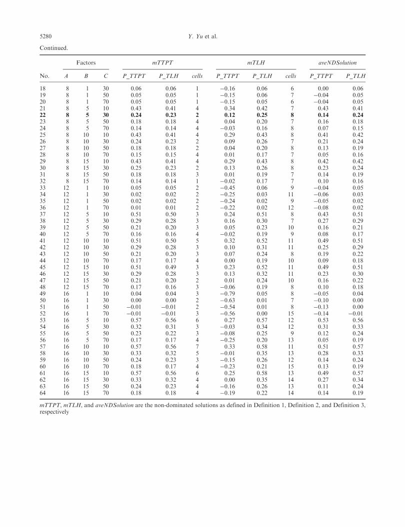
Continued.

Factors mTTPT mTLH aveNDSolution

No. A B C P_TTPT P_TLH cells P_TTPT P_TLH cells P_TTPT P_TLH

18 8 1 30 0.06 0.06 1 �0.16 0.06 6 0.00 0.0619 8 1 50 0.05 0.05 1 �0.15 0.06 7 �0.04 0.0520 8 1 70 0.05 0.05 1 �0.15 0.05 6 �0.04 0.0521 8 5 10 0.43 0.41 4 0.34 0.42 7 0.43 0.4122 8 5 30 0.24 0.23 2 0.12 0.25 8 0.14 0.2423 8 5 50 0.18 0.18 4 0.04 0.20 7 0.16 0.1824 8 5 70 0.14 0.14 4 �0.03 0.16 8 0.07 0.1525 8 10 10 0.43 0.41 4 0.29 0.43 8 0.41 0.4226 8 10 30 0.24 0.23 2 0.09 0.26 7 0.21 0.2427 8 10 50 0.18 0.18 2 0.04 0.20 8 0.13 0.1928 8 10 70 0.15 0.15 4 0.01 0.17 7 0.05 0.1629 8 15 10 0.43 0.41 4 0.29 0.43 8 0.42 0.4230 8 15 30 0.25 0.23 2 0.13 0.26 8 0.23 0.2431 8 15 50 0.18 0.18 3 0.01 0.19 7 0.14 0.1932 8 15 70 0.14 0.14 1 �0.02 0.17 7 0.10 0.1633 12 1 10 0.05 0.05 2 �0.45 0.06 9 �0.04 0.0534 12 1 30 0.02 0.02 2 �0.25 0.03 11 �0.06 0.0335 12 1 50 0.02 0.02 2 �0.24 0.02 9 �0.05 0.0236 12 1 70 0.01 0.01 2 �0.22 0.02 12 �0.08 0.0237 12 5 10 0.51 0.50 3 0.24 0.51 8 0.43 0.5138 12 5 30 0.29 0.28 3 0.16 0.30 7 0.27 0.2939 12 5 50 0.21 0.20 3 0.05 0.23 10 0.16 0.2140 12 5 70 0.16 0.16 4 �0.02 0.19 9 0.08 0.1741 12 10 10 0.51 0.50 5 0.32 0.52 11 0.49 0.5142 12 10 30 0.29 0.28 3 0.10 0.31 11 0.25 0.2943 12 10 50 0.21 0.20 3 0.07 0.24 8 0.19 0.2244 12 10 70 0.17 0.17 4 0.00 0.19 10 0.09 0.1845 12 15 10 0.51 0.49 3 0.23 0.52 11 0.49 0.5146 12 15 30 0.29 0.28 3 0.13 0.32 11 0.23 0.3047 12 15 50 0.21 0.20 2 0.01 0.24 10 0.16 0.2248 12 15 70 0.17 0.16 3 �0.06 0.19 8 0.10 0.1849 16 1 10 0.04 0.04 3 �0.79 0.05 8 �0.05 0.0450 16 1 30 0.00 0.00 2 �0.63 0.01 7 �0.10 0.0051 16 1 50 �0.01 �0.01 2 �0.54 0.01 8 �0.13 0.0052 16 1 70 �0.01 �0.01 3 �0.56 0.00 15 �0.14 �0.0153 16 5 10 0.57 0.56 6 0.27 0.57 12 0.53 0.5654 16 5 30 0.32 0.31 3 �0.03 0.34 12 0.31 0.3355 16 5 50 0.23 0.22 3 �0.08 0.25 9 0.12 0.2456 16 5 70 0.17 0.17 4 �0.25 0.20 13 0.05 0.1957 16 10 10 0.57 0.56 7 0.33 0.58 11 0.51 0.5758 16 10 30 0.33 0.32 5 �0.01 0.35 13 0.28 0.3359 16 10 50 0.24 0.23 3 �0.15 0.26 12 0.14 0.2460 16 10 70 0.18 0.17 4 �0.23 0.21 15 0.13 0.1961 16 15 10 0.57 0.56 6 0.25 0.58 13 0.49 0.5762 16 15 30 0.33 0.32 4 0.00 0.35 14 0.27 0.3463 16 15 50 0.24 0.23 4 �0.16 0.26 13 0.11 0.2464 16 15 70 0.18 0.18 4 �0.19 0.22 14 0.14 0.19

mTTPT, mTLH, and aveNDSolution are the non-dominated solutions as defined in Definition 1, Definition 2, and Definition 3,respectively

5280 Y. Yu et al.

Copyright of International Journal of Production Research is the property of Taylor & Francis Ltd and its

content may not be copied or emailed to multiple sites or posted to a listserv without the copyright holder's

express written permission. However, users may print, download, or email articles for individual use.

how to carry out assembly line–cell conversion? a

Documents