how sustainable are public debt levels in emerging europe?
TRANSCRIPT

48 FocuS on european economic integration Q4/12
How Sustainable are public Debt Levels in emerging europe?evidence for Selected ceSee countries from a Stochastic Debt Sustainability analysis
1 Motivation and BackgroundIn the face of the ongoing sovereign debt crisis in Europe, the sustainability of public finances has recently taken center stage in economics. The rapid buildup of government debt in an environment of financial instability and low growth has increased the need for a reliable and comprehensive assessment of government debt sustainability. This does not only hold for euro area countries, which are clearly the focus of today’s policy discussion, but also for countries in Central, Eastern and Southeastern Europe (CESEE). Empirical literature shows that sovereign debt levels tolerated by – in particular foreign – investors are lower for emerging countries than for advanced countries. According to the IMF (2003), public debt was below 60% of GDP in every second sovereign default case recorded in emerging market economies in the past.
Conceptually, debt sustainability is given as long as debt does not accumulate at a rate considerably exceeding the government’s capacity to service it (without
To assess to which extent public debt positions in four CESEE economies (the Czech Republic, Hungary, Poland and Slovakia) are sustainable in the medium term, we apply a stochastic debt sustainability analysis (SDSA), building on Celasun, Debrun and Ostry (2007). In contrast to conventional debt sustainability analyses, this approach explicitly accounts for the risks surrounding medium-term debt dynamics, e.g. risks stemming from the interaction of (endog-enously determined) fiscal and macroeconomic shocks. This is one of the first papers explicitly applying an SDSA to countries in emerging Europe. The baseline projections suggest that, on average, public debt would not get out of control in any of the four countries until 2016. How-ever, when we also account for the risks around the median projection, the primary balance is apparently not responsive enough (with regard to public debt) so that increasing debt paths cover a considerable share of the overall frequency distribution. The probability of reaching, in 2016, a higher debt-to-GDP ratio than in 2011 is largest in the Czech Republic and Slovakia and less pronounced in Hungary and Poland. When confronting the baseline projections with alternative policy scenarios, we can confirm the importance of a timely and continuous response to debt developments; otherwise public debt will quickly get out of control. Further-more, compliance with the defined Stability and Convergence Programme targets limits the overall risks to the debt outturns.
JEL classification: C54, E62, H63, H68, E62, P2Keywords: Public debt sustainability, fiscal reaction function, fan charts, stochastic simulations, public debt forecast, Central and Eastern Europe
Markus Eller, Jarmila Urvová1,2
1 Oesterreichische Nationalbank (OeNB), Foreign Research Division, [email protected] and [email protected] We are indebted to Marcos Rietti Souto, whose EViews program, which generates stochastic forecasts of the VAR
model, had been made available by the organizers of the Macro-Fiscal Modeling and Analysis course that took place at the Joint Vienna Institute in March 2012. For this paper, the program code was adjusted and developed further. We also thank two anonymous referees, Péter Benczúr (Magyar Nemzeti Bank), Jakob de Haan (De Nederlandsche Bank), Alex Mourmouras (IMF), Peter Backé, Martin Feldkircher, Pirmin Fessler, Doris Ritzberger-Grünwald, Tomáš Slacík (all OeNB), the participants of the conference “Fiscal Policy and Coordination in Europe” hosted by Národná banka Slovenska on September 13–14, 2012, and the participants of the 10th ESCB Emerging Markets Workshop hosted by the OeNB on October 4–5, 2012, for their valuable comments.

How Sustainable are public Debt Levels in emerging europe?
FocuS on european economic integration Q4/12 49
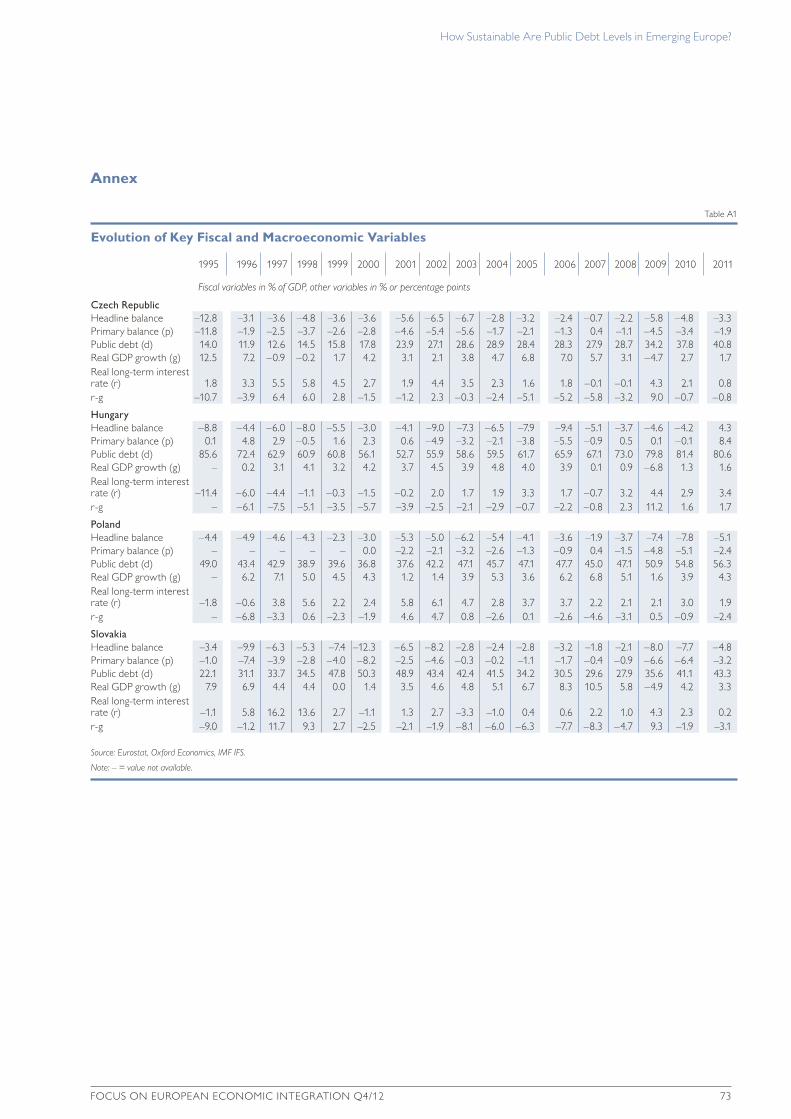
implausibly large policy adjustments, renegotiating or defaulting; see Ostry et al., 2010). Thus, the accumulated government debt has to be serviced at any point in time, which requires governments to be both solvent and liquid. A country faced with increasing difficulties in accessing financial markets in the short term could encounter debt sustainability problems over the medium term, as higher bond yields will gradually increase the cost of servicing debt. Before the outbreak of the global financial crisis, debt levels of CESEE countries were indeed comparatively low and thus seemed manageable. Then, debt, however, quickly rose to unexpect-edly high levels (see table A1 in the annex). As foreign investors changed their risk assessment in the wake of the collapse of Lehman Brothers, some CESEE coun-tries, such as Hungary, Latvia or Romania, even lost market access and had to resort to the IMF and the EU for multilateral assistance (see Eller, Mooslechner and Ritzberger-Grünwald, 2012).
Depending on the chosen time horizon, the literature distinguishes between three different forward-looking approaches to measuring debt sustainability: (1) short-term approaches, where refinancing profiles are examined to assess liquidity and roll-over risks; (2) medium-term approaches, where both debt trajectories and changes in these trajectories under different scenarios are projected for about 5 to 15 years ahead; and (3) long-term approaches, where sustainability gaps are calculated for several decades ahead and the budgetary impact of demographic changes, such as aging societies (e.g. Balassone et al., 2011) is examined. For our analysis, we chose to implement a medium-term methodology.
Among the class of medium-term approaches, “conventional” (deterministic) debt sustainability analysis (DSA) has become a core element of enhanced country surveillance (contained in the IMF’s Article IV staff reports). This type of analysis is, however, mainly an accounting exercise based on the standard debt accumula-tion equation. As such it is subject to several limitations. For instance, the standard debt accumulation equation abstracts from interdependencies between its key determinants: GDP growth, interest rates and primary balances. This can lead to an underestimation of the risks to the projected debt path, as was also pointed out by the IMF (2008) itself.3 Moreover, medium-term debt trajectories are surrounded by a high degree of uncertainty, which in the conventional DSA is usually not taken into account. Stochastic approaches, as developed by Celasun, Debrun and Ostry (2007), capture the interaction among the determinants of public debt dynamics and are meant to enhance the understanding of the risks and their magnitude surrounding medium-term debt projections. This way, the proba-bilistic nature of debt sustainability analysis exercises is explicitly acknowledged. Within a stochastic approach, the reference (baseline) scenario is illustrated in fan charts, which depict confidence bands for varying degrees of uncertainty around the median projection. The confidence bands are wider for countries for which uncertainty about medium-term debt developments is higher than for countries with a more muted risk of debt sustainability. In the same vein, fan charts make it possible to quantify the probability that the debt ratio will turn out higher or lower than a certain value.
3 “It is important to emphasize that the results are not full-fledged scenarios, as there is no interaction among variables. [… ] This implies the need to interpret the stress tests with a grain of salt.” (IMF, 2008, p. 6).

How Sustainable are public Debt Levels in emerging europe?
50 FocuS on european economic integration Q4/12
We believe that the stochastic debt sustainability analysis (SDSA) approach is especially suitable for the CESEE countries. Like other emerging market econo-mies (see Alvarado, Izquierdo and Panizza, 2004), they are subject to a consider-ably volatile economic environment (e.g. due to sudden stops and goes of external financing). Such an environment has immediate consequences for the government budget (e.g. revenue windfalls during boom years) and translates into a higher degree of uncertainty of the public debt sustainability assessment. We thus build on the work by Celasun, Debrun and Ostry (2007) and produce an SDSA for four CESEE economies: the Czech Republic, Hungary, Poland and Slovakia. Except for Medeiros (2012), who provided some evidence for Poland, Slovakia and Slovenia, we have not yet found a paper with an application of the SDSA framework to CESEE economies.
In line with Celasun, Debrun and Ostry (2007), we combine the estimation of a fiscal reaction function (primary balance as a function of debt and output gap) with the estimation of an unrestricted VAR model for nonfiscal macroeconomic variables to come up with debt path projections. The baseline projection of the debt-to-GDP ratio is subject to both random fiscal and macro shocks. Thus, fiscal policymakers can react to macro shocks endogenously. Frequency distributions of the debt ratio can then be obtained for each year of projection and used to draw fan charts. Besides applying this framework to CESEE countries, we try to add to the existing literature by (1) confronting the baseline projections with various alternative policy scenarios (essentially different types of fiscal policy response), (2) experimenting with additional determinants in the fiscal reaction function and (3) carefully addressing, in the VAR model, the properties of the underlying time series, in particular their nonstationarity.
The remainder of this paper is structured as follows: Section 2 defines debt sustainability and delineates the building blocks of the chosen SDSA framework. Section 3 shows the empirical specification and the results for the estimation of the fiscal reaction function. Section 4 discusses the structure and the selection of the VAR model for the nonfiscal macroeconomic determinants of public debt dynamics. By means of fan charts, section 5 illustrates the core results of our paper: the projected public debt paths for the four CESEE economies until 2016 under different scenarios. Section 6 stresses some caveats related to the SDSA approach and points to the need for further research in the field. Finally, the basic findings and their implications for policymaking are summarized in section 7. Definitions and sources of the data used in sections 3 and 4 are shown in the annex (tables A2.1 and A2.2).
2 Definition of Debt Sustainability and Description of the Chosen Methodological Framework
First of all, we need a definition of debt sustainability in our setting and a description of the building blocks of the applied SDSA framework to provide a methodological anchor for the results presented in the subsequent sections.

How Sustainable are public Debt Levels in emerging europe?
FocuS on european economic integration Q4/12 51
2.1 Definition of Debt Sustainability Consider the following law of motion for the evolution of public debt over time:
Dt = 1+ it( )Dt−1−PBt + St (1)
where Dt is the stock of public debt maturing at the end of period t, it denotes the one-period nominal interest rate, PBt = Rt – Gt is the primary balance (the difference between total government revenues and noninterest government spending), and St represents stock-flow adjustments (e.g. contingent liabilities or extra revenue stemming from privatizations).
Assuming that St = 04 and dividing equation (1) by nominal GDP (price level times real GDP) yields:
DtPtYt=
(1+ it )(1+πt )(1+ gt )
Dt−1Pt−1Yt−1
−PBtPtYt= dt =
1+ rt( )1+ gt( )
dt−1− pt
(2)
where dt is the debt-to-GDP ratio, pt is the primary balance-to-GDP ratio, rt is the real interest rate, πt is the inflation rate and gt is the real GDP growth rate. Under the assumption that rt , gt and pt remain constant over time, it is evident from equation (2) that the debt-to-GDP ratio remains stable as long as
θ=1+ r( )1+ g( )
≤1 .
If θ>1 , i.e. r> g (the often-quoted positive interest-growth differential), a suffi-ciently positive primary balance-to-GDP ratio is needed to keep the debt ratio stable.5 Because the assumption of constant variables over time is not very realistic, our approach allows for stochastic changes in these variables during the forecasting horizon.
Strict debt sustainability would require, first, that debt is repaid in the very end, i.e.
limt→∞E dt( )= 0
(no-Ponzi-game condition) and, second, that in a stochastic world the distribution of all possible realizations of dt does not exceed any finite limit, i.e. the expected variance of dt is asymptotically finitelimt→∞E σdt
2( )<∞ .
4 Table A3 shows that stock-flow adjustments in the four CESEE countries under investigation are on average comparatively small. However, they are also rather erratic over time. It would thus be important to capture that in the debt projections as well (if respective data were available). In section 6, in an alternative policy scenario (Structural and Convergence Programme targets), we account for planned stock-flow adjustments in those countries for which we have the respective information.
5 Interestingly, as can be seen from table A1, of the four countries under review, only Hungary managed to produce primary surpluses in years with a positive interest-growth differential. Despite the sizeable positive interest-growth differential, there was still a considerable primary balance deficit in the Czech Republic in the years 1997–99, 2002 and 2009, in Poland from 2001 until 2003 and in Slovakia in the years 1997–99 and 2009. It is also evident from table A1 that the debt-to-GDP ratio increased quite strongly during these years of a mismatch between pt and rt – gt.

How Sustainable are public Debt Levels in emerging europe?
52 FocuS on european economic integration Q4/12
Unfortunately, these definitions are not very useful in empirical applications, as it is not possible to make forecasts over an infinite horizon. Ferrucci and Penalver (2003) thus proposed a weaker definition: Debt is sustainable as long as there is a reasonably high probability that dt is not higher at the end of the forecast horizon than at the beginning. When interpreting our results in section 5, we follow this reasoning and show the probabilities of exceeding a given debt value by 2016.
2.2 Building Blocks of the SDSA Framework
The SDSA framework consists of three building blocks: a fiscal reaction function, a VAR model and the traditional debt accounting identity. The first and the last block use annual data, as reliable fiscal accrual variables and control variables in the fiscal reaction function (e.g. institutional variables) are more readily available on an annual basis. The VAR model, on the other hand, works with quarterly macroeconomic data, which are annualized before entering the debt identity. This feature makes the framework suitable for emerging market economies, as for these countries the available economic time series are often short. Utilizing higher- frequency data thus helps overcome this problem to a certain extent. In this section, we briefly discuss each of the three building blocks and follow the nota-tion of Celasun, Debrun and Ostry (2007).
2.2.1 Debt-Deficit Stock-Flow Identity
To account for the considerable share of public debt denominated in foreign currency in the countries under investigation, we rewrite equation (2) for a sover-eign issuing bonds in foreign currency:
dt ≡ 1+ gt( )−1 1+ rt f( ) 1+∆ zt( )dt−1f + 1+ rt( )dt−1d⎡⎣⎢
⎤⎦⎥− pt
(3)
where, besides the notation already explained for equation (2), rtf denotes the real
foreign interest rate, rt the real domestic interest rate, ∆zt is the rate of depreciation of the (log of the) real effective exchange rate, d f
t–1 is the foreign currency-denom-inated debt-to-GDP ratio6 and dd
t–1 captures debt denominated in domestic cur-rency.
To come up with a projection of dt for future periods (our forecasts run from 2012 to 2016), we first need to obtain projections of the underlying debt identity variables in equation (3). In the SDSA framework, forecasts of the primary balance are obtained through a fiscal reaction function and forecasts of the macro-economic variables rt
f, rt ,gt ,∆ zt are obtained through a VAR model.
2.2.2 Fiscal Reaction Function (FRF)
The fiscal reaction function endogenizes fiscal policy so that the policymaker reacts to the business cycle, past level of debt and a set of controls (e.g. inflation or the election cycle). Policy persistence is captured by the lagged primary balance term on the right-hand side. Fiscal policy thus becomes a source of uncertainty
6 When generating the debt simulations, we take for each year in the forecasting period the average share of foreign currency-denominated public debt in total public debt in the years 2010 and 2011.

How Sustainable are public Debt Levels in emerging europe?
FocuS on european economic integration Q4/12 53
about the debt level, in as much as it deviates from the behavior predicted by the FRF. We estimate the reaction function as follows:
pi,t =α0+δ pi, t−1+ρdi, t−1+k=0
1
∑γkogi,t−k + Xi, tβ+ηi+εi, t
(4)
t = 1,…,T, i = 1,…,N
where pi,t is the ratio of the primary balance to GDP in country i and year t, di,t–1 is the public debt-to-GDP ratio observed at the end of the previous year, ogi,t is the output gap, ηi is an unobserved country fixed effect, Xi,t is a vector of control variables and εi,t ~ iid(0,σ2
ε ).
2.2.3 Simulated Forecasts of the Primary Balance
The estimated FRF is used to generate forecasts of the primary balance for the period 2012 to 2016, which are obtained as follows:
pi,t+τ =Λi, t+τ + δ pi, t+τ−1+ ρdi, t+τ−1+
k=0
1
∑γkogi,t+τ−k +ϕi, t+τ
(4.1)
τ = 1,…,5
Λi, t+τ = pi,t− δ pi, t−1− ρdi, t−1−k=0
1
∑γkogi,t−k = α0+ Xi, tβ+ ηi (4.1.1)
ϕi, t+τ = σ ηi+εi , t( )2 υt+τ (4.1.2)
υt+τ ~ N 0, 1( ) and ϕi, t+τ ~ N 0, σ
ηi+εi , t( )2( ) (4.1.3)
Λi,t+τ captures the impact of all determinants of the primary surplus other than the lagged primary balance, lagged debt and the output gap and represents a country-specific constant component of the primary balance.
φi,t+τ is a random draw from a set of 1,000 shocks with a mean-zero normal distribution and a variance equal to the country-specific variance of the FRF residuals (ηi + εi,t ).7 A set of 1,000 forecasts of the primary balance, in line with these stochastic shocks, is generated from equation (4.1).
Note that the primary balance forecasts also depend on future realizations of the output gap, which, in turn, are affected by the macroeconomic shocks obtained with the VAR model. This implies that the fiscal policymaker responds to macro shocks during the forecasting horizon; in contrast to the deterministic DSA, we therefore allow for an endogenous fiscal policy.
7 If stock-flow adjustments materialized in the past, they are captured as part of εi,t and thus affect the variability of the fiscal shocks. This implies that past stock-flow adjustments still translate to a certain extent into projected primary balances and thus projected debt levels.

How Sustainable are public Debt Levels in emerging europe?
54 FocuS on european economic integration Q4/12
2.2.4 Unrestricted VAR Model for Nonfiscal Determinants of Public Debt DynamicsFor each country, a VAR model with the macroeconomic determinants of the debt dynamics is estimated based on quarterly data:
Yt = γ0+k=1
p
∑γkYt−k +ξt
(5)
where Yt = (rtf, rt , gt , ∆zt ), γk is a vector of coefficients and ξt ~ N(0, Ω) is a vector of
well-behaved error terms with a variance-covariance matrix Ω.
2.2.5 Simulated Forecasts of the Macroeconomic Variables from the VAR Model
Based on the variance-covariance matrix Ω of the VAR model, a sequence of 1,000 random vectors ξτ is generated in a similar vein as in the FRF simulations. Thus, the sequence of random vectors corresponds to ξt+τ = Wυt+τ , ∀τ∈[t + 1, T], where υt+τ ~ N(0,1) and Ω = W'W (υt+τ is a random draw from a standard normal distribution and W is the Choleski factorization of Ω). Consequently, a set of 1,000 forecasts of the macroeconomic variables is generated by the VAR model such that a joint dynamic response of the variables is warranted.
Yt+τ = γ0+γ1Yt+τ−1+ξt+τ
(5.1) τ=1,…,5
The projections of the macroeconomic variables that contain the stochastic shocks are then annualized and – together with the primary balance forecasts containing fiscal stochastic shocks – enter the debt-deficit stock-flow identity to generate the debt projections.
3 Average Fiscal Policy Patterns: Fiscal Reaction Function
The main goal of estimating the fiscal reaction function (equation (4)) lies in obtaining a prediction of the primary budget balance-to-GDP ratio. We estimate the FRF for a panel of eight CESEE countries (CESEE-8: Bulgaria, Croatia, the Czech Republic, Hungary, Poland, Romania, Slovakia, Slovenia) and a maximum of 17 years (1995–2011).8 For the FRF estimation, we use a – compared with the whole SDSA exercise – broader sample of rather homogeneous countries (in line with Staehr, 2008; Abiad and Ostry, 2005; or Ostry et al., 2010) to address the lack of sufficiently long fiscal time series in the countries under consideration.
3.1 Empirical Specification of the Fiscal Reaction Function
The fiscal reaction function shows the response of the primary budget balance-to-GDP ratio9 to a set of macroeconomic and institutional variables, of which the
8 To account for the problem of data outliers, we corrected the 2011 primary balance of Hungary for one-off measures, which – according to the Convergence Programme submitted to the European Commission – amounted to 9.4% of GDP.
9 In line with the existing literature (e.g. Bohn, 1998, or Ostry et al., 2010), we use the overall primary balance, and not the cyclically adjusted one, as dependent variable given that the unadjusted primary balance is relevant for calculating the debt evolution. This has, of course, the drawback that we cannot disentangle the policymaker’s direct reaction – i.e. discretionary part – from budgetary items changing automatically due to business cycle fluctuations (automatic stabilizers).

How Sustainable are public Debt Levels in emerging europe?
FocuS on european economic integration Q4/12 55
debt-to-GDP ratio and the output gap are the most important ones. A positive response of the primary balance to lagged debt can be expected if buoyant debt dynamics are corrected. If the primary balance were related positively to the out-put gap, favorable economic developments would improve the budgetary position of a country (e.g. via boom-induced revenue windfalls) – indicating a countercyclical fiscal response. By contrast, a negative coefficient would indicate a procyclical, and an insignificant coefficient an acyclical fiscal response. We included lagged output gaps to account for any persistent impact of recessions and booms.
To better explain the evolution of – and thus to improve – the fit of the primary balance ratio, we experimented with the inclusion of various additional explanatory variables, which might induce a reaction by the fiscal policymaker or determine the surplus-generating capacities of a country. Obvious candidates are: (1) the lagged primary balance to account for policy persistence; (2) the inflation rate; (3) the quality of fiscal institutions, existing fiscal rules; (4) political events like elections: different types of election dummies10; (5) foreign business cycle shocks (either via trade openness or via the growth differential vis-à-vis the main trading partners); or (6) other factors such as revenue windfalls, natural disasters, large-scale infrastructure investments, social security reforms. We included a variety of these control variables in several robustness checks. (1) and (2) remained robust across various specifications. For (3) to (5) we included several indicators, which, as they did not turn out to be significant, are not included in the final estimations (e.g., elections showed the expected negative sign but were only signi-ficant at the 80% level). Ideally, one would also include data or proxies for (6), but due to data constraints, we had to abstain so far from doing so.
We depart from Celasun, Debrun and Ostry (2007) by including the lagged primary balance, lagged output gaps or the inflation rate. On the other hand, several additional explanatory variables, which they had found significant for a broad set of emerging economies, including the Latin American countries, turned out to be insignificant for our set of CESEE countries (e.g. institutional variables). This suggests that fiscal policy in the CESEE countries is, to a certain extent, determined by factors that differ from those of their emerging peers. Moreover, we experimented with different output gap definitions: based on trend GDP and on potential GDP (both from the European Commission) and based on a Hodrick-Prescott-filtered GDP series (with a smoothing parameter of 6.25 as recom-mended by Ravn and Uhlig (2002) for annual figures). The latter definition was favored in our benchmark regression.
The lagged primary balance was included to appropriately account for the autocorrelation of the residuals, i.e. to get a dynamic version of the panel. As it is well established in the literature (e.g. Nickell, 1981), estimates of the lagged dependent variable are likely to be biased in short-T samples. Moreover, there are also reasonable arguments that the output gap and the lagged debt ratio are endogenous regressors (e.g. IMF, 2003). Therefore, we work – besides the fixed effects panel specification (FE) – also with GMM techniques designed for dynamic panels (system GMM estimator of Blundell and Bond, 1998). Despite the theo-
10 To address the potential endogeneity bias from reverse causation or from shocks affecting both the election date and the fiscal balance, we separate out those elections whose timing is predetermined (in line with Shi and Svensson, 2006) and distinguish between pre- or early election years and full-blown election years (see table A2.1).

How Sustainable are public Debt Levels in emerging europe?
56 FocuS on european economic integration Q4/12
retical advantages of the system GMM estimator, we eventually opted for the panel fixed effects estimator (column (2) in table 1) as our baseline for the subsequent calibrations.
The following considerations guided our choice: First, in the GMM setting, the minimal number of required instruments turns out to be large relative to the number of observations (although we collapsed instruments and used only a limited number of lags of the endogenous variables as instruments). Roodman (2009) stressed that instrument proliferation can overfit endogenous variables, fail to expunge their endogenous components and weaken the power of the Hansen instrument validity test (a telltale sign is the perfect Hansen p-value of 1.0). Second, as also elaborated in Roodman (2009), reliable estimates of the true parameter (of the lagged dependent variable) should lie in or near the “credible” range between pooled OLS and the panel fixed effects estimator. As can be seen in table 1, the system GMM estimator for δ still comprises, in its 95% confidence interval, the pooled OLS estimator and thus is not too far away from the credible range. More-over, considering again a 95% confidence interval around the estimates, the pooled OLS and the fixed effects estimator cannot really be distinguished from each other. Therefore, at least in statistical terms, we cannot argue that the coefficients estimated with the three different methodologies are really different from each other; the bias due to endogeneity in the favored FE specification should thus be limited.
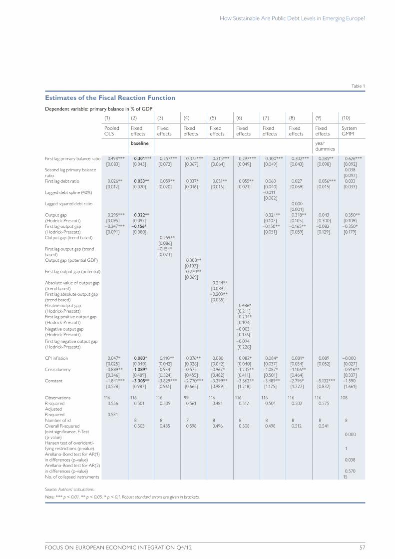
3.2 Estimation Results
The results of the baseline specification are shown in table 1. The primary balance shows a great deal of persistence. If the primary balance-to-GDP ratio improves by 1% of GDP in year t, it improves by a further 0.3% of GDP in year t+1.
The positive coefficient for the debt-to-GDP ratio implies that the primary balance improves when last year’s debt ratio increased. If debt increases by, say, 10 percentage points of GDP, one year later the primary balance strengthens by about 0.5% of GDP (if the debt ratio increases from, for instance, 60% to 70% in year t, the primary deficit ratio will shrink from, for instance, –3.0% to –2.5% in year t+1). Later we also experiment with a stronger response and examine its impact on the evolution of future debt paths.
Several scholars have investigated potential nonlinearities between the primary balance and the debt ratio. An obvious prior would be that the responsiveness of the primary balance is stronger at high than at low debt ratios. Apparently, this hypothesis can only be verified for advanced economies (where the responsiveness is stronger once debt surpassed 80% of GDP, see IMF, 2003), while in emerging markets the marginal responsiveness of the primary balance to high debt levels decreases (see Abiad and Ostry, 2005, or IMF, 2003). Possible reasons are limited fiscal consolidation capacities in emerging economies at high debt levels, weak revenue bases (lower yields, higher volatility) due to tax evasion as well as less effectiveness at controlling government spending during boom times (limited fiscal space). We experimented with a threshold of 40% in column (7) and with a squared debt ratio in column (8) of table 1. Based on these results, we cannot verify that nonlinearities are present in our sample. At least the negative sign for the 40% debt threshold is in line with the evidence mentioned for emerging economies.
How Sustainable are public Debt Levels in emerging europe?
FocuS on european economic integration Q4/12 57
table 1
Estimates of the Fiscal Reaction Function
Dependent variable: primary balance in % of GDP
(1) (2) (3) (4) (5) (6) (7) (8) (9) (10)
pooled oLS
Fixed effects
Fixed effects
Fixed effects
Fixed effects
Fixed effects
Fixed effects
Fixed effects
Fixed effects
System gmm
baseline year dummies
First lag primary balance ratio 0.498*** 0.301*** 0.257*** 0.375*** 0.315*** 0.297*** 0.300*** 0.302*** 0.285** 0.626***[0.083] [0.045] [0.072] [0.067] [0.064] [0.049] [0.049] [0.043] [0.098] [0.092]
Second lag primary balance ratio
0.038[0.097]
First lag debt ratio 0.026** 0.053** 0.059** 0.037* 0.051** 0.055** 0.060 0.027 0.056*** 0.033[0.012] [0.020] [0.020] [0.016] [0.016] [0.021] [0.040] [0.069] [0.015] [0.033]
Lagged debt spline (40%) –0.011[0.082]
Lagged squared debt ratio 0.000[0.001]
output gap (Hodrick- prescott)
0.295***[0.095]
0.322**[0.097]
0.324**[0.107]
0.318**[0.105]
0.043[0.300]
0.350**[0.109]
First lag output gap (Hodrick-prescott)
–0.247***[0.091]
–0.156*[0.080]
–0.150**[0.051]
–0.165**[0.059]
–0.082[0.129]
–0.350*[0.179]
output gap (trend based) 0.259**[0.086]
First lag output gap (trend based)
–0.154*[0.073]
output gap (potential gDp) 0.308**[0.107]
First lag output gap (potential) –0.220**[0.069]
absolute value of output gap (trend based)
0.244**[0.089]
First lag absolute output gap (trend based)
–0.209**[0.065]
positive output gap (Hodrick-prescott)
0.486*[0.211]
First lag positive output gap (Hodrick-prescott)
–0.234*[0.103]
negative output gap (Hodrick-prescott)
–0.003[0.176]
First lag negative output gap (Hodrick-prescott)
–0.094[0.226]
cpi inflation 0.047* 0.083* 0.110** 0.076** 0.080 0.082* 0.084* 0.081* 0.089 –0.000[0.025] [0.040] [0.042] [0.026] [0.042] [0.040] [0.037] [0.034] [0.052] [0.027]
crisis dummy –0.889** –1.089* –0.934 –0.575 –0.967* –1.235** –1.087* –1.106** –0.916**[0.346] [0.489] [0.524] [0.455] [0.482] [0.411] [0.501] [0.464] [0.337]
constant –1.841*** –3.305** –3.829*** –2.770*** –3.299** –3.562** –3.489** –2.796* –5.132*** –1.590[0.578] [0.987] [0.961] [0.665] [0.989] [1.218] [1.175] [1.222] [0.832] [1.661]
observations 116 116 116 99 116 116 116 116 116 108r-squared 0.556 0.501 0.509 0.561 0.481 0.512 0.501 0.502 0.575adjusted r-squared 0.531number of id 8 8 7 8 8 8 8 8 8overall r-squared 0.503 0.485 0.598 0.496 0.508 0.498 0.512 0.541Joint significance, F-test (p-value)
0.000
Hansen test of overidenti- fying restrictions (p-value) 1arellano-Bond test for ar(1) in differences (p-value) 0.038arellano-Bond test for ar(2) in differences (p-value) 0.570no. of collapsed instruments 15
Source: Authors’ calculations.
Note: *** p < 0.01, ** p < 0.05, * p < 0.1. Robust standard errors are given in brackets.

How Sustainable are public Debt Levels in emerging europe?
58 FocuS on european economic integration Q4/12
While the contemporaneous output gap shows a positive sign (irrespective of the method used for calculating the output gap), the first lag shows a negative sign. This indicates that the primary budget has a countercyclical effect in the year the business cycle position changes (probably due to a predominant impact of built-in automatic stabilizers), while in the following year we can observe a procyclical response (probably due to delayed discretionary fiscal policy responses). These results do not change when different output gap definitions are used (see columns (3) to (5)). Interestingly, the results are particularly pronounced for boom periods, while during economic downturns there seems to be no impact (see column (6), where we distinguished between periods with positive and negative output gaps).
One might take the view that the set of countries contained in this panel esti-mation is already too heterogeneous in terms of fiscal policymaking, given that two of them (Slovakia and Slovenia) already joined the euro area or that debt-to-GDP ratios are fairly different across countries. To address the issue of panel heterogeneity, we reran the FRF by excluding each country one by one.11 The resulting coefficients still lied within a 95% confidence interval around the CESEE-8 baseline estimates. Bulgaria and Hungary are outliers in the sense that the coefficients without Bulgaria are in most cases systematically larger and with-out Hungary systematically smaller than in the baseline (reflecting the fact that the debt ratio in both countries differs substantially from the average debt ratio in the CESEE-8). Nonetheless, when we excluded both Hungary and Bulgaria at the same time, the resulting coefficients still lied within the 95% confidence interval around the CESEE-8 estimates. For this reason, we believe that the subsequent calibration of the primary balance projections for the Czech Republic, Hungary, Poland and Slovakia is appropriate.12
4 Nonfiscal Determinants of Public Debt Dynamics: VAR Model
The aim of the VAR model in the SDSA framework (equation (5)) is to provide a forecast of the macroeconomic determinants of public debt, so that they are contemporaneously correlated and persistent. The SDSA also captures the uncer-tainty related to this forecast and the resulting debt path. This is achieved by gen-erating not one, but many (in our case 1,000) possible sets of projections of growth, the exchange rate and the domestic and foreign interest rates. These projections incorporate shocks drawn from the joint distribution of the variables, whose mean and variance-covariance matrix were estimated from the historical data with the VAR model.
For each country, we estimate a VAR model with quarterly macroeconomic data (1995Q1–2011Q4 for Slovakia and the Czech Republic, and 1996Q1–2011Q4 for Poland and Hungary13). The length of the available time series imposes a limit on the number of lags in the VAR model we can realistically use; therefore we restrict our analysis to models with one lag only, similarly to Celasun, Debrun and Ostry (2007). Moreover, it has been argued (e.g. Hafer and Sheehan, 1989) that short-lagged VAR models tend to be more accurate, on average, when used for
11 Results are available from the authors upon request.12 For Hungary, one could opt for somewhat larger parameter values than the CESEE-8 baseline results would
suggest. Nevertheless, there is no straightforward approach to determining such a markup.13 The different sample lengths are due to data availability.

How Sustainable are public Debt Levels in emerging europe?
FocuS on european economic integration Q4/12 59
forecasting, than longer-lagged models. However, adding one or two lags in a robustness check exercise did not substantially change the results, except in the case of Hungary, where one additional lag brought the baseline median debt projection down by 4 percentage points.
Output, interest rates and exchange rates are often found to be nonstationary. We therefore test each time series used in the model for the presence of a unit root with an Augmented Dickey-Fuller test, supplemented by the Phillips-Perron test.14 We cannot reject the null hypothesis of nonstationarity of the foreign real interest rate and of the Hungarian domestic real interest rate. These results hold for various sample periods, e.g. when the observations at the beginning or at the end of the sample are cut off based on the consideration that the transformation period still under way at the end of the 1990s or the current crisis may distort the results. Differenced series exhibit no unit root, therefore we conclude that they are integrated of order one (I(1)). After similar considerations (i.e. accounting for the effects of the crisis and/or transformation period), we decided to treat the Slovak, Polish and Czech domestic interest rates as stationary, as we did not find strong enough evidence of the presence of a unit root at the 99% confidence level. The GDP and real effective exchange rate variables enter the models as differences and these differences are found to be stationary, in line with our expectations.
In a next step, we test each of the models (in levels) for cointegration, using the Johansen procedure. We do not find evidence for the presence of one or more cointegrating relationships both according to the maximum eigenvalue and the trace test statistics. Therefore, we proceed by estimating an unrestricted VAR(1) model for each country, whereby the variables, which were found to be integrated of order one, are differenced. Even though a regression of an interest rate in differ-ences on an interest rate in levels is not derived from economic theory, it is crucial to address the nonstationarity of the data, which is done by differencing. However, differencing also means losing part of the information contained in the data, and to avoid “overdifferencing,” we only differenced those variables which were found to be I(1).
As a kind of a robustness check, we also estimate the VAR models for shorter time-series samples (e.g. starting in 1998, due to the above-mentioned trans-formation period and possible structural break considerations). Their results have to be treated with caution, though, as by doing so, we also lose a considerable number of degrees of freedom. We find that the median projection and the range of the projections remain broadly unchanged for all the countries, except for the Czech Republic, where a shorter sample raises the median projection by about 5 percentage points. This is possibly due to the sensitivity of the Czech model to the pronounced crisis period at the end of the sample.
The detailed estimation output for the chosen VAR models is shown in the annex (tables A4.1 to A4.4). While the explanatory power of the regressors for GDP growth and the domestic interest rate is in most of the cases very satisfac-tory, it is rather limited for the foreign interest rate and partly also for the real effective exchange rate. This is, however, not very surprising given that these variables depend more on economic developments abroad and our small VAR
14 Available from the authors upon request.

How Sustainable Are Public Debt Levels in Emerging Europe?
60 FocuS on EuroPEAn Economic intEgrAtion Q4/12
model is not able to account for that. Keeping the VAR model small is necessary owing to the limited number of observations. At the same time, as can be seen from table A5, it produces simulations which show a reasonable size and variation (given historical values and comparable data from the IMF’s Article IV staff reports) and this is the most important issue for the subsequent debt projections.
5 Projected Public Debt Paths and Risks to Debt Sustainability
In this section, we put all the ingredients from section 3 (endogenous fiscal policy) and section 4 (description of the nonfiscal macroeconomic environment) together to generate, by means of stochastic simulations, a large sample of debt paths for a five-year-ahead forecasting horizon for the Czech Republic, Hungary, Poland and Slovakia. Different debt paths are generated by two types of shocks: macro shocks (drawn from a joint distribution) stem from the VAR model and fiscal shocks from the estimated fiscal reaction function.
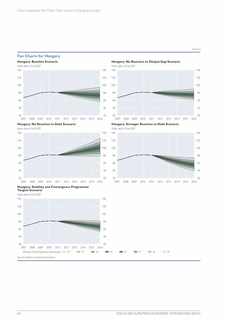
The fan charts shown in this section (charts 2 to 6) summarize the frequency distribution of the projected debt paths and serve to illustrate the overall range of risks to the debt dynamics in our sample. The median projection (black line in the center of the fan) connects the median values of the frequency distributions for each year in the forecasting period (i.e. in a given year, 50% of the debt projec-tions lie below and 50% above this reference value). Stepwise shaded areas capture different deciles of the frequency distribution. For instance, the darkest shaded area reflects debt paths located in the 5th and 6th deciles of the distribution, thus representing a 20% confidence interval around the median projection. The overall colored cone, in turn, reflects the 2nd to 9th deciles of the distribution and depicts a confidence interval of 80% around the median projection.
For each country we experiment with five different policy scenarios, which basically correspond to different calibrations of the estimated fiscal reaction function. In charts 2 to 5, from the upper left-hand corner to the lower right-hand one, we start with the baseline scenario, where the primary balance is calibrated in line with the favored FRF estimates (column (2) in table 1). In the second scenario, we only set the output gap coefficients γk in equation (4.1) to zero, i.e. we examine a situation where the primary balance does not react to business cycle fluctuations (acyclical behavior). In a similar vein, in the third scenario, we only set the coefficient for lagged debt ρ to zero. An increase in the primary balance is thus no longer the case when debt increases, i.e. we examine a situation where the government does not react timely and continuously to rising debt levels. In contrast, in the fourth scenario, we assume a coefficient for lagged debt which is twice as high as in the baseline (ρ =0.1). Finally, in the fifth scenario, we replace in equation (4.1) the fit for the primary balance with the governments’ yearly primary balance targets for 2012 to 2015 (for 2016 we assume the same value as in 2015), still allowing for unexpected, stochastic shocks originating from the fiscal reaction function15, i.e.
15 We still allow the residuals of the FRF to enter the debt-deficit stock-flow identity, i.e. the debt evolution is subject to stochastic fiscal shocks, which cannot be traced back to the variables that were included as regressors in equation (4). An example would be erratic policy actions or one-off events, such as natural disasters, that trigger an unexpected change in the primary balance.

How Sustainable are public Debt Levels in emerging europe?
FocuS on european economic integration Q4/12 61
pb i,t+τ = SCP targeti,t+τ +ϕi, t+τ . (6)
Whenever available, also the planned stock-flow adjustments are included (based on the Stability and Convergence Programmes (SCPs) submitted to the European Commission in April 2012; for more details, see table 2). Uncertainty around the median debt projection is triggered in this scenario mainly by the macro shocks and not by systematic fiscal policy deviations. This scenario gives information about how effectively the defined targets contribute to the stabilization of debt levels until 2016.
First of all, let us focus on the preferred baseline scenario. When we draw our attention to the median projections, we can observe an increasing median debt path in the Czech Republic and Slovakia, whereas that in Hungary and Poland shows a downward sloping trend. Altogether, these median projections do not indicate that public debt gets out of control until the end of the forecasting horizon and can thus be qualified to be sustainable over the period from 2012 to 2016. However, when we also take the risks around the median projection into account, we get a more differentiated picture. The fiscal reaction function is apparently not responsive enough (with regard to public debt) to prevent increasing debt paths from covering a considerable share of the overall frequency distribution. Chart 1 illustrates (analogously to Medeiros, 2012) for each country the empirical proba-bilities of exceeding a given debt value by 2016. The probability of having in 2016 a higher debt ratio than in 2011 is largest in the Czech Republic (76%) and in
table 2
Target Primary Balances of Individual Countries (2012–2015) Used in the Stability and Convergence Programmes
2012 2013 2014 2015 average
% of GDP
Czech Republictarget primary balance –1.5 –1.3 –0.1 0.8 –0.5planned stock-flow adjustment (SFa)1 0.7 –0.7 –0.5 –0.5 –0.3primary balance adjusted for the SFa –2.2 –0.6 0.4 1.3 –0.3
Hungarytarget primary balance 1.6 2.0 2.2 2.2 2.0planned stock-flow adjustment (SFa)1 – – – – –primary balance adjusted for the SFa 1.6 2.0 2.2 2.2 2.0
Polandtarget primary balance –0.2 0.5 1.0 1.6 0.7planned stock-flow adjustment (SFa)1 – – – – –primary balance adjusted for the SFa –0.2 0.5 1.0 1.6 0.7
Slovakiatarget primary balance –2.9 –2.5 –2.1 –1.5 –2.3planned stock-flow adjustment (SFa)1 3.6 1.3 1.6 0.6 1.8primary balance adjusted for the SFa –6.5 –3.8 –3.7 –2.1 –4.0
Source: Stability and Convergence Programmes 2012, Commission Staff Working Documents – Assessments of the 2012 National Reform Rrogrammes and Stability Programmes 2012.
1 Does not include revaluation effects due to exchange rate movements, as the exchange rate revaluation effects are factored into the debt simulations. For Hungary and Poland, no detailed information about what fraction of the SFA is due to exchange rate movements was available in the Stability and Convergence Programmes, which is why we did not include the SFA in our primary balance calculations for these countries.

How Sustainable are public Debt Levels in emerging europe?
62 FocuS on european economic integration Q4/12
Slovakia (62%). Although Hungary shows a decreasing median debt path, there is a probability of 31% that the debt ratio increases from 2011 until 2016 and it could even reach more than 90% (with a probability of 15%). The upside risks in Poland are less pronounced than in Hungary; the probability of exceeding the 2011 debt value by 2016 is 19% in Poland. When referring to the 60% debt-to-GDP threshold, there is a considerably high probability (83%) that public debt in Hungary will stay beyond 60% of GDP until 2016, whereas there is only a small
%
2016 debt in % (=x) 2016 debt in % (=x)
Czech Republic
100
90
80
70
60
50
40
30
20
10
00 20 40 60 80 100 120 140
%
Hungary
100
90
80
70
60
50
40
30
20
10
00 20 40 60 80 100 120 140
Empirical Probability of Exceeding a Given Debt Value by 2016 (Baseline Scenario)
Chart 1
Source: Authors’ calculations, Eurostat.
Probability of a debt ratio higher than x in 2016 2011 debt
%
2016 debt in % (=x) 2016 debt in % (=x)
Poland
100
90
80
70
60
50
40
30
20
10
00 20 40 60 80 100 120 140
%
Slovakia
100
90
80
70
60
50
40
30
20
10
00 20 40 60 80 100 120 140

How Sustainable are public Debt Levels in emerging europe?
FocuS on european economic integration Q4/12 63
Public debt in % of GDP
Czech Republic: Baseline Scenario
90
80
70
60
50
40
30
20
90
80
70
60
50
40
30
202007
Public debt in % of GDP
Czech Republic: No Reaction to Output Gap Scenario
Fan Charts for the Czech Republic
Chart 2
Source: Authors’ calculations, Eurostat.
Deciles of the frequency distribution:
Public debt in % of GDP
Czech Republic: No Reaction to Debt Scenario Public debt in % of GDP
Czech Republic: Stronger Reaction to Debt Scenario
2008 2009 2010 2011 2012 2013 2014 2015 2016 2007 2008 2009 2010 2011 2012 2013 2014 2015 2016
90
80
70
60
50
40
30
20
90
80
70
60
50
40
30
20
90
80
70
60
50
40
30
20
90
80
70
60
50
40
30
20
90
80
70
60
50
40
30
20
90
80
70
60
50
40
30
20
Public debt in % of GDP
Czech Republic: Stability and Convergence Programme Targets Scenario
90
80
70
60
50
40
30
20
90
80
70
60
50
40
30
20
2007 2008 2009 2010 2011 2012 2013 2014 2015 2016
20082007 2009 2010 2011 2012 2013 2014 2015 2016
2007 2008 2009 2010 2011 2012 2013 2014 2015 2016
2nd 3rd 4th 5th 6th 7th 8th 9th
How Sustainable are public Debt Levels in emerging europe?
64 FocuS on european economic integration Q4/12
Public debt in % of GDP
Hungary: Baseline Scenario
140
120
100
80
60
40
20
140
120
100
80
60
40
202007
Public debt in % of GDP
Hungary: No Reaction to Output Gap Scenario
Fan Charts for Hungary
Chart 3
Source: Authors’ calculations, Eurostat.
Public debt in % of GDP
Hungary: No Reaction to Debt Scenario Public debt in % of GDP
Hungary: Stronger Reaction to Debt Scenario
2008 2009 2010 2011 2012 2013 2014 2015 2016
2007 2008 2009 2010 2011 2012 2013 2014 2015 2016
2007 2008 2009 2010 2011 2012 2013 2014 2015 2016
2007 2008 2009 2010 2011 2012 2013 2014 2015 2016
2007 2008 2009 2010 2011 2012 2013 2014 2015 2016
140
120
100
80
60
40
20
140
120
100
80
60
40
20
140
120
100
80
60
40
20
140
120
100
80
60
40
20
140
120
100
80
60
40
20
140
120
100
80
60
40
20
Public debt in % of GDP
Hungary: Stability and Convergence Programme Targets Scenario
140
120
100
80
60
40
20
140
120
100
80
60
40
20
Deciles of the frequency distribution: 2nd 3rd 4th 5th 6th 7th 8th 9th

How Sustainable are public Debt Levels in emerging europe?
FocuS on european economic integration Q4/12 65
Public debt in % of GDP
Poland: Baseline Scenario
90
80
70
60
50
40
30
20
90
80
70
60
50
40
30
202007
Public debt in % of GDP
Poland: No Reaction to Output Gap Scenario
Fan Charts for Poland
Chart 4
Source: Authors’ calculations, Eurostat.
Public debt in % of GDP
Poland: No Reaction to Debt Scenario Public debt in % of GDP
Poland: Stronger Reaction to Debt Scenario
2008 2009 2010 2011 2012 2013 2014 2015 2016 2007 2008 2009 2010 2011 2012 2013 2014 2015 2016
90
80
70
60
50
40
30
20
90
80
70
60
50
40
30
20
90
80
70
60
50
40
30
20
90
80
70
60
50
40
30
20
90
80
70
60
50
40
30
20
90
80
70
60
50
40
30
20
Public debt in % of GDP
Poland: Stability and Convergence Programme Targets Scenario
90
80
70
60
50
40
30
20
90
80
70
60
50
40
30
20
2007 2008 2009 2010 2011 2012 2013 2014 2015 2016
20082007 2009 2010 2011 2012 2013 2014 2015 2016
2007 2008 2009 2010 2011 2012 2013 2014 2015 2016
Deciles of the frequency distribution: 2nd 3rd 4th 5th 6th 7th 8th 9th

How Sustainable are public Debt Levels in emerging europe?
66 FocuS on european economic integration Q4/12
Public debt in % of GDP
Slovakia: Baseline Scenario
90
80
70
60
50
40
30
20
90
80
70
60
50
40
30
202007
Public debt in % of GDP
Slovakia: No Reaction to Output Gap Scenario
Fan Charts for Slovakia
Chart 5
Source: Authors’ calculations, Eurostat.
Public debt in % of GDP
Slovakia: No Reaction to Debt Scenario Public debt in % of GDP
Slovakia: Stronger Reaction to Debt Scenario
2008 2009 2010 2011 2012 2013 2014 2015 2016 2007 2008 2009 2010 2011 2012 2013 2014 2015 2016
90
80
70
60
50
40
30
20
90
80
70
60
50
40
30
20
90
80
70
60
50
40
30
20
90
80
70
60
50
40
30
20
90
80
70
60
50
40
30
20
90
80
70
60
50
40
30
20
Public debt in % of GDP
Slovakia: Stability and Convergence Programme Targets Scenario
90
80
70
60
50
40
30
20
90
80
70
60
50
40
30
20
2007 2008 2009 2010 2011 2012 2013 2014 2015 2016
20082007 2009 2010 2011 2012 2013 2014 2015 2016
2007 2008 2009 2010 2011 2012 2013 2014 2015 2016
Deciles of the frequency distribution: 2nd 3rd 4th 5th 6th 7th 8th 9th

How Sustainable are public Debt Levels in emerging europe?
FocuS on european economic integration Q4/12 67
probability that the other three countries will surpass this threshold by 2016 (ranging from 10% in Poland to 17% in Slovakia).
Next, let us compare the baseline scenario results with those of the alternative policy scenarios. First, the overall risks to future debt dynamics are larger (wider fan) in the baseline than in the SCP scenario across all the four countries. This indicates that target-based fiscal policy behavior, which potentially limits system-atic discretionary fiscal actions, helps minimize risks to debt outcomes. In most countries, the SCP scenario delivers a smaller median projection than in the baseline. A notable exception is Slovakia, where the SCP target of a considerable
Public debt in % of GDP
Czech Republic
100
90
80
70
60
50
40
30
20
10
0
100
90
80
70
60
50
40
30
20
10
02007 20092008 2010 20122011 2013 20152014 2016 2007 20092008 2010 20122011 2013 20152014 2016
2007 20092008 2010 20122011 2013 20152014 2016 2007 20092008 2010 20122011 2013 20152014 2016
Public debt in % of GDP
Hungary
100
90
80
70
60
50
40
30
20
10
0
Comparison of the Baseline Projections with the IMF Projections
Chart 6
Source: Authors’ calculations, Eurostat.
IMF baseline IMF growth shock scenario (upper debt limit) IMF combined shock scenario (upper debt limit)
Public debt in % of GDP
Poland
100
90
80
70
60
50
40
30
20
10
0
100
90
80
70
60
50
40
30
20
10
0
Public debt in % of GDP
Slovakia
100
90
80
70
60
50
40
30
20
10
0
100
90
80
70
60
50
40
30
20
10
0
100
90
80
70
60
50
40
30
20
10
0
2nd 3rd 4th 5th 6th 7th 8th 9thDeciles of the frequency distribution:

How Sustainable are public Debt Levels in emerging europe?
68 FocuS on european economic integration Q4/12
primary deficit from 2012 to 2015 (the other countries target, on average, a primary surplus, see table 2) together with the planned stock-flow adjustments induce a higher median debt projection and the probability of surpassing the 60% threshold in 2016 increases to 30%. Second, the “no reaction to output gap” scenario yields, in all four countries, a higher median debt projection but also less uncertainty around it than in the baseline. This can be explained as follows: When taking the output gap coefficients of the FRF together, countercyclical fiscal policy dominates the baseline scenario. While countercyclical fiscal policy should produce approximately balanced fiscal outcomes over the cycle, this might not necessarily be the case in the situation of acyclical fiscal policy, which could even have a bias toward a budget deficit both in times of a recession and a boom. As a result, it can indeed be the case that the debt dynamics are more buoyant with acyclical than with countercyclical fiscal policy. The lower uncertainty in this scenario can simply be explained by the fact that the fiscal policy response is the same, irrespective of the business cycle situation of the economy. Third, the two debt scenarios illustrate that not reacting timely and continuously to rising debt levels leads to a clearly larger probability of increasing debt paths: In the “no reaction to debt” scenario, the median debt in 2016 exceeds the baseline projec-tions by 15.4 (Slovakia) to 27.7 (Hungary) percentage points. In contrast, if countries put more weight on debt stabilization than in the baseline (e.g. to capture stronger-than-expected primary balance adjustments because of approaching constitutional debt limits), risks are clearly reduced and governments can reduce their mean debt ratios rather quickly to moderate levels.
Finally, when we compare our results with alternative methodologies for assessing debt sustainability, the best benchmark are the IMF’s projections based on its deterministic DSA framework (regularly reported in the IMF’s Article IV staff reports). Chart 6 compares our baseline results with the respective IMF projections and shock scenarios. On the one hand, the IMF’s baseline projections come very close to our median projection (except for Poland, where the IMF’s baseline projection falls in the 7th decile of the frequency distribution) at the end of the forecasting horizon. On the other hand, our results confirm (see the discus-sion in section 1) that the deterministic bound tests16 do not fully capture the over-all magnitude of risks identified by the SDSA approach. This holds especially for the combined shock scenario, which delivers a debt ratio in 2016 that only falls within the 20% (the Czech Republic and Slovakia) and within the 40% (Hungary) confidence interval. Even the IMF’s growth shock scenario, which delivers the highest debt ratios in 2016 compared with other shocks to individual parameters, does not fully capture the SDSA-based dispersion of risks to future debt dynamics.
6 Caveats Related to the SDSA Approach
The above-mentioned advantages notwithstanding, we also want to stress a few shortcomings of the SDSA approach, which offer room for further research and improvements. First, the SDSA framework still does not completely solve the
16 Bound tests are stress tests to the baseline parameters. The growth shock scenario applies a permanent shock equal to one-half standard deviation (based on historical data) to the baseline projection of GDP growth. The combined shock scenario (simultaneously) applies a one-quarter standard deviation shock to the interest rate, GDP growth and the primary balance.
How Sustainable are public Debt Levels in emerging europe?
FocuS on european economic integration Q4/12 69
problem with limited data availability for emerging markets. To a certain extent, this is dealt with by combining annual data in the FRF and the debt identity with quarterly data in the VAR model. However, both the FRF and the VAR are still relatively sensitive to model specification and the choice of variables. This might be overcome by trying to employ more robust models (e.g. by expanding the sample by additional emerging market economies), or by including additional variables in the VAR, which may help explain the variation in the macroeconomic debt determinants (such as GDP growth abroad). Theoretically, the VAR model could be replaced by any other econometric model that generates jointly estimated forecasts of the relevant macroeconomic variables. Therefore, the possibility of employing other models – such as the OeNB’s FORCEE forecasting model (see Crespo Cuaresma et al., 2009) – could be investigated.
A second drawback of the SDSA approach is – even though there is interaction between the individual macroeconomic debt determinants and a reaction of fiscal policy to their development – the lack of feedback from fiscal policy to the macro environment (e.g. fiscal multipliers are not accounted for; the risk premiums as part of the interest rates do not react to prudency or credibility of fiscal policy). The SDSA approach shares this drawback with the traditional DSA. A possible solution would be the inclusion of a fiscal variable in the VAR model (analogously to Penalver and Thwaites, 2006), which is, however, not really feasible given the questionable quality and availability of fiscal data at quarterly frequency; a VAR model with annual data, in turn, would suffer from the limited number of obser-vations for the countries under investigation.
A third possibly problematic issue is that, in the SDSA, macroeconomic and fiscal shocks are drawn from a joint normal distribution. This is only a broad approximation of the state of the world, because, in reality, shocks can be asym-metric, or extreme events can occur more frequently under certain circumstances (e.g. in times of a crisis). Both of these features (asymmetry and fat tails) of macro-economic shocks are not in line with the normality assumption of the frequency distribution. There have been attempts to address this problem with bootstrapping techniques to draw the shocks directly from their empirical distributions (Frank and Ley, 2009). However, making a choice between using the simplifying normality assumption and using the empirical distribution also means deciding between the relative simplicity and usability of the framework versus getting a more realistic shape of the fan chart and the risks it depicts. A possible compromise might be to use a more realistic distribution instead of the normal one, e.g. a distribution with fatter tails (such as the Student’s t-distribution).
Fourth, while the shown fan charts depict the risks around the median projection that stem from macroeconomic and fiscal shocks, other – more model-inherent – sources of uncertainty have not yet been addressed. For instance, the calibration of the fiscal reaction function is subject to the selection of the estimator (panel fixed effects vs. system GMM) and to the uncertainty around the point estimate (represented by the standard errors). The nonconsideration of model and parameter uncertainty might artificially shrink the bands in the presented fan charts. A series of sensitivity checks could elaborate the respective impact on the probability distribution of the debt projections.
Finally, let us stress that we implicitly assumed in the setup of our projections that the parameters of the FRF and the VAR model, which we estimated for the
How Sustainable are public Debt Levels in emerging europe?
70 FocuS on european economic integration Q4/12
period 1995–2011, continue to be valid during the forecasting period 2012–16. This assumption might not necessarily be appropriate for countries with frequent structural breaks. While, in general, this caveat applies to all out-of-sample forecasts, one also has to consider that the period 1995–2011 does not cover the initial transition shock of the early 1990s but captures, instead, rather nicely different stages of the business cycle (see also table A1): an admittedly long boom period from the early 2000s until 2008, but also the incisive economic crisis from 2008 onward and other country-specific periods of bank recapitalization and financial sector restructuring, e.g. in the Czech Republic and Slovakia around the turn of the millennium.
7 Summary and Concluding Remarks
In this paper, we assess to which extent public debt positions in four CESEE economies (the Czech Republic, Hungary, Poland and Slovakia) are sustainable in the medium term. For this purpose, we employ a stochastic debt sustainability analysis (SDSA), which allows us to project a distribution of debt paths until 2016 under jointly determined shock configurations. The resulting median projections together with a confidence interval around them (depicted in the fan charts) illustrate the risks associated with the projected debt paths.
A number of results ensue from this setting. First of all, let us turn to the estimated fiscal reaction function, which is not the core part of the sustainability assessment, but a necessary step to characterize the responsiveness of fiscal policy to debt dynamics. The primary balance in the CESEE countries under consider-ation is highly persistent and responds in a corrective manner to increasing public debt and in a countercyclical manner to business cycle fluctuations (in line with Staehr, 2008). Nevertheless, the results cannot be traced back to discretionary policy measures or the functioning of automatic stabilizers, as we only use the headline primary balance and not the cyclically adjusted one. Therefore, it might still be the case that discretionary fiscal policy acts procyclically (as found e.g. by Eller, 2009).
Moving on to the question in the paper’s title, we arrive at the following answers: The median debt projections in our baseline specification suggest that public debt will not get out of control in all the four countries until 2016. However, when also accounting for the risks around the median projection (stemming from both fiscal and macro shocks), we can conclude that the primary balance is apparently not re-sponsive enough (with regard to public debt) to avoid that increasing debt paths cover a considerable share of the overall frequency distribution. The highest probability of reaching a debt ratio in 2016 which is larger than in 2011 is recorded for the Czech Republic and Slovakia (with 76% and 62%, respectively). Although Hungary and Poland show a decreasing median debt path, the probability of exceeding the 2011 debt value by 2016 is still 31% in Hungary and a bit less elevated in Poland (19%).
Our results confirm that compliance with the Stability and Convergence Programme targets (even when they are comparatively less ambitious) helps limit the overall risks to the debt outturns and reduces debt ratios in most countries. We also find that an acyclical fiscal policy (i.e. a situation where the primary balance does not react to business cycle fluctuations) has a similar effect in that it reduces uncertainty, while, nevertheless, leading to somewhat larger central debt projections than in the baseline. This may be due to some deficit bias, as high-

How Sustainable are public Debt Levels in emerging europe?
FocuS on european economic integration Q4/12 71
lighted by the persistence of the (negative) primary balance in the FRF, which is present irrespective of the business cycle.
Several sensitivity assessments show that policymaking that does not respond to debt developments in a timely and continuous fashion quickly leads to a larger probability of debt paths getting out of control. In contrast, if countries put more weight on debt stabilization than in the past, risks are clearly reduced and their mean debt ratios can be cut rather quickly to moderate levels.
Comparing our results with those of the traditional DSA approach of the IMF, it becomes apparent that the baseline central debt projections do not differ significantly. However, the plausibility of the traditional approach suffers from the fact that there is no interaction among the macroeconomic determinants being shocked in each stress test. This drawback can be overcome by utilizing the stochastic approach chosen in this paper, which provides a wider, but more realis-tic, probability distribution of future debt realizations.
To sum up, the SDSA approach provides a clear value added when used for assessing public debt sustainability in emerging market economies characterized by intrinsic economic volatilities. The probability distribution of future debt outturns captures interactions among the macroeconomic and fiscal variables being shocked, informs about the plausible range of risks associated with the projected debt paths and thus prepares policymakers for a better-informed policy reaction should such risks materialize.
References
Abiad, A. and J. D. Ostry. 2005. primary Surpluses and Sustainable Debt Levels in emerging market countries. imF policy Discussion paper 05/6.
Alvarado, C. D., A. Izquierdo and U. Panizza. 2004. Fiscal sustainability in emerging market countries with an application to ecuador. iaDB Working paper 511.
Balassone, F., J. Cunha, G. Langenus, B. Manzke, J. Pavot, D. Prammer and P. Tommasino. 2011. Fiscal Sustainability and policy implications: a post-crisis analysis for the euro area. in: international Journal of Sustainable economy 3(2). 210–234.
Blundell, R. and S. Bond. 1998. initial conditions and moment restrictions in Dynamic panel Data models. in: Journal of econometrics 87(1). 115–143.
Bohn, H. 1998. the Behavior of u.S. public Debt and Deficits. in: the Quarterly Journal of economics 113(3). 949–963.
Celasun, O., X. Debrun and J. D. Ostry. 2007. primary Surplus Behavior and risks to Fiscal Sustainability in emerging market countries: a ‘Fan-chart’ approach. imF Staff paper 53/3.
Crespo Cuaresma, J., M. Feldkircher, T. Slačík and J. Wörz. 2009. Simple but effective: the oenB’s Forecasting model for Selected ceSee countries. in: Focus on european economic integration Q4/09. 84–95.
Eller, M. 2009. Fiscal position and Size of automatic Stabilizers in the ceSee eu member States – implications for Discretionary measures. in: Focus on european economic integration Q2/09. 78–84.
Eller, M., P. Mooslechner and D. Ritzberger-Grünwald. 2012. Limited Fiscal Space in ceSee: the issue, underlying economic conditions, related implications and policy options. in: Limited Fiscal Space in ceSee: needs and options for post-crisis reform. proceedings of oenB Workshops 17. 7–24.
Ferrucci, G. and A. Penalver. 2003. assessing sovereign debt under uncertainty. in: Financial Stability review. December. 91–99.

How Sustainable are public Debt Levels in emerging europe?
72 FocuS on european economic integration Q4/12
Frank, N. and E. Ley. 2009. on the probabilistic approach to Fiscal Sustainability: Structural Breaks and non-normality. imF Staff paper 09/56.
Garcia, M. and R. Rigobon. 2004. a risk management approach to emerging markets’ Sovereign Debt Sustainability with an application to Brazilian Data. nBer Working paper 10336.
Hafer, R. W. and R. G. Sheehan. 1989. the Sensitivity of Var Forecasts to alternative Lag Structures. in: international Journal of Forecasting 5. 399–408.
IMF. 2003. public Debt in emerging markets: is it too High? in: World economic outlook, September 2003: public Debt in emerging markets. World economic and Financial Surveys.
IMF. 2008. Staff guidance note on Debt Sustainability analysis for market access countries. imF policy Development and review Department.
http://www.imf.org/external/np/pp/eng/2008/070308a.pdf (retrieved on august 3, 2012).IMF. 2011. modernizing the Framework for Fiscal policy and public Debt Sustainability analysis.
Board paper. august. http://www.imf.org/external/np/pp/eng/2011/080511.pdf (retrieved on august 3, 2012).Medeiros, J. 2012. Stochastic debt simulation using Var models and a panel fiscal reaction
function: results for a selected number of countries. in: economic papers 459. July. Nickell, S. 1981. Biases in Dynamic models with Fixed effects. in: econometrica 49(6). 1417–1426.Ostry, J., A. R. Ghosh, J. I. Kim and M. S. Qureshi. 2010. Fiscal Space. imF Staff position
note 10/11.Penalver, A. and G. Thwaites. 2006. Fiscal rules for Debt Sustainability in emerging markets:
the impact of Volatility and Default risk. Bank of england Working paper 307.Ravn, M. O. and H. Uhlig. 2002. on adjusting the Hodrick-prescott filter for the frequency of
observations. in: the review of economics and Statistics 84(2). 371–375.Roodman, D. 2009. a note on the theme of too many instruments. in: oxford Bulletin of
economics and Statistics 71(1). 135–158.Shi, M. and J. Svensson. 2006. political budget cycles: Do they differ across countries and why?
in: Journal of public economics 90. 1367–1389.Staehr, K. 2008. Fiscal policies and Business cycles in an enlarged euro area. in: economic
Systems 32(1). 46–69.
How Sustainable are public Debt Levels in emerging europe?
FocuS on european economic integration Q4/12 73
Annex
table a1
Evolution of Key Fiscal and Macroeconomic Variables
1995 1996 1997 1998 1999 2000 2001 2002 2003 2004 2005 2006 2007 2008 2009 2010 2011
Fiscal variables in % of GDP, other variables in % or percentage points
Czech RepublicHeadline balance –12.8 –3.1 –3.6 –4.8 –3.6 –3.6 –5.6 –6.5 –6.7 –2.8 –3.2 –2.4 –0.7 –2.2 –5.8 –4.8 –3.3primary balance (p) –11.8 –1.9 –2.5 –3.7 –2.6 –2.8 –4.6 –5.4 –5.6 –1.7 –2.1 –1.3 0.4 –1.1 –4.5 –3.4 –1.9public debt (d) 14.0 11.9 12.6 14.5 15.8 17.8 23.9 27.1 28.6 28.9 28.4 28.3 27.9 28.7 34.2 37.8 40.8real gDp growth (g) 12.5 7.2 –0.9 –0.2 1.7 4.2 3.1 2.1 3.8 4.7 6.8 7.0 5.7 3.1 –4.7 2.7 1.7real long-term interest rate (r) 1.8 3.3 5.5 5.8 4.5 2.7 1.9 4.4 3.5 2.3 1.6 1.8 –0.1 –0.1 4.3 2.1 0.8r-g –10.7 –3.9 6.4 6.0 2.8 –1.5 –1.2 2.3 –0.3 –2.4 –5.1 –5.2 –5.8 –3.2 9.0 –0.7 –0.8
HungaryHeadline balance –8.8 –4.4 –6.0 –8.0 –5.5 –3.0 –4.1 –9.0 –7.3 –6.5 –7.9 –9.4 –5.1 –3.7 –4.6 –4.2 4.3primary balance (p) 0.1 4.8 2.9 –0.5 1.6 2.3 0.6 –4.9 –3.2 –2.1 –3.8 –5.5 –0.9 0.5 0.1 –0.1 8.4public debt (d) 85.6 72.4 62.9 60.9 60.8 56.1 52.7 55.9 58.6 59.5 61.7 65.9 67.1 73.0 79.8 81.4 80.6real gDp growth (g) – 0.2 3.1 4.1 3.2 4.2 3.7 4.5 3.9 4.8 4.0 3.9 0.1 0.9 –6.8 1.3 1.6real long-term interest rate (r) –11.4 –6.0 –4.4 –1.1 –0.3 –1.5 –0.2 2.0 1.7 1.9 3.3 1.7 –0.7 3.2 4.4 2.9 3.4r-g – –6.1 –7.5 –5.1 –3.5 –5.7 –3.9 –2.5 –2.1 –2.9 –0.7 –2.2 –0.8 2.3 11.2 1.6 1.7
PolandHeadline balance –4.4 –4.9 –4.6 –4.3 –2.3 –3.0 –5.3 –5.0 –6.2 –5.4 –4.1 –3.6 –1.9 –3.7 –7.4 –7.8 –5.1primary balance (p) – – – – – 0.0 –2.2 –2.1 –3.2 –2.6 –1.3 –0.9 0.4 –1.5 –4.8 –5.1 –2.4public debt (d) 49.0 43.4 42.9 38.9 39.6 36.8 37.6 42.2 47.1 45.7 47.1 47.7 45.0 47.1 50.9 54.8 56.3real gDp growth (g) – 6.2 7.1 5.0 4.5 4.3 1.2 1.4 3.9 5.3 3.6 6.2 6.8 5.1 1.6 3.9 4.3real long-term interest rate (r) –1.8 –0.6 3.8 5.6 2.2 2.4 5.8 6.1 4.7 2.8 3.7 3.7 2.2 2.1 2.1 3.0 1.9r-g – –6.8 –3.3 0.6 –2.3 –1.9 4.6 4.7 0.8 –2.6 0.1 –2.6 –4.6 –3.1 0.5 –0.9 –2.4
SlovakiaHeadline balance –3.4 –9.9 –6.3 –5.3 –7.4 –12.3 –6.5 –8.2 –2.8 –2.4 –2.8 –3.2 –1.8 –2.1 –8.0 –7.7 –4.8primary balance (p) –1.0 –7.4 –3.9 –2.8 –4.0 –8.2 –2.5 –4.6 –0.3 –0.2 –1.1 –1.7 –0.4 –0.9 –6.6 –6.4 –3.2public debt (d) 22.1 31.1 33.7 34.5 47.8 50.3 48.9 43.4 42.4 41.5 34.2 30.5 29.6 27.9 35.6 41.1 43.3real gDp growth (g) 7.9 6.9 4.4 4.4 0.0 1.4 3.5 4.6 4.8 5.1 6.7 8.3 10.5 5.8 –4.9 4.2 3.3real long-term interest rate (r) –1.1 5.8 16.2 13.6 2.7 –1.1 1.3 2.7 –3.3 –1.0 0.4 0.6 2.2 1.0 4.3 2.3 0.2r-g –9.0 –1.2 11.7 9.3 2.7 –2.5 –2.1 –1.9 –8.1 –6.0 –6.3 –7.7 –8.3 –4.7 9.3 –1.9 –3.1
Source: Eurostat, Oxford Economics, IMF IFS.
Note: – = value not available.

How Sustainable are public Debt Levels in emerging europe?
74 FocuS on european economic integration Q4/12
table a2.1
Annual Variables Used in the Estimation of the Fiscal Reaction Function
Variable Description unit (range) Source
general government primary balance
general government net lending/borrowing excluding interest (eDp definition)
% of gDp eurostat; ameco for croatia
general government consolidated gross debt
general government consolidated gross debt (eDp definition)
% of gDp eurostat; ameco for croatia
output gap (Hodrick-prescott)
Deviation of actual real gDp from an Hp-filtered trend (with smoothing parameter of 6.25)
% of trend gDp ameco; authors’ calculations
output gap (deviation from potential)
Deviation of actual real gDp from potential output based on a production function (european commission approach)
% of potential gDp ameco; not available for croatia
real gDp gDp at 2005 market prices (chain-linked values) million of local currency units eurostat; imF for romaniareal gDp year-on-year growth
Year-on-year growth of gDp at 2005 market prices (chain-linked values)
% eurostat; imF for romania
output growth differential vis-à-vis germany
Difference between annual real gDp growth in the respective country and in germany
percentage points eurostat; imF for romania; authors’ calculations
Hicp inflation all-items harmonized index of consumer prices (2005=100), average annual change
% eurostat
gDp deflator annual change of implicit price deflator index based on gDp 2005 chain-linked values
% eurostat
cpi inflation annual change of the nationally defined consumer price index
% wiiw
trade openness Sum of the shares of exports and imports in gDp % of gDp eurostat; authors’ calculationsti corruption perception index
transparency international corruption perception index
0 [high corruption] to 10 [no corruption]
transparency international corruption perception index annual reports
WB governance index Simple average of all six World Bank governance indicators
–2.5 [weak governance] to +2.5 [strong governance]
World Bank
ec fiscal rule index european commission fiscal rule index; higher values indicate “better” fiscal rules
across eu-27 and 1990–2010 takes values from –1.02 to +2.32
european commission
elections indicator variable 1 the variable takes on the value 1 in an election year and 0 otherwise.
{0,1} comparative political data set iii (http://www.ipw.unibe.ch/content/team/klaus_ armingeon/comparative_ political_data_sets/index_ger.html), http://psephos.adam-carr.net, http://www.parties-and-elec-tions.de/
elections indicator variable 2 in an election year, the variable takes on a value that equals a fraction of 1, corresponding to the fraction of the year preceding the elections; 0 otherwise. For elections in march 1997, for instance, the variable takes on the value 0.25 in 1997 and 0 otherwise.
[0,1]
elections indicator variable 3 in an election year, the variable takes on a value that equals a fraction of 1, corresponding to the fraction of the year preceding the elections; in the pre-election year, the variable takes on the value of the remaining fraction of 1; 0 otherwise. For elections in march 1997, for instance, the variable takes on the value 0.25 in 1997 and 0.75 in 1996 and 0 otherwise.
[0,1]
elections indicator variable 4 the variable takes on the value 1 in an election year and 0 otherwise; early elections are not included.
{0,1}
elections indicator variable 5 in an election year, the variable takes on a value that equals a fraction of 1, corresponding to the fraction of the year preceding the elections; 0 otherwise. early elections are not included. For elections in march 1997, for instance, the variable takes on the value 0.25 in 1997 and 0 otherwise.
[0,1]
elections indicator variable 6 in an election year, the variable takes on a value that equals a fraction of 1, corresponding to the fraction of the year preceding the elections; in the pre-election year, the variable takes on the value of the remaining fraction of 1; 0 otherwise. early elections are not included. For elections in march 1997, for instance, the variable takes on the value 0.25 in 1997 and 0.75 in 1996 and 0 otherwise.
[0,1]
imF program indicator variable
the variable takes on the value 1 if the country took part in any imF program in the given year; 0 otherwise.
{0,1} imF, history of lending arrangements by country
Source: Authors’ compilation.

How Sustainable are public Debt Levels in emerging europe?
FocuS on european economic integration Q4/12 75
table a2.2
Quarterly Variables Used in the VAR Models
Variable Description unit (range) Source
real foreign interest rate german nominal long-term government bond yield (p.a.) adjusted for cpi inflation
% p.a. eurostat, imF (cpi)
real domestic interest rate Domestic nominal long-term government bond yield (p.a.) adjusted for cpi inflation
% p.a. oxford economics (these data, which were used due to the best, i.e. longest, availability, are almost perfectly correlated to eurostat long-term government bond yield series, where available), wiiw (cpi)
real gDp growth rate Year-on-year growth of gDp at 2005 market prices (chain-linked values)
percentage points eurostat
real effective exchange rate real effective exchange rate (cpi deflated) difference of the log of index (2005=100)
imF iFS
Source: Authors’ compilation.
table a3
Stock-Flow Adjustments, 2002–11
2002 2003 2004 2005 2006 2007 2008 2009 2010 2011 mean 2000–11
Standard deviation
% of GDP
czech republic –2.3 –3.8 –0.1 –2.5 –0.7 1.3 –0.1 –0.8 0.4 –1.0 1.4Hungary 0.8 0.4 0.0 –2.0 –0.8 –0.5 6.1 –0.4 0.8 7.5 1.2 2.9poland 2.0 1.0 –2.9 –0.2 0.1 0.1 1.9 –1.2 –1.3 0.3 –0.0 1.4Slovakia –9.2 –0.7 1.0 –6.6 –3.6 0.5 –1.5 –2.1 –0.6 –0.6 –2.3 3.1
Source: Eurostat.
Note: Positive values are debt increasing and vice versa. The stock-f low adjustment (SFA) is the difference between the change in government debt and the government deficit/surplus for a given period. It contains e.g. net acquisition of f inancial assets, effects of currency depreciation/appreciation on foreign currency-denominated debt, or statistical discrepancies.
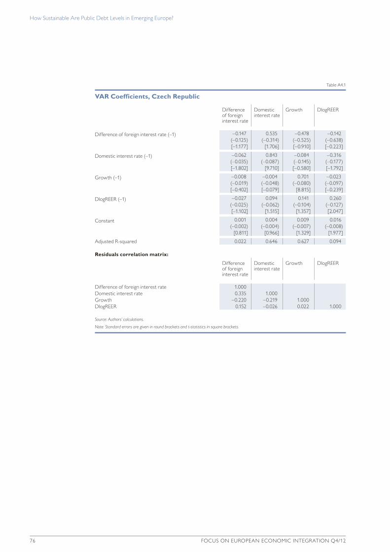
How Sustainable are public Debt Levels in emerging europe?
76 FocuS on european economic integration Q4/12
table a4.1
VAR Coefficients, Czech Republic
Difference of foreign interest rate
Domestic interest rate
growth Dlogreer
Difference of foreign interest rate (–1) –0.147 0.535 –0.478 –0.142 (–0.125) (–0.314) (–0.525) (–0.638) [–1.177] [1.706] [–0.910] [–0.223]
Domestic interest rate (–1) –0.062 0.843 –0.084 –0.316 (–0.035) (–0.087) (–0.145) (–0.177) [–1.802] [9.710] [–0.580] [–1.792]
growth (–1) –0.008 –0.004 0.701 –0.023 (–0.019) (–0.048) (–0.080) (–0.097) [–0.402] [–0.079] [8.815] [–0.239]
Dlogreer (–1) –0.027 0.094 0.141 0.260 (–0.025) (–0.062) (–0.104) (–0.127) [–1.102] [1.515] [1.357] [2.047]
constant 0.001 0.004 0.009 0.016 (–0.002) (–0.004) (–0.007) (–0.008)
[0.811] [0.966] [1.329] [1.977]
adjusted r-squared 0.022 0.646 0.627 0.094
Residuals correlation matrix:
Difference of foreign interest rate
Domestic interest rate
growth Dlogreer
Difference of foreign interest rate 1.000Domestic interest rate 0.335 1.000growth –0.220 –0.219 1.000Dlogreer 0.152 –0.026 0.022 1.000
Source: Authors’ calculations.
Note: Standard errors are given in round brackets and t-statistics in square brackets.
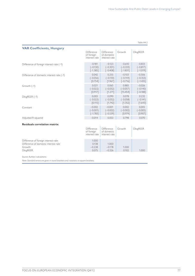
How Sustainable are public Debt Levels in emerging europe?
FocuS on european economic integration Q4/12 77
table a4.2
VAR Coefficients, HungaryDifference of foreign interest rate
Difference of domestic interest rate
growth Dlogreer
Difference of foreign interest rate (–1) –0.181 –0.123 –0.610 –0.833 (–0.130) (–0.301) (–0.333) (–0.817) [–1.385] [–0.408] [–1.831] [–1.019]
Difference of domestic interest rate (–1) 0.042 0.255 –0.103 –0.506 (–0.056) (–0.130) (–0.144) (–0.353)
[0.754] [1.967] [–0.716] [–1.435]
growth (–1) 0.021 0.065 0.883 –0.026 (–0.022) (–0.052) (–0.057) (–0.140)
[0.917] [1.271] [15.454] [–0.188]
Dlogreer (–1) 0.003 0.090 0.078 0.232 (–0.023) (–0.052) (–0.058) (–0.141)
[0.115] [1.742] [1.352] [1.643]
constant –0.002 –0.001 0.002 0.005 (–0.001) (–0.002) (–0.002) (–0.005) [–1.783] [–0.539] [0.974] [0.907]
adjusted r-squared –0.014 0.053 0.798 0.070
Residuals correlation matrix:
Difference of foreign interest rate
Difference of domestic interest rate
growth Dlogreer
Difference of foreign interest rate 1.000Difference of domestic interest rate 0.138 1.000growth –0.238 –0.178 1.000Dlogreer 0.075 –0.326 0.102 1.000
Source: Authors’ calculations.
Note: Standard errors are given in round brackets and t-statistics in square brackets.

How Sustainable are public Debt Levels in emerging europe?
78 FocuS on european economic integration Q4/12
table a4.3
VAR Coefficients, Poland
Difference of foreign interest rate
Domestic interest rate
growth Dlogreer
Difference of foreign interest rate (–1)
–0.154 –0.224 –0.188 –2.987 (–0.131) (–0.253) (–0.442) (–1.036) [–1.173] [–0.885] [–0.425] [–2.883]
Domestic interest rate (–1)
–0.014 0.806 –0.079 –0.146 (–0.039) (–0.074) (–0.130) (–0.305) [–0.359] [10.827] [–0.605] [–0.478]
growth (–1)
–0.022 –0.103 0.596 0.309 (–0.032) (–0.062) (–0.109) (–0.256) [–0.689] [–1.651] [5.457] [1.205]
Dlogreer (–1)
0.008 0.072 0.028 0.180 (–0.015) (–0.030) (–0.052) (–0.122)
[0.528] [2.423] [0.546] [1.478]
constant
0.000 0.011 0.020 –0.009 (–0.002) (–0.005) (–0.008) (–0.019)
[0.196] [2.305] [2.439] [–0.490]
adjusted r-squared –0.029 0.721 0.389 0.138
Residuals correlation matrix:
Difference of foreign interest rate
Domestic interest rate
growth Dlogreer
Difference of foreign interest rate 1.000Domestic interest rate 0.211 1.000growth 0.142 –0.190 1.000Dlogreer 0.023 0.028 0.016 1.000
Source: Authors’ calculations.
Note: Standard errors are given in round brackets and t-statistics in square brackets.

How Sustainable are public Debt Levels in emerging europe?
FocuS on european economic integration Q4/12 79
table a4.4
VAR Coefficients, Slovakia
Difference of foreign interest rate
Domestic interest rate
growth Dlogreer
Difference of foreign interest rate (–1) –0.189 1.085 –0.546 0.047 (–0.125) (–0.531) (–0.789) (–0.551) [–1.513] [2.043] [–0.693] [0.085]
Domestic interest rate (–1) 0.004 0.915 –0.081 –0.085 (–0.012) (–0.052) (–0.077) (–0.053)
[0.369] [17.754] [–1.056] [–1.585]
growth (–1) 0.001 0.066 0.629 0.131 (–0.015) (–0.065) (–0.096) (–0.067)
[0.060] [1.026] [6.568] [1.954]
Dlogreer (–1) 0.055 0.037 –0.152 0.220 (–0.028) (–0.118) (–0.176) (–0.123)
[1.973] [0.316] [–0.865] [1.787]
constant –0.002 0.001 0.020 0.005 (–0.001) (–0.005) (–0.007) (–0.005) [–1.680] [0.119] [2.857] [1.140]
adjusted r-squared 0.024 0.838 0.406 0.106
Residuals correlation matrix:
Difference of foreign interest rate
Domestic interest rate
growth Dlogreer
Difference of foreign interest rate 1.000Domestic interest rate –0.008 1.000growth –0.185 0.228 1.000Dlogreer 0.086 –0.181 –0.268 1.000
Source: Authors’ calculations.
Note: Standard errors are given in round brackets and t-statistics in square brackets.
table a5
Average Size of Simulations of the VAR Model and of the Fiscal Reaction Function
Foreign real interest rate
Domestic real interest rate
gDp growth rate of appreciation of the real effective exchange rate
primary balance
% p.a. % p.a. % year on year % year on year % of GDP
czech republic 0.03 1.90 2.71 1.26 –2.19(1.17) (1.87) (2.60) (1.69) (1.82)
Hungary –0.37 1.67 2.78 0.75 0.97(1.13) (4.06) (2.64) (1.71) (2.60)
poland –0.77 2.94 4.31 0.21 0.11(1.34) (1.62) (1.75) (2.60) (1.36)
Slovakia –0.99 2.01 4.50 1.19 –1.82(1.37) (4.27) (3.18) (1.39) (2.86)
Source: Authors’ calculations, Eurostat.
Note: Simulations are obtained by using equation (4.1) for the primary balance and (5.1) for all other variables. A positive value of the rate of appreciation of the exchange rate denotes appreciation. Standard deviations are given in percentage points in parentheses.