How Many Tiers? Pricing in the Internet Transit Market

Vytautas Valancius∗, Cristian Lumezanu∗, Nick Feamster∗,Ramesh Johari†, and Vijay V. Vazirani∗

∗ Georgia Tech † Stanford University

ABSTRACT

ISPs are increasingly selling “tiered” contracts, which offer Inter-net connectivity to wholesale customers in bundles, at rates basedon the cost of the links that the traffic in the bundle is traversing.Although providers have already begun to implement and deploytiered pricing contracts, little is known about how to structure them.Although contracts that sell connectivity on finer granularities im-prove market efficiency, they are also more costly for ISPs to im-plement and more difficult for customers to understand. Our goalis to analyze whether current tiered pricing practices in the whole-sale transit market yield optimal profits for ISPs and whether betterbundling strategies might exist. In the process, we offer two contri-butions: (1) we develop a novel way of mapping traffic and topol-ogy data to a demand and cost model; and (2) we fit this model onthree large real-world networks: an European transit ISP, a contentdistribution network, and an academic research network, and runcounterfactuals to evaluate the effects of different bundling strate-gies. Our results show that the common ISP practice of structuringtiered contracts according to the cost of carrying the traffic flows(e.g., offering a discount for traffic that is local) can be suboptimaland that dividing contracts based on both traffic demand and the

cost of carrying it into only three or four tiers yields near-optimalprofit for the ISP.

Categories and Subject Descriptors

C.2.3 [Network Operations]: Network Management

General Terms

Algorithms, Design, Economics

1. INTRODUCTIONThe increasing commoditization of Internet transit is changing

the landscape of the Internet bandwidth market. Although residen-tial Internet Service Providers (ISPs) and content providers are con-necting directly to one another more often, they must still use majorInternet transit providers to reach most destinations. These Internettransit customers can often select from among dozens of possibleproviders [26]. As major ISPs compete with one another, the priceof Internet transit continues to plummet: on average, transit pricesare falling by about 30% per year [22].

As a result of such competition, ISPs are evolving their businessmodels and selling transit to their customers in many ways to try

Permission to make digital or hard copies of all or part of this work forpersonal or classroom use is granted without fee provided that copies arenot made or distributed for profit or commercial advantage and that copiesbear this notice and the full citation on the first page. To copy otherwise, torepublish, to post on servers or to redistribute to lists, requires prior specificpermission and/or a fee.SIGCOMM’11, August 15–19, 2011, Toronto, Ontario, Canada.Copyright 2011 ACM 978-1-4503-0797-0/11/08 ...$10.00.

to retain profits. In particular, many transit ISPs implement pric-ing strategies where traffic is priced by volume or destination [8].For example, most transit ISPs offer volume discounts for highercommit levels (e.g., customer networks committing to a lower mini-mum bandwidth receive a higher per-bit price quote than customerscommitting to a higher minimum bandwidth [22]). Such a marketis said to implement tiered pricing [12]. Through private communi-cation with network operators, we identified many other instancesof tiered pricing already being implemented by ISPs. These pricinginstruments involve charging prices on traffic bundles based on var-ious factors, such as how far the traffic is traveling, and whether thetraffic is “on net” (i.e., to that ISP’s customers) or “off net”. Still,we understand very little about the extent to which tiered pricingbenefits both ISPs and their customers, or if there might be betterways to structure the tiers. In this paper, we study destination-

based tiered pricing, with the goal of understanding how ISPsshould bundle and price connectivity to maximize their profit.

In this study, we grapple with the balance between the prescrip-tions of economic theory and a variety of practical constraints andrealities. On one hand, economic theory says that higher marketgranularity leads to increased efficiency [16]. Intuitively, an In-ternet transit market that prices individual flows is more efficientthan one that sells transit in bulk, since customers pay only for thetraffic they send, and since ISPs can price those flows accordingto their cost. On the other hand, various practical constraints pre-vent Internet transit from being sold in arbitrarily fine granularities.Technical hurdles and additional overhead can make it difficult toimplement tiered pricing in current routing protocols and equip-ment. Additionally, tiered pricing can be more difficult for whole-sale customers to understand if there are too many tiers. TransitISPs would ideally like to come close to maximizing their profitwith only a few pricing tiers, since implementing more pricing tiersintroduces additional overhead and complexity. Our analysis showsthat, indeed, in many cases, an ISP reaps most of the profit possiblewith infinitesimally fine-grained tiers using only two or three tiers,assuming that those two or three tiers are structured properly.

Although understanding the benefits of different pricing struc-tures is important, modeling them is quite difficult. The modelmust take as an input existing customer demand and predict howtraffic (and, hence, ISP profit) would change in response to pric-ing strategies. Such a model must capture how customers wouldrespond to any pricing change—for any particular traffic flow—aswell as the change in cost of forwarding traffic on various paths inan ISP’s network. Of course, many of these input values are diffi-cult to come by even for network operators, but they are especiallyelusive for researchers; additionally, even if certain values such ascosts are known, they change quickly and differ widely across ISPs.

The model we develop allows us to estimate the relative effectsof pricing and bundling scenarios, despite the lack of availability ofprecise values for many of these parameters. The general approach,which we describe in Section 3, is to start with a demand and costmodel and assume both that ISPs are already profit-maximizing and

that the current prices reflects both customer demand and the un-derlying network costs. These assumptions allow us to either fix orsolve for many of the unknown parameters and run counterfactu-als to evaluate the relative effects of dividing the customer demandinto pricing tiers. To drive this model, we use traffic data from threereal-world networks: a major international content distribution net-work with its own network infrastructure; an European transit ISP;and an academic research network. We map the demand and topol-ogy data from these networks to a model that reflects the serviceofferings that real-world ISPs use.

Using our model, we evaluate three scenarios:

• What happens if an ISP increases the number of tiers for

which it sells transit? We find that profit increases, but thereturns diminish as the number of tiers increases: with 3–4 tiers, it is possible to capture 90–95% of the profit thatcould be captured with an infinite number of granularities,assuming that these tiers are divided in the right way.

• How do strategies for dividing capacity into distinct bundles

and pricing those bundles affect an ISP’s profit? Our analy-sis shows that ISPs must judiciously choose how they dividetraffic into pricing tiers. A naïve approach (e.g., based onlyon traffic cost or on demand) might require dozens of pric-ing tiers to capture most of the possible profit. We find thatdividing traffic into tiers in a way that accounts for both traf-

fic demand and the cost of carrying traffic yields more profitthan the current practice that is based only on cost, and isnearly as effective as an optimal division.

• How do the benefits of various pricing strategies depend on

the network topology and traffic demands? We find that net-works with high variability in cost of delivering traffic obtaingreater benefit from bundling. We also observe that networkswith high variability in demand require more bundles to cap-ture maximum profit.

We evaluate these and other questions across two customer demandmodels, four network cost models, and a range of input parameters,such as price sensitivity. Although each of the models might not beperfectly accurate, they yield results that are consistent both acrossmodels and with our intuition about markets.

We make three contributions. First, we taxonomize the state ofthe art and trends in pricing instruments for Internet transit (Sec-tion 2). Second, to analyze the effects of tiered pricing, we developa model that captures demands and costs in the transit market. Oneof the challenges in developing such a model is applying it to realtraffic data, given many unknown parameters (e.g., the cost of var-ious resources, or how users respond to price). Hence, we developmethods for fitting empirical traffic demands to theoretical cost anddemand models. We use this approach to evaluate ISP profit forpricing strategies under a range of possible cost models and net-work topologies (Section 3). Third, we apply our model to real-world traffic matrices and characterize a range of simple bundlingstrategies that are close to optimal (Section 4); we also suggest howthese strategies could be implemented in practice (Section 5).

2. BACKGROUNDIn this section, we describe the current state of affairs in the In-

ternet transit market. We first taxonomize what services (bundles)ISPs are selling. We then provide intuition on why ISPs are movingtowards tiered wholesale Internet transit service.

2.1 Current Transit Market OfferingsUnfortunately, there is not much public information about the

wholesale Internet transit market. ISPs are reluctant to reveal

specifics about their business models and pricing strategies to theircompetitors. Therefore, to obtain most of the information in thissection, we engaged in many discussions and email exchanges withnetwork operators. Below, we classify the types of Internet transitservice we identified during these conversations. Although muchof the information in this section is widely known in the networkoperations community, it is difficult to find a concise taxonomy ofproduct offerings in the wholesale transit market. The taxonomybelow serves as a point of reference for our discussions of tieredpricing in this paper, but it may also be useful for anyone whowishes to better understand the state of the art in pricing strategiesin the wholesale transit market.

Transit. Most ISPs offer conventional Internet transit service. In-ternet transit is sold at a blended rate—a single price (usuallyexpressed in $/Mbps/month)—charged for traffic to all destina-tions. Historically, blended rates have been decreasing by 30%each year [22]. Blended rate is the simplest and yet the most crudeway to charge for traffic. If network costs are highly variable, lesscostly flows in the blended-rate bundle subsidize other, more ex-pensive flows. ISPs often innovate by offering more than one rate:We summarize three pricing models that require two or more rates:(1) paid peering, (2) backplane peering, and (3) regional pricing.

Paid peering is similar to settlement-free peering, except that onenetwork pays to reach the other. A major ISP might separatelysell off-net routes (wholesale transit) at one rate and on-net routes(to reach destinations inside its own network) at another (usuallylower) rate. For example, national ISPs in Eastern Europe, Aus-tralia, and in other regions may sell local connectivity at a dis-count to increase demand for local traffic, which is is significantlycheaper than transit to outside global destinations [1]. The on-netroutes are also offered at a discount by some major transit ISPsto large content providers, because such transit ISPs can recouppart of the costs from their customers, who congest paid upstreamlinks to transit ISPs by downloading the content. Some instances ofpaid peering have spawned significant controversy: most recently,Comcast—primarily a network serving end-users—was accused ofa network neutrality violation when it forced one tier-1 provider topay to reach Comcast’s customers [15].

Backplane peering occurs when an ISP, in addition to sellingglobal transit through its own backbone, charges a discount rate forthe traffic it can offload to its peers at the same Internet exchange.Smaller ISPs buy such a service because they might not meet allthe settlement-free peering requirements to peer directly with theISPs in the exchange. Although many large ISPs discourage thispractice, some ISPs deviate by offering backplane peering to retaincustomers or to maintain traffic ratios with their peers. As withpaid peering, the ISP selling backplane peering has to account andcharge for at least two traffic flows: one to peers and another to itsbackbone.

Regional pricing occurs when transit service providers offer differ-ent rates to reach different geographic regions. The regions can bedefined at different levels of granularity, such as PoP, metro area,regional area, nation, or continent. In some instances, the tran-sit ISP offers access to all regions with different prices; in otherinstances, the downstream network purchases access only to a spe-cific geographic region (e.g., access only to South America or Aus-tralia). In practice, due to the overhead of provisioning and main-taining many sessions to the same customer, ISPs rarely use morethan one or two extra price levels for different regions.

We speculate that the bundling strategies described above aroseprimarily from operational and cost considerations. For example,it is relatively easy for a transit ISP to tag which routes are coming

0 Q1 1 2 Q2 3 4 5 6Quantity (Mbps)

0

0.5

1.0P ∗

1.5

2.0

2.5

3.0

Unit

pri

ce (

$/M

bps)

Demand D2

Demand D1

Surplus = $4.17

Revenue (Profit = $2.08)

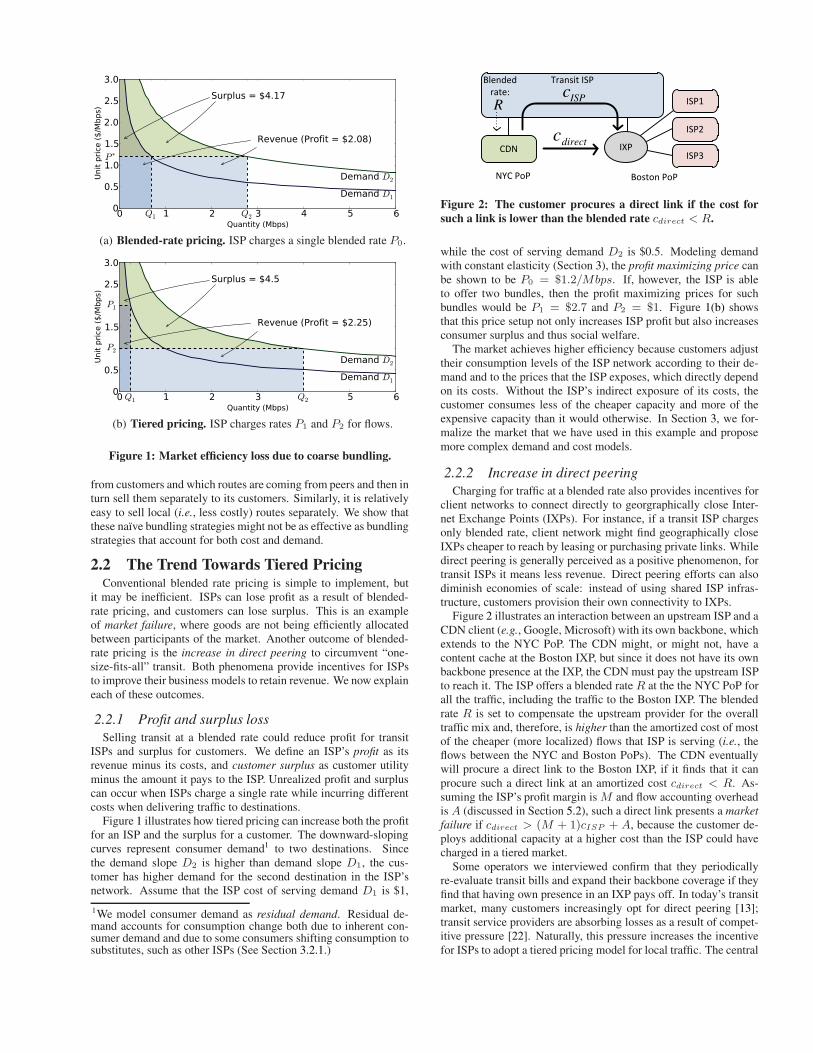
(a) Blended-rate pricing. ISP charges a single blended rate P0.

0 Q1 1 2 3 Q2 5 6Quantity (Mbps)

0

0.5

P2

1.5

P1

2.5

3.0

Unit

pri

ce (

$/M

bps)

Demand D2

Demand D1

Surplus = $4.5

Revenue (Profit = $2.25)

(b) Tiered pricing. ISP charges rates P1 and P2 for flows.

Figure 1: Market efficiency loss due to coarse bundling.

from customers and which routes are coming from peers and then inturn sell them separately to its customers. Similarly, it is relativelyeasy to sell local (i.e., less costly) routes separately. We show thatthese naïve bundling strategies might not be as effective as bundlingstrategies that account for both cost and demand.

2.2 The Trend Towards Tiered PricingConventional blended rate pricing is simple to implement, but

it may be inefficient. ISPs can lose profit as a result of blended-rate pricing, and customers can lose surplus. This is an exampleof market failure, where goods are not being efficiently allocatedbetween participants of the market. Another outcome of blended-rate pricing is the increase in direct peering to circumvent “one-size-fits-all” transit. Both phenomena provide incentives for ISPsto improve their business models to retain revenue. We now explaineach of these outcomes.

2.2.1 Profit and surplus loss

Selling transit at a blended rate could reduce profit for transitISPs and surplus for customers. We define an ISP’s profit as itsrevenue minus its costs, and customer surplus as customer utilityminus the amount it pays to the ISP. Unrealized profit and surpluscan occur when ISPs charge a single rate while incurring differentcosts when delivering traffic to destinations.

Figure 1 illustrates how tiered pricing can increase both the profitfor an ISP and the surplus for a customer. The downward-slopingcurves represent consumer demand1 to two destinations. Sincethe demand slope D2 is higher than demand slope D1, the cus-tomer has higher demand for the second destination in the ISP’snetwork. Assume that the ISP cost of serving demand D1 is $1,

1We model consumer demand as residual demand. Residual de-mand accounts for consumption change both due to inherent con-sumer demand and due to some consumers shifting consumption tosubstitutes, such as other ISPs (See Section 3.2.1.)

Transit ISP

CDN

ISP1

ISP2

ISP3IXP

NYC PoP Boston PoP

ISPc

directc

R

Blended

rate:

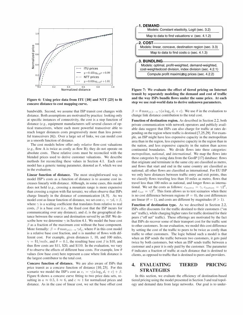
Figure 2: The customer procures a direct link if the cost for

such a link is lower than the blended rate cdirect < R.

while the cost of serving demand D2 is $0.5. Modeling demandwith constant elasticity (Section 3), the profit maximizing price canbe shown to be P0 = $1.2/Mbps. If, however, the ISP is ableto offer two bundles, then the profit maximizing prices for suchbundles would be P1 = $2.7 and P2 = $1. Figure 1(b) showsthat this price setup not only increases ISP profit but also increasesconsumer surplus and thus social welfare.

The market achieves higher efficiency because customers adjusttheir consumption levels of the ISP network according to their de-mand and to the prices that the ISP exposes, which directly dependon its costs. Without the ISP’s indirect exposure of its costs, thecustomer consumes less of the cheaper capacity and more of theexpensive capacity than it would otherwise. In Section 3, we for-malize the market that we have used in this example and proposemore complex demand and cost models.

2.2.2 Increase in direct peering

Charging for traffic at a blended rate also provides incentives forclient networks to connect directly to georgraphically close Inter-net Exchange Points (IXPs). For instance, if a transit ISP chargesonly blended rate, client network might find geographically closeIXPs cheaper to reach by leasing or purchasing private links. Whiledirect peering is generally perceived as a positive phenomenon, fortransit ISPs it means less revenue. Direct peering efforts can alsodiminish economies of scale: instead of using shared ISP infras-tructure, customers provision their own connectivity to IXPs.

Figure 2 illustrates an interaction between an upstream ISP and aCDN client (e.g., Google, Microsoft) with its own backbone, whichextends to the NYC PoP. The CDN might, or might not, have acontent cache at the Boston IXP, but since it does not have its ownbackbone presence at the IXP, the CDN must pay the upstream ISPto reach it. The ISP offers a blended rate R at the the NYC PoP forall the traffic, including the traffic to the Boston IXP. The blendedrate R is set to compensate the upstream provider for the overalltraffic mix and, therefore, is higher than the amortized cost of mostof the cheaper (more localized) flows that ISP is serving (i.e., theflows between the NYC and Boston PoPs). The CDN eventuallywill procure a direct link to the Boston IXP, if it finds that it canprocure such a direct link at an amortized cost cdirect < R. As-suming the ISP’s profit margin is M and flow accounting overheadis A (discussed in Section 5.2), such a direct link presents a market

failure if cdirect > (M + 1)cISP + A, because the customer de-ploys additional capacity at a higher cost than the ISP could havecharged in a tiered market.

Some operators we interviewed confirm that they periodicallyre-evaluate transit bills and expand their backbone coverage if theyfind that having own presence in an IXP pays off. In today’s transitmarket, many customers increasingly opt for direct peering [13];transit service providers are absorbing losses as a result of compet-itive pressure [22]. Naturally, this pressure increases the incentivefor ISPs to adopt a tiered pricing model for local traffic. The central

question, then, is how they should go about structuring these tiers.The rest of the paper focuses on this question.

3. MODELING PROFITS, COSTS, AND

DEMANDSWe develop demand and cost models that capture ISP profit un-

der various pricing strategies. Although we doubt there is a perfectmodel for demand in the Internet transit market, we perform ourevaluation with two common demand models. Because cost is alsodifficult to model, we devise four network cost models. We firstdefine ISP profit and then describe demand and cost models.

3.1 ISP ProfitWe consider a transit market with multiple ISPs and customers.

Each ISP is rational and maximizes its profit, which we express asthe difference between its revenue and costs:

Π(~P ) =∑

pi∈~P

(

piQi(~P )− ciQi(~P ))

(1)

where pi is the price an ISP sets to deliver flow i, ci is the unit

cost for i, and Qi(~P ) is the demand for i given a vector of prices~P = (p1, p2, . . . , pn). An ISP chooses the price vector ~P thatmaximizes its profit. Having a price for each flow allows us toexplore different pricing strategies by bundling flows in differentways. For example, blended rate pricing requires pi to be equal forall i; we can explore different tiered pricing approaches by requir-ing various subsets of all flows to have the same price.

Given knowledge of both the traffic demand of customers andthe costs associated with delivering each flow, we can compute ISPprofit. Unfortunately, it is difficult to validate any particular de-mand function or cost model; even if validation were possible, itis likely that cost structures and customer demand could change orevolve over time. Accordingly, we evaluate ISP profit for varioustiered pricing approaches under a variety of demand functions andcost models. Section 3.2 describes the demand functions that weexplore, and Section 3.3 describes the cost models that we consider.

3.2 Customer DemandTo compute ISP profit for each pricing scenario, we must under-

stand how customers adjust their traffic demand in response to pricechanges. We consider two families of demand functions: constant

elasticity and logit.

Constant elasticity demand. The constant elasticity de-mand (CED) is derived from the well-known alpha-fair utilitymodel [20], which is often used to model user utility on the In-ternet. The alpha-fair utility takes the form of a concave increasingutility function, which emulates a decreasing marginal benefit toadditional bandwidth for a user. In this model flow demands areseparable (i.e., changes in demand or prices for one flow have noeffect on demand and prices of other flows). The CED model ismost appropriate for scenarios when consumers have no alterna-tives (e.g., when the content that a customer is trying to reach is notreplicated, or the customer needs to communicate with a specificendpoint on the network).

Logit demand. To capture the fact that customers might some-times have a choice between flows (e.g., sending traffic to alterna-tive destination if the current one becomes too expensive), we alsoperform our analysis using the logit model, where demands are notseparable: the price and demand for any flow depend on prices anddemands for the other flows. The logit model is frequently used forthis purpose in econometric demand estimation [18]. In the logit

0.0 0.5 1.0 1.5 2.0 2.5 3.0 3.5 4.0

Quantity (Mbps)

0.0

0.5

1.0

1.5

2.0

2.5

3.0

3.5

4.0

Pri

ce (

$)

Feasible demand space

α=3.3

α=1.4

Figure 3: Feasible CED demand functions.

1 p ∗

1 3 p ∗

2 5 6 7

Price ($)

0.00

0.05

0.10

0.15

0.20

0.25

Pro

fit

($)

c1 =$1.0

c2 =$2.0

Figure 4: Profit for two flows with identical demand (v1 = v2 =1.0, α = 2) but different cost.

model, each consumer nominally prefers the flows that offers thehighest utility. This matches well with scenarios when consumershave several alternatives (e.g., when requested content is replicatedin multiple places).

3.2.1 Constant elasticity demand

The CED demand function is as follows:

Qi(pi) =

(

vipi

)α

(2)

where pi is the unit price (e.g., $/Mbit/s), α ∈ (1,∞) is the pricesensitivity, and vi > 0 is the valuation coefficient of flow i. The de-mand function can be interpreted to represent either inherent con-sumer demand or residual consumer demand, which reflects notonly the inherent demand but also the availability of substitutes.

Figure 3 presents example CED demand functions for v = 1and two values of α, 3.3 and 1.4. Higher values of α indicate highelasticity (users reduce use even due to small changes in price).For example, the line labeled α = 3.3 might represent the trafficfrom residential ISPs, who are more sensitive to wholesale Inter-net prices and who respond to price changes in a more dramaticway. Although our model does not capture full dynamic interac-tion between competing ISPs (e.g., price wars), modeling demandas residual allows us to account for the existing competitive en-vironment and switching costs. As discussed above, high elastic-ity can also indicate that competitors are offering more affordablesubstitutes, and that switching costs for customers are low. In ourevaluation, we use a range of price sensitivity values to measurehow ISP profit changes for different values of the elasticity of userdemand. The gray area in Figure 3 shows that we can cover all fea-sible demand functions simply by varying the sensitivity parameter.

CED profit. Using the expressions for ISP profit (Equation 1) anddemand (Equation 2), and assuming separability of demand of dif-ferent flows, the ISP profit is:

Π(~P ) =∑

pi∈~P

(

vipi

)α

(pi − ci) . (3)

CED profit-maximizing price. By differentiating the profit, wefind the profit-maximizing price for each flow i:

p∗i =αciα− 1

. (4)

Figure 4 illustrates profit maximization for two flows that haveidentical demand functions but different costs. For example, thefirst flow costs c1 = $1.0 per unit to deliver and mandates optimalprice p∗ = $2.0 which results in $0.25 profit. The second flow ismore costly thus the profit maximizing price is higher. In this case,the first plot might represent profit for local traffic, while the sec-ond plot represents national traffic: ISPs must price national traffichigher than local-area traffic to maximize profit.

CED price for bundled flows. In our evaluation, we test variouspricing strategies that bundle multiple flows under the same profit-maximizing price. To find the price for each bundle, we first mapreal world demands to our model to obtain the valuation vi andcost ci for each flow. Then, we differentiate the profit (Equation 3)with respect to the price of each bundle. For example, when wehave a single bundle for all flows, we obtain the following profit-maximizing price:

P ∗ =α∑n

i=1 civαi

(α− 1)∑n

i=1 vαi

(5)

where n is the number of flows. Section 4 details this approach.

3.2.2 Logit demand

The logit demand model assumes that each consumer faces adiscrete choice among a set of available goods or services. In thecontext of data transit, the choice is between different destinationsor flows. Following Besanko et al. [?], a consumer j using flow iwill obtain the utility:

uij = α(vi − pi) + ǫij

where α ∈ (0,∞) is the elasticity parameter, vi is the “average”consumer’s maximum willingness to pay for flow i, pi is a priceof using i, and ǫij represents consumer j’s idiosyncratic preferencefor i (where ǫij has a Gumbel distribution.) The logit model definesthe probability that any given consumer will use flow i as a functionof the price vector of all flows:

si(~P ) =eα(vi−pi)

∑

j eα(vj−pj) + 1

(6)

where∑

i si(~P ) = 1. The demand for flow i equals the product of

si(~P ) and the total number of consumers (K):

Qi(~P ) = Ksi(~P ). (7)

Here, si is also called the market share of flow i. The model alsoaccounts for the possibility that some customers elect not to sendtraffic to any destination. The market share for traffic not sent is:

s0(~P ) =1

∑

j eα(vj−pj) + 1

.

0.0 0.2 0.4 0.6 0.8 1.0

Quantity

0.0

0.5

1.0

1.5

2.0

2.5

3.0

3.5

4.0

Pri

ce

Feasible demand space

α=1

α=2

Figure 5: Logit demand function.

Figure 5 shows examples of logit demand functions. We assumea setting with two flows, with two values for the valuation vi, 1.6and 1. We fix the price for the first flow to 1, and we vary the pricefor the second flow between 0 and 4. The figure shows demandcurves for the second flow, for two values of α. Similar to theconstant elasticity demand model, lower values of α indicate lowelasticity of demand, where users need bigger price variations tomodify their usage.

Logit profit. Using the expressions for ISP profit (Equation 1) andlogit demand (Equation 7), the ISP profit is:

Π(~P ) = K∑

pi∈~P

si(~P )(pi − ci). (8)

Logit profit-maximizing prices. To find the profit maximizingprice for flow i, we differentiate the profit with respect to price pi:

p∗i = ci +1

αs0. (9)

Due to the presence of s0, p∗i recursively depends on itself and onprofit-maximizing prices of other flows. To obtain maximum profit,we develop a heuristic based on gradient descent that starts from afixed set of prices and greedily updates them towards the optimum.

Valuation and cost of bundled flows. To test pricing strategies, wefirst map real traffic demands to the model to find the valuation viand cost ci for each flow i. We then bundle the flows as describedin Section 4.2.1. Knowing that

∑

i si = 1 and applying Equation 6allows us to compute valuations for any bundle of flows as:

vbundle =ln

(∑n

i=1 eαvi

)

α(10)

where vi are valuations of the flows in the bundle. Similarly we canfind the average unit cost of combined flows in each bundle:

cbundle =

∑n

i=1 cieαvi

∑n

i=1 eαvi

. (11)

3.3 ISP CostModeling cost is difficult: ISPs typically do not publish the de-

tails of operational costs; even if they did, many of these figureschange rapidly and are specific to the ISP, the region, and otherfactors. To account for these uncertainties, we evaluate our resultsin the context of several cost models. We also make the follow-ing assumptions. First, we assume the more traffic the ISP car-ries, the higher cost it incurs. Although on a small scale the band-width cost is a step function (the capacity is added at discrete in-crements), on a larger scale we model cost as a linear function of

0.0 0.2 0.4 0.6 0.8 1.0

Normalized distance

0.0

0.2

0.4

0.6

0.8

1.0N

orm

alized p

rice

ITU prices

y=0.43log9.43x+0.99

NTT prices

y=0.03log1.12x+1.01

Figure 6: Using price data from ITU [10] and NTT [23] to fit

concave distance to cost mapping curve.

bandwidth. Second, we assume that ISP transit cost changes withdistance. Both assumptions are motivated by practice: looking onlyat specific instances of connectivity, the cost is a step function ofdistance (e.g., equipment manufacturers sell several classes of op-tical transceivers, where each more powerful transceiver able toreach longer distances costs progressively more than less power-ful transceivers [6]). Over a large set of links, we can model costas a smooth function of distance.

The cost models below offer only relative flow-cost valuations(e.g., flow A is twice as costly as flow B); they do not operate onabsolute costs. These relative costs must be reconciled with theblended prices used to derive customer valuations. We describemethods for reconciling these values in Section 4.1. Each costmodel has a generic tuning parameter, denoted as θ, which we usein the evaluation.

Linear function of distance. The most straightforward way tomodel ISP’s costs as a function of distance is to assume cost in-creases linearly with distance. Although, in some cases, this modeldoes not hold (e.g., crossing a mountain range is more expensivethan crossing a region with flat terrain), we often observe that ISPscharge linearly in the distance of communication [4, 5]. As wemodel cost as linear function of distance, we set cost ci = γdi+β,where γ is a scaling coefficient that translates from relative to realcosts, β is a base cost (i.e., the fixed cost that the ISP incurs forcommunicating over any distance), and di is the geographical dis-tance between the source and destination served by an ISP. We de-scribe how we determine γ in Section 4.1. We model the base costβ as a fraction of the maximum cost without the base component.More formally: β = θmaxj∈1···n γdj , where θ in this cost modelis a relative base cost fraction, and n is number of flows with dif-ferent cost. For example, given distances 1, 10, and 100 miles,γ = $1/mile, and θ = 0.1, the resulting base cost β is $10, andthus flow costs are $11, $20, and $110. In the evaluation, we varyθ to observe the effects of different base costs. For example, low θvalues (low base cost) here represent a case where link distance isthe largest contributor to the total cost.

Concave function of distance. We are also aware of ISPs thatprice transit as a concave function of distance [10, 23]. For thisscenario we model the ISP’s cost as ci = γ(a logb di + c) + β.Figure 6 shows a concave curve fitting to two price data sets, re-sulting in a ≈ 0.5, b ≈ 6, and c ≈ 1 for normalized prices anddistance. As in the case of linear cost, we set the base offset cost

2. COST

Models: linear, concave, destination region (sec. 3.3)

Map to data to find costs ci (sec. 4.1.3)

1. DEMAND

Models: Constant elasticity, Logit (sec. 3.2)

Map to data to find valuations vi (sec. 4.1.2)

3. BUNDLING

Models: optimal, profit@weighted, demand@weighted, cost@weightedcost division, index division (sec. 4.2.1)

Compute profit maximizing prices (sec. 4.2.2)

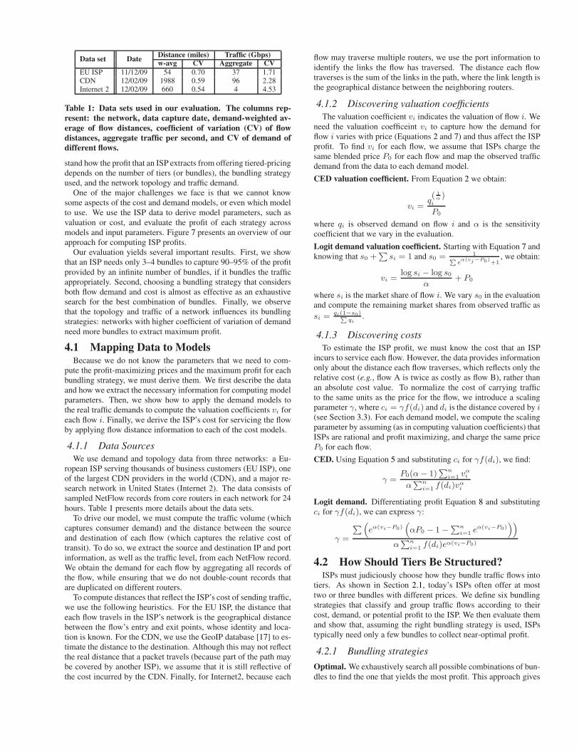
Figure 7: We evaluate the effect of tiered pricing on Internet

transit by separately modeling the demand and cost of traffic

and the way ISPs bundle flows under the same price. At each

step we use real-world data to derive unknown parameters.

β = θmaxj∈1···n γ(a logb di + c). We use θ in the evaluation tochange link distance contribution to the total cost.

Function of destination region. As described in Section 2.2, bothprivate communication with network operators and publicly avail-able data suggest that ISPs can also charge for traffic at rates de-pending on the region where traffic is destined [7,25,29]. For exam-ple, an ISP might have less expensive capacity in the metropolitanarea than in the region, less expensive capacity in the region than inthe nation, and less expensive capacity in the nation than acrosscontinental boundaries. We divide flows into three categories:metropolitan, national, and international. We map the flows intothese categories by using data from the GeoIP [17] database: flowsthat originate and terminate in the same city are classified as metro,and flows that start and end in the same country are classified asnational; all other flows are classified as international. For EU ISPwe only have distances between traffic entry and exit points, thuswe classify flows traveling less than 10 miles as metro, flows thattravel less than 100 miles as national, and longer flows as interna-tional. We set the costs as follows: cmetro = γ, cnation = γ2θ ,and cint = γ3θ . This form allows us to test scenarios when thereis no cost difference between regions (θ = 0), the cost differencesare linear (θ = 1), and costs are different by magnitudes (θ > 1).

Function of destination type. As we described in Section 2.2,ISPs offer discounts for the traffic destined to their customers (“onnet” traffic), while charging higher rates for traffic destined for theirpeers (“off net” traffic). These offerings are motivated by the factthat ISPs do recover some of their transport cost for the traffic sentto other customers. In our evaluation, we model this cost differenceby setting the cost of the traffic to peers to be twice as costly thantraffic to other customers. The logic behind such a model is thatwhen an ISP sends the traffic between two customers, it gets paidtwice by both customers, but when an ISP sends traffic between acustomer and a peer it is only paid by the customer. The parameterθ indicates a fraction of traffic at each distance that is destined toclients, as opposed to traffic that is destined to peers and providers.

4. EVALUATING TIERED PRICING

STRATEGIESIn this section, we evaluate the efficiency of destination-based

tiered pricing using the model presented in Section 3 and real topol-ogy and demand data from large networks. Our goal is to under-

Data set DateDistance (miles) Traffic (Gbps)w-avg CV Aggregate CV

EU ISP 11/12/09 54 0.70 37 1.71CDN 12/02/09 1988 0.59 96 2.28Internet 2 12/02/09 660 0.54 4 4.53

Table 1: Data sets used in our evaluation. The columns rep-

resent: the network, data capture date, demand-weighted av-

erage of flow distances, coefficient of variation (CV) of flow

distances, aggregate traffic per second, and CV of demand of

different flows.

stand how the profit that an ISP extracts from offering tiered-pricingdepends on the number of tiers (or bundles), the bundling strategyused, and the network topology and traffic demand.

One of the major challenges we face is that we cannot knowsome aspects of the cost and demand models, or even which modelto use. We use the ISP data to derive model parameters, such asvaluation or cost, and evaluate the profit of each strategy acrossmodels and input parameters. Figure 7 presents an overview of ourapproach for computing ISP profits.

Our evaluation yields several important results. First, we showthat an ISP needs only 3–4 bundles to capture 90–95% of the profitprovided by an infinite number of bundles, if it bundles the trafficappropriately. Second, choosing a bundling strategy that considersboth flow demand and cost is almost as effective as an exhaustivesearch for the best combination of bundles. Finally, we observethat the topology and traffic of a network influences its bundlingstrategies: networks with higher coefficient of variation of demandneed more bundles to extract maximum profit.

4.1 Mapping Data to ModelsBecause we do not know the parameters that we need to com-

pute the profit-maximizing prices and the maximum profit for eachbundling strategy, we must derive them. We first describe the dataand how we extract the necessary information for computing modelparameters. Then, we show how to apply the demand models tothe real traffic demands to compute the valuation coefficients vi foreach flow i. Finally, we derive the ISP’s cost for servicing the flowby applying flow distance information to each of the cost models.

4.1.1 Data Sources

We use demand and topology data from three networks: a Eu-ropean ISP serving thousands of business customers (EU ISP), oneof the largest CDN providers in the world (CDN), and a major re-search network in United States (Internet 2). The data consists ofsampled NetFlow records from core routers in each network for 24hours. Table 1 presents more details about the data sets.

To drive our model, we must compute the traffic volume (whichcaptures consumer demand) and the distance between the sourceand destination of each flow (which captures the relative cost oftransit). To do so, we extract the source and destination IP and portinformation, as well as the traffic level, from each NetFlow record.We obtain the demand for each flow by aggregating all records ofthe flow, while ensuring that we do not double-count records thatare duplicated on different routers.

To compute distances that reflect the ISP’s cost of sending traffic,we use the following heuristics. For the EU ISP, the distance thateach flow travels in the ISP’s network is the geographical distancebetween the flow’s entry and exit points, whose identity and loca-tion is known. For the CDN, we use the GeoIP database [17] to es-timate the distance to the destination. Although this may not reflectthe real distance that a packet travels (because part of the path maybe covered by another ISP), we assume that it is still reflective ofthe cost incurred by the CDN. Finally, for Internet2, because each

flow may traverse multiple routers, we use the port information toidentify the links the flow has traversed. The distance each flowtraverses is the sum of the links in the path, where the link length isthe geographical distance between the neighboring routers.

4.1.2 Discovering valuation coefficients

The valuation coefficient vi indicates the valuation of flow i. Weneed the valuation coefficeint vi to capture how the demand forflow i varies with price (Equations 2 and 7) and thus affect the ISPprofit. To find vi for each flow, we assume that ISPs charge thesame blended price P0 for each flow and map the observed trafficdemand from the data to each demand model.

CED valuation coefficient. From Equation 2 we obtain:

vi =q( 1α )

i

P0

where qi is observed demand on flow i and α is the sensitivitycoefficient that we vary in the evaluation.

Logit demand valuation coefficient. Starting with Equation 7 andknowing that s0 +

∑

si = 1 and s0 = 1∑

eα(vj−P0)

+1, we obtain:

vi =log si − log s0

α+ P0

where si is the market share of flow i. We vary s0 in the evaluationand compute the remaining market shares from observed traffic as

si =qi(1−s0)∑

qi.

4.1.3 Discovering costs

To estimate the ISP profit, we must know the cost that an ISPincurs to service each flow. However, the data provides informationonly about the distance each flow traverses, which reflects only therelative cost (e.g., flow A is twice as costly as flow B), rather thanan absolute cost value. To normalize the cost of carrying trafficto the same units as the price for the flow, we introduce a scalingparameter γ, where ci = γf(di) and di is the distance covered by i(see Section 3.3). For each demand model, we compute the scalingparameter by assuming (as in computing valuation coefficients) thatISPs are rational and profit maximizing, and charge the same priceP0 for each flow.

CED. Using Equation 5 and substituting ci for γf(di), we find:

γ =P0(α− 1)

∑n

i=1 vαi

α∑n

i=1 f(di)vαi

Logit demand. Differentiating profit Equation 8 and substitutingci for γf(di), we can express γ:

γ =

∑

(

eα(vi−P0)(

αP0 − 1−∑n

i=1 eα(vi−P0)

))

α∑n

i=1 f(di)eα(vi−P0)

4.2 How Should Tiers Be Structured?ISPs must judiciously choose how they bundle traffic flows into

tiers. As shown in Section 2.1, today’s ISPs often offer at mosttwo or three bundles with different prices. We define six bundlingstrategies that classify and group traffic flows according to theircost, demand, or potential profit to the ISP. We then evaluate themand show that, assuming the right bundling strategy is used, ISPstypically need only a few bundles to collect near-optimal profit.

4.2.1 Bundling strategies

Optimal. We exhaustively search all possible combinations of bun-dles to find the one that yields the most profit. This approach gives

1 2 3 4 5 6# of bundles

0.0

0.2

0.4

0.6

0.8

1.0Pr

ofit

cap

ture

OptimalCost-weightedProfit-weightedDemand-weightedCost divisionIndex division

(a) European ISP.

1 2 3 4 5 6# of bundles

0.0

0.2

0.4

0.6

0.8

1.0

Prof

it c

aptu

re

OptimalCost-weightedProfit-weightedDemand-weightedCost divisionIndex division

(b) Internet2.

1 2 3 4 5 6# of bundles

0.0

0.2

0.4

0.6

0.8

1.0

Prof

it c

aptu

re

OptimalCost-weightedProfit-weightedDemand-weightedCost divisionIndex division

(c) International CDN.

Figure 8: Profit capture for different bundling strategies in constant elasticity demand.

1 2 3 4 5 6# of bundles

0.0

0.2

0.4

0.6

0.8

1.0

Prof

it c

aptu

re

OptimalCost-weightedProfit-weightedCost divisionIndex division

(a) European ISP.

1 2 3 4 5 6# of bundles

0.0

0.2

0.4

0.6

0.8

1.0Pr

ofit

cap

ture

OptimalCost-weightedProfit-weightedCost divisionIndex division

(b) Internet2.

1 2 3 4 5 6# of bundles

0.0

0.2

0.4

0.6

0.8

1.0

Prof

it c

aptu

re

OptimalCost-weightedProfit-weightedCost divisionIndex division

(c) International CDN.

Figure 9: Profit capture for different bundling strategies in logit demand.

optimal results and also serves as our baseline against which wecompare other strategies. Computing the optimal bundling is com-putationally expensive: for example, there is more than a billionways to divide one hundred traffic flows into six pricing bundles.Presented below, all of the other bundling strategies employ heuris-tics to make bundling computationally tractable.

Demand-weighted. In this strategy, we use an algorithm inspiredby token buckets to group traffic flows to bundles. First, we set theoverall token budget as the sum of the original demand of all flows:T =

∑

i qi. Then, for each bundle j we assign the same tokenbudget tj = T/B, where B is the number of bundles we want tocreate. We sort the flows in decreasing order of their demand andtraverse them one-by-one. When traversing flow i, we assign it tothe first bundle j that either has no flows assigned to it or has abudget tj > 0. We reduce the budget of that bundle by qi. If theresulting budget tj < 0, we set tj+1 = tj+1 + tj . After traversingall the flows, the token budget of every bundle will be zero, andeach flow will be assigned to a bundle. The algorithm leads toseparate bundles for high demand flows and shared bundles for lowdemand flows. For example, if we need to divide four flows withdemands 30, 10, 10, and 10 into two bundles, the algorithm willplace the first flow in the first bundle, and the other three flows inthe second bundle.

Cost-weighted. We use the same approach as in demand-weightedbundling, but we set the token budget to T =

∑

i 1/ci. When plac-ing a flow in a bundle we remove a number of tokens equal to theinverse of its cost. This approach creates separate bundles for localflows and shared bundles for flows traversing longer distances. Thecurrent ISP practices of offering regional pricing and backplane

peering maps closely to using just two or three bundles arrangedusing this cost-weighted strategy.

Profit-weighted. The bundling algorithms described above con-sider cost and demand separately. To account for cost and demandtogether, we estimate potential profit each flow could bring. We usethe potential profit metric to apply the same weighting algorithm asin cost and demand-weighted bundling. In case of constant elastic-ity demand, we derive potential profit of each flow i:

πi =vαiα

(

αciα− 1

)1−α

(12)

For the logit demand, substituting pi in Equation 9 yields:

πi = Ksi(pi − ci) =Ksiαs0

∝ qi (13)

Cost division. We find the most expensive flow and divide thecost into ranges according to that value. For example, if wewant to introduce two bundles and the most expensive flow costs$10/Mbps/month to reach, we assign flows that cost $0–$4.99 tothe first bundle and flows that cost $5–$10 to the second bundle.

Index division. Index-division bundling is similar to cost divisionbundling, except that we rank flows according to their cost and usethe rank, rather than the cost, to perform the division into bundles.

4.2.2 The effects of different bundling strategies

To evaluate the bundling strategies described above, we com-pute the profit-maximizing prices and measure the resulting pric-ing outcome in terms of profit capture. Profit capture indicateswhat fraction of the maximum possible profit—the profit attainedusing an infinite number of bundles—the strategy captures. Forexample, if the maximum attainable profit is 30% higher thanthe original profit, while the profit from using two bundles is15% higher than the original profit, the profit capture with two

1 2 3 4 5 60.0

0.2

0.4

0.6

0.8

1.0

Prof

it C

aptu

re

Constant Elasticity Demand

�=0.1

�=0.2

�=0.3

1 2 3 4 5 6# of Pricing Bundles

0.0

0.2

0.4

0.6

0.8

1.0

Prof

it C

aptu

re

Logit Demand

�=0.1

�=0.2

�=0.3

Figure 10: Profit increase in EU ISP network using linear cost

model.

bundles attains 0.5 of profit capture. Formally, profit capture is(πnew − πoriginal)/(πmax − πoriginal).

Figures 8 and 9 show the profit capture for different bundlingstrategies, across the three data sets, while varying the number ofbundles. For the results shown here, we use both the constant elas-ticity and the logit demand models and the linear cost model. Weset the price sensitivity α to 1.1, the original, blended rate P0 to$20, the cost tuning parameter θ to 0.2, and the original marketfraction that sends no traffic s0 to 0.2. We explore the effect ofvarying these parameters in Section 4.3.

Optimal versus heuristics-based bundling. With an appropriatebundling strategy, the ISP attains maximum profit with just 3–4bundles. As expected, the optimal flow bundling strategy capturesthe most profit for a given number of bundles. We observe thatthe EU ISP captures more profit with two bundles than other net-works. We attribute this effect to the low coefficient of variation(CV) of demand to different destinations, which limits the bene-fits of having more pricing bundles. We also discover that, givenfixed demand, a high CV of distance (cost) leads to higher absoluteprofits. With only minor exceptions, the profit-weighted bundlingheuristic is almost as good as the the optimal bundling, followedby the cost-weighted bundling heuristic. Deeper analysis, beyondthe scope of this work, could show what specific input data condi-tions cause the profit-weighted flow bundling heuristic to producebundlings superior to the cost-weighted heuristic.

Logit profit capture. Maximum profit capture occurs morequickly in the logit model because (1) the total demand (includings0 option) is constant, and (2) the model is sensitive to differencesin valuation of different flows. When there is a flow with a signif-icantly higher difference between valuation and cost (vi − ci), itabsorbs most of the demand. In this model, with just two pricingtiers, local and non-local traffic are separated into distinct bundlesthat closely represent the backplane peering and regional pricing

for local area service models.

4.3 Sensitivity AnalysisWe explore the robustness of our results to cost models and input

parameter settings. As we vary an input parameter under test, otherparameters remain constant. Unless otherwise noted, we use profit-weighted bundling, the EU ISP dataset, sensitivity α = 1.1, thelinear cost model with base cost θ = 0.2, blended rate P0 = $20.0,

1 2 3 4 5 60.0

0.2

0.4

0.6

0.8

1.0

Prof

it C

aptu

re

Constant Elasticity Demand

�=0.1

�=0.2

�=0.3

1 2 3 4 5 6# of Pricing Bundles

0.0

0.2

0.4

0.6

0.8

1.0

Prof

it C

aptu

re

Logit Demand

�=0.1

�=0.2

�=0.3

Figure 11: Profit increase in EU ISP network using concave

cost model.

and, in the logit model, s0 = 0.2 (the original market fraction thatsends no traffic).

4.3.1 Effects of cost models

We aim to see how cost models and settings within these modelsqualitatively affect our results from the previous section. We showhow profit changes as we increase the number of bundles for dif-ferent settings of the cost model parameters (θ), described in Sec-tion 3.3. We find that for different θ settings most of the attainableprofit is still captured in 2-3 bundles. Unlike in other sections, inFigures 10–13, we normalize the profit of all the plots in the graphsto the highest observed profit. In other words, πmax in these figuresis not the maximum profit of each plot, but the maximum profit ofthe plot with highest profit in the figure. Normalizing by the high-est observed profit allows us to show how changing the parameterθ affects the amount of profit that the ISP can capture.

Linear cost. Figure 10 shows profit increase in the EU ISP networkas we vary the number of bundles for different settings of θ. As ex-pected, most of the profit is still attained with 2–3 pricing bundles.We also observe that the increase in the base cost (θ) causes a de-cline in the maximum attainable profit. The reduction in maximumattainable profit is expected, as increasing the base cost reduces thecoefficient of variation (CV) of the cost of different flows and thusreduces the opportunities for variable pricing and profit capture.We can also see, as shown in previous section, that the logit de-mand model attains more profit than the constant elasticity demandmodel with the same number of pricing bundles.

Concave cost. Figure 11 shows the profit increase as we vary thenumber of bundles for different settings of θ for the concave costmodel. The observations and results are similar to the linear costmodel, with one notable exception. The amount of profit the ISPcan capture decreases more quickly in the concave cost model thanin the linear cost model for the same change in the base-cost param-eter θ. This is due to the lower CV of cost in the concave model thanin the linear cost model. In other words, applying the log functionon distance (as described in Section 3.3) reduces the relative costdifference between flows traveling to local and remote destinations.

Regional cost. In the regional cost model, the parameter θ is anexponent which adjusts the price difference between three differ-ent regions: local, national, and international. Figure 12 shows theprofit increase in the EU ISP network as we vary number of bundlesfor different settings of θ. Higher θ values result in a higher CV of

1 2 3 4 5 60.0

0.2

0.4

0.6

0.8

1.0

Prof

it C

aptu

re

Constant Elasticity Demand

�=1.2

�=1.1

�=1.0

1 2 3 4 5 6# of Pricing Bundles

0.0

0.2

0.4

0.6

0.8

1.0

Prof

it C

aptu

re

Logit Demand

�=1.2

�=1.1

�=1.0

Figure 12: Profit increase in the EU ISP network using regional

cost model.

1 2 3 4 5 60.0

0.2

0.4

0.6

0.8

1.0

Prof

it In

crea

se

Constant Elasticity Demand

�=0.15

�=0.1

�=0.05

1 2 3 4 5 6# of Pricing Bundles

0.0

0.2

0.4

0.6

0.8

1.0

Prof

it In

crea

se

Logit Demand

�=0.15

�=0.1

�=0.05

Figure 13: Profit increase in the EU ISP network using desti-

nation type cost model.

cost in different regions which, in turn, in both demand models pro-duces higher profit. Using constant elasticity demand we observe asmall dip in profit when using five and six bundles, which recoverslater with more bundles. Such dips are expected when there areonly a few traffic classes. For example, if traffic had just two dis-tinct cost classes, two judiciously selected bundles could capturemost of the profit. Adding a third bundle can reduce the profit ifthat third bundle contains flows from both of the classes (as mayhappen in a suboptimal bundling).

Destination type-based cost. Destination type-based cost modelemulates “on-net” and “off-net” types of traffic in an ISP network.As described in Section 3.3, we assume that “on-net” traffic costsless than “off-net” traffic. We vary θ, which represents a fractionof “on-net” traffic in each flow. The standard profit-weighting al-gorithm does not work well with the destination type-based costmodel. The effect observed in the regional cost model—wherefive bundles produce slightly lower profit then four bundles—ismore pronounced when we have just two distinct flow classes. Oneheuristic that works reasonably well is as follows: we update theprofit-weighting heuristic to never group traffic from two differentclasses into the same bundle. Figure 13 shows how profit increases

1 2 3 4 5 60.0

0.2

0.4

0.6

0.8

1.0

Prof

it c

aptu

re

Constant Elasticity Demand

EU ISPInternet 2CDN

1 2 3 4 5 6# of bundles

0.0

0.2

0.4

0.6

0.8

1.0

Prof

it c

aptu

re

Logit Demand

EU ISPInternet 2CDN

Figure 14: Minimum profit capture for a fixed number of bun-

dles over a range of α between 1 and 10.

1 2 3 4 5 60.0

0.2

0.4

0.6

0.8

1.0

Prof

it c

aptu

re

Constant Elasticity Demand

EU ISPInternet 2CDN

1 2 3 4 5 6# of bundles

0.0

0.2

0.4

0.6

0.8

1.0

Prof

it c

aptu

re

Logit Demand

EU ISPInternet 2CDN

Figure 15: Minimum profit capture for a fixed number of bun-

dles over a range of starting prices P0 ∈ [5, 30].

with an increasing number of bundles. Since there are two majorclasses of traffic (“on-” and “off-net”), most profit is attained withtwo bundles for both demand models. In this cost model, as inother cost models, the same change in CV of cost (induced by theparameter θ) causes a greater change in profit capture for constantelasticity demand than for logit demand.

4.3.2 Sensitivity to parameter settings

The models we use rely on a set of parameters, such as pricesensitivity (α), price of the original bundle (P0), and, in the logitmodel, the share of the market that corresponds to deciding not topurchase bandwidth (s0). In this section, we analyze how sensitivethe model is to the choice of these parameters.

Figures 14–16 show how profit capture is affected by varyingprice sensitivity α, blended rate P0, and non-buying market shares0, respectively. Each data point in the figures is obtained by vary-ing each parameter over a range of values. We vary α between 1and 10, P0 between 5 and 30, and s0 between 0 and 0.9. As we varythe parameters, we select and plot the minimum observed profit cap-ture over the whole parameter range, for the profit-weighted strat-egy with different numbers of bundles. In other words, these plots

1 2 3 4 5 6# of bundles

0.0

0.2

0.4

0.6

0.8

1.0

Prof

it c

aptu

re

Logit Demand

EU ISPInternet 2CDN

Figure 16: Maximum profit capture for a fixed number of bun-

dles over a range of fractions of users who decide not to partic-

ipate in the market s0 ∈ (0, 1).

show the worst case relative profit capture for the ISP over a rangeof parameter values. The trend of these minimum profit capturepoints is qualitatively similar to patterns in Figures 8 and 9. Forexample, using the CED model and grouping flows in two bundlesin the EU ISP yields around 0.8 profit capture, regardless of pricesensitivity, blending rate, and market share. These results indicatethat our model is robust to a wide range of parameter values.

5. IMPLEMENTING TIERED PRICINGISPs can implement the type of tiered pricing that we describe in

Section 4 without any changes to their existing protocols or infras-tructure, and ISPs may already be using the techniques we describebelow. If that is the case, they could simply apply a profit-weightedbundling strategy to re-factor their pricing to improve their profit,possibly without even making many changes to the network con-figuration. We describe two tasks associated with tiered pricing:associating flows with tiers and accounting for the amount of traf-fic the customer sends in each tier.

5.1 Associating Flows with TiersAssociating each flow (or destination) with a tier can be done

within the context of today’s routing protocols. When the upstreamISP sends routes to its customer, it can “tag” routes it announceswith a label that indicates which tier the route should be associ-ated with; ISPs can use BGP extended communities to perform thistagging. Because the communities propagate with the route, thecustomer can establish routing policies on every router within itsown network based on these tags.

Suppose that a large transit service provider has routers in dif-ferent geographic regions. Routers at an exchange point in, say,New York, might advertise routes that it learned in Europe with aspecial tag indicating that the path the route takes is trans-Atlanticand, hence, bears a higher price than other, regional routes. Thecustomer can then use the tag to make routing decisions. For ex-ample, if a route is tagged as an expensive long-distance route, thecustomer might choose to use its own backbone to get closer to des-tination instead of performing the default “hot-potato” routing (i.e.,offloading the traffic to a transit network as quickly as possible).A large customer might also use this pricing information to betterplan its own network growth.

5.2 AccountingImplementing tiered pricing requires accounting for traffic either

on a per-link or per-flow basis.

Link-Based Accounting. As shown in Figure 17(a), an edge routercan establish two or more physical or virtual links to the customer,with a Border Gateway Protocol (BGP) [27] session for each phys-ical or virtual link. In this setup, each pricing tier would have a sep-arate link. Each link carries the traffic only to the set of destinations

Periodic SNMP

Polling

BGP Sessions &

Traffic Split Over Links

Accounting DB

(a) SNMP-Based Accounting.

Flow

Collector

Accounting DB

Routing

Tables

Assign Flows

to Tiers

(b) Flow-Based Accounting.

Figure 17: Implementing accounting for tiered pricing.

advertised over that session (e.g., on-net traffic, backplane peeringtraffic). Because each link has a separate routing session and onlyexchanges routes associated with that pricing tier, the customer andprovider can ensure that traffic for each tier flows over the appropri-ate link: The customer knows exactly which traffic falls into whichpricing tier based on the session onto which it sends traffic. Billingmay also be simpler and easier to understand, since, in this mode,a provider can simply bill each link at a different rate. Unfortu-nately, the overhead of this accounting method grows significantlywith the number of pricing levels ISP intends to support.

Flow-Based Accounting. In flow-based accounting, as in tradi-tional peering and transit, an upstream ISP and a customer estab-lish a link with a single routing session. As shown in Figure 17(b),the accounting system collects both flow statistics (e.g., using Net-Flow [21]) and routing information to determine resource usage.For the purposes of accounting, bundling effectively occurs afterthe fact: flows can be mapped to distances using the routing tableinformation and priced accordingly, exactly as we did in our evalu-ation in Section 4. Assuming flow and routing information collec-tion infrastructure in place, flow-based accounting may be easier tomanage, and it is easier to bundle flows into different bins accord-ing to various bundling strategies (e.g., profit-weighted bundling)post facto.

6. RELATED WORKDeveloping and analyzing pricing models for the Internet is well-

researched in both networking and economics. Two aspects aremost relevant for our work: the unbundling of connectivity and thedimensions along which to unbundle it. Although similar studiesof pricing exist, none have been evaluated in the context of realnetwork demand and topology data.

The unbundling of connectivity services refers to the setting ofdifferent prices for such services along various usage dimensionssuch as volume, time, destination, or application type. Seminalworks by Arrow and Debreu [2] and McKenzie [19] show that mar-kets where commodities are sold at infinitely small granularities aremore efficient. More recent studies however, demonstrate that un-bundling may be inefficient in certain settings, such as when selling

information goods with zero or very low marginal cost (such as ac-cess to online information) [?, 3, 14]. This is not always the casewith the connectivity market, where ISPs incur different costs todeliver traffic to different destinations. In addition, many serviceproviders already use price discrimination [24].

Kesidis et al. [12] and Shakkottai et al. [28] study the benefitsof pricing connectivity based on volume usage and argue that, withprice differentiation, one can use resources more efficiently. In par-ticular, Kesidis et al. show that usage-based unbundling may beeven more beneficial to access networks rather than core networks.Time is another dimension along which providers can unbundleconnectivity. Jiang et al. [11] study the role of time preferencein network prices and show analytically that service providers canachieve maximum revenue and social welfare if they differentiateprices across users and time. Hande et al. [9] characterize the eco-nomic loss due to ISP inability or unwillingness to price broadbandaccess based on time of day.

7. CONCLUSIONAs the price of Internet transit drops, transit providers are selling

connectivity using “tiered” contracts based on traffic cost, volume,or destination to maintain profits. We have studied two questions:How does tiered pricing benefit both ISPs and their customers? andHow should ISPs structure the connectivity tiers they sell to max-imize their profits? We developed a model for an Internet tran-sit market that helps ISPs evaluate how they should arrange trafficinto different tiers, and how they should set prices for each of thosetiers. We have applied our model to traffic demand and topologydata from three large ISPs to evaluate various bundling strategies.

We find that the common ISP practice of structuring tiered con-tracts according to the cost of carrying the traffic flows (e.g., of-fering a discount for traffic that is local) is suboptimal. Dividingthe contract into only three or four tiers based on both traffic cost

and demand yields near-optimal profit for the ISP; other strategiessuch as cost division bundling also work well. We also find thatnetworks with primarily lower cost traffic (either local or travelingshort distances) require fewer tiers to extract maximum profit thanother networks do.

Acknowledgments

We are grateful to the anonymous reviewers and our shepherd,David Clark, for feedback. We thank Guavus for access to datasets and early feedback. This research was primarily supported bygrant N000140910755 from the Office of Naval Research. Vytau-tas Valancius and Nick Feamster were also supported by NSF CA-REER Award CNS-06943974. Cristian Lumezanu was supportedby NSF Grant 0937060 to the Computing Research Association forthe CIFellows Project. Ramesh Johari was supported in part byNSF grants CMMI-0948434, CNS-0904609, CCF-0832820, andCNS-0644114. Vijay Vazirani was supported by NSF grants CCF-0728640 and CCF-0914732, and a Google Research Grant.

REFERENCES[1] Adam: Unmetered content. http://www.adam.com.au/

unmetered/unmetered.php. URL retrieved January 2011.

[2] K. J. Arrow and G. Debreu. Existence of equilibrium for competitiveeconomy. volume 22, pages 265–290, 1954.

[3] Y. Bakos and E. Bronjolfsson. Bundling and competition on theinternet. Marketing Science, 19(1), Jan. 1998.

[4] BNSL Tariff for Leased Lines. http://www.bsnl.co.in/service/2mbps.pdf. URL retrieved January 2011.

[5] Chunghwa Telecom leased line pricelist. http://www.cht.com.tw/CHTFinalE/Web/Business.php?CatID=476.URL retrieved January 2011.

[6] Cisco SFP optics for gigabit ethernet applications. http://www.cisco.com/en/US/prod/collateral/modules/

ps5455/ps6577/product_data_

sheet0900aecd8033f885.html. URL retrieved January 2011.

[7] Etisalat leased circuit rental charges. http://tinyurl.com/66tfvj6. URL retrieved January 2011.

[8] Guavus profitable tiered pricing. http://www.guavus.com/solutions/tiered-pricing.

[9] P. Hande, M. Chiang, R. Calderbank, and J. Zhang. Pricing underconstraints in access networks: Revenue maximization andcongestion management. In Proc. IEEE INFOCOM, San Diego, CA,Mar. 2010.

[10] ITU Telecommunication Indicator Handbook. http://www.itu.int/ITU-D/ict/publications/world/material/

handbook.html. URL retrieved January 2011.

[11] L. Jiang, S. Parekh, and J. Walrand. Time-dependent network pricingand bandwidth trading. In Proc. IEEE BoD, 2008.

[12] G. Kesidis, A. Das, and G. D. Veciana. On flat-rate and usage-basedpricing for tiered commodity internet services. In Proc. CISS, 2008.

[13] C. Labovitz, S. Iekel-Johnson, D. McPherson, J. Oberheide, andF. Jahanian. Internet inter-domain traffic. In Proc. ACM SIGCOMM,New Delhi, India, Aug. 2010.

[14] J.-J. Laffont, S. Marcus, P. Rey, and J. Tirole. Internetinterconnection and the off-net-cost principle. The Rand Journal of

Economics, 34(2), 2003.

[15] Level 3 Communications. Level 3 statement concerning Comcast’sactions. http://www.level3.com/index.cfm?pageID=491&PR=962, Dec. 2010.

[16] A. Mas-Colell, M. Whinston, J. Green, and U. P. F. F. de CicnciesEconnmiques i Empresarials. Microeconomic theory, volume 981.Oxford university press New York, 1995.

[17] MaxMind GeoIP Country. http://www.maxmind.com/app/geolitecountry. URL retrieved January 2011.

[18] D. McFadden. Conditional logit analysis of qualitative choicebehavior. Frontiers Of Econometrics, 1974.

[19] L. W. McKenzie. On the existence of general equilibrium for acompetitive economy. Econometrica, 1959.

[20] J. Mo and J. Walrand. Fair end-to-end window-based congestioncontrol. IEEE/ACM Trans. Netw., 8(5):556–567, 2000.

[21] Cisco netflow. http://www.cisco.com/en/US/products/ps6601/products_ios_protocol_group_home.html.

[22] W. Norton. DrPeering.net. http://drpeering.net.

[23] NTT East leased circuit price list. http://www.ntt-east.co.jp/senyo_e/charge/digital.html. URL retrieved January2011.

[24] A. M. Odlyzko. Network neutrality, search neutrality, and thenever-ending conflict between efficiency and fairness in markets.Review of Network Economics, 8(1):40–60, Mar. 2009.

[25] ORE wholesale leased lines price list. http://www.otewholesale.gr/Portals/0/LEASED%20LINES_

Pricelist_ENG_081110.pdf. URL retrieved January 2011.

[26] Peering Database. http://www.peeringdb.com.

[27] Y. Rekhter, T. Li, and S. Hares. A Border Gateway Protocol 4

(BGP-4). Internet Engineering Task Force, Jan. 2006. RFC 4271.

[28] S. Shakkottai, R. Srikant, A. E. Ozdaglar, and D. Acemoglu. Theprice of simplicity. IEEE Journal on Selected Areas in

Communications, 26(7):1269–1276, 2008.

[29] Telegeography bandwidth pricing report. http://www.telegeography.com/product-info/pricingdb/

download/bpr-2009-10.pdf, Oct. 2009. URL retrievedJanuary 2011.