how does trade cause growth? - gtap · 2013-03-19 · 1 how does trade cause growth? tatiana didier...

1

How Does Trade Cause Growth?

Tatiana Didier World Bank

Magali Pinat World Bank

March 2013

First and Preliminary Draft Not to be quoted or cited without permission

Abstract There has been a large literature emphasizing the role of international trade in fostering economic growth. This paper goes one step further and explores how international trade can affect output growth. In particular, international trade can lead to higher growth to the extent that it translates into greater factor accumulation or productivity increases, especially those associated with technology diffusion and knowledge spillovers. We empirically analyze the different channels of growth, considering the trade relations between a country and its main trading partner and to “world growth poles.” Our findings suggest that two characteristics of trading relations are particularly important: which industries are involved and how traded products are produced. A positive spillover effect on economic growth is observed the larger the trade in similar industries, the greater the extent of upstreamness in exports (suggesting insertion in global value chains), and the higher the human-capital intensity embedded in the traded goods. Importantly, the type of products traded, e.g. whether commodities or high-tech goods, does not seem to matter in explaining what lies behind the trade-growth nexus. A decomposition of growth suggests that these factors work mostly through their effects on productivity (TFP) rather than on factor accumulation. Lastly, we provide strong evidence on the importance for economic growth of having trade linkages to one of the major “world growth poles”, and particularly when the pole is a developed country.

JEL Classification Codes: F15, F43, O40

Keywords: international trade, economic growth, aggregate productivity, growth pole, value chain

2

“No nation was ever ruined by trade” Benjamin Franklin

1. Introduction

Over the past century, the vast majority of developing countries did not show any convergence towards the

standard of living of high-income countries. The East Asian Tigers (namely Hong Kong, Singapore, South

Korea, and Taiwan) however are some of the few exceptions to this trend. They have escaped the “Middle

Income Trap” and have been converging towards high-income levels at a rapid pace since the 1970s. The

“growth miracle” in these countries was based on a combination of accumulation of factors and technological

progress—high investment rates supported by high domestic savings interacted with high levels of human

capital accumulation in a stable, market-oriented environment that was conducive to the transfer of

technology and thus productivity growth (Stiglitz and Yusuf, 2001; World Bank, 2003).

Perhaps less well-known is the fact that the Tigers’ “growth miracle” was not independent of the

strong connections they forged with Japan and among themselves. Japan was a nearby fast-growing neighbor

with impressive technological progress in the postwar era that acted as a major growth pole, fostering growth

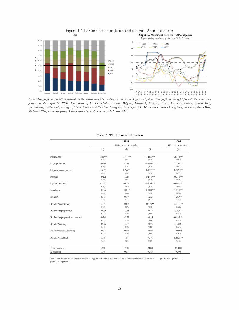
in the East Asian economies for a long period of time. As shown in Figure 1 Panel A, at the height of the

growth spur of the East Asian countries, Japan was indeed one of their main trading partners, for instance

representing more than 20 percent of trading for South Korea.1 Also suggestive of the active role of Japan as

a growth pole, i.e. source country for growth, its output comovement with those of the Tigers had been

particularly high during most of the 1980s (Figure 1, Panel B). Many observers have in fact described how the

Tigers “learned-by-doing” from their commercial relation with Japan: trading of similar goods while at the same

time integrating into their process of production.

Is the Japan-East Asian Tigers experience an idiosyncratic episode or is a connection to a growth

pole key in systematically triggering positive spillovers that may lead to higher growth rates? A very large

literature has actively discussed the role of trade in fostering economic development. For instance, Frankel

and Romer (1999) showed with data for 1985 that differences in the value of bilateral trade across countries

1 The simple average of bilateral trade of Indonesia, Thailand, Korea, Malaysia, Philippines, Taiwan, Singapore and Hong Kong was 21.1% in 1990.

3

were positively correlated with the levels of GDP per capita. Irwin and Tervio (2002) confirm those results

when including zero-trade data for a sample covering the period between 1913 and 1990. While those authors

have included a geographically-related instrument for trade, some papers later on derived a more proper

specification of the gravity equation as they put in evidence an important set of omitted variables, namely the

different institutional arrangements across countries. Taking into account these differences in institutions

across countries in the gravity equation lead to the lack of statistical significance of the coefficient of trade on

growth, as in for instance Acemoglu et al. (2001) and Rodrik et al. (2004). However the debate has not settled

with these papers, a number of papers keep pondering on the question of whether trade causes growth. For

example, Alcalá and Ciccione (2002) examined variables in PPP terms, rather than in nominal terms, and

while still using a gravity equation for trade and institutions, they found positive effects of these two variables

on productivity. Dollar and Kraay (2002) argues that both trade and institutions are important in the very

long run, but there is relatively larger role for trade over shorter horizons. Brückner and Lederman (2012)

provide evidence that trade causes growth for Sub-Saharan countries using a different set of instruments

(volume of rainfall). Noguer and Siscart (2005) argue that geographical controls must enter in the trade-

growth equation to avoid estimation biases, and re-estimate the fundamental equation with a greater number

of countries. They find that international trade does indeed promote growth.

The way in which trade effectively induces growth however remains largely under-tested in the

literature, particularly in a global context. Perhaps the mixed evidence with respect to the trade-growth nexus

is a reflection of the different nature of the trade relation across countries. International trade can be

beneficial for a country's economic development to the extent that it translates into greater factor

accumulation or productivity increases, especially those associated with technology diffusion and knowledge

spillovers. A direct mechanism of spillovers from one country to another is export demand, the simple

absorption of exports from given country fosters the expansion of its exporting industries. Another direct

mechanism of spillovers is through the technology embodied in the goods (both in physical and human

capital) that are exchanged between countries. Nevertheless, the indirect channels can impact economies in a

more significant way to the extent that it disseminates knowledge. Through the trade channel, imports may

4

contain intermediate goods and technologies unavailable to the recipient country. The greater the quantity of

these imports, the greater will potentially be the spillovers from trade. Exporters might also receive feedback

from importing nations (Blundell, Griffith and Reenen, 1995). Through FDI flows, technologies and

knowledge more broadly can be diffused from foreign parents to subsidiaries (directly or indirectly through

intermediate inputs), which may in turn spill to other firms in the host country through labor turnover for

instance (Aizenman and Sushko, 2011). Lastly, labor mobility, not only migration but also short-term business

travel, can promote knowledge spillovers by facilitating the diffusion of tacit technological knowledge (Oettl

and Agrawal, 2008).

Hence, in light of these spillover channels, the hypothesis of this paper is that some forms of trade

relations are more beneficial to long-term growth than others. In other words, this paper analyzes the nature

of trade relations and its effects on economic development. In particular, we focus on the industry

composition underlying the goods traded ("the industry channel"), the process of production of these goods,

and the type of products traded. To study the "industry channel", we focus on the degree of intra-industry

trade (IIT) between countries--various papers highlight that IIT is a good proxy for technological diffusion

and knowledge spillovers (Helpman and Krugman, 1989; Bernstein and Nadiri, 1988; Melitz, 2003; Bitzer and

Geishecker, 2005; and Badinger and Egger, 2010). Actually, the reallocation of firms towards more intra-

industry contributes to an increase in aggregate industry productivity. Another important aspect of the

industry channel explored here is the upstreamness embedded in goods traded from different industries as a

proxy for a country’s position in global production chains as for example in Antrás et al. (2012). UNCTAD’s

2011 World Investment Report emphasizes that in addition to being an important driver of trade flows

around the world, global value chains bring not only direct benefits (employment generation, direct local

value added, and export generation), but most importantly, indirect ones. They can act as catalysts for not

only technology and knowledge enhancement but also capacity-building and economic development more

widely, thus leading to virtuous cycles. Insertion into global value chains can thus affect the extent to which

trade fosters economic growth.

5

On the process of production channel, local producers can learn a great deal from the international

trade integration. Global buyers can induce how to improve production processes, attain consistency and

high quality, and increase the speed of the reaction to shocks (Keesing and lall, 1992; Piore and Ruiz Durán,

1998; Schmidtz and Knorringa, 2000). Hausmann et al. (2007) and Helpman (2008) argue that economies

grow when their firms or industries move into higher-value-added products through a process of discovering

new economic activities in which they can profitably engage. We examine whether some processes of

production are more prone to positive spillover effects than others--e.g. those relying on skilled labor versus

those relying on unskilled labor.

However, Hausmann et al. (2007) and Helpman (2008) defend that the technology, capital,

institutions, and skills needed to make these upgraded products are more easily adapted in some industries

than in others. Which brings to our last channel, the type of products traded. These authors, along with many

others, have argued that commodity production for instance is inherently associated with fewer positive

“spillover” effects to the extent that it creates less potential than other industries for developing linkages or

upgrading to more differentiated, higher-quality, higher-value products. Consistently, greater tech‐content of

imports has been associated with positive effects on economic development (Grossman and Helpman, 1991;

Eaton and Kortum, 2002; Rivera‐Batiz and Romer, 1991). In this paper, we analyze whether the type of

products traded plays any role in the way trade can lead to economic growth.

In the context where the composition of industries, the processes of production, and the types of

goods traded play an important role in the extent to which trade fosters economic growth, we also explore

whether different trading partners affect the trade-growth nexus. In fact, the successful experience of the

connection between the East Asian Tigers and Japan gives rise to an interesting hypothesis: whether trade

relations between a country and its main trading partner has similar effects to that of a country and a “world

growth pole.” The term “growth pole” should be understood in this text as a country (and its industries) that

is able to foster growth in other periphery countries through trade - rich linkages, multipliers, and spillover

effects are the key elements according to Adams-Kane and Lim (2011). Arora and Vamvakidis (2004) shows

in a panel estimation that trading partners’ growth and relative income level have a strong effect on domestic

6

growth. We look for refining this result by showing that “world growth pole” has a particular effect on

growth than any main trade partner.

Our findings highlight that the nature of trade plays a key role in explaining the trade-growth nexus,

thus going one step further than the traditional estimates of trade and growth. We provide some evidence

that the industries involved in bilateral trade relations have a substantial impact on growth. The more a

country exchange goods in the same industry with his commercial partners, the greater the impact on income

levels. This effect is further enhanced when such a relation takes place between the country and a world

growth pole. In addition, we also find that countries that export goods with a greater upstreamness potential

typically have greater income levels. Once more, this effect particularly important for the goods traded

between a country and world growth pole. Not only the industry channel, but also the process of production,

though not the types of goods per se, matter for overall economic development. Our findings suggest that

exports of goods that use skilled labor (hence, are intensive in human-capital) in their production process are

the prone to lead to positive growth spillovers than goods using unskilled labor. Moreover, there is strong

evidence that the effects of the nature of trade on income works mostly through total factor productivity

(TFP) rather than through the accumulation of physical or human capital. Lastly, we

The rest of the paper is organized as follows. Section 2 explains the methodology followed while

Section 3 describes the data used. Section 4 discusses the results. Finally, Section 5 concludes and draws some

policy implications.

2. Methodology

To analyze the effects of the nature of trade on growth, we consider an extended version of the specification

of Frankel and Romer (1999) by incorporating new developments in the literature. In particular, given our

focus on the effects of trade on growth, we add as a control variable the different institutional arrangements

across countries. We also take into account the size of the country by controlling for the size of the working

population and a country's area. Equation 1 shows the estimated equation:

7

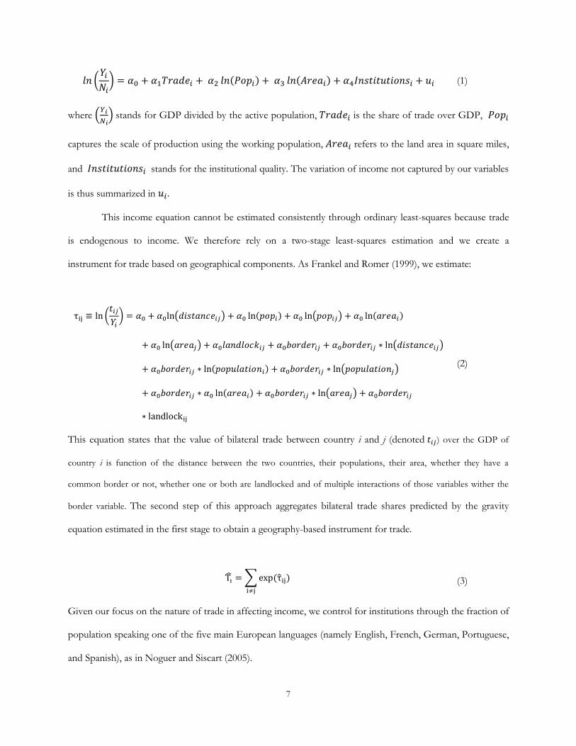
( ) ( ) ( ) (1)

where (

) stands for GDP divided by the active population, is the share of trade over GDP,

captures the scale of production using the working population, refers to the land area in square miles,

and stands for the institutional quality. The variation of income not captured by our variables

is thus summarized in .

This income equation cannot be estimated consistently through ordinary least-squares because trade

is endogenous to income. We therefore rely on a two-stage least-squares estimation and we create a

instrument for trade based on geographical components. As Frankel and Romer (1999), we estimate:

(

) ( ) ( ) ( ) ( )

( ) ( )

( ) ( )

( ) ( )

(2)

This equation states that the value of bilateral trade between country i and j (denoted ) over the GDP of

country i is function of the distance between the two countries, their populations, their area, whether they have a

common border or not, whether one or both are landlocked and of multiple interactions of those variables wither the

border variable. The second step of this approach aggregates bilateral trade shares predicted by the gravity

equation estimated in the first stage to obtain a geography-based instrument for trade.

∑ (

) (3)

Given our focus on the nature of trade in affecting income, we control for institutions through the fraction of

population speaking one of the five main European languages (namely English, French, German, Portuguese,

and Spanish), as in Noguer and Siscart (2005).

8

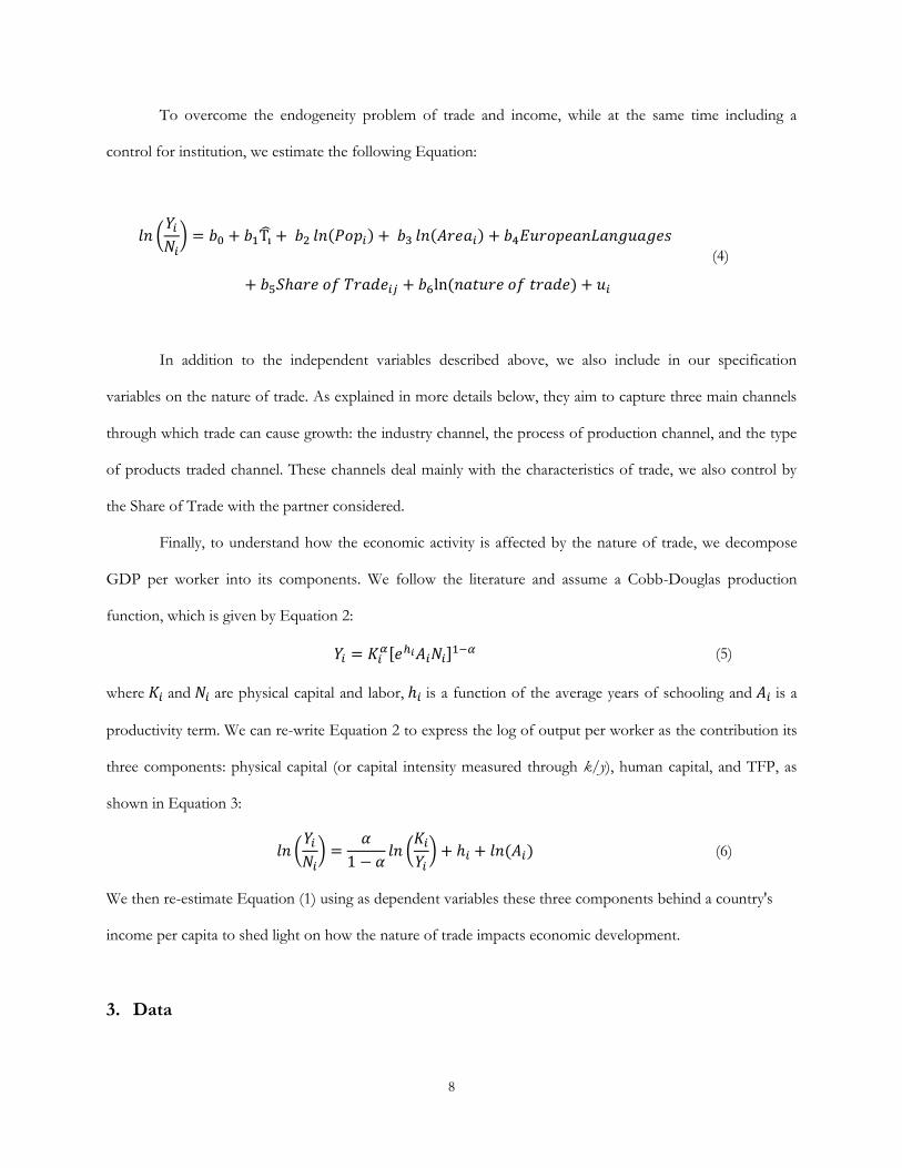
To overcome the endogeneity problem of trade and income, while at the same time including a

control for institution, we estimate the following Equation:

( ) ( ) ( )

( )

(4)

In addition to the independent variables described above, we also include in our specification

variables on the nature of trade. As explained in more details below, they aim to capture three main channels

through which trade can cause growth: the industry channel, the process of production channel, and the type

of products traded channel. These channels deal mainly with the characteristics of trade, we also control by

the Share of Trade with the partner considered.

Finally, to understand how the economic activity is affected by the nature of trade, we decompose

GDP per worker into its components. We follow the literature and assume a Cobb-Douglas production

function, which is given by Equation 2:

[ ]

(5)

where and are physical capital and labor, is a function of the average years of schooling and is a

productivity term. We can re-write Equation 2 to express the log of output per worker as the contribution its

three components: physical capital (or capital intensity measured through k/y), human capital, and TFP, as

shown in Equation 3:

( )

(

) ( ) (6)

We then re-estimate Equation (1) using as dependent variables these three components behind a country's

income per capita to shed light on how the nature of trade impacts economic development.

3. Data

9

One of the major novelties of our gravity model is the use data from 2000 to 2007, whereas most of the

literature has focused on past data, mostly from the 1980s and in few instances from the 1990s. To measure

the openness at country level, we use bilateral trade at the aggregate level for each country-pair from the

International Monetary Fund’s Direction of trade Statistics. Following Irwin and Terviö (2002), we added

zero-trade values between the two countries in each country-pair that did not report trade statistics. Indeed,

no trade between two countries is an important piece of information to understand the factors behind

countries choice of their commercial partners. Our results however are robust to the exclusion of these zero-

trade observations.

From the Penn World Tables, Mark 7.0, we obtain data on GDP in US$ and workforce.2 Country’s

area is taken from the World Development Indicators and is measured as the surface area in thousand square

miles. From Rose (2004), we obtained data on distance, landlocked countries, and common borders, variables

that we assumed constant and unchanged since 1999 for our sample of the 2000s.3 Our main proxy for

institutional quality is constructed using indicators from Kaufmann, Kraay, and Zoido-Lobatón (1999). As in

Alcalá and Ciccione (2004), we averaged the three indicators closer to the government anti-diversion policy

(GADP) index used by Hall and Jones (1999): government effectiveness, rule of law, and graft.

To construct detailed indicators of how countries trade, we used trade statistics disaggregated at

industry level from the World International Trade Statistics (WITS) of the United Nations. An important

aspect of our work resides in examining whether trading with a world growth pole is quantitatively similar to

trading with any other country (captured by countries' main trading partner). To this aim, we separate our

industry-level indicators in “overall”, that is, it captures a characteristic of trading relations between a country

and all its trading partners, and “with partner” which alternatively captures the nature of trading relations

between a country and its most important (in terms of volume of trade) world growth pole.

2 Workforce is obtained by dividing PPP GDP per capita by PPP GDP per worker and multiplying the result by population. 3 The variable capturing landlocked countries takes the value of 0, 1, or 2 for each country-pair.

10

To calculate the intra-industry trade index, we used data classified according to the SITC Rev.1 at the

2-digit level. The details of the basic index are given in Grubel and Lloyd (1975). 4 We simply adapted it to the

bilateral trade data. An index value of 0 represents a pure inter-industry trade, whereas an index value of 1

indicates a pure intra-industry trade.

Another important variable to understand the importance of the industry structure in a country's

welfare is the distance from final use of their exports, or what we have been referring to the upstreamness

potential embedded in a country's exports. Such upstreamness measure is a proxy for a country’s position in

global production chains as for example argued in Antrás et al. (2012). We used data disaggregated the 3-digit

level from SITC Rev. 3. The index takes values that range from 1 (final use output such as car and footwear)

to 4.65 (processing of raw materials, petrochemical).

We also study the influence of the process of production on growth. We used the classification of

Hinloopen and Van Marrewijk (2008) on factor intensity to determine which products are human-capital

intensive (as cutlery and watches). The data is extracted from SITC Rev. 3 at the 3-digit level.

Finally, we also examine whether the types of products traded have an influence on the overall level

of economic development. To deal with the notion of exports of commodities, we used the classification of

Lall (2000) that we adapted to SITC Rev. 1 data at the 3-digit level. Our classification considers 45 industries

as commodity-industries. With respect to the high-technology product as for instance aircraft or antibiotics,

the classification is taken from Eurostat for SITC Rev. 3 at 3-digit level.

In addition to exploring whether the nature of international trade can have an effect on economic

development, we examine whether trading with a world growth pole plays a particularly important role. Few

countries can be considered as world growth poles. We follow Adams-Kane and Lim (2011) in this regard.

The relevant growth poles over “the broad course of the history” have been the United States, China, and

4 We used the IIT index adjusted by trade imbalances. For a country j,

∑( ) ∑| |

∑( ) |∑ ∑ |, with i the industry at level 2-digit,

the exports of country j of product i to its trade partners and the imports of country j of product i from its trade partners.

11

Western Europe5. This choice is supported by the fact that over our period of study (2000-2007), those

countries represented 48% of the world GDP and 36.8% of total bilateral exchanges.

Lastly, the methodology implemented to decompose the level of income per capita, and thus total

factor productivity (TFP), follows Easterly and Levine (2001), Daude and Fernández-Arias (2010), and Daude

(2011), while considering some methodological insights from Hall and Jones (1999) and Klenow and

Rodríguez-Clare (1997). Equation 3 displays the functional form used to decompose GDP per capita into its

three components. First, we assume that the production function parameter is the same across countries,

and equal to 0.3. Second, the capital series are constructed using the Penn World Tables 7.0. In particular,

following Easterly and Levine (2001), we use the perpetual inventory method to construct the capital stock.

That is, we use:

( )

(4)

where is the stock of capital in period t for a country i,

is investment in period t for a country i, and is

the depreciation rate, assumed to be 0.07 for all countries. From Equation 4, and assuming steady state

conditions, the initial capital to GDP ratio is computed as: 6

(5)

where is the average investment-output ratio for the first ten years of the sample for country i and g is the

weighted average between world growth (weight of 0.75) of 4.23% and the average growth of the country

(weight of 0.25) for the first ten years of the sample.7 Then, to obtain the initial capital stock we multiply

Equation 5 by the average output of the first three years of the sample.

And lastly, for human capital, we follow Daude and Fernández-Arias (2010) coupled with the

standard approach of Hall and Jones (1999). We construct the human capital index h as a function of the

average years of schooling given by:

5 We proxy Western Europe by Germany, France, and United Kingdom. 6 We are assuming that the initial capital-to-GDP ratio is the steady state one. Daude and Fernández-Arias (2010) present some robustness checks showing that from 1970s onwards TFP measures are not very sensitive to initial conditions and assumptions. 7 For all the countries in our sample, we use 1970 as the starting point in order to avoid differences coming from the sample size.

12

( ( )) (6)

where the function ( ) is such that ( ) and ( ) is the Mincerian return on education. We

approximate this function with a piece-wise linear function. Based on Psacharopoulos (1994), we assume the

following rates of return for all the countries: 13.4 per cent for the first four years of schooling, 10.1 per cent

for the next four years, and 6.8 percent for education beyond the eight year. For each country in our sample,

we use the Barro-Lee (2010) data on the average years of schooling for the population older than 15 years.

Finally, following Mankiw, Romer, and Weil(1992) and Alcalá and Ciccione (2004), we dropped

countries for which the ratio of thousands of barrels of oil produced per day to GDP exceeded 200,000 in

1985. Consistent with the criteria in Alcalá and Ciccione (2004), the major oil producers in our sample are

Angola, Gabon, Congo, Iraq, Oman, Kuwait, Qatar, Saudi Arabia, and the United Arab Emirates.

4. Main Results

4.1 The basic empirical model

As described in Section 2, we adopt an instrumental variable approach to deal with the endogeneity of trade

and income. First, we construct a geography-based instrument for trade. We construct this instrument

estimating the gravity model described in equation 2 and regress the bilateral degree of openness (captured by

exports plus imports) on variables such as distance, population, and area.

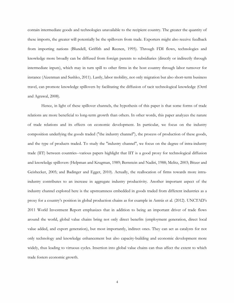
Table 1 reports estimates of the first stage equation. While consistent with the findings in the

literature, we find evidence suggesting significant changes on the relationship of openness with geographical

variables in recent years. For comparison purposes we report in the first column the results from Frankel and

Romer (1999), while the second column shows the results of Noguer and Siscart (2005), both from 1985 and

without zero-trade data included. To show the consistency of our results with those found in the existing

literature, we report in the third column our own estimation of equation 2. Our estimates show similar

patterns to those in columns (1) and (2).8 We construct an instrument for trade in the 2000s by estimating

equation 2 for every year in our sample. The fourth column shows our estimation for 2005 as an example,

8 The differences in the results are due to an increase number of observations for 1985 made possible with the actualization of the Penn World Tables, Mark 7.0.

13

though the estimations are qualitatively similar for the other years in our sample. The more recent period

study and the inclusion of zero-trade data as in Irwin and Terviö (2002) modify slightly the results respect to

1985.9 Column (4) presents our bilateral equation for 200510. The effects are generally higher than in the

benchmark results. Distance seems to play a stronger negative role in 2005 than in 1985, in line with the

results of Brun, Carrère, Guillaumont and de Melo (2005). Population of the trading partner plays greater role

when zero-trade values are included.

[Insert table 1]

From the bilateral equation, we retrieve fitted values for bilateral trade, aggregated at the country

level, to obtain a geographic-based instrument for trade, as shown in equation 3. We then estimate the second

stage of the 2SLS approach by estimating a between effects panel regression over the entire sample period.

4.2 The Nature of Trade and Its Effects on Output

In this section, we provide evidence that not only the volume of trade is important, but also its nature. By

nature of trade, we refer to the industries involved in the exchange of goods (the "industry" channel), the

process of production of the traded goods (the "process of production" channel), and the types of products

traded (the "type of products" channel).

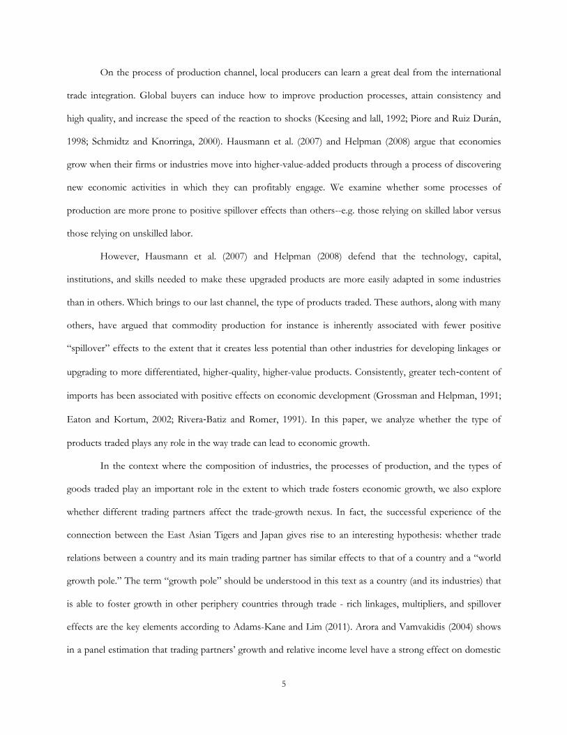
Table 2 gives the benchmark of our work, showing the regression of equation 4 without any variables

on the nature of trade. Column (1) gives the results when the share of trade with the main partner is

integrated in the regression whereas column (2) integrates the share of trade with the main world growth. The

coefficient of trade is similar in both columns; an increase of one percentage point in trade openness would

lead to an increase of 3 percent of the GDP per capita for an average country. We introduce the log of

population and the log of area in our estimates as Irwin and Tervio (2002). The share of trade is the only

partner-specific variable of this regression. We note that the more important the main partner is over the total

9 Frankel and Romer (1999) dropped zero-trade data information. Irwin and Tervio (2002) show values of trade of zero are an important piece of information that should not be dropped from the regression estimations. We follow the authors and add to all the value of bilateral trade one dollar that is insignificant for the value when trade really and that permit us to introduce a very small value of trade that we could approximate to zero. 10 Our sample that extends from 2000 to 2007.

14

trade of a country, the worse it is for its GDP per capita. The diversity of trading partners seems to be

positively correlated to the growth of the outcome per capita. Nevertheless, when we consider the share of

trade with the main world growth pole, diversity is not statistically significant. This result suggests that

diversifying the partners is positive whereas in the case of the partner is a world growth pole. Finally, the

institution control is strongly significant in each regression.

[Insert table 2]

To examine the "industry channel", we focus on two indexes. First, we analyze the degree of intra-

industry trade between countries. Second, we evaluate the upstreamness embedded in goods traded from

different industries as a proxy for a country’s position in global production chains.

Table 3 presents the results for the IIT index. Results in table 3 are extensions of the benchmark

model presented in column 1 of Table 2. We add the IIT index for country against all its partners (called “IIT

– Overall”). The index evaluates at which level a country exports and imports in the same industry: an index

value of 0 represents a pure inter-industry trade, while an index value of 1 indicates a pure intra-industry

trade. The index is calculated with a disaggregation of the data at 2-digit level that permits a consistent

definition of the IIT in order to interpret the index as a way of learning for a country. For instance, coffee, tea

and cocoa are considered in the same industry. The first column of table 3 shows a strong coefficient highly

significant on the GDP per capita. A marginal increase of the overall IIT, i.e. a global movement to more

intra-industry for a country, contributes to an average increase of 3.1 percent of the GDP per capita. The

effect is well-known in the literature.

One of the goals of this paper is to demonstrate that a privileged relation with a world growth pole is

central. In order to stand out the influence of the Pole, we take as benchmark the relation of the country with

its main commercial partner, defined very simply as the partner country with which the imports and exports

are the most important. The IIT index is then recalculated between the country and its main partner. This

index is called “IIT – with partner” and the results are reported in Column (2). The magnitude of the effect

on the GDP per capita is similar as the IIT overall. Interestingly, the third column shows that when both IIT

15

overall and IIT with the main partner are regressed simultaneously, only the coefficient associated to the later

is statistically significant. This is a first step to understand the importance of the IIT in a bilateral relation.

The results from the second panel of results titled “World Growth Pole” are presented in columns

(4) to (6) and change only the bilateral variable to the world growth pole from main commercial partner. We

define the world growth pole of each country by the maximum bilateral trade between the country and one of

the three following poles: the USA, China or Western Europe. Annex 1 shows for each country, the main

partner and the main world growth pole considered for 200511. There are some countries for which the two

partners are the same. For instance, Mexico’s main partner and main world growth pole are the United States

of America. But this is not always the case. For example, the main partner of Afghanistan is Pakistan which is

not as a world growth pole. As a consequence, the United States of America is the main world growth pole

for Afghanistan. Column (4) is similar to Column (1) respect to the IIT index overall, as only the variable

Share of Trade differs between both regressions. The fifth column presents the results of the estimates of the

coefficient of IIT with the partner, which is in this case the main growth pole. The coefficient associated is

very high and imply that a marginal increase of the intra-industry trade with the pole would raise in average

the GDP per capita of 3.8 percent. This result is statistically significant at one percent. Finally, Column (6)

shows the interaction of the IIT overall and of the IIT with the main world growth pole. Only the coefficient

of IIT associated with the main world growth pole is statistically significant and not IIT Overall.

We find evidence that having a high coefficient of IIT with a partner (being the Main Partner or the

Growth Pole) is always better for growth than having a high intra-industry trade in overall (which is in turn

better than not having intra-industry trade with anybody!). Nevertheless, an interesting fact is that the effect

of IIT with the world growth pole is higher than the effect of IIT with the main partner, suggesting that

trading in the same industry as a pole is more prone to generate output than any other trade relation. Column

(5) shows a coefficient of IIT with pole much stronger than the IIT with main partner (Column 2). A

marginal increase of the IIT with the pole contributes to an average increase nearly 30 percent superior than a

marginal increase of the IIT with the main partner. Column (6) induces that the IIT with the Pole is more

11 The selection of the main partner and of the main world growth pole has been realized for each year of the panel

16

important than the overall, and in a magnitude superior to Column (3). This result can be interpreted as a

higher efficiency of the main world growth pole to transmit technology, process of production, and more

generally knowledge to a specific industry of a country. By importing and exporting products of the same

industry, countries learn from the most efficient firms in the firm (that are without doubts located in the

USA, China and Western Europe).

[Insert table 3]

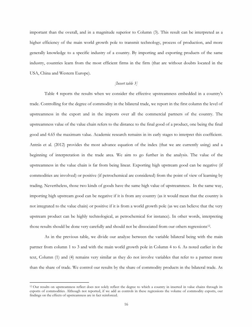
Table 4 reports the results when we consider the effective upstreamness embedded in a country's

trade. Controlling for the degree of commodity in the bilateral trade, we report in the first column the level of

upstreamness in the export and in the imports over all the commercial partners of the country. The

upstreamness value of the value chain refers to the distance to the final good of a product, one being the final

good and 4.65 the maximum value. Academic research remains in its early stages to interpret this coefficient.

Antrás et al. (2012) provides the most advance equation of the index (that we are currently using) and a

beginning of interpretation in the trade area. We aim to go further in the analysis. The value of the

upstreamness in the value chain is far from being linear. Exporting high upstream good can be negative (if

commodities are involved) or positive (if petrochemical are considered) from the point of view of learning by

trading. Nevertheless, those two kinds of goods have the same high value of upstreamness. In the same way,

importing high upstream good can be negative if it is from any country (as it would mean that the country is

not integrated to the value chain) or positive if it is from a world growth pole (as we can believe that the very

upstream product can be highly technological, as petrochemical for instance). In other words, interpreting

those results should be done very carefully and should not be dissociated from our others regressions12.

As in the previous table, we divide our analyze between the variable bilateral being with the main

partner from column 1 to 3 and with the main world growth pole in Column 4 to 6. As noted earlier in the

text, Column (1) and (4) remains very similar as they do not involve variables that refer to a partner more

than the share of trade. We control our results by the share of commodity products in the bilateral trade. As

12 Our results on upstreamness reflect does not solely reflect the degree to which a country in inserted in value chains through its exports of commodities. Although not reported, if we add as controls in these regressions the volume of commodity exports, our findings on the effects of upstreamness are in fact reinforced.

17

we analyze later, none of the coefficient associated is statistically significant, with the exception of the bilateral

value of trade of commodities with the main world growth pole. The upstreamness in the value chain of

exported products seems positive and weakly statistically significant whereas the upstreamness in the value

chain of imported products appears negative. Being at the top of the chain value in its products exported is

positive as it demonstrates a strong integration to the international production, always when it is not about

commodities. At the opposite, importing very high upstream products is probably negative if we consider all

the trade partners of the country13, as we can imagine that a high share of those products are commodities.

This result is in a sense confirmed in the second column. When we focus on a particular bilateral relationship

between the country and its main partner, the value of upstreamness in the exports as in the imports is not

anymore statistically significant. It is not in a special relationship that upstream products are not beneficial to

growth (after all, basic products will ever be needed to all productions), the problem appears when products

traded are always basics. Column (3) does not differ from the previous column: the overall index of

upstreamness mimics the first column but no variable associated with the main partner is statistically

significant.

At the contrary, the fifth column added an information respect to the value of upstreamness in the

exports. The index showing the relationship with the main world growth pole is statistically significant at one

percent. A marginal increase in this index would lead to an increase of 2.8 percent of the country’s GDP. This

value is positive and statistically significant. We can interpret this effect by inferring that high upstream

products exported to a world growth pole could have the advantage of having the feedback of countries able

to bring growth. Indeed, those products respond to a demand and carry in themselves a value added of being

required in an international process of production. On the other hand, the upstreamness of the value chain in

the imports is not statistically significant. Column (6) includes all the variables. If the variable with the main

world growth pole are not anymore statistically significant, they remain with the right sign, and the overall

value are still statistically significant.

13 The coefficient associate with the upstreamness in the import is not significant in the first column, but it is in column (4). We choose to interpret the coefficient column 4 as they are closed.

18

To sum up, our estimations provide evidence that greater the upstreamness potential embedded in a

country's exports is positively and significantly associated with high income levels, thus suggesting the

positive spillover effects of being inserted into global value chains. Importantly, the effect on a bilateral basis

is significant only when the trading relation concerns the country and a world growth pole.14 The degree of

upstreamness in a country's import has no statistically significant effect on the level of income per capita

across countries. A probable explanation is that furnishing a world growth pole, the country will learn from

its clients and will ameliorate its production.

The second channel though which trade can have an effect on growth is through the process of

production. For instance, local producers can learn a great deal from the international trade integration.

Global buyers can induce how to improve production processes, attain consistency and high quality, and

increase the speed of the reaction to shocks. Hausmann et al. (2007) and Helpman (2008) argue that

economies grow when their firms or industries move into higher-value-added products through a process of

discovering new economic activities in which they can profitably engage. We examine whether some

processes of production are more prone to positive spillover effects than others--e.g. those relying on skilled

labor versus those relying on unskilled labor.

[Insert table 4]

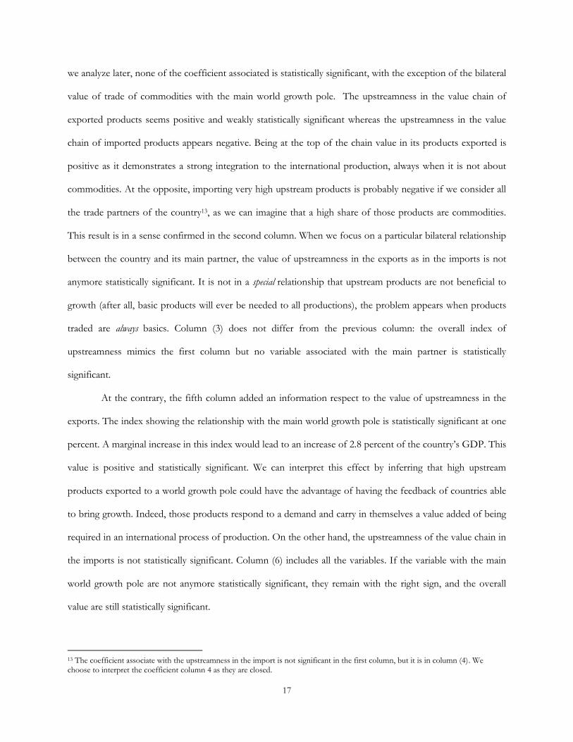
Table 5 shows that producing goods with a high intensity of human-capital factors is positively

associated with greater levels of income per capita. Column (1) as Column (4) show a similar regression where

more skilled-labor intensive goods are traded more the consequences are positive on the output per capita.

This result, even if it is smaller, remains true when the trade with only the main partner is analyzed (column

2). Nevertheless, when both products with high human-capital intensive product on the overall and with the

main partner are introduced, no variables are anymore statistically significant, as shown in Column (3).

The regressions involving main world growth pole give stronger and higher results. The coefficient

reported in the fifth column is 18 percent higher than the one reported in the second column: trading

products for which the process of production requires high-skill labor generates 18 percent more increase of

14 In Annex 2, we report the results of the decomposition of the upstreamness index in exports by fringes.

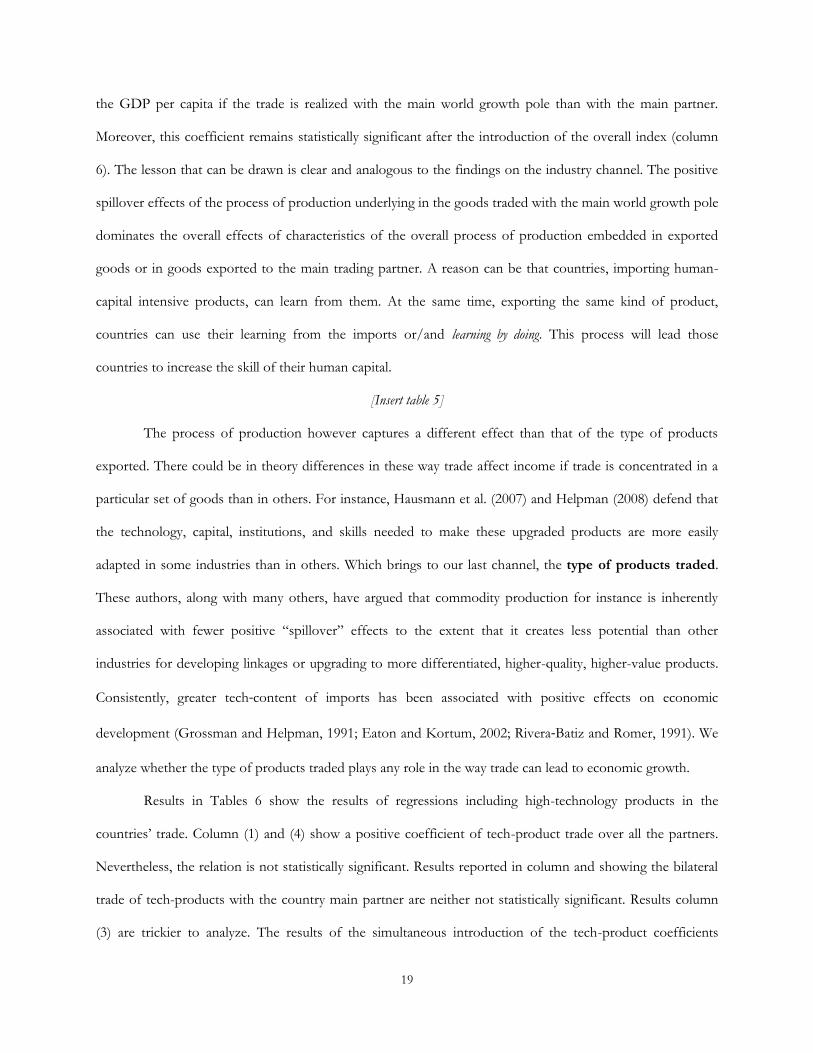
19

the GDP per capita if the trade is realized with the main world growth pole than with the main partner.

Moreover, this coefficient remains statistically significant after the introduction of the overall index (column

6). The lesson that can be drawn is clear and analogous to the findings on the industry channel. The positive

spillover effects of the process of production underlying in the goods traded with the main world growth pole

dominates the overall effects of characteristics of the overall process of production embedded in exported

goods or in goods exported to the main trading partner. A reason can be that countries, importing human-

capital intensive products, can learn from them. At the same time, exporting the same kind of product,

countries can use their learning from the imports or/and learning by doing. This process will lead those

countries to increase the skill of their human capital.

[Insert table 5]

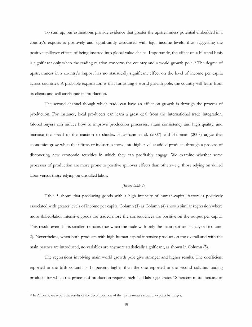
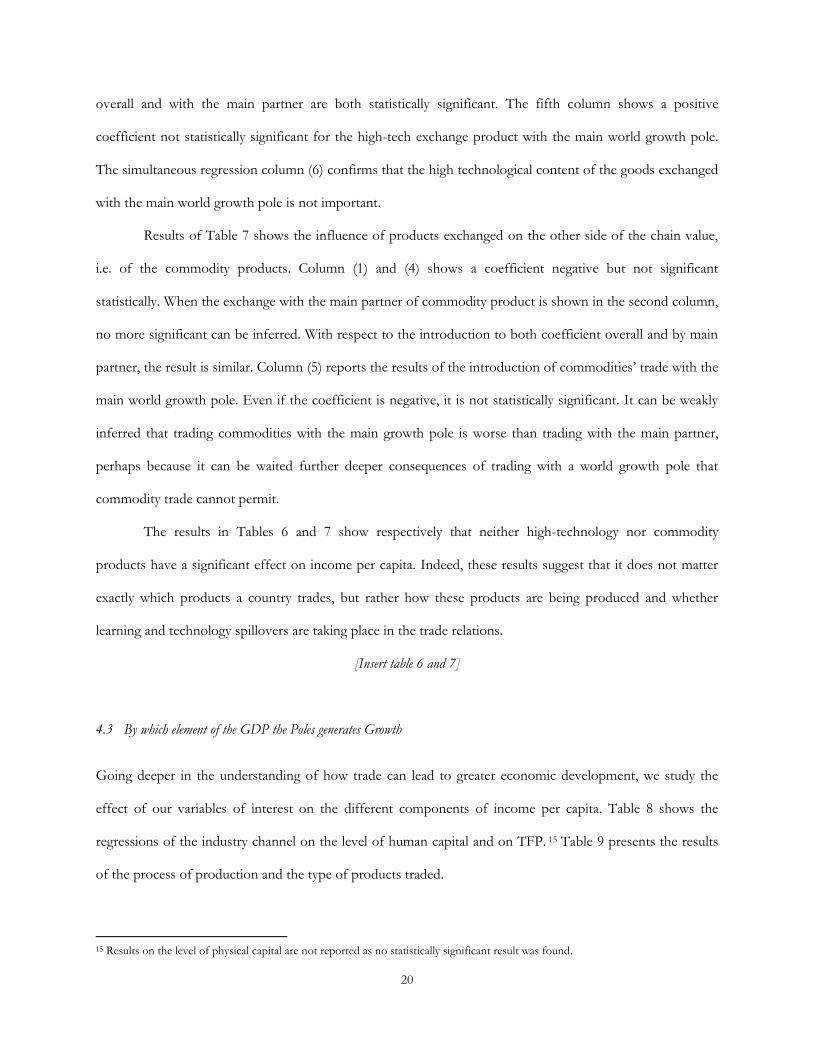
The process of production however captures a different effect than that of the type of products

exported. There could be in theory differences in these way trade affect income if trade is concentrated in a

particular set of goods than in others. For instance, Hausmann et al. (2007) and Helpman (2008) defend that

the technology, capital, institutions, and skills needed to make these upgraded products are more easily

adapted in some industries than in others. Which brings to our last channel, the type of products traded.

These authors, along with many others, have argued that commodity production for instance is inherently

associated with fewer positive “spillover” effects to the extent that it creates less potential than other

industries for developing linkages or upgrading to more differentiated, higher-quality, higher-value products.

Consistently, greater tech‐content of imports has been associated with positive effects on economic

development (Grossman and Helpman, 1991; Eaton and Kortum, 2002; Rivera‐Batiz and Romer, 1991). We

analyze whether the type of products traded plays any role in the way trade can lead to economic growth.

Results in Tables 6 show the results of regressions including high-technology products in the

countries’ trade. Column (1) and (4) show a positive coefficient of tech-product trade over all the partners.

Nevertheless, the relation is not statistically significant. Results reported in column and showing the bilateral

trade of tech-products with the country main partner are neither not statistically significant. Results column

(3) are trickier to analyze. The results of the simultaneous introduction of the tech-product coefficients

20

overall and with the main partner are both statistically significant. The fifth column shows a positive

coefficient not statistically significant for the high-tech exchange product with the main world growth pole.

The simultaneous regression column (6) confirms that the high technological content of the goods exchanged

with the main world growth pole is not important.

Results of Table 7 shows the influence of products exchanged on the other side of the chain value,

i.e. of the commodity products. Column (1) and (4) shows a coefficient negative but not significant

statistically. When the exchange with the main partner of commodity product is shown in the second column,

no more significant can be inferred. With respect to the introduction to both coefficient overall and by main

partner, the result is similar. Column (5) reports the results of the introduction of commodities’ trade with the

main world growth pole. Even if the coefficient is negative, it is not statistically significant. It can be weakly

inferred that trading commodities with the main growth pole is worse than trading with the main partner,

perhaps because it can be waited further deeper consequences of trading with a world growth pole that

commodity trade cannot permit.

The results in Tables 6 and 7 show respectively that neither high-technology nor commodity

products have a significant effect on income per capita. Indeed, these results suggest that it does not matter

exactly which products a country trades, but rather how these products are being produced and whether

learning and technology spillovers are taking place in the trade relations.

[Insert table 6 and 7]

4.3 By which element of the GDP the Poles generates Growth

Going deeper in the understanding of how trade can lead to greater economic development, we study the

effect of our variables of interest on the different components of income per capita. Table 8 shows the

regressions of the industry channel on the level of human capital and on TFP. 15 Table 9 presents the results

of the process of production and the type of products traded.

15 Results on the level of physical capital are not reported as no statistically significant result was found.

21

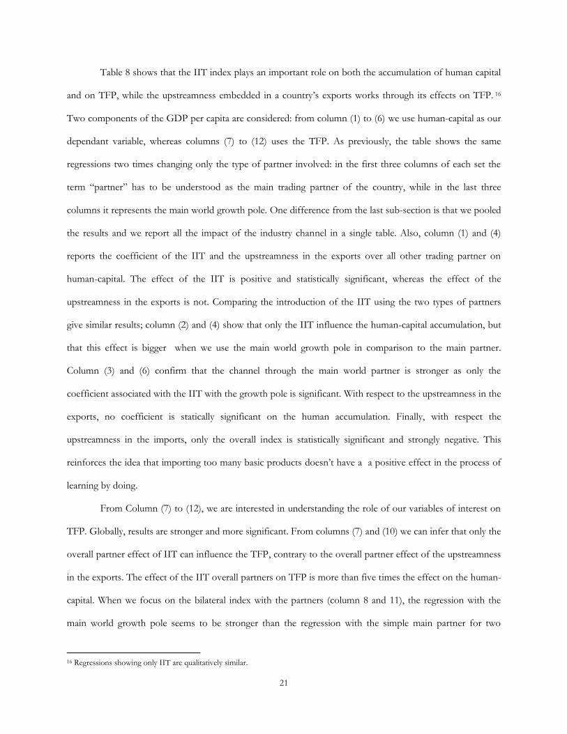
Table 8 shows that the IIT index plays an important role on both the accumulation of human capital

and on TFP, while the upstreamness embedded in a country’s exports works through its effects on TFP. 16

Two components of the GDP per capita are considered: from column (1) to (6) we use human-capital as our

dependant variable, whereas columns (7) to (12) uses the TFP. As previously, the table shows the same

regressions two times changing only the type of partner involved: in the first three columns of each set the

term “partner” has to be understood as the main trading partner of the country, while in the last three

columns it represents the main world growth pole. One difference from the last sub-section is that we pooled

the results and we report all the impact of the industry channel in a single table. Also, column (1) and (4)

reports the coefficient of the IIT and the upstreamness in the exports over all other trading partner on

human-capital. The effect of the IIT is positive and statistically significant, whereas the effect of the

upstreamness in the exports is not. Comparing the introduction of the IIT using the two types of partners

give similar results; column (2) and (4) show that only the IIT influence the human-capital accumulation, but

that this effect is bigger when we use the main world growth pole in comparison to the main partner.

Column (3) and (6) confirm that the channel through the main world partner is stronger as only the

coefficient associated with the IIT with the growth pole is significant. With respect to the upstreamness in the

exports, no coefficient is statically significant on the human accumulation. Finally, with respect the

upstreamness in the imports, only the overall index is statistically significant and strongly negative. This

reinforces the idea that importing too many basic products doesn’t have a a positive effect in the process of

learning by doing.

From Column (7) to (12), we are interested in understanding the role of our variables of interest on

TFP. Globally, results are stronger and more significant. From columns (7) and (10) we can infer that only the

overall partner effect of IIT can influence the TFP, contrary to the overall partner effect of the upstreamness

in the exports. The effect of the IIT overall partners on TFP is more than five times the effect on the human-

capital. When we focus on the bilateral index with the partners (column 8 and 11), the regression with the

main world growth pole seems to be stronger than the regression with the simple main partner for two

16 Regressions showing only IIT are qualitatively similar.

22

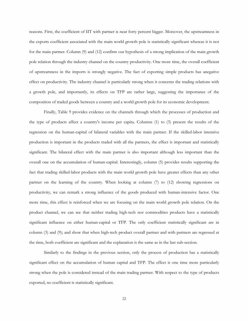
reasons. First, the coefficient of IIT with partner is near forty percent bigger. Moreover, the upstreamness in

the exports coefficient associated with the main world growth pole is statistically significant whereas it is not

for the main partner. Column (9) and (12) confirm our hypothesis of a strong implication of the main growth

pole relation through the industry channel on the country productivity. One more time, the overall coefficient

of upstreamness in the imports is strongly negative. The fact of exporting simple products has anegative

effect on productivity. The industry channel is particularly strong when it concerns the trading relations with

a growth pole, and importantly, its effects on TFP are rather large, suggesting the importance of the

composition of traded goods between a country and a world growth pole for its economic development.

Finally, Table 9 provides evidence on the channels through which the processes of production and

the type of products affect a country's income per capita. Columns (1) to (3) present the results of the

regression on the human-capital of bilateral variables with the main partner. If the skilled-labor intensive

production is important in the products traded with all the partners, the effect is important and statistically

significant. The bilateral effect with the main partner is also important although less important than the

overall one on the accumulation of human-capital. Interestingly, column (5) provides results supporting the

fact that trading skilled-labor products with the main world growth pole have greater effects than any other

partner on the learning of the country. When looking at column (7) to (12) showing regressions on

productivity, we can remark a strong influence of the goods produced with human-intensive factor. One

more time, this effect is reinforced when we are focusing on the main world growth pole relation. On the

product channel, we can see that neither trading high-tech nor commodities products have a statistically

significant influence on either human-capital or TFP. The only coefficient statistically significant are in

column (3) and (9); and show that when high-tech product overall partner and with partners are regressed at

the time, both coefficient are significant and the explanation is the same as in the last sub-section.

Similarly to the findings in the previous section, only the process of production has a statistically

significant effect on the accumulation of human capital and TFP. The effect is one time more particularly

strong when the pole is considered instead of the main trading partner. With respect to the type of products

exported, no coefficient is statistically significant.

23

[Insert table 9]

4.4 Differentiating World Growth Poles: Developed versus Emerging poles

As we mentioned in the introduction, the aim of the paper is to investigate whereas the Tiger’s growth is an

idiosyncratic episode or if a connection to a growth pole is key in systematically triggering positive spillovers

that may lead to higher growth rates. Up to this point, we analyzed the importance of trading with a world

growth pole in general, without distinguishing between the countries we considered. As explained in the data

section, we defined the world growth pole following Adams-Kane and Lim (2011). The relevant growth poles

over “the broad course of the history” have been the United States, Western Europe and China.

Nevertheless, the success story of the Tigers is perhaps not independent from the pole to which they have

been linked. Indeed, Japan was more developed that the East Asian countries. In this section, we decided to

test whether the level of development of the world growth pole influences the spillover of the trade’s nature

on growth. For this, we separated the world growth poles in two categories: the developed growth poles which

combine the United States and the Western Europe; and the emerging growth pole defined by China. Our

hypothesis resulting from the successful connection between Japan and the Tigers is that a developed pole is

more prone to help impulse a sustainable growth.

Table 10 provides evidence in favor of our hypothesis. The results are separated in two parts: after

the lines of controls, we categorize the bilateral indicators alternatively with developed countries and with

emerging countries. Overall the columns, we remark that the share of trade with developed countries tends to

be positive and sometimes statistically significant whereas the share of trade with emerging countries is

constantly negative although never significant. This is a first step to distinguish between the effect of trading

with USA and Western Europe or with China. The first column of Table 10 provides the results of the intra-

industry trade index with the two alternative partners considered. Only the coefficient associated with

developed countries is statistically significant. It is estimated that a marginal increase of the IIT index leads to

an increase of more than 3.3 percent in the GDP per capita. On the contrary, the index of IIT in relation with

emerging countries is not significant. Going further in our analysis, the column (2) provides results of the

24

other part of the industry channel. Controlling by the export of commodities, we remark that no variables of

upstreamness are statistically significant when we consider bilateral relation with a developed country.

However, the value of the coefficient of the upstreamness in the imports is statistically significant at 1 percent

when we consider the relation with an emerging country. This reinforces a hypothesis previously issued:

importing highly upstreamned products (i.e. the one at the top of the value chain) from an emerging country

is not positive for the growth of output per capita. In fact, we can imagine that coming from a developed

country, the very upstream product can be more beneficial as they can be petrochemical or so. Nevertheless,

coming from emerging market, those upstream products are without doubts much closer to commodities or

very primary products.

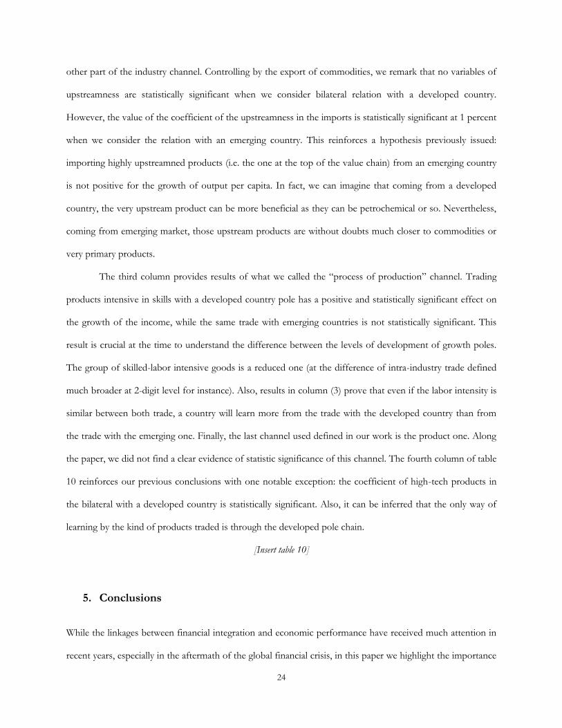
The third column provides results of what we called the “process of production” channel. Trading

products intensive in skills with a developed country pole has a positive and statistically significant effect on

the growth of the income, while the same trade with emerging countries is not statistically significant. This

result is crucial at the time to understand the difference between the levels of development of growth poles.

The group of skilled-labor intensive goods is a reduced one (at the difference of intra-industry trade defined

much broader at 2-digit level for instance). Also, results in column (3) prove that even if the labor intensity is

similar between both trade, a country will learn more from the trade with the developed country than from

the trade with the emerging one. Finally, the last channel used defined in our work is the product one. Along

the paper, we did not find a clear evidence of statistic significance of this channel. The fourth column of table

10 reinforces our previous conclusions with one notable exception: the coefficient of high-tech products in

the bilateral with a developed country is statistically significant. Also, it can be inferred that the only way of

learning by the kind of products traded is through the developed pole chain.

[Insert table 10]

5. Conclusions

While the linkages between financial integration and economic performance have received much attention in

recent years, especially in the aftermath of the global financial crisis, in this paper we highlight the importance

25

of trade in goods for growth. We provide robust evidence that trade significantly affects income, and that

some ways of trading are more beneficial than others. Using a two-stage least-square methodology, we

explored three main characteristics of trading relations and to what extent they explain how trade causes

growth: the industry (capturing the composition of exports and imports between countries), the process of

production (proxying for instance the intensity of skilled labor used in the production of traded goods), and

the types of products traded. These three characteristics are explored against three dimensions of trading

partners: the overall aggregate trade characteristics underlying a country’s trading relations with the rest of the

world, with its main trading partner, and with its main world growth pole partner. Overall, we find that the

nature of trading relations (products and partners) matter a great deal to whether (and thus how) trade causes

growth. In particular, trading with a world growth pole, particularly a developed country ones, leads to greater

growth spillovers than trading with any other commercial partner. This relation is reinforced when a country

and its main world growth pole trade similar products (i.e. in the same industry) and when they trade high-

skilled products. In addition, being part of value chains is also beneficial to growth, especially when a country

in on the supplier side through its exports with large upstream potential. Such an effect holds even if we

control for the share of commodity products being exported. In fact, no statistically significance was found in

trading any particular type of good per se, be it commodity or high-tech products, suggesting that it is not the

type of product traded that is important, but rather the process of production underlying traded goods.

Moreover, these results indicate that the process of learning is a key underlying channel through which trade

causes growth. For instance, trading goods within the same industry, being integrated into value chains, and

exchanging high-skilled goods have all been shown to significantly affect the trade-growth relation, and thus

pointing towards a more specific type of trading relations more prone to generate learning.

These findings have many policies implications. On the one hand, many developing countries are

relatively closed, in their early phases of integration into the global goods trade. For these countries, finding

the optimal conditions under which trade generates growth allows them to better design their policies and

shape incentives in a compatible manner to avoid much of the downsides associated with greater integration

into world markets. For instance, our paper has highlighted the importance of trading with a world growth

26

pole in generating output per capita growth. The intra-industry trade is also a process that enhances growth

spillovers. On the other hand, for countries already integrated into global markets, our results suggest that

policies should be focused more on production upgrades, in moving towards products with greater value

added to the extent that there is greater scope for learning from their partners, particularly form the world

growth poles. This seems particularly important for commodity exporters. Nonetheless, the results in this

paper suggest that trade can lead to a sustainable growth to the extent that it is associated with technology

transfer and learning across countries, independent of their stage of development.

References Acemoglu, D., Johnson, S. and J. Robinson, 2001. “The Colonial Origins of Comparative Development: An

Empirical Investigation,” American Economic Review Vol. 91(5), pp. 1369-1401. Adams-Kane, J. and J. J. Lim, 2011. “Growth Poles and Multipolarity” World Bank Policy Research Working

Paper No. 5712. Aizenman, J. and V. Sushko, 2011. “Capital flows: Catalyst or Hindrance to economic takeoffs?” NBER

Working Paper No. 17258. Alcalá, F. and A. Ciccone, 2004. “Trade and Productivity”, Quarterly Journal of Economics Vol. 119(2), pp. 612-

645. Antrás, P., Chor, D., Fally, T. and R. Hillberry 2012.“Measuring the Upstreamness of Production and Trade

Flows’,’ American Economic Review (forthcoming) Arora, V. and A. Vamvakidis 2004. “How much Do Trading Partners Matter for Economic Growth?”, IMF

Working Paper, WP/04/26. Badinger, H. and P. Egger, 2008. "Intra- and Inter-Industry Productivity Spillovers in OECD Manufacturing:

A Spatial Econometric Perspective," CESifo Working Paper Series 2181. Bitzer, J. and Geishecker, I., 2006. “What drives trade-related R&D spillovers? Decomposing knowledge-

diffusing trade flows”, Economics Letters, Elsevier, vol. 93(1), pages 52-57. Barro, R. and J.W. Lee, 2010. "A New Data Set of Educational Attainment in the World, 1950-2010", NBER

Working Paper No. 15902. Bernstein, J. I. and M. I. Nadiri, 1989. "Research and Development and Intra-industry Spillovers: An

Empirical Application of Dynamic Duality," Review of Economic Studies Vol. 56(2), pages 249-67. Bitzer, Jurgen and Geishecker, Ingo, 2006. "What drives trade-related R&D spillovers? Decomposing

knowledge-diffusing trade flows," Economics Letters Vol. 93(1), pages 52-57. Blundell, R. Griffith, R. and J. Van Reenen, 1995. "Dynamic Count Data Models of Technological

Innovation," Economic Journal Vol. 105(429), pages 333-44. Brückner, M. and D. Lederman,2012. “Trade Causes Growth in Sub-Saharan Africa”, World Bank Policy

Research Working Paper No. 6007. Brun, J.-F., Carrère, C., Guillaumont, P., and J. de Melo, 2005. “Has Distance Died? Evidence from a Panel

Gravity Model”, World Bank Economic Review Vol.19 (1), pp. 99-120. Daude, C. ,2011. “Growth and productivity in Latin America: What is Missing?” OECD Development

Centre, mimeo. Daude, C. and E. Fernández-Arias, 2010. “On the Role of Productivity and Factor Accumulation in

Economic Development in Latin America and the Caribbean”, IDB Working Paper series IDB-WB-155.

http://ideas.repec.org/s/tpr/qjecon.html

27

Dollar, D. and A. Kraay, 2002. “Institutions, Trade, and Growth”, World Bank Policy Research Working Paper No. 3004.

Easterly, W., and R. Levine, 2001. “What Have We Learned from a Decade of Empirical Research on Growth? It’s Not Factor Accumulation: Stylized Facts and Growth Models,” World Bank Economic Review 15(2), pages 177-219.

Eaton, J. and S. Kortum, 2002, “Technology, Geography, and Trade,” Econometrica, 70(5), pages 1741–1779. Frankel, J.A. and D. Romer, 1999. “Does Trade Cause Growth?” American Economic Review Vol. 89 (3), 1999),

pages. 379-399. Grossman, G. M. and E. Helpman, 1991. “Quality Ladders in the Theory of Growth”, Review of Economic

Studies Vol. 58 (1), pages 43-61. Keesing, D. and S. Lall, 1992. “Marketing Manufactured Exports From Developing Countries: Learning

Sequences and Public Support”, in G. Helleiner (ed.), Trade Policy, Industrialization and Development, Oxford: Oxford University Press, pages 176–93.

Klenow, P., and A. Rodríguez-Clare, 1997. “The Neoclassical Revival in Growth Economics: Has It Gone Too Far?” NBER Macroeconomics Annual 1997.

Hall, R. E. and Jones, C. I. “Why Do Some Countries Produce So Much More Output Per Worker Than Others?” Quarterly Journal of Economics Vol. 114(1), pages 83-116.

Helpman, E. and P. Krugman, 1987. Market Structure and Foreign Trade: Increasing Returns, Imperfect Competition, and the International Economy, MIT Press Books, The MIT Press.

Hinloopen, J., and C. van Marrewijk (2004), "Dynamics of Chinese Comparative Advantage," Tinbergen Institute Discussion Paper 04-034/2.

Irwin, D. A., and M. Tervio. 2002. “Does Trade Raise Income? Evidence from the Twentieth Century,” Journal of International Economics 58, pages 1–18.

Melitz, M.J. 2003, "The Impact of Trade on Intra-Industry Reallocations and Aggregate Industry Productivity," Econometrica Vol. 71(6), pages 1695-1725.

Noguer, M. and M. Siscart, 2005. “Trade Raises Income: A Precise and Robust Result”, Journal of International Economics Vol. 65, pages 447– 460.

Piore, M. and C. Ruiz Durán, 1998. “Industrial Development as a Learning Process: Mexican Manufacturing and the Opening to Trade”, in M. Kagami, J. Humphrey and M. Piore (eds), Learning, Liberalization and Economic Adjustment, Tokyo: Institute of Developing Economies, pages 191–241.

Rivera-Batiz, L. A. and P.M. Romer, 1991. “International trade with endogenous technological change”, European Economic Review Vol. 35(4), pages 971-1001.

Rodrik, D., Subramanian, A. and trebbi, F., 2004. “Institutions Rule: The Primacy of Institutions over geography and Integration in Economic Development”, Journal of Economic Growth Vol. 9(2), pages 131–265.

Rose A. K., 2003, “Do We Really Know that the WTO Increases Trade?” American Economic Review Vol. 94(1), pages 98– 114.

Stiglitz, J.E. and S. Yusuf, 2001. “Rethinking the East Asian Miracle”, In Gerald M. Meier and Joseph E. Stiglitz (eds.), Oxford University Press.

Schmitz, H. and P. Knorringa, 2000. “Learning from Global Buyers”, Journal of Development Studies 37(2), pages 177–205.

World Bank, 2003. The East Asian Miracle: Economic Growth and Public Policy, Washington, DC: Oxford University Press.

http://www.jstor.org/action/showPublication?journalCode=quarjecon

28

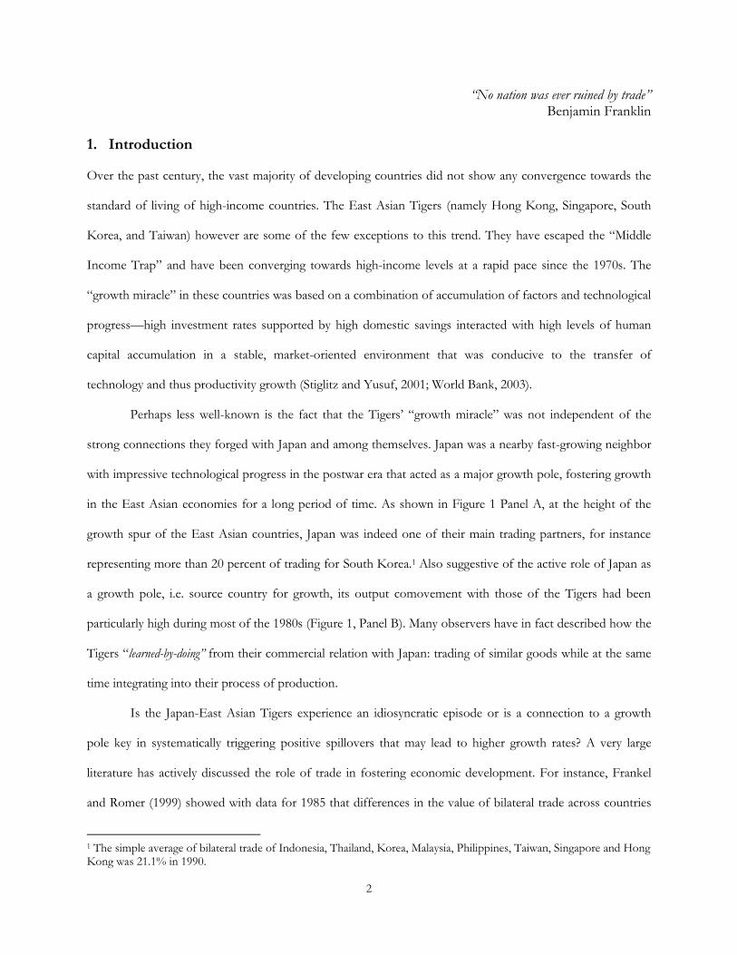
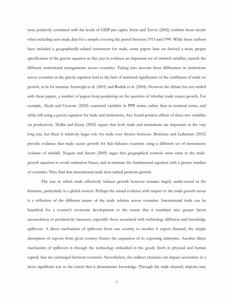
Figure 1. The Connection of Japan and the East Asian Countries

Notes: The graph on the left corresponds to the output correlation between East Asian Tigers and Japan. The graph on the right presents the main trade partners of the Tigers for 1990. The sample of UE15 includes: Austria, Belgium, Denmark, Finland, France, Germany, Greece, Ireland, Italy, Luxembourg, Netherlands, Portugal , Spain, Sweden and the United Kingdom; the sample of EAP countries includes Hong Kong, Indonesia, Korea Rep., Malaysia, Philippines, Singapore, Taiwan and Thailand. Sources: WITS and WDI.

0%

10%

20%

30%

40%

50%

60%

70%

80%

90%

100%

Indonesia Thailand Korea Malaysia Philippines Taiwan Singapore HongKong

% o

f T

ota

l T

rad

e1990

World

UE15

USA

EAP

JPN

-0.4

-0.2

0

0.2

0.4

0.6

0.8

1

1975

1976

1977

1978

1979

1980

1981

1982

1983

1984

1985

1986

1987

1988

1989

1990

1991

1992

1993

1994

1995

1996

1997

1998

1999

2000

Output Co-Movement Between EAP and Japan

15-year rolling correlation of the Real GDP Growth

HKG KOR IDN

MYS THA SGP

2005

With zeros included

(1) (2) (3) (4)

ln(distance) -0.85*** -1.14*** -1.185*** -2.173***(0.04) (0.03) (0.04) (0.0484)

ln (population) -0.24 -0.14 -0.0884*** 0.624***(0.03) 0.02 (0.02) (0.0301)

ln(population_partner) 0.61** 0.96** 1.041*** 1.729***(0.03) 0.02 (0.02) (0.0301)

ln(area) -0.12 -0.16 -0.143*** -0.276***(0.02) (0.02) (0.02) (0.0241)

ln(area_partner) -0.19* -0.23* -0.235*** -0.460***(0.02) (0.02) (0.02) (0.0241)

Landlock -0.36 -0.81* -0.728*** -1.790***(0.08) (0.06) (0.06) (0.0645)

Border 5.10 0.39 0.72 7.390*(1.78) (1.37) (2.56) (4.067)

Border*ln(distance) 0.15 0.60 0.979** 2.033***(0.30) (0.29) (0.43) (0.568)

Borber*ln(population) -0.29 -0.21 -0.17 -0.508**(0.18) (0.15) (0.15) (0.241)

Borber*ln(population_partner) -0.14 -0.22 -0.24 -0.639***(0.18) (0.14) (0.15) (0.241)

Border*ln(area) -0.06 -0.03 -0.05 -0.316(0.15) (0.15) (0.18) (0.261)

Border*ln(area_partner) -0.07 0.00 -0.06 -0.0971(0.15) (0.16) (0.18) (0.261)

Border*Landlock 0.33 1.05 0.378 1.482***(0.33) (0.20) (0.24) (0.345)

Observations 3220 8906 9108 19,100

R-squared 0.36 0.35 0.384 0.295

1985

Without zeros included

Notes : The dependant variable is openess. All regressions include a constant. Standard deviations are in parentheses. ***significant at 1 percent; **5

percent; * 10 percent.

Table 1. The Bilateral Equation

29

Partner: Main Partner Main World Growth Pole

(1) (2)

Openess 3.090** 3.071**(1.382) (1.412)

ln(population) 0.155 0.197*(0.105) (0.108)

ln(area) 0.000658 -0.0147(0.117) (0.116)

Share of Trade - with partner -4.829*** 2.461*(1.391) (1.401)

European Languages 2.047*** 1.492***(0.336) (0.360)

Number of Countries 151 151

Notes: The dependant variable is the logarithm of GDP per worker. All regressions include a constant. Standard

deviations are in parentheses. ***significant at 1 percent; **5 percent; * 10 percent.

Table 2. Benchmarks

Partner:

(1) (2) (3) (4) (5) (6)

Openess 2.759* 2.325 2.433* 2.641* 1.732 1.926(1.495) (1.483) (1.429) (1.474) (1.416) (1.268)

ln(population) -0.0431 -0.0415 -0.0660 -0.0213 -0.0912 -0.0909(0.125) (0.112) (0.121) (0.128) (0.112) (0.114)

ln(area) 0.141 0.102 0.135 0.137 0.124 0.139(0.0987) (0.103) (0.0946) (0.0981) (0.0928) (0.0884)

Share of Trade - with partner -4.105*** -4.706*** -4.329*** 2.006 1.495 1.558(1.591) (1.408) (1.537) (1.315) (1.172) (1.213)

European Languages 1.676*** 1.648*** 1.613*** 1.162*** 0.977*** 1.003***(0.389) (0.359) (0.374) (0.368) (0.333) (0.327)

IIT - Overall 3.081** 1.762 3.222*** 1.156(1.315) (1.504) (1.248) (1.555)

IIT - with partner 2.982*** 1.756* 3.792*** 2.804**(0.944) (0.961) (0.933) (1.130)

Number of Countries 142 142 142 142 142 142

Main Partner Main World Growth Pole

Notes: Data reported are the results of a panel between 2000-2007. The dependant variable is the logarithm of GDP per capita. All regressions

include a constant. Standard deviations are in parentheses. ***significant at 1 percent; **5 percent; * 10 percent.

Table 3. The Industry Channel: Intra-Industry Trade

30

(1) (2) (3) (4) (5) (6)

Openess 3.073* 2.923** 2.935* 3.050* 2.832** 3.016**(1.644) (1.354) (1.635) (1.603) (1.222) (1.466)

ln(population) 0.265** 0.119 0.254* 0.343*** 0.235** 0.346***(0.132) (0.117) (0.134) (0.133) (0.116) (0.130)

ln(area) -0.0325 0.0199 -0.0305 -0.0601 -0.0271 -0.0669(0.132) (0.134) (0.128) (0.126) (0.125) (0.130)

Share of Trade - with partner -3.906** -4.741** -4.759*** 2.976* 3.826** 3.979**(1.668) (1.936) (1.816) (1.537) (1.577) (1.671)


Commodity product - Overall -2.559 -3.424 -2.776 -1.079(2.456) (3.468) (2.330) (2.829)

Commodity product - with partner 0.210 2.829 -6.974** -6.300(3.289) (5.071) (3.286) (4.650)

Upstreamness in Exports - Overall 3.320* 3.997** 4.061** 3.368*(1.969) (1.801) (1.933) (1.964)

Upstreamness in Exports - with partner 0.263 -1.272 2.810*** 0.849(1.155) (1.250) (0.997) (1.330)

Upstreamness in Imports - Overall -6.181 -7.138 -8.359** -8.143*(3.862) (4.584) (3.874) (4.215)

Upstreamness in Imports - with partner -0.519 0.404 -1.745 0.295(1.834) (2.004) (2.671) (2.934)


Table 4. The Industry Channel: Rank in the Channel Value of the Product

Main Partner Pole

Notes: Data reported are the results of a panel between 2000-2007. The dependant variable is the logarithm of GDP per capita. All regressions include a

constant. Standard deviations are in parentheses. ***significant at 1 percent; **5 percent; * 10 percent.

Partner:

(1) (2) (3) (4) (5) (6)

Openess 3.615** 3.362** 3.477*** 3.453** 3.382** 3.420**(1.422) (1.327) (1.333) (1.444) (1.383) (1.392)

ln(population) 0.0887 0.0981 0.0820 0.130 0.151 0.141(0.108) (0.106) (0.107) (0.110) (0.108) (0.109)

ln(area) 0.0768 0.0354 0.0626 0.0569 0.0461 0.0530(0.126) (0.121) (0.122) (0.124) (0.121) (0.122)

Share of Trade - with partner -4.997*** -4.516*** -4.759*** 1.506 1.570 1.422(1.596) (1.574) (1.588) (1.538) (1.508) (1.525)


Skilled-Labor Intensive Goods - Overall 9.134*** 5.477 8.854*** 3.382(2.287) (3.475) (2.385) (3.619)

Skilled-Labor Intensive Goods- with partner 5.877*** 3.028 6.893*** 5.065**(1.425) (2.315) (1.622) (2.543)



Notes: Data reported are the results of a panel between 2000-2007.The dependant variable is the logarithm of GDP per worker. All regressions include a


Table 5. Process of Production: Technological Intensity of Factors of Production

31

Partner:

(1) (2) (3) (4) (5) (6)

Openess 2.498 3.033* 1.797 2.390 2.642* 1.985(1.850) (1.576) (1.664) (1.836) (1.419) (2.110)

ln(population) -0.00593 0.129 -0.0942 0.0346 0.0818 -0.00339(0.168) (0.132) (0.156) (0.174) (0.127) (0.193)

ln(area) 0.0791 0.0160 0.0745 0.0640 0.0558 0.0629(0.0951) (0.108) (0.0862) (0.0954) (0.107) (0.0965)

Share of Trade - with partner -4.604*** -5.085*** -4.925*** 2.271* 2.906* 2.165(1.636) (1.716) (1.472) (1.335) (1.531) (1.407)


High Technological product - Overall 3.863 11.48*** 3.636 4.958(3.944) (4.000) (3.876) (6.763)

High Technological product - with partner -0.352 -6.114*** 2.153 -0.487(2.280) (1.825) (1.783) (3.067)



Table 6. Product Channel: Technological products



Partner:

(1) (2) (3) (4) (5) (6)

Openess 2.898 3.212** 2.845 2.799 2.888* 3.036(1.801) (1.544) (1.829) (1.774) (1.495) (1.902)

ln(population) 0.103 0.120 0.0992 0.136 0.134 0.140(0.111) (0.114) (0.113) (0.114) (0.111) (0.116)

ln(area) 0.0409 0.0349 0.0418 0.0309 0.0395 0.0398(0.126) (0.133) (0.124) (0.123) (0.126) (0.128)

Share of Trade - with partner -4.493*** -4.684*** -5.414*** 2.371 3.111* 3.305**(1.611) (1.779) (1.704) (1.552) (1.718) (1.683)


Commodity product - Overall -0.959 -2.588 -0.929 0.705(1.906) (3.173) (1.832) (2.715)

Commodity product - with partner 0.567 4.605 -4.089 -5.177(2.942) (5.228) (3.249) (4.896)



Table 7. Product Channel: Commodity Products



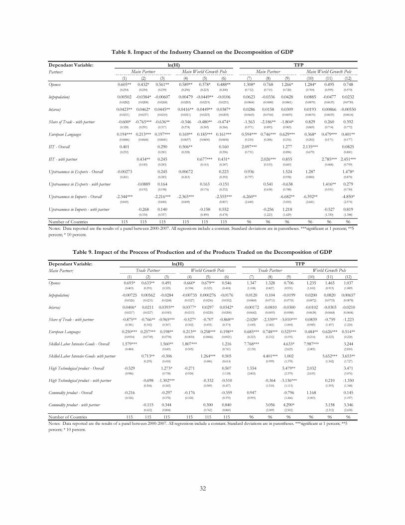
32

Dependant Variable:

Partner:

(1) (2) (3) (4) (5) (6) (7) (8) (9) (10) (11) (12)

Openess 0.605** 0.432* 0.561** 0.589** 0.378* 0.488** 1.308* 0.768 1.266* 1.284* 0.495 0.748(0.254) (0.254) (0.239) (0.250) (0.223) (0.200) (0.712) (0.715) (0.720) (0.704) (0.595) (0.570)

ln(population) 0.00502 -0.0384* -0.00607 0.00479 -0.0449** -0.0106 0.0623 -0.0336 0.0428 0.0885 -0.0477 0.0232(0.0282) (0.0208) (0.0268) (0.0283) (0.0219) (0.0251) (0.0864) (0.0680) (0.0861) (0.0870) (0.0635) (0.0750)

ln(area) 0.0423** 0.0462* 0.0445** 0.0416** 0.0449** 0.0387* 0.0286 0.0158 0.0309 0.0193 0.00866 -0.00550(0.0211) (0.0237) (0.0210) (0.0211) (0.0225) (0.0205) (0.0665) (0.0760) (0.0693) (0.0670) (0.0655) (0.0614)

Share of Trade - with partner -0.600* -0.765*** -0.636** -0.346 -0.480** -0.474* -1.563 -2.186** -1.804* 0.829 0.260 0.392(0.328) (0.291) (0.317) (0.278) (0.243) (0.266) (0.971) (0.893) (0.965) (0.869) (0.714) (0.772)

European Languages 0.194*** 0.213*** 0.197*** 0.169** 0.185*** 0.161*** 0.594*** 0.746*** 0.629*** 0.368* 0.479*** 0.401**(0.0686) (0.0668) (0.0681) (0.0657) (0.0600) (0.0606) (0.210) (0.206) (0.216) (0.202) (0.171) (0.177)

IIT - Overall 0.401 0.290 0.506** 0.160 2.097*** 1.277 2.135*** 0.0825(0.252) (0.281) (0.228) (0.296) (0.731) (0.896) (0.679) (0.881)

IIT - with partner 0.434** 0.245 0.677*** 0.431* 2.026*** 0.855 2.785*** 2.451***(0.185) (0.283) (0.161) (0.247) (0.533) (0.683) (0.468) (0.799)

Upstreamness in Exports - Overall -0.00273 0.245 0.00672 0.223 0.936 1.524 1.287 1.478*(0.261) (0.283) (0.263) (0.292) (0.797) (0.938) (0.800) (0.874)

Upstreamness in Exports - with partner -0.0889 0.164 0.163 -0.151 0.541 -0.638 1.416** 0.279(0.192) (0.198) (0.176) (0.232) (0.638) (0.788) (0.551) (0.750)

Upstreamness in Imports - Overall -2.344*** -2.216*** -2.365*** -2.555*** -6.260** -6.682** -6.592** -4.850*(0.845) (0.840) (0.849) (0.807) (2.640) (3.010) (2.681) (2.574)

Upstreamness in Imports - with partner -0.268 0.140 -0.158 0.552 -0.256 1.218 -0.527 0.819(0.334) (0.357) (0.490) (0.478) (1.223) (1.429) (1.330) (1.388)

Number of Countries 115 115 115 115 115 115 96 96 96 96 96 96

Notes: Data reported are the results of a panel between 2000-2007. All regressions include a constant. Standard deviations are in parentheses. ***significant at 1 percent; **5


Table 8. Impact of the Industry Channel on the Decomposition of GDP

ln(H) TFP

Main Partner Main World Growth Pole Main Partner Main World Growth Pole

Dependant Variable:

Main Partner:

(1) (2) (3) (4) (5) (6) (7) (8) (9) (10) (11) (12)

Openess 0.693* 0.633** 0.491 0.660* 0.679** 0.546 1.347 1.328 0.706 1.235 1.465 1.037(0.403) (0.291) (0.325) (0.394) (0.323) (0.418) (1.108) (0.827) (0.931) (1.102) (0.913) (1.089)

ln(population) -0.00725 0.00562 -0.0284 -0.00735 0.000276 -0.0176 0.0120 0.104 -0.0199 0.0200 0.0820 0.00657(0.0326) (0.0231) (0.0268) (0.0327) (0.0256) (0.0352) (0.0868) (0.0711) (0.0735) (0.0872) (0.0735) (0.0878)

ln(area) 0.0406* 0.0211 0.0393** 0.0377* 0.0297 0.0342* -0.00172 -0.0810 -0.0300 -0.0102 -0.0303 -0.0210(0.0217) (0.0227) (0.0183) (0.0213) (0.0220) (0.0200) (0.0642) (0.0693) (0.0580) (0.0638) (0.0668) (0.0606)

Share of Trade - with partner -0.875** -0.766** -0.965*** -0.527* -0.707 -0.868** -2.028* -2.339** -3.010*** 0.0839 -0.759 -1.223(0.381) (0.342) (0.307) (0.302) (0.451) (0.374) (1.045) (1.061) (1.004) (0.985) (1.457) (1.224)

European Languages 0.250*** 0.257*** 0.198** 0.213** 0.258*** 0.198** 0.685*** 0.748*** 0.525*** 0.484** 0.626*** 0.514**(0.0934) (0.0749) (0.0794) (0.0850) (0.0846) (0.0921) (0.223) (0.212) (0.195) (0.214) (0.225) (0.220)

Skilled-Labor Intensive Goods - Overall 1.579*** 1.560** 1.807*** 1.216 7.768*** 4.633* 7.987*** 3.244(0.484) (0.645) (0.505) (0.761) (2.130) (2.625) (2.405) (2.810)

Skilled-Labor Intensive Goods- with partner 0.713** -0.306 1.264*** 0.505 4.401*** 1.002 5.652*** 3.653**(0.295) (0.418) (0.406) (0.614) (0.999) (1.378) (1.502) (1.727)

High Technological product - Overall -0.529 1.273* -0.271 0.507 1.554 5.479** 2.032 3.471(0.986) (0.758) (0.924) (1.128) (2.802) (2.379) (2.655) (3.076)

High Technological product - with partner -0.698 -1.302*** -0.332 -0.510 -0.364 -3.136*** 0.210 -1.350(0.506) (0.365) (0.509) (0.437) (1.510) (1.113) (1.593) (1.348)

Commodity product - Overall -0.216 -0.297 -0.176 -0.359 0.947 -0.796 1.168 0.145(0.326) (0.378) (0.324) (0.370) (0.995) (1.266) (1.003) (1.197)

Commodity product - with partner -0.115 0.344 0.300 0.840 3.056 4.290* 3.158 3.346(0.652) (0.804) (0.762) (0.860) (2.009) (2.502) (2.312) (2.658)

Number of Countries 115 115 115 115 115 115 96 96 96 96 96 96

Notes: Data reported are the results of a panel between 2000-2007. All regressions include a constant. Standard deviations are in parentheses. ***significant at 1 percent; **5


Table 9. Impact of the Process of Production and of the Products Traded on the Decomposition of GDP

ln(H) TFP

Trade Partner World Growth Pole Trade Partner World Growth Pole

33

(1) (2) (3) (4)

Openess 4.038 3.780** 4.188** 4.181*(2.724) (1.711) (1.779) (2.280)

ln(population) 0.0421 0.421** 0.124 0.149(0.215) (0.171) (0.127) (0.194)

ln(area) 0.171 0.0118 0.148 0.160(0.130) (0.129) (0.147) (0.136)

Share of Trade - with developed countries 1.154*** 0.556 1.297*** 1.062**(0.435) (0.413) (0.412) (0.434)

Share of Trade - with emerging country 3.876 13.96*** 6.882 9.715*(4.904) (5.112) (5.048) (5.666)

European Languages -4.197 -2.607 -3.951 -4.611(3.367) (3.625) (2.715) (3.652)

Main Growth Pole = Developed Countries

IIT - with developed countries 3.349***(0.831)

Upstreamness in Exports - with developed countries 0.723(0.551)

Upstreamness in Imports - with developed countries -1.495(1.822)

Skilled-Labor Intensive Goods- with developed countries 7.554***(1.688)

Commodity product - with developed countries -14.58 -4.922(11.93) (11.06)

High Technological product - with developed countries 3.697*(2.112)

Main Growth Pole = Emerging Countries

IIT - with emerging countries -1.175(1.138)

Upstreamness in Exports - with emerging countries -0.161(0.243)

Upstreamness in Imports - with emerging countries -3.169***(0.755)

Skilled-Labor Intensive Goods - with emerging countries -2.851(1.831)

Commodity product - with emerging countries 4.214 2.109(8.669) (8.725)

High Technological product - with emerging countries -1.999(2.710)

Number of Countries 138 139 142 139

Table 10. World Growth Poles: Developed versus Emerging Countries

Notes: Data reported are the results of a panel between 2000-2007. The dependant variable is the logarithm of GDP per

capita. All regressions include a constant. Standard deviations are in parentheses. ***significant at 1 percent; **5 percent; * 10

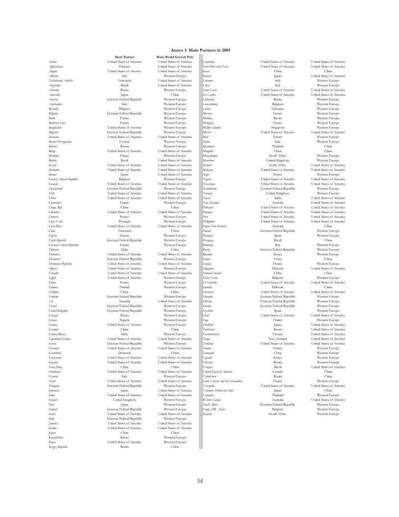
34


Aruba United States of America United States of America Cambodia United States of America United States of America

Afghanistan Pakistan United States of America Saint Kitts and Nevis United States of America United States of America

Angola United States of America United States of America Korea China China

Albania Italy Western Europe Kuwait Japan United States of America

Netherlands Antilles Venezuela United States of America Lebanon Italy Western Europe

Argentina Brazil United States of America Libya Italy Western Europe

Armenia Russia Western Europe Saint Lucia United States of America United States of America

Australia Japan China Sri Lanka United States of America United States of America

Austria German Federal Republic Western Europe Lithuania Russia Western Europe

Azerbaijan Italy Western Europe Luxembourg Belgium Western Europe

Burundi Belgium Western Europe Latvia Lithuania Western Europe

Belgium German Federal Republic Western Europe Morocco France Western Europe

Benin France Western Europe Moldova Russia Western Europe

Burkina Faso France Western Europe Malagasy France Western Europe

Bangladesh United States of America Western Europe Maldive Islands Singapore Western Europe

Bulgaria German Federal Republic Western Europe Mexico United States of America United States of America

Bahamas United States of America United States of America Mali France Western Europe

Bosnia-Herzegovina Croatia Western Europe Malta Italy Western Europe

Belarus Russia Western Europe Myanmar Thailand China

Belize United States of America United States of America Mongolia China China

Bermuda France Western Europe Mozambique South Africa Western Europe

Bolivia Brazil United States of America Mauritius United Kingdom Western Europe

Brazil United States of America United States of America Malawi South Africa United States of America

Barbados United States of America United States of America Malaysia United States of America United States of America

Brunei Japan United States of America Niger France Western Europe

Central African Republic Belgium Western Europe Nigeria United States of America United States of America

Canada United States of America United States of America Nicaragua United States of America United States of America

Switzerland German Federal Republic Western Europe Netherlands German Federal Republic Western Europe

Chile United States of America United States of America Norway United Kingdom Western Europe

China United States of America United States of America Nepal India United States of America

Cameroun France Western Europe New Zealand Australia United States of America

Congo, Rep. China China Pakistan United States of America United States of America

Colombia United States of America United States of America Panama United States of America United States of America

Comoros France Western Europe Peru United States of America United States of America

Cape Verde Portugal Western Europe Philippines United States of America United States of America

Costa Rica United States of America United States of America Papua New Guinea Australia China

Cuba Venezuela China Poland German Federal Republic Western Europe

Cyprus Greece Western Europe Portugal Spain Western Europe

Czech Republic German Federal Republic Western Europe Paraguay Brazil China

German Federal Republic France Western Europe Romania Italy Western Europe

Djibouti India China Russia German Federal Republic Western Europe

Dominica United States of America United States of America Rwanda Kenya Western Europe

Denmark German Federal Republic Western Europe Sudan China China

Dominican Republic United States of America United States of America Senegal France Western Europe

Algeria United States of America Western Europe Singapore Malaysia United States of America

Ecuador United States of America United States of America Solomon Islands China China

Egypt United States of America Western Europe Sierra Leone Belgium Western Europe

Spain France Western Europe El Salvador United States of America United States of America

Estonia Finland Western Europe Somalia Djibouti China

Ethiopia China China Suriname United States of America United States of America

Finland German Federal Republic Western Europe Slovakia German Federal Republic Western Europe

Fiji Australia United States of America Slovenia German Federal Republic Western Europe

France German Federal Republic Western Europe Sweden German Federal Republic Western Europe

United Kingdom German Federal Republic Western Europe Seychelles Spain Western Europe

Georgia Russia Western Europe Chad United States of America United States of America

Ghana Nigeria Western Europe Togo France Western Europe

Guinea United States of America Western Europe Thailand Japan United States of America

Gambia China China Tajikistan Russia United States of America

Guinea-Bissau India Western Europe Turkmenistan Ukraine United States of America

Equatorial Guinea United States of America United States of America Tonga New Zealand United States of America

Greece German Federal Republic Western Europe Trinidad United States of America United States of America

Grenada United States of America United States of America Tunisia France Western Europe

Greenland Denmark China Tanzania China Western Europe

Guatemala United States of America United States of America Uganda Kenya Western Europe

Guyana United States of America United States of America Ukraine Russia Western Europe

Hong Kong China China Uruguay Brazil United States of America

Honduras United States of America United States of America United States of America Canada China

Croatia Italy Western Europe Uzbekistan Russia China

Haiti United States of America United States of America Saint Vincent and the Grenadines France Western Europe

Hungary German Federal Republic Western Europe Venezuela United States of America United States of America

Indonesia Japan United States of America Vietnam, Democratic Rep. Japan China

India United States of America United States of America Vanuatu Thailand Western Europe

Ireland United Kingdom Western Europe Western Samoa Australia United States of America

Iran Japan Western Europe South Africa German Federal Republic Western Europe

Iceland German Federal Republic Western Europe Congo, DR - Zaire Belgium Western Europe

Israel United States of America United States of America Zambia South Africa Western Europe

Italy German Federal Republic Western Europe

Jamaica United States of America United States of America

Jordan United States of America United States of America

Japan China China

Kazakhstan Russia Western Europe

Kenya United States of America Western Europe

Kyrgyz Republic Russia China

Annex 1: Main Partners in 2005

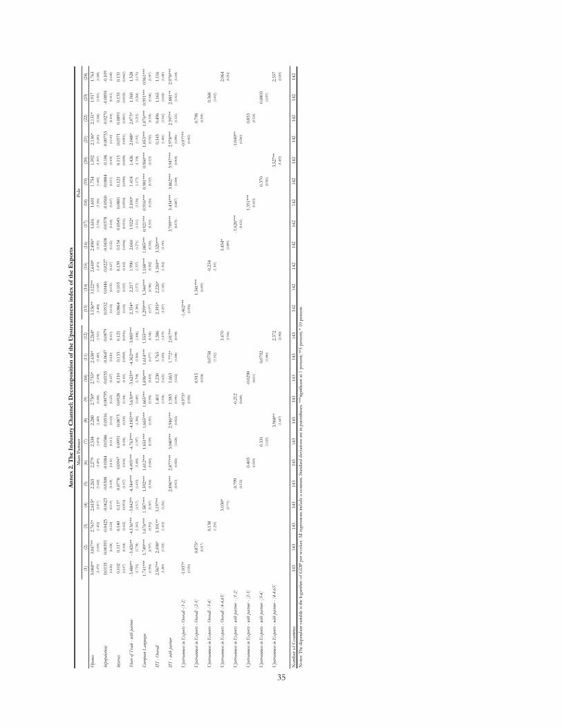
35

(1)

(2)

(3)

(4)

(5)

(6)

(7)

(8)

(9)

(10)

(11)

(12)

(13)

(14)

(15)

(16)

(17)

(18)

(19)

(20)

(21)

(22)

(23)

(24)

Ope

ness

3.0

84**

3.0

47**

2.7

61*

2.6

15*

2.2

65

2.2

79

2.3

38

2.2

80

2.7

50*

2.7

55*

2.4

38*

2.2

64*

3.1

36**

3.1

22**

2.6

40*

2.4

96*

1.6

16

1.6

01

1.7

54

1.5

92

2.1

36*

2.1

31*

1.9

17

1.7

63

(1.4

79)

(1.5

05)

(1.4

92)

(1.4

17)

(1.4

82)

(1.4

95)

(1.4

74)

(1.4

49)

(1.4

58)

(1.4

98)

(1.4

20)

(1.3

21)

(1.4

88)

(1.5

29)

(1.4

74)

(1.3

93)

(1.3

36)

(1.3

56)

(1.4

02)

(1.3

67)

(1.2

00)

(1.2

46)

(1.3

01)

(1.2

08)

ln(p

opul

atio

n)0.0

135

0.0

0391

-0.0

425

-0.0

623

-0.0

308

-0.0

384

-0.0

386

-0.0

516

-0.0

0795

-0.0

155

-0.0

647

-0.0

879

0.0

532

0.0

446

-0.0

227

-0.0

438

-0.0

378

-0.0

560

-0.0

884

-0.1

06

-0.0

0753

-0.0

270

-0.0

894

-0.1

09

(0.1

26)

(0.1

28)

(0.1

24)

(0.1

19)

(0.1

09)

(0.1

11)

(0.1

11)

(0.1

10)

(0.1

23)

(0.1

27)

(0.1

20)

(0.1

13)

(0.1

32)

(0.1

35)

(0.1

27)

(0.1

22)

(0.1

04)

(0.1

07)

(0.1

11)

(0.1

09)

(0.1

10)

(0.1

14)

(0.1

15)

(0.1

08)

ln(a

rea)

0.1

02

0.1

17

0.1

40

0.1

37

0.0

778

0.0

947

0.0

991

0.0

873

0.0

928

0.1

10

0.1

33

0.1

21

0.0

864

0.1

03

0.1

39

0.1

34

0.0

543

0.0

801

0.1

21

0.1

15

0.0

571

0.0

891

0.1

35

0.1

31

(0.1

07)

(0.1

04)

(0.1

02)

(0.0

954)

(0.1

07)

(0.1

04)

(0.1

06)

(0.1

00)

(0.1

04)

(0.1

01)

(0.0

989)

(0.0

916)

(0.1

06)

(0.1

03)

(0.1

02)

(0.0

946)

(0.0

916)

(0.0

904)

(0.0

948)

(0.0

898)

(0.0

901)

(0.0

891)

(0.0

920)

(0.0

863)

Sha

re o

f T

rade

- w

ith

part

ner

-3.4

80**

-3.4

26**

-4.1

36**

*-3

.842**

-4.3

44**

*-4

.495**

*-4

.763**

*-4

.185**

*-3

.630**

-3.6

25**

-4.3

62**

*-3

.885**

*2.3

54*

2.2

17

1.9

90

2.0

60

1.9

22*

2.1

00*

1.4

18

1.4

26

2.0

48*

2.0

73*

1.5

60

1.5

28

(1.7

35)

(1.7

38)

(1.5

43)

(1.5

17)

(1.4

53)

(1.4

58)

(1.3

97)

(1.3

86)

(1.6

89)

(1.7

08)

(1.5

04)

(1.4

86)

(1.3

80)

(1.3

73)

(1.3

37)

(1.2

71)

(1.1

11)

(1.1

38)

(1.1

73)

(1.1

38)

(1.1

91)

(1.2

15)

(1.2

64)

(1.1

70)

Eur

opea

n L

angu

ages

1.7

41**

*1.7

49**

*1.6

76**

*1.5

87**

*1.5

92**

*1.6

12**

*1.6

51**

*1.6

65**

*1.6

65**

*1.6

96**

*1.6

14**

*1.5

55**

*1.2

99**

*1.3

44**

*1.1

68**

*1.0

85**

*0.9

21**

*0.9

16**

*0.9

81**

*0.9

60**

*1.0

53**

*1.0

76**

*0.9

91**

*0.9

61**

*(0

.394

)(0

.397

)(0

.392

)(0

.367

)(0

.366

)(0

.368

)(0

.359

)(0

.351

)(0

.394

)(0

.405

)(0

.377

)(0

.346

)(0

.377

)(0

.386

)(0

.382

)(0

.348

)(0

.315

)(0

.320

)(0

.333

)(0

.323

)(0

.316

)(0

.330

)(0

.346

)(0

.307

)

IIT

- O

vera

ll2.5

67**

2.4

98*

3.1

01**

3.1

97**

1.4

01

1.2

30

1.7

65

1.5

86

2.3

95*

2.2

26*

3.1

84**

3.3

20**

*0.3

45

0.4

96

1.1

65

1.1

16

(1.2

89)

(1.3

25)

(1.4

12)

(1.2

54)

(1.5

34)

(1.6

21)

(1.6

58)

(1.4

70)

(1.2

57)

(1.3

25)

(1.3

62)

(1.1

90)

(1.4

81)

(1.5

41)

(1.6

04)

(1.4

80)

IIT

- w

ith

part

ner

2.8

96**

*2.8

77**

*3.0

40**

*2.9

46**

*1.5

83

1.6

63

1.7

72*

2.0

17**

3.7

09**

*3.4

34**

*3.8

62**

*3.9

47**

*2.9

78**

*2.5

97**

2.8

81**

2.9

78**

*(0

.913

)(0

.920

)(1

.020

)(0

.925

)(0

.990

)(1

.022

)(1

.044

)(0

.944

)(0

.870

)(0

.887

)(1

.004

)(0

.900

)(1

.098

)(1

.121

)(1

.161

)(1

.104

)

Ups

trea

mne

ss in

Ex

port

s -

Ove

rall

-[1-2

]-1

.037*

-0.9

75*

-1.4

62**

*-0

.977**

(0.5

30)

(0.5

58)

(0.5

06)

(0.4

92)

Ups

trea

mne

ss in

Ex

port

s -

Ove

rall

-[2-3

]0.8

75*

0.9

15

1.3

41**

*0.7

98

(0.5

17)

(0.5

58)

(0.4

95)

(0.5

09)

Ups

trea

mne

ss in

Ex

port

s -

Ove

rall

-[3-4

]0.1

38

0.0

758

-0.2

34

0.3

68

(1.2

50)

(1.3

12)

(1.3

01)

(1.4

02)

Ups

trea

mne

ss in

Ex

port

s -

Ove

rall

-[4-4

.65]

5.0

30*

3.4

70

5.4

54*

2.0

64

(2.7

71)

(3.3

56)

(2.8

09)

(4.2

51)

Ups

trea

mne

ss in

Ex

port

s -

with

part

ner

- [1

-2]

-0.7

99

-0.2

12

-1.6

26**

*-1

.040**

(0.5

32)

(0.6

08)

(0.4

21)

(0.5

00)

Ups

trea

mne

ss in

Ex

port

s -

with

part

ner

- [2

-3]

0.4

03

-0.0

290

1.3

51**

*0.8

53

(0.5

09)

(0.6

11)

(0.4

15)

(0.5

24)

Ups

trea

mne

ss in

Ex

port

s -

with

part

ner

-[3-4

]0.3

31

0.0

792

0.3

70

0.0

803

(1.0

23)

(1.0

80)

(0.9

02)

(1.0

57)

Ups

trea

mne

ss in

Ex

port

s -

with

part

ner

- [4

-4.6

5]

3.9

68**

2.3

72

3.5

27**

2.3

57

(1.6

47)

(2.0

84)

(1.4

83)

(2.6

03)

Num

ber

of

Co

untr

ies

143

143

143

143

143

143

143

143

143

143

143

143

142

142

142

142

142

142

142

142

142

142

142

142

Mai

n P

artn

erP

ole

An

nex

2.

Th

e I

nd

ust

ry C

han

nel:

Deco

mp

osi

tio

n o

f th

e U

pst

ream

ness

in

dex

of

the E

xp

ort

s

No

tes:

The

dep

end

ant

var

iab

le is

the

logar

ithm

of

GD

P p

er w

ork

er. A

ll re

gre

ssio

ns

incl

ud

e a

const

ant. S

tand

ard

dev

iatio

ns

are

in p

aren

thes

es. **

*sig

nif

ican

t at

1 p

erce

nt; *

*5 p

erce

nt; *

10 p

erce

nt.

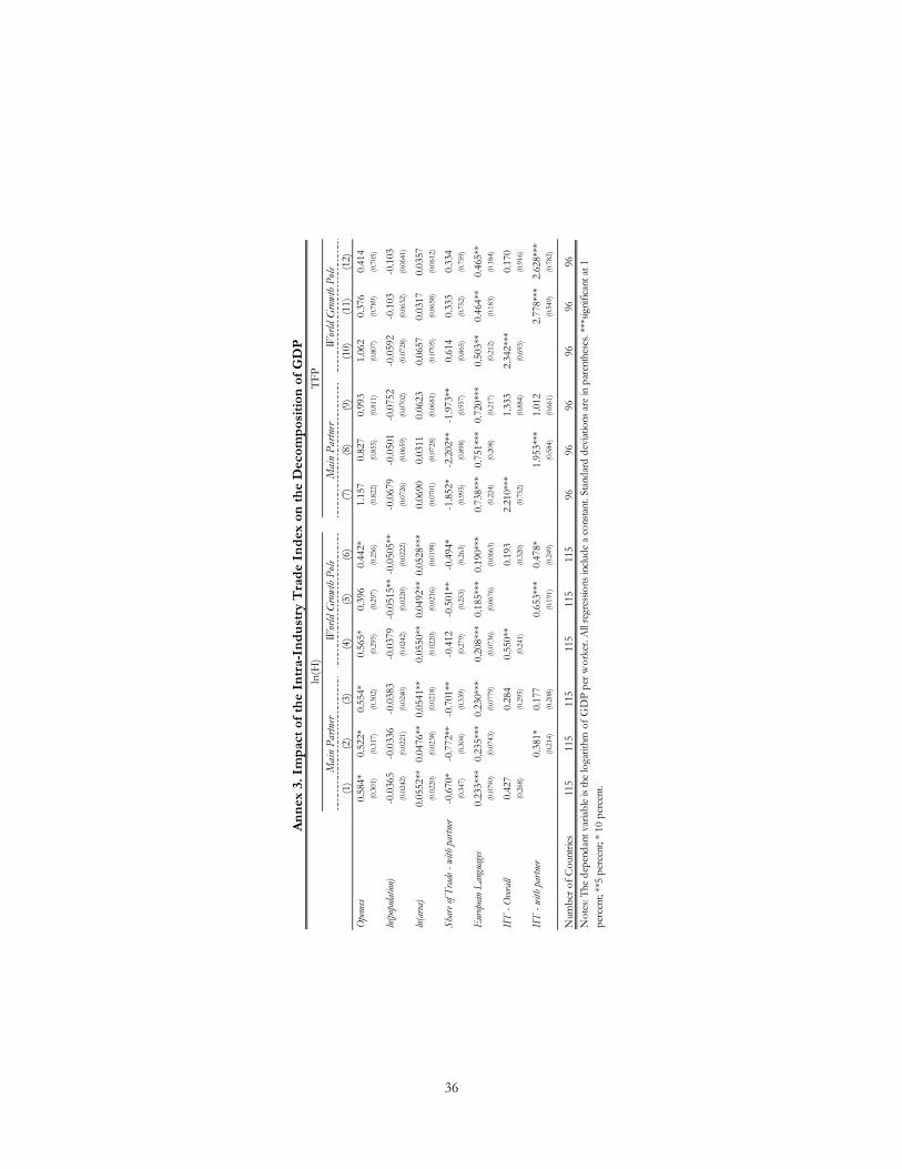
36

(1)

(2)

(3)

(4)

(5)

(6)

(7)

(8)

(9)

(10)

(11)

(12)

Ope

ness

0.5

84*

0.5

22*

0.5

54*

0.5

65*

0.3

96

0.4

42*

1.1

57

0.8

27

0.9

93

1.0

62

0.3

76

0.4

14

(0.3

01)

(0.3

17)

(0.3

02)

(0.2

95)

(0.2

97)

(0.2

56)

(0.8

22)

(0.8

55)

(0.8

11)

(0.8

07)

(0.7

89)

(0.7

05)

ln(p

opul

atio

n)-0

.0365

-0.0

336

-0.0

383

-0.0

379

-0.0

515**

-0.0

505**

-0.0

679

-0.0

501

-0.0

752

-0.0

592

-0.1

03

-0.1

03

(0.0

242)

(0.0

221)

(0.0

240)

(0.0

242)

(0.0

220)

(0.0

222)

(0.0

726)

(0.0

659)

(0.0

702)

(0.0

728)

(0.0

632)

(0.0

641)

ln(a

rea)

0.0

552**

0.0

476**

0.0

541**

0.0

550**

0.0

492**

0.0

528**

*0.0

690

0.0

311

0.0

623

0.0

657

0.0

317

0.0

357

(0.0

220)

(0.0

238)

(0.0

218)

(0.0

220)

(0.0

216)

(0.0

198)

(0.0

701)

(0.0

728)

(0.0

681)

(0.0

705)

(0.0

658)

(0.0

612)

Sha

re o

f T

rade

- w

ith

part

ner

-0.6

70*

-0.7

72**

-0.7

01**

-0.4

12

-0.5

01**

-0.4

94*

-1.8

52*

-2.2

02**

-1.9

73**

0.6

14

0.3

33

0.3

34

(0.3

47)

(0.3

04)

(0.3

39)

(0.2

79)

(0.2

53)

(0.2

63)

(0.9

95)

(0.8

98)

(0.9

57)

(0.8

65)

(0.7

52)

(0.7

59)

Eur

opea

n L

angu

ages

0.2

33**

*0.2

35**

*0.2

30**

*0.2

08**

*0.1

85**

*0.1

90**

*0.7

38**

*0.7

51**

*0.7

20**

*0.5

03**

0.4

64**

0.4

65**

(0.0

790)

(0.0

743)

(0.0

779)

(0.0

736)

(0.0

676)

(0.0

663)

(0.2

24)

(0.2

08)

(0.2

17)

(0.2

12)

(0.1

83)

(0.1

84)

IIT

- O

vera

ll0.4

27

0.2

84

0.5

50**

0.1

93

2.2

10**

*1.3

33

2.3

42**

*0.1

70

(0.2

68)

(0.2

95)

(0.2

41)

(0.3

20)

(0.7

52)

(0.8

84)

(0.6

93)

(0.9

16)

IIT

- w

ith

part

ner

0.3

81*

0.1

77

0.6

53**

*0.4

78*

1.9

53**

*1.0

12

2.7

78**

*2.6

28**

*(0

.214

)(0

.208

)(0

.191

)(0

.249

)(0

.584

)(0

.661

)(0

.549

)(0

.782

)

Num

ber

of

Co

untr

ies

115

115

115

115

115

115

96

96

96

96

96

96

An

nex

3.

Imp

act

of

the I

ntr

a-I

nd

ust

ry T

rad

e I

nd

ex

on

th

e D

eco

mp

osi

tio

n o

f G

DP

No

tes:

The

dep

end

ant

var

iab

le is

the

logar

ithm

of

GD

P p

er w

ork

er. A

ll re

gre

ssio

ns

incl

ud

e a

const

ant. S

tand

ard

dev

iatio

ns

are

in p

aren

thes

es. **

*sig

nif

ican

t at

1

per

cent; *

*5 p

erce

nt; *

10 p

erce

nt.

ln(H

)T

FP

Mai

n P

artn

erW

orld

Gro

wth

Pol

eM

ain

Par

tner

Wor

ld G

row

th P

ole

how does trade cause growth? - gtap · 2013-03-19 · 1 how does trade cause growth? tatiana didier...

Documents