housework, fixed effects, and wages of married …stratton...housework, fixed effects, and wages of...

http://www.jstor.org

Housework, Fixed Effects, and Wages of Married WorkersAuthor(s): Joni Hersch and Leslie S. StrattonSource: The Journal of Human Resources, Vol. 32, No. 2, (Spring, 1997), pp. 285-307Published by: University of Wisconsin PressStable URL: http://www.jstor.org/stable/146216Accessed: 18/07/2008 17:13

Your use of the JSTOR archive indicates your acceptance of JSTOR's Terms and Conditions of Use, available at

http://www.jstor.org/page/info/about/policies/terms.jsp. JSTOR's Terms and Conditions of Use provides, in part, that unless

you have obtained prior permission, you may not download an entire issue of a journal or multiple copies of articles, and you

may use content in the JSTOR archive only for your personal, non-commercial use.

Please contact the publisher regarding any further use of this work. Publisher contact information may be obtained at

http://www.jstor.org/action/showPublisher?publisherCode=uwisc.

Each copy of any part of a JSTOR transmission must contain the same copyright notice that appears on the screen or printed

page of such transmission.

JSTOR is a not-for-profit organization founded in 1995 to build trusted digital archives for scholarship. We work with the

scholarly community to preserve their work and the materials they rely upon, and to build a common research platform that

promotes the discovery and use of these resources. For more information about JSTOR, please contact [email protected].

http://www.jstor.org/stable/146216?origin=JSTOR-pdf

http://www.jstor.org/page/info/about/policies/terms.jsp

http://www.jstor.org/action/showPublisher?publisherCode=uwisc

Housework, Fixed Effects, and Wages of Married Workers

Joni Hersch Leslie S. Stratton

ABSTRACT

Although the primacy of household responsibilities in determining gender differences in labor market outcomes is universally recognized, there has been little investigation of the direct effect of housework on wages. Using data from the Panel Study of Income Dynamics, cross-sectional wage regressions reveal a substantial negative relation between wages and housework for wives, which persists in specifications controlling for individual fixed effects. The evidence for husbands is inconclusive. Mar- ried women's housework time is, on average, three times that of married men's. The addition of housework time to the wage equations increases the explained component of the gender wage gap from 27-30 percent to 38 percent.

I. Introduction

The importance of housework in people's lives is far greater than economists' attention to it. Robert Eisner (1988) estimates the value of home production to be about one-third of conventional Gross National Product. Gender differences in housework time suggest that much of this output is produced by women. Even women employed full-time spend 20-30 hours per week on housework; employed men spend at most half that amount of time.1 While household

Joni Hersch is a professor of economics at the University of Wyoming in Laramie. Leslie S. Stratton is an assistant professor of economics at the University of Arizona in Tucson. Partial funding for Hersch was provided by NSF Grant #HRD-9250117. The authors thank the referees, Ron Oaxaca, Tony Tam, and participants at the 1995 WEA meeting and the 1994 National Bureau of Economic Re- search Summer Institute for their helpful comments. The data used in this article can be obtained beginning in August 1997 through July 2000 from Joni Hersch, Department of Economics, University of Wyoming, Laramie WY 82071. [Submitted March 1995; accepted August 1996] 1. See for example Hill (1985), Gronau (1977), and Juster and Stafford (1991).

THE JOURNAL OF HUMAN RESOURCES * XXXII * 2

286 The Journal of Human Resources

responsibilities have long been believed to affect wages via their effect on human capital accumulation, the sheer magnitude of housework time suggests that household responsibilities may have an additional, more direct effect on wages.2 The limited empirical evidence, based on cross-sectional data, does find an inverse relation between housework and wages for women.3 In this paper, we explore the empirical plausibility of different hypotheses that might account for this phe- nomenon, paying particular attention to endogeneity and omitted individual characteristics.

The only formal model linking home production and wages is that proposed by Gary Becker (1985). In his model, individual effort is limited and must be allocated across all activities. Effort expended on housework necessarily reduces the amount of effort available for market work. If work effort and wages are positively correlated, the wages of workers bearing greater household responsibilities will be lower than the wages of their less burdened counterparts, even if their human capital characteristics and labor market experience are identical.

Becker's effort model is predicated on the presence of a housework effect that directly lowers wages. An alternative explanation for the observed housework effect is that, rather than affecting wages directly, housework is correlated with unobserved individual characteristics that have a negative effect on wages. Esti- mation using instrumental variables and fixed effects models will enable us to disentangle these influences. If a direct mechanism is responsible, housework time will remain negatively related to wages after controlling for endogeneity and individual-specific characteristics. If unobserved characteristics are the determining factor, the observed negative correlation between wages and housework is spurious and will disappear when the wage-housework relation is correctly spec- ified.

In this paper, we estimate ordinary least squares (OLS), instrumental variables (IV), and fixed effects wage equations using panel data on married workers from the Panel Study of Income Dynamics. Our cross-sectional estimates-both OLS and IV-reveal a remarkably robust negative relation between wages and housework for wives. Fixed effects estimates reduce, but do not eliminate, this negative relation. For husbands, the relation is more tenuous. Ordinary least squares estimates suggest a negative relation between housework and wages, but the effect is statistically insignificant in the instrumental variables and fixed effects specifications. Overall, these results provide strong evidence for wives only that housework has a negative effect on earnings that is neither due solely to unobserved characteristics nor due to observable human capital measures. Given the substantial differences in housework time by gender, the contribution of time spent on housework to explaining the gender wage gap is considerable: the addition of housework time to the wage equation increases the explanatory power of observable characteristics from 27-30 percent to 38 percent.

2. This point has been made by a wide range of economists, including Becker (1991, 1985), Fuchs (1988), Oi (1993), and the Committee on Women's Employment and Related Social Issues (1986), as well as by numerous journalists. 3. See Coverman (1983), Hersch (1991a, 1991b), and Shelton and Firestone (1988).

Hersch and Stratton 287

II. Empirical Specification

Since our primary interest in this paper is in exploring the effect household activities may have upon wages, our focus is on estimating wage equations. We employ the standard empirical wage specification, modified to incorpo- rate information on household activities and an individual-specific component. Thus, we specify a wage equation of the following general form:

(1) ln Wi, = Xit P1 + 2 HWit + uit

(2) uit = i + Eit,

where Wi, is the real hourly wage of individual i at time t, Xi is a vector of measurable characteristics expected to affect wages (such as education and years of work experience), HWi, is time spent on household activities, and uit is the error term. The error term has two components: ii, which represents unobserved characteristics of individual i that affect wages in a fixed manner over time, and e,i, which represents random error, assumed to be normally distributed. If housework time has a direct negative effect on wages, as suggested by Becker's model, we expect P2 < 0.

If housework is correlated with uit, OLS estimates of P2 will be biased. This correlation could arise for at least two reasons. First, housework may be determined endogenously with the wage. The opportunity cost of time spent on home production is higher for those receiving higher market wages. Thus, those workers may be more likely to substitute market purchases for home production, which may reduce their time spent on housework. If so, then observed housework time could be correlated with both components of uit, and OLS estimates of J2 will be biased down: housework will appear to have a greater negative impact on wages than it actually does.

Second, the correlation between housework and the error term could be limited to the individual fixed effects component Li. One interpretation of Ji is as a measure of the individual's innate market productivity. If workers with higher levels of innate market productivity specialize more in market production and spend less time on housework, then [Li and housework time will be negatively correlated. Again, the coefficient on housework in a cross-sectional wage equation will be biased down.

Several empirical procedures are available to eliminate the bias that may arise due to a correlation of u, with housework time. Instrumental variables techniques can be used to construct an instrument for housework time and so yield consistent estimates of 12 no matter the nature of the correlation. If the correlation is restricted to the individual-specific component Ri, fixed effects estimation is the preferred procedure.

III. Data

The data set used in this analysis is the University of Michigan's Panel Study of Income Dynamics (PSID). This data set contains information on


a wide range of worker characteristics for a national sample of households, surveyed annually beginning in 1968. For our purposes, the most important characteristics of the survey are that it includes a measure of time spent on housework and that it provides the panel data necessary to estimate a fixed effects model.

Our analysis uses data from the years 1979 through 1987. We begin with 1979 because hourly wage data for wives are not consistently available until that year. We exclude observations from 1982 when housework data are not available. The sample is restricted to a relatively homogeneous population of white, married individuals, aged 20-64. All monetary values are normalized to 1987 dollars using the Consumer Price Index. For those individuals who are employed, we impose a lower real wage limit of $2.00 per hour in order to eliminate obviously miscoded responses.4 The small number of observations (18 total) in which an employed individual reported 70 or more hours of housework per week are also dropped due to possible miscoding (though all of the following analyses are unaffected by inclusion of these individuals).

Two samples are relevant. In the pooled cross-section estimates, we require complete information on all the variables used to estimate the wage equations (including variables to correct for possible selection bias for women and to instrument for housework in the wage equation). This yields observations on 11,444 job years for 2,250 men and on 6,971 job years for 1,734 women. Since multiple observations are required to estimate fixed effects models, sample observations for the fixed effects specifications are limited to those who are in the sample for at least two years. We again require complete information on all the variables used to estimate the wage equations. However, information on the instruments is not required; thus the fixed effects samples include observations not available in the pooled cross-section sample. These restrictions yield a fixed effects sample of 11,474 observations on 2,077 men and 6,803 observations on 1,473 women.

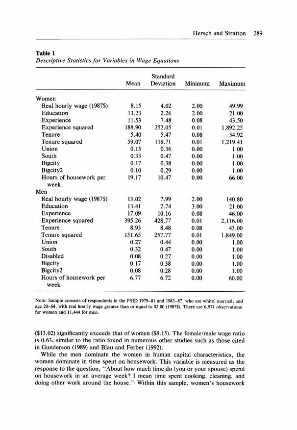
Descriptive statistics for the human capital and job-related variables included in the pooled cross-sectional log wage regressions are presented in Table 1. Variable summaries for the fixed effects sample are similar. Most of the variables are standard and require no discussion. Residence in a standard metropolitan statistical area (SMSA) with a population over 500,000 is represented by two dummy variables due to noncomparable measurement changes in 1983.5 Disability status is available for men for all years, but is available for wives only after 1980. Analyses including disability status for women indicate it had no significant effect on wages. We therefore exclude this variable from the analysis for women rather than reduce the sample to include only years for which this variable is available.

Relative to the women in the sample, on average the men have substantially more labor market experience and tenure.6 The average hourly real wage of men

4. In a few cases, the reported wage for a respondent was incongruously higher in one year than any other wage reported for the respondent. We eliminated the observations for the anomalous years, since these appear to be miscodes. 5. Though technically the definition of this variable does not change, 1970 census information was used to determine city size prior to 1983, while 1980 census information was used beginning in 1983. 6. Since we use panel data, it is important that time-dependent variables increment correctly. We thank Will Carrington and Kristin McCue for providing a SAS program to increment tenure and experience consistently.


Table 1 Descriptive Statistics for Variables in Wage Equations

Standard Mean Deviation Minimum Maximum

Women Real hourly wage (1987$) 8.15 4.02 2.00 49.99 Education 13.23 2.26 2.00 21.00 Experience 11.53 7.48 0.08 43.50 Experience squared 188.90 252.05 0.01 1,892.25 Tenure 5.40 5.47 0.08 34.92 Tenure squared 59.07 118.71 0.01 1,219.41 Union 0.15 0.36 0.00 1.00 South 0.33 0.47 0.00 1.00 Bigcity 0.17 0.38 0.00 1.00 Bigcity2 0.10 0.29 0.00 1.00 Hours of housework per 19.17 10.47 0.00 66.00

week Men

Real hourly wage (1987$) 13.02 7.99 2.00 140.80 Education 13.41 2.74 3.00 21.00 Experience 17.09 10.16 0.08 46.00 Experience squared 395.26 428.77 0.01 2,116.00 Tenure 8.93 8.48 0.08 43.00 Tenure squared 151.65 257.77 0.01 1,849.00 Union 0.27 0.44 0.00 1.00 South 0.32 0.47 0.00 1.00 Disabled 0.08 0.27 0.00 1.00 Bigcity 0.17 0.38 0.00 1.00 Bigcity2 0.08 0.28 0.00 1.00 Hours of housework per 6.77 6.72 0.00 60.00

week

Note: Sample consists of respondents in the PSID 1979-81 and 1983-87, who are white, married, and age 20-64, with real hourly wage greater than or equal to $2.00 (1987$). There are 6,971 observations for women and 11,444 for men.

($13.02) significantly exceeds that of women ($8.15). The female/male wage ratio is 0.63, similar to the ratio found in numerous other studies such as those cited in Gunderson (1989) and Blau and Ferber (1992).

While the men dominate the women in human capital characteristics, the women dominate in time spent on housework. This variable is measured as the response to the question, "About how much time do (you or your spouse) spend on housework in an average week? I mean time spent cooking, cleaning, and doing other work around the house." Within this sample, women's housework


time (19.2 hours) averages nearly three times that of men's (6.8 hours).7 For women, housework takes up more than half as much time as paid employment.

Yet, total home production time may be underreported in the PSID. Hill (1985) reports that the full-time employed married women surveyed in the 1975-76 Time Use Study averaged 24.58 hours per week on home-oriented work and that the full-time employed married men averaged 12.70 hours per week. While we would like to have more complete data, a further comparison with the Time Use Study does help to identify the most likely omissions and their relative magnitudes for men and women.

First, it is important to note that the largest category of household-related time (house and yard work) seems to have been captured within the PSID. Breaking down the total home production time of married workers by activity, the Time Use Study indicates that female full-time workers spend 66 percent of their home production time on house and yard work, 23 percent on services and shopping, and 11 percent on child care. For men, 57 percent of the time is spent on house/ yard work, 30 percent on services and shopping, and 13 percent on child care.8

Second, we expect that much of the additional work created by children, such as extra laundry, cooking, and cleaning, is subsumed in the reported total time spent on housework. It is very unlikely that respondents deducted from total time spent on housework that fraction made necessary by their children. Indeed, the presence of children adds five hours per week on average to the housework time of women (21.1 per week for those with children versus 16.3 for those without).9 The types of child care activities least likely to be included in reported time spent on housework are activities such as playing and reading, which may be more accurately labeled as leisure. Thus, we believe that the incremental amount of housework generated by child care is largely captured by the available data. The most likely omission is services/shopping activities, which seem to be relatively more important for men.

Of course, the impact any underreporting of housework time has on the estimated coefficients pertaining to housework depends on the correlation between the omitted activities and reported housework time, on the nature of the relation between the omitted activities and wages (specifically, whether this relation is similar to the relation between the reported activities and wages), and on the severity of general measurement error. As we discuss later, different measures of household activities may explain the disparity between the OLS results obtained here for men and those reported in other studies.

7. For all years in the sample but 1985, the husband responded to all questions about his wife as well as about himself. The wives self-reported their information only in 1985. The differences in average housework time between 1985 and the two adjacent years are trivial. This suggests that misreporting of wives' time by their husbands is not a significant problem. 8. The breakdown by activity for full-time employed married men and women is: house/yard work, 7.22 and 16.12; child care, 1.69 and 2.83; services/shopping, 3.79 and 5.63. See also Gronau (1977) and Juster and Stafford (1991). 9. This is similar in magnitude to the marginal time costs of children reported in Browning (1992, Ta- ble 4).


IV. Results

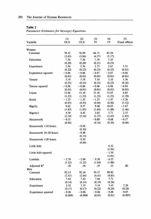
Table 2 presents OLS, IV, and fixed effects estimates of Wage Equation (1). The results for women are reported in Panel A, and for men in Panel B. The basic specification is a regression of the log of hourly wage on housework, education, experience and its square, tenure and its square, and dummy variables for union membership, residence in the South, city size, and, for men, disability status. Dummy variables for the OLS and IV for each year are also included. Alternative specifications reported in Table 2 include nonlinear housework effects and children. For women, the cross-sectional results are corrected for possible sample selection bias; however, the results without the sample selection correction are essentially identical.10 For convenience, all wage regression coefficients are multiplied by 100. OLS estimates of Equation (1) are reported in Columns 1 and 2, followed by IV estimates in Columns 3 and 4. Finally, we provide fixed effects estimates in Column 5.

A. Ordinary Least Squares Results

The estimated coefficients on the standard wage equation variables are consistent with those typically found in the literature. Wages increase with years of education, and with tenure and experience at decreasing rates. Workers covered by a union contract and residents of large cities earn significantly more on average; workers in the South and, for men, disabled workers earn less.

The primary concern here is the impact housework time has upon wages. The results indicate that housework has a significant negative effect on wages for both men and women. However, the magnitude of the effect is nearly twice as great for women (-0.547) as for men (-0.282), and this difference is statistically significant at the 1 percent level (t = 3.87). These findings raise two distinct concerns: why does time spent on housework appear to affect women's wages so much more than men's wages, and why do we find that housework time has any impact on men's wages when some other researchers find no such effect?

To address the large disparity in the coefficient estimates by gender, we estimated nonlinear specifications of the wage equation. Because men have a lower average level of housework than do women, if the wage-housework relation is concave, a linear equation will yield a smaller coefficient on housework for men than for women. To test this hypothesis, we estimate equations including both housework and its square. The results indicate no evidence of a nonlinear relation for men. The coefficient of the linear housework term remains negative and of a similar magnitude to that reported in Column 1, while the housework squared term is insignificant (t = 0.3). For women, the relation appears to be slightly convex, with a negative coefficient on the linear term and a small, but significantly

10. The variables used to control for selection bias include all the variables in the wage equation not related to current employment or housework-that is, education, age, experience, and dummy variables for residence in the South and in a large city-as well as the variables used to construct instruments for housework presented in Appendix A. Results were not sensitive to alternative specifications of the selection equation. The estimated selection equations are available upon request.


Table 2 Parameter Estimates for In(wage) Equations

(1) (2) (3) (4) (5) Variable OLS OLS IV IV Fixed effects

Women ... ..

Women Constant

Education

Experience

Experience squared

Tenure

Tenure squared

Union

South

Bigcity

Bigcity2

Housework

Housework <10 hours

Housework 10-20 hours

Housework >20 hours

Little kids

Little kids squared

Lambda

Adjusted R2 Men

Constant

Education

Experience

Experience squared

78.52 76.99 84.71 82.29 (3.63) (3.84) (4.57) (5.17) 7.56 7.56 7.39 7.35

(0.20) (0.20) (0.21) (0.23) 2.56 2.56 2.73 2.67 3.33

(0.22) (0.22) (0.23) (0.25) (0.63) -0.06 -0.06 -0.07 -0.07 -0.04 (0.01) (0.01) (0.01) (0.01) (0.01) 3.19 3.19 3.16 3.10 1.56

(0.23) (0.23) (0.23) (0.23) (0.26) -0.06 -0.06 -0.06 -0.06 -0.04 (0.01) (0.01) (0.01) (0.01) (0.01) 13.06 13.10 13.16 13.03 6.85 (1.23) (1.23) (1.23) (1.25) (1.39)

- 1.33 - 1.35 - 1.23 - 1.47 -5.26 (0.93) (0.93) (0.94) (0.96) (3.12) 9.62 9.57 9.48 10.05 - 1.67

(1.83) (1.83) (1.84) (1.88) (1.46) 4.50 4.45 3.83 3.71 2.15

(2.34) (2.34) (2.37) (2.43) (1.83) -0.55 -0.89 -0.68 -0.17 (0.04) (0.16) (0.20) (0.04)

-0.04 (0.30)

-0.48 (0.13)

-0.50 (0.06)

6.32 (1.94)

-1.50 (1.01)

-2.70 -2.68 -0.38 -4.25 (1.32) (1.32) (1.69) (1.88)

.36 .36 .35 .33 .80

92.13 92.16 93.17 89.83 (2.61) (2.64) (4.41) (9.83) 7.63 7.63 7.66 7.71

(0.14) (0.14) (0.19) (0.26) 3.35 3.35 3.34 3.42 2.26

(0.17) (0.17) (0.22) (0.24) (0.20) -0.06 -0.06 -0.06 -0.06 -0.05 (0.004) (0.004) (0.01) (0.01) (0.005)


Table 2 (continued)

(1) (2) (3) (4) (5) Variable OLS OLS IV IV Fixed effects

Tenure

Tenure squared

Union

South

Disabled

Bigcity

Bigcity2

Housework

Housework <10 hours

Housework 10-20 hours

Housework :20 hours

Little kids

Little kids squared

Adjusted R2

1.82 (0.14)

-0.02 (0.005) 10.50 (0.85)

-4.86 (0.79)

-12.69 (1.36) 13.99 (1.45)

-0.48 (1.95)

-0.28 (0.05)

1.82 (0.14)

-0.02 (0.005) 10.50 (0.85)

-4.87 (0.79)

-12.72 (1.36) 14.02 (1.45)

-0.52 (1.95)

1.82 (0.18)

-0.02 (0.01) 10.52 (1.11)

-5.02 (1.08)

-12.67 (1.77) 14.07 (1.88)

-0.50 (2.49)

-0.44 (0.41)

1.83 (0.20)

-0.02 (0.01) 10.31 (1.22)

-4.96 (1.62)

-12.62 (1.91) 14.40 (2.15)

-0.96 (2.68)

-0.56 (1.43)

-0.26 (0.17)

-0.35 (0.08)

-0.25 (0.06)

4.36 (2.38)

-0.49 (0.89)

.36 .36 .35 .36

Note: All coefficients are multiplied by 100. Standard errors in parentheses. The OLS and IV equations also include dummy variables for each year.

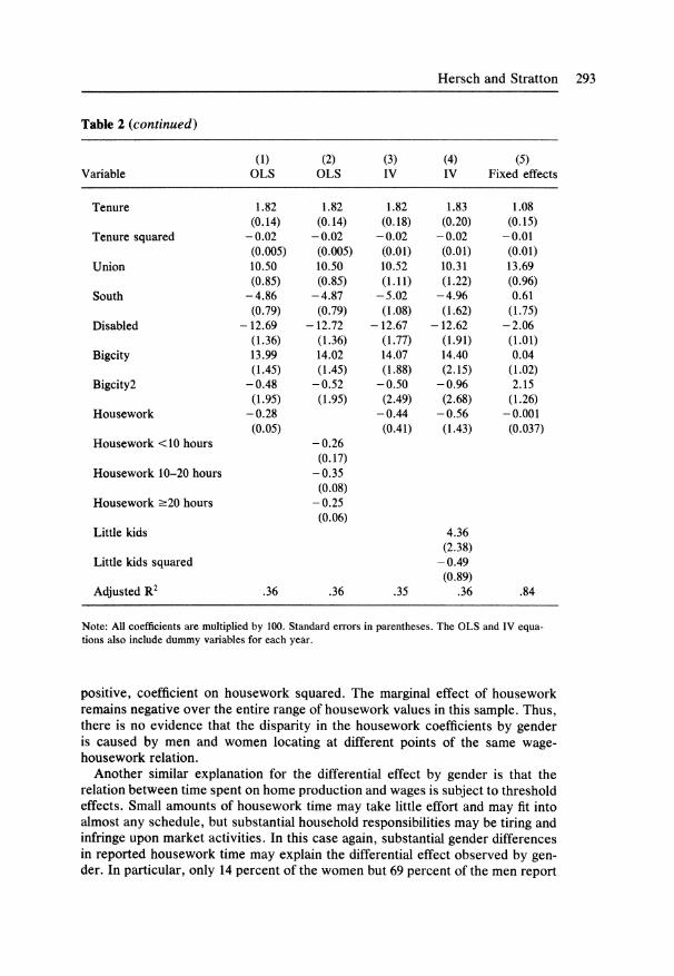
positive, coefficient on housework squared. The marginal effect of housework remains negative over the entire range of housework values in this sample. Thus, there is no evidence that the disparity in the housework coefficients by gender is caused by men and women locating at different points of the same wage- housework relation.

Another similar explanation for the differential effect by gender is that the relation between time spent on home production and wages is subject to threshold effects. Small amounts of housework time may take little effort and may fit into almost any schedule, but substantial household responsibilities may be tiring and infringe upon market activities. In this case again, substantial gender differences in reported housework time may explain the differential effect observed by gender. In particular, only 14 percent of the women but 69 percent of the men report

1.08 (0.15)

-0.01 (0.01) 13.69 (0.96) 0.61

(1.75) -2.06 (1.01) 0.04

(1.02) 2.15

(1.26) -0.001 (0.037)

.84


less than 10 hours of housework time per week. Conversely 8 percent of the men but 50 percent of the women report over 20 hours of housework time per week.

To explore the possibility of threshold effects, we estimate log wage regressions stratifying housework time into three ranges in order to allow the effect of housework to differ with the level of housework. OLS estimates of this modified wage equation are reported in Column 2 of Table 2. These results provide some evidence of a nonlinear relation between housework time and wages, but only for women. Housework time does not significantly affect the wages of women averag- ing fewer than 10 hours of housework a week. Those women spending in excess of 10 hours per week do, however, suffer a wage loss. The estimated impact for those spending 10 to 20 hours on housework is similar to that for those spending over 20 hours, and both of these are similar to that obtained using the continuous housework measure. For men, the coefficients at every level of housework are similar and of the same magnitude as that obtained using the continuous housework measure, although the effect for less than 10 hours is significant at only the 6 percent level. In sum, it would appear that the gender differences in the wage-housework relation are due to women having different slope parameters than men, and not due to women being at a different location on the same nonlinear wage-housework function.11

The evidence of a negative relation for women between housework and wages in cross-sectional analyses is consistent with the findings of other researchers. Of the studies based on OLS estimates, Coverman (1983) finds a significantly negative effect of housework for both husbands and wives using data from the 1977 Quality of Employment Survey. The magnitude of the effect is substantially greater for women, although the difference is not statistically significant. How- ever, Shelton and Firestone (1988) and Hersch (1991b) do not find significant negative effects of housework time on wages for men.12 To investigate whether our results are attributable to differences in either explanatory variables or in functional form, we estimated specifications similar to those estimated in these two studies. Using these alternative specifications, we obtained coefficient estimates on housework similar to those reported in this paper for both the men and women in our samples. This suggests that the divergent results for men are pri- marily due to differences in the measurement of housework and in sample composition.

In particular, Shelton and Firestone (1988) use time diary data for married workers from the 1981 Time Use Study. Their measure of housework includes time spent on both household labor and on child care, and their mean value of housework time for men is nearly twice that found in the PSID sample. The total time spent by men on home production in the sample collected by Hersch (1991b) is also much larger than in the PSID. This may be due to the survey design,

11. Another possible explanation for the gender disparity in the housework effect is that measurement error in reported housework time may be more severe for men than for women. Indeed, a higher noise-to-signal ratio seems likely for men, given their lower level of mean reported housework time. Measurement error will bias the coefficient estimates to zero, but instrumental variables estimation should correct for such bias. 12. Hersch (1991a) uses two-stage least squares to estimate a two-equation wage-housework system,, but also finds a significantly negative effect for women only.


which included a series of prompts for various types of home production, as well as to the timing of data collection (mainly summer, when yard work demands were high). As noted earlier, the effect different housework measures will have on the coefficient of reported housework time is unclear. Furthermore, Hersch (1991b) pools unmarried and married workers, allowing marital status to have only an intercept effect. If the effect of housework on wages differs for men by marital status, the results will not be directly comparable to the results of this paper which include only married workers. Thus, the estimated relation for men appears quite sensitive to the housework measure and to the sample design. Across all studies, however, women consistently incur a greater wage penalty for housework than do men.

B. Instrumental Variables Results

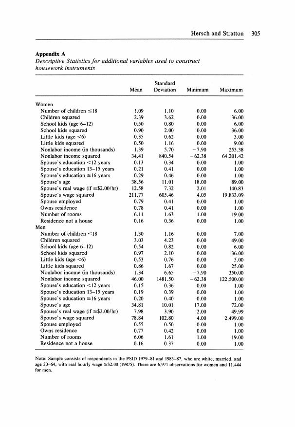
As discussed earlier, housework time may be endogenous. If this is the case, the OLS estimates will be biased and inconsistent. To control for possible simulta- neity bias, we reestimate Equation (1) using instrumental variables. The set of variables available for use as instruments for housework includes nonlabor income,13 spousal characteristics and earnings, information on the number and ages of children in the household, and information on the size, type, and ownership status of the residence. Descriptive statistics for the variables used to construct the housework instruments are presented in Appendix A. Since almost 15 percent of the men's sample reports no time spent on housework, and predictions of housework time for men using OLS regularly generate negative values, the housework instrument for men is constructed using tobit. OLS is used for the women, as fewer than 0.4 percent of the observations indicate no time spent on housework and none of the OLS predicted values are less than zero.

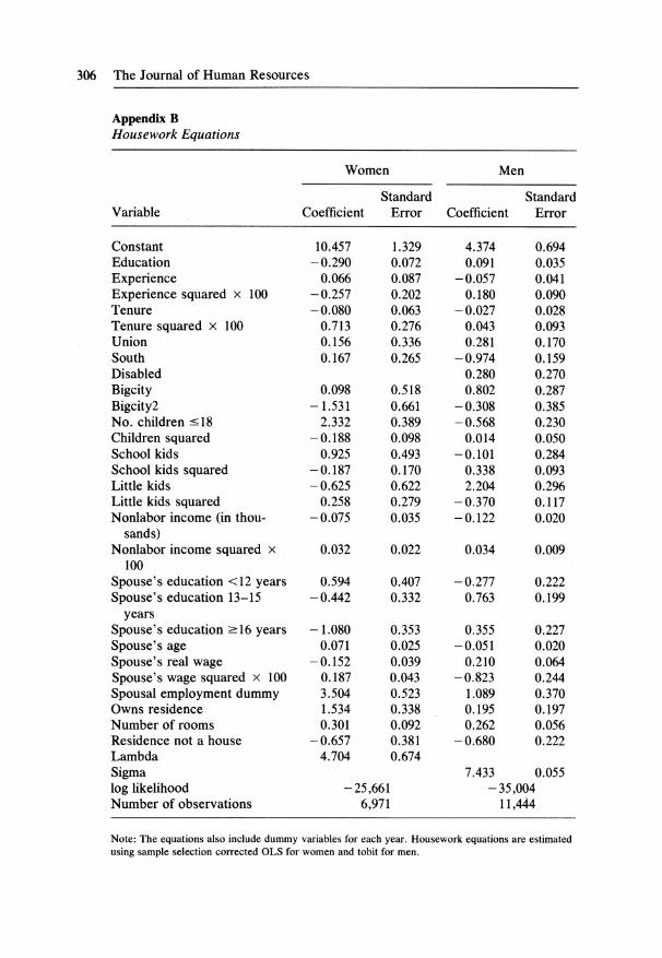
The IV estimates of the wage equation obtained using the complete set of instruments are reported in Column 3 of Table 2.14 The corresponding housework equation estimates are presented in Appendix B. If housework time is endogenous, the coefficient on any variable correlated with housework will be biased. In fact, the coefficient estimates on all variables other than housework are remarkably similar in the OLS and IV estimates. Hausman tests of the hypothesis that housework is exogenous yield test statistics of 5.01 for women and 0.25 for men. These are distributed chi-squared with 19 degrees of freedom. The critical value, assuming a 5 percent significance level, is 30.14. We are unable to reject the hypothesis that housework is exogenous.

An examination of only the housework coefficient is less conclusive, but only for women. The magnitude of the coefficient on housework time increases somewhat for both men and women in the IV specification as compared to the OLS specification, but so does the standard error associated with this coefficient. In-

13. Nonlabor income is the sum of rent, dividends, interest, trust funds, royalties, and (for wives) alimony. 14. Standard errors have been adjusted as necessary for the estimation procedure used. For the women, this entailed correcting the standard errors for the sample selection corrected IV. For the men, the standard errors were corrected for the tobit IV. See Maddala (1983), pp. 243-44.


deed in the men's equation, housework time no longer has a statistically significant effect on wages. Focusing only on the coefficient of housework time, single- parameter Hausman tests of exogeneity yield test statistics of 5.01 for women and 0.16 for men. This is distributed chi-squared with 1 degree of freedom with critical values of 3.84 at the 5 percent level and 6.63 at the 1 percent level. Thus for men, we are unable to reject the hypothesis that housework is exogenous, while for women, we can reject exogeneity at the 5 percent level but not at the 1 percent level.

Given these results, and the well-known problems involving the robustness of IV estimates, we perform a series of sensitivity tests. In particular, we provide tests of the power of the instruments. We also explore the possibilities that some of the instruments are themselves endogenous or that some of the instruments are improperly excluded from the wage equation.

First, we note that a likelihood ratio test of the significance of the instruments not also in the wage equation soundly rejects the hypothesis that these variables have no power for both men and women.15 However, goodness-of-fit measures indicate that the instruments explain a substantial amount of the variation in housework time for women, but explain little for men. R-squared measures of the housework equation rise from 0.087 to 0.154 for women when the instruments not already present in the wage equation are added. Since the men's housework equation is estimated using tobit, the goodness-of-fit measure (McFadden R- squared) is not comparable to the R-squared measure generated by OLS. The comparable OLS estimates of the housework equation for men indicate that the R-squared measures rise from 0.01 to 0.045.

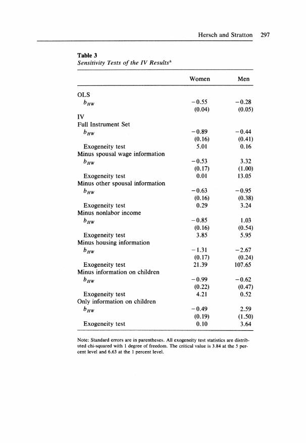
To check the robustness of the IV estimates, we estimated specifications em- ploying several alternative instrument sets, eliminating in turn groups of variables that may possibly be jointly determined with the wage. We note that IV estimation is impossible if there are no exogenous instruments and that any test of the exogeneity of alternative instrument sets requires maintaining the assumption that the common instruments are exogenous. Table 3 summarizes the estimated housework coefficient and, because it is the test that is more likely to reject exogeneity, the single-parameter test statistic for the exogeneity of housework, for a number of alternative specifications.16 The housework coefficients from Table 2, Columns 1 and 3, are repeated for convenience.

As the figures in Table 3 indicate, the results are remarkably stable for women. The effect of housework on wages is similar in magnitude no matter the specifica-

15. The test statistic, distributed chi-squared with 18 degrees of freedom, is 550.5 for the women and 431.6 for the men. 16. We note that endogeneity can be a problem in two ways. First, and of primary interest in this paper, is whether housework is determined endogenously with the wage. The test statistic for the exogeneity of housework entails a comparison of the OLS and IV parameter estimates. The second source arises when the instruments used to model housework are themselves endogenous with the wage. The test statistic (not reported here) for this sort of endogeneity would entail a comparison of the IV estimates obtained using the full instrument set with those obtained using that subset which one holds to be exogenous. The basic notion underlying both tests is that if there is a problem with endogeneity, the parameter estimates will be unstable. For convenience we report test statistics only for the exogeneity of housework.


Table 3 Sensitivity Tests of the IV Resultsa

Women

OLS bHW

IV Full Instrument Set

bHW

Exogeneity test Minus spousal wage information

bHW

Exogeneity test Minus other spousal information

bHW

Exogeneity test Minus nonlabor income

bHW

Exogeneity test Minus housing information

bHw

Exogeneity test Minus information on children

bHW

Exogeneity test Only information on children

bHW

Exogeneity test

-0.55 (0.04)

-0.89 (0.16) 5.01

-0.53 (0.17) 0.01

-0.63 (0.16) 0.29

-0.85 (0.16) 3.85

-1.31 (0.17) 21.39

-0.99 (0.22) 4.21

-0.49 (0.19) 0.10

Men

-0.28 (0.05)

-0.44 (0.41) 0.16

3.32 (1.00) 13.05

-0.95 (0.38) 3.24

1.03 (0.54) 5.95

-2.67 (0.24)

107.65

-0.62 (0.47) 0.52

2.59 (1.50) 3.64

Note: Standard errors are in parentheses. All exogeneity test statistics are distributed chi-squared with 1 degree of freedom. The critical value is 3.84 at the 5 percent level and 6.63 at the 1 percent level.


tion. Of the eight specifications reported, the hypothesis that housework is exogenous can be rejected at the 1 percent level in only one case. In three cases, we can reject exogeneity at the 5 percent level but not at the 1 percent level, and in the remaining four cases, we are unable to reject exogeneity. The findings for men are less robust and indicate that both the magnitude and the sign of the effect are influenced by the choice of instrument set. This is not entirely surprising, given the earlier findings that housework time has no significant impact upon married men's wages in the IV specification and that the full instrument set is only weakly correlated with housework time. That correlation will only be weaker as further instruments are removed.

Finally, we examined the exogeneity of the instrument set by testing the exclusion restrictions imposed on the wage equation. A Lagrange Multiplier test based on the residuals from the IV model with the full instrument set indicates that all of our exclusions are not valid. In Column 4 of Table 2 is an alternative specification of the wage equation which maintained reasonable power for the women's instrument set, did not require substantial modification of the standard log wage specification, and passed the exclusion restriction test.'7 The only instruments for housework used in this analysis were the number of children of various ages. The number of children under age 6 and its square were also added to the wage equation. The remaining four variables included in the instrument list but excluded from the wage equation are significant determinants of housework time for men and women, though the goodness-of-fit of the housework time measure for men is even more suspect.18 As before, the coefficient on housework is negative and significant for women, negative but insignificant for men. In this specification we are unable to reject the null that housework time is exogenous with respect to wages for either men or women.19

Overall, our sensitivity tests give us substantial confidence in our finding of a negative relation between wages and housework for women, but suggest a high degree of uncertainty surrounding the relation for men. Strictly speaking the explanatory power of the instruments is statistically significant for both men and women, but the fit of the housework equation is very poor for men. Consistent with this finding, the estimated housework coefficient for men varies substantially depending on the specification of the instrument set, and while the results generally indicate that there is no significant relation between housework and wages, these results should be taken conditionally. Conversely, the estimates of the housework coefficient for women are remarkably stable with respect to changes in the specification of the instrument set and the wage equation.

17. The Lagrange Multiplier test statistics are 8.00 for women and 8.69 for men. This is distributed chi-squared with 4 degrees of freedom. The critical value at the 5 percent significance level is 9.49. 18. A likelihood ratio test for the significance of these four variables in the housework equation generated a test statistic of 374.48 for women and 35.94 for men. These statistics are distributed chi-squared with 4 degrees of freedom. Hence one can reject the null that these four instruments have no power in the housework equation at the 1 percent significance level. Furthermore, the R-squared measure for the HW equation for women increased from 0.09 to 0.13 by adding these four instruments, indicating that goodness-of-fit is not a problem for the women's sample. 19. The test statistics, distributed chi-squared with 20 degrees of freedom, are 0.43 for women and 0.13 for men.


C. Fixed Effects Results

The IV procedure should control for endogeneity between reported housework time and either component of the error term. However, as reported in Bound, Jaeger, and Baker (1995), while IV estimates are consistent, they are still biased for finite samples and the bias can be substantial even for large samples. Further- more, IV estimates can be inconsistent if the instruments are only slightly correlated with the endogenous variables, as we believe to be the case here for men. An alternative procedure, not subject to these problems, is fixed effects estimation. If the source of the endogeneity is with the individual-specific component of the error term alone, fixed effects estimation provides consistent estimates of the wage-housework effect. Indeed, it seems unlikely that the allocation of household tasks would be renegotiated with every new draw of the random error term Ei, of Equation (1).

Unfortunately, fixed effects estimates also have their drawbacks. Specifically, fixed effects estimates are more sensitive to measurement error than IV estimates-indeed IV estimation typically corrects for measurement error. Fixed effects estimation will correct for persistent individual-specific errors, but can exacerbate measurement error bias when a variable is relatively invariant across time for an individual [see Freeman (1984) for an example]. Thus if the interper- sonal differences in reported housework time are mostly real but the intrapersonal differences are mostly measurement error, fixed effects estimates of the coefficient of housework will be biased to zero. Unfortunately, the downward bias due to measurement error may have a greater effect on the estimates for men because their intrapersonal housework time is particularly invariant across time. Thus, although both IV and fixed effects procedures are used to correct a common problem, they will only yield similar coefficient estimates under ideal circumstances. Under less than ideal circumstances, they provide a useful cross-check of the robustness of the findings.

The coefficient estimates of the fixed effects estimates are presented in Column 5 of Table 2.20 As is usual, this procedure eliminates from the regression any characteristic, observed or unobserved, that is invariant for an individual. Educa- tion is fixed over time for each individual and so drops out of the analysis. Likewise, year dummies and experience measures are nearly perfectly linearly related for men and so year dummies are excluded for men.

Compared with the cross-sectional estimates of Columns 1-4, the fixed effects specification yields smaller returns to both experience and tenure for men, and smaller returns to tenure but larger returns to experience for women. The pre- mium attributed to union coverage increases from 11 to 15 percent for men, but declines from 14 to 7 percent for women. Residence in the South and in a large city are no longer significant. Disability status (for men) is substantially less important. An F-test indicates that the fixed effects are themselves jointly statistically significant.21

20. Fixed effects estimates based on the sample with complete information on the instruments as well as on the variables in the wage equation are essentially identical. 21. The value of the F statistic is 14.6 (df = 1472, 5314) for women and 22.9 (df = 2076, 9387) for men. Since the degrees of freedom are large, the critical value of the F statistic approaches 1.


Of primary interest is the relation between housework time and wages. For both men and women, the estimated housework effect is qualitatively the same in the fixed effects estimates as in the IV estimates. That is, the effect of housework on wages is significantly negative for women, while there is no evidence of a significant effect of housework on wages for men. The magnitude of the effect for women decreases substantially, to about one-third its value in the OLS and IV estimates. Nevertheless, the fixed effects estimates support the conclusion reached earlier that increased time spent on housework does reduce wages for women.

D. Market Hours

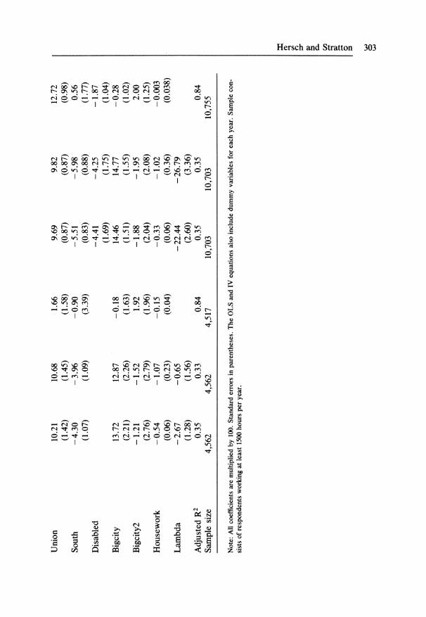
Since conventional theory treats the wage rate as exogenous to the time allocation problem, market hours are generally not included in human capital-based wage formulations (for example, Becker 1965, 1985 and Gronau 1977, 1986). However, fixed employment costs can generate a positive relation between hours of market work and wages (for example, Oi (1962)). We therefore reestimate the counterparts of Columns 1, 3, and 5 of Table 2 for full-time employed workers only (defined as working 1,500 or more hours a year), including the Heckman sample selection correction to control for any bias introduced by this approach. The results are presented in Table 4.22 Restricting the sample to full-time employees makes no difference in the estimated impact of housework on wages in either the OLS or the fixed effects specifications. The IV estimates are of a somewhat larger magnitude and statistically significant for both men and women. Again, however, the instruments explain little of the variation in housework time for men and the men's results are highly sensitive to the choice of instruments. Thus the results are actually qualitatively the same, and despite the possible endogeneity of time spent employed, the effect of housework upon wages does not appear particularly sensitive to market hours.

V. Housework and the Gender Wage Gap

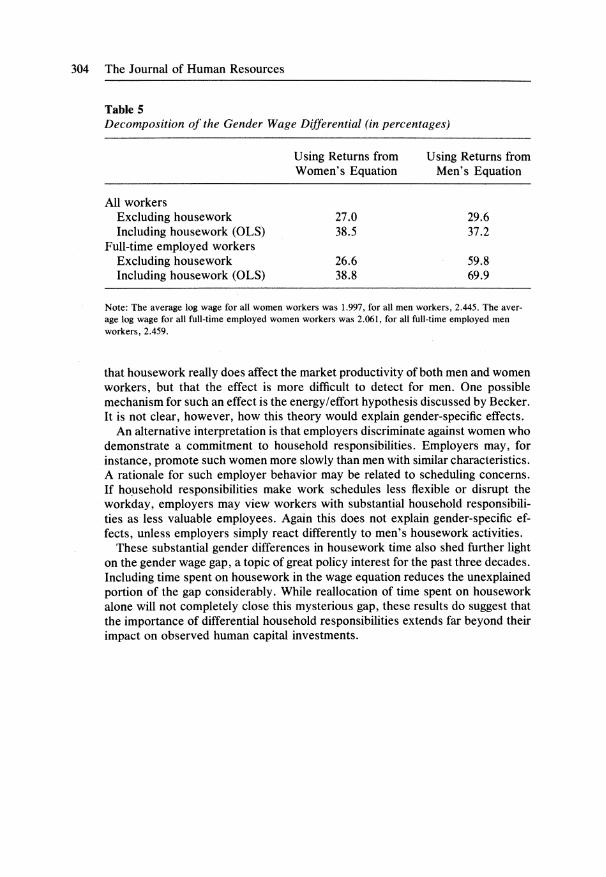
Since married women's housework time is, on average, three times that of married men's, and since pooled cross-section results indicate a substantial negative relation between housework and wages, wage regressions that include housework time should explain a greater share of the gender wage gap. We employ the standard Oaxaca (1973) decomposition to identify that portion of the wage gap which is attributable to differences in observable characteristics and that portion which is attributable to differential returns to those characteristics. This decomposition is conducted by valuing observable characteristics both at the rates estimated for men and at the rates estimated for women. The results are reported in Table 5. In the full-sample specification excluding housework time, differences in observable characteristics explain between 27 and 30 percent

22. The standard errors are corrected for sample selection in Columns 1 and 4, and for sample selection corrected OLS-IV in Columns 2 and 5.


of the gender log wage differential. Controlling for gender differences in time spent on housework increases the explanatory power to about 38 percent, using the OLS estimates.23 The results for the full-time employed sample are similar, with an additional 10-12 percentage points explained by the inclusion of housework time in the wage equations.

The importance of gender differences in housework time to the gender wage gap is considerable and comparable in magnitude to the effect of gender differences in tenure on the gender wage gap. For instance, using the coefficient estimates from the women's wage equation, if women reduced their time on housework to the men's average, their predicted log wage would be 2.06. If instead women increased their tenure to men's average, their predicted log wage would be 2.05.

VI. Conclusions

We examined whether household responsibilities affect wages by estimating wage equations which include time on housework in addition to the customary determinants of wages. The results for women indicate that housework time has a negative effect on wages. This finding is not simply due to a correlation between housework time and unobserved individual characteristics. Instrumental variables results which control for the possible joint endogeneity between housework time and wages yield estimates of a magnitude similar to OLS. Controlling for individual fixed effects reduces, but does not eliminate, the measured impact of housework on wages for women, and the reduction could be due to measurement error bias.

The results for men are less conclusive. The OLS estimates reveal a significant negative effect for men of about half the magnitude as that found for women. We examined and rejected the hypothesis that men and women are at different loca- tions on the same wage-housework function; however, a comparison with the literature suggests that the relation for men is sensitive to the measurement of housework and sample design. Results from the IV and fixed effects specifications indicate that the effect of housework on men's wages is not significant at all. Although the simplest interpretation of these results is that housework time does not affect men's wages, one must keep in mind that both the IV and fixed effects estimates for men may be biased. The instruments, while quite reasonable for women, explain little of the variation in housework time for men. As a result, the IV estimates are imprecise and highly variable. The low intrapersonal variance in housework time undermines the interpretation of the fixed effects estimates by raising the specter of measurement error which would bias the coefficient to housework time toward zero.

In all estimates, we consistently find that the negative effect of housework on wages is substantially as well as statistically significantly greater for women than for men. This finding is subject to multiple interpretations. One interpretation is

23. Using the IV wage equation estimates and controlling for time spent on housework increases the explanatory power of the observable characteristics to 41.5 percent using the men's wage equation, and to 45.6 percent using the women's wage equation.

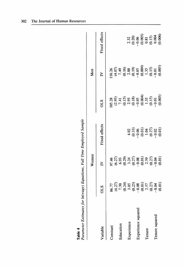
Table 4 Parameter Estimates for In(wage) Equations, Full Time Employed Sample

Women Men

Variable OLS IV Fixed effects OLS IV Fixed effects

Constant

Education

Experience

Experience squared

Tenure

Tenure squared

86.77 (4.27) 7.30

(0.24) 3.05

(0.25) -0.08

(0.01) 2.57

(0.27) -0.04

(0.01)

97.46 (6.27) 6.93

(0.29) 3.24

(0.27) -0.08

(0.01) 2.59

(0.27) -0.04

(0.01)

4.02 (0.33)

-0.06 (0.01) 1.04

(0.27) -0.02 (0.01)

105.28 (2.95) 7.41

(0.15) 2.93

(0.18) -0.05 (0.004) 1.33

(0.15) -0.01 (0.005)

110.26 (4.07) 7.49

(0.16) 2.88

(0.19) -0.05 (0.004) 1.35

(0.15) -0.01 (0.005)

2.32 (0.20)

-0.06 (0.005) 0.81

(0.15) 0.004

(0.006)

0

0-i H 0

'-1 0 C-

0

C) CD

C,)

cp 03

Union 10.21 10.68 1.66 9.69 9.82 12.72 (1.42) (1.45) (1.58) (0.87) (0.87) (0.98)

South -4.30 -3.96 -0.90 -5.51 -5.98 0.56 (1.07) (1.09) (3.39) (0.83) (0.88) (1.77)

Disabled -4.41 -4.25 -1.87 (1.69) (1.75) (1.04)

Bigcity 13.72 12.87 -0.18 14.46 14.77 -0.28 (2.21) (2.26) (1.63) (1.51) (1.55) (1.02)

Bigcity2 -1.21 -1.52 1.92 -1.88 -1.95 2.00 (2.76) (2.79) (1.96) (2.04) (2.08) (1.25)

Housework -0.54 - 1.07 -0.15 -0.33 - 1.02 -0.003 (0.06) (0.23) (0.04) (0.06) (0.36) (0.038)

Lambda -2.67 -0.65 -22.44 -26.79 (1.28) (1.56) (2.60) (3.36)

Adjusted R2 0.35 0.33 0.84 0.35 0.35 0.84 Sample size 4,562 4,562 4,517 10,703 10,703 10,755

Note: All coefficients are multiplied by 100. Standard errors in parentheses. The OLS and IV equations also include dummy variables for each year. Sample consists of respondents working at least 1500 hours per year.

0


Table 5 Decomposition of the Gender Wage Differential (in percentages)

Using Returns from Using Returns from Women's Equation Men's Equation

All workers Excluding housework 27.0 29.6 Including housework (OLS) 38.5 37.2

Full-time employed workers Excluding housework 26.6 59.8 Including housework (OLS) 38.8 69.9

Note: The average log wage for all women workers was 1.997, for all men workers, 2.445. The average log wage for all full-time employed women workers was 2.061, for all full-time employed men workers, 2.459.

that housework really does affect the market productivity of both men and women workers, but that the effect is more difficult to detect for men. One possible mechanism for such an effect is the energy/effort hypothesis discussed by Becker. It is not clear, however, how this theory would explain gender-specific effects.

An alternative interpretation is that employers discriminate against women who demonstrate a commitment to household responsibilities. Employers may, for instance, promote such women more slowly than men with similar characteristics. A rationale for such employer behavior may be related to scheduling concerns. If household responsibilities make work schedules less flexible or disrupt the workday, employers may view workers with substantial household responsibilities as less valuable employees. Again this does not explain gender-specific effects, unless employers simply react differently to men's housework activities.

These substantial gender differences in housework time also shed further light on the gender wage gap, a topic of great policy interest for the past three decades. Including time spent on housework in the wage equation reduces the unexplained portion of the gap considerably. While reallocation of time spent on housework alone will not completely close this mysterious gap, these results do suggest that the importance of differential household responsibilities extends far beyond their impact on observed human capital investments.


Appendix A Descriptive Statistics for additional variables used to construct housework instruments

Standard Mean Deviation Minimum Maximum

Women Number of children <18 1.09 1.10 0.00 6.00 Children squared 2.39 3.62 0.00 36.00 School kids (age 6-12) 0.50 0.80 0.00 6.00 School kids squared 0.90 2.00 0.00 36.00 Little kids (age <6) 0.35 0.62 0.00 3.00 Little kids squared 0.50 1.16 0.00 9.00 Nonlabor income (in thousands) 1.39 5.70 -7.90 253.38 Nonlabor income squared 34.41 840.54 -62.38 64,201.42 Spouse's education <12 years 0.13 0.34 0.00 1.00 Spouse's education 13-15 years 0.21 0.41 0.00 1.00 Spouse's education >16 years 0.29 0.46 0.00 1.00 Spouse's age 38.56 11.01 18.00 89.00 Spouse's real wage (if >$2.00/hr) 12.58 7.32 2.01 140.83 Spouse's wage squared 211.77 605.46 4.05 19,833.09 Spouse employed 0.79 0.41 0.00 1.00 Owns residence 0.78 0.41 0.00 1.00 Number of rooms 6.11 1.63 1.00 19.00 Residence not a house 0.16 0.36 0.00 1.00

Men Number of children <18 1.30 1.16 0.00 7.00 Children squared 3.03 4.23 0.00 49.00 School kids (age 6-12) 0.54 0.82 0.00 6.00 School kids squared 0.97 2.10 0.00 36.00 Little kids (age <6) 0.53 0.76 0.00 5.00 Little kids squared 0.86 1.67 0.00 25.00 Nonlabor income (in thousands) 1.34 6.65 -7.90 350.00 Nonlabor income squared 46.00 1481.50 -62.38 122,500.00 Spouse's education <12 years 0.15 0.36 0.00 1.00 Spouse's education 13-15 years 0.19 0.39 0.00 1.00 Spouse's education >16 years 0.20 0.40 0.00 1.00 Spouse's age 34.81 10.01 17.00 72.00 Spouse's real wage (if >$2.00/hr) 7.98 3.90 2.00 49.99 Spouse's wage squared 78.84 102.80 4.00 2,499.00 Spouse employed 0.55 0.50 0.00 1.00 Owns residence 0.77 0.42 0.00 1.00 Number of rooms 6.06 1.61 1.00 19.00 Residence not a house 0.16 0.37 0.00 1.00

Note: Sample consists of respondents in the PSID 1979-81 and 1983-87, who are white, married, and age 20-64, with real hourly wage >$2.00 (1987$). There are 6,971 observations for women and 11,444 for men.


Appendix B Housework Equations

Women Men

Standard Standard Variable Coefficient Error Coefficient Error

Constant Education Experience Experience squared x 100 Tenure Tenure squared x 100 Union South Disabled Bigcity Bigcity2 No. children -18 Children squared School kids School kids squared Little kids Little kids squared Nonlabor income (in thou-

sands) Nonlabor income squared x

100

10.457 -0.290

0.066 -0.257 -0.080

0.713 0.156 0.167

0.098 -1.531

2.332 -0.188

0.925 -0.187 -0.625

0.258 -0.075

1.329 4.374 0.072 0.091 0.087 -0.057 0.202 0.180 0.063 -0.027 0.276 0.043 0.336 0.281 0.265 -0.974

0.280 0.518 0.802 0.661 -0.308 0.389 -0.568 0.098 0.014 0.493 -0.101 0.170 0.338 0.622 2.204 0.279 -0.370 0.035 -0.122

0.032 0.022

Spouse's education <12 years 0.594 Spouse's education 13-15 -0.442

years Spouse's education >16 years -1.080 Spouse's age 0.071 Spouse's real wage -0.152 Spouse's wage squared x 100 0.187 Spousal employment dummy 3.504 Owns residence 1.534 Number of rooms 0.301 Residence not a house -0.657 Lambda 4.704 Sigma log likelihood Number of observations

0.694 0.035 0.041 0.090 0.028 0.093 0.170 0.159 0.270 0.287 0.385 0.230 0.050 0.284 0.093 0.296 0.117 0.020

0.034 0.009

0.407 -0.277 0.332 0.763

0.353 0.355 0.025 -0.051 0.039 0.210 0.043 -0.823 0.523 1.089 0.338 0.195 0.092 0.262 0.381 -0.680 0.674

-25,661 6,971

0.222 0.199

0.227 0.020 0.064 0.244 0.370 0.197 0.056 0.222

7.433 0.055 - 35,004

11,444

Note: The equations also include dummy variables for each year. Housework equations are estimated using sample selection corrected OLS for women and tobit for men.


References

Becker, Gary S. 1965. "A Theory of the Allocation of Time." Economic Journal 75(299): 493-517.

. 1991. A Treatise on the Family. Cambridge: Harvard University Press. ---. 1985. "Human Capital, Effort, and the Sexual Division of Labor." Journal of

Labor Economics 3 (1, part 2):S33-S58. Blau, Francine D., and Marianne Ferber. 1992. The Economics of Women, Men, and

Work, 2nd ed. Englewood Cliffs, N.J.: Prentice Hall. Bound, John, David A. Jaeger, and Regina M. Baker. 1995. "Problems with Instrumental

Variables Estimation When the Correlation between the Instruments and the Endogenous Explanatory Variable is Weak." Journal of the American Statistical Association 90(430):443-50.

Browning, Martin. 1992. "Children and Household Economic Behavior." Journal of Economic Literature 30(3):1434-75.

Committee on Women's Employment and Related Social Issues and Commission on Behavioral and Social Sciences and Education, National Research Council. 1986. "Explaining Sex Segregation in the Workplace." In Women's Work, Men's Work, ed. Barbara F. Reskin and Heidi I. Hartmann, 37-82. Washington, D.C.: National Academy Press.

Coverman, Shelley. 1983. "Gender, Domestic Labor Time, and Wage Inequality." American Sociological Review 48(5):623-37.

Eisner, Robert. 1988. "Extended Accounts for National Income and Product." Journal of Economic Literature 26(4): 1611-84.

Freeman, Richard. 1984. "Longitudinal Analysis of the Effects of Trade Unions." Journal of Labor Economics 2(1): 1-26.

Fuchs, Victor R. 1988. Women's Quest for Economic Equality. Cambridge: Harvard University Press.

Gronau, Reuben. 1977. "Leisure, Home Production, and Work-The Theory of the Allocation of Time Revisited." Journal of Political Economy 85(6):1099-1123.

- --. 1986. "Home Production-A Survey." In Handbook of Labor Economics, vol. 1, ed. 0. Ashenfelter and R. Layard, 273-304. New York: North-Holland.

Gunderson, Morley. 1989. "Male-Female Wage Differentials and Policy Responses." Journal of Economic Literature 27(1):46-72.

Hersch, Joni. 1991a. "The Impact of Non-Market Work on Market Wages." American Economic Review 81(2):157-60.

. 1991b. "Male-Female Differences in Hourly Wages: The Role of Human Capital, Working Conditions, and Housework." Industrial and Labor Relations Review 44(4): 746-59.

Hill, Martha S. 1985. "Patterns of Time Use." In Time, Goods, and Well Being, ed. F. Thomas Juster and Frank P. Stafford, 133-66. The University of Michigan, Survey Research Center.

Juster, F. Thomas and Frank P. Stafford. 1991. "The Allocation of Time: Empirical Findings, Behavioral Models, and Problems of Measurement." Journal of Economic Literature 29(2):471-522.

Maddala, G. S. 1983. Limited-Dependent and Qualitative Variables in Econometrics. New York: Cambridge University Press.

Oaxaca, Ronald. 1973. "Male-Female Wage Differentials in Urban Labor Markets." International Economic Review 14(3):693-709.

Oi, Walter Y. 1962. "Labor as a Quasi-Fixed Factor." Journal of Political Economy 70(6):538-55.

. 1993. "On Working." Economic Inquiry 31(1):1-28. Shelton, Beth Anne, and Juanita Firestone. 1988. "An Examination of Household Labor

Time as a Factor in Composition and Treatment Effects on the Male-Female Wage Gap." Sociological Focus 21(3):265-78.

housework, fixed effects, and wages of married …stratton...housework, fixed effects, and wages of...

Documents