Household Debt Revaluation and the Real Economy:

Evidence from a Foreign Currency Debt Crisis

Emil Verner†

JOB MARKET PAPER

Gyozo Gyongyosi‡

January 25, 2018

Please click here for most recent version:

http://www.princeton.edu/~verner/JMP.pdf

Abstract

This paper examines how an increase in household debt affects the local economy using a foreigncurrency debt crisis in Hungary as a natural experiment. We construct shocks to local householddebt burdens by exploiting spatial variation in households’ exposure to foreign currency debt duringthe large (over 30%) and unexpected depreciation of the Hungarian forint in late 2008. We firstshow that a shock to local household debt leads to a rise in default rates and a persistent declinein local durable and non-durable consumption. Next, we find that regions with greater exposureto foreign currency debt experience a persistent increase in local unemployment. Firm-level censusdata reveal that employment losses are driven by firms dependent on local demand. Exposed areassee a modest decline in wages, but no adjustment through reallocation toward exporting firmsor migration. In addition to the direct effect of higher debt, we find evidence of local spillovers.Regional exposure to foreign currency debt predicts a decline in house prices and an increase in theprobability of default for households with only domestic currency debt. Our results are consistentwith demand and pecuniary externalities of household foreign currency debt financing.

∗We are extremely grateful to Atif Mian, Mark Aguiar, Adrien Matray, Motohiro Yogo, and Wei Xiong for valuableguidance and encouragement. For helpful comments and discussions at various stages of this project we thankAdrien Auclert, Tamas Briglevic, Markus Brunnermeier, Will Dobbie, Bo Honore, Oleg Itskhoki, Nobukiro Kiyotaki,Graham McKee, Ben Moll, Dmitry Mukhin, Mikkel Plagborg-Møller, Federico Ravenna, Michala Riis-Vestergaard,Eyno Rots, Chris Sims, Amir Sufi, Gianluca Violante, Ben Young, and seminar participants at Princeton University,Danmarks Nationalbank, the National Bank of Hungary, and the 2017 DAEiNA meeting. This research receivedfinancial support from the Alfred P. Sloan Foundation through the NBER Household Finance small grant program.We thank Adam Szeidl for sharing Central European University’s establishment location dataset. Reka Zempleniprovided excellent research assistance. The views in this paper are solely those of the authors and should not beinterpreted as reflecting the views of the National Bank of Hungary.†Princeton University. Contact: (202) 322 8532, verner@princeton.edu, www.emilverner.com.‡Central European University and National Bank of Hungary.

1 Introduction

How does elevated household debt affect the real economy in a crisis? The rapid global increase

in household debt leading up to the Great Recession has revived interest this question. Recent

research, building on Fisher (1933)’s debt-deflation hypothesis, argues that household debt is a

powerful contractionary mechanism because it forces leveraged households to cut back on con-

sumption and leads to fire-sales that depress wealth and borrowing capacity (e.g., Korinek and

Simsek 2016). Since the Great Recession, concerns about the risks of elevated household debt have

led many countries to implement macro-prudential policies that constrain household leverage.1

Despite the prominence of debt-deflation in models and financial regulation, there is limited

empirical evidence that isolates the effects of household debt in a crisis. Several studies find that

expansions in household debt predict more severe recessions (e.g., Jorda, Schularick, and Taylor

2014). However, estimating the causal effect of debt on real outcomes presents several empirical

challenges. First, increases in household debt are often part of a broader cycle in real activity and

credit conditions, making it difficult to disentangle whether debt itself causes more severe recessions.

For example, in the years surrounding the Great Recession, household leverage is strongly correlated

with the rise and subsequent collapse in house prices and credit availability, both across countries

and across U.S. regions.2 Second, testing the equilibrium effects of debt requires variation in

household debt at a sufficiently aggregated level. For example, higher debt may raise individual

labor supply, but this expansionary effect may be offset by declines in local demand and house

prices.

In this paper, we provide causal evidence on the real economic effects of a sudden increase

in household debt burdens using a foreign currency debt crisis in Hungary as a natural experi-

ment. We exploit spatial variation in exposure to household foreign currency debt during the sharp

depreciation of the Hungarian forint in the 2008 global financial crisis. Using this household debt

1Macro-prudential restrictions such as caps on loan-to-value or debt-to-income ratios were in place in over 41 countriesin 2014, including China, South Korea, and the United Kingdom (Cerutti, Claessens, and Laeven 2017).

2Country-level data show that credit expansions predict house price declines, bank credit contractions, equity marketcrashes, distressed corporate balance sheets, and over-optimistic expectations (Schularick and Taylor 2012, Jorda,Schularick, and Taylor 2013, Baron and Xiong 2017, Krishnamurthy and Muir 2017, Lopez-Salido, Stein, andZakrajsek 2017, Mian, Sufi, and Verner 2017, IMF 2017). Dynan (2012) analyzes whether household debt overhangconstrained consumption in the U.S. during the Great Recession, but notes that debt is strongly correlated withregional housing booms and busts, which Mian and Sufi (2014a) show have strong effects on local consumption andemployment.

1

revaluation shock, we provide three main results. First, household debt revaluation increases house-

hold default rates and persistently depresses consumption. Second, the increase in household debt

causes a significantly worse local recession. The worse recession is driven by a decline in demand

through two channels: a direct effect of debt on demand and an indirect effect through a decline in

house prices. Third, as a result, we find that the debt revaluation has negative spillovers on nearby

households without foreign currency debt.

Household exposure to foreign currency debt in a currency crisis provides a novel way to assess

the real economic effects of higher debt. Hungary provides an appealing setting for this analysis for

two reasons. First, prior to the depreciation of the Hungarian forint in late 2008, 69% of household

debt was denominated in foreign currency. Second, the depreciation of the forint was sharp and

unexpected. The flight to safety from emerging markets in late 2008 caused the forint to depreciate

by over 30%, raising aggregate household debt by 10% of disposable income. While we focus

on Hungary, foreign currency retail lending, especially to households, was widespread throughout

emerging Europe during the 2000s. It resulted in an unprecedented level of private sector currency

mismatch, with non-financial foreign currency debt reaching 19% of GDP in 2007 for a sample of

10 new EU member states (Ranciere, Tornell, and Vamvakidis 2010).3

Hungary’s foreign currency debt revaluation allows us to address the identification challenge

that household debt usually varies as part of a broader credit and real economic cycle. We show

that local exposure to household foreign currency debt is not correlated with household leverage

in 2008 or growth in house prices, durable spending, and real activity prior to the currency crisis.

Our empirical strategy, therefore, estimates the effect of higher household debt, holding fixed other

related factors such as a house price boom and bust (e.g., Mian and Sufi 2011), over-optimistic be-

liefs about future growth or returns (e.g., Bordalo, Gennaioli, and Shleifer 2017, Kaplan, Mitman,

and Violante 2017), or a housing supply overhang (e.g., Gao, Sockin, and Xiong 2017, Rognlie,

Shleifer, and Simsek 2017). A distinct concern in our setting is that the exchange rate depreciation

differentially affects local outcomes through channels other than household debt, such as expendi-

ture switching or corporate foreign currency debt. However, the currency composition of household

debt is not strongly related to local export intensity, industry composition, or corporate foreign

3This statistic is based on data from national central banks collected by Brown, Peter, and Wehrmuller (2009).Household foreign currency denominated debt was also important in previous emerging market crises. For example,prior to Argentina’s crisis and devaluation in 2002, 80% of mortgages were denominated in U.S. dollars (IMF 2003).

2

currency financing. Instead, variation in household foreign currency exposure is mainly driven by

the historical banking market structure and the initial depth of domestic banks.

To analyze the consequences of the household debt revaluation, we use administrative house-

hold credit registry data from Hungary to construct a new dataset on household debt and default

at the individual and regional level. We match these household credit data at the regional level

with: (i) measures of household spending, unemployment, and house prices, and (ii) firm-level cen-

sus and credit registry data that include information on employment, bank lending relationships,

and balance-sheet items, including the currency composition of firms’ liabilities. Our data, there-

fore, provide a complete picture of private foreign currency financing, allowing us to compare the

consequences of household versus firm foreign currency debt in a currency crisis.

We first show that household debt revaluation leads to a strong increase in household defaults

and a decline in consumption. Using data across 3,124 local areas (cities or municipalities), we find

that a 1% increase in debt leads to a 0.17 percentage point increase in default rates, a 2.7% decline

in auto expenditure, a proxy for durable spending, and a 0.22% decline in electricity usage, a proxy

for non-durable consumption. The strong consumption response to debt revaluation implies that

households are not hedged against their foreign currency debt positions, opening up the possibility

for demand externalities on local employment.

Next, we investigate how household debt revaluation affects local employment. Standard models

have differing implications for the effect of debt revaluation on real activity. In an open economy

model with household currency mismatch and nominal rigidity, debt revaluation triggers a decline

in consumption and employment. The fall in employment is larger in economies with greater

home bias. By contrast, in a model with flexible prices, debt revaluation lowers consumption, but

increases employment, as households boost labor supply.

In the data, we find that regions with greater exposure to foreign currency debt experience

a significant decline in local employment and a persistent rise in unemployment. The rise in

unemployment is consistent with the importance of local household demand effects and is larger

in more urban areas, where we expect less “leakage” of local demand to other regions. Exploiting

firm-level census data, we show that the decline in employment is driven by non-exporting firms

and firms in the non-tradable sector. These firms also experience significant drops in sales and

output. By contrast, exporting firms are unaffected. In terms of magnitudes, we estimate that a

3

10 percentage point increase in household debt-to-income raises the local unemployment rate by

0.8 to 1.6 percentage points.

Why does household debt revaluation lead to persistently higher local unemployment? One

potential reason is a lack of labor market adjustment through wage declines, migration, or reallo-

cation to exporting firms. Indeed, we find that, concurrent with the decline in employment, areas

with greater exposure to foreign currency debt see only a modest decline in wages and no increase

in migration or reallocation toward exporting firms.

Another potential mechanism that amplifies the effects of higher debt burdens is house price

declines, which reduce household wealth and borrowing capacity. We find that, despite experiencing

similar house price growth before the depreciation, regions with more exposure to foreign currency

debt experience a significant relative decline in house prices after the depreciation. House price

declines, in turn, predict lower household consumption. The amplification through house price

declines is broadly consistent with recent models of pecuniary externalities from collateralized

foreign currency borrowing (e.g., Mendoza 2010, Bianchi 2011, Korinek 2011). Liquidity constraints

also amplify households’ response to debt revaluation. Borrowers with foreign currency debt are

more likely to default if their debt is of shorter maturity, holding fixed total debt.

The finding that debt revaluation causes a rise in unemployment and decline in house prices is

consistent with theories where debt has negative demand and fire-sale externalities (e.g., Farhi and

Werning 2016). An implication of these theories is that borrowing in foreign currency has negative

spillover effects on other households in the crisis, including households that did not borrow in

foreign currency. We find direct evidence of such spillovers in loan-level data. In particular, we find

that borrowers who live in regions with greater exposure to foreign currency debt are more likely

to default, conditional on borrowers’ own foreign currency debt position. The effect of regional

foreign currency exposure on the probability of default holds even for borrowers with only domestic

currency debt.

The final part of the paper analyzes the connection between household foreign currency debt and

a traditional channel of emerging market crises: corporate foreign currency indebtedness (Krugman

1999, Aghion, Bacchetta, and Banerjee 2000). Using firm-level data, we find that firms with

foreign currency debt cut investment sharply after the depreciation, relative to unexposed firms.

Surprisingly, however, these firms see stronger sales growth and similar employment growth. This

4

is explained by the fact that firms borrowing in foreign currency tend to be larger, more productive,

and more likely to be exporters (see also Salomao and Varela 2016). As a result, local employment

declines in the crisis can be more easily explained by households’ foreign currency debt than firms’

foreign currency debt, although there is evidence of an interaction between the two channels.

We take several steps to support our identifying assumption, namely that the debt revaluation

shock is not correlated with unobserved shocks affecting local economic outcomes. The estimates

are statistically and economically similar when controlling for initial household income, leverage,

demographics, export exposure, and industry composition. In firm-level data, our results are robust

to controlling for relationship-specific bank lending shocks (e.g., Chodorow-Reich 2014), industry-

specific shocks, and firm characteristics including size, leverage, productivity, and ownership struc-

ture. Moreover, trends in all outcome variables are similar in the years leading up to the forint

depreciation in the fall of 2008. Further, we find null effects using the 1998 Russian Sovereign

Debt Crisis, which spilled over to other emerging markets, as a placebo sample. Our results are

not explained by higher historical cyclicality in more exposed regions. Finally, we show that the

estimates are similar when instrumenting for household foreign currency debt exposure using an

instrument that exploits spatial variation in bank market shares and their propensity to lend in

foreign or domestic currency. This allays the concern that foreign currency exposure is driven by

currency-specific credit-demand factors that are correlated with business cycle risk.

Related Literature. This paper connects with literatures in finance, macroeconomics, and inter-

national finance. It contributes to a growing literature on household leverage and business cycles.

Recent models emphasize that a combination of high household debt, deleveraging, and house price

declines can trigger a recession in the presence of macroeconomic frictions, such as sticky prices,

real rigidities, and monetary policy constraints (Hall 2011, Eggertsson and Krugman 2012, Guerri-

eri and Lorenzoni 2015, Midrigan and Philippon 2016, Huo and Rıos-Rull 2016). Mian, Rao, and

Sufi (2013) and Baker (2016) show that leverage amplifies the consumption response to income and

wealth shocks. By contrast, we trace the effect of a shock directly to household debt and study the

impacts on local firms, house prices, and real allocations.

Our analysis is connected to recent papers that use variation in borrower payments from interest

rate changes. Recent studies find that borrowers who experience interest rate reductions, through

5

interest rate resets or refinancing, have a lower probability of default and use additional funds to

increase spending on durables (Tracy and Wright 2012, Fuster and Willen 2013, Di Maggio et al.

2017, Agarwal et al. 2015). In the framework of Auclert (2016), these papers study the interest

rate exposure channel, whereas we estimate the Fisher channel through a revaluation of liabilities.4

In addition, we focus mainly on local equilibrium effects, given the large foreign currency debt

revaluation in Hungary, and show that foreign currency financing has negative spillover effects.

Existing studies primarily focus on borrower-level responses.5

Another related line of papers evaluates the effects of debt reduction policies. Agarwal et al.

(2016) find that U.S. regions exposed to mortgage modifications through HAMP saw fewer foreclo-

sures, smaller house price declines, and a modest increase in durable spending.6 Consistent with

the theoretical analysis of Eberly and Krishnamurthy (2014), Ganong and Noel (2016) show that

only reductions in current payments impact default and consumption at the individual level. In

contrast to these studies that focus on debt reduction for heavily indebted borrowers, we focus on

unanticipated increases in debt burdens for a broad population of debtors, starting from “normal”

conditions. Therefore, we also contribute to the debate on mortgage contract design (Shiller and

Weiss 1999, Mian and Sufi 2014a, Guren, Krishnamurthy, and McQuade 2017). Our findings show

that low-interest foreign currency contracts, which tend to impose losses on borrowers in bad times

(Lustig and Verdelhan 2007, Brunnermeier, Nagel, and Pedersen 2008), have adverse real economic

effects and spillovers on other individuals.

Finally, this paper contributes to the international finance literatures on currency crises and

adjustment to international wealth transfers. A large literature on balance-sheet effects in currency

crises has focused on firm and bank foreign currency indebtedness.7 To our knowledge, our paper

is the first to analyze the effects of household foreign currency exposure, despite the prevalence of

4In Auclert (2016) the Fisher channel arises due to revaluation of nominal debt from inflation, whereas we examinerevaluation of foreign currency debts from a depreciation.

5Di Maggio et al. (2017) and Agarwal et al. (2015) present evidence that higher zip code exposure to interest ratedeclines boosted local spending, employment, and house prices.

6Dobbie and Goldsmith-Pinkham (2015) present evidence that protection from unsecured creditors raised regionalconsumption and employment in the Great Recession.

7Eichengreen and Hausman (2005) provide an overview of foreign currency financing in emerging markets. A num-ber of studies analyze the causes and consequences of firm foreign currency exposures in emerging market crises(Caballero and Krishnamurthy 2003, Aguiar 2005, Gilchrist and Sim 2007, Kim, Tesar, and Zhang 2015, Du andSchreger 2015, Kalemli-Ozcan, Kamil, and Villegas-Sanchez 2016). Cross-country studies find that the country-levelFC debt exposure increases the probability and severity of a sudden stop crisis (e.g., Calvo, Izquierdo, and Mejia2008), but the use of aggregate data makes it difficult to disentangle the role of household, firm, and bank balancesheet effects, as well as other country-level shocks and policy responses.

6

household foreign currency debt throughout emerging Europe in the 2000s and in previous emerg-

ing market crises. In addition, whereas the extant empirical literature has documented a foreign

currency balance-sheet effect at the firm level, we show that foreign currency exposure has local

aggregate effects. More generally, our estimates isolate the effects of an outward transfer on wages

and real allocations. Our paper, therefore, brings empirical evidence to the classic Transfer Prob-

lem debate (Keynes 1929, Ohlin 1929).

Outline. The remainder of the paper is structured as follows. Section 2 discusses the background

of the foreign currency debt crisis in Hungary. Section 3 discusses the theoretical framework and

empirical methodology. Section 4 describes the data. Sections 5 through 8 present the results, and

Section 9 concludes.

2 The Hungarian Foreign Currency Debt Crisis

Hungary experienced a large expansion in household credit between 2000 and 2008. Figure 1(a)

shows that over this period household debt to GDP increased by 28 percentage points.8 The expan-

sion was financed by two categories of loans: government-subsidized local currency (LC) housing

loans and unsubsidized foreign currency (FC) loans.9 In September 2008, 69% of outstanding hous-

ing debt was denominated in foreign currency, primarily Swiss franc, directly exposing household

balance sheets to the large depreciation of the Hungarian forint starting in October 2008.

Household lending was initially spurred by a government housing program that provided interest

rate subsidies on long-term LC mortgages. The subsidy program was introduced in 2000 to grant

households access to housing finance at rates that were more affordable than the high market

interest rates of over 10%. The subsidies fixed nominal interest rates for borrowers at levels similar

to euro interest rates (4-6%), with the government financing the 5-6.5 percentage point spread

relative to the market interest rate for domestic currency loans.10

8As a comparison, U.S. household debt increased by a similar amount relative to GDP, albeit from a much higherinitial level of 66% in 2000.

9Unsubsidized local currency loans with market interest rates comprised less than 10% of local currency housing loansin September 2008.

10The typical subsidized mortgage loan had a 15- to 20-year maturity with a fixed rate for the first five years andcapped interest rates paid by households at 6%. This placed all interest rate risk on the government budget. Thesubsidy scheme also provided a 40% personal income tax deduction on mortgage repayments. Vas and Kiss (2003)and Kiss and Vadas (2005) describe housing finance policies in Hungary.

7

Subsidized lending growth was driven primarily by three major domestic mortgage banks. The

market for housing loans was highly concentrated, since average retail banking density following

the transition from socialism was low and domestic mortgage banks had a tax advantage in orig-

inating subsidized loans (Rozsavolgyi and Kovacs 2005). Therefore, domestic subsidized housing

credit growth was strongest in regions with a higher historical density of domestic mortgage banks.

However, the subsidies placed a significant burden on public finances and subsidies on new loans

were sharply curtailed in early 2004.

The increased cost of LC loans for borrowers led foreign banks to enter the retail lending market

and compete with domestic banks by offering low-interest-rate FC housing loans. Foreign banks

competing for market share expanded FC credit aggressively, especially to areas with a lower density

of domestic subsidized credit, both by opening new branches and through mortgage agents (Banai,

Kiraly, and Nagy 2011). Foreign currency retail lending was prevalent throughout Europe prior

to the 2008 financial crisis, especially in new EU member states.11 Interest rates on Swiss franc

and euro loans averaged 4% to 6%, which implied savings of about 5 percentage points relative to

domestic currency loans at market rates, holding the exchange rate constant. Figure 1(b) shows

an acceleration in FC credit growth in the middle of 2004.

The foreign currency credit expansion was propelled by a stable exchange rate. Figure 2(a)

shows that the euro-forint exchange rate remained stable up to October 2008, as the National

Bank of Hungary (MNB) maintained a crawling band with respect to the euro. Meanwhile, the

Swiss franc was quasi-fixed against the euro, so the Swiss franc-forint exchange rate mirrored

the euro exchange rate prior to the crisis.12 Further, Hungary ascended to the EU in May 2004

and initially targeted adopting the euro in 2007. Survey evidence shows that the expectation of

adopting the euro boosted FC loan demand (Fidrmuc, Hake, and Stix 2013). Moreover, in a survey

from November 2008, Pellenyi and Bilek (2009) find that 87% of respondents with an FC loan did

11Lending to households in foreign currencies was widespread during the 2000s in Estonia, Latvia, Lithuania, Croatia,Serbia, Bulgaria, Poland, Romania, and Ukraine (Yesin 2013). Swiss franc mortgage lending was prevalent inAustria starting in the mid-1990s. Swiss franc and yen lending also occurred in Denmark, Spain, and the UK,especially prior to the 2008 financial crisis.

12Between January 1, 1999 and June 4, 2003, Hungary maintained a pre-announced ±2.25% crawling band aroundthe euro. The band widened to ±15% in June 2003, but, in practice, fluctuations remained within ±5% (Ilzetzki,Reinhart, and Rogoff 2010). The forint primarily hovered at the strong end of the band up until 2008. Ilzetzki,Reinhart, and Rogoff (2010) classify the Swiss franc as fluctuating within a de facto ±2% moving band against theeuro, and the Swiss franc-euro (or D-mark) volatility was low for several decades up to the Eurozone crisis (Beer,Ongena, and Peter 2010).

8

not expect exchange rate volatility at the late 2008 level. The mid-2008 Consensus Forecast also

predicted that the forint-euro exchange rate would remain constant.

The depreciation of the forint in October 2008 was not caused by distress in household credit

markets. This makes the Hungarian currency crisis a promising natural experiment to study the

consequences of household debt revaluation. The National Bank of Hungary abandoned the crawling

band in February 2008, and in October 2008, the flight to safety away from emerging markets led

to a sharp depreciation of emerging market currencies, including the forint. The depreciation of

the forint was particularly strong because of investor concerns about the Hungarian government’s

large external financing needs.13 Between September 2008 and March 2009, the forint depreciated

by 27.5% against the euro and 32.3% against the Swiss franc. The forint weakened further against

the Swiss franc in 2010 and 2011, as the Swiss franc appreciated during the Eurozone crisis.

Figure 2(b) shows that this depreciation raised the value housing debt in terms of domestic

currency by 5-9% of disposable household income in 2009 (2.5-4.5% of 2008 GDP), and 10% of

disposable income by 2010 (5% of GDP), relative to a counterfactual where exchange rates had

remained at their September 2008 values. Regional variation in the debt-revaluation shock depicted

in Figure 2(b) is the fundamental shock we exploit in our empirical analysis.14

The depreciation was associated with a current account reversal and a severe recession. Figure

3 panel (a) shows that the current account reversed from a deficit of 8% of GDP to a small surplus.

Real output contracted by 7.4% relative to its peak in 2008Q2 and remained depressed for several

years, before beginning a moderate recovery in 2013. Private consumption fell more than output

and had yet to recover to its pre-crisis level by early 2015. Durable expenditure, in particular, saw a

complete collapse, falling an astonishing 36.7% from 2008 to 2010, a figure comparable to the decline

in the U.S. Great Depression (Figure 3(c)).15 The enormous decline in consumer spending stands

out relative to other sudden stop episodes and provides suggestive evidence for the importance of

household debt revaluation in this setting.16

13Hungary negotiated a $25 billion loan from the IMF and EU to meet the government’s external financing gap inlate October 2008.

14Starting in 2011, the newly elected conservative government implemented a variety of policies to alleviate the sharprise in monthly installments. These efforts culminated in the conversion of the entire stock of foreign currency loansinto domestic currency in late 2014. Our analysis focuses on the period between 2008 and 2011, prior to when thesepolicies were implemented.

15Durable spending in the U.S. fell 32.4% in the Great Depression according to Romer (1990).16Mendoza (2010) shows that, in a sample of 33 emerging market sudden stop episodes, aggregate consumption

typically falls slightly less than output.

9

3 Theory and Empirical Framework

3.1 Theory

The debt-deflation channel is generally an endogenous transmission channel that amplifies shocks

to the economy (King 1994). Our approach in order to isolate the debt-deflation channel is to

obtain direct variation in real debt burdens using a foreign currency debt revaluation as a natural

experiment. In this section, we outline the mechanisms through which a household debt revaluation

can affect economic activity. We highlight that the debt revaluation shock provides a clean way to

separate several classes of models.

Consistent with the foreign currency debt crisis in Hungary, we assume that domestic households

can borrow and save in domestic and foreign currency risk-free debt. In the initial steady state,

the nominal exchange rate equals one, and the household has D∗ > 0 foreign currency debt, where

debt is measured relative to steady state income.17

At time zero, there is an unanticipated, one-time exchange rate depreciation from one to 1+∆e >

1. Because of currency mismatch on household balance sheets, total debt after the depreciation

increases by ∆eD∗. The domestic output response at time t ≥ 0 to the exchange rate shock in the

presence of household foreign currency debt can be written as:

yt = βt∆eD∗︸ ︷︷ ︸

Debtrevaluation

+ γt∆e.︸ ︷︷ ︸Expenditure

switching

(1)

In appendix C we formally show that this equation can be derived from a New-Keynesian small

open economy model in which we assume households have foreign currency debt exposure in the

initial steady state. The model follows the framework of Galı and Monacelli (2005) and Farhi and

Werning (2017) and provides expressions for βt and γt as a function of the underlying parameters.

The exchange rate shock affects the economy through two channels. The first channel on the

right-hand-side of (1) is the household debt revaluation channel. The debt-revaluation, in turn, can

affect the economy through various mechanisms. One mechanism in expansionary. An increase in

household debt lowers households’ wealth and consumption, which leads households to boost labor

17Households in Hungary had substantial foreign currency debt but essentially no deposit “dollarization.”

10

supply, raising output.18

At the same time, the increase in the households’ real debt burden will depress consumption

and therefore demand. The decline in demand for home goods is larger when the degree of home

bias, households’ propensity to consume home goods relative to foreign goods, is larger. Home

bias is partly due to the presence of non-tradable goods, and below, we explicitly test whether the

decline in demand has a stronger effect on firms producing non-tradable goods.

As a result of the opposing expansionary supply and contractionary demand effects, the sign

of βt in the short-run can be positive or negative. With flexible prices, the labor supply effect

dominates, and an increase in debt boosts output in the short run, as in the model of Devereux and

Smith (2007). In this case, β is (weakly) positive in the short run.19 In contrast, in the presence

of nominal rigidities, the rise in real debt burdens depresses output through a demand effect, and

β is negative in the short run. Estimation of βt, therefore, provides a clean test of flexible versus

sticky price models.

An important implication of nominal rigidities is that the contractionary effect of a debt-induced

decline in demand is not internalized by individuals when making financing decisions. This implies

that there is a demand externality of borrowing decisions (Farhi and Werning 2016, Korinek and

Simsek 2016). This is especially true for riskier forms of borrowing that impose greater losses

in bad times, such as foreign currency borrowing in funding currencies, as households undervalue

insurance against adverse shocks. By utilizing loan-level data, we will explicitly test for whether

FC financing has negative impacts on other households, including households that did not borrow

in FC.

In addition to nominal rigidities, the rise in debt may further depress consumption and thus

output in the presence of financial constraints, such as a collateral constraint on housing debt. The

rise in debt may increase defaults and foreclosures, leading to fire sales that depress local house

prices. A decline in house prices amplifies the initial wealth loss for all households and can tighten

collateral constraints, further lowering consumption (Kiyotaki and Moore 1997, Iacoviello 2005).

18The labor supply expansion channel holds for most standard preferences assumed in the literature. An exceptionis GHH (quasi-linear) preferences, which eliminate the wealth effect on labor supply.

19Similarly, Chari, Kehoe, and McGrattan (2005) and Lorenzoni (2014) show that a sudden stop can boost output byinducing households to expand labor supply. However, debt can also lower labor supply through a debt overhangeffect (e.g. Dobbie and Song 2015, Donaldson, Piacentino, and Thakor 2016). Given that there was no consumerbankruptcy code in Hungary at the time of the crisis and therefore a small degree of limited liability, the wealtheffect likely dominates the debt overhang effect in this context.

11

A worse recession also depresses house prices, creating a two-way feedback between the demand

and fire-sale channels. We explore this channel empirically below. Further, if households have

a precautionary savings motive, the increase in debt would induce households to further reduce

consumption to maintain a sufficient buffer of savings. Finally, real rigidities, such as frictions that

inhibit a reallocation of employment towards exporting firms, strengthen the negative effects of

debt on output (Huo and Rıos-Rull 2016).

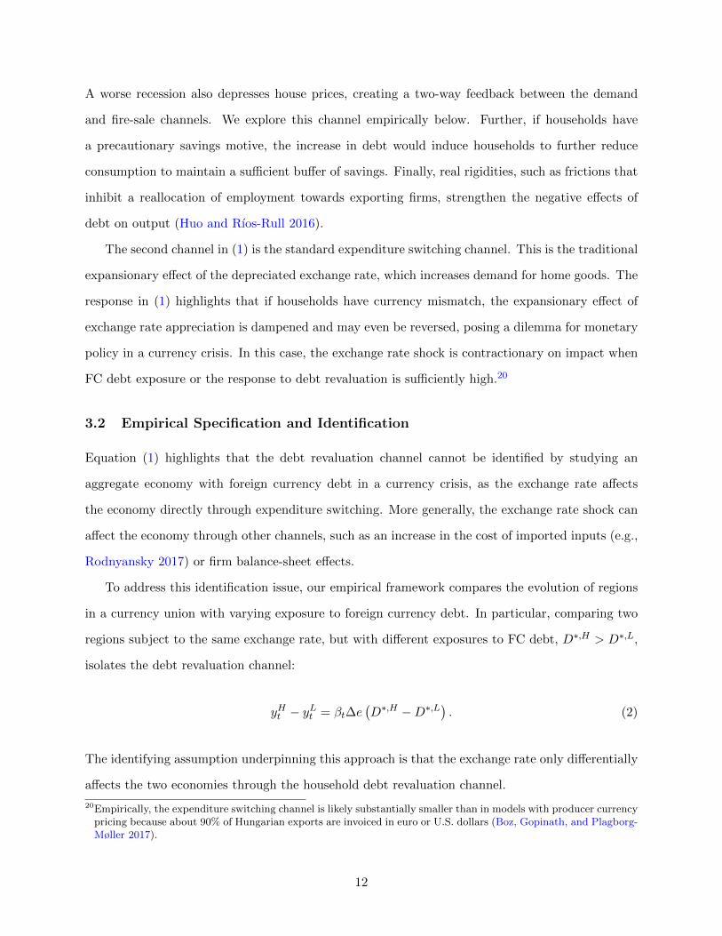
The second channel in (1) is the standard expenditure switching channel. This is the traditional

expansionary effect of the depreciated exchange rate, which increases demand for home goods. The

response in (1) highlights that if households have currency mismatch, the expansionary effect of

exchange rate appreciation is dampened and may even be reversed, posing a dilemma for monetary

policy in a currency crisis. In this case, the exchange rate shock is contractionary on impact when

FC debt exposure or the response to debt revaluation is sufficiently high.20

3.2 Empirical Specification and Identification

Equation (1) highlights that the debt revaluation channel cannot be identified by studying an

aggregate economy with foreign currency debt in a currency crisis, as the exchange rate affects

the economy directly through expenditure switching. More generally, the exchange rate shock can

affect the economy through other channels, such as an increase in the cost of imported inputs (e.g.,

Rodnyansky 2017) or firm balance-sheet effects.

To address this identification issue, our empirical framework compares the evolution of regions

in a currency union with varying exposure to foreign currency debt. In particular, comparing two

regions subject to the same exchange rate, but with different exposures to FC debt, D∗,H > D∗,L,

isolates the debt revaluation channel:

yHt − yLt = βt∆e(D∗,H −D∗,L

). (2)

The identifying assumption underpinning this approach is that the exchange rate only differentially

affects the two economies through the household debt revaluation channel.

20Empirically, the expenditure switching channel is likely substantially smaller than in models with producer currencypricing because about 90% of Hungarian exports are invoiced in euro or U.S. dollars (Boz, Gopinath, and Plagborg-Møller 2017).

12

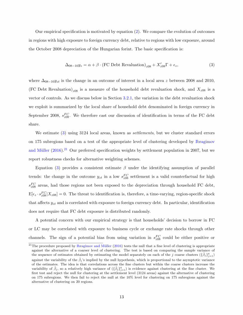
Our empirical specification is motivated by equation (2). We compare the evolution of outcomes

in regions with high exposure to foreign currency debt, relative to regions with low exposure, around

the October 2008 depreciation of the Hungarian forint. The basic specification is:

∆08−10yz = α+ β · (FC Debt Revaluation)z08 +X ′z08Γ + εz, (3)

where ∆08−10yzt is the change in an outcome of interest in a local area z between 2008 and 2010,

(FC Debt Revaluation)z08 is a measure of the household debt revaluation shock, and Xz08 is a

vector of controls. As we discuss below in Section 3.2.1, the variation in the debt revaluation shock

we exploit is summarized by the local share of household debt denominated in foreign currency in

September 2008, sFCz08. We therefore cast our discussion of identification in terms of the FC debt

share.

We estimate (3) using 3124 local areas, known as settlements, but we cluster standard errors

on 175 subregions based on a test of the appropriate level of clustering developed by Ibragimov

and Muller (2016).21 Our preferred specification weights by settlement population in 2007, but we

report robustness checks for alternative weighting schemes.

Equation (3) provides a consistent estimate β under the identifying assumption of parallel

trends: the change in the outcome yzt in a low sFCz08 settlement is a valid counterfactual for high

sFCz08 areas, had those regions not been exposed to the depreciation through household FC debt,

E[εz · sFCz08|Xz08] = 0. The threat to identification is, therefore, a time-varying, region-specific shock

that affects yzt and is correlated with exposure to foreign currency debt. In particular, identification

does not require that FC debt exposure is distributed randomly.

A potential concern with our empirical strategy is that households’ decision to borrow in FC

or LC may be correlated with exposure to business cycle or exchange rate shocks through other

channels. The sign of a potential bias from using variation in sFCz08 could be either positive or

21The procedure proposed by Ibragimov and Muller (2016) tests the null that a fine level of clustering is appropriateagainst the alternative of a coarser level of clustering. The test is based on comparing the sample variance ofthe sequence of estimates obtained by estimating the model separately on each of the j coarse clusters ({βj}qj=1)

against the variability of the βj ’s implied by the null hypothesis, which is proportional to the asymptotic varianceof the estimates. The idea is that correlations across the fine clusters but within the coarse clusters increase thevariability of βj , so a relatively high variance of ({βj}qj=1) is evidence against clustering at the fine cluster. Wefirst test and reject the null for clustering at the settlement level (3124 areas) against the alternative of clusteringon 175 subregions. We then fail to reject the null at the 10% level for clustering on 175 subregions against thealternative of clustering on 20 regions.

13

negative. Regions with a higher FC share could be more export-intensive, high-income areas with

less exposure to business cycle risk, or areas where households receive a higher fraction of income in

foreign currency, biasing our estimates toward zero. For example, Beer, Ongena, and Peter (2010)

find that Swiss franc borrowers in Austria are typically high-income and financially sophisticated

households. On the other hand, sFCz08 may be correlated with exposure to negative business cycle

shocks. For example, less financially sophisticated households that are more exposed to recession

risk may select into FC loans because they do not adequately assess exchange rate risk.

An important supply-side determinant of the cross-regional variation in foreign currency debt

share is the initial depth of domestic retail banks. Following the transition from communism,

average retail banking depth and competition were low relative to other countries in the region,

but varied substantially across regions.22 Areas with a higher density of domestic banks experi-

enced stronger growth in subsidized domestic currency household credit. Following the removal

of domestic currency subsidies in 2004, foreign banks filled in to areas with lower branch density,

offering foreign currency loans with significantly lower interest rates than market rates on domestic

currency debt. Appendix Table A.1 confirms that areas with a lower banking density in 1995 have

a higher domestic currency debt-to-income in 2008, lower FC debt-to-income, and therefore a lower

share of debt in FC.

Extant research on the determinants of FC borrowing in Hungary using household surveys finds

that FC and LC borrowers are broadly similar along observable dimensions such as demographic

characteristics and risk tolerance, although FC borrowers on average have slightly lower income

than LC borrowers (Fidrmuc, Hake, and Stix 2013, Pellenyi and Bilek 2009). To get a sense of

the balancedness of sFCz08 across observables at the settlement level, Table 2 presents regressions of

sFCz08 on various settlement-level characteristics.23 Goldsmith-Pinkham, Sorkin, and Swift (2017)

show that identification in Bartik-style instruments comes from exogeneity of the shares, so the

correlation between the FC debt share and observables gives an indication of the potential for

biased estimates.

Table 2 shows that the FC debt share is uncorrelated with export exposure, consistent with the

22Gal (2005) provides a detailed analysis of the geographic differences in the density of retail banking after thetransition from socialism, showing that there are significant differences in the number of retail banks per capitaacross regions. He argues these differences are driven by a high degree of centralization in a few major cities datingback to socialism.

23Figure A.1 visually presents binned bivariate means for the key tests in Table 2.

14

assumption that allows us to isolate the debt revaluation channel of the exchange rate shock. FC

debt exposure is also balanced across debt to income, manufacturing and construction employment

shares, growth in disposable income over 2004-08, the working age population share, labor pro-

ductivity, and corporate FC indebtedness. Below, we also find that sFCz08 is uncorrelated with the

change in other outcomes, including house prices and durable spending prior to the depreciation.

This allows us to disentangle the impact of higher debt from other housing-related factors that may

contribute to a more severe recession. Consistent with the survey evidence, high sFCz08 areas do tend

to have lower disposable income per capita and lower population.

In the empirical exercises below, we report estimates for specifications that control for these

settlement-level observables to capture any time-varying shocks that interact with these observables.

In particular, we control for the 2008 debt to disposable income, log 2008 population, log 2008

disposable income per capita, the share age 18-59, the share age 60 or above, industry employment

shares, export revenues as a share of total firm revenues, and export revenues relative to total

firm revenues. We also control for the intensity of a public jobs program that was expanded in

2011.24 In firm-level employment regressions, we include firm-level measures of productivity, size,

firm leverage and firm FC indebtedness, ownership structure, two-digit industry fixed effects, and

fixed effects for firm-bank relationships prior to the depreciation.

We take a number of additional steps to provide support for the parallel trends assumption.

First, we present tests that control for time-varying regional shocks by including fixed effects for

20 regions. We also present robustness to controlling for 175 subregion-specific time trends. This

ensures that the estimates are not driven by subregion-specific secular trends or shocks that may

be spuriously correlated with FC debt exposure at a more aggregated regional level.

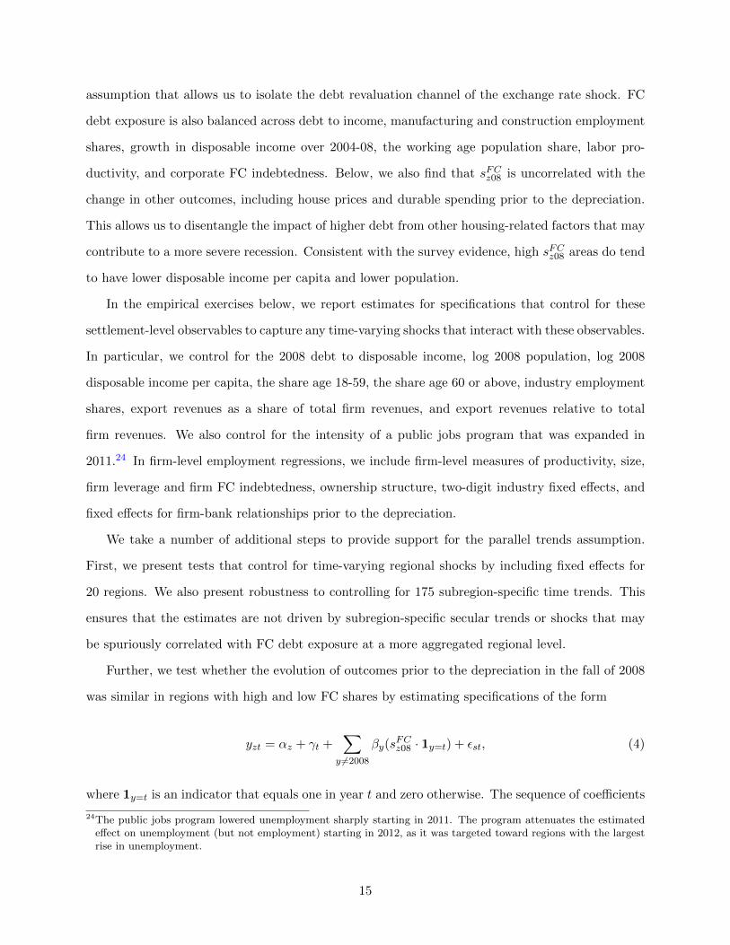
Further, we test whether the evolution of outcomes prior to the depreciation in the fall of 2008

was similar in regions with high and low FC shares by estimating specifications of the form

yzt = αz + γt +∑

y 6=2008

βy(sFCz08 · 1y=t) + εst, (4)

where 1y=t is an indicator that equals one in year t and zero otherwise. The sequence of coefficients

24The public jobs program lowered unemployment sharply starting in 2011. The program attenuates the estimatedeffect on unemployment (but not employment) starting in 2012, as it was targeted toward regions with the largestrise in unemployment.

15

{βy} shows the evolution of yzt from 2008 in high FC share regions relative to low FC share regions.

The finding that βy is insignificant and close to zero in years leading up to the depreciation supports

the parallel trends assumption. We also conduct placebo tests using the 1998 Russian Sovereign

Debt Crisis that spilled over to emerging markets. Finally, to control for currency-specific credit

demand factors, we present robustness tests using an instrument for sFCz08 that exploits a bank’s

propensity to lend in foreign or domestic currency times the bank’s presence in a given region.

3.2.1 Measuring Household Balance-Sheet Exposure to the Depreciation

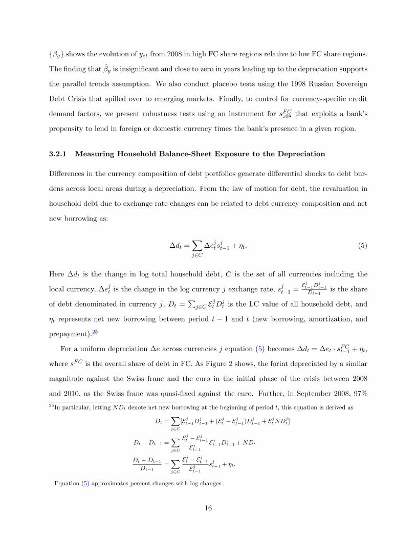
Differences in the currency composition of debt portfolios generate differential shocks to debt bur-

dens across local areas during a depreciation. From the law of motion for debt, the revaluation in

household debt due to exchange rate changes can be related to debt currency composition and net

new borrowing as:

∆dt =∑j∈C

∆ejtsjt−1 + ηt. (5)

Here ∆dt is the change in log total household debt, C is the set of all currencies including the

local currency, ∆ejt is the change in the log currency j exchange rate, sjt−1 =Ejt−1D

jt−1

Dt−1is the share

of debt denominated in currency j, Dt =∑

j∈C EjtD

jt is the LC value of all household debt, and

ηt represents net new borrowing between period t − 1 and t (new borrowing, amortization, and

prepayment).25

For a uniform depreciation ∆e across currencies j equation (5) becomes ∆dt = ∆et · sFCt−1 + ηt,

where sFC is the overall share of debt in FC. As Figure 2 shows, the forint depreciated by a similar

magnitude against the Swiss franc and the euro in the initial phase of the crisis between 2008

and 2010, as the Swiss franc was quasi-fixed against the euro. Further, in September 2008, 97%

25In particular, letting NDt denote net new borrowing at the beginning of period t, this equation is derived as

Dt =∑j∈C

[Ejt−1Djt−1 + (Ejt − E

jt−1)Dj

t−1 + EjtNDjt ]

Dt −Dt−1 =∑j∈C

Ejt − Ejt−1

Ejt−1

Ejt−1Djt−1 +NDt

Dt −Dt−1

Dt−1=∑j∈C

Ejt − Ejt−1

Ejt−1

sjt−1 + ηt.

Equation (5) approximates percent changes with log changes.

16

of FC debt was denominated in Swiss franc. A settlement’s share of debt in FC as of 2008:9,

sFCz08, captures most of the variation in exposure to the depreciation, so we use sFCz08 as the baseline

measure of exposure to the depreciation. We measure exposure as of September 2008, the last

month before the depreciation, but results are very similar using earlier months in the summer of

2008 or instrumenting the 2008 FC debt share with the share in 2005 or 2006.

To obtain estimates that are more easily interpretable, we directly estimate the effect of the

household debt revaluation shock from 2008:9 to t, ∆dz,08−t, using:

∆dz,08−t =

∑j∈C

(Ejt+hD

jz08 − E

j08D

jz08

)Dz08

, (6)

The debt revaluation shock can be related to the FC shares as: ∆dz,08−t =∑

j∈C [(Ejt+h−Ej08)/Ej08]sjz08.

Thus, ∆dz,08−t captures the valuation effect on household debt as the weighted average exchange

rate depreciation applied to debt, with the currency shares as the weights.

We also present robustness tests using the household debt revaluation relative to income, which

is defined as

∆dIncz,08−t =

∑j∈C

(Ejt+hD

jz08 − E

j08D

jz08

)(Household disp. income)z08

. (7)

Holding fixed the currency composition of debt, higher leverage yields a higher debt revaluation to

income shock. The two measures of debt revaluation are positively correlated, with a correlation

coefficient of 0.26. Finally, we also assess robustness using the fraction of loans on FC, the number

of FC loans per adult, and the share of mortgage debt in FC (i.e. excluding home equity loans).

4 Data and Summary Statistics

We construct a dataset at the region level with information on household debt by currency and

loan type, default, spending, unemployment rate, house prices, wages, and demographic variables.

The primary level of aggregation in our data is a settlement (a city or municipality). There are

3,152 settlements in Hungary with an average population of 3,168 in 2010. We also present results

for 175 subregions that approximate local labor markets (Paloczi et al. 2016). We match this

17

regional dataset with firm-level data on employment and balance-sheet information, including firm

FC liabilities and banking relationships. This section summarizes the key features of the data.

Appendix B provides further details on the data sources and variable definitions.

4.1 Household Credit Registry

We use loan-level data from the Hungarian Household Credit Registry to measure household debt

balances, new borrowing, and default at the loan and settlement level. The household credit

registry contains all loans extended by all credit institutions to private individuals outstanding on

or after March 2012. The credit registry records information on the loan type, loan amount, date

of origination, maturity, monthly payments, default status, and currency.26 The household credit

registry also reports the identity of the lender and the borrower’s settlement of residence.

In order to measure a settlement’s FC debt exposure prior to the late 2008 forint depreciation,

we reconstitute the credit registry going back to 2000. Specifically, we use an annuity model to

estimate monthly payments and outstanding debt prior to 2012 for the population of outstanding

loans at the start of the credit registry. The reconstructed credit registry accounts for 80.5% of

aggregate housing debt in the Financial Accounts in September 2008. Moreover, the default rate

for loans in the credit registry closely matches the aggregate default rate reported separately from

bank balance sheets prior to and during the crisis. The annuity model also performs well at the

loan level. For example, a cross-sectional loan-level regression of the actual balance on the modeled

balance in 2012 yields an R2 of 83%. We describe the annuity model in detail and further evaluate

its accuracy in Appendix B.

Loans that are terminated (repaid, refinanced, canceled) before 2012 but were outstanding in

September 2008 present a potential measurement error problem for the estimation of a settlement’s

FC debt exposure. In the fall of 2011, the newly elected Hungarian government implemented an

Early Repayment Program that allowed borrowers with a foreign currency mortgage or home equity

loan to repay the loan in full at a preferential exchange rate of 20-30% below the prevailing market

rates. The program retired 21% of outstanding foreign currency debt.27 Accounting for the 2011

26Default status is effectively available starting in 2008. The household credit registry was preceded by a negativeregistry that contained information on delinquency.

27It is widely believed that the program benefited wealthier and more creditworthy borrowers, since the programrequired full repayment of the loan and provided a limited 60 day window to participate.

18

Early Repayment Program raises the coverage of the credit registry in 2008:9 from 80.5% to 96%

of housing debt in the flow of funds.

In Appendix B we use two approaches to adjust our outstanding settlement-level debt measures

for loans that are prepaid through the Early Repayment Program. The first adjustment uses a

separate dataset on the universe of loans for three of the largest banks in Hungary that have a

combined market share of 24%. We use information from these three banks to approximate the

amount of debt repaid through the 2011 ERP in each settlement for all other banks. The second

approach imputes the amount of debt prepaid in a settlement with the amount of new domestic

currency borrowing (refinancing) during the window when the Early Repayment Program was in

operation. Appendix B shows that all the main results in this paper are quantitatively similar when

controlling for the 2011 Early Repayment Program using these adjustments. Furthermore, in our

main analysis, we control for covariates that may potentially be associated with participation in

the 2011 Early Repayment Program, including disposable income and demographic characteristics.

4.2 Settlement and Firm-Level Data

The main settlement-level variables are from the Hungarian Central Statistics Office (KSH). We

proxy for settlement household durable spending using new auto registrations.28 To proxy for non-

durable consumption, we use the quantity of electricity consumed by households. KSH also provides

settlement-level information on household income, tax payments, population, and net migration.

Local unemployment rate data are based on the number of registered job seekers relative to

working-age population from the National Employment Service (NFSZ). We estimate settlement-

level nominal hourly wages from the Structure of Earnings Survey, an annual survey of about 150-

200 thousand workers, adjusting for compositional changes in the workforce following the procedure

outlined in Beraja, Hurst, and Ospina (2016). We also use annual settlement and subregional house

price indexes estimated from the National Bank of Hungary’s home purchase transactions database.

Firm-level data are from corporate tax filings to the Hungarian Tax Authority (NAV) and

include employment, payrolls, total sales, export sales, and value-added growth at the firm level for

all double-bookkeeping firms in Hungary. The median firm has one establishment (including the

28Auto registrations have been used as a proxy for durable spending in several recent papers including Mian and Sufi(2012) and Agarwal et al. (2016).

19

headquarters), and, on average, a firm has establishments in 1.66 settlements. We therefore define

a firm’s exposure to household FC debt by the settlement of the headquarters.29 We clean the

sample of firms following previous research on NAV data (e.g., Endresz and Harasztosi 2014). In

particular, we exclude firms with fewer than 3 employees and firms in the finance, real estate, public

administration, education, and health and social work sectors. This yields a sample of 80,447 firms

in 2008 that we follow through the crisis. Finally, we compute firm FC debt exposure by matching

loan-level data from the Hungarian Firm Credit Registry.

4.3 Summary Statistics and Variation in Household Foreign Currency Exposure

Panels A and B of Table 1 report summary statistics for the 3124 settlements (cities or munici-

palities) in our sample. The foreign currency debt share in September 2008, sFCz08, has a mean of

66% and a standard deviation of 8.7 percentage points. Figure 4(a) presents a map of the spatial

variation in the household FC debt share, revealing that the share of household debt in foreign

currency is not strongly clustered in specific regions.

Figure 4(b) provides a visual impression of the variation in FC debt exposure by computing

the average sFCz08 within 20 equal population bins. The lowest exposure bin has an FC debt share

of 40%, while settlements in the highest bin have an average FC share of almost 90%. Foreign

currency exposure generates an average debt revaluation shock, ∆08−10dz, of 22%. The majority

of household FC debt is denominated in Swiss franc, with an average across settlements of 97% in

2008:9.

Table 1 panel B shows that the household default rate rose by 4.1 percentage points on average,

while the unemployment rate increased by 2.1 percentage points. The data also show a staggering

70% (120 log point) decline in auto spending over the same period, a 2% fall in electricity con-

sumption, and a 15% decline in house prices. The mean level of settlement debt to disposable

income is 50%. Panel C reports summary statistics for our sample of firms. Average employment

growth from 2008 to 2010 was -12.9%. The average firm size is 34 employees, a quarter of firms are

exporters, and 21% are in the manufacturing sector.

29The establishment address dataset was created by researchers at Central European University with funding providedfrom the European Union framework NETWORKS-283484. The original data were made available by WoltersKluwer Kft. Results are similar if we only use single-establishment firms or if we take the establishment weightedaverage of household FC debt exposure.

20

5 Household Responses to Debt Revaluation

5.1 Household Balance Sheets and Default

We begin by documenting that settlements with more exposure to household FC debt experience

significant financial distress following the depreciation of the Hungarian forint. Table 3 presents

regressions of various measures of changes in household debt on the household FC debt share, sFCz08.

Columns 1 and 2 show that the FC debt share is strongly correlated with the household debt

revaluation shock measured between 2008:9 and 2010:9, ∆08−10dz. The estimate implies that a

settlement with full exposure to FC debt experiences a 26% revaluation in household debt, relative

to a settlement with an FC debt share of zero. The R2 of this regression is 0.95, which shows that

the FC debt share captures most of the variation in the debt revaluation shock, as we discussed in

Section 3.2.1.

In columns 3 through 5 we replace the debt revaluation shock with growth in overall household

debt as the dependent variable. Columns 3 and 4 show that from 2008:9 to 2010:9, a settlement

with an FC debt share of one experiences a 26 to 33% increase in debt relative to a settlement

with only local currency debt. The similarity between the estimates in columns 1-2 and 3-4 implies

regions with more exposure to foreign currency debt do not deleverage to a greater extent following

the depreciation. Column 5 shows that the estimate increases to about 40% by 2011. Columns 6

and 7 replace the growth in debt with the change in debt relative to 2008 household disposable

income. Consistent with an initial debt to income ratio of about 50% in 2008, foreign currency

debt exposure raises debt to 2008 income by about half the percentage increase in debt.

Table 4 analyzes the effect of debt revaluation on the household default rate. Housing loans in

Hungary are full recourse loans, and debt cannot be discharged in bankruptcy. Thus, a household’s

decision to default reflects limited ability, as opposed to willingness, to repay. Column 1 shows

a regression of the change in the fraction of housing loans in arrears between 2008 and 2010 on

household FC debt exposure. The estimate implies that taking the FC debt share from zero to one

is associated 7.2 percentage point higher settlement housing default rate. The coefficient is large in

magnitude. A one standard deviation increase in sFCz08 implies a one-quarter of a standard deviation

increase in the household default rate.

In columns 2-4 we add various controls that may affect the estimation. In particular, in columns

21

2 and 3 we progressively add controls for demographic characteristics, debt to income, log disposable

income, export exposure, 18 one-digit industry employment shares, and fixed effects for 7 main

regions (NUTS 2). The estimate falls by one-fifth, but remains significant at the 1% level. As we

discuss in detail below, applying the test from Oster (2016) and Altonji, Elder, and Taber (2005)

for coefficient stability, we can reject that the effect is driven by omitted variable bias.

Finally, columns 5 and 6 present the estimated effect in terms of the household debt revaluation

shock, ∆08−10dz. This specification can be thought of as the “second stage” regression of the effect

of debt revaluation on default, where the second stage variable is computed as the exact debt

revaluation shock implied by FC debt exposure.30 In terms of magnitudes, column 6 implies that

a 10% increase in household debt raises the settlement default rate by 1.7 percentage points. In

Section 7.3 we unpack this result using loan-level specifications. We find that more exposed areas

experience a rise in defaults because (i) they have a greater share of FC loans, which have a higher

default rate than LC loans, and (ii) loans in exposed regions are more likely to default, which

indicates a role for negative local equilibrium effects.

Figure 5 presents the effect of FC debt exposure on the default rate over time. It plots the

estimates of {βy} from estimating equation (4) for the settlement default rate on housing loans at a

quarterly frequency. The omitted period is 2008Q1, the first period default information is available

in the credit registry. The evolution of the default rate in high and low FC debt regions is similar

up to the depreciation. Higher FC debt regions only begin experiencing high default rates starting

in 2008Q4. The default rate rises differentially in more exposed settlements through 2014.

5.2 Durable Spending and Non-Durable Consumption

In Figure 3 we saw that real aggregate private consumption fell by over 10% from 2008 to 2010,

and durable spending declined by 40%. Micro data on the number of auto registrations point to

a 60% decline in new auto registrations in 2009 alone. In Table 5 we ask whether this dramatic

decline in spending is related to the household debt revaluation across local areas.

Table 5A columns 1-4 report regressions of the change in log new auto registrations from 2008

to 2010 on the household FC debt exposure, sFCz08.31 Between 2008 and 2010, settlements with only

30As can be inferred from Table 3, results are almost identical if we instead instrument the increase in householddebt with the FC debt share.

31To allow for small settlements with zero registrations, we add one before taking logs, i.e. ln(1+Czt). The estimates

22

FC debt see a 63% (99.5 log point) decline in auto spending relative to regions with no foreign

currency debt. A one standard deviation increase in sFCz08 is associated with one-fifth of a standard

deviation lower auto expenditure. The estimated effect is robust to including baseline controls for

demographic characteristics, income, and household debt to income, as well as controls for export

exposure, industrial composition, and fixed effects for seven major regions. In columns 5 and 6

we replace the FC debt share with the household debt revaluation shock and find that a 1% debt

revaluation lowers household durable spending by 2.7 to 3.5%.

Figure 6 panel (a) illustrates how FC debt exposure affects new auto registrations over time by

plotting estimates of {βy} from equation (4). In the years leading up to the depreciation there is

no differential change in auto spending in high relative to low sFCz08 settlements. In particular, there

is no evidence of differential “boom-bust” dynamics. The estimated effect on durable spending

after the depreciation is therefore unlikely to be explained by a combination of: (i) a consumption

boom reversal, (ii) an overhang of consumer durables in more exposed regions, and (iii) a reversal

in optimistic growth expectations. In 2009, following the depreciation, auto spending falls sharply

in regions with a higher FC share and continues to fall in 2010. Durable spending begins a slow

recovery starting in 2012, but remains significantly below the pre-crisis level even by 2014. The per-

sistent effect on durable expenditure is consistent with the fact that debt revaluation permanently

lowers household wealth.

Table 5 panel B examines the effect of FC debt exposure on household electricity consumption,

a proxy for non-durable consumption. Even for this subset of consumption that we expect to be

relatively inelastic, we find a negative and significant estimate. The estimate on sFCz08 ranges from

-13.1% without controls to -7.3% with our full set of controls. The implied elasticity with respect

to the household debt revaluation shock in columns 5-6 ranges between −0.22% and −.47%.

Figure 6(b) shows the dynamic impact of FC debt exposure on non-durable consumption. Again,

we can reject the notion that high FC debt exposure regions have differential consumption growth

up to 2008. After the depreciation, non-durable spending falls from 2008 to 2009 and 2010. As

with durable expenditure, the debt revaluation shock appears to permanently lower household

consumption in more exposed regions.

are quantitatively similar when dropping small settlements with zero spending in either period or when using thesymmetric growth rate, C10z−Cz08

.5(C10z+Cz08), which allows for the start or end value to be zero.

23

6 Impact of Debt Revaluation on Real Activity

6.1 Main Result

The rise in the real burden of debt for households with foreign currency exposure leads to a rise in

default rates and a sharp decline in household spending. But how does the local economy absorb

this shock? The evidence on default and consumption alone does not inform us about whether

the debt revaluation shock had a negative impact on local economic activity. Households may

respond to the rise in debt burdens by boosting search effort or hours in order to service higher

debt payments. However, a positive effect on labor supply may be overwhelmed by a shortfall

in local demand, especially in the presence of price and wage rigidities and reallocation frictions,

leading to a decline in employment and a rise in unemployment.

Table 6 explores the effect of household debt revaluation on the settlement (city or municipality)

unemployment rate. Column 1 reveals that settlements with higher exposure to household FC debt

see a larger rise in unemployment from 2008 to 2010. The coefficient implies that a region with all

debt denominated in FC experiences a 2.3 percentage point increase in unemployment from 2008 to

2010, relative to a region with only domestic currency debt. Columns 2 through 4 reveal that the

estimate is unchanged when including various controls, including household income and leverage,

export exposure controls, one-digit industry employment shares, and region fixed effects.

In terms of economic magnitudes, Table 6 columns 5 and 6 show that a 10% revaluation of

household debt raises local unemployment by 0.7-0.9 percentage point. This result implies that a

higher burden of debt leads to a significantly weaker local economy. The weaker local economy, in

turn, exacerbates the burden of debt repayment.

Figure 7 presents the full dynamic impact of FC debt exposure on unemployment from estimat-

ing equation (4). Between 2003 and 2008, there is a precisely estimated zero relationship between

sFCz08 and the change in unemployment, consistent with parallel trends. Notably, parallel trends hold

during 2005 and 2006, when the aggregate unemployment rate increased by 1.5 percentage points

following the implementation of a fiscal consolidation program (Figure 3). After the depreciation

in 2008Q4, the coefficient rises to 2.2 percentage points, and unemployment remains persistently

higher in more exposed regions for several years. By 2014, six years after the shock, unemployment

in exposed regions had still not completely recovered to its relative pre-crisis level.

24

6.2 Local Demand: Outcomes at Tradable and Non-tradable Firms

The differential decline in consumption and rise in unemployment in regions that are more exposed

to FC debt is evidence that household debt revaluation affects the local economy through a decline

in household demand. Debt revaluation should therefore more strongly affect firms catering to local

markets (Mian and Sufi 2014b). To provide further evidence for a local household demand channel,

we draw on firm-level census data to test whether the debt-revaluation shock leads to a stronger

decline in employment, sales, and output for non-exporting firms and firms in the non-tradable

sector.

Table 7 panel A displays estimates of the effect of household FC debt exposure on firm-level

employment growth:

gEi,08−10 = βsFCz08 +Xi08Γfirm +Xz08Γsettlement + αindustry + εib,

Following the employment dynamics literature (Davis and Haltiwanger 1999), we measure firm-

level employment growth as the symmetric growth rate in employment between 2008 and 2010,

gEi08−10 = 100(Ei10−Ei08).5(Ei10+Ei08) .

32

In Table 7 column 1, we find that firms in settlements with greater exposure to the household

debt revaluation shock experience a significant decline in employment.33 Estimating the equation at

the firm level allows us to control for detailed firm characteristics. Column 2 shows that the elasticity

is stronger when including firm-level controls, our baseline settlement level controls, and two-digit

NACE industry fixed effects. Firm-level controls are a firm’s own FC debt share, a quadratic in

2008 log employment, 2008 log sales, leverage (debt-to-sales ratio) in 2008, and indicator variables

for whether the firm is majority state or foreign owned. Two-digit industry fixed effects ensure that

the estimate is not driven by industry-specific employment shocks that are correlated with regional

variation in sFCz08.

32The symmetric growth rate is equivalent to the log difference up to a second order Taylor approximation, but isbounded between -200 and 200, which mitigates the influence of outliers.

33Table A.2 panel B shows the estimates are robust to using the debt revaluation relative to income as the right-hand-side variable. Table A.3 shows that results are similar when controlling for firm-level lagged employment growth,ensuring that the estimates are not driven by trends in firm employment. Table A.4 presents the same regressionfor firm-level data aggregated to the settlement level and finds similar results. Further, Figure A.2 present thesettlement level employment estimates over time, showing that the employment decline is persistent and is notdriven by pre-trends.

25

Table 7 columns 3-6 estimate the effect separately for non-exporters and exporters. The decline

in employment is driven entirely by non-exporting firms. Relative to a settlement with no FC debt,

non-exporting firms in a settlement with all debt in FC experience a 16% greater decline in employ-

ment, relative to a settlement where all debt is in LC. In contrast, employment at exporting firms

is shielded from the variation in local demand induced by the debt revaluation. This test provides

additional evidence that the household debt revaluation effect on employment is not spuriously

driven by the exchange rate channel or another shock to exporters.

In columns 7 and 8 we focus on firms in the non-tradable sector, following Mian and Sufi (2014b).

Specifically, we classify the restaurant and retail industries and four-digit NACE industries with

below-median geographic Herfindahl indexes as non-tradable.34 We also exclude firms that have

positive exports in 2008, since these are less likely to cater primarily to local markets. Focusing on

the subset of firms in the non-tradable sector yields an estimate on household FC debt exposure of

-13.3% with controls, which is similar to the overall decline for non-exporters.

Table 7 panels B and C present the same regressions for domestic sales growth and output (real

value-added) growth.35 Household FC debt exposure predicts a decline in domestic sales and real

value added, and the magnitudes are similar to the effect on employment. The effect on household

FC debt exposure is larger among non-exporters and firms in the non-tradable sector, while sFCz08 is

not significantly correlated with sales growth or real output growth for exporters.

6.3 Interpretation

The decline in local employment and the rise in unemployment from the household debt revaluation

is qualitatively consistent with the presence of price rigidities. To provide a sense of the potential

aggregate effects of the debt revaluation channel, one can compute an aggregate partial equilibrium

counterfactual in which all settlements have zero foreign currency liabilities. To do this, we sort

settlements into 20 equal population bins and apply the estimated coefficient from Table 6 to the

average foreign currency share in each bin and aggregate over all bins,∑

j120 β · s

FCj . This exercise

34This classification of the non-tradable industry for Hungarian firms in NAV follows Harasztosi and Lindner (2017).A limitation of the NAV data is that we do not observe employment at the establishment level, only at the firm(tax ID) level. This means that we cannot capture local employment changes for national retailers. This datalimitation biases the estimates toward zero.

35Real value added is calculated as profits plus depreciation and labor costs, deflated by two-digit sectoral GDPdeflators.

26

implies a 1.44 percentage point increase in unemployment relative to the counterfactual where all

debt is denominated in local currency, which accounts for 69% of the increase in the registered

unemployment rate between 2008 and 2010. We should emphasize that this exercise is only meant

to provide a sense of the size of the estimates and is subject to a number of caveats because

cross-sectional elasticities do not capture a variety of general equilibrium effects.

6.4 Robustness

Measurement of the Shock. Table 8 Panel A presents regressions of the 2008-10 change in

unemployment on several alternative measures of FC debt exposure. Column 1 replaces the debt

revaluation shock with the debt revaluation relative to income defined in equation (7). A 10%

revaluation of household debt relative to disposable income raises the local unemployment rate by

.79 percentage point.36 While the FC debt share is negatively correlated with income, the debt

revaluation relative to income is positively correlated with income. The fact that we find similar

results with the latter measure rejects the notion that our results are driven by some unobservable

recession shock that differentially affected poorer regions.

Our results are also robust to measuring household FC debt exposure using the fraction of loans

in FC (column 2) and the number of FC loans relative to the working age population (column 3).

The latter measure ensures that the results are not spuriously driven by settlements with a small

number of loans but a high FC debt share. Column 4 finds a null effect using the number of LC

loans per adult. In column 5 we compute the FC debt share for mortgage loans and find a similar

estimate as the overall housing FC debt share. The mortgage FC debt share measure excludes

home equity loans, which account for 33% of total housing debt. Anecdotal evidence indicates that

mis-selling of foreign currency mortgages was most prevalent for home equity loans. The mortgage

FC debt share has the advantage that it is uncorrelated with 2008 household disposable income.

Heterogeneity by City Size and Aggregation. Panel B column 1 shows that the estimate falls

by one-third when weighting settlements equally.37 This is because the effect is stronger among

larger, more densely populated settlements, which generally constitute their own labor markets

(columns 2 and 3). Column 4 shows the effect is over two times larger for the 306 settlements

36Appendix Table A.2 confirms that all our main results are robust to using the debt revaluation relative to incomeas the shock.

37Recall that the baseline estimates are weighted by settlement population in 2007.

27

classified as main cities relative to the 50% smallest settlements by population. Larger cities are

more closed economies and therefore subject to less “leakage” of local demand, as predicted by

the model in section 3.1. Column 5 of Panel B addresses the concern that settlements may be too

fine a unit of analysis to capture local labor market effects.38 Specifically, we estimate our main

specification using 175 subregions that correspond to commuting zones (Paloczi et al. 2016). The

point estimate is quantitatively similar using this higher level of aggregation.

Specification Checks and Alternative Hypotheses. In Table 8 panel C we address the

concerns that high sFCz08 areas experience a worse recession because these regions: (i) are inherently

more cyclical, (ii) have lower credit quality borrowers, (iii) are undergoing a negative secular trend

in the labor market, or (iv) are part of larger regions that fare worse in the recession, perhaps

for reasons other than household FC debt exposures. Specifically, we report several additional

specification checks using a multi-period difference-in-differences specification on annual data for

the period 2006-11:

uzt = αz + β(sFCz08 · POSTt) + POSTt + (XFCz08 · POSTt)Γ + εzt,

where POSTt is an indicator variable that equals 1 from 2009 onward. Column 1 notes that the

effect of sFCz08 is virtually unchanged using this expanded time period. Column 2 shows that the

estimate is not affected by controlling for the unemployment rate in 2008 or average default rate

in 2008. In column 3 we control the standard deviation of the unemployment rate between 1995

and 2007 as a proxy for historical cyclicality and find that the coefficient is unchanged.

Column 4 of panel C presents a test that controls for 175 subregion-specific time trends and

finds the estimate is similar, consistent with parallel trends. Column 5 includes both subregion

time trends and region by time fixed effects for 20 major regions (NUTS 3). The effect remains

highly significant, albeit 25% smaller, which may be because exploiting variation within 20 NUTS

3 regions soaks up some labor-market level variation.

Selection on Unobservables. A general concern is that household FC debt exposure is correlated

with unobserved characteristics that are associated with a worse recession. Under an assumption of

38Using an excessively fine level of regional aggregation will bias the results toward zero because of spillovers frommore exposed to less exposed settlements. Lalive, Landais, and Zweimuller (2015) conduct a local labor marketsanalysis of unemployment insurance spillovers using a similar level of aggregation in Austria (2,361 communities).

28

proportionality between selection on observables and unobservables, we can partially address this

concern using the test developed by Oster (2016) and Altonji, Elder, and Taber (2005). Appendix

Table A.5 shows that, for all outcomes presented thus far, except non-durable consumption (i.e.

defaults, new auto registrations, and unemployment), we can reject the notion that the estimates

are driven by omitted variables based on the change in the coefficients and R2 when moving from

the specification without controls to one with controls.

Instrumenting with Banking Shift-Share Instrument. One concern is that the variation in

FC debt exposure is partly driven by currency-specific credit-demand factors that are associated

with a worse recession risk. To partially address this concern, we construct an instrument for FC

debt exposure that exploits spatial variation in banks’ market shares and their propensity to lend in

domestic and foreign currency. First, for each year t we regress bank domestic and foreign currency

per capita lending on settlement and bank fixed effects

Ljz,b,t = αjz,t + γjb,t + εjz,b,t, j ∈ {LC,FC}.

From this we obtain annual bank lending shocks in domestic and foreign currency, {γLCb,t , γFCb,t } that

are purged of settlement currency-specific demand factors. Next, we construct the instrument as

Vz =

∑2008t=2001

∑bmsz,b,t−1γ

FCb,t∑

j∈{LC,FC}∑2008

t=2001

∑bmsz,b,t−1γ

jb,t

, (8)

where msz,b,t−1 is bank b’s market share in terms of total (LC and FC) household lending in

settlement z in year t− 1. The instrument therefore exploits variation in banks market shares and

their propensity to lend in FC, relative to their propensity to lending in LC.

Table A.6 shows a strong first stage regression of sFCz08 on Vz. Instrumenting sFCz08 with Vz, we

find that the main results are quantitatively similar using the variation in sFCz08 that is driven by

differential exposure to banks lending in domestic and foreign currency.39

39We should emphasize, however, that (8) is not immune to all currency-specific credit-demand-based identificationconcerns. In particular, the exclusion restriction would be violated if banks lending in foreign currency targetregions with (unobserved) consumer characteristics that happen to be correlated with worse recession outcomesthrough other channels than household FC debt. Given that our data allow us to absorb many credit-demand-specific characteristics, we believe this is not a serious concern. Another potential violation of instrument validityis if banks lending in FC differentially reduce lending during the crisis. Below, we directly address the concern thatour results are driven by a bank lending channel utilizing information on firm-bank relationships.

29

Missing Data. In Appendix B we address whether the results are affected by accounting for data

missing in the credit registry because the credit registry records information starting in March

2012. We draw on two separate sources of information to approximate the debt repaid before 2012

through the 2011 Early Repayment Program. First, we use a separate loan-level dataset for three of

the eight largest banks with a combined market share of 24% to impute the amount of debt prepaid

at the settlement-bank level for the remaining banks. Adjusting sFCz08 for the predicted repaid debt

by settlement has a small but not statistically or economically significant effect on the main results

(Table B.3 in the appendix). Second, adjusting the FC debt share using the newly originated local

currency loans at the time of the 2011 program as a proxy for participation intensity in the 2011

ERP hardly changes the estimated coefficients.

Placebo Test: 1998 Russian Sovereign Debt Crisis. An important threat to identification is

that areas with higher exposure to foreign currency debt are inherently more cyclical. We have seen

that controlling for the historical volatility of unemployment does not affect the estimated effect of

household foreign currency debt revaluation. Figure 8 uses the 1998 Russian Sovereign Debt Crisis

as a placebo sample to further support the argument that regions with higher exposure to foreign

currency debt are not generally more sensitive to business cycle shocks.

Russia’s devaluation and sovereign default in August 1998 were followed by capital outflows

and a rise in emerging market risk premia worldwide. Hungary experienced a rise in interest rates

and pressure on the exchange rate, as well as a 31% fall in exports to Russia. Figure 3 shows that

the financial and trade spillovers from the Russia crisis were associated with a 1.3 percentage point

increase in the aggregate unemployment rate in 1998, followed by a strong recovery in 2000.

Figure 8 depicts estimates of our unemployment specification (4) for the period 1995-2001,

before the introduction of household FC loans. If sFCz08 were spuriously correlated with business

cycle risk, then we would expect a positive coefficient in 1998, followed by a reversal. However, we

find estimates that are close to zero and insignificant for all years between 1995 and 2001. There

is no evidence that high sFCz08 regions are generally more sensitive to business cycle risk.

30

7 Mechanisms

Several potential mechanisms can help explain the large local employment response to household

debt revaluation. One mechanism is real rigidities that inhibit a reallocation of labor toward

exporting firms, which are not constrained by local demand. The fact that exporters do not

differentially expand employment, despite the large depreciation, suggests that there is limited

adjustment through “exporting out of the downturn.” In this section, we analyze the role of two

other mechanisms: limited labor market adjustment and house price declines. We then examine

direct evidence of financial spillovers.

7.1 Labor Market Adjustment: Wages and Migration

Table 9 presents evidence that there is limited labor market adjustment following the household

debt revaluation shock. We focus on two margins of adjustment: (i) wage declines to restore

local labor market equilibrium and (ii) an increase in net migration. Columns 1 and 2 compute

wages as firm payrolls per worker in the firm-level census data (NAV). Columns 3 and 4 use

settlement-level composition-adjusted residual wages estimated from the Structure of Earnings

Survey.40 Both sources suggest that there is limited downward adjustment in wages in the first two

years (columns 1 and 3). By 2012 there is evidence of a decline in wages in more exposed regions.

The estimates, however, are smaller and less significant without controls, as shown in appendix

Table A.7. These results are broadly consistent with downward nominal wage rigidity generating

higher unemployment following a negative demand shock, as in Schmitt-Grohe and Uribe (2016).

Columns 5 and 6 focus on net migration. We find no evidence of an increase in net migration

from settlements with higher FC debt exposure between 2008 and 2010 or 2012. The estimates

are statistically insignificant and close to zero. The lack of adjustment through migration accords

with recent studies that find limited adjustment to local labor market shocks through interregional

migration (e.g., Autor, Dorn, and Hanson 2013, Dix-Carneiro and Kovak 2017).

40The advantage of the payroll per worker measure is that it covers the universe of firms in NAV, whereas theStructure of Earnings Survey only contains a sample of workers. The estimates based on payroll per worker aretherefore more precise. The advantage of the nominal wage growth estimates from the Structure of Earnings Surveyis that we can compute wages residualized with worker-level characteristics. Note that while the nominal samplesize in columns 3 and 4 is only 811 settlements, the sum of the weights (2007 population) amounts to over 82.4%of the overall 2007 population.

31

7.2 House Price Declines

House price declines can amplify the local economic effects of a shock to borrower debt burdens

through declines in wealth and by tightening collateral constraints. Table 10 explores whether the

shock to the real burden of household debt affects settlement-level house prices. Column 1 shows

that regions with more exposure to FC debt see a greater decline in house prices from 2008 to 2010.

The effect is significant at the 1% level and robust to including a variety of controls (columns 2-3).

Column 5 shows that the effect implies that a 10% revaluation of household debt is associated with

a 5.8% decline in local house prices.

Figure 9 presents the full dynamic effect of FC debt exposure on house prices starting from

2005, the first year for which we have house price data. There is no evidence of differential house

price dynamics in high FC debt exposure regions relative to low exposure regions between 2005 and

2008. The worse recession in high sFCz08 regions is not driven by a boom and bust in house prices.

The absence of a boom also indicates that, relative to low sFCz08 areas, expectations about future

rents were not more optimistic in high sFCz08 areas. Figure 9 also shows that the decline in house

prices starting in 2009 is gradual and persistent, compounding the loss to household wealth.

The evidence in Table 10 indicates that debt revaluation depresses local house prices, poten-

tially through the rise in default rates and the resulting fire sales of foreclosed homes (Campbell,

Giglio, and Pathak 2011, Mian, Sufi, and Trebbi 2015). A large empirical and theoretical literature

demonstrates that house price declines lead to large declines in household consumption. Columns 6

and 7 presents evidence that, in our setting, the decline in house prices in turn depressed household

consumption further. We regress durable spending growth on house price growth over 2008-10 and

find a positive and significant relation between house price growth and spending growth between

2008-10 (columns 6 and 7). Since other common shocks are likely to affect house prices and spend-

ing in the same direction, the elasticity in column 6 is likely to be an upper bound of the elasticity

of consumption expenditure with respect to house prices. Nevertheless, the evidence on house price

declines is consistent with a reinforcing interaction between fire-sale and demand externalities.

32

7.3 Financial Spillovers: Evidence from Defaults

Models of aggregate demand and fire-sale externalities demonstrate that household financing deci-

sions can have negative spillover effects on other agents through demand and asset price channels

(Farhi and Werning 2016, Korinek and Simsek 2016). We have seen that borrowing in FC leads

to a decline in local employment, a rise in unemployment, a decline in house prices, and, to some

extent, a decline in wages. The negative effects of foreign currency debt revaluation on demand

and asset prices therefore lower other households’ income and borrowing capacity.

In this section, we explore whether the negative consequences of local foreign currency exposure

imply spillovers on other households using loan-level data on defaults. In Table 4 we saw that

debt revaluation predicts a rise in defaults at the settlement level. There are two possible channels

for the increase in defaults. First, FC loans have a higher probability of default because these

borrowers directly experience a rise in debt. Therefore, areas with a higher share of FC debt will

have higher average default rates. Second, borrowers are more likely to default when many nearby

households have FC exposure because the revaluation of household debt burdens imposes negative

demand and fire-sale externalities on other agents.

Loan-level data allow us to disentangle these channels. In Table 11 we investigate whether

aggregate local FC debt exposure matters for default rates, or whether default is entirely predicted

by loan-level currency denomination. We estimate loan-level default models of the form

∆08−10Defaulti,b,z = β0 + β1FCi + β2sFCz,−b,08 +XL

i ΓL +XBb ΓB +XS

z ΓS + εiz, (9)

where ∆08−10Defaulti,b,z is the change in loan i’s default status between 2008 and 2010, FCi

is an indicator that equals one if the loan is in foreign currency, sFCz,−b,08 is settlement z’s FC

debt share excluding borrower b, and XL, XB, and XS are loan-, borrower-, and settlement-level

controls. Columns 1-3 in Table 11 show that FC loans on average have a 2.6 percentage point

higher probability of default than LC loans, and borrowers with higher total leverage and shorter

maturity loans are more likely to default.

Next, we ask whether a loan is more likely to default if many nearby households have FC

debt. Column 4 includes the overall settlement FC debt share, excluding the borrower’s own debt,

sFCz,−b,08. Both the currency of the loan, FCi, and the local settlement FC exposure, sFCz,−b,08, raise

33

the probability of default. The positive effect of sFCz,−b,08 on loan i’s default rate is consistent with

local financial spillovers, for example, through the negative effect of FC debt on local employment.

Does local foreign currency exposure affect individuals that did not borrow in foreign currency?

Columns 5 and 6 split the sample of loans by borrowers who only have LC debt and borrowers who

have at least one FC loan. Local exposure to the household debt revaluation, sFCz,−b,08, predicts a

higher probability of default for both types of borrowers. The effect on LC borrowers supports the

hypothesis that borrowing in FC imposes negative externalities on individuals who do not borrow in

FC. The effect on sFCz,−b,08 is slightly stronger for FC borrowers, who are likely to be more vulnerable

to an adverse local debt revaluation shock because the exchange rate depreciation simultaneously

deteriorates their own balance sheets.41

8 Are the Results Driven by Firm Foreign Currency Debt or a

Bank Lending Channel?

We have seen that the estimated effect of household debt revaluation on the local economy is not

explained by a boom and bust cycle in house prices or the supply of durables, international trade

shocks, higher regional cyclicality in previous cycles, or exposure to industry-specific shocks. In

this section, we analyze the relation between household FC debt and two traditional channels of

weak economic performance in emerging market crises: firm FC debt and a contraction in bank

lending.

8.1 Firm Foreign Currency Debt

Since the Latin American and East Asian crises of the 1990s, numerous studies have found that

firm FC indebtedness leads to a fall in business investment and a higher probability of bankruptcy

after a devaluation.42 Prior to the forint depreciation in 2008Q4, 48% of Hungarian corporate

liabilities were denominated in FC, primarily in euro. An alternative hypothesis is that regions

41Gupta (2016) shows evidence of foreclosure spillovers through an information channel or peer effects. The spilloversin Gupta (2016) dissipate beyond a 0.1 mile radius and therefore do not appear to be driven by a local demandexternality.

42An exception is Bleakley and Cowan (2008), who find that Latin American firms with dollar debt have a performancesimilar to those with peso debt after peso depreciations. Firms in their sample tend to match the currencydenomination of their liabilities with the exchange rate sensitivity of their profits.

34

with more household FC debt exposure also have higher corporate FC debt exposure and that the

worse outcomes are caused by a deterioration in firm balance sheets.

We address this concern directly by matching the Hungarian Firm Credit Registry to our firm-

level panel. The firm credit registry allows us to measure foreign currency liabilities for each firm

in September 2008.43 We also construct the fraction of corporate debt in FC in a settlement prior

to the depreciation by aggregating corporate balance sheets to the settlement level.

In Table 2 we saw that the household and firm FC debt shares are uncorrelated across space. One

concern is that these settlement-level aggregates mask a positive correlation between FC exposures

of households and smaller firms. Table A.8 presents the correlation separately for small, medium,

and large firms. The data show a zero correlation between household and firm exposures across

the firm size distribution. The zero cross-sectional correlation indicates that household and firm

FC debt exposure prior to the forint depreciation are not explained by a common FC credit supply

expansion.

Two additional facts are consistent with the absence of a cross-sectional relation between house-

hold and firm FC debt exposures. First, household FC lending was isolated to the 2004-08 period,

while FC lending to firms had been commonplace since the mid-1990s. In 1995 the fraction of

firm liabilities denominated in foreign currency was already above 40% (Bodnar 2009). Thus, the

expansion in household FC credit occurred a decade after firms began borrowing in FC.

Second, as we saw in Table 2, household FC debt exposure is unrelated to regional export

intensity, manufacturing employment share, and average productivity. Yet these are precisely the

factors that best explain firm FC financing. Appendix Table A.10 presents firm-level regressions

relating firm FC exposure in 2008 to a variety of firm-level characteristics. Firms borrowing in

foreign currency are larger and more productive, have a higher share of revenues from exports

and stronger employment growth from 2003-2008, and are more likely to be in the manufacturing

sector.44 Foreign currency revenues are an important factor behind FC financing, and three-fourths

of firm FC debt is in euro, the dominant export destination and invoicing currency. In contrast,

43We do not have firm-level information on foreign exchange derivative positions. In practice, the use of derivativesto hedge short FC positions is limited to the largest firms (Endresz and Harasztosi 2014). The use of derivativeswould mitigate the concern that our main results are explained by firm currency mismatch.

44Salomao and Varela (2016) and Varela (2016) find similar drivers of selection into FC borrowing for Hungarianfirms. In a broader sample of 25 transition economies, Brown, Ongena, and Yesin (2011) show that firm FC revenuesare the primary driver of FC borrowing for small firms.

35

97% of household FC liabilities are denominated in Swiss franc.

Our estimated local economic effects of household debt revaluation are not confounded by cor-

porate FC debt. However, weak firm balance sheets may have played an independent or reinforcing

role in the currency crisis. Table 12 presents regressions of the change in firm-level outcomes from

2008 to 2010 on a firm’s FC debt share and the local household FC debt share, both measured in

2008.

There is a strong balance-sheet channel from FC debt exposure to firm investment. Columns

1 and 2 in Table 12 find that firms with a higher fraction of debt denominated in FC reduce

their investment between 2008-10, and this result is robust to a rich set of controls.45 However,

in contrast to the negative investment effect, firms with a higher fraction of debt in FC do not

experience weaker sales and employment growth (columns 3 through 6). In several specifications

the effect of firm FC debt on sales and employment is positive and significant. One explanation

for the limited employment effect is that firms with FC debt are more productive and hedged

against the depreciation through their exports. They therefore temporarily cut back on investment

following a balance-sheet shock, but retain their employees in anticipation of stronger growth in

the future.

Household FC debt exposure, meanwhile, predicts a decline in all measures of firm performance.

Nevertheless, there is suggestive evidence of an interaction effect between household and firm FC

exposure. As argued by Giroud and Mueller (2017), firms with balance-sheet distress may be more

likely to lay off workers following a negative product demand shock. In our data, FC indebted firms

do reduce employment more in regions with more household FC debt exposure (column 7). The

interaction is not statistically significant, but implies a 25% larger decline in employment for FC

indebted firms.46

8.2 Bank Lending Channel

Prior to the currency crisis, banks operating in Hungary did not have currency mismatch on their

own balance sheets, and Hungary did not experience a severe banking crisis. Nevertheless, banks

45For detailed studies on firm FC exposures and investment following the 2008 forint depreciation, see Endresz andHarasztosi (2014) and Salomao and Varela (2016). These studies find similar effects of foreign currency exposureon firm investment.

46Table A.11 in the appendix confirms that results in Table 12 are similar using the FC debt to assets ratio. Moreover,sorting firms by the FC debt-to-assets ratio yields a stronger interaction effect.

36

may have restricted lending to firms because of a rise in funding costs and losses on household

loans. Another threat to identification is that the worse outcomes in regions with higher FC debt

exposure is driven by a contraction in the local supply of bank credit to firms.

Several facts cast doubt on the bank lending channel interpretation of the household debt

revaluation effect. First, the effect is stronger among non-exporters and non-tradable sector firms,

which are firms that are less reliant on bank credit. Consistent with patterns documented by Chen,

Hanson, and Stein (2017) for the United States, 62.7% of exporters in our sample have bank credit

in 2008, while only 45.3% of non-exporters and 44.8% of non-tradable firms have a bank loan in

2008. Second, the firm-level tests in Table 7 control for foreign firm ownership, which has been

used in previous work as a proxy for access to bank credit in a crisis (Kalemli-Ozcan, Kamil, and

Villegas-Sanchez 2016). Moreover, Chodorow-Reich (2014) finds that credit market disruption most

strongly affects small firms. But Table A.9 shows that the impact of household debt revaluation

on firm employment is similar across the firm size distribution.

Table 13 goes one step further by explicitly controlling for bank lending shocks. We obtain infor-

mation on firm-bank relationships from a register of firms’ bank account numbers and assume that

a firm-bank pair have a lending relationship if the firm has an account with a given bank between

2005 and 2008.47 We estimate employment growth specifications at the firm-bank relationship level

and incorporates bank fixed effects. Since we have multiple observations for firms with more than

one banking relationship, we re-weight observations by a firm’s number of relationships. Moreover,

we allow for residual correlation across firms within subregions and banks by dually clustering on

subregion and bank (Thomson 2011, Cameron, Gelbach, and Miller 2011).

Table 13 shows that including bank fixed effects does not substantially change the estimated

effect of household FC debt exposure. For example, with controls, including a firm’s own FC

debt share, the coefficient declines slightly from -14.3% to -12.6%. Therefore, we can rule out the

concern that the local economic impact of household debt revaluation is driven by a simultaneous

contraction in bank credit.48

47Ongena, Schindele, and Vonnak (2017) demonstrate a strong bank lending channel of monetary policy for thesefirm-bank pairs.

48A more subtle concern is that banks with negative shocks are systematically sorted into regions with negativeemployment shocks. In this case, controlling for bank fixed effects is not sufficient. To assess this concern, weestimate firm-level regressions of firm employment growth on settlement fixed effects and bank fixed effects atthe firm-bank relationship level, re-weighting by the inverse of the number of relationships. We then computethe average of the bank fixed effects for each settlement, ¯αz. The correlation of this average bank fixed effect

37

9 Conclusion

In this paper, we provide new evidence that household leverage is a strong contractionary chan-

nel during crises, consistent with the debt-deflation hypothesis. We trace the effects of a sudden,

large-scale revaluation of household foreign currency debt burdens on households default and con-

sumption, local economic activity, and house prices. The existing literature has analyzed the

consequences of a build-up in debt over the credit cycle. By instead studying a sharp increase in

the value of foreign currency debt in a currency crisis, we isolate the effect of household debt from

other factors that co-move with leverage over the credit cycle, such as house prices, housing supply,

bank credit supply, and firm balance sheet conditions.

Exploiting spatial variation in exposure to foreign currency debt, we find that a revaluation in

household debt burdens sharply reduces local consumption, house prices, employment, and firm

output. Employment and output losses are driven by firms that are reliant on local demand.

These results are consistent with demand and fire-sale externalities of foreign currency financing.

Highlighting the externalities associated with foreign currency debt, we find that local exposure to

foreign currency debt increases a borrower’s default probability, conditional on the borrower’s own

foreign currency debt status.

Our results have several interesting policy implications. First, we provide an empirical rationale

for macro-prudential policies to limit leverage. The case for prudential policy is particularly strong

for risky financing, such as foreign currency borrowing by agents without a natural hedge against

exchange rate risk. Interestingly, prior to the 2008 depreciation, over 90% of domestic currency loans

in Hungary were government subsidized. Since these loans partly substitute for foreign currency

credit, our results suggest that the subsidy program had (unintended) macro-prudential benefits.

Second, our results imply that monetary policy faces a dilemma in a crisis in economies with

foreign currency debt, as in Lorenzoni (2014). When foreign currency leverage is high, it becomes

counterproductive to stimulate external demand by depreciating the exchange rate because a weaker

exchange rate deteriorates private-sector balance sheets. By using information on the foreign cur-

rency exposures of both households and firms, our results indicate that the debt revaluation channel

with the settlement fixed effect γz is -0.074, which suggests that banks associated with firms that have worseemployment outcomes are not clustered in regions with worse employment growth. This strengthens the validityof the within-bank test in Table 13.

38

is particularly strong when households have foreign currency debt.

39

References

Agarwal, Sumit, Gene Amromin, Souphala Chomsisengphet, Tomasz Piskorski, Amit Seru, and VincentYao. “Mortgage Refinancing, Consumer Spending, and Competition: Evidence from the Home AffordableRefinancing Program.” Working Paper 21512, National Bureau of Economic Research (2015).

Agarwal, Sumit, Gene Amronin, Itzhak Ben-David, Souphala Chomsisengphet, Tomasz Piskorski, and AmitSeru. “Policy Intervention in Debt Renegotiation: Evidence from the Home Affordable ModificationProgram.” The Journal of Political Economy, (2016), Forthcoming.

Aghion, Philippe, Philippe Bacchetta, and Abhijit Banerjee. “A simple model of monetary policy andcurrency crises.” European Economic Review, 44(2000), 728–738.

Aguiar, Mark. “Investment, devaluation, and foreign currency exposure: The case of Mexico.” Journal ofDevelopment Economics, 78(2005), 95 – 113.

Altonji, Joseph G., Todd E. Elder, and Christopher R. Taber. “Selection on Observed and UnobservedVariables: Assessing the Effectiveness of Catholic Schools.” Journal of Political Economy, 113(2005),151–184.

Auclert, Adrien. “Monetary Policy and the Redistribution Channel.” (2016). Working Paper.

Autor, David, David Dorn, and Gordon H Hanson. “The China Syndrome: Local Labor Market Effects ofImport Competition in the United States.” The American Economic Review, 103(2013), 2121–2168.

Baker, Scott R. “Debt and the Consumption Response to Household Income Shocks.” The Journal ofPolitical Economy, (2016), Forthcoming.

Banai, Adam, Julia Kiraly, and Marton Nagy. “The demise of the halcyon days in Hungary: “foreign” and“local” banks - before and after the crisis.” (2011). BIS Papers No 54.

Baron, Matthew and Wei Xiong. “Credit Expansion and Neglected Crash Risk.” Quarterly Journal ofEconomics, (2017).

Beer, Christian, Steven Ongena, and Marcel Peter. “Borrowing in foreign currency: Austrian households ascarry traders.” Journal of Banking & Finance, 34(2010), 2198 – 2211.

Beraja, Martin, Erik Hurst, and Juan Ospina. “The Aggregate Implications of Regional Business Cycles.”(2016). Working Paper.

Bianchi, Javier. “Overborrowing and Systemic Externalities in the Business Cycle.” American EconomicReview, 101(2011), 3400–3426.

Bleakley, Hoyt and Kevin Cowan. “Corporate Dollar Debt and Depreciations: Much Ado About Nothing?”The Review of Economics and Statistics, 90(2008), 612–626.

Bodnar, Katalin. “Exchange Rate Exposure of Hungarian Enterprises - Results of a Survey.” OccasionalPapers 80, Magyar Nemzeti Bank (2009).

Bordalo, Pedro, Nicola Gennaioli, and Andrei Shleifer. “Diagnostic Expectations and Credit Cycles.” Journalof Finance, (2017).

Boz, Emine, Gita Gopinath, and Mikkel Plagborg-Møller. “Global Trade and the Dollar.” (2017). WorkingPaper.

Brown, Martin, Steven Ongena, and Pinar Yesin. “Foreign currency borrowing by small firms in the transitioneconomies.” Journal of Financial Intermediation, 20(2011), 285 – 302.

40

Brown, Martin, Marcel Peter, and Simon Wehrmuller. “Swiss Franc Lending in Europe.” (2009). WorkingPaper.

Brunnermeier, Markus K., Stefan Nagel, and Lasse H. Pedersen. “Carry Trades and Currency Crashes.”NBER Macroeconomics Annual, 23(2008), 313–348.

Caballero, Ricardo J. and Arvind Krishnamurthy. “Excessive Dollar Debt: Financial Development andUnderinsurance.” The Journal of Finance, 58(2003), 867–893.

Calvo, Guillermo A., Alejandro Izquierdo, and Luis-Fernando Mejia. “Systemic Sudden Stops: The Relevanceof Balance-Sheet Effects and Financial Integration.” Working Paper 14026, National Bureau of EconomicResearch (2008).

Cameron, A. Colin, Jonah B. Gelbach, and Douglas L. Miller. “Robust Inference With Multiway Clustering.”Journal of Business & Economic Statistics, 29(2011), 238–249.

Campbell, John Y., Stefano Giglio, and Parag Pathak. “Forced Sales and House Prices.” American EconomicReview, 101(2011), 2108–31.

Cerutti, Eugenio, Stijn Claessens, and Luc Laeven. “The Use and Effectiveness of Macroprudential Policies:New Evidence.” Journal of Financial Stability, 28(2017), 203 – 224.

Chari, V. V., Patrick J. Kehoe, and Ellen R. McGrattan. “Sudden Stops and Output Drops.” AmericanEconomic Review, 95(2005), 381–387.

Chen, Brian S., Samuel G. Hanson, and Jeremy C. Stein. “The Decline of Big-Bank Lending to SmallBusiness: Dynamic Impacts on Local Credit and Labor Markets.” (2017). Working Paper.

Chodorow-Reich, Gabriel. “The Employment Effects of Credit Market Disruptions: Firm-level Evidencefrom the 2008-09 Financial Crisis.” The Quarterly Journal of Economics, 129(2014), 1–59.

Davis, Steven J. and John Haltiwanger. “Gross Job Flows.” In Orley Ashenfelter and David Card, editors,“Handbook of Labor Economics,” volume 3 of Handbook of Labor Economics. Elsevier (1999). 2711–2805.

Devereux, Michael B. and Gregor W. Smith. “Transfer Problem Dynamics: Macroeconomics of the Franco-Prussian War Indemnity.” Journal of Monetary Economics, 54(2007), 2375 – 2398.

Di Maggio, Marco, Amir Kermani, Benjamin J. Keys, Tomasz Piskorski, Rodney Ramcharan, Amit Seru,and Vincent Yao. “Interest Rate Pass-Through: Mortgage Rates, Household Consumption, and VoluntaryDeleveraging.” American Economic Review, (2017).

Dix-Carneiro, Rafael and Brian K. Kovak. “Trade Liberalization and Regional Dynamics.” AmericanEconomic Review, 107(2017), 2908–46.

Dobbie, Will and Paul Goldsmith-Pinkham. “Debtor Protections and the Great Recession.” (2015). WorkingPaper.

Dobbie, Will and Jae Song. “Debt Relief and Debtor Outcomes: Measuring the Effects of ConsumerBankruptcy Protection.” American Economic Review, 105(2015), 1272–1311.

Donaldson, Jason Roderick, Giorgia Piacentino, and Anjan Thakor. “Household Debt and Unemployment.”(2016). Working Paper.

Du, Wenxin and Jesse Schreger. “Sovereign Risk, Currency Risk, and Corporate Balance Sheets.” (2015).Working Paper.

Dynan, Karen. “Is a Household Debt Overhang Holding Back Consumption?” Brookings Papers on EconomicActivity, (2012), 300–344.

41

Eberly, Janice and Arvind Krishnamurthy. “Efficient Credit Policies in a Housing Debt Crisis.” BrookingsPapers on Economic Activity, (2014), 73–136.

Eggertsson, Gauti B. and Paul Krugman. “Debt, Deleveraging, and the Liquidity Trap: A Fisher-Minsky-Koo Approach.” Quarterly Journal of Economics, 127(2012), 1469–1513.

Eichengreen, Barry and Ricardo Hausman. Other People’s Money. University of Chicago Press: Chicago(2005).

Endresz, Marianna and Peter Harasztosi. “Corporate foreign currency borrowing and investment: The caseof Hungary.” Emerging Markets Review, 21(2014), 265 – 287.

Farhi, Emmanuel and Ivan Werning. “A Theory of Macroprudential Policies in the Presence of NominalRigidities.” Econometrica, 84(2016), 1645–1704.

———. “Fiscal Unions.” American Economic Review, (2017). Forthcoming.

Fidrmuc, Jarko, Mariya Hake, and Helmut Stix. “Households’ foreign currency borrowing in Central andEastern Europe.” Journal of Banking & Finance, 37(2013), 1880 – 1897.

Fisher, Irving. “The Debt-Deflation Theory of Great Depressions.” Econometrica, (1933), 337–357.

Fuster, Andreas and Paul S. Willen. “Payment Size, Negative Equity, and Mortgage Default.” WorkingPaper 19345, National Bureau of Economic Research (2013).

Gal, Zoltan. “The Development and the Polarised Spatial Structure of the Hungarian Banking Systemin a Transforming Economy.” In Gyorgyi Barta, editor, “Hungarian Spaces and Places: Patterns ofTransition,” Centre for Regional Studies (2005). 197–219.

Galı, Jordi and Tommaso Monacelli. “Monetary Policy and Exchange Rate Volatility in a Small OpenEconomy.” Review of Economic Studies, 72(2005), 707–734.

Ganong, Peter and Pascal Noel. “The Effect of Debt on Default and Consumption: Evidence from HousingPolicy in the Great Recession.” (2016). Working Paper.

Gao, Zhenyu, Michael Sockin, and Wei Xiong. “Economic Consequences of Housing Speculation.” (2017).Working Paper.

Gilchrist, Simon and Jae W. Sim. “Investment During the Korean Financial Crisis: A Structural EconometricApproach.” (2007). Working Paper.

Giroud, Xavier and Holger M. Mueller. “Firm Leverage, Consumer Demand, and Employment Losses Duringthe Great Recession.” The Quarterly Journal of Economics, 132(2017), 271–316.

Goldsmith-Pinkham, Paul, Isaac Sorkin, and Henry Swift. “Bartik Instruments: What, When, Why, andHow.” (2017). Working Paper.

Guerrieri, Veronica and Guido Lorenzoni. “Credit Crises, Precautionary Savings and the Liquidity Trap.”(2015). Working Paper.

Gupta, Arpit. “Foreclosure Contagion and the Neighborhood Spillover Effects of Mortgage Defaults.” (2016).Working Paper.

Guren, Adam M., Arvind Krishnamurthy, and Timothy J. McQuade. “Mortgage Design in an EquilibriumModel of the Housing Market.” (2017). Working Paper.

Hall, Robert E. “The Long Slump.” American Economic Review, 101(2011), 431–69.

Harasztosi, Peter and Attila Lindner. “Who Pays for the Minimum Wage?” (2017). Working Paper.

42

Huo, Zhen and Jose-Vıctor Rıos-Rull. “Financial Frictions, Asset Prices, and the Great Recession.” (2016).Working Paper.

Iacoviello, Matteo. “House Prices, Borrowing Constraints, and Monetary Policy in the Business Cycle.”American Economic Review, 95(2005), 739–764.

Ibragimov, Rustam and Ulrich K. Muller. “Inference with Few Heterogeneous Clusters.” The Review ofEconomics and Statistics, 98(2016), 83–96.

Ilzetzki, Ethan, Carmen M. Reinhart, and Kenneth S. Rogoff. “Exchange Rate Arrangements Entering the21st Century: Which Anchor Will Hold?” (2010). Working Paper.

IMF. “Argentina: 2002 Article IV Consultation.” In “IMF Country Report No. 03/226,” (2003).

———. “Household Debt and Financial Stability.” In “Global Financial Stability Report: October,” (2017).

Jorda, Oscar, Moritz Schularick, and Alan M. Taylor. “When Credit Bites Back.” Journal of Money, Creditand Banking, 45(2013), 3–28.

———. “The Great Mortgaging: Housing Finance, Crises, and Business Cycles.” Working Paper 20501,National Bureau of Economic Research (2014).

Kalemli-Ozcan, Sebnem, Herman Kamil, and Carolina Villegas-Sanchez. “What Hinders Investment inthe Aftermath of Financial Crises: Insolvent Firms or Illiquid Banks?” The Review of Economics andStatistics, 98(2016), 756–769.

Kaplan, Greg, Kurt Mitman, and Giovanni L. Violante. “The Housing Boom and Bust: Model MeetsEvidence.” (2017). Working Paper.

Keynes, John M. “The German Transfer Problem.” The Economic Journal, 39(1929), 1–7.

Kim, Yun Jung, Linda L. Tesar, and Jing Zhang. “The impact of foreign liabilities on small firms: Firm-levelevidence from the Korean crisis.” Journal of International Economics, (2015), 209–230.

King, Mervyn. “Debt deflation: Theory and evidence.” European Economic Review, 38(1994), 419–445.

Kiss, Gergely and Gabor Vadas. “The Role of the Housing Market in Monetary Transmission.” MNBBackground Studies 3, Magyar Nemzeti Bank (2005).

Kiyotaki, Nobuhiro and John Moore. “Credit Cycles.” The Journal of Political Economy, 105(1997), 211–248.

Korinek, Anton. “Excessive Dollar Borrowing in Emerging Markets: Balance Sheet Effects and Macroeco-nomic Externalities.” (2011). Working Paper.

Korinek, Anton and Alp Simsek. “Liquidity Trap and Excessive Leverage.” American Economic Review,106(2016), 699–738.

Krishnamurthy, Arvind and Tyler Muir. “How Credit Cycles across a Financial Crisis.” Working Paper23850, National Bureau of Economic Research (2017).

Krugman, Paul. “Balance Sheets, the Transfer Problem, and Financial Crises.” International Tax and PublicFinance, 6(1999), 459–472.

Lalive, Rafael, Camille Landais, and Josef Zweimuller. “Market Externalities of Large Unemployment In-surance Extension Programs.” American Economic Review, 105(2015), 3564–96.

Lopez-Salido, David, Jeremy C. Stein, and Egon Zakrajsek. “Credit-Market Sentiment and the BusinessCycle.” The Quarterly Journal of Economics, 132(2017), 1373–1426.

43

Lorenzoni, Guido. “International Financial Crises.” Handbook of International Economics, 4(2014), 689 –740. Handbook of International Economics.

Lustig, Hanno and Adrien Verdelhan. “The Cross Section of Foreign Currency Risk Premia and ConsumptionGrowth Risk.” American Economic Review, 97(2007), 89–117.

Mendoza, Enrique G. “Sudden Stops, Financial Crises, and Leverage.” American Economic Review,100(2010), 1941–66.

Mian, Atif, Kamalesh Rao, and Amir Sufi. “Household Balance Sheets, Consumption, and the EconomicSlump.” The Quarterly Journal of Economics, 128(2013), 1687–1726.

Mian, Atif and Amir Sufi. “House Prices, Home Equity-Based Borrowing, and the US Household LeverageCrisis.” American Economic Review, 101(2011), 2132–56.

———. “The Effects of Fiscal Stimulus: Evidence from the 2009 “Cash for Clunkers” Program.” TheQuarterly Journal of Economics, (2012).

———. House of Debt: How They (and You) Caused the Great Recession and How We Can Prevent It FromHappening Again. University of Chicago Press: Chicago (2014a).

———. “What Explains the 2007–2009 Drop in Employment?” Econometrica, 82(2014b), 2197–2223.

Mian, Atif, Amir Sufi, and Francesco Trebbi. “Foreclosures, House Prices, and the Real Economy.” TheJournal of Finance, 70(2015).

Mian, Atif, Amir Sufi, and Emil Verner. “Household Debt and Business Cycles Worldwide.” QuarterlyJournal of Economics Paper, (2017).

Midrigan, Virgiliu and Thomas Philippon. “Household Leverage and the Recession.” (2016). Working Paper.

Ohlin, Bertile. “The Reparation Problem: A Discussion.” The Economic Journal, 39(1929), 172–182.

Ongena, Steven, Ibolya Schindele, and Dzsamila Vonnak. “In Lands of Foreign Currency Credit, BankLending Channels Run Through?” (2017). Working Paper.

Oster, Emily. “Unobservable Selection and Coefficient Stability: Theory and Evidence.” Journal of Business& Economic Statistics, 0(2016), 1–18.

Paloczi, Gabor, Janos Penzes, Pavol Hurbanek, Marian Halas, and Pavel Klapka. “Attempts to delineatefunctional regions in Hungary based on commuting data.” Regional Statistics, 6(2016), 23–41.

Pellenyi, Gabor and Peter Bilek. “Foreign Currency Borrowing: The Case of Hungary.” (2009). FINESSWorking Paper.

Ranciere, Romain, Aaron Tornell, and Athanasios Vamvakidis. “Currency mismatch, systemic risk andgrowth in emerging Europe.” European Policy, (2010), 597–658.

Rodnyansky, Alexander. “(Un)Competitive Devaluations and Firm Dynamics: Evidence from Abenomics.”(2017). Working Paper.

Rognlie, Matthew, Andrei Shleifer, and Alp Simsek. “Investment Hangover and the Great Recession.”American Economic Journal: Macroeconomics, (2017). Forthcoming.

Romer, Christina D. “The Great Crash and the Onset of the Great Depression.” The Quarterly Journal ofEconomics, (1990), 598–624.

Rozsavolgyi, Reka and Viktoria Kovacs. “Housing Subsidies in Hungary: Curse or Blessing?” (2005). ECFINCountry Focus.

44

Salomao, Juliana and Liliana Varela. “Exchange Rate Exposure and Firm Dynamics.” (2016). WorkingPaper.

Schmitt-Grohe, Stephanie and Martın Uribe. “Downward Nominal Wage Rigidity, Currency Pegs, andInvoluntary Unemployment.” Journal of Political Economy, (2016).

Schularick, Moritz and Alan M. Taylor. “Credit Booms Gone Bust: Monetary Policy, Leverage Cycles, andFinancial Crises, 1870-2008.” American Economic Review, 102(2012), 1029–1061.

Shiller, Robert J. and Allan N. Weiss. “Home Equity Insurance.” Journal of Real Estate Finance andEconomics, 19(1999), 21–47.

Thomson, Samuel B. “Simple Formulas for Standard Errors that Cluster by Both Firm and Time.” Journalof Financial Economics, 99(2011), 1–10.

Tracy, Joseph and Joshua Wright. “Payment Changes and Default Risk: The Impact of Refinancing onExpected Credit Losses.” (2012). Federal Reserve Bank of New York Staff Reports.

Varela, Liliana. “Reallocation, Competition and Productivity: Evidence from a Financial LiberalizationEpisode.” (2016). Working Paper.

Vas, Nagyne Erzsebet and Gergely Kiss. “Housing Finance in Hungary.” Country paper, Magyar NemzetiBank (2003).

Yesin, Pinar. “Foreign Currency Loans and Systemic Risk in Europe.” Federal Reserve Bank of St. LouisReview, 95(2013), 219–35.

45

Table 1: Summary Statistics

N Mean Std. dev. 10th 90th

A: Foreign Currency Exposure

HH FC debt share, sFCz08 3124 0.66 0.09 0.56 0.77

HH debt revaluation, ∆08−10dz 3124 22.04 2.37 19.38 24.95

HH debt to inc. revaluation, ∆08−10dIncz 3124 12.44 3.39 8.46 17.06

Fraction of housing loans in FC, 2008:9, fFCz08 3124 0.64 0.08 0.56 0.75Number of FC housing loans to w.a. pop. 3124 0.07 0.02 0.05 0.09Number of LC housing loans to w.a. pop. 3124 0.04 0.01 0.02 0.05CHF and JPY share of FC debt, xCHFz08 3091 0.97 0.03 0.95 1.00

B: Settlement Variables

Default rate change, 2008-10 3108 4.14 2.53 2.42 6.45Unemployment rate change, 2008-10 3124 2.06 1.48 0.82 3.51Log new auto reg. change (x100), 2008-10 3124 -120.39 45.00 -177.31 -83.30Log electricity cons. change (x100), 2008-10 3124 -1.92 8.06 -10.07 3.09Log house price index change (x100), 2008-10 2528 -12.51 22.51 -35.67 3.32Debt to disp. income, 2008 3124 0.51 0.17 0.34 0.68Disp. income per capita, 1000 HUF, 2008 3124 654.63 162.99 428.08 852.72Share of population age 18-59, 2008 3124 0.61 0.03 0.59 0.64Share of population age 60+, 2008 3124 0.22 0.03 0.18 0.25

C: Firm-Level Variables

Employment growth, 08-10 80447 -16.63 49.46 -97.44 33.33Investment growth, 08-10 80447 -39.11 140.03 -200.00 191.52Inv. to capital ratio change, 08-10 80447 -22.62 82.27 -112.34 38.01Employment, 2008 80447 22.37 212.82 3.00 31.00Firm has positive FC debt 80447 0.18 0.39 0.00 1.00Foreign currency share of firm debt, 2008:9 80447 0.11 0.29 0.00 0.62Exporter, 2008 80447 0.20 0.40 0.00 1.00Export share of sales, 2008 80447 0.05 0.19 0.00 0.10Manufacturing 80447 0.18 0.38 0.00 1.00State owned 80447 0.00 0.06 0.00 0.00Foreign owned 80447 0.08 0.28 0.00 0.00

Notes: This table presents summary statistics for the main variables used in the empirical analysis.Panels A and B report summary statistics for the 3124 settlements (cities or municipalities) in oursample, and panel C presents summary statistics for our sample of 80,447 firms in our firm-levelcensus sample (NAV).

46

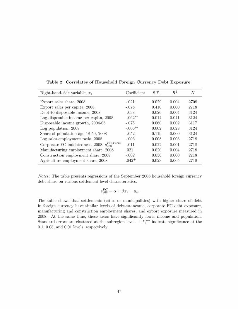
Table 2: Correlates of Household Foreign Currency Debt Exposure

Right-hand-side variable, xz Coefficient S.E. R2 N

Export sales share, 2008 -.021 0.029 0.004 2708Export sales per capita, 2008 -.078 0.410 0.000 2718Debt to disposable income, 2008 -.038 0.026 0.004 3124Log disposable income per capita, 2008 -.062∗∗ 0.014 0.041 3124Disposable income growth, 2004-08 -.075 0.060 0.002 3117Log population, 2008 -.006∗∗ 0.002 0.028 3124Share of population age 18-59, 2008 -.052 0.119 0.000 3124Log sales-employment ratio, 2008 -.006 0.008 0.003 2718

Corporate FC indebtedness, 2008, sFC,F irmz08 -.011 0.022 0.001 2718Manufacturing employment share, 2008 .021 0.020 0.004 2718Construction employment share, 2008 -.002 0.036 0.000 2718Agriculture employment share, 2008 .042+ 0.023 0.005 2718

Notes: The table presents regressions of the September 2008 household foreign currencydebt share on various settlement level characteristics:

sFCz08 = α+ βxz + uz.

The table shows that settlements (cities or municipalities) with higher share of debtin foreign currency have similar levels of debt-to-income, corporate FC debt exposure,manufacturing and construction employment shares, and export exposure measured in2008. At the same time, these areas have significantly lower income and population.Standard errors are clustered at the subregion level. +,*,** indicate significance at the0.1, 0.05, and 0.01 levels, respectively.

47

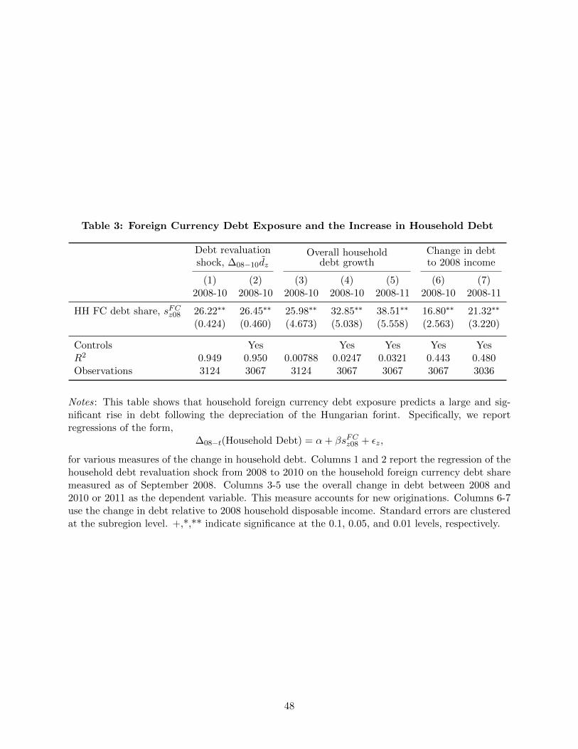
Table 3: Foreign Currency Debt Exposure and the Increase in Household Debt

Debt revaluationshock, ∆08−10dz

Overall householddebt growth

Change in debtto 2008 income

(1) (2) (3) (4) (5) (6) (7)2008-10 2008-10 2008-10 2008-10 2008-11 2008-10 2008-11

HH FC debt share, sFCz08 26.22∗∗ 26.45∗∗ 25.98∗∗ 32.85∗∗ 38.51∗∗ 16.80∗∗ 21.32∗∗

(0.424) (0.460) (4.673) (5.038) (5.558) (2.563) (3.220)

Controls Yes Yes Yes Yes YesR2 0.949 0.950 0.00788 0.0247 0.0321 0.443 0.480Observations 3124 3067 3124 3067 3067 3067 3036

Notes: This table shows that household foreign currency debt exposure predicts a large and sig-nificant rise in debt following the depreciation of the Hungarian forint. Specifically, we reportregressions of the form,

∆08−t(Household Debt) = α+ βsFCz08 + εz,

for various measures of the change in household debt. Columns 1 and 2 report the regression of thehousehold debt revaluation shock from 2008 to 2010 on the household foreign currency debt sharemeasured as of September 2008. Columns 3-5 use the overall change in debt between 2008 and2010 or 2011 as the dependent variable. This measure accounts for new originations. Columns 6-7use the change in debt relative to 2008 household disposable income. Standard errors are clusteredat the subregion level. +,*,** indicate significance at the 0.1, 0.05, and 0.01 levels, respectively.

48

Table 4: Household Debt Revaluation and Local Default Rates

∆08−10Defaultz

(1) (2) (3) (4) (5) (6)

HH FC debt share, sFCz08 7.20∗∗ 6.03∗∗ 6.30∗∗ 5.03∗∗

(0.90) (0.75) (0.73) (0.76)

HH debt revaluation, ∆08−10dz 0.22∗∗ 0.17∗∗

(0.029) (0.026)

Baseline Controls Yes Yes Yes YesExport Exposure Controls Yes Yes YesIndustry Employment Shares Yes Yes YesRegion FE (7 units) Yes YesR2 0.062 0.15 0.18 0.22 0.044 0.22Observations 3108 3051 2678 2678 3109 2678

Notes: This table shows that settlements with higher exposure to household foreign currency debtexperience a larger increase in household default rates between 2008 and 2010. Columns 1 through4 report regressions of the form

∆08−10Defaultz = α+ βsFCz08 + ΓXz + εz,

where the left-hand side is the change in the settlement default rate on housing loans. The defaultrate is measured as the fraction of loans in arears in a settlement (city or municipality). Columns5 and 6 replace the independent variable with the household debt revaluation shock, defined inequation (6) as the change in debt induced by exchange rate depreciations. Baseline controls arehousehold disposable income, household debt to income, log population, and working age andretired population shares. Export exposure controls are the export share of firm revenues andtotal firm export revenues per capita. Industry employment share controls are defined using 18one digit NACE industries (e.g., agriculture, mining, manufacturing, construction, wholesale andretail trade). Columns 4 and 6 include fixed effects for the 7 NUTS level 2 regions. Controls aremeasured in 2008. Observations are weighted by 2007 population. Standard errors are clusteredat the subregion level (175 units) based on the Ibragimov and Muller (2016) test. +,*,** indicatesignificance at the 0.1, 0.05, and 0.01 levels, respectively.

49

Table 5: Household Debt Revaluation and Household Spending

Panel A: New Auto Registrations Growth, 2008-10

(1) (2) (3) (4) (5) (6)

HH FC debt share, sFCz08 -99.5∗∗ -69.9∗∗ -78.3∗∗ -74.0∗∗

(19.5) (15.3) (14.4) (12.1)

HH debt revaluation, ∆08−10dz -3.47∗∗ -2.70∗∗

(0.64) (0.44)

Baseline Controls Yes Yes Yes YesExport Exposure Controls Yes Yes YesIndustry Employment Shares Yes Yes YesRegion FE (7 units) Yes YesR2 0.037 0.22 0.28 0.33 0.034 0.33Observations 3124 3067 2679 2679 3124 2679

Panel B: Household Electricity Usage Growth, 2008-10

(1) (2) (3) (4) (5) (6)

HH FC debt share, sFCz08 -13.1∗∗ -8.44∗ -9.25∗ -7.25∗∗

(4.33) (3.76) (3.70) (2.78)

HH debt revaluation, ∆08−10dz -0.47∗∗ -0.22∗

(0.15) (0.086)

Baseline Controls Yes Yes Yes YesExport Exposure Controls Yes Yes YesIndustry Employment Shares Yes Yes YesRegion FE (7 units) Yes YesR2 0.020 0.14 0.19 0.33 0.019 0.32Observations 3124 3067 2679 2679 3124 2679

Notes: This table presents evidence that areas with higher exposure to foreign currency debtexperience larger declines in durable spending and non-durable consumption. Panel A uses the logof the number of new auto registrations plus one as a proxy for durable spending. Panel B usesthe log of electricity consumption (in megawatt hours) as a measure of non-durable consumption.Standard errors are clustered at the subregion level (175 units) based on the Ibragimov and Muller(2016) test. +,*,** indicate significance at the 0.1, 0.05, and 0.01 levels, respectively.

50

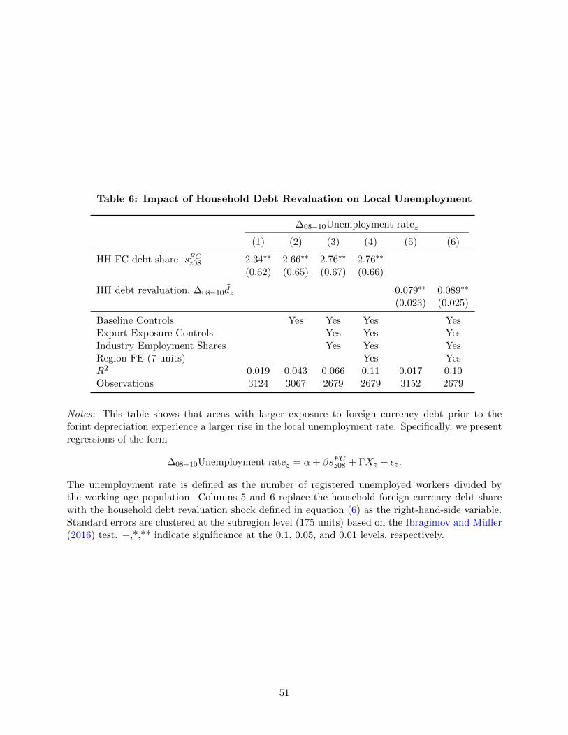
Table 6: Impact of Household Debt Revaluation on Local Unemployment

∆08−10Unemployment ratez

(1) (2) (3) (4) (5) (6)

HH FC debt share, sFCz08 2.34∗∗ 2.66∗∗ 2.76∗∗ 2.76∗∗

(0.62) (0.65) (0.67) (0.66)

HH debt revaluation, ∆08−10dz 0.079∗∗ 0.089∗∗

(0.023) (0.025)

Baseline Controls Yes Yes Yes YesExport Exposure Controls Yes Yes YesIndustry Employment Shares Yes Yes YesRegion FE (7 units) Yes YesR2 0.019 0.043 0.066 0.11 0.017 0.10Observations 3124 3067 2679 2679 3152 2679

Notes: This table shows that areas with larger exposure to foreign currency debt prior to theforint depreciation experience a larger rise in the local unemployment rate. Specifically, we presentregressions of the form

∆08−10Unemployment ratez = α+ βsFCz08 + ΓXz + εz.

The unemployment rate is defined as the number of registered unemployed workers divided bythe working age population. Columns 5 and 6 replace the household foreign currency debt sharewith the household debt revaluation shock defined in equation (6) as the right-hand-side variable.Standard errors are clustered at the subregion level (175 units) based on the Ibragimov and Muller(2016) test. +,*,** indicate significance at the 0.1, 0.05, and 0.01 levels, respectively.

51

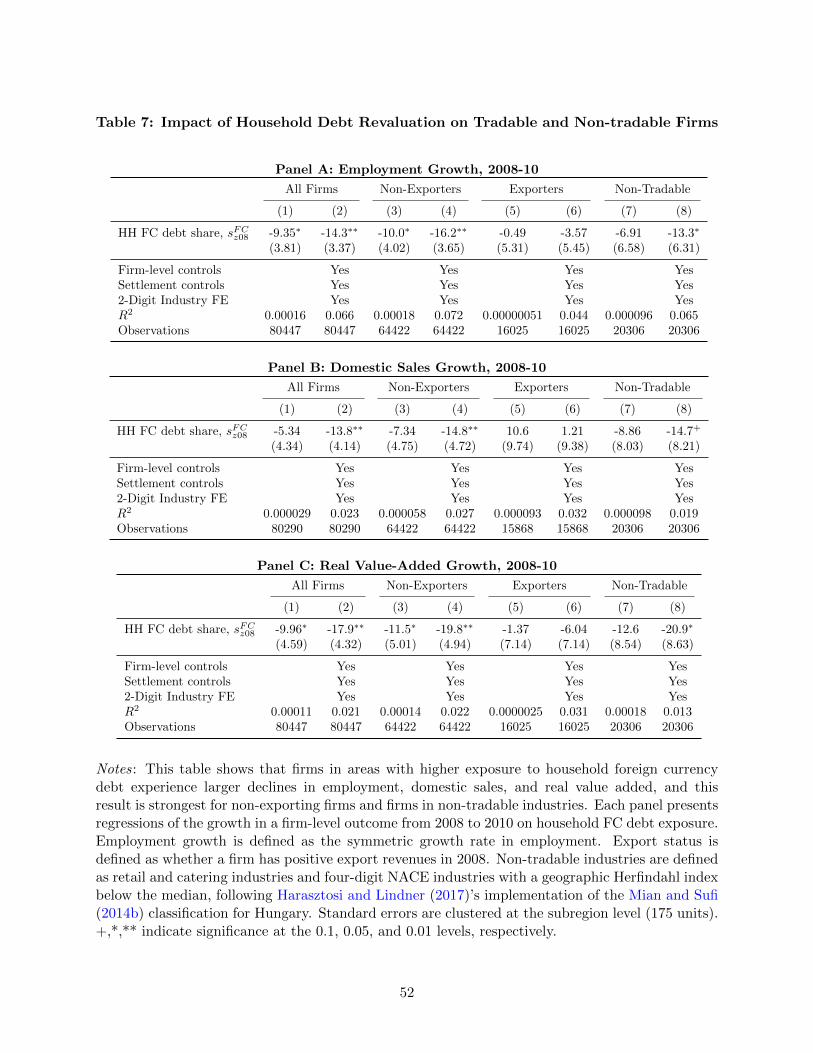
Table 7: Impact of Household Debt Revaluation on Tradable and Non-tradable Firms

Panel A: Employment Growth, 2008-10

All Firms Non-Exporters Exporters Non-Tradable

(1) (2) (3) (4) (5) (6) (7) (8)

HH FC debt share, sFCz08 -9.35∗ -14.3∗∗ -10.0∗ -16.2∗∗ -0.49 -3.57 -6.91 -13.3∗

(3.81) (3.37) (4.02) (3.65) (5.31) (5.45) (6.58) (6.31)

Firm-level controls Yes Yes Yes YesSettlement controls Yes Yes Yes Yes2-Digit Industry FE Yes Yes Yes YesR2 0.00016 0.066 0.00018 0.072 0.00000051 0.044 0.000096 0.065Observations 80447 80447 64422 64422 16025 16025 20306 20306

Panel B: Domestic Sales Growth, 2008-10

All Firms Non-Exporters Exporters Non-Tradable

(1) (2) (3) (4) (5) (6) (7) (8)

HH FC debt share, sFCz08 -5.34 -13.8∗∗ -7.34 -14.8∗∗ 10.6 1.21 -8.86 -14.7+

(4.34) (4.14) (4.75) (4.72) (9.74) (9.38) (8.03) (8.21)

Firm-level controls Yes Yes Yes YesSettlement controls Yes Yes Yes Yes2-Digit Industry FE Yes Yes Yes YesR2 0.000029 0.023 0.000058 0.027 0.000093 0.032 0.000098 0.019Observations 80290 80290 64422 64422 15868 15868 20306 20306

Panel C: Real Value-Added Growth, 2008-10

All Firms Non-Exporters Exporters Non-Tradable

(1) (2) (3) (4) (5) (6) (7) (8)

HH FC debt share, sFCz08 -9.96∗ -17.9∗∗ -11.5∗ -19.8∗∗ -1.37 -6.04 -12.6 -20.9∗

(4.59) (4.32) (5.01) (4.94) (7.14) (7.14) (8.54) (8.63)

Firm-level controls Yes Yes Yes YesSettlement controls Yes Yes Yes Yes2-Digit Industry FE Yes Yes Yes YesR2 0.00011 0.021 0.00014 0.022 0.0000025 0.031 0.00018 0.013Observations 80447 80447 64422 64422 16025 16025 20306 20306

Notes: This table shows that firms in areas with higher exposure to household foreign currencydebt experience larger declines in employment, domestic sales, and real value added, and thisresult is strongest for non-exporting firms and firms in non-tradable industries. Each panel presentsregressions of the growth in a firm-level outcome from 2008 to 2010 on household FC debt exposure.Employment growth is defined as the symmetric growth rate in employment. Export status isdefined as whether a firm has positive export revenues in 2008. Non-tradable industries are definedas retail and catering industries and four-digit NACE industries with a geographic Herfindahl indexbelow the median, following Harasztosi and Lindner (2017)’s implementation of the Mian and Sufi(2014b) classification for Hungary. Standard errors are clustered at the subregion level (175 units).+,*,** indicate significance at the 0.1, 0.05, and 0.01 levels, respectively.

52

Table 8: Impact of Household Debt Revaluation on Local Unemployment: Robustness

(1) (2) (3) (4) (5)

Panel A: Alternative Measures of Household FC Debt Exposure

HH debt to inc. revaluation, ∆08−10dIncz 0.079∗∗

(0.024)

Fraction of loans in FC, fFCz08 3.41∗∗

(0.70)

FC loans per adult (std.) 0.61∗∗

(0.090)

LC loans per adult (std.) -0.099(0.10)

FC debt share, mortgages only 1.95∗∗

(0.51)

Controls Yes Yes Yes Yes YesR2 0.032 0.049 0.067 0.021 0.040Observations 3067 3067 3067 3067 3023

Panel B: Weights, Subsamples, and Subregional Aggregation

HH FC debt share, sFCz08 1.75∗∗ 1.61∗∗ 2.26∗∗ 3.85∗∗ 1.90∗

(0.51) (0.59) (0.74) (1.37) (0.74)

Controls Yes Yes Yes Yes YesSample Full 50% smallest 50% largest Largest cities 175 subreg.Weights None None None None Pop.R2 0.055 0.061 0.056 0.067 0.073Observations 3067 1534 1533 306 175

Panel C: Additional Specification Checks, Estimation Period: 2006-2011

HH FC debt share, sFCz08 × POSTt 2.03∗∗ 2.21∗∗ 2.01∗∗ 1.89∗∗ 1.47∗∗

(0.57) (0.58) (0.57) (0.40) (0.37)

Unemployment rate in 2008 × POSTt -0.092∗∗

(0.020)

Default rate in 2008:9 × POSTt 0.017(0.026)

SD of unemp. rate, 1995-2007 × POSTt -0.19∗

(0.094)

POSTt 2.13+ 3.40∗∗ 2.63∗ 2.90∗∗ 1.25(1.11) (1.16) (1.16) (1.03) (0.97)

Controls×POST Yes Yes Yes Yes YesSettlement FE Yes Yes Yes Yes YesSubregion time trends Yes YesRegion (20 units)-POST FE YesR2 0.63 0.63 0.63 0.71 0.73Observations 18402 18402 18402 18402 18402

Notes: This table shows that the effect of household foreign currency debt exposure on local unem-ployment is robust to a variety of specification and sample checks. The dependent variable in panelsA and B is the change in the local unemployment rate from 2008 to 2010. In panel C we estimatea difference-in-differences specification using annual data from 2006 to 2011, where POSTt equals 1in years 2009 onward. This specification allows us to control for 175 subregion specific time trends.Standard errors are clustered at the subregion level (175 units) based on the Ibragimov and Muller(2016) test. +,*,** indicate significance at the 0.1, 0.05, and 0.01 levels, respectively.

53

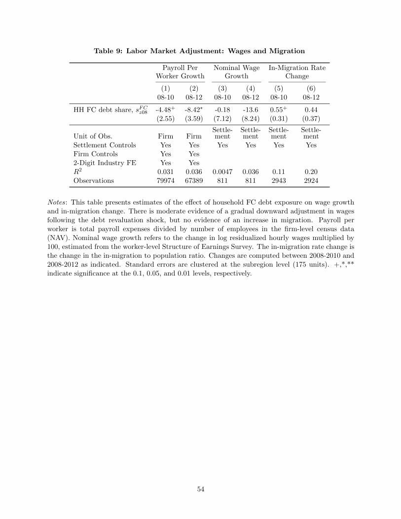
Table 9: Labor Market Adjustment: Wages and Migration

Payroll PerWorker Growth

Nominal WageGrowth

In-Migration RateChange

(1) (2) (3) (4) (5) (6)08-10 08-12 08-10 08-12 08-10 08-12

HH FC debt share, sFCz08 -4.48+ -8.42∗ -0.18 -13.6 0.55+ 0.44(2.55) (3.59) (7.12) (8.24) (0.31) (0.37)

Unit of Obs. Firm FirmSettle-ment

Settle-ment

Settle-ment

Settle-ment

Settlement Controls Yes Yes Yes Yes Yes YesFirm Controls Yes Yes2-Digit Industry FE Yes YesR2 0.031 0.036 0.0047 0.036 0.11 0.20Observations 79974 67389 811 811 2943 2924

Notes: This table presents estimates of the effect of household FC debt exposure on wage growthand in-migration change. There is moderate evidence of a gradual downward adjustment in wagesfollowing the debt revaluation shock, but no evidence of an increase in migration. Payroll perworker is total payroll expenses divided by number of employees in the firm-level census data(NAV). Nominal wage growth refers to the change in log residualized hourly wages multiplied by100, estimated from the worker-level Structure of Earnings Survey. The in-migration rate change isthe change in the in-migration to population ratio. Changes are computed between 2008-2010 and2008-2012 as indicated. Standard errors are clustered at the subregion level (175 units). +,*,**indicate significance at the 0.1, 0.05, and 0.01 levels, respectively.

54

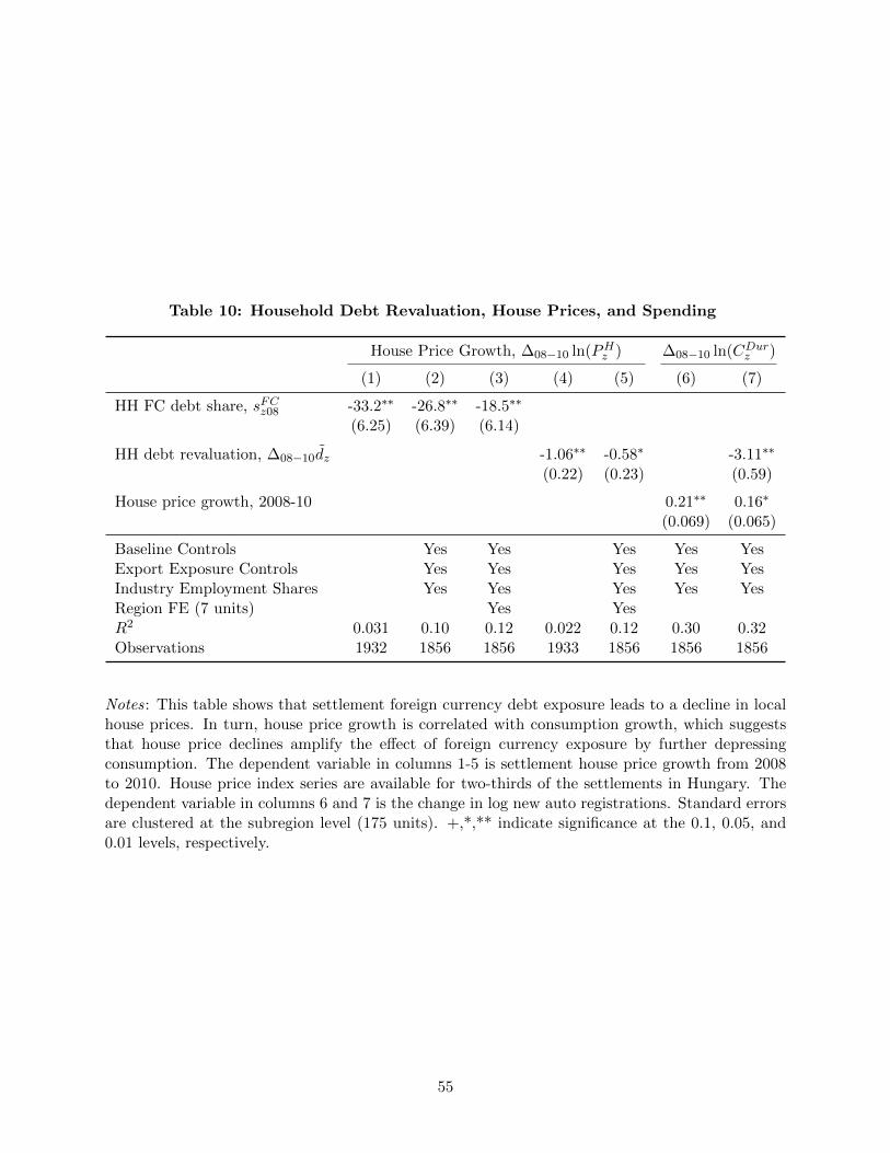
Table 10: Household Debt Revaluation, House Prices, and Spending

House Price Growth, ∆08−10 ln(PHz ) ∆08−10 ln(CDurz )

(1) (2) (3) (4) (5) (6) (7)

HH FC debt share, sFCz08 -33.2∗∗ -26.8∗∗ -18.5∗∗

(6.25) (6.39) (6.14)

HH debt revaluation, ∆08−10dz -1.06∗∗ -0.58∗ -3.11∗∗

(0.22) (0.23) (0.59)

House price growth, 2008-10 0.21∗∗ 0.16∗

(0.069) (0.065)

Baseline Controls Yes Yes Yes Yes YesExport Exposure Controls Yes Yes Yes Yes YesIndustry Employment Shares Yes Yes Yes Yes YesRegion FE (7 units) Yes YesR2 0.031 0.10 0.12 0.022 0.12 0.30 0.32Observations 1932 1856 1856 1933 1856 1856 1856

Notes: This table shows that settlement foreign currency debt exposure leads to a decline in localhouse prices. In turn, house price growth is correlated with consumption growth, which suggeststhat house price declines amplify the effect of foreign currency exposure by further depressingconsumption. The dependent variable in columns 1-5 is settlement house price growth from 2008to 2010. House price index series are available for two-thirds of the settlements in Hungary. Thedependent variable in columns 6 and 7 is the change in log new auto registrations. Standard errorsare clustered at the subregion level (175 units). +,*,** indicate significance at the 0.1, 0.05, and0.01 levels, respectively.

55

Table 11: Financial Spillovers: Loan-Level Evidence from Defaults

LC and FCHousing Loans

LCBorrower

FCBorrower

(1) (2) (3) (4) (5) (6)

Foreign currency loan, FCi 2.63∗∗ 2.21∗∗ 11.9∗∗ 2.59∗∗

(0.16) (0.17) (0.97) (0.16)

Local HH FC debt share, sFCz,−b,08 3.08∗∗ 3.32∗∗ 3.55∗∗

(0.80) (1.02) (0.98)

FCi ×High Leverage Indicatorb 0.87∗∗

(0.17)

FCi ×Maturity (years)i -0.52∗∗

(0.039)

Loan Controls Yes Yes Yes Yes Yes YesBorrower Controls Yes Yes Yes Yes Yes YesSettlement Controls Yes Yes Yes Yes Yes YesR2 0.012 0.013 0.058 0.012 0.013 0.0065Observations 650193 650193 650175 650193 215394 434799

Notes: This table presents loan-level regressions of the change in default status from 2008 to 2010on an indicator for whether a loan is in foreign currency (FCi) and foreign currency exposure inthe borrower’s settlement of residence, excluding borrower b (sFCz,−b,08):

∆08−10Defaulti,b,z = β0 + β1FCi + β2sFCz,−b,08 +XL

i ΓL +XBb ΓB +XS

z ΓS + εiz

Columns 1-3 show that foreign currency loans are more likely to default, and this effect is strongerfor borrowers with higher leverage and shorter maturity loans. Column 4 shows that both theloan’s own currency denomination and local foreign currency debt exposure predict an increasedprobability of default. Columns 5 and 6 split the sample into local and foreign currency borrowersand show that higher local exposure to foreign currency debt predicts an increased probabilityof default for both local and foreign currency borrowers. Local currency borrowers are definedas borrowers who have no individual exposure to FC debt. Loan controls are a loan type fixedeffect (mortgage or HE) and a quadratic in log loan size. Borrower controls are the total numberof mortgage and HE loans, log total borrower debt in 2008, and five-year age bin fixed effects.Settlement controls are log population, debt-to-income, disposable income per capita, fraction ofthe population age 18 to 59 and fraction age 60 or more, export revenue share, exports per capita,one-digit industry employment shares, and fixed effects for seven major regions. Controls aremeasured in 2008. Standard errors are clustered at the subregion level (175 units). +,*,** indicatesignificance at the 0.1, 0.05, and 0.01 levels, respectively.

56

Table 12: Firm FC Debt, Household FC Debt, and Firm-Level Outcomes from 2008to 2010

Inv.-CapitalChange, 08-10

SalesGrowth, 08-10

EmploymentGrowth, 08-10

(1) (2) (3) (4) (5) (6) (7)

Firm FC debt share -10.0∗∗ -11.4∗∗ 1.76∗ 2.64∗∗ 4.05∗∗ 0.77(1.27) (1.34) (0.68) (0.68) (0.50) (0.48)

HH FC debt share, sFCz08 -7.05 -13.4∗∗ -14.1∗∗ -13.4∗∗

(4.39) (4.11) (3.36) (3.71)

sFCz08 × Firm has FC debt -3.48(5.42)

Firm has FC debt 3.39(3.57)

Firm Controls Yes Yes Yes YesSettlement Controls Yes Yes Yes Yes2-Digit Industry FE Yes Yes Yes YesR2 0.0012 0.0084 0.000065 0.028 0.00055 0.066 0.066Observations 80447 80447 80447 80447 80447 80447 80447

Notes: This table presents firm-level regressions comparing the effects of local household FC debtand firm FC debt on the evolution of firm outcomes from 2008 to 2010. The dependent variablesare the change in the investment to lagged capital ratio (columns 1-2), firm sales growth (columns3-4), and employment growth (columns 5-7). Growth rates are computed using the symmetricgrowth rate to mitigate the influence of outliers and allow for zeros. Firms with a higher fraction ofFC debt experience falling investment, but stronger sales growth and no difference in employmentgrowth. Household foreign currency debt exposure robustly predicts falling sales and employment.Appendix Table A.11 shows that these results are similar when measuring firm foreign currencyexposure using FC debt to assets ratio. Standard errors are clustered at the subregion level (175units). +,*,** indicate significance at the 0.1, 0.05, and 0.01 levels, respectively.

57

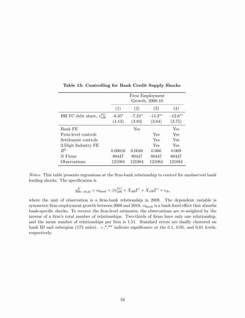
Table 13: Controlling for Bank Credit Supply Shocks

Firm EmploymentGrowth, 2008-10

(1) (2) (3) (4)

HH FC debt share, sFCz08 -9.35∗ -7.24+ -14.3∗∗ -12.6∗∗

(4.13) (3.83) (3.84) (3.75)

Bank FE Yes YesFirm-level controls Yes YesSettlement controls Yes Yes2-Digit Industry FE Yes YesR2 0.00016 0.0040 0.066 0.069N Firms 80447 80447 80447 80447Observations 121084 121084 121084 121084

Notes: This table presents regressions at the firm-bank relationship to control for unobserved banklending shocks. The specification is

gE08−10,ib = αbank + βsFCz08 +Xi08Γi +Xz08Γz + εib,

where the unit of observation is a firm-bank relationship in 2008. The dependent variable issymmetric firm employment growth between 2008 and 2010. αbank is a bank fixed effect that absorbsbank-specific shocks. To recover the firm-level estimates, the observations are re-weighted by theinverse of a firm’s total number of relationships. Two-thirds of firms have only one relationship,and the mean number of relationships per firm is 1.51. Standard errors are dually clustered onbank ID and subregion (175 units). +,*,** indicate significance at the 0.1, 0.05, and 0.01 levels,respectively.

58

Figure 1: Household Credit Expansion in Domestic and Foreign Currency

5

10

15

20

25

30

35

40H

ouse

hold

deb

t-to-

GD

P (%

)

2000q1 2003q1 2006q1 2009q1 2012q1

(a) Household debt-to-GDP ratio (%)

0

5

10

15

20

25

Hou

sing

deb

t-to-

GD

P (%

)

2000q1 2003q1 2006q1 2009q1 2012q1

Foreign CurrencyDomestic Currency

(b) Housing debt in domestic and foreign currency

Notes: Panel (a) shows the increase in total household debt-to-GDP from the BIS’s “Long seriesin credit to the private sector” database. Panel (b) depicts the evolution of mortgage and homeequity debt in domestic and foreign currency from the National Bank of Hungary. The verticaldashed line represents September 2008, the month prior to the forint depreciation.

59

Figure 2: Household Debt Revaluation Shock Induced by the Forint Depreciation

Oct. 2008

90

100

110

120

130

140

150

160

Exch

ange

rate

, 200

5m1=

100

2000m1 2002m1 2004m1 2006m1 2008m1 2010m1 2012m1 2014m1

Euro Swiss franc

(a) Nominal exchange rate relative to euro and Swiss franc

05

1015

Hou

sing

deb

t sho

ck re

lativ

e to

200

8 di

sp. i

ncom

e (%

)

2009m1 2010m1 2011m1 2012m1 2013m1 2014m1

(b) Household debt-revaluation induced by the depreciation, as a per-centage of disposable income

Notes: Panel (a) shows the evolution of the forint-euro and forint-Swiss franc exchange rates. Thefigure shows that a de facto ±5% crawling band target up to 2008:2 was followed by a suddendepreciation in October 2008. The forint depreciated further relative to the Swiss franc duringthe European debt crisis in 2010. Panel (b) presents the household debt-revaluation shock inducedby the depreciation computed as the difference between the value of 2008:9 outstanding housingdebt at market exchange rates and housing debt assuming exchange rates remain at their 2008:9value, scaled by 2008 disposable income. The forint depreciation led to an unanticipated increasein housing debt of 5-10% in 2009 and 10% by mid-2010.

60

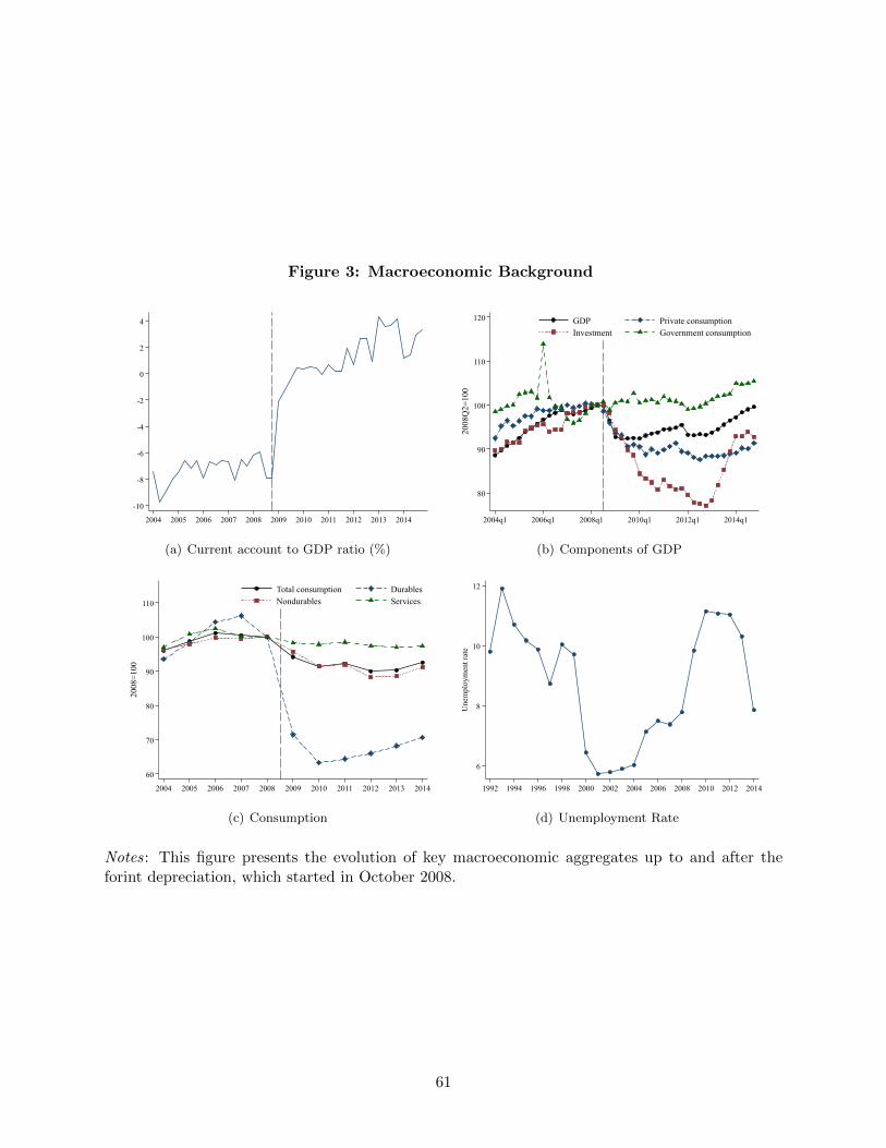
Figure 3: Macroeconomic Background

-10

-8

-6

-4

-2

0

2

4

2004 2005 2006 2007 2008 2009 2010 2011 2012 2013 2014

(a) Current account to GDP ratio (%)

80

90

100

110

120

2008

Q2=

100

2004q1 2006q1 2008q1 2010q1 2012q1 2014q1

GDP Private consumptionInvestment Government consumption

(b) Components of GDP

60

70

80

90

100

110

2008

=100

2004 2005 2006 2007 2008 2009 2010 2011 2012 2013 2014

Total consumption DurablesNondurables Services

(c) Consumption

6

8

10

12

Une

mpl

oym

ent r

ate

1992 1994 1996 1998 2000 2002 2004 2006 2008 2010 2012 2014

(d) Unemployment Rate

Notes: This figure presents the evolution of key macroeconomic aggregates up to and after theforint depreciation, which started in October 2008.

61

Figure 4: Distribution of Household Foreign Currency Debt Exposure

FC housing debt share: 2008m9(.8627352,1.000037](.7902051,.8627352](.7474093,.7902051](.7124748,.7474093](.6742026,.7124748](.6511398,.6742026](.6178734,.6511398](.5734839,.6178734](.4992683,.5734839][-5.87e-08,.4992683]No data

Note: this figure shows the geographical distribution of the share of FC housing debt in total housing (mortgage and HE) debt in September 2008.

(a) Geographic Distribution of Household FC Debt Exposure

0.1

.2.3

.4.5

.6.7

.8.9

Ave

rage

FC

sha

re o

f hou

seho

ld d

ebt

1 2 3 4 5 6 7 8 11 12 13 14 15 16 17 18 19 20

(b) Variation in FC Debt Exposure

Notes: Panel (a) presents a map of the household FC debt share across 3124 settlements in Hungary.The map shows that there is variation both within and across regions in the share of household debtdenominated in FC. Panel (b) sorts settlements into 20 equal population bins by the householdforeign currency debt share measured in September 2008, sFC08 , and presents the average of sFC08

within each bin. The figure shows there is substantial variation in exposure going from the lowestto the highest quantiles.

62

Figure 5: Household Foreign Currency Debt Exposure and Local Default Rates

05

1015

2025

30C

oeff

icie

nt e

stim

ate

2008q1 2009q1 2010q1 2011q1 2012q1 2013q1 2014q1 2015q1

Notes: This figure presents estimates of {βq} from

Defaultzt = αz + γt +∑

q 6=2008Q1

βq(sFCz08 · 1q=t) + εzt.

The outcome variable is the settlement default rate on housing loans, defined as the fraction ofhousing loans in default. Coefficients are multiplied by 100. The estimation period is 2008Q1, asthis is the first period that default status is available. For reference, the aggregate default rate onhousing loans increased from 0.9% in 2008:9 to 4.7% in 2010:9 and 13.9% in 2014:9. Error barsrepresent 95% confidence intervals from standard errors clustered at the subregion level based onthe Ibragimov and Muller (2016) test for the appropriate level of clustering.

63

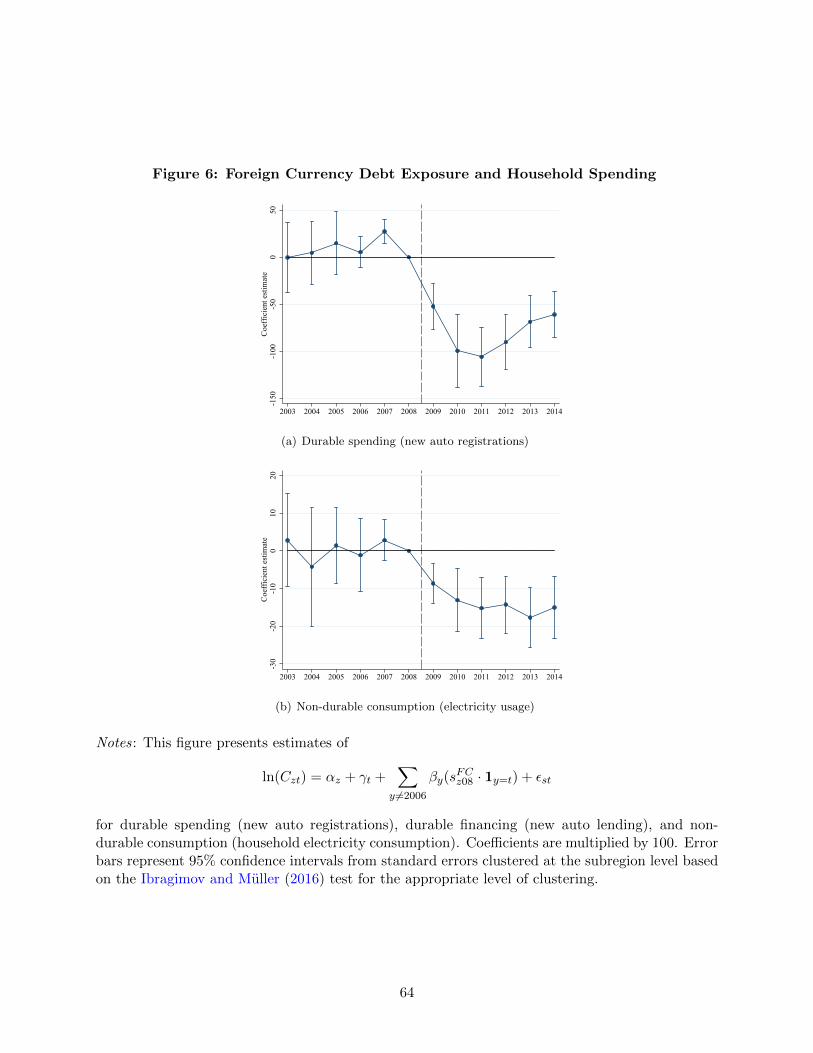
Figure 6: Foreign Currency Debt Exposure and Household Spending

-150

-100

-50

050

Coe

ffic

ient

est

imat

e

2003 2004 2005 2006 2007 2008 2009 2010 2011 2012 2013 2014

(a) Durable spending (new auto registrations)

-30

-20

-10

010

20C

oeff

icie

nt e

stim

ate

2003 2004 2005 2006 2007 2008 2009 2010 2011 2012 2013 2014

(b) Non-durable consumption (electricity usage)

Notes: This figure presents estimates of

ln(Czt) = αz + γt +∑

y 6=2006

βy(sFCz08 · 1y=t) + εst

for durable spending (new auto registrations), durable financing (new auto lending), and non-durable consumption (household electricity consumption). Coefficients are multiplied by 100. Errorbars represent 95% confidence intervals from standard errors clustered at the subregion level basedon the Ibragimov and Muller (2016) test for the appropriate level of clustering.

64

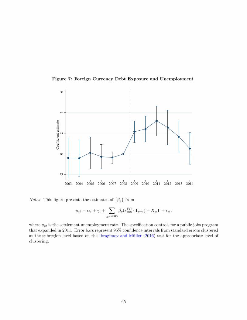
Figure 7: Foreign Currency Debt Exposure and Unemployment

-20

24

6C

oeff

icie

nt e

stim

ate

2003 2004 2005 2006 2007 2008 2009 2010 2011 2012 2013 2014

Notes: This figure presents the estimates of {βy} from

uzt = αz + γt +∑

y 6=2006

βy(sFCz08 · 1y=t) +XztΓ + εst,

where uzt is the settlement unemployment rate. The specification controls for a public jobs programthat expanded in 2011. Error bars represent 95% confidence intervals from standard errors clusteredat the subregion level based on the Ibragimov and Muller (2016) test for the appropriate level ofclustering.

65

Figure 8: Placebo Test: 1998 Russian Financial Crisis

-20

24

6C

oeff

icie

nt e

stim

ate

1995 1996 1997 1998 1999 2000 2001

Notes: This figure uses the second half of the 1990s as a placebo sample. Figure 3 shows thatunemployment in Hungary rose around the 1998 Russian Financial Crisis, and then subsequentlyrecovered. This figure presents estimates of the following specification for the period 1995-2001,where 1997 is the omitted year,

uzt = αz + γt +∑y

βy{sFCz08 · 1y=t}+ εzt.

For the late 1990s placebo sample the coefficients {βy} are precisely estimated and not significantlydifferent from zero.

66

Figure 9: Foreign Currency Debt Exposure and House Prices

-100

-80

-60

-40

-20

020

4060

Coe

ffic

ient

est

imat

e

2005

2006

2007

2008

2009

2010

2011

2012

2013

2014

Notes: This figure presents the estimates of {βy} from

ln(PHzt ) = αz + γt +∑

y 6=2008

[βy(sFCz08 · 1y=t) + Γy(Xz08 · 1y=t)] + εst,

where ln(PHzt ) is (100 times) the log of the settlement home price index. The specification includescontrols corresponding to of Table 10 column 3 interacted with year dummies, as Table 10 revealsthat the estimates are sensitive to the inclusion of these controls (see Figure A.3 for the estimateswithout controls). Error bars represent 95% confidence intervals computed from standard errorsclustered at the subregion level. House prices are only available for 187 major settlements prior to2007, so the estimated effect from 2005 and 2006 to 2008 is more uncertain.

67

A Appendix Tables and Figures

Table A.1: Initial Banking Density and Household Foreign Currency Debt

(1) (2) (3) (4)

DTI2008

LC DTI2008

FC DTI2008

HH FC debtshare, sFCz08

Log banking density in 1995 -0.064 0.042 -0.12∗ -0.12∗∗

(0.064) (0.032) (0.055) (0.038)

Baseline Controls Yes Yes Yes YesExport Exposure Controls Yes Yes Yes YesIndustry Employment Shares Yes Yes Yes YesRegion FE (7 units) Yes Yes Yes YesR2 0.30 0.31 0.24 0.30Observations 2679 2679 2679 2679

Notes: This table presents regressions of various measures of households’ debt portfolios in Septem-ber 2008 on the log retail banking density in 1995. Banking density is defined as the number ofbank branches per capita. Settlements with a higher initial banking density (of domestic banks)have lower overall debt-to-income in 2008 (column 1), higher debt-to-income in local currency (col-umn 2), lower debt-to-income in foreign currency (column 3), and therefore a lower share of debtin foreign currency (column 4). Standard errors are clustered at the subregion level (175 units).+,*,** indicate significance at the 0.1, 0.05, and 0.01 levels, respectively.

68

Table A.2: Robustness: Household Debt Revaluation to Income Shock

Panel A: Settlement Level Outcomes

Change from 2008 to 2010

(1) (2) (3) (4) (5)

DefaultAutoReg.

AutoFin.

Non-dur.Cons.

Unemp.Rate

HH debt to inc. revaluation, ∆08−10dIncz 0.099∗∗ -2.50∗∗ -0.67+ -0.30∗ 0.072∗∗

(0.026) (0.54) (0.34) (0.12) (0.022)

Baseline Controls Yes Yes Yes Yes YesExport Exposure Controls Yes Yes Yes Yes YesIndustry Employment Shares Yes Yes Yes Yes YesR2 0.20 0.32 0.054 0.33 0.095Observations 2678 2679 2615 2679 2679

Panel B: Firm Level Outcomes

Change from 2008 to 2010

(1) (2) (3) (4) (5) (6)

Empl.Domestic

SalesReal Val.

AddedEmpl.

Non-Exp.Empl.

ExportersEmpl.

Non-trad.

HH debt revaluation -0.46∗∗ -0.57∗∗ -0.71∗∗ -0.50∗∗ -0.14 -0.49∗

rel. to income, ∆08−10dIncz (0.14) (0.15) (0.16) (0.14) (0.23) (0.21)

Firm Controls Yes Yes Yes Yes Yes YesSettlement Controls Yes Yes Yes Yes Yes Yes2-Digit Industry FE Yes Yes Yes Yes Yes YesR2 0.066 0.023 0.021 0.072 0.044 0.065Observations 80447 80290 80447 64422 16025 20306

Notes: Panel A shows that the main settlement level results are robust to using the household debtrevaluation to income shock defined in equation (7). Panel B reports firm level regressions of themain firm level outcomes on the household debt revaluation to income measure. Standard errorsare clustered at the subregion level (175 units). +,*,** indicate significance at the 0.1, 0.05, and0.01 levels, respectively.

69

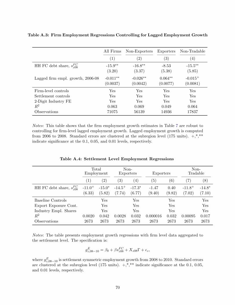
Table A.3: Firm Employment Regressions Controlling for Lagged Employment Growth

All Firms Non-Exporters Exporters Non-Tradable

(1) (2) (3) (4)

HH FC debt share, sFCz08 -15.9∗∗ -16.8∗∗ -8.53 -15.5∗∗

(3.20) (3.37) (5.38) (5.85)

Lagged firm empl. growth, 2006-08 -0.011∗∗ -0.026∗∗ 0.064∗∗ -0.015+

(0.0037) (0.0042) (0.0077) (0.0081)

Firm-level controls Yes Yes Yes YesSettlement controls Yes Yes Yes Yes2-Digit Industry FE Yes Yes Yes YesR2 0.063 0.069 0.049 0.064Observations 71075 56139 14936 17837

Notes: This table shows that the firm employment growth estimates in Table 7 are robust tocontrolling for firm-level lagged employment growth. Lagged employment growth is computedfrom 2006 to 2008. Standard errors are clustered at the subregion level (175 units). +,*,**indicate significance at the 0.1, 0.05, and 0.01 levels, respectively.

Table A.4: Settlement Level Employment Regressions

TotalEmployment

Non-Exporters Exporters

Non-Tradable

(1) (2) (3) (4) (5) (6) (7) (8)

HH FC debt share, sFCz08 -11.0+ -15.0∗ -14.5+ -17.3∗ -1.47 0.40 -11.8+ -14.8∗

(6.33) (5.82) (7.74) (6.77) (9.40) (9.82) (7.02) (7.10)

Baseline Controls Yes Yes Yes YesExport Exposure Cont. Yes Yes Yes YesIndustry Empl. Shares Yes Yes Yes YesR2 0.0020 0.042 0.0028 0.032 0.000016 0.032 0.00095 0.017Observations 2673 2673 2673 2673 2673 2673 2673 2673

Notes: The table presents employment growth regressions with firm level data aggregated tothe settlement level. The specification is:

gEz,08−10 = β0 + βsFCz08 +Xz08Γ + εz,

where gEz,08−10 is settlement symmetric employment growth from 2008 to 2010. Standard errorsare clustered at the subregion level (175 units). +,*,** indicate significance at the 0.1, 0.05,and 0.01 levels, respectively.

70

Table A.5: Robustness to Omitted Variables Bias

SpecificationEstimatew\o cont.

Estimatew\cont. R2 R2 2.2 · R2 Identified Set

Default 7.2 5.03 0.06 0.22 0.48 5.03 1.40Auto registration -99.5 -74 0.04 0.33 0.73 -74.00 -39.54Electricity cons. -13.1 -7.25 0.02 0.33 0.73 -7.25 0.22Unemployment 2.34 2.76 0.02 0.11 0.24 2.76 3.37Default spillover 5.38 3.88 0.01 0.16 0.35 3.88 2.02House prices -33.2 -18.5 0.03 0.12 0.26 -18.50 5.28

Notes: This table presents the identified sets computed using the methodology developed by Oster

(2016) and Altonji et al. (2005). The identified set is computed at[β − δ(β − β)R

2max−R2

R2−R2, β], where

β and R2 are from the short regression, β and R2 are from the long regression, and δ = 1 andR2max = 2.2R2, based on the recommendation in Oster (2016). For all outcomes except non-durable

(electricity) consumption and house prices, we can reject that the estimates are driven by omittedvariable bias under an assumption of proportional selection on observables and unobservables.

71

Table A.6: Banking Shift-Share Instrument

Panel A: Settlement Level Outcomes

Firststage IV: Change from 2008 to 2010

(1) (2) (3) (4) (5) (6)

sFCz08 DefaultAuto

spendingElectr.usage

Unem.rate

Houseprices

Shift-share FC debt shock, Vz08 0.73∗∗

(0.047)

sFCz08 5.04∗∗ -131.1∗∗ 2.72 4.11∗∗ -16.7(1.19) (25.1) (4.69) (1.04) (10.4)

Baseline Controls Yes Yes Yes Yes Yes YesExport Exposure Controls Yes Yes Yes Yes Yes YesIndustry Employment Shares Yes Yes Yes Yes Yes YesRegion FE (7 units) Yes Yes Yes Yes Yes YesR2 0.47 0.22 0.31 0.32 0.097 0.11Observations 2677 2677 2677 2677 2677 2334

Panel B: Firm Level Outcomes

IV: Change from 2008 to 2010

(1) (2) (3) (4) (5) (6)

Empl.Domestic

SalesReal Val.

AddedEmpl.

Non-Exp.Empl.Exp.

Empl.Non-trad.

HH FC debt share, sFCz08 -14.4∗∗ -16.4∗∗ -23.5∗∗ -16.2∗∗ -1.21 -6.48(4.94) (5.54) (6.31) (5.58) (9.67) (8.62)

Firm Controls Yes Yes Yes Yes Yes YesSettlement Controls Yes Yes Yes Yes Yes Yes2-Digit Industry FE Yes Yes Yes Yes Yes YesR2 0.066 0.022 0.021 0.072 0.044 0.065Observations 80447 80290 80447 64422 16025 20306

Notes: This table shows that the main results are robust to instrumenting the household FCdebt share with an instrument constructed using banks’ local market shares and their propensityto lend in domestic and foreign currency, defined in equation (8). Standard errors are clusteredat the subregion level (175 units). +,*,** indicate significance at the 0.1, 0.05, and 0.01 levels,respectively.

72

Table A.7: Labor Market Adjustment: Wages and Migration without Controls

Payroll PerWorker Growth

Nominal WageGrowth

In-Migration RateChange

(1) (2) (3) (4) (5) (6)08-10 08-12 08-10 08-12 08-10 08-12

HH FC debt share, sFCz08 -4.85+ -5.26 2.68 -2.33 1.02∗∗ 2.01∗∗

(2.49) (3.97) (6.59) (8.68) (0.36) (0.49)

Unit of Obs. Firm Firm Settl. Settl. Settl. Settl.R2 0.0045 0.0064 0.00026 0.00016 0.0049 0.015Observations 79974 67389 811 811 2943 2924

Notes: This table presents the regressions in Table 9 without control variables. Standard errorsare clustered at the subregion level (175 units). +,*,** indicate significance at the 0.1, 0.05, and0.01 levels, respectively.

Table A.8: Household and Firm FC Debt Exposure by Firm Size

All FirmsSmall

(3 to 9)Medium

(10 to 50)Large(≥ 51)

(1) (2) (3) (4)

HH FC debt share, sFCz08 0.0094 0.028 -0.019 -0.051(0.034) (0.032) (0.042) (0.11)

R2 0.0000048 0.000051 0.000017 0.000092Observations 80447 54273 21371 4803

Notes: The dependent variable is the firm level foreign currency debt share in 2008. Standarderrors are clustered at the subregion level (175 units). +,*,** indicate significance at the 0.1, 0.05,and 0.01 levels, respectively.

73

Table A.9: Effect of Household Debt Revaluation on Employment Growth: Effects byFirm Size

Small (3 to 9) Medium (10 to 50) Large (≥ 51)

(1) (2) (3) (4) (5) (6)

HH FC debt share, sFCz08 -8.57+ -12.8∗∗ -10.8+ -18.2∗∗ -10.4 -14.4+

(5.01) (4.63) (5.57) (5.06) (8.47) (8.29)

Firm-level controls Yes Yes YesSettlement controls Yes Yes Yes2-Digit Industry FE Yes Yes YesR2 0.00013 0.071 0.00023 0.075 0.00027 0.055Observations 54273 54273 21371 21371 4803 4803

Notes: This table reports firm level regressions by firm size of symmetric employment growth from2008 to 2010 on the local household FC debt share. Standard errors are clustered at the subregionlevel (175 units). +,*,** indicate significance at the 0.1, 0.05, and 0.01 levels, respectively.

Table A.10: Determinants of Firm Foreign Currency Financing

Right-hand-side variable Coefficient S.E. R2 N

Log employment, 2008 0.039∗∗ .002 0.019 80447Log sales per worker, 2008 0.026∗∗ .001 0.011 80447Employment growth, 2004-08 0.016∗∗ .002 0.001 62219Export sales share, 2008 0.140∗∗ .014 0.008 80447Exporter 0.076∗∗ .008 0.011 80447Manufacturing 0.052∗∗ .003 0.005 80447

Notes: This table presents firm-level univariate regressions of a firm’s foreign currency debt shareon a firm characteristic:

(Firm FC debt share)i08 = α+ βxi + ui.

Firms with a higher share of debt in foreign currency tend to be larger, faster growing, more exportintensive, and more likely to be in manufacturing. Standard errors are clustered at the subregionlevel (175 units). +,*,** indicate significance at the 0.1, 0.05, and 0.01 levels, respectively.

74

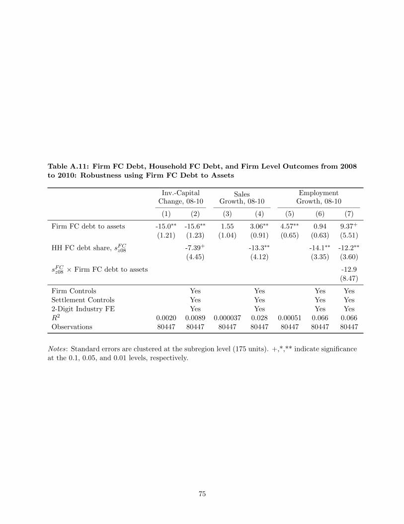
Table A.11: Firm FC Debt, Household FC Debt, and Firm Level Outcomes from 2008to 2010: Robustness using Firm FC Debt to Assets

Inv.-CapitalChange, 08-10

SalesGrowth, 08-10

EmploymentGrowth, 08-10

(1) (2) (3) (4) (5) (6) (7)

Firm FC debt to assets -15.0∗∗ -15.6∗∗ 1.55 3.06∗∗ 4.57∗∗ 0.94 9.37+

(1.21) (1.23) (1.04) (0.91) (0.65) (0.63) (5.51)

HH FC debt share, sFCz08 -7.39+ -13.3∗∗ -14.1∗∗ -12.2∗∗

(4.45) (4.12) (3.35) (3.60)

sFCz08 × Firm FC debt to assets -12.9(8.47)

Firm Controls Yes Yes Yes YesSettlement Controls Yes Yes Yes Yes2-Digit Industry FE Yes Yes Yes YesR2 0.0020 0.0089 0.000037 0.028 0.00051 0.066 0.066Observations 80447 80447 80447 80447 80447 80447 80447

Notes: Standard errors are clustered at the subregion level (175 units). +,*,** indicate significanceat the 0.1, 0.05, and 0.01 levels, respectively.

75

Figure A.1: Correlation of Household Foreign Currency Exposure with Key Observ-ables

0.2

.4.6

.8Ex

port

Shar

e of

Tot

al F

irm R

even

ues,

2008

.4 .5 .6 .7 .8 .9Household FC Debt Exposure, 2008

(a) Export exposure

.3.4

.5.6

Deb

t to

Dis

posa

ble

Inco

me,

200

8

.2 .4 .6 .8 1Household FC Debt Exposure, 2008

(b) Debt to disposable income

13.8

1414

.214

.414

.6Lo

g D

ispo

sabl

e In

com

e, 2

008

.2 .4 .6 .8 1Household FC Debt Exposure, 2008

(c) Disposable income per capita

0.2

.4.6

.8M

anuf

actu

ring

Empl

oym

ent S

hare

, 200

8

.4 .5 .6 .7 .8 .9Household FC Debt Exposure, 2008

(d) Manufacturing employment share

Notes: These figures present binned bivariate means at the settlement level of key observablesagainst the September 2008 household foreign currency debt share, sFCz08.

76

Figure A.2: Foreign Currency Debt Exposure and Settlement Employment

-60

-40

-20

020

40C

oeff

icie

nt e

stim

ate

2003 2004 2005 2006 2007 2008 2009 2010 2011 2012 2013 2014

(a) Total Employment

-60

-40

-20

020

40C

oeff

icie

nt e

stim

ate

2003 2004 2005 2006 2007 2008 2009 2010 2011 2012 2013 2014

(b) Employment: Non-Exporters

-100

-50

050

Coe

ffic

ient

est

imat

e

2003 2004 2005 2006 2007 2008 2009 2010 2011 2012 2013 2014

(c) Employment: Exporters

Notes: This figure presents the estimates of {βy} from

ln(Ezt) = αz + γt +∑

y 6=2008

[βy(sFCz08 · 1y=t) + δy(Xz08 · 1y=t)] + εst,

where ln(Ezt) is (100 times) the log of settlement total employment (panel a), employment innon-exporting firms (panel b), and employment in exporting firms (panel c). Settlement levelemployment is computed by aggregating firm employment in the firm-level census data (NAV) tothe settlement level. Controls, Xz08, are the full set of controls in Table A.4. Error bars represent95% confidence intervals computed from standard errors clustered at the subregion level.

77

Figure A.3: Foreign Currency Debt Exposure and House Prices without Controls

-100

-50

050

Coe

ffic

ient

est

imat

e

2005

2006

2007

2008

2009

2010

2011

2012

2013

2014

Notes: This figure presents the estimates of {βy} from

ln(PHzt ) = αz + γt +∑

y 6=2008

βy(sFCz08 · 1y=t) + εst,

where ln(PHzt ) is (100 times) the log of the settlement home price index. Error bars represent 95%confidence intervals computed from standard errors clustered at the subregion level. House pricesare only available for 187 major settlements prior to 2007, so the estimated effect from 2005 and2006 to 2008 is more uncertain.

78

B Data Appendix

B.1 Household Credit Registry

The Hungarian Household Credit Registry records information on all loans granted to householdsstarting in March 2012. This allows us to observe loan information for all loans that are outstandingin March 2012 or later and loan repayment in all months thereafter. In order to construct a measureof households’ balance sheet exposure to the depreciation, we reconstitute the credit registry backto 2000:1 using information on the originated amount, loan type, currency, and variable interestrate at the bank-product level, where product includes loan type (mortgage, home equity loan,auto loan, etc.), maturity, and currency.49

With this information we use an annuity formula to impute the monthly payment and remainingbalance for each loan in the credit registry. Specifically, for each loan i in currency c of type koriginated at time t0 with maturity m and remaining periods n = t0 + m − t + 1, we denote theimputed values of the monthly payment and remaining loan balance as Pit and Dit. These arecomputed as

Pit = Dit

(1−R−nckmbtRckmbt − 1

)−1

Dit = Di,t−1 ·Rckmb,t−1 − Pi,t−1, Dit0 = Dit0 given as originated amount,

where Rckmbt is the average monthly gross interest rate charged by bank b for that specific loanproduct (currency, loan type, maturity at issuance) in period t. This formula thus computes thesequence of payments and loan balances that we would observe in the absence of default, assumingthat loan i pays the average variable rate charged by bank b for that loan product. We do notbelieve that the assumption that loans remain current is severe drawback for this methodologybecause default rates were very low before the 2008 crisis.50

B.1.1 Accuracy of the Imputation within the Credit Registry

As an first test of the accuracy of the annuity model, Figure B.1 plots binned bivariate means ofthe imputed and actual loan balances in 2012:12. Panel (a) plots the binned means for all mortgageand home equity loans in our sample, and panels (b)-(d) presents subsamples by loan type andcurrency. On average our imputation performs well: most bins lie on or very close to the 45-degreeline. The imputed balances slightly underestimate the true balances, which may be explained partlyby loans falling into arrears during the crisis. Note that since default rates increased substantiallyin the crisis, our approximation is likely to be more accurate in earlier years, closer to the time oforigination and before the sharp uptick in defaults.

To provide a sense of the goodness of fit, Table B.2 reports regressions of the true loan balanceon the imputed balance in 2012:12. The table shows that the R2 in the regression of the truebalance on the imputed balance in 83% for all loans, and lies between 80-96% for various subsets

49Note that the Credit Registry does not report interest rates at the loan level. Instead, we draw on interest rateinformation from a separate database maintained by the National Bank of Hungary, which reports the averagemonthly interest rate across different loan products charged by banks operating in Hungary.

50Statistics from the National Bank of Hungary show that the fraction of non-performing loans was below 1% forboth local currency loans and foreign currency housing loans in 2008Q3.

79

of loans. The coefficient on the slope is naturally biased downward from unity because of classicalmeasurement error in Bit, and similarly the coefficient on the constant is biased upward since theaverage loan balance is positive.

B.1.2 Missing Loans and Comparison with the Flow of Funds

A more serious concern arising from the fact that the credit registry starts in early 2012 is that someloans that were outstanding in late 2008 may not exist in early 2012, leading us to mis-measurea region’s exposure to the depreciation. To provide an impression of the credit registry’s coverageof outstanding balances over time, Figure B.2 presents a comparison of the aggregate outstandinghousing debt in the Household Credit Registry reconstituted back to 2000 and the “true” aggregatefrom the flow of funds (financial accounts). The flow of funds is constructed from bank balancesheet data and measures all outstanding debt by loan type and currency.

Figure B.2 reveals that the imputed aggregate matches the time series behavior of the trueaggregate closely, although, as expected, our measure shows a lower level of outstanding credit. Inparticular, we account for 80.5% of total outstanding housing debt and 73.0% of foreign currencyhousing debt in 2008:9 (panels (a) and (b)). Panel (b) shows that we match the aggregate level oflocal currency debt almost perfectly. The shortfall in our imputed series thus comes from missingFC debt. As a result, panel (d) shows that in 2008m9 the aggregate share of foreign currency debtis 62.7% in the imputed series compared to 69.1% in the flow of funds.

There are three potential reasons for this shortfall in FC loans: the 2011 Early Repayment Pro-gram for FC loans, short maturities and repayment, and other forms of prepayment and refinancing.It turns out the 2011 Early Repayment Program explains most of the shortfall.

B.1.3 Early Repayment Program of 2011

The primary reason for the FC housing debt shortfall in the Credit Registry relative to the flow offunds is that 21.3% of outstanding FC debt (15.9% of total debt) was prepaid in late 2011 throughan Early Repayment Program (ERP). The ERP allowed borrowers to repay FC loans in full at adiscount on market exchange rates of approximately 25%, with the majority of losses imposed onlenders.51 The program explains the sharp fall in aggregate FC debt in late 2011 along with a risein LC debt as some borrowers refinanced into LC loans (Figure B.2).

Because the 2011 ERP required that borrowers repay the FC loan in full, it disproportionatelybenefited borrowers with higher income or liquid wealth, as well as more creditworthy borrowerswho could finance the repayment with a new LC loan.52 If these determinants of participation inthe program are correlated with shocks to the local economy and to FC exposure, our estimateswill be biased unless we appropriately account for this selection. For example, high income regionswhere borrowers are more likely to participate in the ERP may also be less exposed to businesscycle shocks, leading us to overestimate the effect the foreign currency debt shock. We address thispotential selection in several ways.

First, in we control flexibly for settlement disposable income per capita, as income is expectedto be a key determinant of participation in the 2011 ERP. As we describe in sections 5 and 6,

51The discount varied by currency denomination and ranged from 20-36%.52The program did not facilitate refinancing into loans in domestic currency, and banks actively avoided granting

loans that would allow borrowers to participate in the ERP. In 2013 the Hungarian Competition Authority fined11 major financial institutions for colluding to limit the full prepayment of foreign currency loans.

80

the estimates are similar when controlling flexibly for income, which indicates that any systematicmis-measurement of sFCz08 induces at most a modest bias in the estimates.

In addition, we take two different approaches to explicitly correct our measure of FC exposurefor loans that are not in the Credit Registry because of the 2011 ERP.

ERP Adjustment #1. The first approach draws on a separate loan level dataset for three ofthe largest banks in Hungary. The data includes all loans originated starting in 2004 (and thusvirtually all FC loans to households), so it covers almost all loans that were prepaid through the2011 Early Repayment Program for these three banks. These three banks have a combined marketshare of 24% of total consumer lending, and this database captures 34.4% of the debt that prepaidthrough the ERP.

We use this dataset to construct a settlement-level estimate of the amount of debt that wasprepaid through the 2011 ERP for every other bank in the sample. Let x3b

z be the fraction of thethree banks’ housing debt that is repaid in settlement z, x3b be the overall fraction that is repaidfor the three banks, and xb be the overall fraction of debt that is repaid for any other bank b. Withthese three observable objects, the aim is to recover the fraction of bank b’s debt that is repaid inz, xbz, for the remaining banks. We assume that this variable can be approximated as follows

xbz = x3bz

(xb

x3b

). (10)

That is we scale the average ERP propensity for the three banks in z with aggregate ERP propensityof bank b relative to the three banks. Thus, a bank that has a higher aggregate fraction of its debtrepaid in the ERP relative to the three banks is also assumed to have a higher propensity in a givensettlement.

With xbz the bank-settlement prepaid amount is reconstructed as Dprepaidbz = xbz

1−xbzDFCbz . With

the imputed prepayment Dprepaidzb we calculate the implied debt level in 2008:9 assuming a repre-

sentative Swiss franc loan for each bank-settlement that was originated in 2007:3, in the middle ofthe FC credit boom.53 Summing over all banks in z gives us a measure of the 2008:9 loan balancefor ERP participants in settlement z, Dprepaid

z08 . We then simply adjust the foreign currency shareof total housing debt for this term:

sFCz08 =

∑c Ec08D

∗cz08 + Echf08 Dprepaid

z08

Dz08 +∑

c∈C Ec08D∗cz08 + Echf08 Dprepaid

z08

. (11)

ERP Adjustment #2. The second method draws on information contained in the volume ofLC debt origination in a settlement around the time of the 2011 Early Repayment Program. Re-financing in LC loans accounted for 33.0% of the participation in the 2011 ERP (approximatelyHUF 349.4 bn),54 so the volume of refinancing provides an alternative indication of how intensively

53We choose 2007:3 based on the average month of origination for prepaid loans issued by the three banks for whichwe have complete data. Two-thirds of prepaid loans are mortgages and one-third are HE loans, so we use a weightedof the bank-product interest rate for the representative loan.

54To arrive at this number we assume that all new LC loans originated in 2011:11-2012:2 minus the average of theoriginated amount in 2011:10 and 2012:3 are used in the ERP. We scale originated value up by 38.05% to reflectthe 27.5% discount on the market exchange rate.

81

households participated in the program.To construct a measure of ERP prepayment based on refinancing, we assume that all LC loans

originated in the fourth quarter of 2011 were FC loans originated before 2008:9 that were refi-nanced in the ERP.55 We scale up the refinanced debt in each settlement so that it accounts forthe entire 2011 ERP. This assumes that debt that was repaid is proportional to the amount thatwas refinanced. Note that method #2 explicitly targets aggregate, unlike the first adjustments.With an estimate of the prepaid debt in settlement z we model the loan balance in 2008:9 using arepresentative Swiss franc loan and assuming a monthly interest rate equal to the average interestrate set by the eight major banks in Hungary. The foreign currency share variable is then adjustedas in method #1.

Performance of ERP Adjustments. Table B.2 compares the aggregate prepayment throughthe ERP with the prepayment implied by methods #1 and #2. Method #1 matches the aggregatelevel closely, with HUF 1058bn compared the target of HUF 1135bn, or 3.7bn euros. Recall thatmethod #2 mechanically matches the aggregate.

Figure B.3 shows the impact of the ERP adjustment on aggregate FC debt. With the imputationwe account for 95% of total debt in 2008:9 (with method #1), and the imputed aggregate for allmethods tracks the level of outstanding FC debt closely. This implies that four-fifths of the FCdebt shortfall is explained by the ERP.

We also obtained data on the total prepayment for each bank in our sample, and Figure B.4(a)plots the predicted prepayment for method #1 against the true value for the eight major banksin Hungary, (i.e. Dprepaid

b =∑

z Dprepaidzb and Dprepaid

b ). Our simply non-parametric in method #2yields an R2 of 90.1%.

Figure B.5 compares the original and ERP-adjusted foreign currency debt shares, sFC and sFC .As expected, the adjustment raises the FC share in on settlements, and more so in settlements witha lower original share. The correlation between the original and the two adjusted measures is high(0.873 and 0.961).

Effect of Controlling for the Early Repayment Program on the Main Results. TableB.3 presents robustness tests for the main results using the two adjusted foreign currency exposurevariables. For convenience we also report the baseline results. The point estimates are quanti-tatively quite similar to the baseline estimates, moving by at most 20%. The estimates for theadjusted variable tend to be slightly lower, although in some cases the estimates rise. While thestandard errors increase, the main results retain their high statistical significance.

B.1.4 Short Maturities and Repayment

Another potential source of measurement error is that loans may have short maturities or come duebefore March 2012, but be outstanding around the depreciation. We do not believe this is a seriousconcern from the perspective of our study for the following reasons. First, our study focuses onhousing-related obligations (mortgage and home equity loans), and these are typically long-dated.Aggregate credit series from MNB reveal that the fraction of housing loans with maturity shorterthan 5 years in September 2008 is 1.69%, and the average of this fraction from January 2000 toSeptember 2008 is 2.41%. Second, any short-term loan that would be fully repaid in this 3.5 yearperiod would likely have a low remaining balance in the run-up to the crisis and not represent asignificant exposure to the depreciation. Third, since mortgage lending took off from a very low

55The volume of new issuance in surrounding months is low, so this is a reasonable approximation.

82

initial level in 2000, the number of housing loans that would be expected to be retired between2008:9 and 2012:3 is a small fraction of the aggregate. And finally, we are able to match theaggregates series quite closely once accounting for the 2011 Early Repayment Program.

83

Figure B.1: Validation of Imputation Procedure: Binned Bivariate Means of Imputedand Actual Loan Balance in 2012

This figure plots binned bivariate means (binscatter) of imputed and actual loan balances in 2012:12using 50 quantiles. The imputed loan balance is modeled using an annuity formula using loan-levelinformation on the originated amount, time of origination, and bank-by-product specific interestrate to construct monthly interest payments, amortization, and remaining loan balance. The figureshows that on average the imputed values line on or near the 45-degree line and are thus close tothe true values.

45-degree line

1012

1416

18Lo

g of

true

deb

t bal

ance

10 12 14 16 18Log of imputed debt balance

(a) All currencies

45-degree line

1214

1618

Log

of tr

ue d

ebt b

alan

ce12 14 16 18

Log of imputed debt balance

(b) Swiss franc loans

45-degree line

1213

1415

1617

Log

of tr

ue d

ebt b

alan

ce

12 13 14 15 16 17Log of imputed debt balance

(c) Euro loans

45-degree line

1012

1416

18Lo

g of

true

deb

t bal

ance

10 12 14 16 18Log of imputed debt balance

(d) Forint loans

84

Table B.1: Regressions of True Loan Balance in 2012:12 on Imputed Balance

Dependent variable: true balance in 2012:12, ln(Dit)

(1) (2) (3) (4) (5) (6) (7)

Imputed balance, ln(Dit) 0.873 0.890 0.840 0.871 0.916 0.835 0.930(0.00039) (0.00048) (0.00067) (0.00053) (0.0010) (0.00060) (0.0020)

Constant 1.942 1.672 2.471 2.088 1.290 2.411 1.259(0.0059) (0.0072) (0.010) (0.0082) (0.016) (0.0089) (0.030)

Sample All Mortgage Home equity CHF EUR HUF JPYR2 0.833 0.849 0.802 0.866 0.915 0.793 0.947Observations 1002891 618714 384177 414899 74106 501142 12735

Standard errors in parentheses.

Table B.2: Aggregate Prepayment in 2011 Early Repayment Program

Prepaid debt in 2011 ERP (bn HUF) 1,135Imputed prepayment #1 1,058Imputed prepayment (targets aggregate) #2 1,135

85

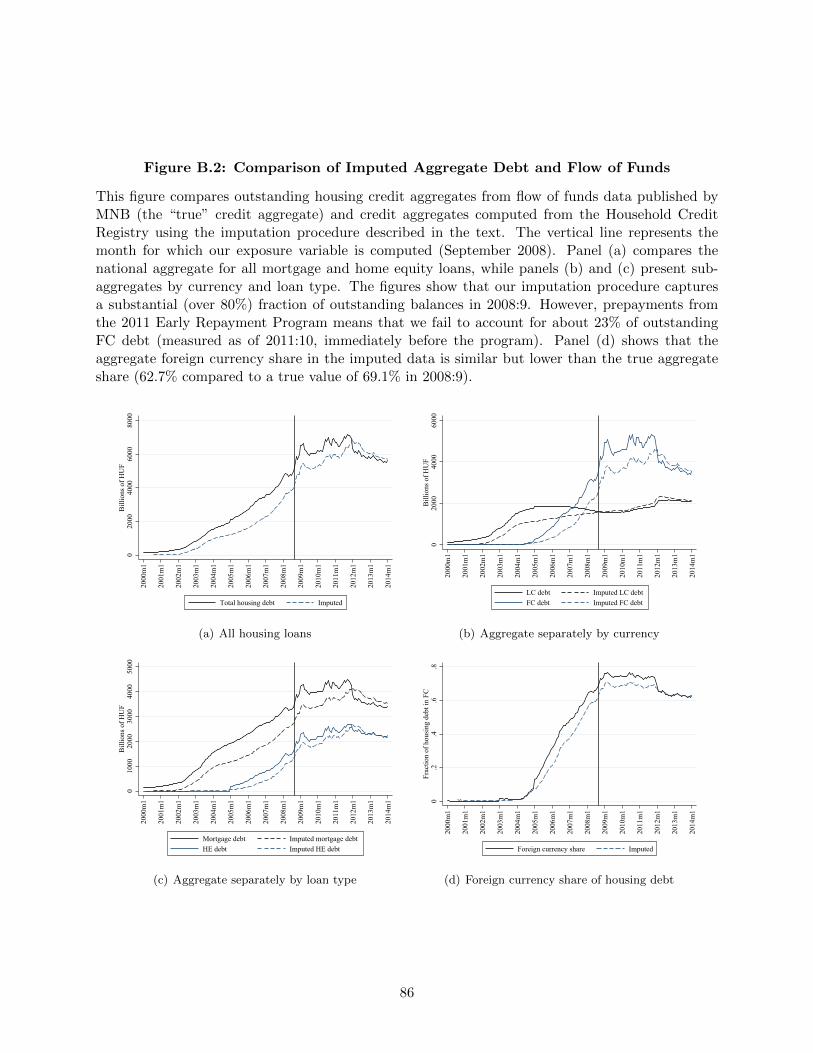
Figure B.2: Comparison of Imputed Aggregate Debt and Flow of Funds

This figure compares outstanding housing credit aggregates from flow of funds data published byMNB (the “true” credit aggregate) and credit aggregates computed from the Household CreditRegistry using the imputation procedure described in the text. The vertical line represents themonth for which our exposure variable is computed (September 2008). Panel (a) compares thenational aggregate for all mortgage and home equity loans, while panels (b) and (c) present sub-aggregates by currency and loan type. The figures show that our imputation procedure capturesa substantial (over 80%) fraction of outstanding balances in 2008:9. However, prepayments fromthe 2011 Early Repayment Program means that we fail to account for about 23% of outstandingFC debt (measured as of 2011:10, immediately before the program). Panel (d) shows that theaggregate foreign currency share in the imputed data is similar but lower than the true aggregateshare (62.7% compared to a true value of 69.1% in 2008:9).

020

0040

0060

0080

00B

illio

ns o

f HU

F

2000

m1

2001

m1

2002

m1

2003

m1

2004

m1

2005

m1

2006

m1

2007

m1

2008

m1

2009

m1

2010

m1

2011

m1

2012

m1

2013

m1

2014

m1

Total housing debt Imputed

(a) All housing loans

020

0040

0060

00B

illio

ns o

f HU

F

2000

m1

2001

m1

2002

m1

2003

m1

2004

m1

2005

m1

2006

m1

2007

m1

2008

m1

2009

m1

2010

m1

2011

m1

2012

m1

2013

m1

2014

m1

LC debt Imputed LC debtFC debt Imputed FC debt

(b) Aggregate separately by currency

010

0020

0030

0040

0050

00B

illio

ns o

f HU

F

2000

m1

2001

m1

2002

m1

2003

m1

2004

m1

2005

m1

2006

m1

2007

m1

2008

m1

2009

m1

2010

m1

2011

m1

2012

m1

2013

m1

2014

m1

Mortgage debt Imputed mortgage debtHE debt Imputed HE debt

(c) Aggregate separately by loan type

0.2

.4.6

.8Fr

actio

n of

hou

sing

deb

t in

FC

2000

m1

2001

m1

2002

m1

2003

m1

2004

m1

2005

m1

2006

m1

2007

m1

2008

m1

2009

m1

2010

m1

2011

m1

2012

m1

2013

m1

2014

m1

Foreign currency share Imputed

(d) Foreign currency share of housing debt

86

Figure B.3: Early Repayment Program Adjustment and Aggregate FC Debt

020

0040

0060

00B

illio

ns o

f HU

F

2004

m1

2005

m1

2006

m1

2007

m1

2008

m1

2009

m1

2010

m1

2011

m1

2012

m1

2013

m1

2014

m1

Flow of funds FC housing debt Credit registry (CR)CR, ERP adjustment #1 CR, ERP adjustment #2

Figure B.4: Method #1 Predicted and Actual 2011 Early Repayment Program DebtReduction by Bank

otp

budapest

erste

raif

unicredit

mkb

cib

k&h

rest of banks

saving coop

45-degree line050

100

150

200

Pred

icte

d w

ith m

etho

d #1

(bn

HU

F)

0 50 100 150 200Debt prepaid in Early Repayment Program (bn HUF)

45-degree line

Notes: This figure plots the amount of debt prepaid through the 2011 Early Repayment Programfor the 8 major banks, the savings cooperatives, and the rest of the banks agains the predictedamount using Method #1.

Figure B.5: Original and ERP Adjusted FC Debt Shares

This figure plots binned bivariate means (binscatter) of the foreign currency debt share adjustedfor the Early Repayment Program against the original FC share (sFCz08).

45-degree line.4.5

.6.7

.8.9

FC d

ebt s

hare

, ER

P ad

just

men

t #1

and

#2

.4 .5 .6 .7 .8 .9FC debt share

ERP adjustment #1 ERP adjustment #2

87

Table B.3: Robustness of Main Results to Missing Data Adjustments

Panel A: Default Rate Change, 2008-10(1) (2) (3) (4)

HH FC debt share, ERP adj. #1 6.69∗∗ 6.23∗∗

(1.07) (0.88)

HH FC debt share, ERP adj. #2 7.19∗∗ 7.81∗∗

(1.05) (0.87)

Full Settlement Controls Yes YesR2 0.039 0.17 0.041 0.19Observations 3108 2678 3108 2678

Panel B: Durable Spending Growth, 2008-10(1) (2) (3) (4)

HH FC debt share, ERP adj. #1 -74.5∗∗ -56.9∗∗

(18.6) (16.8)

HH FC debt share, ERP adj. #2 -66.2∗∗ -74.8∗∗

(21.7) (16.7)

Full Settlement Controls Yes YesR2 0.017 0.27 0.013 0.27Observations 3124 2679 3124 2679

Panel C: Non-Durable Spending Growth, 2008-10(1) (2) (3) (4)

HH FC debt share, ERP adj. #1 -13.8∗∗ -9.70∗

(4.23) (3.87)

HH FC debt share, ERP adj. #2 -11.9∗∗ -9.94∗

(4.34) (3.89)

Full Settlement Controls Yes YesR2 0.019 0.19 0.013 0.19Observations 3124 2679 3124 2679

Panel D: Unemployment Rate Increase, 2008-10(1) (2) (3) (4)

HH FC debt share, ERP adj. #1 1.51∗ 2.22∗∗

(0.61) (0.69)

HH FC debt share, ERP adj. #2 2.52∗∗ 2.68∗∗

(0.69) (0.72)

Full Settlement Controls Yes YesR2 0.0067 0.053 0.017 0.059Observations 3124 2679 3124 2679

Panel E: House Price Growth, 2008-10(1) (2) (3) (4)

HH FC debt share, ERP adj. #1 -32.7∗∗ -25.5∗∗

(6.91) (7.55)

HH FC debt share, ERP adj. #2 -25.3∗∗ -24.3∗∗

(7.78) (7.44)

Full Settlement Controls Yes YesR2 0.024 0.096 0.013 0.095Observations 1932 1856 1932 1856

Standard errors in parentheses clustered at the subregion level.

+,*,** indicate significance at the 0.1, 0.05, and 0.01 levels, respectively.

88

B.2 Wage Estimates from the Structure of Earnings Survey

The Structure of Earnings Survey (SES) is conducted annually by the National Employment Serviceand samples 6% of Hungarian employees, recording information on their income in May. Firmswith 5-20 employees are randomly sampled from the census of enterprises and report informationon all employees. All large firms with at least 20 employees are required to report information ona 10% random sample of employees based on employee date of birth. See Harasztosi and Lindner(2017) for a detailed description of the SES.

We estimate composition adjusted wages at the settlement level in the following manner. Ineach year we run the following regression separately for men and women

ln(Wit) = αt +XitΓt + νit,

where Wit is worker i’s nominal hourly wage (total wage compensation divided by total hours), Xit

is a vector of five-year age dummies (with 41-45 as the omitted category) and education dummies(with high school as the omitted category). We then exponentiate the residual plus the constantto obtain the composition adjusted wage, Wit = eνit+αt and compute the average of Wit in eachsettlement. This procedure yields estimated wage series for about one-third of the settlements inour sample that cover about 82% of the population. With reported hours we also compute theaverage monthly hours in a settlement, conditional on employment.

C Debt Revalaution in an Open Economy Model

C.1 Model Set-Up

We model a region as an island small open economy in a continuum of economies i ∈ [0, 1] followingGalı and Monacelli (2005). To provide simple analytical results, we employ the recent continuoustime formulation of Farhi and Werning (2017). We focus on an unanticipated exchange rate shockat time t = 0, which generates perfect foresight response from the initial steady state.Households. Household preferences are given by

∫ ∞0

e−ρt

[C1−σt

1− σ− N1+ϕ

t

1 + ϕ

]dt,

where consumption is an aggregate of home and foreign goods

Ct =

[(1− α)

1ηC

η−1η

H,t + α1ηC

η−1η

F,t

] ηη−1

.

Home goods are an aggregate of a continuum of varieties with elasticity of substitution ε

CH,t =

(∫ 1

0CH,t(j)

ε−1ε dj

) εε−1

.

89

The parameter α indexes the degree of home bias in consumption. The foreign good is an aggregateof goods from each country with elasticity of substitution γ. In turn, the consumption goodproduced by country i is an aggregate of varieties produced within i:

CF,t =

(∫ 1

0Cγ−1γ

i,t di

) γγ−1

, Ci,t =

(∫ 1

0Ci,t(j)

ε−1ε dj

) εε−1

.

Below we simplify and focus on the case where σ = η = γ = 1 (known as the Cole-Obstfeld case),but we keep the notation general for now.

We follow Farhi and Werning (2017) and assume incomplete markets.56 Specifically, to beconsistent with our empirical setting, the household has access to risk-free debt denominated indomestic and foreign currency. The budget constraint is

EtD∗t + Dt = Eti∗tD∗t + itDt + PtCt −WtNt − Tt −Πt, t ≥ 0,

where Dt and D∗t are debt denominated in domestic and effective foreign currency, and it and i∗tare the home and foreign nominal interest rate.57 In the initial steady state we have E = 1 andi = i∗ = ρ.

Household optimality implies the following first order conditions for logged variables:

σct + ϕnt = wt − pt

ct = σ−1(it − πt − ρ)

ct = σ−1(i∗t − πt − ρ+ e).

Firms. The production function of the firm producing variety j in the home country is Yt(j) =AHNt(j). Real marginal cost in terms of domestic prices is given by MCt = 1+τ

AHWtPH,t

, where τ is a

employment subsidy that is set to offset the monopoly distortion. Log real marginal cost is thus

mct = −ν + wt − pH,t − aH , ν ≡ − ln(1 + τ). (12)

Firms set prices in producer currency in a staggered fashion and can reset prices with arrival rateρδ.Terms of Trade and Real Exchange Rate. It is useful to define and relate the terms oftrade to the various price indexes in the economy. The consumer price index in the home country

is Pt =[(1− α)P 1−η

H,t + αP 1−ηF,t

] 11−η

, where the home producer price index is the standard Dixit-

Stiglitz aggregate over varieties j: PH,t =(∫ 1

0 PH,t(j)1−εdj

) 11−ε

. Define the effective terms of trade

56Galı and Monacelli (2005) focus on the symmetric complete markets case, which simplifies the analysis by removingnet foreign assets as a state variable.

57There is a continuum of symmetric foreign countries. The foreign currency bond is denominated in the effective

spot exchange rate E =(∫ 1

0E1−γi di

) 11−γ

.

90

as the price of foreign goods relative to the price of home goods, St =PF,tPH,t

, and the effective real

exchange rate as Qt =EtP ∗tPt

=PF,tPt

, given producer currency pricing.Home CPI can be log-linearized as

pt = (1− α)pH,t + αpF,t = pH,t + αst ⇒ πt = πH,t + αst. (13)

This allows us to relate the log terms of trade to the log real exchange rate

qt = (1− α)st.

Consumption Risk Sharing and Wealth Effects. We assume all foreign countries are sym-metric. The Euler equation for the home country and country i imply an international risk sharingcondition:

Ct = ΘiCitQ1σi,t.

Taking logs and integrating over i gives us

ct = θ + c∗t +1

σqt,

where θ = θi =∫ 1

0 θidi and c∗t ≡

∫ 10 c

itdi. θ is a term that depends on net foreign debt, and a debt

revaluation that increases the home country’s net foreign debt lowers θ.Goods Market Clearing. Using the standard CES demand functions, the market clearing con-dition for variety j is

Yt(j) = CH,t(j) +

∫ 1

0CiH,t(j)di

= (1− α)

(PH,t(j)

PH,t

)−ε(PH,tPt

)−ηCt + α

∫ 1

0

(PH,t(j)

PH,t

)−ε( PH,tEi,tP iF,t

)−γ (P iF,tP it

)−ηCitdi

Inserting this into the domestic output aggregator Yt =(∫ 1

0 Yt(j)ε−1ε dj

) εε−1

, we have

Yt = (1− α)

(PH,tPt

)−ηCt + α

∫ 1

0

(PH,tEi,tP iF,t

)−γ (P iF,tP it

)−ηCitdi

=

(PH,tPt

)−η [(1− α)Ct + αCt

∫ 1

0

(P iF,tEi,tPH,t

)γ−ηQη− 1

σi,t Θ−1

i di

].

91

Under the assumption that σ = γ = η = 1 the goods market clearing condition simplifies to

Yt = CtSαt

[(1− α) + αΘ−1

], (14)

which can be log-linearized as

yt = ct + αst − αθ. (15)

Using the risk sharing condition ct = θ + c∗t + qt and the fact that qt = (1− α)st yields

yt = c∗t + st + (1− α)θ. (16)

An increase in θ increases demand for home output by (1− α), the share on home goods.

Net Exports. Define net exports in terms of domestic output as nxt =(

1Y

) (Yt − Pt

PH,tCt

). Log-

linearizing and using that Sα = Pt/PH,t yields

nxt = yt − ct − αst = −αθ,

where the last equality uses (15) and hence the assumption of unitary elasticities of substitution.Therefore, when θ > 0 (Θ > 1) the home country can run trade deficits of αθ in each period. Theassumption of unit elasticities simplifies the analysis because it implies that the trade balance isconstant.IS Equation. Differentiating the market clearing condition (15) with respect to time under theassumption of unitary elasticities, we have

yt = ct + αst

Substituting out consumption from the Euler equation, ct = it − πt − ρ, implies

yt = it − πt − ρ+ αs.

Finally, using (13), the dynamic IS equation is

yt = it − πH,t − ρ.

Marginal Cost, Output, and Phillips Curve. To a first order approximation, we can relate

92

domestic output to domestic productivity and employment as

yt = aH + nt.

Using this and other relations, we can rewrite real marginal cost in (12) as

mct = −ν + (wt − pt) + (pt − pH,t)− aH (17)

= −ν + (1 + ϕ)yt + αθ − (1 + ϕ)aH (18)

where we assume σ = γ = η = 1.

The natural level of output that obtains under flexible prices when mc = −µ = ln(

εε−1

), is

thus

ynt = aH +ν − µ1 + ϕ

− αθ

1 + ϕ. (19)

The deviation from real marginal cost relative to the initial natural level (with θ = 0) is

mct = (1 + ϕ)yt + αθ. (20)

Calvo price setting implies that domestic inflation dynamics are given by the New-KeynesianPhillips curve

πH,t = ρπH, − λmct, λ = ρδ(ρ+ ρδ) (21)

which, using (20), can be rewritten as

πH,t = ρπH, − κyt − λαθ, κ = λ(1 + ϕ). (22)

Initial Flexible Price Steady State. In the initial steady state θ = 0. Moreover, we assumeaH = c∗ = 0. From (16) and (19), the natural level of output and terms of trade are simplyyn = 0, sn = 0.

C.2 Consequences of a Household Debt Revaluation

As discussed in section 3.1, we assume that in the initial steady state the nominal exchange rateequals one, E = 1. The household is long in domestic currency assets and borrows in foreigncurrency, so debt in terms of output satisfies D∗+ D = 0, D∗ > 0.58 The economy is in the natural

58The assumption that D∗+D = 0 is without loss of generality, as we can always redefine the initial natural allocationas one with a different wedge in the consumption risk sharing condition.

93

allocation with θ = 0 and balanced trade.At time zero there is ∆e% depreciation that raises debt to ∆eD∗ > 0. This is the fundamental

shock we study. The increase in debt implies that the economy must run trade surpluses. Under theassumption of unit elasticities of substitution, the trade balance is constant and equals nx = −αθ.The country budget constraint therefore implies that net foreign debt relative to initial output is

∆eD∗ =∫∞

0 e−∫ t0 isdsnxdt =

∫∞0 e−ρtnxdt = nx

ρ . As a result, the debt revaluation implies that thewedge in the risk sharing condition declines by

θ = −ρ∆eD∗

α.

This term has the intuitive property that the increase in debt is smoothed according the rate atwhich the households can borrow ρ.

How does the exchange rate shock and associated debt revaluation affect output and prices?We can trace the effect by solving the following system:

πH,t = ρπH,t − κyt + λρ∆eD∗ (23)

yt = it − πH,t − ρ (24)

y0 = −1− αα

ρ∆eD∗ + ∆e. (25)

Equation (23) is the standard New-Keynesian Phillips curve, adjusted for the wealth effect of thedebt revaluation. Equation (24) is the dynamic IS curve. Given that we think of the home economyas an independent region within a currency union, we assume that it = ρ, so that domestic monetarypolicy does not react to the shock. Equation (25) is the initial goods market clearing condition.The nominal exchange rate enters the initial condition, as it jumps by ∆e, depreciating the termsof trade, but prices are sticky and hence evolve smoothly.59

Analytical Solution. We can write the system in (23)-(24) as Xt = AXt + Bt and apply thetransformation Zt = V −1Xt, where V −1AV = D. Here V is the matrix of eigenvectors of A, andD is the diagonal matrix of eigenvalues of A:

A =

ρ −κ

−1 0

, D =

ν 0

0 ν

, V =

−ν −ν

1 1

, ν =ρ+

√ρ2 + 4κ

2, ν =

ρ−√ρ2 + 4κ

2

59Empirically, the terms of trade moves significantly less than one for one with exchange rate shock (Boz et al.(2017)). A weaker quantitative effect of the exchange rate channel through expenditure switching strengthens ouridentifying assumption, as it implies that the expenditure switching channel will also matter less for output in thecross-section of regions.

94

The system we want to solve is then Z = DZ + V −1B, or

z1 = νz1 +λρ∆eD∗

ν − ν(26)

z2 = νz2 +λρ∆eD∗

ν − ν(27)

(28)

The general solution is

z1t = b1eνt − λρ∆eD∗

ν − ν1

ν(29)

z2t = b2eνt − λρ∆eD∗

ν − ν1

ν, (30)

where b1 and b2 are constants. We set b1 = 0 for the saddle path stable solution. Using Xt = V Zt,we can obtain the solution in terms of the original variables

Xt =

−νeνtb2

b2eνt − λρ∆eD∗

ν−ν(

1ν −

1ν

) (31)

To obtain b2, we use the initial condition (25)

b2 = −1− αα

ρ∆eD∗ + ∆e+λρ∆eD∗

ν − ν

(1

ν− 1

ν

)

The output response to the exchange rate shock is then of the form provided in the main text (1)

yt =

(−1− α

αeνt − (1− eνt) λ

ν − ν

(1

ν− 1

ν

))ρ∆eD∗ + ∆e · eνt

yt =

(−1− α

αeνt + (1− eνt) 1

1 + ϕ

)ρ∆eD∗ + ∆e · eνt

yt = βt∆eD∗ + γt∆e (32)

and the response of domestic inflation is

πH,t = −νeνt(−1− α

αρD∗∆e− ρ∆eD∗

1 + ϕ+ ∆e

).

The debt revaluation channel tends to lower inflation and depreciate the terms of trade, as demandfalls and labor supply expands.

95