Horrible Trade-offs in a Pandemic: Lockdowns, Transfers, Fiscal Space, and Compliance

Ricardo Hausmann, Ulrich Schetter

CID Faculty Working Paper No. 382 July 2020

© Copyright 2020 Hausmann, Ricardo; Schetter, Ulrich; and the President and Fellows of Harvard College

at Harvard University Center for International Development

Working Papers

Horrible Trade-offs in a Pandemic: Lockdowns,Transfers, Fiscal Space, and Compliance∗

Ricardo Hausmann

Harvard Kennedy School

and Santa Fe Institute

Cambridge, MA 02138

ricardo hausmann@hks.harvard.edu

Ulrich Schetter

Harvard Kennedy School

Cambridge, MA 02138

ulrich schetter@hks.harvard.edu

First Version: April 2020This Version: July 2020

Abstract

In this paper, we develop a heterogeneous agent general equilibrium framework to ana-lyze optimal joint policies of a lockdown and transfer payments in times of a pandemic.In our model, the effectiveness of a lockdown in mitigating the pandemic depends on en-dogenous compliance. A more stringent lockdown deepens the recession which impliesthat poorer parts of society find it harder to subsist. This reduces their compliance withthe lockdown, and may cause deprivation of the very poor, giving rise to an excruciat-ing trade-off between saving lives from the pandemic and from deprivation. Lump-sumtransfers help mitigate this trade-off. We identify and discuss key trade-offs involvedand provide comparative statics for optimal policy. We show that, ceteris paribus, theoptimal lockdown is stricter for more severe pandemics and in richer countries. We thenconsider a government borrowing constraint and show that limited fiscal space lowersthe optimal lockdown and welfare, and increases the aggregate death burden during thepandemic. We finally discuss distributional consequences and the political economy offighting a pandemic.

Keywords: COVID-19, lockdown, fiscal policy, government borrowing constraint, po-litical economy, inequality, developing countries

JEL: E62, F4, H12, I14, I18

∗We would like to thank Eduardo Fernandez Arias, Andres Gomez, Frank Neffke, Maik Schneider, FedericoSturzenegger, Mariano Tommasi, Rodrigo Wagner, and seminar participants at the Harvard Growth Lab andthe Universidad de San Andres for valuable comments and suggestions.

1 Introduction

COVID-19 is the most severe global pandemic since the Spanish flu of 1918/1919, and it

threatens millions of lives. To fight the pandemic and to limit its death burden, governments

all over the world impose drastic measures. For lack of more targeted policies, they opt for

partial and full lockdowns that bring significant parts of the economy to a halt. The economic

consequences are dramatic with unemployment rising and GDP falling at unprecedented

rates. A surging economic literature suggests that the enormous value at stake in terms

of the pandemic may justify such drastic measures, even if they result in income losses in

the order of 10, 20, 30% of GDP or higher.1 Yet, these shocks need to be absorbed at the

individual and at the country level, and some countries may be less able to do so than others.

To cushion the economic shocks, central banks in industrialized countries loosen monetary

policy and governments announce enormous fiscal stimuli, financed via public debt. As of

May 2020, total announced fiscal measures amount to more than 10% of GDP in countries

like the US, South Korea, Switzerland, or Australia, for example.2 Similar measures may not

be feasible in large parts of the developing world. Many developing countries had limited

fiscal space to begin with, only to see it collapse as a consequence of the global impact

of COVID-19 on commodity prices, tourism, remittances, and capital flows (Hausmann,

2020; Hevia and Neumeyer, 2020). These global shocks are by themselves a major hit to the

economy, increasing the need for supportive policies even further. While such policy measures

are important in industrialized countries, they would be even more valuable in developing

countries where a larger fraction of the population is in poverty. Hunger is projected to

almost double in the wave of the COVID-19 pandemic (World Food Programme (WFP),

2020).

What does this imply for policy? How does the optimal lockdown depend on accompanying

policy measures to alleviate the economic shock? How do such measures impact compliance

with a lockdown and welfare? What are the cost of limited fiscal space in a pandemic and how

does it affect policy? What if parts of the population are at or close to subsistence, already

struggling with surviving the recession caused by the global shock? Are lockdowns a luxury

good that is desirable only for countries rich enough to be able to bear the consequences?

In this paper, we provide first answers to these questions by presenting a tractable economic

model that allows to jointly analyze optimal lockdowns and lump-sum transfers. Our main

1See e.g. Acemoglu et al. (2020); Eichenbaum et al. (2020a); Farboodi et al. (2020); Hall et al. (2020).2Source: https://projects.iq.harvard.edu/covidpt/global-policy-tracker, accessed on 5/8/2020. When in-

cluding loans, equity injections, and guarantees, the total volume of fiscal stimuli even exceeds 30% of GDPin the case of Germany and Italy (International Monetary Fund (IMF), 2020a).

1

focus is on developing countries, but the mechanisms we analyze matter more generally in

countries where parts of society suffer from deprivation or are threatened to ’die of despair’

(Case and Deaton, 2020). We outline our model in Section 2: There are two periods, the

present and the future, the latter can be interpreted as an infinite horizon steady state. Also,

there is a continuum of households that differ in their ability. Households inelastically supply

1 unit of labor and derive utility from consumption of a final good that is produced with

constant returns to scale using efficiency units of labor as the only input. To survive, per-

period consumption of a household needs to meet a subsistence level c > 0. In the first period,

the economy is unexpectedly hit by a pandemic. The pandemic causes deaths from the disease

and a temporary loss in TFP—the latter can also be attributed to global economic shocks

due to the global nature of the pandemic. The government can decide to fight the pandemic

via a lockdown, which requires households to reduce their labor supply, and impacts TFP via

e.g. distorted value chains, but also via a better control of the pandemic. In line with the idea

that the trade-off between economic loss and loss of life need not be negative everywhere (see

e.g. Acemoglu et al. 2020, Figure 1), we allow the TFP effect of a lockdown to be positive

for small values of the lockdown. Eventually, however, it will be distortive, and aggregate

TFP declines. The government can accompany the lockdown with transfer payments to be

financed via international borrowing at a fixed rate, but subject to a borrowing constraint.

Households comply with the lockdown as long as it allows subsistence.

In Section 3, we show that the lockdown and transfer payments have intricate effects on the

economy. On the one hand, the lockdown reduces social interactions and thus mitigates the

pandemic and its death burden. On the other hand, it deepens the recession, which lowers

compliance with the lockdown and may imply that poorer parts of the population suffer

from deprivation and are no longer able to subsist. Transfer payments can help these parts of

the population through the recession and, more generally, allow for consumption smoothing

between the present and the future. They also increase compliance with the lockdown and

thus have an indirect beneficial effect on the pandemic. On the other hand, they lower future

utility, and more so, the smaller the future population to service the debt.

These heterogeneous and interdependent effects notwithstanding, our set-up is tractable

enough to analytically characterize optimal policy. We show that optimal policy always

involves a trade-off between ’lives and livelihoods’, i.e. between economic losses and loss of

life. As excruciating as this trade-off may be, in developing countries a lockdown may involve

an even more horrible trade-off: One between saving households from the pandemic or saving

them from dying from deprivation. We show that the optimal lockdown always fights the

pandemic at the margin, but this fight against the pandemic might imply deprivation of the

poorest households, particularly in societies where part of the population is close to subsis-

2

tence and if the future weighs large compared to the present. This being said, we provide

numerical illustrations that consistently suggest that with optimal transfers in place—i.e. in

an unconstrained optimum—a very small or even zero fraction of the population is threatened

to die from deprivation. In other words, in the absence of borrowing constraints, subsistence

of the poorer parts of society imposes limits on the optimal fight against a pandemic. Indeed,

we show analytically that the optimal lockdown is more stringent for richer countries, i.e.

poorer countries are more heavily concerned by deprivation vis-a-vis the pandemic. In that

sense, a lockdown may be seen as a ’luxury good’. Importantly, lump-sum transfers help

alleviate this trade-off, and we show that at the margin these policy tools are complements,

i.e. ceteris paribus larger transfers rationalize a more stringent lockdown.

We next consider borrowing constraints, which have a major effect on optimal policy, deaths,

and welfare. In particular, the complementarity between the lockdown and lump-sum trans-

fers implies that—when confronted with a borrowing constraint—it is optimal to fight less

the pandemic. Intuitively, if part of the population is close to subsistence and the government

does not have the fiscal space to support the poor, fighting a pandemic via a lockdown that

deepens the recession is very costly. As a consequence, the aggregate death burden is higher,

welfare lower, and if the borrowing limit is small, it may no longer be true that the govern-

ment can save the vast majority of its population from dying from deprivation, highlighting

the dire need of developing countries to receive financial support in times of a pandemic.

We illustrate these effects and their impact on optimal policy by means of a numerical

example in Section 4. This example delivers additional insights on the effects of borrowing

constraints: It suggests that optimal transfers as a share of steady state GDP are lower

in richer countries. Accordingly, the gap between constrained and unconstrained optimal

policies is larger for poorer countries, i.e. borrowing constraints are particularly costly for

the most vulnerable societies. It further shows that the distance between constrained and

unconstrained optimal policies is larger, the more severe the disease.

The pandemic and the optimal policy response have important distributional consequences.

On the one hand, the lockdown benefits the least—and may even hurt—the poorest house-

holds in a society. These households may not be able to afford full compliance with the

lockdown and, hence, face a higher probability of dying from the disease. In the extreme,

they may even not be able to live through the recession and die from deprivation. On the

other hand, for the same reasons, these households are the ones that benefit the most from

lump-sum transfers. We discuss these distributional consequences and the implied political

economy of fighting a pandemic in Section 5, where we derive a single-crossing result for

individual preferences over policies and discuss its implications. In this section, we also show

3

that supporting vulnerable parts of society in times of a pandemic is in the self-interest of

the rich if the externality of working on the pandemic is sufficiently large and the future suf-

ficiently important vis-a-vis the present. We further discuss robustness of our main findings

to changes in our simplifying assumptions.

Finally, Section 6 concludes.

Relation to literature

Our paper contributes to the rapidly growing literature that uses economic models to analyze

the COVID-19 pandemic and policy options. A series of recent papers build on the so called

SI(E)R model (Kermack et al., 1927) or variants thereof to analyze the evolution of the

pandemic and optimal containment policy. Atkeson (2020), Bodenstein et al. (2020), and

Rampini (2020) perform policy experiments. Acemoglu et al. (2020), Alvarez et al. (2020),

and Piguillem and Shi (2020) solve planning problems that trade off the economic losses

from a lockdown and the death burden of the disease. Eichenbaum et al. (2020a), Farboodi

et al. (2020), Garibaldi et al. (2020), Jones et al. (2020), Krueger et al. (2020) endogenize

agents’ responses to the pandemic and emphasize externalities in the presence of a pandemic

that relate to the transmission of the disease and the congestion in the healthcare system.3

von Carnap et al. (2020) apply the Eichenbaum et al. (2020a) model to show that—due to

lower income and differences in the demographic structure—optimal lockdowns are much

smaller in developing countries when compared to the US.4 None of these papers consider

(complementary) policy tools and how they affect optimal lockdowns and key trade-offs

involved.5 Baqaee and Farhi (2020), Bigio et al. (2020), Caballero and Simsek (2020), Faria-

e-Castro (2020), and Cespedes et al. (2020) on the other hand, study macroeconomic shocks

during the COVID-19 pandemic and policy options to counteract these, but do not consider

policies to fight the pandemic itself. Moreover, with the exception of Cespedes et al. (2020),

these papers do not consider borrowing constraints.6

By contrast, we analyze optimal joint policies of lockdown and lump-sum transfers in set-ups

with and without borrowing constraints. In that sense, our paper is closest to Guerrieri

3Eichenbaum et al. (2020b) analyze smart containment policies that involve intense testing and quaran-tining infected people to find that—if feasible—it is drastically more efficient than general lockdowns.

4von Carnap et al. (2020) also introduce a subsistence consumption level, which will play an important rolein our analysis, but they consider representative agents and, hence, consumption is always above subsistence.

5Eichenbaum et al. (2020a) model containment measures as a tax on consumption whose revenues arerebated as lump-sum transfers. This tax, however, cannot be optimized independently from the lockdown.

6Cespedes et al. (2020) consider private borrowing constraints that may bind in times of a pandemic dueto the endogenous value of collateral. They argue that by relaxing liquidity constraints, governments canfocus the economy on the good equilibrium. This, however, requires ample fiscal space, i.e. they provide achannel for need of fiscal space in times of a pandemic that is complementary to the one we consider.

4

et al. (2020), Glover et al. (2020), and Alon et al. (2020). Guerrieri et al. (2020) present

a theory of sector-specific ’Keynesian supply shocks’, i.e. negative supply shocks that have

negative demand spillovers to other sectors, in a two-sector model with nominal rigidities.

Most relevant for our purposes, they also consider an extension where the sector-specific

supply shock is explicitly modeled as a lockdown in response to a pandemic. They pro-

vide a sufficient condition for first-best efficiency of a complete lockdown of one sector in

combination with stabilizing monetary policy intervention plus social insurance in case of

a borrowing constraint for households. Glover et al. (2020) introduce heterogeneous agents

into a macro-epidemiological model with two-sectors and costly transfers between working

and non-working parts of the population, where households may not work due to age, health

status, or a government-imposed closure of their sector. They use a calibrated version of their

model to highlight distributional conflicts of lockdown policies and, quite intuitively, show

that the optimal lockdown of the ’luxury goods’ sector is smaller the costlier is redistribution.

Our work differs along several dimensions: We consider international borrowing that allows

for intertemporal consumption smoothing. More importantly, we allow for feedback effects

from Macro-policies—debt-financed lump-sum transfers in our case—on the pandemic and

the effectiveness of a lockdown in fighting the pandemic. Specifically, we consider an econ-

omy with a continuum of heterogeneous agents and analyze how lump-sum transfers affect

compliance with a lock-down, the ability of households to live through the recession, and,

hence, the optimal lockdown. Notably, this focus on countries where parts of society may

suffer from deprivation also distinguishes our work from most of the aforementioned list of

papers.

Alon et al. (2020) build on Glover et al. (2020) to perform a preliminary quantitative account

of optimal policy in a developing country set-up with an informal sector. Lockdowns are

effective only in the formal sector and households can choose in which sector to work. The

government can support households via costly transfers, financed via taxes and emergency

bonds. According to their analysis, welfare losses from the pandemic are smaller and optimal

lockdowns tend to be less strict in developing countries. We complement their work along

several dimensions. Most importantly, we introduce a subsistence consumption level and show

how this may give rise to much larger welfare losses in the developing world, in particular if

government borrowing is constrained. Moreover, we present a tractable model, which allows

us to analytically identify and discuss main effects and, hence, to analyze key trade-offs in a

transparent way and to derive robust comparative statics.

Chang and Velasco (2020) discuss feedback effects from economic policy on the pandemic in

a stylized set-up that is different from ours along important dimensions. In their model, a

subset of the population has been tested for the disease, and those who have been found to

5

be susceptible then endogenously choose whether or not to work.7 There may be multiple

equilibria where either all or none of these susceptible individuals work. Lockdown and

targeted transfers to unemployed workers may complement each other if it requires a ’big

push’ to shift the economy from a ’bad’ to a ’good’ equilibrium and neither of the policy

measures is sufficient in itself. Our main mechanisms are different and we identify and

discuss various convoluted effects of a lockdown and transfer payments on the pandemic and

welfare. Moreover, we consider the effect of a borrowing constraint on optimal policy and

welfare, and discuss political economy-effects of fighting a pandemic in developing countries.8

Finally, our paper also contributes to the broader economics literatures analyzing infectious

diseases on the one hand (e.g. Bell et al. (2006), Bloom and Canning (2006), Greenwood

et al. (2019)), and causes and consequences of government borrowing constraints on the other

hand (e.g. Stiglitz and Weiss (1981), Bulow and Rogoff (1989), Gavin and Perotti (1997),

Caballero and Krishnamurthy (2001), Kaminsky et al. (2004), Eichengreen et al. (2007),

Chari et al. (2020)).9 We add to these literatures in that we consider optimal joint policies of

containment measures to combat a pandemic and transfer payments to support households

in need, and how they are affected by a government borrowing constraint.

2 Model

2.1 Economic Environment

We consider an economy with a continuum of measure 1 of households who differ in their

ability a. To simplify the exposition, we assume that there are two periods only: In the

first period—the present—, the economy faces a pandemic. The second period—the future—

is a post-pandemic period, which we can think of as a reduced form representation for the

present value of an infinitely repeated post-pandemic steady-state, as further discussed below.

The pandemic imposes two costs on the economy: It causes a fraction of the population to

7Agents who get tested positive are compelled to stay home. The decision to work of the susceptibletherefore entails a positive externality as they are healthier than the average. Similarly, Eichenbaum et al.(2020b) argue that testing, if not combined with strict containment of infected, has a negative externalitybecause a positive test increases the incentives to work for selfish agents.

8See e.g. Gourinchas (2020) and Loayza and Pennings (2020) for informal discussions of emerging policyissues in the COVID-19 pandemic, the latter with a focus on developing countries. Loayza (2020) discussespolicy options to fight the pandemic in developing countries where poverty is rising and fiscal space is limited.Ray et al. (2020) consider the case of India and discuss horrible trade-offs in times of a pandemic in developingcountries.

9While our focus is on a borrowing constraint, at a more general level we consider (short-run) constraintson the government to mobilize resources. In that sense our work is also, but less closely, related to theliterature analyzing causes and consequences of limited fiscal capability, e.g. Aizenman et al. (2007), Besleyand Persson (2009), and Gersbach et al. (2019).

6

die from the disease and involves a total factor productivity (TFP) loss during the time

of the pandemic. Depending on the development stage of the economy, this recession may

cause an additional death-toll if part of the population is at or close to subsistence. The

government can decide to fight the pandemic by imposing a lockdown θ. The lockdown,

however, deepens the recession as it decreases aggregate labor supply and has a negative effect

on TFP. Households comply with the lockdown only if it allows subsistence. To lessen the

burden of the recession, the government can cushion the lockdown with lump-sum transfers

T which have to be financed via borrowing, subject to a borrowing constraint. In the second

period, the government levies a lump-sum tax to finance its debt-payments.

2.1.1 Households

Households differ in their ability a which is distributed according to some atomless distri-

bution with CDF F (a) and support A. In what follows, we will use f(a) to denote the

associated PDF, and identify households by their ability. Households inelastically supply 1

unit of labor. During the pandemic, the government can impose a lockdown θ and force its

citizens to lower their labor supply. We assume that households comply with this lockdown

up to the point where compliance would imply deprivation as further detailed below, and use

l(a) to denote the period-1 labor supply of household a.

Households receive instantaneous utility of consumption according to

u(c) = v(c)− c, v(c) := cα, 0 < α ≤ 1,

where c denotes the level of consumption and c denotes the subsistence level.10 If in any

given period c < c the household dies. We assume that this death—and a potential death

caused by the pandemic—occurs at the end of the period.

We choose the consumption good to be the numeraire. There are no private opportunities to

lend or borrow,11 implying that per-period consumption just equals per-period income. Let

w denote the wage rate per efficiency unit of labor. Consumption of household a in period

s ∈ {1, 2} is then given by

c1(a; θ, T ) = w1 · a · l(a) + T (1)

c2(a; τ) = w2 · a− τ,

where T is a lump-sum transfer financed via government borrowing as detailed below, and

τ the lump-sum tax that the government levies in the second period to pay for its debt.

10As an alternative, we could consider Stone-Geary-type preferences, u(c) = (c − c)α. This would notfundamentally change our main insights and we therefore opt for the slightly simpler specification in themain text. We briefly discuss the case of more than one goods in Section 5.1.

11See Section 5.1 for a discussion.

7

Consumption in the second period is conditional on survival. The expected lifetime utility

of household a is then given by[ ]α [( ) ]U(a) = w1 α· a · l(a) + T − c+ π(a) · β · w2 · a− τ − c .

In the above, β is the discount factor which—consistent with our interpretation of period

2 as the present value of an infinitely repeated steady state—we think of as being large,˜

i.e. β = β ˜˜ for some per-period discount factor β close to 1. π(a) is the probability that

1−βhousehold a survives the first period. For most of what follows, we do not need to explicitly

consider the utility of household a, and we therefore postpone the discussion of π(a) to

Section 5.2, where we consider the distributional consequences and political economics of

combating a pandemic.

In what follows, we will not need the time-superscripts s and we therefore omit them through-

out.

2.1.2 Pandemic

The pandemic hits the economy in the first period only.12 Its severity depends on the amount

of interactions between households in the economy, which can be summarized by the aggregate

labor supply L in period 1.13 Accordingly, we summarize the pandemic by a function P (L),

with the following properties:

Assumption 1

P (L) = Lλ, λ > 1

L is equal to 1 in the steady-state, but may be lower during the pandemic as further detailed

below. Hence, P (L) ∈ [0, 1] and we can therefore think of P as summarizing how bad the

pandemic is relative to the case of L = 1. The pandemic is the less severe the more effectively

the government lowers L, and it is convex in L. We will get back to this point shortly.

The pandemic causes a recession as detailed in Section 2.1.4 below. In addition, the pan-

demic has a health burden. As far as pure health expenditures are concerned, these can be

interpreted as being reflected in the TFP effect discussed below as such health expenditures

12That is, we implicitly assume that either recovered households are immune against the disease, in linewith the widespread use of S(E)IR(D) models in the economics literature on COVID-19, such that herd-immunity can be reached by the end of period 1. Or, that a treatment or vaccine is available by the end ofperiod 1. Hence, our set-up is flexible enough to accommodate situations where recovered households are not(permanently) immune.

13Note that there are no private savings in the economy, i.e. L can be seen as not only summarizingsupply-side channels of disease transmission but, up to the lump-sum transfers of the government consideredbelow, demand-side channels as well.

8

lower income available for other forms of consumption. The pandemic, however, also causes

fatalities d(P ), where we assume:

Assumption 2

d(P ) = δ · P, δ > 0

In the above, δ is the death burden of the pandemic with full employment (L = 1). The death

burden is then linear in the size of the pandemic, i.e. we can think of P as being ’normalized’

in terms of its death burden. P (L) can therefore be seen as summarizing various forces:

The effect of a lockdown on the rate of disease transmission, the effect of the rate of disease

transmission on the overall extend of the pandemic and the size of its peak, and the effect of

the latter on the death burden of the pandemic. We argue in Appendix B.1 with reference

to a simple SIR model that the overall relationship between d(P ) and L is plausibly convex,

in line with our assumptions.

2.1.3 Policy instruments

The government can decide to fight the pandemic by imposing a lockdown θ ∈ [0, 1], where

a lockdown of size θ requires households to reduce their labor supply in period 1 from its

steady state level 1 to a level (1− θ). Next to decreasing L, the lockdown lowers TFP, due to

e.g. distorted supply chains as discussed below. The government can cushion the effects of

the pandemic and the imposed lockdown via a lump-sum transfer t which is to be financed

via foreign borrowing and which is expressed as a fraction of (pre-pandemic) steady state

GDP, i.e. the per capita transfers are

T = t · A · µa,∫where here and below we use µa := ∈A a · f(a)da to denote the average ability in the

a

¯economy, and where A denotes steady-state TFP as detailed below. Borrowing is subject to

a constraint b as a percentage of steady-state income, that is

t ≤ b. (2)

Borrowing comes at an interest rate r. Consistent with our interpretation of period 2 as

the present value of an infinitely repeated steady-state, we assume that the foreign debt is

infinitely rolled over,14 with interest payments financed via a lump-sum tax, for simplicity.

The lump-sum transfer—next to smoothing consumption—has the main effect of saving

poorer households from deprivation and increasing compliance with the lockdown. We con-

sider these effects in Section 2.2 and discuss production first.

14If r > β, this may not be optimal. Note, however, that this is not essential as we are imposing norestrictions on r and an optimal pay-back scheme given r would simply lower the effective cost of borrowing.

˜

9

2.1.4 Production

Production is constant returns to scale with respect to its only input efficiency units of labor,

a · l(a), ∫Y = A · a · l(a) · f(a)da,

a∈A

¯where A is a total factor productivity (TFP) term, which is equal to A in the steady state.

TFP is, however, lower in period 1. For one thing, the pandemic causes a recession. For

another, the government-induced lockdown will lower TFP further as it e.g. distorts supply

chains in the economy. Taken together, TFP in the first period is given by

¯A := A · γP · g(θ), (3)

where γP is a baseline effect in period 1 and g(θ) a lockdown-induced TFP effect. γP can be

interpreted as capturing both a direct domestic effect of the pandemic and negative foreign

economic shocks due to the global nature of the pandemic. We make the following assumption

on these effects:

Assumption 3

(i) g(0) > g(1) (ii) g′′(·) < 0 (iii) γP · g(·) < 1

Here and below, we use a superscript ′ (′′) to denote the first (second) derivative of a function.

Note that Assumption 3 does not rule out the possibility that TFP is increasing in θ for θ

close to 0, i.e. g′(0) > 0. We allow for (but do not require) this possibility as a simple way

of introducing a potential positive contemporaneous net effect of a lockdown on the economy

as in e.g. Acemoglu et al. (2020, Figure 1). In either case, TFP is always lower than in

the steady state (Assumption 3(iii)), TFP is concave, reflecting the idea that a lockdown is

increasingly distortionary the stricter it is (Assumption 3(ii)), and TFP is lower with a full

lockdown than with no lockdown (Assumption 3(i)).

Markets are perfectly competitive such that labor earns its marginal product and the wage

per efficiency unit of labor is simply given by

w = A. (4)

¯We assume that A · a ≥ c for all a ∈ A, i.e. that in normal times all households can subsist.

2.2 Labor supply and aggregate deaths for given policy

Due to the pandemic and the lockdown, the economy is in a recession in period 1. As

a consequence, poor households may—given full compliance with the lockdown—see their

10

income fall below the subsistence level. Using Equation (4) in Equation (1), and combining

it with the fact that under full compliance l(·) = (1− θ), we observe that this is the case for

all households with ability a ≤ a2, where

¯c− t · A · µaa2 := . (5)

(1− θ) · A

We assume that the government has the power to fully enforce the lockdown up to subsistence,

that is households a ≤ a2 supply just enough labor to avoid dying from deprivation.15 For

sufficiently poor households, however, and if the recession is deep, the household income falls

below the subsistence level even if they supply 1 unit of labor. This is the case for households

a ≤ a1, where− ¯c t · A · µa

a1 := . (6)A

Taken together, this implies for labor supply in period 1 of household a:(1− θ) if a ≥ a 2

l(a) = · ¯c−t A·µ a ≥ , (7) a· if a2 > a a1A1 otherwise

and for aggregate labor supply in period 1∫ a2 − · ¯c t A · µaL = F (a1) + · f(a)da+ (1− θ) · [1− F (a2)]. (8)

a1a · A

These discussions point to a horrible moral trade-off that policy makers may face in developing

countries: If part of the population is at or close to subsistence and the recession is bad, a

fraction F (a1) of the population may die from deprivation, whether or not they themselves

are infected by the pandemic, implying that the total death burden in period 1 is given by:

D = F (a1) + [1− F (a︸ ︷︷ ︸ ︸ 1)] · δ · P (L) (9)︷︷ ︸economic pandemic

In other words, in developing countries governments may not only be confronted with choosing

between lives and livelihoods, but between lives and lives. The government can use the

lockdown to trade off between these two sources of deaths, and accompany the lockdown

with transfers to alleviate either of them. We discuss these issues and government policy

more generally next.

15There may be sources of imperfect compliance other than a threat of deprivation. Incorporating thesewould reinforce the complementarity between a lockdown and transfers and would increase the need for fiscalspace, but the various effects of the two policy instruments discussed below and our main insights wouldqualitatively be the same.

11

3 Policy

The government chooses the size of the lockdown θ and the lump-sum transfers t to maximize

aggregate welfare of its citizens. As the previous discussions show, poorer households face

a higher probability of dying. We will get back to analyzing the ensuing distributional

consequences of a lockdown and political economy implications in Section 5.2. For now,

we focus on aggregate welfare effects and assume that the government, in its optimization

problem, assigns the same value to each life. In our model, this essentially boils down to

assuming that the ability distribution in the surviving population is the same as in the entire

population, irrespective of who exactly is dying.16 Aggregate welfare is then given by:17∫ [ ]W = v(A · a · l(a) + t · A · µa)− c · f(a)da

a∈A ∫ [ ( ) ]¯t · A · µa−D) · ¯+ (1 β · v A · a− r · − c · f(a)da. (10)a∈A 1−D

The government chooses (θ, t) to maximize (10) subject to θ ∈ [0, 1], (2), and taking into

account the effect of its policy on A, {l(a)}a∈A, P , and D. Using (7), the government decision

problem boils down to∫ ∫[ ] a2

¯max W = v(A · a+ t · A · µa)− c · f(a)da+ [v(c)− c] · f(a)daθ,t a∈A∫ :a≤a1 a[ ] 1

+ v((1− θ) · A · a+ t · A · µa)− c · f(a)daa∈A:a≥a2 ∫ [ ( ) ]

· ¯t A · µa+ (1−D) · ¯β · v A · a− r · − c · f(a)da (11)

a∈A 1−Ds.t. θ ∈ [0, 1]

t ≤ b,

where A, a1, a2, and D are as defined in Equations (3), (5), (6), and (9).

16Alternatively, this may be interpreted as a simple economy where households do not differ in their innateabilities, but in the productivity of their realized jobs, assuming that the distribution of jobs is scale invariant.While we would argue that attaching a lower value to the lives of poorer households is not desirable for thepurpose of an aggregate-welfare analysis, it is nevertheless interesting to note that our main insights wouldqualitatively be the same in such case. The main difference would be that the cost of death from deprivationwould be lower vis-a-vis the cost of death from the pandemic, which are arguably more equally distributedacross the population. As a consequence, it would ceteris paribus be beneficial to fight more the pandemicand spend less on saving poorer parts of society from deprivation.

17Households may not be able to pay the lump-sum tax in future. In such case, the tax burden would needto be higher for richer households. To simplify the exposition, we ignore this possibility, which would notmaterially impact our results and, in particular, would not at all affect our analysis of Section 3.1. We getback to how debt-service costs are financed in Section 5.2, where we consider the distributional consequencesof fighting a pandemic.

12

θ and t have various effects on the economy: They jointly impact consumption today and

tomorrow—and differentially so for households with different abilities—, TFP, aggregate

labor supply, the pandemic, and hence the death burden in period 1. Optimal policy therefore

involves intricate and convoluted trade-offs, and we will study these next. We begin with

considering high-level trade-offs between lives and livelihoods on the one hand, and economic

and pandemic fatalities on the other hand, before zooming in on the details. Throughout, we

will use a superscript ∗ to denote variable values in the social optimum, and θ∗(t) to denote

the optimal lockdown for given transfers, i.e. θ∗(t∗) = θ∗.

In light of the COVID-19 pandemic, it is debated whether or not fighting the pandemic

involves a trade-off between saving lives and livelihoods. In our model, we allow for the

possibility that fighting the pandemic may have a positive effect on the economy by not

ruling out that g′(0) > 0, i.e. that fighting the pandemic initially has a positive net effect on

TFP. Nevertheless, as the following proposition shows, at the margin fighting the pandemic

always involves a trade-off between saving lives and livelihoods.

Proposition 1 (Lives vs livelihoods and pandemic vs economic fatalities)

Let θ∗(t) be the solution to decision problem (11) for a given t.

∣(i) dD ∣

dθ θ=θ∗< 0

(t)∣(ii) dL ∣

dθ θ=θ∗< 0

(t)

The proof of Proposition 1 is given in Appendix A.1. In words, Proposition 1(i) implies that

for any given t, the optimal choice of the lockdown is such that a marginal increase in the

lockdown would decrease the aggregate death toll in period 1. The government nonetheless

prefers not to increase θ further precisely because of the economic costs involved.

Underlying the aggregate death toll in period 1 are two sources of fatalities: Deaths caused by

the disease (’pandemic deaths’) and deaths caused by the recession (’economic deaths’). The

lockdown affects both causes of deaths: Economic deaths because it impacts TFP in period 1

and pandemic deaths because it impacts aggregate labor supply, both directly and indirectly

via TFP. The latter effect on L is actually positive, because a lower TFP makes compliance

with the lockdown harder and, for sufficiently high θ, this indirect effect may dominate,

implying that a lockdown increases L at the margin.18 Nevertheless, as Proposition 1(ii)∣shows, this is never optimal: For any given t we have dL ∣

∗ < 0, implying that, atdθ θ=θ (t)

the margin, the lockdown lowers the pandemic and alleviates the associated death burden.

Governments may then face a trade-off not only between lives and livelihoods, but between

18This is the case if e.g. limθ→1 g(θ) = 0, in which case for θ → 1 no household will be able to comply andL approaches 1.

13

saving their people from dying from the disease or from deprivation. This trade-off may be

particularly relevant in countries where part of the population is at or close to subsistence,

and if the future is important vis-a-vis the period of the pandemic.19 Importantly, however,

the government can use transfer payments to mitigate this trade-off. We discuss these issues

next.

3.1 Optimal policy

In this section, we analyze optimal combinations of lockdowns and transfer payments. Through-

out, we consider the limiting case of α = 1 (linear utility) and β large, which allows analyzing

the main effects of interest in a transparent way.20 We discuss the general optimization prob-

lem in Section 3.2 and argue that our main insights from this section are likely to apply

to the general case as well. We corroborate these discussions with a numerical example in

Section 4.

For α = 1 and β large, decision problem (11) boils down to[ ]˜ − · ¯ · − − · · ¯max W =(1 D) A µa c r t A · µa

θ,t

s.t. θ ∈ [0, 1] (12)

t ≤ b,

and the first-order conditions for optimal policy are

˜dW dD [ ]= − · − ¯c+ A · µa = 0 (13)

dθ dθ˜dW dD [ ]

¯= − · − ¯c+ A · µa − r · A · µa ≥ 0, (14)[dt dt ]dD [ ]− · − ¯c+ A · µa − r · A · µa · [t− b] = 0, (15)dt

where Equation (15) is the complementary slackness condition for the borrowing constraint,

and where we have simplified the exposition by ignoring the possibility that θ ∈ {0, 1} or t = 0

is optimal. With all the weight on the future, the optimal lockdown is trivially such that a

19There are two possible scenarios where this trade-off would not arise:∣ First, if the death burden ofthe pandemic is small and g′(θ) > 0 for a wide range of θ such that dA ∣

∗ ≥ 0. Note, however, thatdθ θ=θthis will never be optimal if the death burden of the disease is sufficiently large and / or the future weighssufficiently strongly relative to the pandemic period—see Section 3.1. Second there may be no trade-offbetween pandemic and economic deaths if the population is sufficiently rich and / or transfer payments are

¯sufficiently large such that no-one has to suffer from deprivation. We will study the effects of t and A on theoptimal lockdown in the following sections.

20It is also broadly consistent with a large value of life as assumed in e.g. Eichenbaum et al. (2020a),Farboodi et al. (2020), Glover et al. (2020), Jones et al. (2020).

14

marginal change of the lockdown would not affect the aggregate death toll, dD ∣ = 0. Note∣ dθ θ=θ∗

that by Proposition 1(ii), this necessarily implies that dA ∣∗ < 0, i.e. the optimal lockdown

dθ θ=θ

trades off a lower death burden from the pandemic (’pandemic deaths effect’ ) against a higher

death burden from the recession (’economic deaths effect’ ):

dD a1 dA dL=−f(a1) · · · [1− d(P )] + [1− F (a1)] · δ · P ′(L) · , (16)

dθ ︸ A ︷︷dθ ︸ ︸ ︷︷ dθ︸economic deaths effect (>0) pandemic deaths effect (<0)

where here and below the (> 0 / < 0) next to the label of an effect indicates its sign at the

optimal solution. Equation (16) highlights the horrible moral trade-off between saving its

people from the pandemic and saving its people from deprivation that the government in a

developing country may face.

The effect of a lockdown on the pandemic is transmitted via its effect on economic activities

of households, which in our model are summarized by the aggregate labor supply, L,∫dL a2 a1 dA

=− · · f(a)da − [1− F (a2)] . (17)dθ a1

a · A dθ ︸ ︷︷ ︸︸ ︷︷ ︸ compliance effect (<0)subsistence effect (>0)

The lockdown impacts labor supply through two channels. It has a direct negative effect on

the labor supply of all households that are rich enough to be able to fully comply with the

lockdown (a > a2, ’compliance effect’ ). In addition, it indirectly affects L via the deeper

recession, which forces households with intermediate abilities (a ∈ (a1, a2]) to increase their

labor supply in order to be able to subsist (’subsistence effect’ ).

In the absence of borrowing constraints, the optimal transfers just balance the marginal

costs of borrowing and the marginal benefits from a lower death burden (Equation (14)).

Transfers unambiguously lower both sources of death: They directly save poor households

from deprivation and indirectly help fight the pandemic as they enable households that are

just at subsistence (a ∈ [a1, a2)) to decrease their labor supply

¯dD A · µa dL=−f(a1) · · [1− d(P )] + [1− F (a1)] · δ · P ′(L) · (18)

dt ︸ A︷︷ ︸ ︸ ︷︷ dt︸∫economic deaths effect (≤0) pandemic deaths effect (<0)

dL a2 A · µa=− · f(a)da. (19)

dt a1a · A︸ ︷︷ ︸

subsistence effect (<0)

As these discussions suggest, the lockdown and transfer payments interact in non-trivial

ways in shaping economic and pandemic outcomes. Consider, for example, the economic

deaths effect of transfers. This effect depends on the exogenous ability-adjusted aggregate

∣

15

¯productivity (A · µa) as well as on the endogenous death burden of the pandemic (d(P )),

TFP in period 1 (A), and the deprivation cutoff (a1). Each of these variables is going to

be affected by the lockdown: A marginal increase in θ decreases the death burden of the

pandemic, which, ceteris paribus, makes saving households from deprivation more desirable.

The basic intuition is simple: With a high death burden from the pandemic households may be

freed from dying from deprivation to then only find themselves dying from the disease.21 The

lockdown further lowers A, which, ceteris paribus, makes transfer payments more effective in

terms of saving households from deprivation because it increases the marginal effect of t on

the deprivation-cutoff a1. Finally, the lockdown increases this cutoff itself. How this affects

the effectiveness of transfers in terms of saving households from deprivation depends on the

shape of f(·) at a1. It will make transfers even more effective if f(·) is increasing.

Consider, on the other hand, the effect of transfers on the pandemic deaths effect of a

lockdown: Transfers impact this effect via three channels: a , P ′1 (L), and dL . Transfersdθ

decrease a1 which, ceteris paribus, strengthens the pandemic deaths effect of a lockdown as

it increases the share of the population that may die from the disease. It further lowers the

labor supply and, hence, alleviates the pandemic, which ceteris paribus weakens the pandemic

deaths effect of a lockdown due to decreasing returns in the effect of L on P (Assumption 1).

Finally, its effect on dL is ambiguous in general, and it depends again on the shape of f(·).dθ

Transfers reinforce the effect of θ on L if f(a2) ≥ f(a1).22

In addition to these discussed effects, the lockdown impacts the pandemic deaths effect of

transfers and transfers impact the economic deaths effect of the lockdown. The mutual

dependency of θ and t is therefore highly complex with multiple effects possibly going in

opposite directions. Nevertheless, for a broad range of parameter values, optimal policies are

such that in the neighborhood of (θ∗, t∗), the lockdown and transfers complement each other.

In particular, this is always the case if the following Assumption holds:

Assumption 4

∫ a ∗(λ− 1) · 2 l∗∗ (a) · f(a)da

a1 ≤ 1L∗

While Assumption 4 is based on the endogenous a ∗ and a ∗1 2 , it is worth noting that it is

21This ignores feedback effects from an improved nutrition on the risk of dying from the pandemic. Acareful analysis of such feedback effects would be an interesting endeavor for future research.

22Differentiating Equation (17) yields, after some straightforward rearrangements,

2 ∫¯ · ¯ ¯d L dA A µ a2a A · µa A · µa dA

= · [f(a2)− f(a1)]− f(a2) · + · · f(a)da.dθdt dθ A2 (1− θ) ·A a ·A2

a1 dθ

16

always satisfied if e.g. λ ≤ 2, i.e. if P (L) is not too convex.23 With this assumption at hands,

we can show the following result:

Lemma 1

Let Assumption 4 be satisfied. Then

dθ∗∣

(t) ∣∣∣ > 0.dt t=t∗

The proof of Lemma 1 is given in Appendix A.2. Note that Assumption 4 is sufficient but

not necessary for the result to hold.

With these considerations in mind, we now proceed with analyzing decision problem (12).

3.1.1 Unconstrained policies

¯The solution to decision problem (12) depends on country (e.g. A and f(a)), pandemic (e.g.

δ and γP ), and policy characteristics (e.g. b, r, g(θ)). We consider, in turn, the arguably

most important characteristic from each of these categories. Specifically, we first consider the

unconstrained optimization problem (b large) and ask how the optimal lockdown is affected¯by the death burden of the pandemic (δ) and the income of the country (A). We then turn to

the constrained optimization problem in the next section, and ask how the optimal lockdown

is affected by a borrowing constraint. We discuss the interactions between these parameters

in our numerical illustration below.

Death burden of the disease (δ)

An important question concerning optimal policy is how it is going to be affected by the

severity of the pandemic, and its death burden in particular. The latter is summarized by δ

in our model. Intuitively, a higher death burden should render fighting the pandemic more

important and, hence, increase the optimal lockdown. Indeed, for a given policy (θ, t), δ·P ′(L)

increases with δ, which in turn reinforces the pandemic deaths effect of a lockdown—and of

the transfers, for that matter. A higher δ, however, also increases d(P ), the total death

burden of the pandemic. This weakens the economic deaths effect, i.e. it decreases the

marginal benefits of saving households from deprivation as a higher fraction of these might

then end up dying from the disease. Accordingly, a higher δ inevitably increases the marginal

benefit of a lockdown, i.e. ∣d2D ∣∣∣ < 0, (20)dθdδ θ=θ∗,t=t∗

23This immediately follows from the fact that ∗ l (a) · f(a)da ≤ L .a1

∫ a2∗∗ ∗

17

while prima facie its effect on dD is ambiguous. As shown in Lemma 1, the optimal choices fordt

θ and t are interdependent. Note that condition (20) is therefore not sufficient to conclude

that the optimal lockdown increases with the death burden of the disease. Yet, this is

nevertheless the case for a broad range of parameter values, as we now discuss.

Note first that the optimal policy response to a higher δ is always such that the pandemic

death burden is smaller than it would be without policy adjustment, as shown in Lemma 2.

Lemma 2

Let θ∗, t∗ ˆ(θ, t) denote the optimal policy before (after) a marginal increase in δ and x∗ (x)

the value of an endogenous variable given this policy. Then,

[1− F (a ∗1 )] · P (L∗) > [1− F (a1)] · ˆP (L).

The proof of Lemma 2 is given in Appendix A.3. There are in principle two ways of lowering

the pandemic death burden for a given δ: via a higher economic death burden (F (a1)) and

via a mitigated pandemic (P (L)). Hence, in extreme cases, a ’fatalistic’ policy response to

a higher δ may be optimal, where more people die from deprivation and the pandemic is

worse, i.e. P (L) increases. This is because these two changes mutually reinforce each other.

Such a policy response, however, would lower the pandemic death burden only via more

deaths from deprivation. Put differently, such a policy response ’saves’ households from the

disease by forcing them into deprivation. Under plausible restrictions on parameter values,

this cannot be optimal, in particular if the cost of saving people from deprivation are not

too large relative to the value-of-live, in line with a—from a lifetime perspective—relatively

short crisis period. In such case P (L) optimally declines in response to a higher δ which, in

turn, implies that the optimal θ is increasing.24 In Proposition 2 we show that this is always

the case for δ sufficiently small.

Proposition 2 (Lockdown and death burden of disease)

dθ∗> 0.

dδin a right neighborhood of δ = 0.

The proof of Proposition 2 is given in Appendix A.4. While Proposition 2 is a local result

for δ small, under weak parameter restrictions this result extends to a broad range of δ.

We discuss this in Appendix B.2, where we also provide a sufficient—but not necessary—dθ∗condition for > 0 that is nevertheless naturally satisfied under reasonable assumptions.dδ

We corroborate this theoretical finding by our numerical illustration below.

24P (L) also declines if t increases. Nevertheless, θ must necessarily increase in such a case due to Lemma 1and Condition (20).

18

¯Aggregate TFP (A)

¯We next consider the effect of steady state TFP, A, on optimal policy. Ceteris paribus,¯a larger A (weakly) increases the income of every household in the economy, and it should

therefore increase the policy space for fighting the pandemic via a lockdown. Indeed, a higher

A frees parts of the population from deprivation, allows a broader range of households to fully

comply with the lockdown, and therefore decreases aggregate labor supply, i.e. it decreases

a1, a2, and L in our model.

To understand how a higher TFP affects optimal policy, however, we need to consider how it¯impacts the optimality conditions (13) and (14). A impacts these conditions through various,

opposing channels. We focus our discussions on the lockdown, which is our main instrument

of interest in this section. Consider the economic deaths effect of a lockdown first. On the one¯hand, a larger A increases this effect as it lowers L and, hence the pandemic and the death

burden of the pandemic, which lowers the risk that household are saved from deprivation to

then find themselves dying from the disease ([1−d(P )] increases). On the other hand, with a[ ]¯larger A, the subsistence cutoff a1 responds less to a change in θ ( dA · a1 decreases), which

dθ A

provides additional space for a lockdown. Finally, the density of the population at the cutoff

changes (f(a )), which alleviates the economic deaths effect of the lockdown if f ′1 (a1) ≥ 0.

This is typically the case, in particular if f(·) is single-peaked in line with empirical income

distributions.

¯Consider the pandemic deaths effect next: A change in A has again three different effects

here. On the one hand, it frees households from deprivation and therefore increases the

share of the population that might die from the disease ([1 − F (a1)] increases). On the

other hand, it lowers L and therefore P ′(L), i.e. it decreases the marginal returns of fighting¯the pandemic. A finally affects dL . This effect is ambiguous in general, but a higher TFP

dθ

necessarily amplifies the effect of θ on L (i.e. it decreases dL) if f(a 252) ≥ f(a1).

dθ

¯Taken together, the net effect of a change of A on the optimality condition for θ is not obvious.

Moreover, this condition also depends on the optimal t. Yet, as the following proposition

shows, the optimal lockdown is stricter in richer countries.

Proposition 3 (Lockdown as a luxury good)

dθ∗> 0.¯dA

25 ¯Differentiating Equation (17) with respect to A yields, after some straightforward simplifications,

d2 ∫L da1 dA 1 da 2

1 f(a a2) da1 dA f(a)

= − · · · [f(a2)− f(a1)] + · − · · da.¯ ¯dθdA A dθ A ¯ ¯d dA 1− θ a1 dA dθ A · a

19

The proof of Proposition 3 is given in Appendix A.5. It is worth noting that richer countries

also suffer from a smaller proportionate welfare loss of the pandemic when compared to poorer¯countries: If a country with a higher A would just mimic the policy of poorer countries, it

would suffer from a smaller welfare loss due to a smaller death burden. A simple revealed

preference argument then implies that with the optimal policy the welfare loss can only be

even smaller.

Corollary 1 (Welfare loss from pandemic)¯The proportionate welfare loss from the pandemic is decreasing in A.

3.1.2 Constrained policy

So far, we have analyzed unconstrained policies. These policies require the mobilization of

substantial fiscal resources in order to finance the lump-sum transfers—see also our numerical

illustration below. Developing countries often have limited fiscal space in normal times,

only to see this space further tightened up in the time of the pandemic as discussed in

the introduction. They therefore may be forced to tailor their policy to the fiscal resources

available. As we show next, this has important consequences for optimal policy, the aggregate

death rate, and welfare, highlighting the dire need for increased fiscal space in the developing

world during times of a pandemic.

Specifically, consider an economy for which b = t∗, i.e. initially the borrowing constraint

is just non-binding, and suppose that b marginally declines. How does this affect policy,

welfare, and the aggregate death burden in period 1? Intuitively, the borrowing constraint

limits the ability of the government to cushion the economic consequences of the lockdown

and, hence, worsens its economic deaths effect. As a consequence, the optimal lockdown and

welfare should decline while the total death burden in period 1 should go up. Indeed, from

Lemma 1 we know that, at the margin, θ and t are complements, i.e. the optimal response to

a binding borrowing constraint is a smaller lockdown. A simple revealed preference argument

immediately implies that, as a consequence of this policy change, welfare declines: Considerˆ ˆsome b < t∗ and let (θ, t) denote the optimal policy with this binding borrowing constraint.

ˆClearly, (θ, t) is also an option in the case of b = t∗. The fact that the government nevertheless

chooses (θ∗, t∗) therefore reveals that welfare must be higher in the unconstrained optimum.

Moreover, the aggregate death burden must be higher with a binding borrowing constraint

than without: The smaller transfers t < t∗ imply that future debt service costs are smaller,˜i.e. the negative term in W—see (12)—is smaller. Welfare can therefore only be larger with

(θ∗, t∗ ˆ) than with (θ, t) if the aggregate death burden is higher in the constrained optimum,˜i.e. the positive term in W is smaller as well. In other words: limited fiscal space costs lives

20

during the pandemic.

We summarize these insights in the following proposition:

Proposition 4 (Borrowing constraint and optimal policy)

(i) Suppose the borrowing constraint is binding. In response to a marginal decline in b,

W ∗ declines and D∗ increases.

(ii) Let Assumption 4 be satisfied and suppose that b = t∗. In response to a marginal

decline in b, θ∗ declines.

It is worth noting that Proposition 4(i) is a global result, i.e. the welfare and death burden

implications of borrowing constraints hold for any initial b ≤ t∗. As opposed to that, part

(ii) is a local result for b = t∗. Nevertheless, the arguments underlying Lemma 1 are not

knife-edged, i.e. the result always holds for b in a left neighborhood of t∗. Moreover, for a

broad range of parameter values the result also holds for any initial b ≤ t∗. We discuss this

further in Appendix B.3, where we provide a sufficient—but not necessary—condition for

Proposition 4(ii) to hold for all b ≤ t∗. This condition is based on a general functional form

for g(·), a natural extension of Assumptions (4) and weak restrictions on the shape of f(·) at

the cutoffs a1 and a2, which matters for how the lockdown and transfers interact in shaping

economic and pandemic outcomes. We corroborate this theoretical finding by our numerical

illustration below. Before turning to our numerical illustration, however, we briefly consider

the general government decision problem and how it affects the key trade-offs involved in

designing policy.

3.2 General case

In this section, we consider the general decision problem (11) and discuss the main effects of

θ and t. Mathematical details on these effects are provided in Appendix B.4.

The general decision problem differs in two ways from the limiting case considered in our

previous discussions: Utility is concave (α ≤ 1), and β is finite. The first thing to note

when considering this generalized decision problem is that none of our previous arguments

is knife-edged, i.e. all of our results immediately apply to economies where β is sufficiently

large and α is in a left neighborhood of 1.

Nevertheless, it is insightful to consider the general decision problem and the main effects of

policy in this context. Generally speaking, β finite implies that consumption in the current

period also matters for welfare, while α < 1 implies that the level of consumption in a

given period impacts marginal utility. In our previous discussions, the recession in period 1

21

mattered because it impacts a1, a2, and L and, hence, the aggregate death burden in period 1.

This is still the case in the general decision problem. With β finite, however, there is a direct

negative ’recession effect’ of a lockdown, reflecting simply the fact that, ceteris paribus, a

stricter lockdown lowers consumption in period 1.26

With α < 1, transfer payments have a ’consumption smoothing effect’, which replaces the¯cost-of-debt (−r ·A ·µa) from the simplified decision problem: Higher transfers now increase

period-1 consumption at the cost of lowering period-2 consumption, where both effects are

evaluated at the respective (average) marginal utility.27 For t low, this effect may even be

positive, but an interesting insight that emerges from our previous discussions is that—in the

unconstrained optimum—the transfers always ’overshoot’ along this dimension. The reason is

simply that higher transfers lower D, which in turn implies that the consumption smoothing

effect must be negative.

Finally, the change in α also impacts the marginal benefit from a lower D. In the limiting

case considered above this is given by the average (across households) steady-state utility¯gross of taxes, A · µa − c. Transfers do not matter for this marginal benefit because, for a

given t, the total debt service costs in period 2 are independent of D and because utility is

linear. With α < 1, however, this is no longer the case, and two effects can be distinguished:

On the one-hand a ’value-of-life effect’ which is simply the expected period 2 utility given t

(and, hence, period 2 income). This effect is positive and smaller the larger t. On the other

hand, there is a ’debt-burden effect’, which simply reflects the fact that with a lower D there

are more households to service the debt in period 2, which is beneficial due to concave utility.

This effect is the larger the larger t.

While we cannot definitely pin down the implications for our previous results, an inspection

of these effects nevertheless delivers valuable insights. Consider first the complementarity

between the two policy instruments. Ceteris paribus, the value-of-life effect and the debt-

burden effect tend to reinforce this complementarity. In particular, the marginal benefit of a

lower D, which is reflected in the sum of these two effects, is now increasing in t, as shown in

Appendix B.4. In the light of Proposition 1(i), this tends to increase the marginal benefit of a

lockdown. When it comes to the recession effect of the lock-down, t has two opposing effects:

On the one hand, it increases consumption of all households who are not at subsistence and,

26Strictly speaking, for low θ this effect can potentially be reversed due to the fact that we allow g′(θ) > 0for θ small. By Proposition 1, however, this effect must always be negative at the optimal solution.

27A pandemic might also lower the (marginal) utility of consumption (Sturzenegger, 2020). In such caseconsumption smoothing is less beneficial, in line with the limiting case of α = 1 considered above, and a’hibernation’ of the economy might be optimal, where production and consumption get reduced simultane-ously. Importantly, however, this does not reduce any need for transfers arising from a subsistence level ofconsumption as considered here. See Sturzenegger (2020) for a discussion.

22

hence, decreases their marginal utility and thus the utility burden of a stricter lockdown for

them. On the other hand, it lowers the share of the population at subsistence and, hence,

increases the share of the population who see their incomes decline in response to a lower θ.

Nevertheless these discussions point to important factors that reinforce the complementarity

between the policy tools, which then would immediately imply that Proposition 4(ii) applies

to the general decision problem as well.

Consider a change in δ next. For a given policy, this impacts dD in the exact same mannerdθ

as before. In case of the general decision problem, however, it increases the marginal benefits

of the lockdown through a second channel: ceteris paribus, a higher D increases the joint

value-of-life and debt-burden effect in essentially the same way as previously discussed for a

change in t—see Appendix B.4. These discussions suggest that it is optimal to fight a more

severe pandemic with a tighter lockdown in case of decision problem (11) as well.

¯Finally, consider an increase in A. This impacts the value-of-life effect and the debt-burden

effect via two channels: First, it impacts dD . Ceteris paribus, this effect is the same as in thedθ

simplified decision problem. Second, this effect gets amplified because the value-of-life and¯ ¯the debt-burden are increasing in A. In addition, a higher A ceteris paribus amplifies the

recession effect through its effect on marginal utilities and through its effect on the cutoffs a1

and a2. While this latter effect lowers the net gains of a lockdown in richer countries, these

discussions suggest that—for a moderate length of the pandemic—our comparative statics¯result with respect to A applies to the general decision problem as well as.

In summary, these discussions reveal important additional channels through which policy

impacts welfare in decision problem (11). While we cannot definitely pin down comparative

statics result for this problem, our discussions in this section—along with the fact that our

prior results were not knife-edged—suggest that our main insights from the simplified decision¯problem prevail, i.e. that the optimal lockdown increases with δ and A and decreases with b.

We next provide a numerical example to show that this is indeed robustly the case for our

parameter choices.

4 Numerical illustration

In this section, we present a simple numerical illustration of our model and comparative

statics results. We begin with briefly discussing our parameter choices. Further details are

provided in Appendix C.1 and robustness checks in Appendix C.2.

23

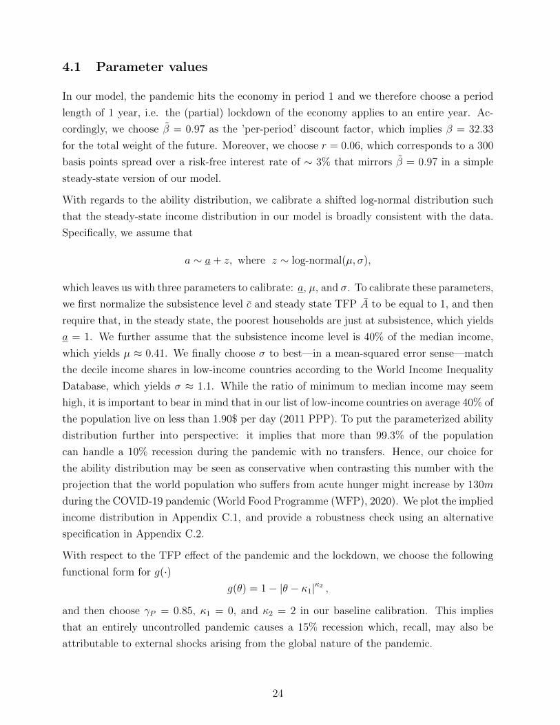
4.1 Parameter values

In our model, the pandemic hits the economy in period 1 and we therefore choose a period

length of 1 year, i.e. the (partial) lockdown of the economy applies to an entire year. Ac-˜cordingly, we choose β = 0.97 as the ’per-period’ discount factor, which implies β = 32.33

for the total weight of the future. Moreover, we choose r = 0.06, which corresponds to a 300˜basis points spread over a risk-free interest rate of ∼ 3% that mirrors β = 0.97 in a simple

steady-state version of our model.

With regards to the ability distribution, we calibrate a shifted log-normal distribution such

that the steady-state income distribution in our model is broadly consistent with the data.

Specifically, we assume that

a ∼ a+ z, where z ∼ log-normal(µ, σ),

which leaves us with three parameters to calibrate: a, µ, and σ. To calibrate these parameters,¯we first normalize the subsistence level c and steady state TFP A to be equal to 1, and then

require that, in the steady state, the poorest households are just at subsistence, which yields

a = 1. We further assume that the subsistence income level is 40% of the median income,

which yields µ ≈ 0.41. We finally choose σ to best—in a mean-squared error sense—match

the decile income shares in low-income countries according to the World Income Inequality

Database, which yields σ ≈ 1.1. While the ratio of minimum to median income may seem

high, it is important to bear in mind that in our list of low-income countries on average 40% of

the population live on less than 1.90$ per day (2011 PPP). To put the parameterized ability

distribution further into perspective: it implies that more than 99.3% of the population

can handle a 10% recession during the pandemic with no transfers. Hence, our choice for

the ability distribution may be seen as conservative when contrasting this number with the

projection that the world population who suffers from acute hunger might increase by 130m

during the COVID-19 pandemic (World Food Programme (WFP), 2020). We plot the implied

income distribution in Appendix C.1, and provide a robustness check using an alternative

specification in Appendix C.2.

With respect to the TFP effect of the pandemic and the lockdown, we choose the following

functional form for g(·)g(θ) = 1 κ− |θ − κ1| 2 ,

and then choose γP = 0.85, κ1 = 0, and κ2 = 2 in our baseline calibration. This implies

that an entirely uncontrolled pandemic causes a 15% recession which, recall, may also be

attributable to external shocks arising from the global nature of the pandemic.

24

In our model, policy impacts the pandemic via the aggregate labor supply L. We summarize

the effect of L on the pandemic and, hence, the death burden of the pandemic, by a function

P (L) = Lλ, and choose λ = 3 in our baseline calibration.

δ corresponds to the fatality rate of an uncontrolled pandemic. This may be different in

developing countries than in industrialized countries due to e.g. differences in health care,

demographics or health status. We choose δ = 0.04 in our baseline calibration, which is in

the same range but slightly higher as fatality rates assumed in the literature on industrialized

countries (Alvarez et al., 2020; Eichenbaum et al., 2020a; Glover et al., 2020). One of our

comparative statics exercises below studies the effects of a change in δ on optimal policy and

welfare.

Finally, we choose α = 0.5 in our baseline specifications, which implies a moderate consumption-

smoothing motive, but the basic pattern is very similar for alternative choices of α. We show

this in Appendix C.2 for the case of α = 1, which is consistent with our theoretical derivations

of Section 3.1.

4.2 Numerical results

We now use our numerical example to illustrate our results of the previous sections and gain

further insights on optimal policy.

Figure 1 shows welfare W , the aggregate death burden D, and compliance with the lockdown

((1 − L)/θ) in 3-D plots with θ on the x-axis and t on the y-axis. In each plot, the red

dot indicates the (unconstrained) optimal policy. These plots provide some important and

robust insights: Observe first from Figure 1a that the welfare function is single-peaked,

albeit relatively flat around the optimal policy, lending support to our discussion of first-

order conditions in the previous sections. For low levels of t, welfare is steeply increasing

in t, mirroring a declining aggregate death burden (Figure 1b) that is driven by a smaller

economic death burden on the one hand, but also a smaller pandemic death burden thanks to

improved compliance with the lockdown (Figure 1c). This suggests large welfare losses from

borrowing constraints, a point that we will return to below. Stricter lockdowns are costly for

low levels of t, but beneficial for larger levels of t, reflecting the complementarity between

these two policy variables. The optimal policy involves a sizeable lockdown of θ ∼ .3 and

transfers that amount to almost 6% of steady state GDP. The welfare loss is ∼ 3.3% and

the aggregate death burden is ∼ 1.4%. Note that both W and D become relatively flat for

high-enough t. This is when no or only very few households die from deprivation. Across

a broad set of parameter specifications this is the case for (unconstrained) optimal policy,

25

Figure 1: Policy space and key outcomes

(a) Welfare (b) Aggregate death burden

(c) Compliance

i.e. fighting the pandemic does not justify a sizeable economic death burden. Compliance is

typically below 1 and in particular also for the optimal policy, reflecting the fact that some

households cannot afford to fully comply with the lock-down.

Figure 2 depicts the effect of a borrowing constraint on policy, welfare, and the death burden.

In line with our theoretical predictions (Proposition 4), it shows that the optimal lockdown is

smaller in the constrained optimum (Figure 2a) and that, as a consequence, welfare is lower

(Figure 2b) and the aggregate death burden higher (Figure 2c). The aggregate death burden

is higher because the government has less scope both to fight the disease and to financially

support households. In fact, while in the unconstrained optimum aggregate deaths are almost

entirely accounted for by the disease, this is no longer the case with a borrowing constraint,

and Figure 2c reveals a horrible moral trade-off between saving lives from the pandemic and

rescuing poorer households from deprivation.

26

Figure 2: Optimal policy with borrowing constraint

(a) Policy (b) Welfare

(c) Aggregate death burden

Figure 3 returns to our comparative statics exercises of Section 3.1.1, but considers both

constrained and unconstrained policies. The left-hand-side panels focus on the death burden¯of the pandemic (δ), while the right-hand-side panels focus on steady state TFP (A). In

each figure, crossed out lines refer to the respective constrained optimum for b = 0.03, which

corresponds to ∼ 50% of the unconstrained optimal borrowing in our baseline specification.

Consider δ first. For δ sufficiently small, the optimum is a corner solution with θ = 0.28 For

larger δ (∼ δ > 0.01), however, the optimal θ is positive and increasing in δ, in line with

Proposition 2. As Figure 3a suggests, this is true not only for the unconstrained optimum,

but for the constrained optimum as well. Not surprisingly, welfare is smaller the larger δ both

28While this is not our main point of interest, it is nevertheless interesting that this corner solution isconsistent with the fact that e.g. governments do not fight the Influenza via lock-downs, despite the fact thatit has an estimated global annual death burden of 290’000 to 650’000 (https://www.who.int/news-room/fact-sheets/detail/influenza-(seasonal)).

27

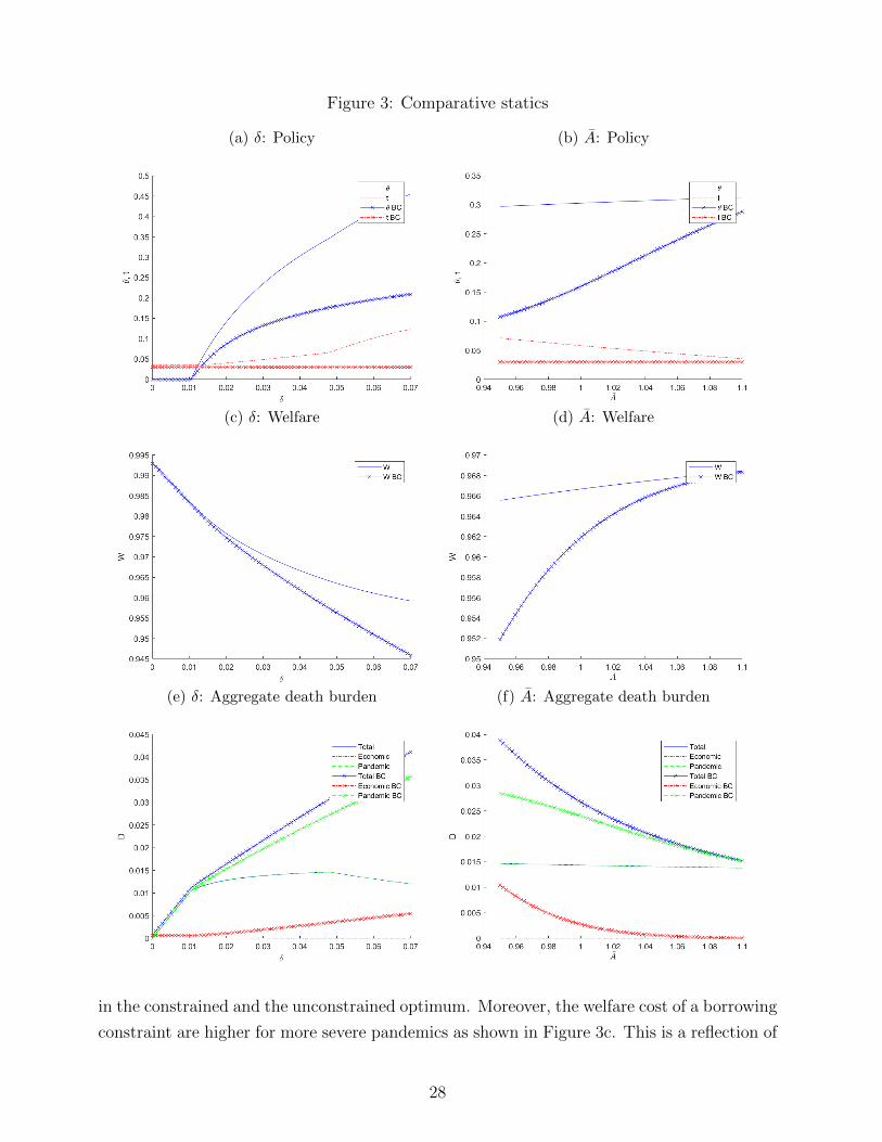
Figure 3: Comparative statics

(a) δ: Policy (b) A: Policy

(c) δ: Welfare (d) A: Welfare

(e) δ: Aggregate death burden (f) A: Aggregate death burden

in the constrained and the unconstrained optimum. Moreover, the welfare cost of a borrowing

constraint are higher for more severe pandemics as shown in Figure 3c. This is a reflection of

28

the fact that more severe pandemics justify stricter lockdowns, which are particularly costly

in the presence of a borrowing constraint. As Figure 3e shows, the death burden is larger the

higher δ and, not surprisingly, more so in the constrained than in the unconstrained optimum.

As previously discussed, in the unconstrained optimum aggregate deaths are almost entirely

accounted for by the disease, with economic deaths very small but positive. This is no longer

true in the constrained optimum. In the latter case, the government is forced to trade off

these two causes of fatalities, and this trade-off gets worse, the more severe the disease. Note

that, in the unconstrained optimum, the aggregate death rate is hump-shaped in δ. For δ

sufficiently high, economic deaths are 0, and the complementarity between θ and t implies

that the death rate in the unconstrained optimum declines in δ.

¯The right-hand side of Figure 3 considers variations in A. In line with Proposition 3, the opti-

mal θ is larger in richer countries. This is true both in the constrained and the unconstrained¯optimum. In the latter case, optimal transfers are decreasing with A, as fewer households

are endangered by deprivation. As a consequence, the gap between the constrained and the¯unconstrained optimal transfers is larger in countries with lower A, and governments in these

countries see themselves forced to more heavily cut back on the lockdown in order to pre-

vent deprivation. In other words, the gap between unconstrained and constrained optimal

policies is smaller in richer countries, both in terms of policy choices and in terms of welfare

implications, i.e. borrowing constraints are particularly costly in poor countries.

5 Robustness and Extensions

In this section, we provide further discussions. We begin with reconsidering some of our

assumptions and discuss robustness of our main insights to alternative specifications. We

then consider the distributional consequences and political economy of the pandemic.

5.1 Discussion

Our work is centered on the analysis of jointly optimal lockdowns and transfer payments and

the policy implications and welfare cost of limited fiscal space. To keep our analysis tractable

and thus build intuition of key effects at play, we make various simplifying assumptions. Yet,

our main insights are likely to prevail in alternative set-ups and might even get reinforced as

we now briefly discuss.

We take a simplistic view on fiscal policy. On the one hand, targeted transfers to support

vulnerable parts of society would improve the efficiency of fiscal policy in our model and,

29

hence, reduce the need for borrowing. Note, however, that in our model all households might

potentially benefit from the consumption-smoothing effect of transfers—more on that later.

Moreover, lump-sum transfers may be a feasible first response to an unexpected pandemic

in the absence of pre-existing more sophisticated policy instruments.29 On the other hand,

several forces tend to increase the need for fiscal space: For one thing, the global economic

shock causes a major recession and falling tax revenues. In the short-run, it may not be

feasible to 1:1 reduce precommitted government expenditures, thus increasing the need for

additional fiscal space via borrowing. For another, we do not include any direct costs of

fighting the pandemic, such as investments in the healthcare system or testing capacities,

which require additional fiscal resources. And finally, we do not consider longer-run adverse

effects of the pandemic on the economy.30 Counteracting policies such as temporary layoff

assistance or financial assistance to businesses increase the need for fiscal space even further

and tend to reinforce the complementarity between fiscal policy and a lockdown.

Similarly, a general lockdown is a blunt policy instrument, and smart testing and containment

policies (Eichenbaum et al., 2020b; Piguillem and Shi, 2020; Romer, 2020) or alternating

lockdowns (Meidan et al., 2020) may substantially improve efficiency. Nevertheless, they

are unlikely to fundamentally change the trade-offs we consider and, in fact, our reduced

form approach to modeling the pandemic as a function of aggregate labor supply may be

interpreted as reflecting such alternative containment policies.

At a general level, the role of lump-sum transfers in our model is to enable intertemporal

substitution of consumption by households. In principle, such intertemporal substitution can

also be realized via private borrowing. Yet, private borrowing may be substantially hindered

in times of uncertainty due to major health and economic shocks, and this is particularly true

for the most vulnerable parts of a society, i.e. those that are most in need of intertemporal

substitution. Moreover, note that all households would like to borrow in the first period.

Who would they be borrowing from? The rest of the world. But international contract

enforcement is difficult because the judge is in one country and the collateral (or the bailiff)

in another. For this reason, international finance is constrained.31 Indeed, the massive fiscal

stimuli and transfer payments that are put in place in countries all across the world point to

an important role of the state in facilitating intertemporal substitution.

29In either case, the possibility of targeted transfers would have qualitatively the same effect as a lower rin our model in the sense that they would lower the cost per dollar of transfers to vulnerable parts of society.

30See Barro et al. (2020) and Jorda et al. (2020) for analyses of the longer-run consequences of the Spanishflu.

31Of course, in times of a global pandemic all countries would seek to borrow, i.e. there must be somesort of borrowing from rich to poor. Nevertheless, in an ideal setting this should involve net borrowing ofpoor countries and, if such borrowing is limited due to e.g. a flight of capital to safety, this only reinforcesborrowing constraints.

30

Finally, our mechanisms might also get reinforced if we consider more than one goods. Con-

sider the case of two goods, a basic good with strictly positive subsistence consumption level

and a luxury good. Then, if a sector-specific lockdown of the luxury good sector is infeasible

or costly,32 the lockdown might put inflationary pressure on basic goods. This is because

households at or close to subsistence consumption of the basic good will increase their rela-

tive demand for the basic good during the recession, and if this increase in relative demand

is not matched by an increase in relative supply, the relative price of the basic good has to

increase to induce rich households to increase their relative demand for the luxury good.

5.2 Distributional consequences and political economy

So far, we have focused on aggregate welfare as well as distributional consequences of the

pandemic across countries. Yet, the pandemic and aggregate-welfare optimal policy have

important distributional consequences also within countries with possibly profound conse-

quences for the political economics of lockdown policies. We briefly discuss these issues next.

For our analysis of optimal policy, we did not need to take a stand on the individual risk of

dying during the pandemic. Yet, this risk is unequally distributed. Most importantly, under

the weak assumption that—ceteris paribus—households are more likely to catch the disease

the more they work,33 the probability to die is monotonically decreasing in a household’s

ability, i.e. the poor have to disproportionally bear the health burden of the pandemic.

Households also differ in their individual preferences over policies, and this has interesting

political economy implications. A detailed account of these implications is beyond the scope

of our paper and depends, among others, on the household-level probability of dying from the

disease and on how exactly the future debt-service costs are financed, which did not matter

for our analysis of Section 3.1. Nevertheless, it is informative to briefly consider the case

where α = 1 and where future debt service costs are financed via a ’flat tax’, i.e. there is no

consumption smoothing motive and the future tax burden is proportionate to income. With

these assumptions, we have the following result:

Proposition 5 (Single-crossing preferences)

Let α = 1 and suppose that future debt service costs are financed via a flat tax τ on income

32This may be because it is not politically or administratively feasible to discriminate between sectors,because a sector-level lockdown increases the need for costly redistribution (Glover et al., 2020), or becausethere are input-output linkages between the sectors (Guerrieri et al., 2020).

33Note that this is consistent with our aggregate modeling of the pandemic— Assumptions 1 and 2—if

d(a) := δ · l(a) · Lλ−1.

31

and let households with equal labor supply in period 1 have the same probability of catching

the disease. Moreover, let �a denote preferences of household a over policies. Let P denote˜the set of admissible policies p = (θ, t). Let d denote the probability of dying from the disease

of a household who fully complies with the lockdown and suppose that policies are ordered˜ ¯

according to d+ t · A· ¯ ¯µa , i.e. ph > pl ⇔ ˜ ˜dh + th · A·µa > dl + tl · A·µa· · , where here and belowβ c β c β·c

we use a superscript h (l) to denote the value of an endogenous variable given policy ph (pl).

Then, for any pair of policies ph > pl and every pair of households ah > al ≥ max{a h2 , a l

2 }it holds

pl �al ph ⇒ pl �ah ph

ph � pl ⇒ ph � plah al .

The proof of Proposition 5 is given in Appendix A.6. In words, Proposition 5 implies that the

preferences of households that can fully comply with a lockdown satisfy the single-crossing

property. It is important to note what this does—and does not—imply. It does not directly

allow to apply a median voter theorem because depending on the policy a ’median voter’

may not be able to fully comply with the lockdown and the above result does not apply. If,

however, ex-ante we restrict the set of policies such that the median voter can always fully

comply, the policy outcome in a Downsian two-party competition would be her preferred

policy. Note that this is a plausible restriction on policy: If, for example, the median income

was 250% of subsistence, it would imply that all policies were admitted that involve recessions

of ∼ 60% or less, and even deeper recessions for positive transfers. More generally, the

outcome would be the preferred policy of some decisive voter. Hence, Proposition 5 also

suggests that, ceteris paribus, we should expect to observe more intense policy measures

against the pandemic and less supporting transfers in societies where political power is in the

hands of an elite, i.e. where the decisive household is richer, and vice versa in societies with

populist governments.34

While Proposition 5 points to important conflicts of interest over policies, it is interesting to

note that providing financial support to vulnerable parts of society in times of a pandemic is

in the self-interest of households with highest ability if the negative externality of working on

the pandemic is sufficiently large and the future is sufficiently important vis-a-vis the present.

We show this in Proposition 6 where, for simplicity, we consider the case of α = 1, b = 0, i.e.

no government borrowing, and d(a) = d(P ), i.e. the risk of catching the disease only depends

on aggregate behavior. We then show that for any given θ, all households a ≥ µa are better

off providing some support to the poor in times of a pandemic if β is sufficiently large.

34There may, however, be opposing forces not captured by our model, e.g., if the elite can capture adisproportionate share of domestic income and thus has strong economic interest in keeping the economyrunning.

32

Proposition 6 (Individual gains from supporting the poor)¯Let α = 1, b = 0, d(a) = d(P ), and consider lump-sum transfers t · A · µa financed via a

contemporaneous tax proportionate to steady-state income, i.e. net transfers to household a

are t · A · [µa − ¯a]. For every θ > 0 such that µa ≥ c {A}− · > inf , there exists a β(θ) such(1 θ) A

that for β ≥ β(θ) it holds that ∣dU(a) ∣∣∣ > 0, for all a ∈ A.dt θ,t=0

The proof of Proposition 6 is given in Appendix A.7. Note that Condition µa ≥ c(1−θ)· >

A

inf{A} in Proposition 6 simply guarantees that L is decreasing in t at t = 0 by ruling out that

all households can fully comply with the lockdown and that household a2 is a net contributor

to the transfers.

6 Conclusion

In this paper, we have analyzed optimal joint policies of a lockdown and transfer payments in

times of a pandemic. We have focused on a developing country set-up and shown that both

policy instruments interact in non-trivial ways in combating the pandemic and supporting

the poor through the recession. Our work points to important distributional consequences of

the pandemic: Within countries, poorer households disproportionally die. Across countries,

combating the pandemic is costlier for poorer countries, implying that these countries suffer

from a higher death burden and a greater welfare loss. This is true with unlimited fiscal space,

and may get much worse if government borrowing is constrained. In such cases, developing

countries see themselves forced to fight less the pandemic in order to protect the poor. But

still, this may not be sufficient to save all of them from deprivation due to the multiple global

economic shocks in times of a pandemic. This is not just a theoretical possibility. Forecasts

show that COVID-19 could almost double the number of people suffering from acute hunger

(World Food Programme (WFP), 2020). In the words of Arif Husain, Chief Economist of

the World Food Programme: ’COVID-19 is potentially catastrophic for millions who are

already hanging by a thread. It is a hammer blow for millions more who can only eat if they

earn a wage. Lockdowns and global economic recession have already decimated their nest

eggs. It only takes one more shock – like COVID-19 – to push them over the edge’.35 Our

work may help clarify some of the horrible trade-offs involved, and it corroborates the urgent

calls for action to support developing countries in the COVID-19 crisis (Bolton et al., 2020;

35https://www.wfp.org/news/covid-19-will-double-number-people-facing-food-crises-unless-swift-action-taken, accessed on 5/14/2020.

33

International Monetary Fund (IMF), 2020b). This is the right thing to do. Considering the

global nature of the pandemic, it is also the smart thing to do (Hausmann, 2020).

34

Appendix

A Proofs

A.1 Proof of Proposition 1

(i) We proceed by contradiction. ∣ˆLet θ(t) be a candidate solution and suppose that dD ∣

ˆ ≥ 0. Note that this implies∣ dθ θ=θ(t)dA ∣ ˆ

ˆ < 0. This is because if θ(t) was indeed optimal, then a marginal increase in θ woulddθ θ=θ(t)

strictly lower the aggregate labor supply and, hence, the pandemic by Proposition 1(ii). As∣a consequence, dD ∣

dθ ˆ ≥ 0 requires a larger economic death burden, which in turn requiresθ=θ(t)

a lower A. Now, a larger θ weakly lowers labor supply of all households but for households

a ∈ (a1, a2] who increase their labor supply, but remain at subsistence. In combination with∣dA ∣dθ ˆ < 0, this implies that

θ=θ(t) [∫ ]d [ ]

¯v(A · a · l(a) + t · A · µa)− c · f(a)da < 0.dθ a∈A ˆθ=θ(t)

Hence, a marginal decrease in θ would strictly increase the first summand in Equation (10).∣Moreover, as dD ∣

ˆ ≥ 0 by assumption, a marginal decrease in θ would weakly increasedθ θ=θ(t)

ˆthe second summand, a contradiction to θ(t) being optimal.

(ii) We proceed by contradiction. ∣ˆLet θ(t) be a candidate solution and suppose that dL ∣ ≥ 0. Note that this implies∣ dθ ˆθ=θ(t)

dA ∣ˆ < 0, for if not, an increase in θ causes every household to decrease their labor

dθ θ=θ(t)

ˆsupply, some of them strictly. Hence, starting from θ(t), a marginal decrease in θ would

weakly decrease L and therefore P and at the same time strictly increase A. This would

strictly increase period 1 consumption of every household a ∈ A\[a1, a2) and not affect

period 1 consumption of households a ∈ [a1, a2), who remain at subsistence, i.e. they exactly

offset the higher A by a lower labor supply. It follows that[∫ ]d [ ]

¯v(A · a · l(a) + t · A · µa)− c · f(a)da < 0.dθ a∈A ˆθ=θ(t)

In addition, a marginal decrease in θ would decrease D as it weakly alleviates the pandemic∣( dL ∣ ≥ ˆ

ˆ 0), and the higher A lowers the economic death burden, a contradiction to θ(t)dθ θ=θ(t)

being optimal.

2

35

A.2 Proof of Lemma 1

Using Equation (19) in Equation (17) yields

dL dA a1 dL= · · − [1− F (a2)] .

dθ dθ A · µa dt

Using the above in Equation (16) yields

dD a1 dA dA a1 dL=− f(a1) · · · [1− d(P )] + [1− F (a1)] · δ · P ′(L) · · ·

dθ A dθ dθ A · µa dt

− [1− F (a2)] · [1− F (a1)] · δ · P ′(L) =a dA 1 dD 1 ′

1 · · · − · [1− F (a2)] · [1− F (a1)] · δ · P (L) , (A.1)dθ A · µa dt ︸a1 ︷︷ ︸

:=E

where the second equality follows from using (18). The optimal solution for θ satisfies dD = 0,dθ

which is the case when the term in the big squared brackets is 0, i.e. the result follows from∗ ∗ ˜

showing that this term is decreasing in t. Now, at (θ , t ), dW crosses 0 from above, implyingdt

that ∣d2D ∣∣∣ > 0dtdt θ=θ∗,t=t∗

and, hence, that dA · 1 dD¯ ·· is decreasing in t at t = t∗. The desired result then follows

dθ A µa dt

from the fact that E is non-decreasing in t, which implies∣d2D ∣∣∣ < 0dθdt θ=θ∗,t=t∗

and therefore ∣d2W ∣∣∣ > 0.dθdt θ=θ∗,t=t∗

To see that E is non-decreasing in t, note that [1− F (a2)] and [1− F (a1)] are both increasing

in t. Moreover,[ ′ ] [λ−1]

d P (L) d λ · L Lλ−2 dL da Lλ−11

= = λ · (λ− 1) · · − λ · · , (A.2)dt a dt a a dt dt 2

1 1 1 a1

which is positive if

dL 1 da1 1(λ− 1) · · − · ≥ 0.

dt L dt a1

¯Using Equation (19) and the fact that da1 = −A·µa yields

dt A∫ a ¯(λ− 1) · 2 µa·A · ¯− a1 a· f(a)da

A µa · A+ ≥ 0,

L a1 · A

36

which, using Equation (7) can be rearranged to yield∫ a(λ− 1) · 2 l(a) · f(a)da

a1 ≤ 1L

and, hence, is true for (θ∗, t∗) by Assumption 4.

2

A.3 Proof of Lemma 2

To show the result, we proceed by contradiction. Throughout, we consider a marginal increaseˆ ∗ ∗ ˆin δ to δ > δ, and use (θ , t ) to denote the initially optimal policy, (θ, t) to denote the new

optimal policy, and x∗ (x) the value of an endogenous variable x in the old (new) optimum.

Note first that δ does not have a direct effect on a1, a2 and, hence, L. Using Equation (9) in

the objective in decision problem (12) [ ]W = [1− ¯ ¯F (a1)− (1− F (a1)) · δ · P (L)] · A · µa − c − r · t · A · µa,

it therefore follows that for any given policy, a change in δ impacts welfare only via its direct

effect on the pandemic death burden, (1−F (a1)) · δ ·P (L). Hence, for any given policy (θ, t)

it holds [ ] [ ]˜ ˆ ˜ ¯W (θ, t; δ)−W (θ, t; δ) = − A · µa − ˆc · (1− F (a1)) · P (L) · δ − δ , (A.3)

˜ ˆwhere we used W (θ, t; δ) to denote welfare given θ, t and δ. Now, consider a policy (θ, t) and

suppose by way of contradiction that

(1− ˆF (a1)) · P (L) ≥ (1− F (a ∗1 )) · P (L∗). (A.4)

Using Equation (A.3), we get [ ]˜ ∗ ∗ ˆ − ˜ ˆ ˆ ˜W (θ , t ; δ) W (θ, t; δ) =W (θ∗ ˆ, t∗ δ)− ˜; W (θ∗, t∗; δ)− ˜ ˆ ˆ ˜ ˆW (θ, t; δ)−W (θ, t; δ)

˜+W (θ∗, t∗ ˜ ˆ; δ)−W (θ, t; δ)[ ] [ ] [ ]=− ¯ ˆA · µa − c · δ − δ · (1− F (a ∗1 )) · P (L∗)− (1− ˆF (a1)) · P (L)

˜ ∗ ∗ ˜ ˆ+W (θ , t ; δ)−W (θ, t; δ)

≥ 0, (A.5)

ˆwhere the inequality follows from Condition (A.4), δ > δ, and the optimality of (θ∗, t∗) given δ.ˆInequality (A.5) is a contradiction to (θ, t ˆ) being optimal because given δ and starting from

(θ∗, t∗), the government can increase welfare by marginally increasing θ while holding fixedˆt by Condition (20). Hence, given δ the optimal policy must involve strictly larger welfare

than when choosing (θ∗, t∗). The contradiction establishes the result.

2

37

A.4 Proof of Proposition 2

To show the result, we distinguish three cases.

(A) If given δ = 0 the optimal transfer is t∗ = 0, the result follows immediately from

Condition (20) and Lemma 1.∣(B) If dD ∣ < 0 and t∗∗ > 0, the result follows again from Condition (20) and

dtdδ t=t ,θ=θ∗,δ=0

Lemma 1. ∣(C) Finally, for the case of dD ∣ ≥ 0 and t∗∗ > 0, we consider a marginal decrease

dtdδ t=t ,θ=θ∗,δ=0

in t such that the first-order condition for t is again satisfied. We then show that given the

marginal changes in δ and t, it is beneficial to increase θ. The result then follows from

Lemma 1.

Using the implicit function theorem and recalling that we hold constant θ, we get that the

first-order condition for t continues to hold if36

2

dt d D

= − dtdδ

dδ d2 , (A.8)D

dtdt

i.e. given (A.8) we have [ ]dD d2D d2D

d = · dδ + · dt = 0. (A.9)dt dtdδ dtdt

The changes in δ and t both affect dD . In particular, using Equation (A.1), we getdθ

d2D a1 · dA 2D= dθ d· − [1− F (a2)] · [1− F (a )] · P ′1 (L) (A.10)

dθdδ A · µa dtdδ

and [¯d2D a1 · dA d2D A · dA

dθ µa dθ dD f(a2)= · − · · + · [1− F (a )] · δ · P ′(L) + ... (A.11)

dθdt ¯ 1· dtdt A ¯A µa A · µa dt 1− θ ∫ a2′ ′′ 1

+ f(a1) · [1− F (a2)] · δ · P (L)− [1− F (a2)] · [1− F (a1)] · δ · P (L) · · f(a)da,a1

a

36Differentiating Equation (18) with respect to δ and t, respectively, yields, after some straightforwardsimplifications,

2[ ∫ ]¯d D A · µ a2

a 1= · f(a1) · P (L)− [1− F (a )] · P ′1 (L) · · f(a)da (A.6)

dtdδ A a a( ) [ 1

2 ∫¯d2D A · µ a2a 1

= · f ′(a1) [1− d(P )]− 2 · f(a1) · δ · P ′(L) · · f(a)da+ ... (A.7)dtdt A a1 a[ ]∫ a2

]2′′ 1 [1− F (a1)]

+ [1− F (a1)] · δ · P (L) · f(a)da + · δ · P ′(L) · [f(a2)− f(a1)] .a1 a a1 ∣

2

Hence, both d D d2D 2

and are finite. Moreover, t∗∣

> 0 implies that d D ∣ > 0, which is the case fordtdδ dtdt dtdtθ=θ∗,t=t∗

δ = 0 if f ′(a ∗1 ) > 0.

38

where by Equation (A.1) we have

dA 1 dD 1· · = · [1− F (a2)] · [1− F (a )] · δ · P ′1 (L) (A.12)dθ A · µa dt a1

at the optimal solution. Totally differentiating dD and using dθ = 0 along with Equa-dθ

tions (A.8) to (A.12) yields[ ] 2

dD d D A · µad =− [1− F (a2)] · [1− F (a1)] · P ′(L) · dδ + dtdδ

d2 · · dδ · δ (A.13)dθ D A[ dtdt

1 f(a2)· · [1− F (a2)] · [1− F (a1)] · P ′(L) + · [1− F (a1)] · P ′(L) + ...a1 1− θ ]∫ a2 1

+ f(a1) · [1− F (a ′2)] · P (L)− [1− F (a2)] · [1− F (a ′′

1)] · P (L) · · f(a)da .a1

a

Clearly, [ ]dD

d < 0, (A.14)dθ θ=θ∗,t=t∗,δ=0

and the result follows from continuity of the above expressions in δ, t, θ.

2

A.5 Proof of Proposition 3

To show the result, we proceed in four steps. Throughout, we let (θ∗, t∗) denote the initially¯ ¯optimal policy and consider a marginal increase in A to A.

¯Step 1 The government can undo the effect of the change in A on a1, a2, and L by

lowering t while holding constant θ. In particular, a1 is constant when choosing t such that

c− t ˆ· ¯ · ¯A µa c− t∗ · A · µa= .

A A∗

ˆ ¯Using the fact that θ is held constant and, hence, that A

ˆ = A∗ , this can be rearranged to

A A[ ]∗ c 1 1

t = t − − .µ ¯a A ¯A

Clearly, a1 = a ∗1 impliesa1 a ∗1

a ∗2 = = = a2

1− θ∗ 1− θ∗ˆand, hence, L = L∗.

39

¯Step 2 For a given θ, dA · 1 does not depend on A. Hence, step 1 implies thatdθ A ∣ ∣

dL ∣ ∣∣ dL ∣∣ = ∣dθ ∗ ¯ ¯θ=θ ,t=t;A dθ θ=θ∗,t=t∗;A

and therefore ∣ ∣dD ∣ ∣∣ dD ∣∣ = ∣ ,dθ ∗ ˜ ¯θ=θ ,t=t;A dθ θ=θ∗ ¯,t=t∗;A

i.e. given t it is just optimal to not adjust θ.

¯ ¯Step 3 For a given θ, A does not depend on A. Hence, step 1 implies thatA ∣ ∣

dL ∣ ∣∣ dL ∣∣ =∗

∣dt ˜ ˆ dt ∗ ¯θ=θ ,t=t;A θ=θ ,t=t∗;A

and therefore ∣ ∣dD ∣ ∣∣ dD∣ = ∣ .dt ˆ

∣¯θ=θ∗,t=t;A dt ¯θ=θ∗,t=t∗;A

But then ∣∣ ¯ ¯dD ∣ r · A · µa r · A · µa− ∣ = > ,dt θ=θ∗

¯¯,t=t;A −c+ A · µa ˆ− ¯c+ A · µa

i.e. given θ = θ∗, the optimal t is such that [ ]> t = t∗

c 1 1t − − .

µ ¯a A ˆA

ˆStep 4 Steps 2, 3 and the complementarity between θ and t (Lemma 1) imply that θ > θ∗.

2

A.6 Proof of Proposition 5

In period 2 the proportionate income tax is used to finance the debt service costs and, hence,37

r · ¯t · A · a· ¯τ a · A = .1−D

37Strictly speaking, this expression assumes that the future ability distribution is not affected by policy,in line with our aggregate welfare analysis—see Footnote 16 for a discussion. This is not essential for theproof. More generally, it holds that

¯µ A · a¯ a r · t ·τ · a ·A = · ,

µa 1−Dwhere µa denotes the average ability in period 2 that may depend on policy. Accounting for the term µa

µa

would not affect our subsequent arguments.

40

Given policy (θ, t), the expected lifetime utility of household a ≥ a2 is therefore given by[ ]t · A · a

(1− ¯ ˜ ¯θ) · A · a+ t · A · µa − c+ (1− d) · β · A · a− r · − c1−D

˜where, as before, we use d to denote the probability of dying from the disease of a household

who fully complies with the lockdown. Now, consider a pair of policies ph > pl, and suppose

that pl �a ph for some household a ≥ max{a h2 , a l

2 }. This is the case if and only if[ ( ) ( )][ ] r · tl r · th˜a · (1− θl ¯ ˜) · Al − (1− θh) · Ah + β · A · a · (1− dl) · 1− − (1− dh) · 1−1−Dl 1−Dh( ) ( )

˜> dh − dl · β · c+ th − tl · A · µa.

Now, the right-hand side is positive and independent of a. It follows that the left-hand-side

is positive as well and, hence, increasing in a, which proves that pl � ph for every a′a′ ≥ a.

Similar arguments can be used to show the opposite case.

2

A.7 Proof of Proposition 6

¯ ¯To show the result, we derive a β(θ) such that for β ≥ β(θ), the utility of all households is

strictly increasing in t at t = 0.

Using the expression for net transfers we get for the full-compliance and the subsistence

cutoffs

¯c− t · A · µaa2 = (A.15)

(1− θ) · A− t · Ac− t · A · µa

a1 = , (A.16)A− t · A

and for aggregate labor supply∫ a2 − · ¯c t A · [µa − a]L = F (a1) + · f(a)da+ (1− θ) · [1− F (a2)]. (A.17)

a1A · a

Differentiating with respect to t and simplifying terms yields∫dL a2 A · [µa − a]

= − · f(a)da. (A.18)dt a1

A · a

Now, µa ≥ c {A}− · > inf in combination with θ > 0 implies that for t = 0 it holds that(1 θ) A

dL < 0 and a2 ≤ µa. Hence, all households a ≤ a2 are net transfer recipients and they thusdt

41

prefer any t > 0 over t = 0. Consider then households a > a2. The expected lifetime utility

of these households is given by [ ]¯ ¯U(a) = (1− θ) · A · a+ t · A · [µa − a]− c+ β · [1− d(P )] · A · a− c .

Differentiating with respect to t yields

dU(a) dL [ ]¯= A · [µa − a]− ¯β · δ · λ · Lλ−1 · · A · a− c . (A.19)

dt dt

As noted above, for t = 0 it holds that dL < 0, implying that the second summand on thedt

right-hand-side is positive while the first summand is negative for all a > µa. Hence,∣dU(a) ∣∣∣ > 0, for all a ∈ Adt θ,t=0

if the right-hand-side of Equation (A.19) is non-decreasing in a.38 Using Equations (A.15)

to (A.18), we get that this is the case if{ [ ( ) ∫ c ( ( ))]λ−1c A·(1−θ) c c

β ≥ δ · λ · F + · f(a)da+ (1− θ) · 1− FA c A · a A · (1− θ)

A

c}∫ −1

A·(1−θ) A · [µa − a]· · ¯f(a)da := β(θ).c A · aA

2

B Mathematical appendix

B.1 Motivation of P (L) convex

In this part of the appendix, we briefly motivate our choice of a convex relationship between

L and P in the context of a basic SIR model.

In our model, P (·) summarizes the effect of the pandemic on the death burden of the pan-

demic, d(P ) = δ · P . Let Itot denote the total share of the population that had the disease

once the pandemic is over and Imax the share of the population that has the disease at the

peak of the curve. Assuming that S ≈ 1 initially, i.e. almost everyone is susceptible, the

38Note that with unbounded support of F (·), this is also necessary for all households to benefit from anincrease in t in the right neighborhood of t = 0.

42

Notes: The figure depicts a stylized example of the death burden of the pandemic as a function of L. Fora given L, R0 has first been computed as R0 = 1 + 2 · L2, which implies an R0 of 3 for L = 1 and a fullcontrol of the pandemic for L = 0. Second, Itot and Imax have been computed from Equations (B.1) and(B.2). Finally, these have been used to compute d(P ) = 0.5 · I 2

max · Itot.

basic SIR model implies simple relationships between Itot, Imax and the basic reproduction

rate of infection R0 (see, e.g. Kermack et al. (1927) and Hethcote (1989))

R0 · Itot = − ln(1− Itot) (B.1)

1Imax = 1− · (1 + ln(R0)). (B.2)

R0

It further implies that the reproduction rate of the disease is quadratic in L (Alvarez et al.,

2020).39 Now, let us decompose the overall death burden into the death rate times the

fraction of the population that got infected, and let the death rate be some function h(Imax)

of the size of the peak. This yields

d(P ) = h(Imax) · Itot.

The exact shape of h(Imax) is speculative, but it is plausibly convex with limited ICUs and

a heterogeneous effect of intensive care on the death probability of infected persons.40 The

following figure takes into account these discussions and provides a stylized example of the

total death burden of the disease as a function of L. The implied relationship is indeed

convex. Further details are provided in the footer of the figure.

39This depends on the ’matching function’ between susceptibles and infected—see Garibaldi et al. (2020)and Acemoglu et al. (2020) for a discussion.

40While not directly comparable, this is nevertheless broadly consistent with the assumption of a quadraticcongestion effect in the healthcare system by Eichenbaum et al. (2020a).

43

B.2 Details on pandemic and optimal lockdown

In this part of the appendix, we argue why for a broad range of parameter values the optimal

θ is increasing in δ. We begin with some general discussions and then provide a sufficient

condition that is slack but nevertheless naturally satisfied under reasonable parameter restric-

tions. Throughout, we assume that f(a) is single-peaked, consistent with empirical income

distributions, and that it has support [1, a], where a may be infinite, i.e. we normalize ability

in terms of the lowest ability.

For any given δ, the optimal policy solves first-order conditions (13) and (14). Using Equa-

tion (A.1), the former is satisfied iff

dA 1 dD 1· · = · [1− F (a2)] · [1− F (a1)] · δ · P ′(L). (B.3)dθ A · µa dt a1

Hence, the optimal θ is increasing in δ if a marginal change in δ and t that leaves dD unchangeddt

increases the right-hand-side of the above equation. If so, it would be beneficial to increase

θ in response to this change, which implies that θ∗ must increase by Lemma 1.

Now, the first-order condition for t implies that

r · A 1 r · A 1f(a1) ≤ · ≤ · (B.4)

− ¯ ¯c+ A · µa 1− d(P ) −c+ A · µa 1− δ

which shows that a1 and f(a1) are small for reasonable values of δ and r.41 In economic

terms this is to say that the cost of saving households from deprivation during the crisis

are relatively low compared to the value of a life such that optimal policy saves the (vast)

majority of households from deprivation. In this appendix, we limit attention to the case of a

single-peaked f(·), in line with empirical income distributions. A small f(a1) then typically

implies that f ′(a1) is large relative to f(a1).42 The key point is that in such case the change

in t that is needed to rebalance first-order condition (14) is small such that the net effect of

the changes in δ and t on the right-hand-side of Equation (B.3) is positive.

The following proposition makes this point more rigorously by providing a set of sufficient

conditions for the optimal θ to increase in response to an increase in δ. As the proof shows,

this sufficient condition is clearly not necessary and the result holds for a wide range of

parameter values where this condition is not satisfied. Still, it is satisfied under reasonable

assumptions as we briefly discuss below.

41Reasonable parameter choices imply A¯ < 1. To see this note that if e.g. A = 1, i.e. there is no−c+A·µa

TFP loss in the first period, and the poorest household is just at subsistence in normal times, A¯ = 1−c+A·µa

would imply that the ratio of average to minimum income is 2.42For example, in case of a standard log-normal distribution f(x), this ratio is large for small x.

44

Proposition 7

Define k := f ′(a ∗1 ) := f(a ∗, k 1 ) , k := f(a ∗2 )1 ∗ 2 − ∗ 3 − ∗ · − ∗ . Let Assumption 4 be satisfied and

f(a1 ) [1 F (a1 )] [1 θ ] [1 F (a2 )]

suppose that f(a ∗2 ) ≥ f(a ∗1 ). Thendθ∗

> 0dδ

if δ ≤ k1

[5+k1+k2+k3]

Proof We show that Condition (A.14) is satisfied. The result then follows from Lemma 1.

Consider d2D first (see Equation (A.7)). Ignoring the last two summands on the right-hand-dtdt

side, which are positive, using that f ′(a ∗1 ) = k1 · f(a ∗1 ) and noting that43∫ a ∗2

P ′(L∗1

) · · f(a) da ≤ 2a ∗1 a

yields ∣d2

( )D ∣ ¯ 2∣ A · µa∣ ≥ · f(a ∗1 ) · [k1 − (k1 + 4) · δ].

dtdt θ A∣=θ∗,t=t∗Combining this with d2 ∣ ¯D ≤ A·µa · f(a ∗1 ) (see Equation (A.6)) we get

dtdδ ∣θ=θ∗,t=t∗ A

d2∣

D ∣∣ A ·dtdδ µ 1.

D∣ a

2 · ≤d ∣ A k1 −∗ ∗

[k1 + 4] · δdtdt θ=θ ,t=t

Consider Equation (A.13) next. Ignoring the last term in the big squared brackets, which is

negative, and using that a1 ≥ 1 along with the definitions of k1 and k2 yields that δ times

the term in big squared brackets is less than or equal to

[1− F (a ∗2 )] · [1− F (a ∗)] · P ′(L∗1 ) · δ · [1 + k2 + k3].

Taken together, this implies that[ ] [ ]dD δ · [1 + k2 + k3]

d ≤ [1− F (a ∗2 )] · [1− F (a ∗)] · P ′1 (L∗) · −1 + · dδ,dθ k1 − [k1 + 4] · δ

i.e. it is negative ifk1

δ ≤ .[5 + k1 + k2 + k3]

43Using that P ′(L) = λ · and Equation (7) yieldsL∫ ∫ a ∗a ∗ 2 ∗2 1 1 λ (λ− 1) · ∗ l (a) · f(a)da

P ′(L∗ a) · · f(a)da = · · 1 · P (L∗) ≤ 2,a a ∗a ∗ 1 λ−

11 L∗

where 1∗ ≤ 1 and P (L∗) ≤ 1. For λ ≥ 2 the inequality thus follows from Assumption 4. For λ < 2 it followsa∫ 1∗a2 da

from∗ l∗(a)·f(a)

a1

L∗ ≤ 1.

P (L)

45

2

As shown in Condition (B.4), for reasonable assumptions on r and µa, f(a1) is small. In such

cases, k1 is typically large as noted above, and the result therefore holds for a broad range

of parameter values.

B.3 Optimal lockdown with a borrowing constraint

In this part of the appendix, we provide a sufficient condition that allows to extend Propo-

sition 4(ii) to all b ≤ t∗. Our result is based on the following assumptions:

Assumption 3′

(i) g(θ) = 1− |θ − κ1|κ2 , (ii) 0 ≤ κ1 <1 ; (iii) κ2 > 12

Assumption 4′

∫ a ∗(b)(λ− 1) · 2

∗ l∗(a) · f(a)daa1 (b) ≤ 1

L∗

Assumption 5

(i) f ′(a ∗1 (b)) ≥ 0; (ii) f(a ∗2 (b)) ≥ f(a ∗1 (b))

In these assumptions, we use a ∗1 (b) (a ∗2 (b)) to denote the value of a1 (a2) given the optimal

policy with borrowing limit b. Assumption 3′ is a fairly general functional form satisfying

the conditions in Assumption 3. Assumptions 4′ is a natural extension of Assumption 4.

Assumption 5 is a weak restriction on the shape of f(·) at the cutoffs a1 and a2, which

matters for how the lockdown and transfers interact in shaping economic and pandemic

outcomes. It is always satisfied with a uniform distribution of abilities and, more generally,

tends to be true in economies with single-peaked income distributions and where the majority

of the population can afford to comply with the optimal θ. This is indeed the case for the

parameter values underlying our numerical illustration in Section 4. With these assumptions,

we can show the following result:

Proposition 4′

(ii) Let Assumptions 3′, 4′, and 5 be satisfied and suppose that b is binding. In response

to a marginal decline in b, θ∗ declines.

Proof For the purpose of this proof, let θ∗(b) and t∗(b) denote the optimal θ and t, respec-

tively, given b. The optimality of θ∗(b) implies that∣dD ∣∣∣ = 0. (B.5)dθ θ=θ∗(b)

46

2

We therefore show that d D ∣ < 0, which proves the desired result.dθdt θ=θ∗(b)

Differentiating Equation (16) with respect to t yields:

d2D ′ da1 dA 1 da1 dA 1=− f (a1) · · a1 · · · [1− d(P )]− f(a1) · · · · [1− d(P )]

dθdt ︸ dt ︷︷dθ A ︸ ︸ dt dθ︷︷ A ︸:=K :=L

dA 1 dL da1 dL+ f(a1) · a · · ′ ′

1 · δ · P (L) · − f(a1) · · δ · P (L) · (B.6)︸ dθ ︷︷A dt︸ ︸ dt ︷︷ dθ︸:=M :=N

dL dL d2L+ [1− F (a1)] · δ · P ′′(L) · · + [1− F (a ′

1)] · δ · P (L) · .︸ ︷︷ dθ dt︸ ︸ ︷︷ dθdt︸:=O :=P ∣

Recall that da1 < 0, dL < 0, P ′(L) > 0 and P ′′(L) > 0. Moreover, dA ∣∗ < 0 as discussed

dt dt dθ θ=θ (b)

in Section 3.1. At θ = θ∗(b), −K is therefore negative by Assumption 5(i). −N is negative

by Proposition 1(ii). Using Equations (16) and (B.5), we get for θ = θ∗(b):

dL da1 1L = [1− F (a1)] · δ · P ′(L) · · ·

dθ dt a1

and therefore [dL da Lλ−1

]1 dL−L + O = [1− F (a1)] · δ · · − · λ · + λ · (λ− 1) · Lλ−2 · .

dθ dt a1 dt

The term in brackets is positive as shown in the proof of Lemma 1. In combination with

Proposition 1(ii), this implies that

−L + O < 0.

¯Finally, differentiating (17) with respect to t, using da1 = −A·µa , rearranging terms, and

dt A

substituting the result in P yields[ ]¯ · ¯A µa dA 1 A · µa f(a2) dA 1 dLP = [1− F (a )] ·δ ·P ′1 (L) · · · · [f(a2)− f(a1)]− · − · ·

A dθ A A 1− θ dθ A dt

At θ = θ∗(b), the first term in the big squared brackets is negative by Assumption 5(ii).

Clearly, the last term is negative as well. Consider then the middle term, which is negative

as well. Moreover,

¯′ A · µa f(a2)

M − [1− F (a1)] · δ · P (L) · ·[ A 1− θ ]¯′ dA 1 dL A · µa f(a2)

=δ · P (L) · f(a1) · a1 · · · − [1− F (a1)] · ·dθ A dt A 1− θ[ ∫ ]

A · µ a2a a1 f(a2

=δ · P ′ dA 1 )(L) · · −f(a1) · · · · f(a)da− [1− F (a1)] ·

A dθ A a1a 1− θ

<0.

∣∣

47

The second equality follows from using Equation (19) and from rearranging terms. The

inequality follows from noting that in the third row, the term outside the big squared brackets

is positive, while the term inside these brackets is negative. To see this latter result, note first

that the first term in the big squared brackets is positive, while the second term is negative.

Second, that ∫ a2 a1[1− F (a1)] > · f(a)da.

a1a

Third, that

f(a2) ≥ f(a1)

by Assumption 5(ii). And fourth that

1 dA 1≥ − · . (B.7)1− θ dθ A

To see this last result note that

dA 1 (θ − κ1) κ2−2· |θ − κ1|− · = κ2 ·dθ A 1 θ κ κ− | − 1| 2

by Assumption 3′, which can be verified to be decreasing in κ1. Consider then the case of

κ1 = 0. In this special case, Inequality (B.7) can be rearranged to

κ2 · θκ2−1 − (κ2 − 1) · θκ2 ≤ 1.

It is easy to verify that for θ ∈ [0, 1] the left-hand-side is increasing in θ. Moreover, for θ = 1

the above condition holds with equality. This completes the proof.

2

B.4 Details on discussions of Section 3.2

Ignoring corner solutions for the sake of exposition, the first order conditions for government

decision problem (11) are∫dW ( ) dA

= v′ A · a+ t · A · µa · · a · f(a)da (B.8)dθ a∈A∫ :a≤a1

dθ [ ]′ ( ) dA dD

+ v (1− θ) · A · a+ t · A · µa · −A+ · (1− θ) · a · f(a)da+ · β · ca∈A:a2≤a dθ dθ∫ [ ( ) ( )]¯ ¯ ¯dD t · A · µa t · A · µa ′ t · A · µ− ¯ a· · ¯β v A · a− r · + r · · v A · a− r · · f(a)dadθ a∈A 1−D 1−D 1−D

=0

48

and ∫dW ′ ( )

· ¯ ¯= v A a+ t · A · µa · A · µa · f(a)da (B.9)dt a∈A∫ :a≤a1

′ ( )· · ¯+ v (1− θ) A a+ t · A · µa · A · µa · f(a)da

a∈A:a2≤∫a [ ( ) ( )]· ¯ · · ¯dD t µ t A · ¯A µa− · ¯ a

β v A · a− r · + r · · v′ t · A · µ¯ aA · a− r · · f(a)d

dt a∈A 1−D 1−D 1−D∫ ( )¯dD ′ t · A · µa ¯+ · β · ¯c− β · v A · a− r · · r · A · µa · f(a)dadt a∈A 1−D

=0,

where dD , dD , dL , and dL are as given in Equations (16) to (19). These first-order conditionsdθ dt dθ dt

can be decomposed into the following effects:

Recession effect of a lockdown:∫ ( ) dA¯v′ A · a+ t · A · µa · · a · f(a)daa∈A∫ :a≤a1

dθ [ ]( ) dA¯+ v′ (1− θ) · A · a+ t · A · µa · −A+ · (1− θ) · a · f(a)daa∈A:a2≤a dθ

Value-of-life effect: [ ∫ ( ) ]¯dD t · A · µa− · −β · ¯c+ β · v A · a− r · · f(a)dadθ a∈A 1−D

Debt-burden effect: ∫ ( )¯ ¯dD t · A · µa ′ t · A · µa− · r · · ¯β · v A · a− r · · f(a)dadθ a∈A 1−D 1−D

Consumption-smoothing effect of transfers:∫′ ( )v A · · ¯ · · ¯a+ t A µa A · µa · f(a)da

a∈A∫ :a≤a1 ( )¯ ¯+ v′ (1− θ) · A · a+ t · A · µa · A · µa · f(a)da

a∈A∫ :a2≤a ( )· ¯t A · µa− β · ′ ¯ · − · ¯v A a r · r · A · µa · f(a)da

a∈A 1−D

We discuss these effects and their implications for our comparative statics results in Sec-

tion 3.2. In these discussions, we make further use of the fact that the marginal benefit of a

lower D as jointly captured by the value-of-life and the debt-burden effect[ ∫ ( ) ( ) ]· ¯ · ¯ ¯t A µa t · A · µa t · A · µ¯ ¯ a

β · −c+ v A · a− r · + r · · v′ A · a− r · · f(a)daa∈A 1−D 1−D 1−D

a

49

is increasing in t and D. This immediately follows from the fact that for any concave function

v(x)

v(x− ε) + ε · v′(x− ε)

is increasing in ε.

C Details on the numerical example

In this part of the appendix, we provide further details on the numerical example of Section 4.

C.1 Details on the ability distribution

To calibrate the ability distribution, we assume that it follows a shifted log-normal distribu-

tion

a ∼ a+ z, z ∼ log-normal(µ, σ),

where a = 1 as explained in Section 4. We then use the ratio of median to subsistence income,

φ. With a shifted log-normal distribution this is given by

median(a) a+ exp(µ)φ := =

a a

and, hence, allows to calibrate µ as

µ = ln(φ− 1) + ln(a),

which yields µ ≈ 0.41. Finally, we choose σ to minimize

10 [ ]∑ s 2i − si

min ,σ sii=1

where si and si are the income shares of the ith decile in the data and for our fitted distri-

bution, respectively. To reduce measurement error in the income distribution for developing

countries, we use the average decile shares across all low-income countries for which these

shares are included in the World Income Inequality Database (UNU-WIDER, 2019).44 This

yields σ ≈ 1.1.

Figure 4 depicts the implied ability distribution and Table 1 shows the actual and the fitted

decile shares.

44Specifically, we include all countries that report these shares for at least one year from 2012 onwardsand take for each country the latest available observation.

50

Figure 4: Fitted ability distribution

Notes: The figure depicts the fitted ability distribution used in the baseline calibration of our model:

a ∼ 1 + z, z ∼ log-normal(0.41, 1.1)

Table 1: Actual and fitted decile shares

s1 s2 s3 s4 s5 s6 s7 s8 s9 s10

actual 0.026 0.039 0.049 0.058 0.068 0.080 0.095 0.116 0.152 0.318fitted 0.033 0.039 0.046 0.053 0.061 0.073 0.088 0.111 0.154 0.342

C.2 Alternative parameter specifications

In this part of the appendix, we provide robustness checks for our numerical illustration.

Specifically, we show the counterparts of Figures 1 to 3, first for the case of α = 1, which

we considered in Section 3.1, and second for an alternative fitted ability distribution. In this

alternative, the ratio of median to minimum income is 3.5, which implies µ = 0.92, σ = 0.97.

All other parameter values are as in our baseline calibration.

51

C.2.1 α = 1

Figure 5: Policy space and key outcomes (α = 1)

(a) Welfare (b) Aggregate death burden

(c) Compliance

52

Figure 6: Optimal policy with borrowing constraint (α = 1)

(a) Policy (b) Welfare

(c) Aggregate death burden

53

Figure 7: Comparative statics (α = 1)

(a) δ: Policy (b) A: Policy

(c) δ: Welfare (d) A: Welfare

(e) δ: Aggregate death burden (f) A: Aggregate death burden

54

C.2.2 µ = 0.92, σ = 0.97

Figure 8: Policy space and key outcomes (µ = 0.92, σ = 0.97)

(a) Welfare (b) Aggregate death burden

(c) Compliance

55

Figure 9: Optimal policy with borrowing constraint (µ = 0.92, σ = 0.97)

(a) Policy (b) Welfare

(c) Aggregate death burden

56

Figure 10: Comparative statics (µ = 0.92, σ = 0.97)

(a) δ: Policy (b) A: Policy

(c) δ: Welfare (d) A: Welfare

(e) δ: Aggregate death burden (f) A: Aggregate death burden

57

References

Acemoglu, D., Chernozhukov, V., Werning, I., and Whinston, M. D. (2020). A multi-risk

SIR model with optimally targeted lockdown. Working Paper 27102, National Bureau of

Economic Research.

Aizenman, J., Kletzer, K., and Pinto, B. (2007). Economic growth with constraints on

tax revenues and public debt: Implications for fiscal policy and cross-country differences.

Working Paper 12750, National Bureau of Economic Research.

Alon, T. M., Kim, M., Lagakos, D., and VanVuren, M. (2020). How should policy responses

to the COVID-19 pandemic differ in the developing world? Working Paper 27273, National

Bureau of Economic Research.

Alvarez, F. E., Argente, D., and Lippi, F. (2020). A simple planning problem for COVID-19

lockdown. Working Paper 26981, National Bureau of Economic Research.

Atkeson, A. (2020). What will be the economic impact of COVID-19 in the US? Rough esti-

mates of disease scenarios. Working Paper 26867, National Bureau of Economic Research.

Baqaee, D. R. and Farhi, E. (2020). Supply and demand in disaggregated Keynesian

economies with an application to the Covid-19 crisis. Discussion Paper 14743, Centre

for Economic Policy Research.

Barro, R. J., Ursua,´ J. F., and Weng, J. (2020). The Coronavirus and the great influenza pan-

demic: Lessons from the ’Spanish Flu’ for the Coronavirus’ potential effects on mortality

and economic activity. Working Paper 26866, National Bureau of Economic Research.

Bell, C., Devarajan, S., and Gersbach, H. (2006). The long-run economic costs of Aids: A

model with an application to South Africa. The World Bank Economic Review, 20(1):55–

89. Publisher: Oxford Academic.

Besley, T. and Persson, T. (2009). The origins of state capacity: Property rights, taxation,

and politics. American Economic Review, 99(4):1218–1244.

Bigio, S., Zhang, M., and Zilberman, E. (2020). Transfers vs credit policy: Macroeconomic

policy trade-offs during Covid-19. Working Paper 27118, National Bureau of Economic

Research.

Bloom, D. E. and Canning, D. (2006). Epidemics and economics. Pontifical Academy of

Sciences, Scripta Varia, 106.

58

Bodenstein, M., , Corsetti, G., and Guerrieri, L. (2020). Social distancing and supply disrup-

tions in a pandemic. Finance and Economics Discussion Series 2020-031, Federal Reserve

Board. Divisions of Research & Statistics and Monetary Affairs.

Bolton, P., Buchheit, L., Gourinchas, P.-O., Hsieh, C.-T., Panizza, U., and di Mauro, B. W.

(2020). Born out of necessity: A debt standstill for COVID-19. Centre for Economic Policy

Research Policy Insight, (103).

Bulow, J. and Rogoff, K. (1989). Sovereign debt: Is to forgive to forget? The American

Economic Review, 79(1):43–50.

Caballero, R. J. and Krishnamurthy, A. (2001). International and domestic collateral con-

straints in a model of emerging market crises. Journal of Monetary Economics, 48:513–548.

Caballero, R. J. and Simsek, A. (2020). A model of asset price spirals and aggregate demand

amplification of a COVID-19 shock. Working Paper 27044, National Bureau of Economic

Research.

Case, A. and Deaton, A. (2020). Deaths of Despair and the Future of Capitalism. Princeton

University Press, Princeton, NJ.

Cespedes, L. F., Chang, R., and Velasco, A. (2020). The macroeconomics of a pandemic: A

minimalist model. Working Paper 27228, National Bureau of Economic Research.

Chang, R. and Velasco, A. (2020). Economic policy incentives to preserve lives and liveli-

hoods. Working Paper 27020, National Bureau of Economic Research.

Chari, V. V., Dovis, A., and Kehoe, P. J. (2020). On the optimality of financial repression.

Journal of Political Economy, 128(2):710–739.

Eichenbaum, M., Rebelo, S., and Trabandt, M. (2020a). The macroeconomics of epidemics.

Working Paper 26882, National Bureau of Economic Research, Cambridge, MA.

Eichenbaum, M. S., Rebelo, S., and Trabandt, M. (2020b). The macroeconomics of testing

and quarantining. Working Paper 27104, National Bureau of Economic Research.

Eichengreen, B., Hausmann, R., and Panizza, U. (2007). Currency mismatches, debt intoler-

ance, and the original sin: Why they are not the same and why it matters. In Edwards, S.,

editor, Capital Controls and Capital Flows in Emerging Economies: Policies, Practices,

and Consequences, pages 121–170. University of Chicago Press, Chicago, IL.

59

Farboodi, M., Jarosch, G., and Shimer, R. (2020). Internal and external effects of social

distancing in a pandemic. Working Paper 27059, National Bureau of Economic Research.

Faria-e-Castro, M. (2020). Fiscal policy during a pandemic. SSRN Scholarly Paper 3587693,

Social Science Research Network.

Garibaldi, P., Moen, E. R., and Pissarides, C. A. (2020). Modelling contacts and transitions

in the SIR epidemics model. COVID Economics, (5):120.

Gavin, M. and Perotti, R. (1997). Fiscal policy in Latin America. NBER Macroeconomics

Annual, 12:11–72.

Gersbach, H., Schetter, U., and Schneider, M. T. (2019). Taxation, innovation and en-

trepreneurship. The Economic Journal, 129(620):1731–1781.

Glover, A., Heathcote, J., Krueger, D., and Rıos-Rull, J.-V. (2020). Health versus wealth:

On the distributional effects of controlling a pandemic. Working Paper 27046, National

Bureau of Economic Research.

Gourinchas, P.-O. (2020). Flattening the pandemic and recession curves. In Baldwin, R.

and di Mauro, B. W., editors, Mitigating the COVID Economic Crisis: Act Fast and Do

Whatever It Takes. CEPR Press, London, UK.

Greenwood, J., Kircher, P., Santos, C., and Tertilt, M. (2019). An Equilibrium Model of the

African HIV/AIDS Epidemic. Econometrica, 87(4):1081–1113.

Guerrieri, V., Lorenzoni, G., Straub, L., and Werning, I. (2020). Macroeconomic implications

of COVID-19: Can negative supply shocks cause demand shortages? Working Paper 26918,

National Bureau of Economic Research.

Hall, R. E., Jones, C. I., and Klenow, P. J. (2020). Trading off consumption and COVID-19

deaths. Mimeo. https://web.stanford.edu/∼chadj/Consumption v Covid.pdf.

Hausmann, R. (2020). Flattening the COVID-19 curve in developing countries. Project

Syndicate. https://www.project-syndicate.org/commentary/flattening-covid19-curve-in-

developing-countries-by-ricardo-hausmann-2020-03.

Hethcote, H. W. (1989). Three basic epidemiological models. In Levin, S. A., Levin, S. A.,

Hallam, T. G., and Gross, L. J., editors, Applied Mathematical Ecology, volume 18, pages

119–144. Springer, Berlin, Heidelberg.

60

Hevia, C. and Neumeyer, P. A. (2020). A perfect storm: COVID-19 in emerging economies.

VoxEU. https://voxeu.org/article/perfect-storm-covid-19-emerging-economies.

International Monetary Fund (IMF) (2020a). Fiscal Monitor. Policies to support people

during the COVID-19 pandemic. https://www.imf.org/en/Publications/FM/Issues/2020/

04/06/fiscal-monitor-april-2020.

International Monetary Fund (IMF) (2020b). World Bank Group and IMF mobilize partners

in the fight against COVID-19 in Africa. Press Release 20/168.

Jones, C. J., Philippon, T., and Venkateswaran, V. (2020). Optimal mitigation policies in

a pandemic: Social distancing and working from home. Working Paper 26984, National

Bureau of Economic Research.

`Jorda, O., Singh, S. R., and Taylor, A. M. (2020). Longer-run economic consequences of

pandemics. Working Paper 2020-09, Federal Reserve Bank of San Francisco.

Kaminsky, G. L., Reinhart, C. M., and Vegh, C. A. (2004). When it rains, it pours: Procycli-

cal capital flows and macroeconomic policies. NBER Macroeconomics Annual, 19:11–53.

Kermack, W. O., McKendrick, A. G., and Walker, G. T. (1927). A contribution to the

mathematical theory of epidemics. Proceedings of the Royal Society of London. Series A,

Containing Papers of a Mathematical and Physical Character, 115(772):700–721.

Krueger, D., Uhlig, H., and Xie, T. (2020). Macroeconomic dynamics and reallocation in an

epidemic. Discussion Paper 14607, Centre for Economic Policy Research.

Loayza, N. V. (2020). Costs and tradeoffs in the fight against the COVID-19 pandemic: A

developing country perspective. Research & Policy Briefs from the World Bank Malaysia

Hub 35, World Bank Group.

Loayza, N. V. and Pennings, S. (2020). Macroeconomic policy in the time of COVID-19: A

primer for developing countries. Research & Policy Briefs from the World Bank Malaysia

Hub 28, World Bank Group.

Meidan, D., Schulamann, N., Cohen, R., Haber, S., Yaniv, E., Sarid, R., and

Barzel, B. (2020). Alternating quarantine for sustainable mitigation of COVID-19.

arxiv:2004.01453v2 [q-bio.pe].

Piguillem, F. and Shi, L. (2020). Optimal COVID-19 quarantine and testing policies. Working

Paper 20/04, Einaudi Institute for Economics and Finance (EIEF).

61

Rampini, A. A. (2020). Sequential lifting of COVID-19 interventions with population het-

erogeneity. Working Paper 27063, National Bureau of Economic Research.

Ray, D., Subramanian, S., and Vandewalle, L. (2020). India’s lockdown. Centre for Economic

Policy Research Policy Insight, (102).

Romer, P. (2020). Roadmap to responsibly reopen America. Report.

Stiglitz, J. E. and Weiss, A. (1981). Credit rationing in markets with imperfect information.

The American Economic Review, 71(3):393–410.

Sturzenegger, F. (2020). A note on hibernation in a lockdown. Working Paper 137, Univer-

sidad de San Andres.

UNU-WIDER (2019). World income inequality database (WIID). 17 December 2019.

von Carnap, T., Almas, I., Bold, T., Ghisolfi, S., and Sandefur, J. (2020). The macroeco-

nomics of pandemics in developing countries: an application to uganda. Mimeo, Stockholm

University.

World Food Programme (WFP) (2020). COVID-19. External situation report. Technical

Report 7.

62