GEOMETRICAL MOTION PLANNING FOR

HIGHLY REDUNDANT MANIPULATORS

USING A CONTINUOUS MODEL

APPROVED BY

SUPERVISORY COMMITTEE:

To my family: Sumiko, Ayako, and Yu

GEOMETRICAL MOTION PLANNING FOR

HIGHLY REDUNDANT MANIPULATORS

USING A CONTINUOUS MODEL

by

AKIRA HAYASHI, B.S.,M.S.

DISSERTATION

Presented to the Faculty of the Graduate School of

The University of Texas at Austin

in Partial Ful�llment

of the Requirements

for the Degree of

DOCTOR OF PHILOSOPHY

THE UNIVERSITY OF TEXAS AT AUSTIN

August, 1994

Acknowledgments

I would like to extend my deepest gratitude to my advisor Dr. Ben-

jamin J. Kuipers for his advice, encouragements, and supports. Without his

help, this doctoral research could not have been completed.

I am also grateful to Dr. Donald S. Fussell, Dr. Robert A. van de Geijn,

Dr. Raymond J. Mooney, and Dr. Robert A. Freeman for their serving as the

committee members.

Many thanks to my friends, Chris Walton and Richard Froom for

taking on the tiresome work of proofreading this dissertation, and to David

Throop for his development of POS: the PostScripting facility which was used

to include many of the �gures in this dissertation.

AKIRA HAYASHI

The University of Texas at Austin

August, 1994

iv

GEOMETRICAL MOTION PLANNING FOR

HIGHLY REDUNDANT MANIPULATORS

USING A CONTINUOUS MODEL

Publication No.

Akira Hayashi, Ph.D.

The University of Texas at Austin, 1991

Supervising Professor: Benjamin J. Kuipers

There is a need for highly redundant manipulators to work in com-

plex, cluttered environments. Our goal is to plan paths for such manipulators

e�ciently.

The path planning problem has been shown to be PSPACE-complete

in terms of the number of degrees of freedom (DOF) of the manipulator. We

present a method which overcomes the complexity with a strong heuristic:

utilizing redundancy by means of a continuous manipulator model. The con-

tinuous model allows us to change the complexity of the problem from a func-

tion of both the DOF of the manipulator (believed to be exponential) and the

complexity of the environment (polynomial), to a polynomial function of the

complexity of the environment only.

v

The power of the continuous model comes from the ability to decom-

pose the manipulator into segments, with the number, size, and boundaries

of the segments varying smoothly and dynamically. First, we develop motion

schemas for the individual segments to achieve a basic set of goals in open and

cluttered space. Second, we plan a smooth trajectory through free space for a

point robot with a maximum curvature constraint. Third, the path generates a

set of position subgoals for the continuous manipulator which are achieved by

the basic motion schemas. Fourth, the mapping from the continuous model to

an available jointed arm provides the curvature bound and obstacle envelopes

required (in step 2) to guarantee a collision-free path.

The validity of the continuous model approach is also supported by

an extensive simulation which we performed. While the simulation has been

performed in 2-D, we show a natural extension to 3-D for each technique we

have implemented for the 2-D simulation.

vi

Table of Contents

Acknowledgments iv

Table of Contents vii

List of Tables xii

List of Figures xiii

1. Introduction 1

1.1 Motivation : : : : : : : : : : : : : : : : : : : : : : : : : : : : : : 1

1.2 Highly Redundant Manipulators : : : : : : : : : : : : : : : : : : 4

1.3 Limitations of the Current Path Planning Algorithms : : : : : : 7

1.4 Utilizing Redundancy for Obstacle Avoidance : : : : : : : : : : 8

1.5 Swan's Neck Scenario for Path Planning : : : : : : : : : : : : : 9

1.6 Overview of Our Approach : : : : : : : : : : : : : : : : : : : : : 10

1.7 Related Work : : : : : : : : : : : : : : : : : : : : : : : : : : : : 13

2. Current Approaches to Path Planning 14

2.1 Task Level Programming : : : : : : : : : : : : : : : : : : : : : : 14

2.2 Complexity of Path Planning Problems : : : : : : : : : : : : : : 17

2.3 Con�guration Space Approach : : : : : : : : : : : : : : : : : : : 18

2.4 Heuristic Con�guration Space Approach : : : : : : : : : : : : : 20

2.5 Arti�cial Potential Field Approach : : : : : : : : : : : : : : : : 22

2.6 Hybrid Approaches : : : : : : : : : : : : : : : : : : : : : : : : : 25

vii

2.7 Summary of the Chapter : : : : : : : : : : : : : : : : : : : : : : 27

3. The Continuous Manipulator Model 28

3.1 Why a Continuous Model? : : : : : : : : : : : : : : : : : : : : : 28

3.2 Intrinsic Properties of Plane Curves : : : : : : : : : : : : : : : : 29

3.2.1 Regular Curves : : : : : : : : : : : : : : : : : : : : : : : 30

3.2.2 Curve Length : : : : : : : : : : : : : : : : : : : : : : : : 30

3.2.3 Curvature : : : : : : : : : : : : : : : : : : : : : : : : : : 31

3.2.4 Existence of a Plane Curve given Curvature : : : : : : : 32

3.2.5 Frenet Equations : : : : : : : : : : : : : : : : : : : : : : 33

3.3 Continuous Model in 2-D : : : : : : : : : : : : : : : : : : : : : : 34

3.3.1 Curvature Segment and Curvature Operators : : : : : : 34

3.3.2 Decomposition of Segment : : : : : : : : : : : : : : : : : 35

3.3.3 Obtaining a Con�guration from Curvature : : : : : : : : 37

3.4 Intrinsic Properties of Space Curves : : : : : : : : : : : : : : : : 39

3.4.1 Regular Curve : : : : : : : : : : : : : : : : : : : : : : : : 40

3.4.2 Curve Length : : : : : : : : : : : : : : : : : : : : : : : : 40

3.4.3 Curvature : : : : : : : : : : : : : : : : : : : : : : : : : : 40

3.4.4 Torsion : : : : : : : : : : : : : : : : : : : : : : : : : : : 41

3.4.5 Existence of a Space Curve given Curvature and Torsion 42

3.5 Continuous Model in 3-D : : : : : : : : : : : : : : : : : : : : : : 43

4. Solving Open Space Problems 45

4.1 Open Space Problems : : : : : : : : : : : : : : : : : : : : : : : : 45

4.1.1 Four Types of Open Space Problems : : : : : : : : : : : 45

4.1.2 The Swan's Neck Simulator : : : : : : : : : : : : : : : : 46

viii

4.2 Hill Climbing Searches : : : : : : : : : : : : : : : : : : : : : : : 47

4.3 Solving the Local Minima Problem : : : : : : : : : : : : : : : : 50

4.3.1 The Local Minima Problem : : : : : : : : : : : : : : : : 50

4.3.2 Typical Con�gurations : : : : : : : : : : : : : : : : : : : 52

4.3.3 Interpolation to a Good Initial Con�guration : : : : : : : 53

4.3.4 Simulation Results : : : : : : : : : : : : : : : : : : : : : 56

4.4 Related Work on Inverse Kinematics : : : : : : : : : : : : : : : 56

4.4.1 Redundant Jointed Arms : : : : : : : : : : : : : : : : : : 56

4.4.2 Continuous Arms : : : : : : : : : : : : : : : : : : : : : : 58

4.4.3 Research on Curve Design : : : : : : : : : : : : : : : : : 59

4.5 Summary of the Chapter : : : : : : : : : : : : : : : : : : : : : : 60

5. Basic Motion Schemas for Path Planning 64

5.1 The Basic Motion Schemas : : : : : : : : : : : : : : : : : : : : : 64

5.1.1 Motion Schemas for Open Space : : : : : : : : : : : : : : 65

5.1.2 Motion Schemas for Cluttered Space : : : : : : : : : : : 66

5.2 Using Motion Schemas with Decomposition : : : : : : : : : : : : 67

5.3 Path Planning Problem for the Continuous Manipulator : : : : 68

5.3.1 Where Do We Start? : : : : : : : : : : : : : : : : : : : : 70

5.3.2 Remaining Problems : : : : : : : : : : : : : : : : : : : : 73

5.3.3 Our Approach : : : : : : : : : : : : : : : : : : : : : : : : 74

6. Planning a Smooth Path for Autonomous Vehicles using Pri-

mary Convex Regions 76

6.1 Introduction : : : : : : : : : : : : : : : : : : : : : : : : : : : : : 76

6.2 Free Space Decomposition : : : : : : : : : : : : : : : : : : : : : 77

ix

6.2.1 Free Space Decomposition Methods : : : : : : : : : : : : 78

6.2.2 Primary Convex Regions : : : : : : : : : : : : : : : : : : 79

6.2.3 Hypergraph Method for Finding PCRs : : : : : : : : : : 80

6.3 Making a Smooth Turn between PCRs : : : : : : : : : : : : : : 81

6.3.1 Candidate Turning Corners : : : : : : : : : : : : : : : : 81

6.3.2 Cubic Spirals : : : : : : : : : : : : : : : : : : : : : : : : 82

6.3.3 Making Smooth Turns using Cubic Spiral Curves : : : : 83

6.4 Graph Search for a Smooth Path : : : : : : : : : : : : : : : : : 86

6.4.1 Connectivity Graph : : : : : : : : : : : : : : : : : : : : : 86

6.4.2 A� Search : : : : : : : : : : : : : : : : : : : : : : : : : : 87

6.4.3 Complexity : : : : : : : : : : : : : : : : : : : : : : : : : 88

6.4.4 Experimental Results : : : : : : : : : : : : : : : : : : : : 89

6.5 Summary : : : : : : : : : : : : : : : : : : : : : : : : : : : : : : 90

6.6 Related Work : : : : : : : : : : : : : : : : : : : : : : : : : : : : 93

7. Path Planning for the Continuous Manipulator 95

7.1 Achieving Subgoals along a Smooth Path : : : : : : : : : : : : : 95

7.1.1 Finding Subgoals : : : : : : : : : : : : : : : : : : : : : : 95

7.1.2 Achieving Subgoals : : : : : : : : : : : : : : : : : : : : : 96

7.1.3 Comment on the Meaning of Convexity : : : : : : : : : : 99

7.2 Extend to 3-D : : : : : : : : : : : : : : : : : : : : : : : : : : : : 99

7.2.1 2 + 12-D Approach : : : : : : : : : : : : : : : : : : : : : : 100

7.2.2 About Hypergraph Method : : : : : : : : : : : : : : : : 101

7.3 3-D free space decomposition : : : : : : : : : : : : : : : : : : : 102

7.3.1 Singh and Wang's method to �nd Primary Convex Regions102

7.3.2 Finding Primary Convex Regions in 3-D : : : : : : : : : 105

x

7.3.3 Free Space Partitioning Methods : : : : : : : : : : : : : 110

8. Mapping the Solution to a Jointed Arm 112

8.1 Every-Other-Joint Mapping : : : : : : : : : : : : : : : : : : : : 112

8.2 Evaluating Mapping Errors : : : : : : : : : : : : : : : : : : : : 113

8.2.1 Single Arc Case : : : : : : : : : : : : : : : : : : : : : : : 118

8.2.2 Tangent Arcs Case : : : : : : : : : : : : : : : : : : : : : 123

8.2.3 Proposition for Error Bound : : : : : : : : : : : : : : : : 125

8.3 Improving the Approximation : : : : : : : : : : : : : : : : : : : 128

8.4 Dynamic Simulation of the Swan's Neck Manipulator : : : : : : 129

9. Summary and Conclusions 131

9.1 Summary : : : : : : : : : : : : : : : : : : : : : : : : : : : : : : 131

9.2 Comparison with Other Approaches : : : : : : : : : : : : : : : : 132

9.2.1 Complexity in terms of DOF : : : : : : : : : : : : : : : : 133

9.2.2 When We Fix DOF : : : : : : : : : : : : : : : : : : : : : 134

9.2.3 Search Space for Our Approach : : : : : : : : : : : : : : 135

9.2.4 Ruler Folding Problem : : : : : : : : : : : : : : : : : : : 135

9.2.5 Advantage of Our Approach : : : : : : : : : : : : : : : : 136

9.3 Future Work : : : : : : : : : : : : : : : : : : : : : : : : : : : : : 138

9.3.1 3-D Simulation : : : : : : : : : : : : : : : : : : : : : : : 138

9.3.2 Building/Controlling a Highly Redundant Manipulator : 139

9.4 Contributions : : : : : : : : : : : : : : : : : : : : : : : : : : : : 140

BIBLIOGRAPHY 142

Vita

xi

List of Tables

4.1 Four Types of Open Space Problems : : : : : : : : : : : : : : : 46

6.1 Search Time and Path Length : : : : : : : : : : : : : : : : : : : 92

xii

List of Figures

1.1 Path Planning Problem : : : : : : : : : : : : : : : : : : : : : : : 2

1.2 Redundancy Helps to Avoid Obstacles : : : : : : : : : : : : : : 3

1.3 Scenario for Achieving Goal Position : : : : : : : : : : : : : : : 9

1.4 Overview of the Motion Planning System : : : : : : : : : : : : : 11

1.5 Solution Sequence of Our Approach : : : : : : : : : : : : : : : : 12

2.1 Task Space and Con�guration Space : : : : : : : : : : : : : : : 18

2.2 Obstacles in Con�guration Space : : : : : : : : : : : : : : : : : 19

2.3 Arti�cial Potential Field : : : : : : : : : : : : : : : : : : : : : : 23

2.4 Getting Caught in a Local Minimum : : : : : : : : : : : : : : : 24

3.1 Osculating Circle and Radius of Curvature : : : : : : : : : : : : 32

3.2 Tangent and Normal Vectors : : : : : : : : : : : : : : : : : : : : 33

3.3 Curvature Segment Representation and its Operators : : : : : : 35

3.4 Decomposition of Segment : : : : : : : : : : : : : : : : : : : : : 36

3.5 Tangent, Normal, and Binormal Vectors : : : : : : : : : : : : : 42

4.1 Simulation Window : : : : : : : : : : : : : : : : : : : : : : : : : 47

4.2 Curvature Segment Representation and its Operators : : : : : : 48

4.3 Polar Coordinates for Distance Functions : : : : : : : : : : : : : 50

xiii

4.4 Successful Hill-Climbing : : : : : : : : : : : : : : : : : : : : : : 51

4.5 Local Minimum in Hill Climbing : : : : : : : : : : : : : : : : : : 51

4.6 Curvature Segment Type : : : : : : : : : : : : : : : : : : : : : : 53

4.7 Curvature Segment Types in �-� Plane : : : : : : : : : : : : : : 54

4.8 Five Candidate Initial Con�gurations : : : : : : : : : : : : : : : 55

4.9 Interpolate to Good Initial Con�guration and Hill Climbing : : 55

4.10 Example 1 as OSP1 : : : : : : : : : : : : : : : : : : : : : : : : : 62

4.11 Example 1 as OSP2 : : : : : : : : : : : : : : : : : : : : : : : : : 62

4.12 Example 1 as OSP3 : : : : : : : : : : : : : : : : : : : : : : : : : 62

4.13 Example 1 as OSP4 : : : : : : : : : : : : : : : : : : : : : : : : : 62

4.14 Example 2 as OSP4 : : : : : : : : : : : : : : : : : : : : : : : : : 63

4.15 Example 3 as OSP4 : : : : : : : : : : : : : : : : : : : : : : : : : 63

5.1 Feed/Retract Motion Schemas : : : : : : : : : : : : : : : : : : : 66

5.2 Fold/Unfold Motion Schemas : : : : : : : : : : : : : : : : : : : 67

5.3 Motion Plan Representation : : : : : : : : : : : : : : : : : : : : 67

5.4 Fold, Rotate, and Extend a Manipulator : : : : : : : : : : : : : 69

5.5 Overview of the Motion Planning System : : : : : : : : : : : : : 71

5.6 Visibility Graph Method To Find a Polygonal Path : : : : : : : 72

5.7 Grow Obstacles : : : : : : : : : : : : : : : : : : : : : : : : : : : 75

6.1 Wall Segments and Primary Convex Regions : : : : : : : : : : : 79

xiv

6.2 Candidate Turning Corners : : : : : : : : : : : : : : : : : : : : 81

6.3 Cubic Spirals and Circles : : : : : : : : : : : : : : : : : : : : : : 82

6.4 Making a Smooth Turn using a Cubic Spiral : : : : : : : : : : : 84

6.5 dfreemax and dfitmax : : : : : : : : : : : : : : : : : : : : : : : : : : : : 85

6.6 Steps Involved in Path Planning : : : : : : : : : : : : : : : : : : 87

6.7 Paths Found : : : : : : : : : : : : : : : : : : : : : : : : : : : : : 88

6.8 Maximal Overlapping Regions and Road Map : : : : : : : : : : 90

6.9 Smooth Paths Found for 4 Environments : : : : : : : : : : : : : 91

7.1 Path Planning for Manipulator : : : : : : : : : : : : : : : : : : 97

7.2 Retract, Rotate, and Extend : : : : : : : : : : : : : : : : : : : : 98

7.3 Fuse Free Regions in 2-D : : : : : : : : : : : : : : : : : : : : : : 103

7.4 Fuse Free Regions in 2-D and 3-D : : : : : : : : : : : : : : : : : 107

7.5 Arch Example : : : : : : : : : : : : : : : : : : : : : : : : : : : : 108

7.6 Finding Primary Convex Regions for the Arch Example : : : : : 109

8.1 Every-other-joint Mapping to a Jointed Arm : : : : : : : : : : : 113

8.2 Jointed Arm Trajectory : : : : : : : : : : : : : : : : : : : : : : 114

8.3 Joint Rotation : : : : : : : : : : : : : : : : : : : : : : : : : : : : 115

8.4 Joint Rotations for the Trajectory : : : : : : : : : : : : : : : : : 116

8.5 Joint Rotations for Tip Joints : : : : : : : : : : : : : : : : : : : 117

8.6 Single Arc Case and Tangent Arcs Case : : : : : : : : : : : : : : 118

xv

8.7 Single Arc Case with �1 and �2 : : : : : : : : : : : : : : : : : : 119

8.8 �1 and x : : : : : : : : : : : : : : : : : : : : : : : : : : : : : : : 119

8.9 �2 and y : : : : : : : : : : : : : : : : : : : : : : : : : : : : : : : 120

8.10 Increase r while Keeping l Constant : : : : : : : : : : : : : : : : 122

8.11 �1 and �2 as Function of rl: : : : : : : : : : : : : : : : : : : : : 122

8.12 Mapping for Tangent Circles when l = �2r : : : : : : : : : : : : 123

8.13 Size d and De ection � of a Cubic Spiral : : : : : : : : : : : : : 124

8.14 Tangent Arcs Case with Maximum Curvature Constraint : : : : 126

8.15 Relative Error for Tangent Arcs Case as Function of � : : : : : 127

9.1 Three Approaches to Path Planning in terms of DOF : : : : : : 133

9.2 A Variation of the Ruler Folding Problem : : : : : : : : : : : : 135

9.3 Redundancy Helps : : : : : : : : : : : : : : : : : : : : : : : : : 137

xvi

Chapter 1

Introduction

In the �rst section, we introduce the motivation for the thesis subject:

geometrical motion planning for highly redundant manipulators. Section 1.2

reviews research on highly redundant manipulators in general. Section 1.3

shows that current path planning methods cannot take advantage of the re-

dundancy of such manipulators. Generally, redundancy is utilized only in the

control level, after planning has been �nished (Section 1.4). Our approach,

geometrical motion planning using a continuous manipulator model, utilizes

redundancy from the initial stage of motion planning. It is illustrated using a

swan's neck scenario in Section 1.5. The overview of our approach follows in

Section 1.6, where the thesis organization is also explained. Related research

will be introduced in the last section.

1.1 Motivation

\What can be e�ciently automated?" is a fundamental question in

the discipline of computer science [Arden 80], and human's (or animal's) prob-

lem solving capabilities give us a weak existence proof for a class of problems

which can be e�ciently automated. The following paragraph on computer

vision research [Barrow and Tenenbaum 78] expresses this kind of motivation.

1

2

GOAL

A

B

C

Figure 1.1: Path Planning Problem: �nding a collision free trajectory to reach thegoal. A,B, and C are obstacles.

Attempts to construct computer models for the interpretation of

arbitrary scenes have resulted in such poor performance, limited

range of abilities, and in exibility that, were it not for the human

existence proof, we might have been tempted long ago to conclude

that high performance, general purpose vision is impossible.

A similar statement can be made about path planning for manipu-

lators, which this thesis is about. The path planning problem is the problem

of �nding a collision free trajectory for a manipulator between an initial state

and a �nal state to reach a goal, when its environment is known (Fig. 1.1).

Previous algorithms for path planning are either computationally expensive or

unreliable, although humans seem to be good at path planning with their arms.

Think of the task of reshelving books in a library, or of building toy castles with

blocks. In these tasks, the working space is cluttered and each time we move

an object (a book or a block), the layout of obstacles changes, which should

make the problem even more di�cult.

3

Figure 1.2: Redundancy Helps to Avoid Obstacles. Dotted lines represent a non-redundant manipulator which is unable to reach the goal.

We believe that this human performance to reach in cluttered space

e�ciently is attributed largely to the kinematic redundancy of our arm-body

system. Redundant manipulators have more degrees of freedom (DOF) than

necessary for a speci�ed class of tasks. In order to reach a point in 3-D space,

three DOF are necessary. In order to reach a point in space with a speci�ed

orientation, six DOF are necessary. Extra degrees of freedom can be used to

perform other tasks such as singularity avoidance and minimization of joint

displacement. In Fig. 1.2, the extra degrees of freedom is used to reach a point

while avoiding obstacles. See [Hemami 90] for a list of such tasks.

Our arm itself has seven DOF, three at the shoulder, two at the el-

bow, and two at the wrist, and hence is redundant. We can recon�gure our

arms without changing the hand position and orientation. Furthermore, we can

obtain additional sources of redundancy by moving and/or twisting our body,

which may be counted as six more DOF. Whenever we reach something, we

(unconsciously) position our shoulder so that we can reach it more easily. This

4

observation leads us to a conjecture that path planning for redundant manip-

ulators can be e�ciently automated, while path planning for non-redundant

manipulators remains di�cult.

Although our main interest in this dissertation is in highly redundant

snake-like manipulators rather than ones like human arms, we hope the results

obtained for highly redundant manipulators will shed light on the path planning

process done by humans for their arms.

1.2 Highly Redundant Manipulators

Many animals have highly redundant bodies and appendages, and

it is evident that research on highly redundant manipulators and continuous

arms in the robotics community has been motivated by animal morphology.

[Wilson 83] studied the animal structures and motions of jumping spiders, ne-

merteans, and squid from the viewpoint of robotic design. [Horn 75] devel-

oped the kinematics, statics and dynamics of an eel-like locomotion system.

[Hirose and Morishima 90] says

One of the authors (Hirose) �rst began investigating the importance

of the shape of the articulated body by studying the biomechanics

of snakes. The study, begun in 1971, started from a spontaneous

curiosity as to why snakes, having no legs, can move as smoothly

as a ow of water over all kinds of terrain.

Various aspects of designing and controlling highly redundant arti�-

cial manipulators have been studied. The manipulators have been given a vari-

ety of names including ORM (the Norwegian word for snakes) [Pieper 68], spine

robot [Drozda 84, Todd 86], snake-like manipulator [Clement and I~nigo 90],

5

elastic manipulator [Hirose et al. 83], elephant's trunk like elastic manipu-

lator [Morecki et al. 87], and tentacle manipulator [Ivanescu and Badea 84].

Some were actually built [Pieper 68, Todd 86, Hirose et al. 83, Ikuta et al. 88,

Hirose and Morishima 90]. While many of them are so called continuous arms,

highly articulated arms [Lowe 85, Clement and I~nigo 90] and snake-like mobile

robots [Waldron et al. 87, Hirose and Morishima 90] have also been studied.

Their applications are hard-to-reach painting jobs [Drozda 84], pass-

ing through restricted passages such as manholes for investigation and repair in

contaminated area [Hemami 85], and active endoscope [Ikuta et al. 88]. These

applications are aimed at utilizing the dexterity of highly redundant manip-

ulators to work in complex, cluttered environments. In addition to these ap-

plications, [Pettinato and Stephanou 89] proposed to use a highly redundant

manipulator as an all-in-one arm and gripping device capable of a wide variety

of con�gurations and grasps.

Weight is the central problem in the mechanical design of the highly

redundant manipulators because such manipulators consist of many elements,

each of which needs an actuator and a sensor [Hemami 85]. Use of various

actuators has been proposed including shape memory alloys [Ikuta et al. 88,

Ikuta 90] and magnetics [Shahinpoor et al. 86]. Actuators using shape mem-

ory alloys have the advantage of high force output for the size of the actuator

[Andeen 88]. Magnetical actuation has the same advantage. Di�erent archi-

tectures for the mechanical structure of continuous arms as well as di�erent

actuation systems are discussed in [Kokkinis and Wilson 88]. A new hollow

link design for a tendon actuated manipulator is also investigated in the paper.

Putting actuators at the remote base and controlling each element

through tendons is a popular approach to the weight problem. Of such ma-

6

nipulators, the most famous is probably the Swedish built Spine robot, named

after its similarity to human spines [Drozda 84, Todd 86]. It was not only

studied, but was also built and put on the market. It is made up of a large

number of disks put together by cables, and is actuated by pulling one or more

cables. Although the robot got lots of attention from prospective buyers, the

business has failed because of mechanical problems associated with the tendon

technology.

A tensor actuated elastic manipulator was built [Hirose et al. 83].

The manipulator is made up of a series of eight coil spring elements, and

each spring element is actuated by three cables. Therefore, the manipula-

tor has 24 cables pulled by 24 motors located at the base. [Taylor et al. 83]

and [Morecki et al. 87] have proposed similar architectures.

[Clement and I~nigo 90] attacked the weight problem of highly redun-

dant manipulators in a very unique fashion. In their snake-like manipulator,

� The base is not �xed and translates in order to accommodate snake-like

motion.

� Rotations of individual joints are restricted and the only allowable motion

for the manipulator is follow-the-leader type. Joint i rotates at such a

rate as to have �i assume the angle �i+1 previously held by joint i+ 1 in

the time it takes for the base to advance by one link length.

They proposed a mechanical integrator drive mechanism to realize the snake-

like motion in a compact way. In this mechanism, power is simply transmitted

from the base to the tip, making separate tendons or actuators unnecessary.

Although much work has been done on the study of mechanical de-

signs for highly redundant manipulators, little attention has been paid to kine-

7

matics and path planning for such manipulators. Everyone acknowledges the

dexterity of highly redundant manipulators. But it is believed that program-

ming them is very di�cult. In fact, as we will see in the next two sections, no

current algorithm e�ciently utilizes the dexterity of highly redundant manip-

ulators for obstacle avoidance.

1.3 Limitations of the Current Path Planning Algo-

rithms

Intuitively, one would hope that the di�culty of path planning would

be a function of the complexity of the environment, and perhaps would become

somewhat easier as the manipulator becomes more exible and more redundant,

i.e., acquires more degrees of freedom.

However, path planning algorithms based on the con�guration space

approach [Lozano-P�erez 83b] are intractable in terms of the number of DOF,

and thus are not suited to path planning for highly redundant manipulators.

Algorithms based on the arti�cial potential �eld approach [Khatib 86] are more

computationally feasible, but have a drawback inherent in their use of local

optimization techniques: the local minima problem.

Path planning is an important component of task level programming

and has been studied extensively. In Chapter 2, we will investigate the current

literature on path planning from our viewpoint, and claim that no current

path planning method is suited to highly redundant manipulators. We need a

radically di�erent path planning approach in order to utilize redundancy.

8

1.4 Utilizing Redundancy for Obstacle Avoidance

Previous research on explicitly utilizing redundancy for obstacle avoid-

ance has some characteristics in common with each other.

� Developed techniques primarily deal with low degrees of redundancy (e.g.

a 7 DOF manipulator with one redundant DOF).

� An end e�ector trajectory is given initially. Obstacle avoidance is done

by trying to choose a sub-optimal con�guration (from in�nitely many) to

avoid obstacles while following the end e�ector trajectory.

� How to obtain an optimization criterion for choosing a con�guration is

not made explicit.

[Yoshikawa 84] decomposes the task into two subtasks. The �rst subtask is to

follow an end e�ector trajectory, and the second subtask is to come close to a

taught arm posture as much as possible. The arm posture should approximate

the con�guration which avoids obstacles. In [Kir�canski and Vukobratovi�c 86],

instead of teaching a desirable arm posture to avoid obstacles, the minimum

distance between the manipulator and obstacles and the point on the manipu-

lator nearest to obstacles are assumed to be obtained by the sensor system. If

the distance goes below some safety margin, the motions of the links up to the

link containing the nearest point are braked. [Maciejewski and Klein 85] took

a similar approach. It was assumed that the nearest point and its desirable ve-

locity which directs the point away from the obstacle surface can be obtained

as a function of time.

In these three lines of research, the end e�ector trajectory is given.

In [Jacak 89], the use of existing path planning methods for a point robot to

9

1

sub-goal

1

7

65

4

3

2goal

base

goal

Figure 1.3: Scenario for Achieving Goal Position

obtain an end e�ector trajectory is proposed. If a collision appears for all

con�gurations which follow the desired end e�ector trajectory, the end e�ector

trajectory must be modi�ed somehow. However, he did not suggest a solution

to this problem.

While these methods are mainly for controling a robot manipulator

after the planning of an end e�ector trajectory is �nished, we here propose a

new approach to the problem in which redundancy is utilized more aggressively

from the �rst stage of path planning.

1.5 Swan's Neck Scenario for Path Planning

An example may be helpful to explain our main ideas. Consider

a swan's neck as an example of a highly redundant manipulator (Fig. 1.3).

Starting at position 1, the swan needs to reach the goal shown in the �gure.

First, the swan's neck must pass through the channel below the obstacle, so

it sets a subgoal at the beginning of the channel. Second, it moves smoothly

within an unobstructed convex region, to reach the subgoal at position 4. Third,

redundancy becomes critical, as the swan simultaneously extends a progres-

sively longer segment of its neck toward the goal, while using a progressively

10

shorter segment to maintain the subgoal position. Finally, at position 7, the

swan reaches its goal while passing through the subgoal.

1.6 Overview of Our Approach

We simulate the above scenario by exploring path planning for a con-

tinuous manipulator. Figure 1.4 is an overview of a motion planning system

which we have developed.

In Chapter 2, we review the current path planning algorithms with

respect to their applicability to highly redundant manipulators. The results

of the chapter suggest the need for a new and completely di�erent approach.

Chapter 3 describes the structure and control of the continuous manipulator

model which we use to model highly redundant manipulators. It is controlled

not by joint angles but by the continuously-changing curvature and torsion

functions along the length of the manipulator. Once a path has been found for

the continuous manipulator, the solution may be mapped back onto a jointed

arm (Figure 1.5).

In Chapter 4, open-space routines which solves a planning problem

within an unobstructed space, using a segment of the manipulator are de-

scribed. In Chapter 5, we develop a set of motion schemas adequate for solv-

ing each of the basic problems that arise when the continuous manipulator

moves through an obstructed environment. The approach employs decomposi-

tion which exploits the continuity of the model and the fact that the segment

boundaries can be moved smoothly along the length of the curve to allow mul-

tiple subgoals to be achieved or maintained simultaneously.

When the space is obstructed, we search free space for a set of such

subgoals. We reduce the problem of �nding suitable subgoals for the continuous

11

collision free trajectory

evaluationmapping error

subgoals

currentcon�guration goal

Dynamic Simulation

Jointed armtrajectory

schemas

Open Space Problem

(four variations)

Continuous Manipulator

hill-climbing curvature types

free convex regions

decomposition

path planning

obstacles

Figure 1.4: Overview of the Motion Planning System

12

ModelCurvature

ManipulatorMulti-Link

Motion PlanningInitial Model

Continous

goal

Figure 1.5: Solution Sequence of Our Approach

manipulator to the problem of �nding a smooth, maximum-curvature path for

a mobile robot in the same space, which we solve in Chapter 6. By combining

the result of previous two chapters, we can obtain a collision free trajectory

for the continuous manipulator in Chapter 7. By constraining the maximum

curvature of a path and growing obstacles by an appropriate amount, we can

guarantee that the mapping back to the original jointed arm is also collision free.

Chapter 8 de�nes a maximum-curvature bound adequate to ensure collision-

free motion as a function of the jointed arm.

The validity of the continuous model approach is also supported by

an extensive simulation which we performed. While the simulation has been

performed in 2-D, it will be shown in relevant chapters that there is a natural

extension to 3-D for each technique we have developed. In particular, an ex-

tension from the continuous curvature model in 2-D to the continuous model in

3-D with curvature and torsion will be explained in Section 3.4. An extension

of 2-D path planning to 3-D will be explained in Section 7.3. We plan to build

a 3-D simulator as discussed in Section 9.3.1.

The major advantage of the continuous approach is that the di�culty

of path planning decreases with the number of DOF in the jointed arm. This is

13

because the maximum curvature allowed for a path increases with the number

of DOF in the jointed arm.

1.7 Related Work

[Chirikjian and Burdick 90] presents an approach similar to ours. How-

ever, there are important di�erences between the two approaches. While we

use 5 point interpolation to discretize curvature and torsion, they use a modal

decomposition. In particular, they have derived a closed form solution to the

inverse kinematics problem in 2-D for a particular class of curvature functions.

We believe our approach is more general in the class of curvature

functions considered, and we expect this generality to be important when these

methods are extended to closed-loop control. Furthermore, obstacle avoidance

was accomplished by manual decomposition and selection of curvature func-

tions in [Chirikjian and Burdick 90]. Also, the problem of bounding the error

in the mapping from continuous model to jointed arm is not addressed.

In spite of these di�erences in matters of technical detail, we are

greatly encouraged that highly redundant manipulators, previously thought to

be uncontrollable, are receiving increasing amounts of attention by high quality

researchers.

Chapter 2

Current Approaches to Path Planning

In this chapter, we will review the current literature on path plan-

ning. First, the concept of task level programming is introduced, of which path

planning is a component. Second, theoretical studies of the complexity of the

path planning problem are reviewed. Third, many path planning algorithms

are classi�ed and reviewed. They are classi�ed into four approaches to path

planning: the con�guration space approach, the heuristic con�guration space

approach, the potential �eld approach, and the hybrid approach. They are

discussed in terms of their applicability to highly redundant manipulators. On

the basis of these discussions, we claim that no current path planning algorithm

is suited for highly redundant manipulators.

2.1 Task Level Programming

In [Lozano-P�erez 87b], the methods for robot programming were clas-

si�ed into 3 levels:

� Record and Playback

� Explicit Programming

� Task Level Programming

The most common method of robot programming is record-and-playback. In

this method, humans teach the robot by manually moving the robot or using

14

15

a teach pendant, a hand-held button box which allows control of each DOF

of a manipulator. The movement is recorded and then the robot repeats the

sequence of motions exactly as it was taught. This rigid method of controlling

a robot limits its tasks to those where there is very little interaction between

itself and its environment. Welding and painting in factories are such tasks.

The apparent limitations of the record-and-playback method gave rise

to another method, the explicit programming method. In this method, the

movement of robots is speci�ed by a program. High level programming lan-

guages with an extension for controlling robots are provided for this purpose.

For example, AML [Taylor et al. 82], developed by IBM, has the following sub-

routines as an extension.

� PMOVE/DPMOVE: move manipulator to the absolute/relative coordi-

nate

� LINEAR: move in linear motion

� PAYLOAD: set speed

� GRASP/RELEASE: close/open gripper

� DELAY: delay next command execution for a speci�ed period

� TESTI/WAITI: test DI (digital input) point for value and branch, and

wait for DI point to reach value (for synchronizing sub-tasks)

The advantage of this method is that a robot can interact with its environ-

ment through sensing, which enables the robot to cope with uncertainties.

Output from sensing can be sent to a digital input point, which is read by

16

TESTI/WAITI subroutines. We can change the coordinates speci�ed in the

PMOVE/DPMOVE subroutines according to the readings.

Although this is an improvement over the record and playback method,

the explicit programming of robotic applications is not easy. How to grasp a

part depends on the shape, size, and location of both the part itself and other

nearby objects. It is also dependent on how to approach the part. In gen-

eral, conditions for performing each action are geometrical and dependent on a

particular environment. Geometry is a domain where programming is known

to be notoriously di�cult, one reason why computational geometry is gaining

more attention recently. Uncertainty in sensing and actions inherent to robotic

applications make the programming even harder. It is di�cult to develop such

programs from scratch without any high level interfaces.

The goal of task level programming is to raise the level of robot

programming from the detailed considerations of speci�c geometries and mo-

tions to the level of strategies. Rather than specifying \MOVE (100,100,10),

: : : GRASP", we want to be able to merely specify \PICK-UP Part-A". Task

level programming is a very active topic in research. The following is a set of

problems that must be solved to realize task level planning [Lozano-P�erez 87b].

� Path Planning

� On-Line Obstacle Avoidance

� Grasp Planning

� Fine-Motion Planning

� Uncertainty Modeling

17

Path Planning, along with on-line obstacle avoidance, is an important compo-

nent of task level planning which can extend the application of robots from

simple welding and painting tasks to more di�cult assembly tasks.

2.2 Complexity of Path Planning Problems

As far as the path planning of highly redundant manipulators is con-

cerned, the most closely related theoretical study is the study of the complexity

of so called the generalized piano movers' problem. In the generalized piano

movers' problem, a robot system itself (its encoding) is also an input to the

problem, and a general algorithm is sought to �nd a collision free path for any

robot system, instead of �nding one for a particular robot system.

The problem has turned out to be extremely di�cult. The problem

has been shown to be PSPACE-complete1 in terms of the total number of

degrees of freedom (DOF) of the robot system. It is believed that even the best

algorithm for the problem runs in exponential time for this class of problems.

[Reif 79] showed PSPACE-hardness as a lower bound for the complexity of the

problem. [Schwartz and Sharir 83] presents a double exponential algorithm.

Later, Canny developed a single exponential algorithm called the road map

algorithm [Canny 88a]. Furthermore, Canny showed the road map algorithm

can be programmed to run in PSPACE [Canny 88b], which gives its upper

complexity bound: PSPACE-easiness.

If we �x the robot system (�x DOF), we get an algorithm which

runs in polynomial time in the complexity of the environment. However, the

algorithm has a huge constant factor.

1LOGSPACE � PTIME � NPTIME � PSPACE

18

1

TASK SPACE

2

(CARTESIAN SPACE)

-

-

2

1

CONFIGURATION SPACE(JOINT SPACE)

Initial

Goal

Initial

Goal

Figure 2.1: Task Space and Con�guration Space

2.3 Con�guration Space Approach

The con�guration space approach was originally developed by Lozano-

P�erez [Lozano-P�erez 83b]. In this approach, the path planning problem is not

solved in the original two or three dimensional task space, but in the so called

con�guration space: the space of joint variables. In con�guration space, a

con�guration of a manipulator is represented as a point (see Fig. 2.1). By

mapping the obstacles from the task space to the con�guration space (mapped

obstacles are called con�guration space obstacles), the path planning problem

for a manipulator becomes a problem for a point robot in high dimensional

space whose dimension is the number of DOF of the manipulator. For example,

a problem in Fig. 2.1 is transformed to a problem in the con�guration space

by computing its con�guration space obstacles (Fig. 2.2).

The algorithms based on the con�guration space approach generally

19

path

path

-

-

2

1

Figure 2.2: Obstacles in Con�guration Space: manipulator con�gurations in the leftgenerate the boundary of the con�guration space obstacle.

proceed as follows.

1. Represent free space in the con�guration space

2. Divide free space into cells

3. Build an adjacency graph between cells

4. Find the cells for the initial and the �nal con�guration

5. Find a path in the adjacency graph using the A� search

The dominant factor in complexity is representing free space in the con�gura-

tion space, the �rst step in the above procedure.

In [Lozano-P�erez 87a], the free space map is built recursively by �nd-

ing the legal ranges of link joints from the base link (link 1) up to the most

distant link (link n) as follows.

20

1. Find the ranges of legal values for qi (the rotation of joint i, the joint

between link i� 1 and i). The range is obtained by computing the area

link i sweeps when the link rotates around the positions of the joint i

determined by the current value ranges of q1; : : : ; qi�1.

2. Sample the legal range of qi at some resolution (e.g. 2�), and compute

the legal range for the next joint qi+1.

Thus, the legal ranges of joints make a tree structure.

Lozano-P�erez's algorithm can improve the worst case complexity of

exact algorithms for the generalized piano movers' problem2 by controlling the

resolution. The algorithm is complete, because the algorithm is guaranteed

to �nd a path if it exists by increasing the resolution. However, its worst case

complexity is O(rk�1(mn)2), when the manipulator has k DOF, the joint ranges

are divided into r intervals, the manipulator is described with m faces and

edges, and the obstacles are described with n faces and edges. The complexity is

exponential in terms of the number of DOF. It has been said that the approach

is impractical for more than 4 DOF [Faverjon and Tournassoud 89].

2.4 Heuristic Con�guration Space Approach

Because of the complexity of the algorithms associated with the con-

�guration space approach, various heuristics have been proposed within the

framework to make path planning more e�cient. However, none of them seem

to be applicable to highly redundant manipulators.

A common practice is to decompose a manipulator in two parts: its

2Exact algorithms such as Canny's road map algorithm were never implemented.

21

arm and its hand. Gross motion is planned for its arm with occasional reori-

entation of the hand [Hasegawa and Terasaki 88, Lozano-P�erez et al. 90]. But

these techniques apply only to 6 DOF non redundant manipulators.

[Dupont and Derby 86] attacked the problem of applying the con�g-

uration space approach to redundant manipulators. Their idea is to build as

little as possible of a con�guration space map to �nd a path. They do not build

a complete con�guration space map (at some resolution) at the beginning, be-

cause this map building is the most costly step. The con�guration space is

recursively subdivided into regions (hypercubes) which is represented as a tree

structure. Their algorithm uses the following heuristics to guide a search for a

path through the regions.

� Try to minimize the path length in the con�guration space.

� Favor large regions of free space.

Only when the search reaches a region in the tree is the mapping from the task

space to the con�guration space done and is it determined whether the region

is free, occupied, or partially free.

We think it is di�cult to apply their approach to highly redundant

manipulators because the complexity of the mapping is exponential, no matter

whether it is part or whole of the con�guration space map. Moreover, their

heuristics are too weak. They make no use of the idea of utilizing redundancy

for obstacle avoidance. When their heuristics do not work, they eventually

have to build most of the map.

[Gupta 90] proposes an interesting approach. He uses a strong heuris-

tic to eliminate the necessity to build a high dimensional con�guration space

22

map. His basic idea is to plan the motion of each link sequentially, starting

from the base link. Suppose the motion of the links up to link i has been

�nished. This gives us the trajectory of the joint between link i and i+ 1. By

neglecting the distant links (i + 2, : : : , n), planning the motion for link i + 1

becomes a two dimensional path planning problem, a problem of �nding a path

for a single link whose one end follows a given trajectory. While eliminating the

necessity of building a high dimensional con�guration space map is attractive,

his approach has some problems.

� He assumes that a goal con�guration of �nal joint positions is given. How-

ever, for redundant manipulators there are in�nitely many con�gurations

which reach a goal point.

� His heuristic is not well suited for highly redundant manipulators. One of

the typical motions for a snake-like robot in [Clement and I~nigo 90] is to

follow a trajectory of the tip joint by the succeeding joints. The motion

is planned sequentially, but starting from the tip link. This is in reverse

order to Gupta's planning sequence.

2.5 Arti�cial Potential Field Approach

Another popular approach for path planning is called the arti�cial

potential �eld approach. It was originally proposed by Khatib [Khatib 86].

The approach is based upon creating an arti�cial potential �eld in the task

space. The potential �eld is generated by adding an attractive force toward

the goal point and repulsive forces from obstacles. The manipulator is sup-

posed to reach the goal point while avoiding the obstacles by simply following

the steepest decent of the potential �eld (see Fig. 2.3). This approach is more

23

Figure 2.3: Arti�cial Potential Field

computationally feasible than the con�guration space approach, because the

planning is carried out in the original task space and no mapping to the con�g-

uration space is done. Another advantage is that the approach also addresses

the control problem, since the arti�cial potential �eld naturally induces a feed-

back control law.

However, the approach has a severe drawback inherent in its use of a

local optimization technique: the local minima problem (Fig. 2.4). While the

potential �eld approach can be applied to path planning for both point robots

and manipulators, the local minima problem is more serious for manipulators.

Note that local minima can appear for manipulators in the same environment

in which there is none for point robots. This is because points subject to

repulsive forces must be put not only at the tip but also at many places along

a manipulator in order for all parts of the manipulator to avoid obstacles.

In an attempt to build a repulsive potential �eld around an obstacle

without generating a certain class of local minima, [Khosla and Volpe 88] pro-

24

Figure 2.4: Getting Caught in a Local Minimum

posed to use superquadratic arti�cial potential functions in lieu of the FIRAS3

potential functions proposed by Khatib. A Superquadratic function is chosen

because its contour of the potential change from the object shape near an ob-

ject, to a spherical shape away from the object. When a repulsive potential

�eld which has spherical contour lines is added to an attractive potential �eld

which also has spherical contour lines, local minima are not created. Using

superquadratic functions improves the situation. But it does not eliminate the

problem. Local minima still exist near obstacles where contour lines of the

potential �eld has non-spherical shapes.

[Rimon and Koditschek 89] tries to construct navigation functions.

A navigation function is an arti�cial potential energy function on a robot's

con�guration space which has no local minima. They succeeded in constructing

one for a limited class of environments which they call a sphere worlds and a

star worlds. A sphere world is an n-dimensional disc in En punctured by a

�nite number of smaller disjoint n-dimensional discs. Smaller discs represent

obstacles. But as we can imagine from the theoretical study, the complexity

of building these navigation functions increases exponentially as a function of

the number of DOF of a manipulator. Their approach may have an interesting

3from the French, Force Indusing an Arti�cial Repulsion from the Surface

25

application in the feedback control of motions, but it has a limited impact on

path planning.

[Barraquand and Latombe 89] presents another way to deal with lo-

cal minima. It is called a Monte-Carlo approach. Instead of eliminating local

minima, the authors try to get out of a local minimum by giving the manipula-

tor several random motions, each of these motions having a random duration.

From all the terminating con�gurations after the random motions, they follow

the gradient of the potential �eld and reach new local minima again. Only

those minima which have the lower potential than the previous local minimum

are retained, and this exit procedure continues in a best �rst search fashion

until they get to a goal (or the dead end).

Redundancy has both positive and negative e�ects for the approach.

The number of solutions (paths) increases with the number of DOF in the ma-

nipulator, and it may make the best �rst search e�cient. However, the number

of local minima also seems to increase. While the results of their experiments

are impressive (they showed a path for an 8 DOF serial manipulator), it remains

to be studied up to how many DOF their approach is applicable.

2.6 Hybrid Approaches

As we have seen, the con�guration space approach is classi�ed as a

global planning approach, while the potential �eld approach is classi�ed as

a local planning approach. In the hybrid approach, both global and local

approaches are combined. The approach was taken in the mobile robot domain

[Krogh and Thorpe 86], where a global planner �nds subgoals which are then

traced by a local maneuver. The di�culty of this approach lies in distinguishing

the global level from the local level.

26

[Warren 89] presents a hybrid approach in a manipulator domain.

First, a con�guration space map is built. Then, a path is found by putting

an arti�cial potential �eld in the con�guration space. This method tries to

solve the biggest problem in the potential �eld approach, the local minima

problem. Unfortunately, it also loses the biggest advantage of the potential

�eld approach, its computational feasibility. Building a con�guration space

map is the most costly step.

The opportunistic global path planner in [Canny and Lin 90] does

not build a con�guration space map. In their approach, a robot moves along

skeleton curves which are constructed incrementally until a path is found. The

skeleton curves are the loci of maxima of an arti�cial potential function whose

potential is proportional to the minimum distance between the robot and ob-

stacles. In two dimensional space, the skeleton curves are those found in a

Voronoi diagram. First, the nearest local maxima are found on the skeleton

curves for both an initial and a goal con�guration. Let us call these points of

local maxima Pinit and Pgoal. Then, the skeleton curve with Pinit is traced to

search for Pgoal. If it cannot �nd Pgoal on the curve, the planner takes a slice

projection through a critical point to explore another skeleton curve. The plan-

ner repeats the process until it �nds Pgoal. By incrementally building skeleton

curves, the approach can improve the average case running time for path plan-

ning. By exploring all the skeleton curves eventually, the planner is guaranteed

to �nd a path if one exists. However, this property also shows the algorithm

is intractable. In fact, the total number of critical points which are useful in

reaching goals is O(nk�1), where n is the complexity of the environment and k

is the number of DOF of the robot.

An approach proposed in [Faverjon and Tournassoud 89] is aimed at

27

�nding paths for manipulators with many degrees of freedom. They do not

build a con�guration space map, because building one is too expensive for

manipulators which have more than four DOF. They divide the whole con-

�guration space into relatively large cells. No information on the obstacles

is associated with the cells. Then a connectivity graph is built. A node of

the graph is a cell in the con�guration space. An arc of the graph represents

the probability for a local planner to succeed to move from one cell to another

without getting caught at a local minimum. The graph is searched for the most

promising path between the two cells, one containing the initial con�guration

and the other containing the goal con�guration. The center of the cells along

the path are subgoals to be reached one after another by the local planner.

The di�culty of the approach lies in computing the probability for

the arcs without building a con�guration space map. The authors suggest

initializing all the probabilities to the same value and updating them according

to the results of motion trials along the arcs. This learning phase on a particular

environment would take time. It seems that their approach is feasible only in

very static environments.

2.7 Summary of the Chapter

The work which we have discussed in this chapter is relevant for ma-

nipulator path planning, but our problem, path planning utilizing redundancy,

is not addressed. We have seen that no current path planning algorithm is

suited for highly redundant manipulators.

Chapter 3

The Continuous Manipulator Model

This chapter describes the structure and control of the continuous

manipulator model. It is controlled not by joint angles but by continuously-

changing curvature and torsion, intrinsic properties of smooth curves, along

the length of the manipulator.

By using the continuous model, we try to capture the macroscopic

shape of a highly redundant manipulator. The shape of continuous arms along

its center line can be directly expressed by the continuous model. Even for

discrete (jointed) arms, their macroscopic shape can be expressed by the con-

tinuous model.

We brie y refer to rationales for a continuous model in Section 3.1. We

then describe the continuous model in 2-D and in 3-D. Section 3.2 summarizes

relevant topics from the di�erential geometry of plane curves. Section 3.3

explains the continuous model in 2-D, the continuous curvature model. In

Section 3.4 and Section 3.5, the continuous model in 3-D is explained.

3.1 Why a Continuous Model?

There is little research on geometrical aspects of highly redundant ma-

nipulators. Probably, Pieper's research on a snake-like continuous arm (which

is called the ORM manipulator) is the �rst on the kinematics of highly redun-

dant manipulators [Pieper 68]. In one chapter of his dissertation, he attacked

28

29

the inverse kinematics problem for the ORM manipulator. In an attempt to

control the shape of the continuous manipulator using a computer, he proposed

to use a digital manipulator model. The 2-D model of the digital manipulator

is made up of n links where the angle between two adjacent links can be either

+�0 or ��0, where �0 is a constant.

To solve the inverse kinematics problem, he developed a search al-

gorithm in the 2n possible states. The search does not always �nd a solution

because of local minima. Noticing that the search works more reliably when we

start in a neighborhood of the solution, he proposed to �nd a coarse approxi-

mation of the solution by using four circular arc segments, with their radii and

angles varied continuously. The circular approximation is then mapped back

to the digital manipulator to give an initial state for the search.

We are going to discretize the continuous manipulator not by us-

ing a digital manipulator model, but by using a decomposition technique and

an interpolation technique for continuous functions. As we will see, for each

technique in literature developed for a discrete manipulator, an equivalent tech-

nique for the continuous manipulator model has been developed or found. In

this way, without sacri�cing the simplicity and easiness, we are able to exploit

the advantages of using continuous functions, to which Pieper �nally resorted

in �nding an approximate solution for the inverse kinematics problem. The

power of the continuous model along with the decomposition technique is a

main subject of the thesis and will be demonstrated in the following chapters.

3.2 Intrinsic Properties of Plane Curves

The continuous manipulator model we have developed is a mathe-

matical model based on di�erential geometry of smooth curves. It is therefore

30

useful to summarize a few relevant properties of continuous curves without

proofs. For a complete treatment on the subject, see any textbook on di�er-

ential geometry (for example, [Stoker 69]). In this section, we explain plane

curves.

3.2.1 Regular Curves

Here we deal with a class of plane curves called regular curves. A

curve

P(t) =

x(t)y(t)

!

� � t � �

is regular, if and only if the following conditions are satis�ed.

1. P(t) has second continuous derivatives in the interval de�ned.

2. _P(t), called a tangent vector, is nowhere zero.

Note that if we change the parameter from t to � by t = (�) such that

_ (�) 6= 0

then the resulting curve is also a regular curve.

3.2.2 Curve Length

For a regular curve, we can de�ne the length of the curve L�� by the

de�nite integral

L�� =

Z �

�

q_P(t) � _P(t)dt =

Z �

�

q_x2 + _y2dt

31

It is useful to consider the length, s(t), from a �xed point to a variable point:

s(t) = Lt� =

Z t

�

q_P(� ) � _P(� )d� =

Z t

�

q_x2 + _y2d�

Sinceds(t)

dt=q_P(t) � _P(t)

and

_P(t) 6= 0

holds everywhere for a regular curve, we use the arc length s as a parameter of

a curve. Then, a tangent vector becomes a unit vector:

j _P(s)j = 1

The arc length of a curve is independent of the choice of a coordinate system.

Moreover, it is invariant when we change a parameter t.

3.2.3 Curvature

The curvature of a plane curve is de�ned as follows. First, we de�ne

the orientation angle �(s) such that it is a continuous function of s which

satis�es

tan �(s) =_y(s)

_x(s)

Then, a curvature function �(s) is de�ned as the derivative of �(s):

�(s) =d�(s)

ds

From the de�nition, curvature is invariant under a change of coordinate system

which preserves the orientation of the axes. The formula for curvature using

the components x and y is

� =_x�y � �x _y

( _x2 + _y2)3

2

(3:1)

32

tangent line

Figure 3.1: Osculating Circle and Radius of Curvature

At a given point on a curve, the circle that has the same �rst and

second derivative vectors as the curve is called the osculating circle. Its radius

is called the radius of curvature �(s). The curvature �(s) at the point is the

reciprocal, 1�(s)

, of the radius of curvature (see Fig. 3.1).

3.2.4 Existence of a Plane Curve given Curvature

We have seen that arc length and curvature are invariant properties

of regular plane curves. Now we introduce a theorem on the existence of a

plane curve given the invariants.

Theorem 1 For a given continuous function �(s) de�ned for s0 � s � s1,

there is one and only one regular curve (within a rigid motion) such that �(s)

is its curvature function and s is its arc length.

The theorem can be proved by de�ning P(s) from �(s) as follows.

�(s) = �(s0) +Z s

s0�(�)d�

_P(s) =

cos �(s)sin �(s)

!(3.2)

P(s) =

x(s0) +

R ss0cos �(�)d�

y(s0) +R ss0sin �(�)d�

!

33

Normal VectorTangent Vector

y

x

Figure 3.2: Tangent and Normal Vectors

From (3.2), it is shown that P(s) is a regular curve for which s is its arc length

and �(s) is its curvature. It is also shown that any two curves P1(s) and P2(s)

which have the same arc length and curvature di�er at most by a rigid motion.

2

3.2.5 Frenet Equations

Another way to establish the previous theorem is through the Frenet

Equations. The Frenet Equations are expressed using a pair of orthogonal unit

vectors v1(s) and v2(s). v1(s) is the tangent vector of a curve:

v1(s) = _P(s)

The normal vector, v2(s), is de�ned such that it is a unit vector normal to the

tangent vector and the vectors v1(s) and v2(s) have the same orientation as

the coordinate axes. See Fig. 3.2.

Every vector is expressed as a linear combination of v1(s) and v2(s),

34

and it can be shown that vectors _v1(s) and _v2(s) are expressed as follows. _v1(s)_v2(s)

!=

0 �(s)

��(s) 0

! v1(s)v2(s)

!(3.3)

The equations form a system of ordinary di�erential equations for v1(s) and

v2(s), and are called the Frenet equations. We can also establish Theorem 1

through the Frenet equations by using the well known theorem on the existence

and the uniqueness of a solution of ordinary di�erential equations.

3.3 Continuous Model in 2-D

The continuous model in 2-D is called the continuous curvature model.

Its motion is controlled by its continuously-changing curvature function. Its

con�guration is represented by a series of curvature segments. The number

of segments is controlled by a decomposition technique to dynamically control

the degree of redundancy. Simple con�gurations can be represented by one

segment. More complex con�gurations are represented by a series of segments.

3.3.1 Curvature Segment and Curvature Operators

A curvature segment is the basic unit of representation of the contin-

uous model in 2-D. It is speci�ed by length L, start position (x(0); y(0)), start

orientation ( _x(0); _y(0)), and a curvature function �(s). The curvature function

is discretized using �ve points in the curvature graph: (sa; �a), (sb; �b), (sc; �c),

(sd; �d), and (se; �e). Cubic spline interpolation is used to interpolate curvature

from the �ve points1. To change the shape of the segment, curvature operators

are de�ned to move the �ve points. See Figure 3.3.

1There is not a su�cient reason to use smooth cubic spline interpolation. Piecewise linearinterpolation su�ces for curvature to be continuous.

35

(curvature)(con�guration)

(e)

(d)

(c)

(b)(a)

s (e)(d)

(c)

(b)

(a)

left

down

up

right

(s)

Figure 3.3: Curvature Segment Representation and its Operators. The follow-ing curvature operators are used to change curvature (and con�guration). a. In-crease/decrease �a, �b, �c, �d, or �e (move up/down an interpolation point). b.Increase/decrease sb, sc, or sd. (move right/left an interpolation point.) c. Rotate

the base of a curve.

A con�guration of the curvature segment is a function (x(s); y(s)) for

0 � s � L, which gives us the coordinates and the orientation of all points

on the segment. The con�guration is obtained numerically for a given curva-

ture function �(s) with its initial condition: (x(0); y(0)) and ( _x(0); _y(0)) (see

Section 3.3.3).

3.3.2 Decomposition of Segment

The curvature segment representation alone is not rich enough to

express complex con�gurations. Con�gurations with two or more in ection

points2 are necessary to achieve a goal while avoiding obstacles in cluttered

space. The decomposition technique makes it possible to divide a segment into

two or more segments (Fig. 3.4).

For a decomposition to be meaningful, we have the following decom-

2An in ection point is a point where the curvature function changes its sign.

36

(curvature)(con�guration)

Seg1 Seg2 Seg3

Seg1

Seg2

Seg3

Figure 3.4: Decomposition of Segment

position rules;

� The total length of segments generated must be the same as that of the

original segment.

� The orientation and the curvature must be continuous at a decomposition

point3.

These decomposition rules are the only constraint among segments, and each

segment is controlled quite independently after decomposition.

Decomposition, as a general problem solving technique, has been ap-

plied to manipulator motion planning and control. It is a common practice in

path planning to decompose a non-redundant 6 DOF manipulator into its arm

and hand, each of which has 3 DOF. Gross motion planning can be done for

the arm neglecting the hand if the size of the hand is much smaller than the

that of the arm.

3A point where we divide a segment in decomposition is called a decomposition point.

37

[Lee and Lee 90] proposed a method to control a redundant manipu-

lator by decomposing it into serially linked non-redundant manipulators. The

problem of redundancy resolution is transformed into decomposing an end ef-

fector velocity given as a task into velocity component assigned to the tips of

sub-manipulators called task points. Since each sub-manipulator has enough

degrees of freedom, sub-tasks can be expressed in the same level as the original

task given. Although they did not go into the subject of obstacle avoidance

which is our main motivation for decomposition, their decomposition technique

is similar to ours.

But there are still big di�erences between their decomposition tech-

nique and ours. Because of the continuity of the model, we have great exibility

in decompositions. In particular,

� We can use the same representation for the original segment and the

decomposed segments.

� We can choose any point as a decomposition point.

� We can move a decomposition point smoothly along the length of the

continuous model to make one segment longer while making the other

shorter.

3.3.3 Obtaining a Con�guration from Curvature

Here we show how to obtain a con�guration from curvature. One way

is by solving the curvature equation numerically.

� =_x�y � �x _y

( _x2 + _y2)3

2

(3:4)

38

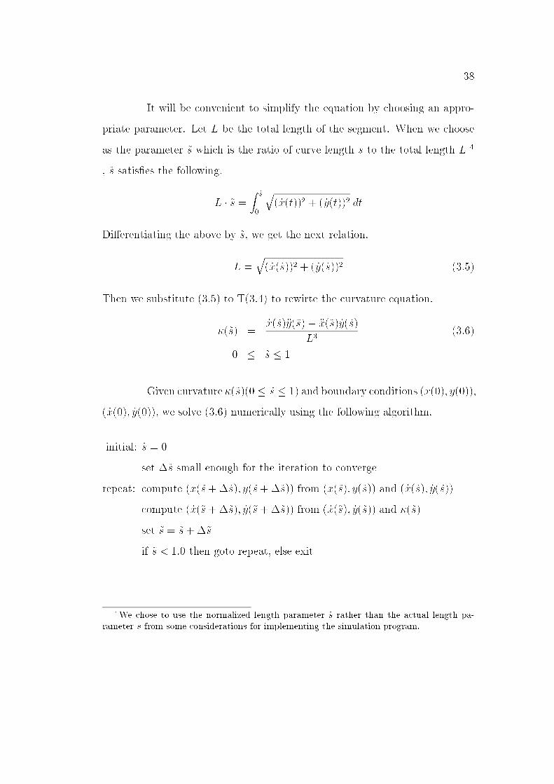
It will be convenient to simplify the equation by choosing an appro-

priate parameter. Let L be the total length of the segment. When we choose

as the parameter ~s which is the ratio of curve length s to the total length L 4

, ~s satis�es the following.

L � ~s =Z ~s

0

q( _x(t))2 + ( _y(t))2 dt

Di�erentiating the above by ~s, we get the next relation.

L =q( _x(~s))2 + ( _y(~s))2 (3:5)

Then we substitute (3.5) to T(3.4) to rewirte the curvature equation.

�(~s) =_x(~s)�y(~s)� �x(~s) _y(~s)

L3(3.6)

0 � ~s � 1

Given curvature �(~s)(0 � ~s � 1) and boundary conditions (x(0); y(0)),

( _x(0); _y(0)), we solve (3.6) numerically using the following algorithm.

initial: ~s = 0

set �~s small enough for the iteration to converge

repeat: compute (x(~s+�~s); y(~s+�~s)) from (x(~s); y(~s)) and ( _x(~s); _y(~s))

compute ( _x(~s+�~s); _y(~s+�~s)) from ( _x(~s); _y(~s)) and �(~s)

set ~s = ~s+�~s

if ~s < 1:0 then goto repeat, else exit

4We chose to use the normalized length parameter ~s rather than the actual length pa-rameter s from some considerations for implementing the simulation program.

39

It is easy to compute (x(~s+�~s); y(~s+�~s)) from (x(~s); y(~s)) and ( _x(~s); _y(~s)).

x(~s+�~s) = x(~s) + �~s � _x(~s)y(~s+�~s) = y(~s) + �~s � _y(~s)

In order to get ( _x(~s+�~s); _y(~s+�~s)), we approximate (3.6) by the following.

_x(~s) � _y(~s+�~s)� _y(~s)

�~s� _y(~s) � _x(~s+�~s)� _x(~s)

�~s= L3 � �(~s) (3:7)

We get the other equation for ( _x(~s+�~s) and _y(~s+�~s)) from (3.5).

( _x(~s+�~s))2 + ( _y(~s+�~s))2 = L2 (3:8)

By solving (3.7) and (3.8) simultaneously, we get ( _x(~s+�~s); _y(~s+�~s)) from

( _x(~s); _y(~s)). There are two algebraic solutions which satis�es (3.7) and (3.8),

and the one which is closer to ( _x(~s); _y(~s)) is what we want. The other one

corresponds to the curve with the same curvature but with an opposite orien-

tation.

Other ways to obtain a curve from curvature are by (3.2) and by

the Frenet equations (3.3). The Frenet equations give us a straightforward

expression for applying numerical integration to get curve shape from curvature

(see also Section 3.5).

3.4 Intrinsic Properties of Space Curves

For many of the notions on plane curves explained in Section 3.2,

natural extensions exist to space curves.

40

3.4.1 Regular Curve

A space curve

P(t) =

0B@ x(t)y(t)z(t)

1CA

� � t � �

is regular, if and only if the following conditions are satis�ed.

1. P(t) has continuous third derivatives in the interval de�ned.

2. _P(t), called a tangent vector, is nowhere zero.

3.4.2 Curve Length

The length of curve s(t) from a �xed point to a variable point for a

space curves is

s(t) = Lt� =

Z t

�

q_P(� ) � _P(�)d� =

Z t

�

q_x2 + _y2 + _z2d�

When we use s(t) as a parameter of the curve, the following relation holds for

a tangent vector:

j _P(s)j = 1

3.4.3 Curvature

The curvature of a space curve cannot be de�ned in the same manner

as a plane curve, and so is de�ned as follows. First, we move the starting point

of tangent vectors to the origin of the coordinate system, while we preserve

their direction. Since tangent vectors are unit vectors, the end point of the

vectors are on a unit sphere. In lieu of orientation angle �(s) used for a plane

41

curve, the length of the curve traced by the tangent vector is used to de�ne

curvature.

�(s) =Z s

s0

q_P(�) � _P(�)d�

Curvature is then de�ned by taking a derivative of the function �(s).

�(s) =d�(s)

ds=

q_P � _P

Curvature for a space curve is non-negative because of the de�nition.

3.4.4 Torsion

In 2-D, we have a special pair of unit orthogonal vectors: a tangent

vector and a normal vector. In 3-D, we have a set of three vectors. The tangent

vector v1(s) is de�ned in exactly the same manner:

v1(s) = _P(s)

For space curves, the space orthogonal to the tangent vector has two dimen-

sions. In order to single out a normal vector, we assume � > 0 or _P 6= 0 and

choose the unit vector v2(s) as:

v2(s) =_P

j _PjThe normal vector thus de�ned is orthogonal to the tangent vector, because

the tangent vector is a unit vector.

The plane determined by the two vectors is called the osculating plane.

The third vector v3(s) called the binormal vector is de�ned from the two vec-

tors:

v3(s) = v1(s)� v2(s)

42

Osculating Plane

Binormal Vector Normal Vector

Tangent Vector

Figure 3.5: Tangent, Normal, and Binormal Vectors

See Fig. 3.5.

For space curves, we have another invariant property of a curve, in

addition to curvature. Torsion � is de�ned by the next equation:

_v3 = ��v2

Note that _v3 is orthogonal to v1 and v3 and thus is parallel to v2.

3.4.5 Existence of a Space Curve given Curvature and Torsion

The Frenet equations for a space curve are:

0B@ _v1(s)

_v2(s)_v3(s)

1CA =

0B@ 0 +�(s) 0��(s) 0 +�(s)0 ��(s) 0

1CA0B@ v1(s)v2(s)v3(s)

1CA (3.9)

Using the equations, the following theorem can be shown.

43

Theorem 2 For a given continuous function �(s) > 0 and � (s) de�ned for

s0 � s � s1, there is one and only one regular curve (within a rigid motion)

such that �(s) is its curvature function, �(s) is its torsion function, and s is

its arc length.

Let us make a few comments on the assumption that �(s) > 0 in

the theorem. The Frenet equations are �rst order ordinary di�erential equa-

tions. A unique solution exists for the Frenet equations just by assuming �(s)

and � (s) are continuous, given an initial condition v1(s0), v2(s0), and v3(s0).

However, the theorem says something stronger than that, because uniqueness

of a solution as a regular curve is stated. While the assumption �(s) > 0 is

necessary for avoiding unnecessary complications in mathematics, we can view

the Frenet equations simply as a way to construct any regular curve using two

continuous functions �(s) and � (s) parameterized by its arc length.

3.5 Continuous Model in 3-D

The continuous model in 3-D is a natural extension of the continuous

model in 2-D. For each segment in the model, torsion is considered in 3-D in

addition to curvature. The torsion function is also discretized using �ve points

(sa; �a), (sb; �b), (sc; �c), (sd; �d), and (se; �e). Operators now include those to

move �a through �e. The continuous decomposition technique is extended to

3-D without di�culty.

We use the Frenet equations for space curves (3.9) to obtain a con-

�guration from curvature and torsion. We �rst apply numerical integration to

(3.9) to obtain the orthogonal vectors v1(s), v2(s), and v3(s) from curvature

�(s) and torsion �(s). Then, the space curve P(s) is obtained using the tangent

44

vector v1(s). The tangent vector was de�ned as follows.

v1(s) = _P(s)

Hence the space curve is:

P(s) = P(s0) +Z s

s0v1(�)d�

Chapter 4

Solving Open Space Problems

In the previous chapter, the continuous manipulator model was de-

�ned. In this chapter, we solve open space problems for a single segment of the

continuous model. The open space problem is to �nd a sequence of curvature

and torsion operators for a single segment to reach a goal with its tip in an un-

obstructed working environment. The open space problem can be seen as the

inverse kinematics problem (see Section 4.4.1) for a segment of the continuous

model. The result of this chapter will be extended in the next chapter, where

we de�ne four basic motion schemas to control the continuous model in both

open and cluttered space.

Section 4.1 de�nes four types of open space problems. The section also

explains the simulator which we built. Section 4.2 and 4.3 solve the open space

problems in 2-D. Related works will be reviewed in Section 4.4. The generality

of our approach, along with its 3-D extension, is discussed in Section 4.5.

4.1 Open Space Problems

4.1.1 Four Types of Open Space Problems

Table 4.1 shows the four types of open space problems which appear

according to the location of the segment in the continuous manipulator.

OSP1 naturally corresponds to the type of goals to be achieved with-

out decomposition. The rest corresponds to subgoals to be achieved by seg-

45

46

goal to achieve constraintwith base rotation without base rotation

tip position OSP1 OSP2tip position and orientation OSP3 OSP4

Table 4.1: Four Types of Open Space Problems

ments which are generated by decompositions. OSP2 corresponds to the type

of subgoals and constraints for the last segment, OSP3 for the �rst segment,

and OSP4 for intermediate segments1. Only the �rst segment is allowed to

rotate around its starting point (which is actually the base).

4.1.2 The Swan's Neck Simulator

To test our algorithms and techniques, we built a simulator on a Sym-

bolics machine and name it Swan's neck simulator after the actuator which has

inspired our research. The original simulator handles a neck of one curvature

segment and is equipped with basic hill climbing routines to solve the four

types of open space problems. Fig. 4.1 shows its simulation window. Displayed

in the simulation window are

� a sequence of con�gurations of a swan's neck.

� a sequence of curvature functions

� a trace table which shows distances to the goal, selected curvature oper-

ators, etc.

More recently, the simulator was extended to handle a series of de-

composed segments. Currently, the simulator for 2-D has been completed. The

1Segments are numbered from the base to the tip.

47

Successful Hill Climbing ********* DISTANCE-TO-GOAL *************DIST. R THETA ORIENT OPERATOR

NIL NIL NIL NIL NIL

********* DISTANCE-TO-GOAL *************DIST. R THETA ORIENT OPERATOR

NIL NIL NIL NIL NIL 0.455 -0.150 0.269 0.036 C-RIGHT

********* DISTANCE-TO-GOAL *************DIST. R THETA ORIENT OPERATOR

NIL NIL NIL NIL NIL 0.455 -0.150 0.269 0.036 C-RIGHT 0.218 -0.027 0.167-0.024 B-UP-AND-D-DOWN

********* DISTANCE-TO-GOAL *************DIST. R THETA ORIENT OPERATOR

NIL NIL NIL NIL NIL 0.455 -0.150 0.269 0.036 C-RIGHT 0.218 -0.027 0.167-0.024 B-UP-AND-D-DOWN0.172 -0.020 0.129-0.023 A-UP-AND-E-DOWN

********* DISTANCE-TO-GOAL *************DIST. R THETA ORIENT OPERATOR

NIL NIL NIL NIL NIL 0.455 -0.150 0.269 0.036 C-RIGHT 0.218 -0.027 0.167-0.024 B-UP-AND-D-DOWN0.172 -0.020 0.129-0.023 A-UP-AND-E-DOWN0.124 -0.012 0.090-0.022 A-UP-AND-E-DOWN

********* DISTANCE-TO-GOAL *************DIST. R THETA ORIENT OPERATOR

NIL NIL NIL NIL NIL 0.455 -0.150 0.269 0.036 C-RIGHT 0.218 -0.027 0.167-0.024 B-UP-AND-D-DOWN0.172 -0.020 0.129-0.023 A-UP-AND-E-DOWN0.124 -0.012 0.090-0.022 A-UP-AND-E-DOWN0.076 -0.004 0.050-0.021 A-UP-AND-E-DOWN

********* DISTANCE-TO-GOAL *************DIST. R THETA ORIENT OPERATOR

NIL NIL NIL NIL NIL 0.455 -0.150 0.269 0.036 C-RIGHT 0.218 -0.027 0.167-0.024 B-UP-AND-D-DOWN0.172 -0.020 0.129-0.023 A-UP-AND-E-DOWN0.124 -0.012 0.090-0.022 A-UP-AND-E-DOWN0.076 -0.004 0.050-0.021 A-UP-AND-E-DOWN0.051 -0.000 0.030-0.021 A-UP-AND-E-DOWN

********* DISTANCE-TO-GOAL *************DIST. R THETA ORIENT OPERATOR

NIL NIL NIL NIL NIL 0.455 -0.150 0.269 0.036 C-RIGHT 0.218 -0.027 0.167-0.024 B-UP-AND-D-DOWN0.172 -0.020 0.129-0.023 A-UP-AND-E-DOWN0.124 -0.012 0.090-0.022 A-UP-AND-E-DOWN0.076 -0.004 0.050-0.021 A-UP-AND-E-DOWN0.051 -0.000 0.030-0.021 A-UP-AND-E-DOWN0.034 0.004 0.010-0.020 A-UP-AND-E-DOWN

********* DISTANCE-TO-GOAL *************DIST. R THETA ORIENT OPERATOR

NIL NIL NIL NIL NIL 0.455 -0.150 0.269 0.036 C-RIGHT 0.218 -0.027 0.167-0.024 B-UP-AND-D-DOWN0.172 -0.020 0.129-0.023 A-UP-AND-E-DOWN0.124 -0.012 0.090-0.022 A-UP-AND-E-DOWN0.076 -0.004 0.050-0.021 A-UP-AND-E-DOWN0.051 -0.000 0.030-0.021 A-UP-AND-E-DOWN0.034 0.004 0.010-0.020 A-UP-AND-E-DOWN0.026 0.012 0.013-0.000 D-DOWN

********* DISTANCE-TO-GOAL *************DIST. R THETA ORIENT OPERATOR

NIL NIL NIL NIL NIL 0.455 -0.150 0.269 0.036 C-RIGHT 0.218 -0.027 0.167-0.024 B-UP-AND-D-DOWN0.172 -0.020 0.129-0.023 A-UP-AND-E-DOWN0.124 -0.012 0.090-0.022 A-UP-AND-E-DOWN0.076 -0.004 0.050-0.021 A-UP-AND-E-DOWN0.051 -0.000 0.030-0.021 A-UP-AND-E-DOWN0.034 0.004 0.010-0.020 A-UP-AND-E-DOWN0.026 0.012 0.013-0.000 D-DOWN 0.018 0.015 0.003 0.000 A-UP-AND-E-DOWN

Figure 4.1: Simulation Window

simulator includes a path planning module which �nds paths after a user has

speci�ed a set of obstacles. Many of the �gures in this thesis show output from

the simulator.

4.2 Hill Climbing Searches

To solve the open space problems, hill climbing searches are performed

in the following sequence.

1. set dcurr to the current distance to the goal

2. if dcurr < �, exit (the goal has been reached)

3. set �~�, magnitude of curvature operators, in proportion to dcurr

4. choose the curvature operator which makes the next distance dnext the

shortest, when applied to the current curvature function �(~s)

5. if dnext � dcurr, exit (we get caught at a local minimum)

6. update �(~s) by applying the best curvature operator

48

(curvature)(con�guration)

(e)

(d)

(c)

(b)(a)

s (e)(d)

(c)

(b)

(a)

left

down

up

right

(s)

Figure 4.2: Curvature Segment Representation and its Operators. The follow-ing curvature operators are used to change curvature (and con�guration). a. In-crease/decrease �a, �b, �c, �d, or �e (move up/down an interpolation point). b.Increase/decrease sb, sc, or sd. (move right/left an interpolation point.) c. Rotate

the base of a curve.

7. update the orientation of the base, if the base can rotate

8. goto 1, and repeat

The curvature operators de�ned in Section 3.3.1 (see also Fig. 4.2) are

used as next state functions. In order to make the magnitude of the curvature

operators independent from a curve length L, we use a normalized curvature

function ~�(~s) instead of �(~s)2.

~�(~s) = �(~s) � (L=2�)

Then the magnitude of the curvature operators is set as below based on exper-

iments.

�~� =

8><>:

0:20 if dcurr � 0:100:10 if dcurr � 0:050:05 otherwise

2Curves with ~�(~s) = �1 are circles. ~s is a normalized curve length parameter and 0 �~s � 1.

49

�~� is used as an increment/decrement of ~�(~s) when we move up/down an

interpolation point, and 0:5 � �~� is used as an increment/decrement of ~s of

~�(~s) when we move right/left an interpolation point.

Distance functions are de�ned for each type of open space problems

as follows.

dOSP1 = j�rj=LdOSP2 = j�rj=L+ j��j=�dOSP3 = j�rj=L+ j�� �� j=� + j���� j=�dOSP4 = j�rj=L+ j��j=� + j��j=�

�r = rgoal � r

�� = �goal � �

�� = �goal � �

where

L : curve length

(r; �) : polar coordinates of the tip of the current con�guration

� : orientation of the tip of the current con�guration

(rgoal; �goal) : polar coordinates of the goal position

�goal : goal orientation

� : rotation of the base, which will be explained shortly

50

r

Figure 4.3: Polar Coordinates for Distance Functions

The origin of the polar coordinate system is at the base of the neck (Fig. 4.3).

Angles are in radians. When the base is allowed to rotate, its rotation is3

� =

(�� for OSP10:5 � (�� +��) for OSP3

Fig. 4.4 shows an example of a successful hill-climbing search. This

and subsequent �gures show graphical output from our simulator. Each display

shows multiple plots of (x(s); y(s)) on the left and �(s) on the right for a �nite

sequence of times t0; : : : ; tn. The base of the arrow in the �gure represents the

goal position, and the orientation of the arrow represents the goal orientation.

4.3 Solving the Local Minima Problem

4.3.1 The Local Minima Problem

OSP1 is easy, because OSP1 has no local minima. All the others have

local minima. But the local minima problem is most evident in OSP4 where

achieving rgoal,�goal, and �goal can compete with one another. Hence, we will

3Rotation is chosen to make the distance the shortest.

51

0 1

23

Figure 4.4: Successful Hill-Climbing

0

1

2 34

Figure 4.5: Local Minimum in Hill Climbing

talk about OSP4 from now on. Fig. 4.5 is a typical example of getting caught in

a local minimum. The naive hill climbing search works in Fig. 4.4 but doesn't

in Fig. 4.5.

Besides the local minima problem, the type of the hill climbing search

shown in Fig. 4.5 is not good because it usually leads to solutions with con�g-

urations which are either self-intersecting or have large curvature. We prefer

con�gurations with small curvature, because they will be easier to approximate

52

by a jointed arm.

Changing the distance functions, for instance , putting more weight

on �� in dOSP4 to emphasize an orientation, sometimes works, but tends to

make another local minimum. We could get rid of some local minima by using

coordinated operators built on top of the original curvature operators. For

example increasing �b and decreasing �d at the same time in Fig. 4.2 is e�ective

in decreasing the radius r without changing the tip orientation � much, because

� �� �04 is proportional to

R 10 �(~s)d~s.

� r is inversely proportional toR 10 j�(~s)jd~s.

We can thus get a new curvature operator to attain competing goals simulta-

neously. But in general, coordinated operators are more e�ective for the �ne

tuning of con�gurations rather than for solving the local minima problem. We

still have local minima.

4.3.2 Typical Con�gurations

Let's go back to the examples in Fig. 4.4 and 4.5. Why does the hill

climbing search work in one of them and not in the other? In a sense, it is

obvious. In the �rst example, the initial con�guration is qualitatively similar

to the �nal con�guration. On the other hand, the initial con�guration and the

goal con�guration are qualitatively di�erent in the second example. We can

envision the successful �nal con�guration for the second example as an arc-like

one with no in ection point.

4�0 is the base orientation.

53

type 4type 3type 2type 1type 0

Figure 4.6: Curvature Segment Type

On the basis of the above observation, we tried to coarsely classify

the in�nitely many con�gurations by picking up several typical con�gurations.

The typical con�gurations have been chosen according to the sign(s) of their

curvature function. If we limit the number of in ection points within a segment

to one, we have only �ve curvature segment types (Fig. 4.6).

In the hill climbing search, given �, �, and r in Fig. 4.3 are to be

achieved. Let us �x the base orientation �0 to some arbitrary value, say 180�,

and consider � and � ignoring r. The con�gurations of the �ve curvature

segment types occupies �ve distinctive places in �-� plane. See Fig. 4.7. For

any point in the �-� plane, there is a segment type in its neighborhood.

4.3.3 Interpolation to a Good Initial Con�guration

We added a capability of �nding a good initial con�guration for hill-

climbing searches. We stored in the simulator �ve typical con�gurations which

represent the �ve curvature segment types5. The maximum of ~�(~s) for these

con�gurations are set to �1.

Prior to a hill climbing search, the simulator searches the stored con-

�gurations for the best initial con�guration. The best con�guration is the one

5Their curvature along with r,�, and � are stored.

54

type-3type-4

type-0 type-0

type-4 type-3

type-2type-1

-180

-90

180

90

-180 -90 180900

Figure 4.7: Curvature Segment Types in �-� Plane

which is the closest to the goal in terms of the distance functions which were de-

�ned for the hill climbing search, after the stored con�gurations are scaled and

rotated so that they have the same length and base orientation as the segment

being simulated (see Fig. 4.8). Here, we need to have a precompiled movement

routine to move from the actual initial con�guration to the one suitable for hill

climbing. Since we know the curvature pro�le of both con�gurations, this can

be done easily. In order to move from one con�guation to another, we sim-

ply interpolate the corresponding curvature parameters for the two curvature

pro�les to obtain the intermediate curvature pro�les and the con�gurations.

Fig. 4.9 shows a solution of the same example in Fig. 4.5.

55

Figure 4.8: Five Candidate Initial Con�gurations

0

1

2

8

9

10

0

1

23

4 5

Figure 4.9: Interpolate to Good Initial Con�guration and Hill Climbing

56

4.3.4 Simulation Results

The initial con�guration �nding capability has turned out to be very

e�ective. We were afraid that we might need lots of con�gurations as candi-

dates, but it was not necessary. Judging from our experiments, it seems that

the �ve con�gurations (and a few more at most) are su�cient as far as open

space problems are concerned. The simulator sometimes gets caught in local

minima, but it happens only when the neck is very close to the goal. We be-

lieve this situation can be improved by adding a few coordinated motions or by

�ne tuning �~�. We attach at the end of this chapter some of the open space

problems solved.

4.4 Related Work on Inverse Kinematics

The open space problem we have solved can be seen as inverse kine-

matics for a single segment of the continuous model. In this section, we review

some of the methods for inverse kinematics developed for redundant manipu-

lators, �rst for redundant jointed arms and then for continuous arms.

4.4.1 Redundant Jointed Arms

The inverse kinematics problem is de�ned as follows. Let q be a

vector of joint coordinates, and x be a vector of end e�ector coordinates. Then

forward kinematics is a mapping f from q to x:

x = f(q) (4:1)

The inverse kinematics is to �nd the inverse of f :

q = f�1(x) (4:2)

57

For redundant manipulators, inverse kinematics have an in�nite num-

ber of solutions. An optimization procedure can be used to choose the set of

solutions subject to an objective function. Closed form solutions are di�cult

to obtain for such cases, and most of the research on the problem has been

based on a di�erential representation of (4.1) and (4.2):

_x = J(q) _q (4.3)

_q = J�1(q) _x (4.4)

where J�1(q) is a generalized inverse of the Jacobian matrix J , which can be

uniquely determined by taking into account a speci�ed objective function. (4.4)

is used iteratively to move the end e�ector to its goal. The techniques which we

discussed in Section 1.4 are examples of this approach, where objective func-

tions are chosen so as to avoid obstacles. [Goldenberg et al. 85] generalized

these techniques. They reformulated the inverse kinematics problem for redun-

dant manipulators as a constrained nonlinear optimization problem, and used

a modi�ed Newton-Raphson method to solve a set of nonlinear equations.

Applying arti�cial neural network techniques to learning inverse kine-

matics or inverse di�erential kinematics has been tried [Josin 88, Ackley 89,

Mel 90, Barhen et al. 89, Yeung and Gekey 89], and many of these approaches

deal with redundant manipulators. [Mel 90] deals with a 3 DOF planar manip-

ulator, [Ackley 89] with a 5 DOF planar manipulator, [Barhen et al. 89] with

manipulators with many degrees of freedom. One of the advantages of these

techniques over numerical optimization techniques would be e�ciency, i.e. a

rapid convergence to a solution after the network has learned from examples

the non-linear transformation J�1(q).

58

4.4.2 Continuous Arms

Kinematics of continuous arms has attracted little attention. Repre-

senting highly redundant manipulators with a continuous model is itself a quite

distinctive approach.

In an attempt to �nd a good initial con�guration for his digital ma-

nipulator, [Pieper 68] developed an algorithm to �nd a curve which is made up

of four connected circular arcs in such a way that they have the same radius,

and adjacent arcs have the same tangent. The coordinates and the orientation

of the tip along with the length of the curve is speci�ed. By expressing the

constraints using trigonometric equations, the curve which satis�es the require-

ments can be found.

[Chirikjian and Burdick 90] presents an approach similar to ours. The

authors also represent highly redundant manipulators using a continuous ma-

nipulator model. While we use spline interpolation to discretize curvature and

torsion, they use modal decompositions. For example, the curvature function

can be represented as :

�(s) =NXi=1

ai�i(s) (4.5)

where �i(s)'s are called modes, and ai's participation factors. In particular, for

the primary mode of curvature functions:

�(s) = acos(2�s) + bsin(2�s) (4:6)

they have derived a closed form solution to the inverse kinematics problem:

(x; y) 7! (a; b) (4:7)

by using the following formula:

�(s) = �(s0) +Z s

s0�(�)d�

59

P(s) =

x(s0) +

R ss0cos �(�)d�

y(s0) +R ss0sin �(�)d�

!

The formula was introduced in Section 3.2 as (3.2). However, limiting curvature

functions to the form (4.6) is too restrictive. Moreover, no equation exists for

space curves which is equivalent to (3.2). This implies that in general we have

to rely on numerical techniques in lieu of closed form solutions.

4.4.3 Research on Curve Design

Somewhat related research, the study of curves which satisfy certain

conditions, has been done in computer graphics and applied mathematics.

There is a body of research on designing curves from curvature and

torsion, their intrinsic properties [Nutbourne et al. 72, Pal and Nutbourne 77,

Pal 78a, Pal 78b, Schechter 78a, Schechter 78b]. This research is motivated by

the fact that it is often the case that design engineers want to specify the shape

of curves in terms of their intrinsic properties, rather than interpolation points

or control vertices. For example, piecewise linear curvature functions are used

to design plane curves in [Nutbourne et al. 72]. [Pal 78a] presents an algorithm

to generate a curvature continuous space curve through two points with given

tangent directions. Their approach to designing curves through curvature cer-

tainly has some appeal to us. But further investigation is necessary in order to

extend their technique to the inverse kinematics problem, because curve length

cannot generally be speci�ed.

Also interesting is the research on constructing curves which are par-

ticularly smooth [Horn 83, Kallay 87, Jou and Han 90]. When the ends of a

thin elastic beam are clamped, it will assume a shape which minimizes the

60

elastic energy:

E =Z L

0�2ds (4:8)

Curves which satisfy (4.8) are called minimum energy splines. The problem

of �nding a minimum energy spline given its boundary conditions can be seen

as a variation of the open space problems. It has been suggested that humans

use this class of curves when they try to complete a partially speci�ed contour

map [Horn 83]. [Jou and Han 90] discusses the planar problem, where we have

angle constraints at both ends, and a prescribed length for the spline curve. The

existence of such splines when the distance between the two end points is within

prescribed length is proved, and an iterative algorithm to solve the constraint

minimization problem is presented. [Kallay 87] presents an algorithm for the

same problem in 3-D.

4.5 Summary of the Chapter

In Section 4.2 and 4.3, we have solved the open space problems in

2-D. In the previous section, we have seen many other methods for inverse

kinematics for redundant manipulators. We notice a similarity of these methods

to our method. No matter whether the method is intended for jointed arms

or for continuous arms, similar procedures are used either in the space of joint

variables or in the space of curvature parameters.

We believe that we must resort to an iterative procedure to solve the

open space / inverse kinematics problems for highly redundant manipulators.

Closed form solutions cannot be obtained except for a very limited class of

problems. Possible iterative techniques include a modi�ed Newton-Raphson

method or hill climbing search which we use. Learning using neural networks

can also classi�ed in this category of techniques.

61

One advantage of the modi�ed Newton-Raphson method is that an

optimality criterion can be incorporated in determining a generalized inverse of

the Jacobian matrix through optimization in n� 6 dimensional space for an n

DOF manipulator. However, the method cannot be applied to continuous arms

because its Jacobian matrix cannot explicitly be obtained. On the other hand,

hill climbing search can be applied to the continuous manipulator model, and

our hill climbing search is still in an 8-D space (the space of curvature operators)

for a single segment. Furthermore, path planning will become much easier by

using the continuous model, as we will see in the following chapters. The local

minima problem is inherent to both of the techniques, and starting from an

initial value close to the solution is necessary in order not to be caught at local

minima. We have also addressed the problem of �nding a good initial value for

our hill climbing search.

While the techniques we have developed are for solving 2-D problems,

3-D problems can be solved by extending the techniques in a straightforward

fashion. It will be easy to extend our hill climbing search so that torsion

parameters are also be changed to reach a goal in 3-D space. The local minima

problem for the extended hill-climbing search will be dealt with in the same

way, by storing typical con�gurations as candidate initial states for the search.

Experiments in 3-D are necessary to �nd a set of typical con�gurations adequate

to avoid local minima.

62

Figure 4.10: Example 1 as OSP1

Figure 4.11: Example 1 as OSP2

Figure 4.12: Example 1 as OSP3

Figure 4.13: Example 1 as OSP4

63

Figure 4.14: Example 2 as OSP4

Figure 4.15: Example 3 as OSP4

Chapter 5

Basic Motion Schemas for Path Planning

In the open space problems discussed in the previous chapter, we

are concerned only about the tip position/orientation to reach a goal, hence

we need only one segment. To solve a more complex problem, the manipulator

can be segmented at points along the length of the manipulator, and individual

motion schemas are combined to achieve multiple subgoals along its length.

In this chapter, we de�ne basic motion schemas that control an in-

dividual segment of the continuous manipulator. We express a motion plan

for the continuous manipulator using decompositions and motion schemas. By

executing the plan, the manipulator trajectory will be obtained. The path

planning problem for the continuous manipulator model is analyzed, and our

approach to the problem is introduced.

5.1 The Basic Motion Schemas

We de�ne four basic motion schemas that control an individual seg-

ment:

Hill-climb: Hill climb to achieve tip position and/or orientation or end cur-

vature/torsion.

Interpolate: Move by interpolation between two speci�ed curvature/torsion

pro�les.

64

65

Feed/Retract: Increase (decrease) the length allocated to a segment by mov-

ing the tip along a trajectory to reach a given position/orientation.

Fold/Unfold: Increase (decrease) the length allocated to a segment, while

maintaining tip position and orientation.

The �rst two motion schemas are de�ned to solve the open space problems.

The other are added to control a segment in cluttered space. Using the decom-

position technique, the motion schemas can be combined to control the whole

manipulator. Details follow on each motion schema we have implemented for

the 2-D simulation.

5.1.1 Motion Schemas for Open Space

A Hill-climb schema executes a set of hill-climbing routines to achieve

the four types of open space problems. Distance functions for hill climbing

search are de�ned based on the goal, the tip and the rotation of the base. The

curvature operators are used as next-state functions with magnitude scaled in

proportion to the current distance to the goal. To have continuous curvature

in decompositions, another hill climbing routine has been added to achieve end

curvature while maintaining its tip position and orientation.

An Interpolate schema moves by interpolation between two speci�ed

curvature pro�les. Each of the curvature parameters, (sa; �a), (sb; �b), (sc; �c),

(sd; �d), and (se; �e), is linearly interpolated.

sinterpolated�

= (1� p)sfrom�

+ psto�

�interpolated�

= (1� p)�from�

+ p�to�

where p moves from 0:0 to 1:0. The naive hill climbing search does not always

work, because it may get caught at a local minimum. Hill climbing search works

66

(1) (2) (3)

Figure 5.1: Feed/Retract Motion Schemas

when it starts from a con�guration close to the �nal con�guration. Hence,

we select and move to a good initial con�guration before hill-climbing search.

Interpolate motion schema moves from the actual initial con�guration to the

selected con�guration.

5.1.2 Motion Schemas for Cluttered Space

Feed/Retract motion schemas increase (decrease) the length allocated

to a segment by moving the tip along a trajectory to reach a given posi-

tion/orientation (Fig. 5.1). This is a motion schema to represent the follow-

the-leader type, snake-like motion considered in [Clement and I~nigo 90] which

was introduced in Section 1.2. The trajectory is selected from those which

correspond to the �ve typical con�gurations and cubic spiral curves (see Chap-

ter 6). Since the con�guration (shape) of a segment is controlled by �ve points

to represent curvature, the curvature pro�le of the speci�ed trajectory is traced

(by the �ve points) rather than the trajectory itself. The trajectory determines

how precisely we can feed or retract a segment along the trajectory.

Fold/Unfold motion schemas increase (decrease) the length allocated

to a segment, while maintaining tip position and orientation (Fig. 5.2). This

motion schema is implemented as another kind of hill climbing search. The

length for the segment is increased (decreased) incrementally step by step.

67

For each step, we perform a hill climbing search to maintain the tip posi-

tion/orientation.

Figure 5.2: Fold/Unfold Motion Schemas

5.2 Using Motion Schemas with Decomposition

Amotion plan is expressed using the basic motion schemas. Figure 5.3

shows the structure of a plan. The solution to the local minima problem in

open space (�gure 4.9) uses two motion schemas, Interpolate and Hill-climb,

after selecting an appropriate curvature segment type. The manipulator can

be decomposed to achieve multiple subgoals along the length of the continu-

ous manipulator. Each subgoal is then achieved by executing motion schemas

for the corresponding segment. Four decompositions have been implemented:

add/delete a segment, divide a segment at a speci�ed point, and merge two

..... iSTEPSTEP

.....

PLAN

1 STEP n

SCHEMA SCHEMA

Figure 5.3: Motion Plan Representation

68

neighboring segments.

The motion plan is then executed to obtain a trajectory. Use of the

motion schemas with decompositions is demonstrated in �gure 5.4, where we

fold, rotate, and extend the manipulator.

To achieve a set of subgoals along the length of the manipulator,

Frames 7-10 in Fig. 5.4 are repeated:

For each of the subgoals, the following steps are executed.

1. Add a segment at the tip of the continuous manipulator. The initial

length of the added segment is zero.

2. Feed the new segment incrementally while unfolding the segment of the

manipulator near the base by the same increment of length. Please refer

to Fig. 5.4 on the details of the motion schemas used to unfold the ma-

nipulator.

The next two steps are necessary, because the curvature pro�le of the

path segment is approximated using the �ve points.

3. Hill climb for the tip segment to achieve the subgoal position precisely.

4. Hill climb to set end curvature to zero while maintaining the subgoal

position.

5.3 Path Planning Problem for the Continuous Manip-

ulator

We have solved the open space problem. We have also demonstrated

the use of decompositions and motion schemas. Now let us combine these

results and attack the whole problem: given a highly redundant manipulator

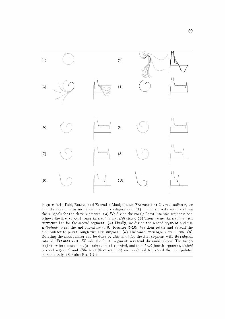
69

(1) (2)

(3) (4)

(5) (6)

(7) (8)

(9) (10)

Figure 5.4: Fold, Rotate, and Extend a Manipulator: Frames 1-4: Given a radius r, wefold the manipulator into a circular arc con�guration. (1) The circle with vectors showsthe subgoals for the three segments. (2) We divide the manipulator into two segments andachieve the �rst subgoal using Interpolate and Hill-climb. (3) Then we use Interpolate withcurvature 1=r for the second segment. (4) Finally, we divide the second segment and useHill-climb to set the end curvature to 0. Frames 5-10: We then rotate and extend themanipulator to pass through two new subgoals. (5) The two new subgoals are shown. (6)Rotating the manipulator can be done by Hill-climb for the �rst segment with its subgoalrotated. Frames 7-10: We add the fourth segment to extend the manipulator. The targettrajectory for the segment (a straight line) is selected, and then Feed (fourth segment), Unfold

(second segment) and Hill-climb (�rst segment) are combined to extend the manipulatorincrementally. (See also Fig. 7.2.)

70

and its environment, how can we �nd a collision free trajectory automatically

and e�ciently?. Figure 5.5 is an overview of a motion planning system and the

area enclosed by dotted lines are what we have explained so far. The dynamic

simulation is explained in [Park 90].

5.3.1 Where Do We Start?

The following proposition shows where we start.

Proposition 1 Suppose we have a continuous curvature manipulator with vari-

able length. Then, given polygonal obstacles, we can �nd a collision free path

from a current con�guration to the goal con�guration. The time complexity is

polynomial in the number of obstacle corners.

Proof (sketch). First, we �nd a con�guration to reach the goal from the base.

For a point robot, there is an e�cient algorithm called visibility graph method to

�nd the shortest path in 2-D space which is cluttered with polygonal obstacles.

A visibility graph is constructed by making both obstacle corners and start/end

points nodes of the graph and by connecting those nodes which are visible from

each other. The shortest path can be found by searching through the visibility

graph. See [Sharir and Schorr 84] for a sketch of the method. The problem can

be solved in O(n2 log n) time where n is the number of obstacle corners. The

algorithm has been improved to O(n2) time [Asano 85, Welzl 85].

Then it is easy to transform the polygonal path to a one which is also

collision free and has smooth corners (has curvature continuity). We can apply

the method in [Kanayama and Hartman 89] which uses cubic spiral curves for

71

collision free trajectory

evaluationmapping error

subgoals

currentcon�guration goal

Dynamic Simulation

Jointed armtrajectory

schemas

Open Space Problem

(four variations)

Continuous Manipulator

hill-climbing curvature types

free convex regions

decomposition

path planning

obstacles

Figure 5.5: Overview of the Motion Planning System: the area enclosed with dotted

lines has been explained so far.

72

STARTGOAL

Figure 5.6: Visibility Graph Method To Find a Polygonal Path. Obstacles bound-aries are drawn in dotted lines and are grown to make room for turns.

turns to maintain curvature continuity1. By growing the obstacles a little in

advance, we can �nd enough space to make small smooth turns.

We are going to retract the manipulator to a point at the base, and

then extend the manipulator to the goal along the continuous curvature path

found. A little bit care must be taken, because our continuous curvature ma-

nipulator model is controlled by the curvature parameters, and hence cannot

precisely follow the curvature pro�le of the path found. To obtain the curvature

pro�le for the continuous manipulator, we use motion schemas.

We assign a unit cost to each motion schema execution. The unit cost

assignment is justi�ed because the task here is considered to be a control task,

rather than a planning task as follows.

� The unit cost does not include the cost for planning. A continuous cur-

vature path for a point robot has already been found, consisting of cubic

spiral segments.

1Cubic spiral curves will be explained in the next chapter.

73

� The objective for each motion schema execution is to trace each of the

above cubic spiral segments with a single segment of the continuous

model.

� The curvature pro�le of a cubic spiral curve is a quadratic function of

length s, simple enough to be traced (interpolated) by a single segment

of the continuous model with its �ve curvature parameters adjusted. In

fact, iterations for adjusting curvature parameters converge rapidly.

We �rst retract the whole length of the manipulator and make it a

point at the base. If the current con�guration has m curvature segments, this

takes O(m) steps using decompositions and schemas.

Following the above smooth path is just a reverse process of retracting

the whole manipulator. Since the shortest path between two given points must

be a polygonal line whose vertices are corners of obstacles, the total number of

the straight line segments of the path is O(n). We need one curvature segment

for each turn. Then the total number of curvature segments we need is O(n),

including those for turns. This also shows that we can assume m = O(n). 2

5.3.2 Remaining Problems

The previous proposition is important because it shows that the al-

gorithm is dependent on the complexity of the environment rather than the

degree of freedom of the manipulator, thanks to the continuous manipulator

model. The property comes from the ability of the continuous manipulator to

follow its tip trajectory.

But it is not a complete solution, because we are neglecting the fol-

lowing considerations.

74

[Manipulator Length] Manipulators have �xed length.

[Trajectory Finding] This is a problem of changing from a current con�g-

uration to a �nal con�guration without colliding obstacles. Retracting

the whole and reaching from the base is not possible for �xed length

manipulators.

[Maximum Curvature] In the proposition, we did not put any limitation on

curvature values. Kokkinis and Wilson studied the hardware architec-

tures of continuous robotic arms in [Kokkinis and Wilson 88], and found

that the maximum curvature is one of the most important performance

measures. We need to �nd a smooth path whose curvature does not

exceed a given maximum value.

[Evaluating Errors of Mapping to a Jointed Arm] Intuitively, con�gura-

tions (curves) with large curvature are more di�cult to approximate using

a jointed arm. We need to evaluate the upper bound of the mapping er-

rors, given a jointed arm and the maximum curvature. Then, we can

"grow obstacles" by an appropriate amount in advance so that a collision

free con�guration for the continuous manipulator within the maximum

curvature is guaranteed to be mapped to a collision free con�guration for

a jointed arm (see Fig. 5.7).

5.3.3 Our Approach

The �rst two problems are di�cult. As to the manipulator length

control, think of this. There are e�cient algorithms to �nd the shortest path

or nearly the shortest path in 2D. But �nding a path with the desired length

seems to be much harder. For example, a somewhat similar discrete problem:

75

J0

J1

J2J3

J4J5

J6

J7J8

Figure 5.7: Grow Obstacles

the longest path problem for a weighted graph is proved to be NP complete

[Garey and Johnson 79].

In order to turn around the problems, we assume some open space

around the base to fold/unfold the manipulator. With the assumption, the

length is controled by folding/unfolding the manipulator, and the trajectory

can be found simply by retracting/extending the manipulator. We present an

algorithm to �nd a path with maximum curvature constraint in Chapter 6,7.

In Chapter 8, we show how to set the maximum curvature constraint, given a

jointed arm.

Chapter 6

Planning a Smooth Path for Autonomous Vehicles

using Primary Convex Regions

This chapter is about path planning for autonomous vehicles. It is

included, because the algorithm to �nd smooth paths for autonomous vehicles

can be directly applied to path planning for the continuous manipulator model.

This is a self contained chapter. First, the problem of �nding smooth

paths is introduced. Then, we present an algorithm to �nd smooth paths. Our

algorithm is based on decomposing free space into primary convex regions, and

is a natural extention of previous algorithms which �nd straight line paths.

6.1 Introduction

Smoothness of path is critical for autonomous vehicle navigation.

Trying to follow unsmooth paths leads to "stop,turn, and move" or "back-

ing up maneuver" strategies. There are algorithms to �nd a path which con-

sists of straight line and tangent circular arc segments [Wilfong 88, Wilfong 89,

Jacobs and Canny 89, Basu and Aloimonos 90]. However, curvature disconti-

nuity exists at every tangent point in these paths, because circular arcs have

constant curvature equal to the inverse of their radius and straight lines have

zero curvature. This type of path is criticized for not being smooth enough for

autonomous vehicles to follow easily [Kanayama and Hartman 89, Nelson 89].

For example, spline curves are recommended over circular arcs for highway

transition curves [Barnett 38].

76

77

[Kanayama and Hartman 89] proposes using cubic spiral curves to

make a smooth (i.e. continuous curvature) move from one position and orien-

tation to another. Cubic spirals can be constructed to have zero curvature at

tangent points. But they did not address the path planning problem.

We present a path planning algorithm to �nd a smooth path which

consists of straight lines and cubic spirals. The maximum curvature of cubic

spirals is restricted to allow for the vehicle's constraints. Our algorithm is based

on decomposing free space into primary convex regions [Rueb and Wong 87,

Singh and Wagh 87]. We naturally extend previous algorithms which �nd

straight line paths. Overlapping regions of the primary convex regions are

used to make smooth turns from one region to another. Large overlapping

regions can be further divided in order not to miss smooth turns. Because

of the convex nature of free regions, we can adjust the places of turns easily

while keeping a path within free space. We �nd the shortest smooth path using

standard graph search techniques for the connectivity graph which is built on

top of the representation.

The rest of the chapter is organized as follows. Section 6.2 concerns

free space decomposition into convex regions. Conditions for making a smooth

turn between regions are made explicit in section 6.3. Section 6.4 discusses

building a connectivity graph of regions and the search for a smooth path.

6.2 Free Space Decomposition

We assume obstacles are given as a set of polygons. We �rst decom-

pose free space into convex regions using existing methods in literature. It is

claimed that path planning algorithms using free space decomposition are bet-

ter suited for navigation purposes than con�guration space algorithms, because

78

free convex regions can be used to locate and guide the robot locally within

the regions by measuring its distance to the region edges1. This eliminates the

requirement for an accurate global coordinate system to track the position of

the robot in navigation. [Rueb and Wong 87].

6.2.1 Free Space Decomposition Methods

We need to select a primitive for free space decomposition best suited

to our task: �nding smooth paths.

[Brooks 83a] is one of the earliest papers on free space decomposition

for path planning. In his algorithm, free space is decomposed into generalized

cones which are considered to be free ways. But the robot is required to pass

along the spines of generalized cones, which leaves less room for our path op-

timization algorithm to make smooth turns. Moreover, since generalized cones

are not convex regions in a strict sense, it follows that if we change the position

of a corner within an intersection of two cones, the located line segment is not

guaranteed to be within the cone.

[Kuan et al. 85] decomposes free space into two sets of disjoint poly-

gons: passage regions and channel regions. Passage regions correspond to open

space (rooms, squares,..), and channel regions to paths connecting open space.

Passage regions may be good candidates for smooth turns. However, a large

open space does not necessarily become a passage region, because passage re-

gions and channel regions are determined only from the topology of obstacle

layout without considering the size of areas. Moreover, since this algorithm de-

1This does not apply to all the free space decomposition methods. Only those decompo-sition methods to convex regions whose edges correspond to actual walls have this property.

79

(1) (2) (3)

Figure 6.1: Wall Segments and Primary Convex Regions. (1) Obstacles and bound-

aries. (2)Wall segments are shown as line segments. (3) Each primary convex regionis shrinked for visibility.

composes free space into disjoint convex regions, it does not recognize straight

line path segments if they exist, so that the path obtained will have more line

segments (and more turns) than paths obtained by other methods.

6.2.2 Primary Convex Regions

[Singh and Wagh 87, Rueb and Wong 87] use primary convex regions

as a primitive to represent free space, in order to �nd polygonal paths. A pri-

mary convex region (PCR) is an unobstructed convex region with each bound-

ary edge covering some portion of an obstacle wall (See �gure 6.1).

Since each edge of a primary convex region covers some portion of an

obstacle wall, the region seems to be a natural description of the open space

bounded by obstacles. In addition, PCR can be seen as an extension of the

passage regions described in [Kuan et al. 85]. In fact, for any passage region,

there exists some primary convex region which contains the passage region.

PCRs are suitable representation for our task for the following reasons:

� PCRs are maximal (in area) convex regions surrounded by obstacle edges.

80

� The convexity of PCRs makes the path optimization easier. If we change

the position of a corner within the intersection of two PCRs, the moved

line segments are guaranteed to be still within the two PCRs.

� The intersections of PCRs are also convex regions, which is a desirable

property.

� Since free space is decomposed into intersecting PCRs, it is easier to �nd

a straight line path segment, and hence obtain paths with fewer turns.

Use of primary convex regions to represent free space has renewed much at-

tention recently. An algorithm to detect primary convex regions from an input

image was presented in [Tokuta and Hughes 90]. [Habib and Yuta 89] exper-

imented with Singh and Wagh's method using an actual mobile robot and

reported good results.

6.2.3 Hypergraph Method for Finding PCRs

We have implemented the algorithm in [Rueb and Wong 87] to �nd

PCRs given obstacles. PCRs are found by a directed search for a set of fun-

damental circuits in an abstract graphical representation of the environment

geometry. The nodes in the graph are wall segments obtained by extending

obstacle walls (see Fig. 6.1).

Let n be the total number of obstacle walls. The total number of

wall segments is then O(n2). Rueb and Wong's algorithm to �nd fundamental

circuits in a graph runs in time proportional to the square of the number of

nodes in the graph. Hence the complexity of their algorithm is O(n4). We can

also obtain an upper bound for the total number of primary convex regions:

O(n4).

81

PCR

PCR center of gravity

2

1

Figure 6.2: Candidate Turning Corners

Although the worst case complexity of the algorithm is not favorable,

the algorithm is e�cient in practice. Rueb and Wong reported an O(n) perfor-

mance result (compared to O(n4) for the worst case analysis). This is because

in reasonable environments the total number of wall segments is linear in the

number of wall edges; and because their algorithm to �nd fundamental cir-

cuits usually runs in linear time (in the number of nodes) by employing some

heuristics.

6.3 Making a Smooth Turn between PCRs

6.3.1 Candidate Turning Corners

Finding a polygonal path is easy, once PCRs are obtained. To move

from one PCR to another PCR, a turn can be made anywhere within the

intersection of two PCRs.

However, in order to make a smooth turn from one PCR to another

PCR while satisfying the maximum curvature constraint, we need to locate

turning corners appropriately. This is necessary also for �nding a shorter path

to reach a goal. For a small overlapping region, we use its center of gravity as

a turning corner. A large overlapping region can be further divided around its

center of gravity in order not miss smooth turns. See �gure 6.2. Due to the

82

Figure 6.3: Cubic Spirals and Circles: Curves outside are tangent circles, whilethose inside are cubic spirals (in left �gures). While circles have constant curvature,cubic spirals have quadratic curvature functions (in right �gures).

convexity of PCRs, the line segments are guaranteed to be within the PCRs.

6.3.2 Cubic Spirals

We use cubic spirals to provide a continuous curvature path, since

they can be constructed to have zero curvature at tangent points. A cubic

spiral is a curve whose orientation (integration of the curvature) is described

by a cubic function of path distance s. See �gure 6.3 to see the di�erence

between cubic spirals and circles.

Other spline curves such as Bezier curves or B-spline curves (see

[Farin 90]) share some of the favorable properties of cubic spiral curves. Bezier

curves and B-spline curves have the convex hull property which makes it possi-

ble to �t generated curves within free space by choosing control vertices appro-

priately. They can be constructed to have zero curvature at end points, too.

However, the following properties of cubic spiral curves make them especially

suitable for the mobile robot navigation problem.

83

� Cubic spiral curves are particularly smooth in the sense that they mini-

mize the following cost [Kanayama and Hartman 89].

Z l

0( _�(s))2ds

The cost represents the variation of the instantaneous centripetal accel-

eration (or jerk), because the acceleration is proportional to curvature.

� Maximum curvature is more easily controlled for cubic spiral curves than

other spline curves because of their resemblance to circular arcs (see

Fig. 6.3). It has been proved that the shortest path in 2-D with a maxi-

mum curvature constraint (without the curvature continuity requirement)

consists of circular arcs and straight lines [Dubins 57].

6.3.3 Making Smooth Turns using Cubic Spiral Curves

[Kanayama and Hartman 89] presents a method to make a smooth

move from one position and orientation to another, using cubic spiral curves .

Proposition 2 (Kanayama and Hartman) If the size d and the de ection

� of a cubic spiral is given (�gure 6.4), its length l, curvature � are

l =d

D(�)(6.1)

�(s) =6�D(�)3

d3((l

2)2 � s2) (6.2)

where

s 2 [� l2;+

l

2]

D(�) = 2Z 1=2

0cos(�(3=2� 2s2)s)ds

84

d

cubic spiral

Figure 6.4: Making a Smooth Turn using a Cubic Spiral

This result is directly applicable to making a smooth turn. For each

candidate corner, we check whether we can make a turn as follows.

1. Find dmin, the minimum d consistent with the maximum curvature con-

straint.

2. Find dfreemax, the maximum d for which the curve lies entirely within free

space.

3. Find dfitmax, the maximum d for a cubic spiral to �t along both tangent

line segments.

4. Check dmin � min(dfreemax; dfitmax). This guarantees that we can make a

collision free turn within the maximum curvature.

In order to �nd dmin, note that �(s) in (6.2) has its maximum at the

midpoint:

�max = �(0) =1:5�D(�)

d(6.3)

Therefore,

d � dmin =1:5�D(�)

�max(6.4)

85

cubic spiralfreemaxd

�tmaxd

2l

1l

Figure 6.5: dfreemax and dfitmax

To �nd dfreemax is not easy, because cubic spirals are expressed via cur-

vature. However, a cubic spiral is always contained in the area outlined by its

tangent lines and the circular arc which is tangent at the same points. Such

circles are shown in �gure 6.3 with cubic spirals. To �nd a tangent arc which

is both collision free and has the maximal radius rmax, we apply the condi-

tion that the arc passes through one of the corners of the overlapping region

(�gure 6.5), and obtain:

d � dfreemax = 2rmaxsin(�=2) (6.5)

It is possible to �nd whether we can �t smooth turns by using dmin

and dfreemax obtained, given a whole candidate polygonal path. However, this leads

to an exhaustive search, because each turn a�ects the preceding and following

turns. To avoid an exhaustive search, we use a local �t method. When making

a turn, we con�ne its starting/ending point to within a distance of lmin =

min(l1=2; l2=2) from the turning corner, where l1 (l2) is the length of a incoming

(outgoing) line segment (�gure 6.5). To make a turn within lmin, d must satisfy

the following:

d � dfitmax = 2lmincos(�=2) (6.6)

86

6.4 Graph Search for a Smooth Path

The previous section explained a method to determine whether a

vehicle can move from one PCR to another by making a smooth turn, i.e.

the connectivity between two PCRs. We then build a connectivity graph and

search for a path which satis�es the maximum curvature constraint.

6.4.1 Connectivity Graph

Nodes in the connectivity graph represent the straight line segments

within PCRs. An end point of such a line segment is either a candidate corner

inside an overlap with another PCR or the initial or goal position of a point

robot. An edge from a node Ni to Nj exists if and only if the corresponding

line segments Li and Lj share an end point and there is a smooth turn from Li

to Lj as explained in Section 6.3. The cost (length) of the edge is the length

of the partial path (a cubic spiral or a line segment)

1. from the start point of Li to the midpoint of Lj , if the start point of Li

is the initial position,

2. from the mid point of Li to the end point of Lj, if the end point of Lj is

the goal position,

3. from the midpoint of Li to the midpoint of Lj , elsewhere.

Let k be the maximum number of candidate turning corners in each

overlap of PCRs. An upper bound on the number of nodes in the graph:

O(k2n12) can easily obtained, because there are at most O(n4) PCRs and a

sequence of three PCRs (there are O(n12) of them) generates k2 nodes in the

connectivity graph. Considering that k does not increase with n in practice,

we drop k2 from the complexity and get O(n12) as the total number of nodes.

87

(1) (2) (3)

(4) (5) (6)

Figure 6.6: Steps Involved in Path Planning. (1) Initial and goal position is given.(2) Identify PCRs. (only those on the solution path are shown.) (3) Identify can-didate turning points in overlap regions. (4) Find least cost path in connectivity

graph, consistent with maximum curvature constraint. (5) Create smooth path byinserting cubic spirals. (6) Identify subgoals as start/end points of turns of the path.

6.4.2 A� Search

We use the A� algorithm (see [Nilsson 80]) to �nd a path in the con-

nectivity graph. As a heuristic function, we use Euclidean distance from a

current node (midpoint of its line segment) to a goal position.

Figure 6.6 shows the steps involved in the path planning. Figure 6.7

are the paths found. The paths are natural in the sense that large turns are

taken where there is much space and smaller turns are taken where there is not

much space.

88

(1) (2) (3) (4)

Figure 6.7: Paths Found. Inner circles at the bottom right have the maximum

curvature given for searches, and outer circles have maximum curvature for the pathsfound (radius is the inverse of curvature). In these examples, only the centers ofgravity of overlaps are used as candidate turning corners, which cause an odd detour

in the example (2). This is improved by putting more candidate turning corners (seeFig. 6.9 (2-c)).

6.4.3 Complexity

We summarize the complexity of our algorithm as follows. Let N

be the total number of nodes in the connectivity graph searched by the A�

algorithm. The complexity of the A� search algorithm has been analyzed in

[Martelli 77], and it was shown that

� The A� algorithm requires O(2N ) steps in the worst case if the so called

consistency assumption does not hold for the heuristic function used.

� Martelli's algorithm (Algorithm B) has O(N2) running time and never

requires more steps than the algorithm A�.

Our heuristic function (Euclidean distance) satis�es the consistency assump-

tion, and both A� and B will have the same behavior. We can always re-

place A� with algorithm B, and obtain an upper bound for the complexity:

O(N2) = O(n24) where n is the total number of obstacle walls, because N is

at most O(n12).

89

Rueb and Wong have also reported an O(n) performance result for

their experiment as opposed to the O(n4) upper bound (see Section 6.2.3).

This immediately makes our algorithm run in O(n6) time instead of O(n24).

Furthermore, average case running time for A� search is much better because

of the heuristic associated.

6.4.4 Experimental Results

Judging from our experiments, the algorithm can �nd a path e�-

ciently when space is relatively uncluttered or the maximum curvature given is

large. In these cases we do not need to put multiple candidate turning corners

in the overlap regions. When the space is cluttered or the maximum curvature

given is small, the algorithm can still �nd a path by adding new candidate

turning corners. However this makes graph search much slower.

To remedy this problem, we used road map distance as another heuris-

tic function. Road maps are explained in [Rueb and Wong 87], as an e�cient

way to �nd the collision free polygonal path. Road maps can be built quite

easily using maximal overlapping regions (see �gure 6.8). Although this is not

an admissible heuristic function2, it can shorten the search time considerably

when Euclidean distance does not provide a good cost estimation (for example,

when detours are necessary).

Figure 6.9 are the paths found given various conditions for the best

�rst search. Table 6.1 shows the times needed to �nd the paths in the �gure.

It is possible to further improve the search time when we use the road map

2This is because a polygonal path found using a road map is not generally the shortestpath.

90

(1) (2) (3) (4)

Figure 6.8: Maximal Overlapping Regions and Road Map. (1) Obstacles. (2)

PCRs. (3) Maximal overlapping regions. (4) Road map. A road map is constructedby connecting two maximal overlapping regions contained in a PCR.

distance as a heuristic function, by taking into account the minimum width of

a polygonal path. The wider a polygonal path is, the better chance we have to

�nd a smooth path along the polygonal path.

6.5 Summary

An algorithm to �nd a smooth path with maximum curvature con-

straint has been presented. The algorithm can �nd a path e�ciently when the

space is relatively uncluttered. When the space is more cluttered, the algorithm

can still �nd a path by adding new candidate turning points. The obtained

smooth path is natural in the sense that it can take large turns where there is

much space and smaller turns where there is not much space.

After the path planning is �nished, the globally optimum path ob-

tained can be converted to a sequence of subgoals (a pair of position and orien-

tation, identifying the start and end points of a turn), and then passed to a local

path following module (such as the one referred in [Kanayama and Hartman 89,

Nelson 89]). Because of the smoothness of the path, it will be much easier to

follow the path.

91

(1-a) (1-b) (1-c) (1-d)

(2-a) (2-b) (2-c) (2-d)

(3-a) (3-b) (3-c) (3-d)

(4-a) (4-b) (4-c) (4-d)

Figure 6.9: Smooth Paths Found for 4 Environments. Conditions for the search are(a)/(b) a single turning point using Euclidean/road-map distance, (c)/(d) multiple

turning points using Euclidean/road-map distance. We could not obtain a solutionfor (4-c) in a reasonable amount of time because of the long detour necessary. Theexample seems to show the worst case for A� search, since Euclidean distance is

not a good heuristic at all in the example. Inner circles at the bottom right of theexamples have the maximum curvature given for searches, and outer circles havemaximum curvature for the paths found.

92

example candidate heuristic 1=�max 1=�max path search timecorners function given obtained length (sec)

1-a single h1 50 106 674 21b h2 87 679 9c multiple h1 135 614 393d h2 98 678 136

2-a single h1 25 29 799 11b h2 102 874 5c multiple h1 70 640 90d h2 42 839 117

3-a single h1 50 53 758 119b h2 53 757 75c multiple h1 57 684 2300d h2 54 705 283

4-a single h1 30 49 1763 18b h2 49 1855 7c multiple h1 - - -d h2 34 1605 62

Table 6.1: Search Time and Path Length for the examples shown in Fig. 6.9. Sin-

gle/multiple denotes a single/multiple turning point(s) for each overlaps. h1 usesEuclidean distance, while h2 uses road-map distance. Search time was measured ona Symbolics 3670 without a oating point arithmetic hardware.

93

6.6 Related Work

The complexity of the continuous curvature path planning problem

with the maximum curvature constraint is not known. An easier problem,

the path planning problem with the maximum curvature constraint, has been

studied recently. In the problem, the curvature continuity of the path is not

required, although the path is required to be in C1 class.

[Fortune and Wilfong 88] presents an exponential time procedure to

decide whether such a path exist given start and end position/orientation. Ja-

cob and Canny have developed a polynomial algorithm to �nd a �-approximation

for the shortest path [Jacobs and Canny 89]. Their algorithm is based on Du-

bins' theorem [Dubins 57] which says that the shortest path in open space

with the maximum curvature constraint consists of at most three pieces, each

of which is either a straight line segment or an arc of a circle of radius equal to

the inverse of the maximum curvature.

It may be possible to modify a path obtained using Jacob and Canny's

algorithm so that the modi�ed path has continuous curvature. However, we

did not choose to do so, because of the following reasons.

� It has been claimed that paths found using free space decompositions are

better suited for navigational purposes, since the convex regions can be

used to accurately position a robot locally.

� Although the worst case complexity of our algorithm is not favorable

compared to Jacob and Canny's, our algorithm runs fast in less cluttered

environments because of the use of A� search with good heuristics.

� We are interested in applying the smooth path planning for mobile robots

to the path planning for manipulators, so that a 3-D extension of a smooth

94

path planning algorithm is needed. Dubins' theorem on which Jacob and

Canny's algorithm is based holds only in 2-D, which makes it di�cult to

extend their algorithm to 3-D. However, our algorithm which is based on

the PCR decomposition of free space can be extended to 3-D as we will

see in the next chapter.

Chapter 7

Path Planning for the Continuous Manipulator

In this chapter, we plan paths for the continuous manipulator model.

First, we show that once a smooth path is found for a point robot, the mo-

tion schemas are determined for the continuous manipulator model to extend

itself through subgoals along a smooth path until its tip reaches the goal. By

executing the schemas, we obtain a path for the continuous manipulator.

To �nd smooth paths in 2-D, we use the algorithm presented in the

previous chapter. The algorithm was based on decomposing free space into

primary convex regions. To �nd smooth paths in 3-D, we decompose 3-D free

space into primary convex regions as well.

7.1 Achieving Subgoals along a Smooth Path

In Section 5.2, we demonstrated how to fold the manipulator and

then extend it to reach a goal if subgoals are given. In Chapter 6, we have

presented an algorithm to �nd a smooth path and subgoals for a point robot.

By combining the two results, we can obtain a path for a continuous-curvature

manipulator as follows.

7.1.1 Finding Subgoals

The algorithm to �nd a smooth path for a point robot is easily mod-

i�ed to �nd subgoals through which the continuous manipulator is extended.

95

96

We assume there is enough open space around the base to fold the

manipulator. First, locate the folded manipulator. The primary convex re-

gion which contains the folded manipulator is called the base PCR. Since the

manipulator is folded as a circular arc, we can extend the manipulator from

anywhere on the circle by rotating it around the base. Hence, as initial states of

the graph search, we use tangent lines to the circle from all candidate turning

corners in the overlaps with the base PCR. These initial states correspond to

partial paths through which we can extend the manipulator.

After de�ning the initial states, graph search proceeds exactly in the

same manner for �nding a smooth path for a point robot. And subgoals for mo-

tion schemas are obtained as start/end points of turns of the path (�gure 7.1).

The modi�cation does not change the complexity of the original algorithm to

�nd smooth paths.

7.1.2 Achieving Subgoals

To change from a current con�guration to a target con�guration rep-

resented by the subgoals in �gure 7.1, we use a retract, rotate, and extend

strategy (�gure 7.2).

The O(n24) upper bound for the complexity of the algorithm does

not increase by executing the motion schemas, if we allocate a unit cost to

each schema execution. This is because the number of segments is equal to

the number of subgoals, which is at most the twice of the number of PCRs

(O(n4)). Iterations associated with the schema execution are for �ne tuning

the �ve curvature parameters to achieve subgoals precisely, and they converge

rapidly. Also refer to Section 5.3.1 on this argument.

97

(1) (2) (3)

(4) (5) (6)

(7) (8) (9)

Figure 7.1: Path Planning for Manipulator. (1) Base PCR. (2) Identify PCRswhich overlaps with base PCR. (3) Identify candidate turning points in base PCR.

(4) Select initial directions to all candidate turning points in base PCR. (5-9) Sameas Fig. 6.6

98

(1) (2) (3)

(4) (5) (6)

(7) (8) (9)

Figure 7.2: Retract, Rotate, and Extend: We use the same decompositions and

schemas shown in �gure 5.4. For additional subgoals, we add more segments. Cubicspiral trajectories are selected for feed/retract schemas.

99

7.1.3 Comment on the Meaning of Convexity

Note that the convexity concept for manipulators generally refers to

convexity in the con�guration space, i.e. high dimensional space of joint vari-

ables. However, the convexity concept in the task space (2-D and 3-D) becomes

meaningful by restricting the trajectories of manipulators to those along smooth

paths in the task space.

As far as highly redundant manipulators are concerned, restricting

the class of trajectories is a reasonable constraint.

� There should be a large number of paths for such manipulators, and we

are looking for one of them.

� Even with the constraint, we would not miss a path if one exist for a

completely exible manipulator with in�nitely many DOF.

� The constraint becomes less restrictive with the number of DOF in the

manipulator. As we will see in the next chapter, the maximum curvature

constraint for smooth paths improves with the number of DOF.

� We need to build a con�guration space map in order to explore all the

possible trajectories. But this is practically impossible for highly redun-

dant manipulators.

We will revisit the issue in Section 9.2.

7.2 Extend to 3-D

For highly redundant manipulators, two approaches are feasible for

path-planning in 3-D space. Brooks used a 2+ 12-D approach for pick-and-place

100

operations, in which 3-D space is treated as a stack of 2-D spaces. Alternatively,

we could decompose free space into convex polyhedra and use continuous 3-D

curves with torsion to move from one polyhedron to another.

7.2.1 2 + 12-D Approach

Brooks proposed decomposing free space into generalized cones in

order to �nd a path for mobile robots [Brooks 83a]. He then used the same free

space representation to plan a collision free path for manipulators [Brooks 83b].

With this approach, free space in 3-D is represented by horizontal 2-D slices.

The free space skyward property is assumed: if a point is in free space, then all

the points above it are also in free space. As a consequence of the free space

representation, hand movement of the manipulator is restricted to 4 DOF, 3

DOF for planar movements (two translations and one rotation along a vertical

axis) in horizontal planes, and 1DOF for vertical translations.

We can take a similar approach with our free space representation

using primary convex regions. We restrict the movements of each part of a ma-

nipulator within a plane, which are then combined to produce 3-D movements

for the whole manipulator. For example, in order to move a hand part of the

manipulator vertically from one horizontal plane to another, planning for an

arm part in a vertical plane will su�ce. In general, the decomposition of a 3-D

planning problem into a set of 2-D problems would become easier with more

DOF in a manipulator, because each part of the manipulator becomes more

independent. When this decomposition is not the possible, we decompose 3-D

free space directly (see Section 7.3).

101

7.2.2 About Hypergraph Method

Now let us turn to the subject of 3-D free space decomposition. In

chapter 6, we used the hypergraph method [Rueb and Wong 87] to �nd the

primary convex regions in 2-D. Unfortunately, the hypergraph method can not

be extended directly to 3-D. In 2-D, walls segments of primary convex regions

make certain kind of cycles in a graphical representation of wall segments. The

hypergraph method �nds primary convex regons by searching for those cycles.

But this property of primary convex regions does not hold in 3-D.

In the study of computational geometry, it is well know that problems

in 3-D are often considerably harder than the corresponding 2-D.

For example, there is an O(n2) e�cient and optimal algorithm called

visibility graph method to �nd the shortest path in 2-D space with polygonal

obstacles. However, the shortest path problem in 3-D space with polyhedral

obstacles is much harder. The di�culty arises from the fact that the only

constraint on the vertices of the shortest path is that they line on the edges

of the polyhedral obstacles. In this sense, the problem is not discrete. In

[Sharir and Schorr 84], a doubly exponential procedure is presented for solving

the discrete subproblem of determining the sequence of obstacle edges through

which the shortest path passes.

The projection method [Leven and Sharir 87] leads to an O(n2logn)

algorithm for a line segment moving in 2-D space. The retraction method

[O'Dunlaing and Yap 85] leads to an O(n log n) algorithm for a disc moving

in 2-D space. However, these e�cient algorithms do not extend to 3-D, and

it is said that the problem of obtaining e�cient path planning algorithms for

speci�c robot systems in 3-D are mostly open [Yap 87].

102

7.3 3-D free space decomposition

Although we cannot extend the hypergraph method to 3-D, there is

another method which can ealily developed to 3-D. The method was developed

in [Singh and Wagh 87] to �nd primary convex regions e�ciently in 2-D for a

restricted class of obstacle layout.

We �rst explain Singh and Wagh's decomposition in 2-D, then extend

it to 3-D. We also discuss a free space paritioning method at the end of the

section.

7.3.1 Singh and Wang's method to �nd Primary Convex Regions

The algorithm assumes that obstacles are approximated by iso-oriented

rectangles in which the edges are parallel to the coordinate axes. Primary con-

vex regions in the obstacle layout are the largest rectangular free areas. Given

a map of boundaries and n obstacles, the environment is partitioned by the

edges into a grid of at most (2n + 1) � (2n + 1) rectangles where n is the

number of obstacles. Each partition in the grid can be represented by a pair

of binary strings of length 2n+ 1, the �rst string representing x position, the

second y position. For example, a partition which is second from the left and

third from the bottom in Fig. 7.3 can be represented

010 001

The notation can be used to represent a larger rectangular area which consists

of several partitions. The pair of strings

011 110

represents a union (binary OR) of four partitions:

010 100

010 010

103

y

x

C

B

A

Figure 7.3: Fuse Free Regions in 2-D

001 100

001 010

The following algorithm identi�es the largest free rectangular regions

by fusing the free partitions recursively.

1. Represent each horizontal strip.

2. Find all the continuous horizontal strips.

3. Make a list of strings generated by Step 2 in such a way that

� strings are grouped by the value of y portion (second sub-string).

� groups are ordered according to the value of y portion.

4. Generate a new list of strings from the old list using the following rules

� The ith group in a new list is generated by combining each string

from the ith group and i+ 1th group from the old list.

104

� Two strings are combined by taking logical OR of Y portions and

by taking logical AND of x portions. If x portion of the new string

is all zero, discard the string.

� Each time a new string is generated, check o� all elements in the

generating groups in the old list which are covered by the new string.

A string S1 is covered by a string S2 when OR(S1; S2) = S2.

5. Repeat the previous step while two or more groups are generated.

6. The strings which have not been checked o� when the algorithm termi-

nates represent primary convex regions.

Example

When we apply the procedure to an example in Fig. 7.3, we obtain the following.

List 1

group 1: 011 100p

group 2: 011 010p

group 1: 110 001 A

List 2

group 1: 011 110 B

group 2: 010 011p

List 3

group 2: 010 111 C

A, B, and C are the primary convex regions obtained (Fig. A-B-C). When we

notice the y portions of strings in the lists, we can see that free regions are

fused to x direction in Step 2 (list 1), and then fused to y direction recursively

by building list 2 and 3.

105

Let n be the total number of obstacles. There are at most O(n2)

primary convex regions, because each primary convex region is bounded by

two pairs of obstacle edges (in x and y directions), and for at least one of the

two pairs, it is the only primary convex region bounded by the pair. Note that

there are O(n2) obstacle edge pairs in each direction.

[Singh and Wagh 87] did not report the complexity of the algorithm,

but a loose upper bound O(n5) can easily be obtained where n is the total

number of obstacles, because

� There are at most O(n) lists (NA).

� Each list contains at most O(n) groups (NB).

� Each group contains at most O(n) strings (NC).

� Each string is O(n) long (ND).

The cost of generating a new string is bounded by

(NA �NB � (NC �NC) �ND = O(n5)

and checking o� the covered string is also bounded by

(NA �NB �NC) � (NC +NC) �ND = O(n5)

7.3.2 Finding Primary Convex Regions in 3-D

Let us extend Singh and Wagh's algorithm to 3-D. Now, each string

represents a rectangular parallelepiped and consists of three sub-strings: x,y,

and z portions. In the 2-D algorithm, fusing free rectangles in the x direction

is the �rst step, then the recursive procedure is applied for fusing in the y

106

direction. In the 3-D case, after free rectangular parallelepipeds are fused in

x direction, there are still two directions (y and z) in which they can be fused

(see Fig. 7.4).

Hence the 2-D procedure should be modi�ed so that

� To fuse in the y direction and generate a new string, OR the y portion

of the strings in the old groups, and AND the x and z portions of the

strings.

� To fuse in the z direction and generate a new string, OR the z portion

of the strings in the old groups, and AND the x and y portions of the

strings.

� The recursive procedure to fuse in both y and z directions should be

ordered properly to make the procedure systematic and e�cient. For

this reason, we expand the string, group, and list hierarchy by collecting

list into levels. We order new element generation so as to produce each

levels sequentially.

� A group of free regions to be fused in both y and z directions must be

ordered in two ways: according to their y values and to their z values.

Fig. 7.6 shows how a modi�ed procedure works to identify all the largest free

rectangular parallelepiped for an example in Fig. 7.5.

There are at most O(n4) primary convex regions, because each pri-

mary convex region is bounded by three pairs of obstacle edges (in x,y,and z

directions), and for at least two of the three pairs, it is the only primary convex

region bounded by the two pairs. The total number of two pairs of obstacle

edges is O(n4), since there are O(n2) pairs in each direction.

107

z

LEVEL-5

LEVEL-4

LEVEL-3

LEVEL-2

LEVEL-1

z

yy

3-D2-D

z

z

z

z

z

y

y

y

y

y

y

y

y

Figure 7.4: Fuse Free Regions in 2-D and 3-D

108

z = 1,2,3

C

BA

z

y

x

z = 3

y

x

z = 1,2

z = 1,2

Figure 7.5: Arch Example

109

zzy

zy

=

=

LEVEL-3

LEVEL-2

LEVEL-1

100 001 011001 010 011100 010 011001 100 011

100 001 110111 010 110 (A)001 100 110

100 001 001100 001 010100 001 100

001 010 001100 010 001111 010 010111 010 100

001 100 001001 100 010001 100 100

100 001 001001 010 001100 010 001001 100 001

100 001 010111 010 010001 100 010

100 001 100111 010 100001 100 100

100 011 001100 011 010100 011 100

001 110 001001 110 010001 110 100

100 011 001001 110 001100 011 010001 110 010100 011 100001 110 100

|||100 001 111001 010 111100 010 111001 100 111

100 011 011001 110 011100 011 110001 110 110

z z

LEVEL-4

|||100 011 111 (C)001 110 111 (B)

zLEVEL-5

|||

Figure 7.6: Finding Primary Convex Regions for the Arch Example

110

A loose upper bound for the complexity of the extended algorithm

for 3-D, O(n6), can be obtained as follows.

� There are at most O(n) levels (Nlevel).

� There are at most O(n) lists in a level (NA).

� Each list contains at most O(n) groups (NB).

� Each group contains at most O(n) strings (NC).

� Each string is O(n) long (ND).

The cost of generating a new string is bounded by

(Nlevel �NA �NB � (NC �NC) �ND = O(n6)

and checking o� the covered string is also bounded by

(Nlevel �NA �NB �NC) � (NC +NC) �ND = O(n6)

7.3.3 Free Space Partitioning Methods

Path planning based on free space partitioning into disjoint convex

regions has also been studied. [Arkin 89] proposed the use of a meadow map for

path planning. In this scheme, free space is decomposed into disjoint convex

regions. Polygonal paths are found using A� search in the connectivity graph

of convex regions. Candidate turning corners between the two regions are put

either at the midpoint on the boundary, or at three points on the boundary.

After a path is found, he tries to optimize the path by removing unnecessary

corners.

111

[Rao and Arkin 90] extends the meadow map method to 3-D space

for use by a ying robot. The map is now called crystal map, where free space

is decomposed into disjoint convex polyhedra. Since the boundary between two

convex polyhedra is now a polygon, candidate turning corners are put either

at the center of gravity of a polygon or at multiple points on the polygon.

Compared to the our method based on free space decomposition into

primary convex regions, these methods generally lead to more regions gener-

ated, more search for paths, and more work for path optimization. But they

have the advantage of ease of extension into 3-D space.

Free space decomposition for path planning is a variation of the convex

decomposition problem which has been extensively studied in computational

geometry [Lee and Lee 90, Ronse 89]. While most of the results are for 2-D,

[Chazelle 84] presents an O(nN3) algorithm which partitions a polyhedra in

3-D into O(N 2) convex parts where n denotes the complexity of the polyhedra

and N denotes the number of re ex angles (those that are � �).

However, applicability of Chazell's algorithm to path planning has yet

to be investigated. The motivation for the free space decomposition methods

is to �nd a decomposition suitable for path planning and navigation of mobile

robots. Many algorithms exist for convex decomposition of polygons, but they

do not necessarily satisfy the requirement for path planning and navigation.

Chapter 8

Mapping the Solution to a Jointed Arm

In this chapter, we consider the mapping from the continuous manip-

ulator model to a highly redundant jointed arm. We �rst introduce a straight

forward mapping which we call the every-other-joint mapping. Then, the map-

ping error for the every-other-joint mapping is evaluated for a class of contin-

uous con�gurations in terms of maximum curvature. A problem of �nding a

better mapping will be discussed to improve the approximation by a jointed

arm. Finally, we brie y introduce a dynamic simulation which we performed

after the solution had been mapped to a jointed arm.

8.1 Every-Other-Joint Mapping

We provide a mapping to a jointed arm which has an even number of

links of the same length. First, group links into pairs of consecutive links. Then,

place odd numbered joints (1; 3; : : :) on the continuous solution in such a way

that they are equi-distant on the curve. The positions of the even numbered

joints (2; 4; : : :) are automatically determined in the process. In fact, there

are two positions left for the joint, and we choose one which is closer to the

continuous con�guration. (See Fig. 8.1). Using this mapping, the trajectory

for the continuous manipulator in Fig. 7.2 is mapped to a trajectory for an arm

with 12 joints in Fig. 8.2.

Joint values can easily be obtained once the mapping has been �n-

ished. Let xi,yi be the coordinates for the i-th joint (i = 1; 2; : : :). Then, if we

112

113

J1

J2

J3 J4

J5J6

J7

J8

Figure 8.1: Every-other-joint Mapping to a Jointed Arm

use the notation �i as in Fig. 8.3,

�i = arctanyi+1 � yixi+1 � xi

�1 = �1

�i = �i � �i�1 (i � 2)

Fig. 8.4 is a graph of joint rotations for the trajectory in Fig. 8.2. The

�rst joint (Joint 1) is the base. The values for all joints except the �rst joint

are small. Their absolute values are less than 90 degrees. Joints 2 through 6

have almost constant values, because they are kept folded. Joints 7 through 12

correspond to the part of the manipulator retracted and extended. Fig. 8.5 is

a graph for these joints (7 through 12). Two modes of movement are apparent

in the graph: joints 8 through 12 follow the tail (Joint 7) while retracting, and

joints 11 through 7 follow the tip (Joint 12) while extending.

8.2 Evaluating Mapping Errors

In Chapter 6, we found smooth paths with maximum curvature con-

straint. If we can determine an upper bound on the mapping errors as a function

114

(1) (2) (3)

(4) (5) (6)

(7) (8) (9)

Figure 8.2: Jointed Arm Trajectory

115

i+1

i

y

x

Figure 8.3: Joint Rotation

of the maximum curvature, we can "grow obstacles" by an appropriate amount

in advance so that a collision free con�guration for the continuous manipulator

within the maximum curvature constraint is guaranteed to be mapped to a

collision free con�guration for a jointed arm.

It seems di�cult to evaluate the mapping errors in general. However,

it is possible to evaluate the errors if con�gurations of the continuous manip-

ulator model consist only of straight lines and tangent cubic spirals. This is

the class of con�gurations we have obtained using the algorithm in Chapter 6.

Since the every-other-joint mapping is a local mapping scheme, only the map-

ping for two consecutive links has to be considered. Futhermore, if we assume

the following:

Each cubic spiral segment (including the straight line segments at

both ends, if they exist) is longer than 2 � l, where l is the lengthof each link of a jointed arm.

only two cases are left (Fig. 8.6) :

1. Single arc case: both ends of the link pair are on the same cubic spiral.

116

0

90

-180

-90

1 2 3 4 5 6 7 8 9101112

1

1

1

2 2 23 3 3

4 4 4

5 5 5

6 6 6

7

7 7

78

8 8

89

9

99

10

10

10

1011

1111

11

12

1212

12

Figure 8.4: Joint Rotations for the Trajectory

117

0

90

-90

7 8 9101112

7

77

7

8

88

89

9

9

9

10

10

10

1011

11

11

11

12

12

12

12

Figure 8.5: Joint Rotations for Tip Joints

118

Figure 8.6: Single Arc Case and Tangent Arcs Case

2. Tangent arcs case: both ends are on consecutive cubic spirals with oppo-

site sign of curvature. Tangent arcs with the same sign is similar to the

single arc case and are less critical in terms of errors.

8.2.1 Single Arc Case

In order to evaluate the single arc case, we use a circular arc whose

curvature is equal to the maximum curvature of the cubic spiral. This gives

us an upper bound on the error (see Fig. 6.3 for comparison of circular arcs

and cubic spirals). In the every-other-joint mapping , we have the following

relation.

2l = 2r�

� =l

r(8.1)

where

l : length of a link

r : radius of the circular arc

� : arc angle for a single link

Also see Fig. 8.7. We now assume the following.

� � � (8:2)

119

l

r

1

2

Figure 8.7: Single Arc Case with �1 and �2

1 xl

r

Figure 8.8: �1 and x

It is apparent that the maximum mapping error is either �1 or �2 in the �gure.

Let us try to express �1 in terms of l and �. Let x be the distance

from the arc center to the second joint (see Fig. 8.8). Then

x = r +�1

From Cosine Theorem,

l2 = x2 + r2 � 2xr cos �

Therefore

x = r cos � +qr2 cos2 � � (r2 � l2)

120

x

y

l

r2

Figure 8.9: �2 and y

= r(cos � +

scos � � (1� l2

r2)

=l

�(cos � +

qcos � � (1� �2) )

=l

�(cos � +

q�2 � sin2 � ) (8.3)

And we obtain

�1 = x� r = x� l

�= l � cos � +

p�2 � sin2 � � 1

�(8:4)

�2 can also be expressed in terms of l and �. Let y be the length of

a perpendicular line from the arc center to the link (see Fig. 8.9). Then

�2 = r � y

and

y = r sin� (8:5)

From Sine theoremx

sin�=

l

sin �

121

Hence

sin� =x sin �

l(8:6)

By substituting (8.6) to (8.5)

y = rx sin �

l=x sin �

�

�2 = r � y =l

�� x sin �

�

By substituting x in the above with (8.3), we get

�2 =l

�� l

�(cos � +

q�2 � sin2 �)

sin �

�

= l � 1� (cos � +p�2 � sin2 �) sin �

�

�(8.7)

Now, let us evaluate the mapping errors �1 and �2 in (8.4) and (8.7)

when r, the radius of arc to be approximated, changes (see Fig. 8.10). We

consider the relative errors �1 and �2:

�1 =�1

l

�2 =�2

l

Note that the relative errors �1 and �2 are functions of � alone, as seen from

(8.4) and (8.7). Fig. 8.11 is the graph for �1 and �2. In the graph, �1 and �2

are plotted as a function of 1�= r

linstead of �. It is to accentuate the fact that

as the radius increases, the relative errors decrease, as expected from Fig. 8.10.

From (8.2), the domain of the functions is ( 1�;1). As seen in the graph, the

relative errors are below 20% when r � 0:5 � l.

122

Figure 8.10: Increase r while Keeping l Constant

1.0 2.0 3.0 r/l

10%

20%

error/l

1

2

Figure 8.11: �1 and �2 as Function of rl

123

r2error

l

Figure 8.12: Mapping for Tangent Circles when l = �2 r

8.2.2 Tangent Arcs Case

For the tangent arcs case, an upper bound on the mapping errors

which is obtained by replacing cubic spirals with tangent circular arcs is too

conservative. It becomes conservative, because tangent circles can have di�er-

ent curvature, while cubic spirals have curvature continuity at tangent points.

For example, the relative mapping error at the middle joint in Fig. 8.12 is:

error

l=

q(�2r)2 � (

p2r)2

�2r

= 0:44

In this case, tangent circles have the same curvature with opposite signs (�1r).

For this reason, we try to evaluate errors directly for tangent cubic

spiral curves discussed in Section 6.4. Cubic spiral curves are speci�ed by the

size d and the de ection � (see Fig. 8.13). Hence, mapping errors should be

evaluated for each pair of di�erent cubic spirals (di�erent d and �) which are

tangent to each other and have zero curvature at the tangent point.

It is not necessary to enumerate all cases by stepping through the

ranges of d, � while moving links along the curves generated. The critical cases

124

d

cubic spiral

Figure 8.13: Size d and De ection � of a Cubic Spiral. The same �gure appears asFig. 6.4

are limited to the cases which are somewhat similar to the one in Fig. 8.12 for

the following reasons:

� If the size d increases without changing the de ection �, the error should

decrease.

� If the end joints are not located at the apexes of cubic spirals, the case

becomes more or less like a single arc case, whose error bound is, as we

will see, more favorable.

The critical cases occur when the two cubic spirals have the same length:

lspiral = 2l (8:8)

and the two end joints of the two consecutive links are located at the apexes

of cubic spiral curves. As easily imagined, the error for these cases becomes a

monotonic function of �. The error increases as the de ection � increases and

the turn becomes sharper.

In the above analysis, the maximum curvature constraint was ignored.

It can be taken into account as follows. Given � and the maximum curvature

�max, the lower bound for size d, dmin, of the cubic spiral is determined using

125

(6.4):

d � dmin =1:5�D(�)

�max

dmin thus obtained is not necessarily consistent with (8.8). For large �, the

cubic spiral with size dmin may be longer than 2l. When this is the case, we

locate the end joints at distance l from the tangent point along the curve,

and evaluate the error of mapping at the tangent point (Fig. 8.14). The error

corresponding to these cases decreases as the de ection � increases. The is

because size d satisfying the constraint increases as � increases.

Fig. 8.15 shows a graph for the errors obtained for the critical tangent

arcs cases as a function of �, given the following three maximum curvature

constraints.

�max =

8><>:

12:0l1

1:0l1

0:5l

(8:9)

The relative error is plotted. Each error function decreases in a rage of � where

the maximum curvature constraint becomes relevant to the error analysis. The

maximum value for the error functions increases with �max, the maximum

curvature constraint. As seen in the graph, the relative error does not exceed

22% for �max =1

1:0l .

8.2.3 Proposition for Error Bound

The results on the error bound are summarized as follows.

Proposition 3 Let l be the length of each link of the jointed arm. The error of

the every-other-joint mapping does not exceed 0:22�l, if the following conditionsare satis�ed.

126

(1) (2)

(3) (4)

Figure 8.14: Tangent Arcs Case with Maximum Curvature Constraint. As de ection

� increases, the link length l consistent with the maximum curvature constraintdecreases, resulting in the mappings shown in the �gure. Here the constraint isspeci�ed as: �max =

11:0l .

127

10%

20%

30%

40%

45 90 135 180

1/(0.5*l)

1/(1.0*l)

1/(2.0*l)

Figure 8.15: Relative Error for Tangent Arcs Case as Function of �

1. Each cubic spiral segment (including the straight line segments at both

ends, if they exist) is longer than 2 � l.

2. The minimum turning radius of the path is l, or equivalently the maximum

curvature of cubic spiral segments is 1=l.

Proof (sketch). The 22% error bound of the proposition comes from the tangent

arcs case (Fig. 8.15). The �rst condition in the proposition is for restricting

the cases to two cases: the single arc case and the tangent arcs case. The

second condition comes from the tangent arcs case with the maximum curvature

constraint: �max =1

1:0lin (8.9). Under the second condition, the error for the

single arc case is well below the 22% bound (see Fig. 8.11). 2

Now the conditions for path planning have become explicit. In fact,

the path shown in Fig. 7.1 was obtained by �rst growing the obstacles in Fig. 8.2

by 0:22� l and then planning the path for the continuous manipulator with the

above two conditions. The proposition guarantees that mapping the path for

128

the continuous manipulator back to a path for the jointed arm will yield a

collision free path.

8.3 Improving the Approximation

Although the every-other-joint mapping may seem ad hoc, we believe

it is a reasonable mapping scheme because of its e�ciency and its easiness

to obtain an error bound. Moreover, the mapping can easily be extended to

every-third-joint mapping, or every-fourth-joint mapping.

In the every-third-joint mapping, we still have one degree of freedom

left after we constrain the every third joints. The extra degree of freedom can

be used to reduce the approximation error using an iterative minimization.

Alternatively, it can be used to constrain the orientation of one of the three

links.

But obtaining an explicit error bound for these mappings is di�cult.

Standard techniques for �tting or approximating data using a model with ad-

justable parameters (such as the least mean square �tting) have an objective

similar to ours: approximating the continuous solution using a discrete model

(a jointed arm) with adjustable variables (joint variables).

But these techniques are not directly applicable to our mapping prob-

lem because of the following reasons.

� We are interested in the maximal error, while standard curve �tting tech-

niques focus on the average error or the sum of errors.

� Coordinates of points on a jointed arm are necessary to compute er-

rors. But these coordinates are complex nonlinear functions (trigonomet-

ric functions) of the joint angles (�1,�2,: : : ), known as forward kinematics.

129

� The minimization of the maximal error has to proceed iteratively, as

is the case for a standard technique for �tting with nonlinear models

[Press et al. 86]. This will be an expensive scheme.

What if we change our current task of reducing mapping errors to the

original task: reaching the goal while avoiding obstacles ? We could use the

arti�cial potential �eld [Khatib 86] to avoid obstacles. It may be possible to

solve the local minima problem associated with the potential �eld approach by

introducing appropriate subgoals (intermediate con�gurations) taken from the

continuous solution. This seems to be an interesting problem to be investigated

in the future.

8.4 Dynamic Simulation of the Swan's Neck Manipu-

lator

Once a path has been obtained for a jointed arm, a dynamic simula-

tion can be carried out using methods in the literature. Manipulators contain-

ing many DOFs do not cause a serious problem here.

In [Park 90], a dynamic simulation of a conceptual highly articulated

manipulator has been performed, given the result of a mapping of the contin-

uous trajectory to the articulated manipulator. The manipulator has 12 ball

joints and 36 DOFs. Each link is de�ned as a cylinder. In computing the

inertia tensor, it was assumed that the distribution of mass over the neck is

uniform. The mass of a ball joint was neglected.

The dynamic simulation was done using the Newton-Euler formula-

tion. One advantage of the Newton-Euler formulation is that its computa-

tional complexity is linear in terms of the degree of freedom of the manipulator

[Craig 86, Luh et al. 80]. Trajectory planning was done in joint space. First

130

the joint angle velocities are determined. The end-point velocities in work space

may then be calculated using the Jacobian matrix J .

Chapter 9

Summary and Conclusions

In the last chapter, we summarize our approach: path planning us-

ing the continuous model. Advantages and disadvantages of our approach will

become clearer by comparing it with other approaches to path planning. We

conclude the thesis by discussing the future work necessary to put highly re-

dundant manipulators in work.

9.1 Summary

We have presented a path planning method for highly redundant ma-

nipulators by means of a continuous model, which captures a macroscopic shape

of highly redundant manipulators.

The path planning problem has been shown to be PSPACE-complete

in terms of DOF of the manipulator. Our approach overcomes the complex-

ity with a strong heuristic: utilizing redundancy by means of the continuous

model. The continuous model allows us to change the complexity of the plan-

ning problem from a function of both the DOF of the manipulator (believed

to be exponential) and the complexity of the environment (polynomial), to a

polynomial function of the complexity of the environment only.

The power of the continuous model comes from the ability to decom-

pose the manipulator into segments, with the number, size, and boundaries

of the segments varying smoothly and dynamically. First, we develop motion

131

132

schemas for the individual segments to achieve a basic set of goals in open and

cluttered space. Second, we plan a smooth trajectory through free space for a

point robot with a maximum curvature constraint, by searching a connectivity

graph of primary convex regions. Third, the path generates a set of position

subgoals for the continuous manipulator which are achieved by the basic mo-

tion schemas. Fourth, the mapping from the continuous model to the available

jointed arm provides the curvature bound and obstacle envelopes required (in

step 2) to guarantee a collision-free path.

DOF of the manipulator is a resource to be utilized in our approach,

because the error bound on the mapping improves with the number of DOF

of the manipulator. Essentially, we have transformed the problem of planning

paths for highly redundant manipulators to the problem of �nding smooth

paths for point robots. The smooth path planning problem is a new subject

in the �eld (see [Jacobs and Canny 89] for a related problem), and we expect

improvements on the algorithm by using more computational geometry.

The validity for the continuous manipulator model is also supported

by an extensive simulation we performed. While the simulation has been per-

formed in 2-D, we have shown a natural extension to 3-D for each technique

we have implemented for the 2-D simulation.

9.2 Comparison with Other Approaches

Advantages and disadvantages of our approach will become clearer by

comparing it with other approaches to path planning.

133

Potential FieldPath Found using

Con�guration Space Approach

Continuous Approach

Complexity

104 DOF

Figure 9.1: Three Approaches to Path Planning in terms of DOF

9.2.1 Complexity in terms of DOF

First, we compare the range of manipulator DOFs for which a collision

free path can be found in a reasonable amount of time. Fig. 9.1 shows the

comparison.

It is said in [Faverjon and Tournassoud 89] that the algorithms based

on the con�guration space approach can not be applied to manipulators with

more than four degrees of freedom, because their complexity glows exponen-

tially in terms of DOFs. We have seen in Section 2.3 that there are not any

powerful and robust heuristics developed to utilize redundancy and overcome

the exponential complexity.

It is di�cult to evaluate the range of applicability of the arti�cial

potential �eld approach because of its local minima problem. Hence, we took

examples in [Barraquand and Latombe 89] which show the paths found for 8

DOF and 10 DOF manipulators. Those examples seem to show the leading

edge of algorithms using the arti�cial potential �eld approach.

On the other hand, our approach to �nd a continuous solution �rst

and then to approximate it by a jointed arm has a completely di�erent range of

134

application, because its complexity does not depend on DOF of manipulators.

As a matter of fact, as we increase the DOF of a manipulator, it becomes

easier to �nd a path in terms of computation time. It is because two conditions

for a continuous path, one on the maximum curvature and the other on the

minimum segment length, are relaxed. We have shown paths found for a 12

DOF manipulator.

9.2.2 When We Fix DOF

Another interesting comparison is made by �xing the DOF of a ma-

nipulator and considering the complexity of path planning in terms of the com-

plexity of its environment. It has been known the motion planning problem is

tractable if we �x the DOF of a robot.

Let n be the complexity of an environment. Our algorithm runs in

O(n24) time. This time bound has been obtained using a loose upper bound

on the number of primary convex regions and the worst case time complexity

of A� search. In practice, our algorithm is e�cient, because the number of

primary convex regions does not grow so rapidly [Rueb and Wong 87], and we

have a strong heuristic for the search.

The theoretical exact algorithm in [Canny 88a], runs in O(nr log n)

time for a r DOF manipulator (O(n6 log n) for a 6 DOF manipulator). Al-

though the o(n6 log n) complexity seems favorable, the algorithm has a large

constant associated which is exponential in terms of DOF. This is why four is

practically the upper limit of DOFs to be handled by the con�guration space

approach.

135

chain of short links

tip

base

goal

gap of width k

ruler

long,very narrow tunnel

Figure 9.2: A Variation of the Ruler Folding Problem

9.2.3 Search Space for Our Approach

We are obviously using heuristics, although our algorithm is robust

enough to �nd paths for highly redundant manipulators in reasonable environ-

ments. First, we assume there is enough open space around the base so that

we can feed and retract the manipulator without di�culties. In addition, we

are restricting the search space. The motion schema which we use primarily

for obstacle avoidance is that of following trajectories in the task space (2-D or

3-D). As we have seen in Chapter 8, this motion schema corresponds to a lim-

ited class of trajectories in the joint space, those trajectories where subsequent

joints follow the tip joint with some time delay. Furthermore, the joint rota-

tions are limited by the maximum curvature constraint on the path searched

for.

9.2.4 Ruler Folding Problem

Our algorithm fails when there is not a path to satisfy above restric-

tions. Consider the following problem taken from [Hopcroft et al. 85].

The jointed arm consists of a ruler and a chain of short links (Fig. 9.2).

The chain links, shown in dotted lines in the �gure, are short enough to turn

freely inside the tunnel, while ruler links can turn very little inside the tunnel

136

because the tunnel is too narrow. In order for the tip of the ruler to reach its

goal across an obstacle, we must fold the ruler within the length of k outside

the tunnel to path through the gap in the tunnel.

It is easy to see that a path exists if and only if the ruler can be folded

within the length of k. If the links of the ruler have integer lengths, the ruler

folding problem is shown to be an NP -complete problem by a reduction from

Partition Problem, another NP -complete problem [Garey and Johnson 79].

This problem may look too arti�cial. But we cannot �nd a path using

the continuous approach, even if the length of the links in the ruler are equal

and less than the gap width k. In this case, folding the ruler within the length

k is trivially possible. However, in order to �nd a path using the continuous

approach, we need more open space (more width and height) at the gap. We

know from the result of our every-other-joint mapping that we need to turn

using an arc segment whose center is at the base and whose length is at least

twice of the link length of the ruler.

9.2.5 Advantage of Our Approach

Let us discuss more about the advantages of our approach compared

to the con�guration space approach.

� A representative algorithm [Lozano-P�erez 87a] of the con�guration space

approach is complete. It searches the joint space fully eventually, and

�nds a path if one exists. In this sense, the algorithm always succeeds.

However the answer from the algorithm may be "No collision free path",

and the task to reach its goal may fail. It is easy to imagine those cases

when we get no-path answers for small DOF non-redundant manipulators

137

Figure 9.3: Redundancy Helps

which is the main concern of the con�guration space methods. For a

non-redundant manipulator, its con�guration is totally determined by its

end e�ector position/orientation, and this is why dexterious redundant

manipulators are getting more attention to achieve tasks in hard-to-reach

environments (Fig. 9.3).

� DOF of a manipulator acts as a bene�t, not a cost in our approach. This

is because the error bound on the mapping improves with the number

of DOF of the manipulator. So the amount that obstacles are grown is

decreased with increasing DOF.

� In practice, average-case complexity may be more important than worst-

case complexity. For con�guration space algorithms, the dominant factor

in complexity is constructing the C-space map, the �rst step in the algo-

rithms. So it is a up-front cost. They can still improve the average-case

complexity by recursively increasing the resolution of the C-space map.

However, for a given resolution, the cost for constructing the C-space

138

map is exponential in terms of DOF.

The average case complexity of our algorithm to �nd smooth paths using

the heuristic search is much better than the worst case complexity because

of the heuristic associated.

� Essentially, we have transformed the problem of planning paths for highly

redundant manipulators to the problem of �nding smooth paths for point

robots. The smooth path planning problem is a new subject in the �eld

and we expect improvements on the algorithm by using more computa-

tional geometry.

9.3 Future Work

9.3.1 3-D Simulation

We plan to extend our current simulator from 2-D to 3-D. We have

already explained that a natural extension exists. There are two basic issues:

the kinematics of the continuous manipulator model, and path planning.

The continuous manipulator model in 3-D is based on the di�erential

geometry of space curves (Section 3.4), and is controlled by its curvature and

its torsion. We use the Frenet equations to obtain the shape of the continuous

model from curvature and torsion. Our hill climbing routine can be extended

to solve open space problems in 3-D by changing curvature and torsion in a

discrete way and by sampling typical con�gurations as we did with our 2-D

simulator (see Section 4.5).

Two approaches are feasible for path-planning in 3-D space. Brooks

[Brooks 83b] used a 2 1/2-D approach for pick-and-place operations, in which

3-D space is treated as a stack of 2-D spaces (see Section 7.2.1). Most of

139

the path planning routines implemented for the 2-D simulator can be used

for the 2 1/2-D approach. Alternatively, we can decompose 3-D free space into

primary convex regions. In Section 7.3.2), we have extended the decomposition

algorithm presented in [Singh and Wagh 87] to 3-D.

While we have used cubic spiral curves to turn from one polygon to

another in our 2-D simulator, we can use continuous 3-D curves with torsion to

move from one polyhedron to another. The every-other-joint mapping can be

applied to the continuous manipulator model in 3-D without any modi�cation,

although we need to re-establish the error bounding proposition in terms of

curvature and torsion.

9.3.2 Building/Controlling a Highly Redundant Manipulator

So far, our research e�orts have been devoted to studying geometri-

cal aspects of highly redundant manipulators: kinematics and path planning.

Building and controlling a highly redundant manipulator poses anther major

challenge.

In literature on highly redundant manipulators, mechanical design

of such manipulators is the main subject and some manipulators were actu-

ally built (Section 1.2). While designs using other exotic actuators are also

proposed, tendon driven actuator systems seem to be popular. The tensor ac-

tuated elastic manipulator design in [Hirose et al. 83] is such a manipulator.

In their paper, the design for the manipulator is made explicit with details.

We plan to build a highly redundant manipulator, not only because it

is an interesting subject in its own right, but also the manipulator will provide

us a test bed for controlling such devices.

In this thesis, only geometrical aspects of the motion planning have

140

been addressed. Moreover, we assumed complete information about the envi-

ronment. It may be obtained from a CAD database of the mechanism in which

a highly redundant manipulator works. The situation changes if complete in-

formation is not available.

We need to extend the current open-loop planning algorithm to a

closed-loop method for planning and control based on sensory feedback from

the environment. Although the use of the hill climbing search in path planning

has been limited in this thesis, it will become mandatory when we try the feed-

back control in the incomplete information setting. While 3-D machine vision

in general is still in a phase of an ambitious research program [Faugeras 89],

Tokuta and Hughes' scanline algorithm to �nd primary convex regions from

pixels [Tokuta and Hughes 90] can be used in 2-D experiments.

The problem of dynamics is central to controlling manipulators, and

we have obtained some good results for a conceptual highly articulated manipu-

lator (Section 8.4). At this moment, however, we do not have a clear idea what

a control algorithm is like for highly redundant manipulators. Among the inter-

esting works in control are the arti�cial potential �eld approach [Khatib 86] and

declarative rational controllers [Kohn 90], and we need further investigations.

9.4 Contributions

Like some other research in robotics, notably Kuipers and Byun's

research on robot spatial learning [Kuipers and Byun 88, Byun 90], our contri-

butions are two fold: those which are practical and engineering oriented and

those which are cognitive oriented.

While the concept of snake-like highly redundant manipulators to

work in hard-to-reach places is not new, kinematics and path planning for such

141

manipulators have not been extensively studied so far. Our approach based on

the continuous manipulator model provides a tractable path planning algorithm

for such complex devices. Our approach also provides a possibility of speeding

up the path planning process for manipulators, which is currently carried out

o�-line. Conceptually, path planning for highly redundant manipulators could

be carried out as fast as path planning for point robots.

The question about the e�cient path planning capability by humans

for their arms has partially motivated our research (Section 1.1). We suspect

that humans plan paths in their task space (2-D and 3-D) utilizing the redun-

dancy of their body-arm system. Our result, although it is obtained for highly

redundant manipulators, indicates that path planning, if carried out in this

fashion, can be made very e�cient.

Today's robot manipulators work only in well controlled and engi-

neered environments. While there is a research robot to collect coke cans in

o�ces [Connel 89], housework robots are still a dream. Although we do not

notice in every day life, most housework involves geometrical problem solv-

ing. They are di�cult and time consuming, if we try to apply conventional

approaches to the problem. A seemingly simple job such as re-shelving books

would be a formidable task, because its spatial map changes as the job is car-

ried out. We believe that the our approach, using the continuous manipulator

model for highly redundant manipulators, has a signi�cant potential and is a

promising solution to this sort of problem.

BIBLIOGRAPHY

[Ackley 89] D. H. Ackley. Associative learning via inhibitory search. In D. S.

Touretzky, editor, Advances in Neural Information Processing Systems.

Morgan Kaufmann Publishers, 1989.

[Andeen 88] G. B. Andeen, editor. Robot Design Handbook. McGraw-Hill Book

Company, 1988.

[Arden 80] B. W. Arden, editor. What can be automated? Computer Science

and Engineering Research Study. MIT Press, 1980.

[Arkin 89] R. C. Arkin. Navigational path planning for a vision based mobile

robot. Robotica, 7, 1989.

[Asano 85] T. Asano, L. Guibas, J. Hershberger, and H. Imai. Visibility poly-

gon search and euclidean shortest paths. In Proceedings of 26th Sym-

posium on foundations of Computer Science, 1985.

[Barhen et al. 89] J. Barhen, S. Gulati, and M. Zak. Neural learning of con-

strained nonlinear transformations. IEEE Computer, pages 67{76,

June 1989.

[Barnett 38] J. Barnett. Transition Curves for Highways. United States De-

partment of Agriculture, Bureau of Public Roads, 1938.

[Barraquand and Latombe 89] J. Barraquand, and J.-C. Latombe. Robot mo-

tion planning: a distributed representation approach. Technical Report

STAN-CS-89-1257, Department of Computer Science, Stanford Univer-

sity, May 1989.

142

143

[Barrow and Tenenbaum 78] H. Barrow and J. Tenenbaum. Recovering intrin-

sic scene characteristics from images. In A. Hanson and E. Riseman,

editors, Computer Vision Systems. Academic Press, 1978.

[Basu and Aloimonos 90] A. Basu and J. Aloimonos. Approximate constrained

motion planning. In Proceedings of IEEE International Conference on

Robotics and Automation, 1990.

[Brooks 83a] R. A. Brooks. Solving the �nd-path problem by good representa-

tion of free space. IEEE transaction on Systems, Man and Cybernetics,

13:190{197, 1983.

[Brooks 83b] R. A. Brooks. Planning collision-free motions for pick-and-place

operations. The International Journal of Robotics Research, 2(4), 1983.

[Byun 90] Y.-T. Byun. Spatial Learning Mobile Robots with a Spatial Semantic

Hierarchical Model. PhD thesis, Department of Computer Sciences,

The University of Texas at Austin, 1990. also available as AI90-121,

Arti�cial Intelligence Laboratory, The University of Texas at Austin.

[Canny 88a] J. F. Canny. The Complexity of Robot Motion Planning. The

MIT Press, 1988.

[Canny 88b] J. Canny. Some algebraic and geometric computations in pspace.

In Proceedings of the ACM symposium on Theory of Computing, 1988.

[Canny and Lin 90] J. F. Canny and M. C. Lin. An opportunistic global path

planner. In Proceedings of IEEE International Conference on Robotics

and Automation, 1990.

144

[Chazelle 84] B. Chazelle. Convex partitions of polyhedra: A lower bound and

worst-case optimal algorithm. SIAM Journal of Computing, 13(3):488{

507, August 1984.

[Chirikjian and Burdick 90] G. S. Chirikjian and J. W. Burdick. An obstacle

avoidance algorithm for hyper-redundant manipulators. In Proceedings

of IEEE International Conference on Robotics and Automation, 1990.

[Clement and I~nigo 90] W. I. Clement and R. M. I~nigo. Design of a snake-like

manipulator. Robotics and Autonomous Systems, 6:265{282, 1990.

[Connel 89] J. H. Connel. A Colony Architecture for an Arti�cial Creature.

PhD thesis, Department of Electrical Engineering and Computer Sci-

ence, Massachusetts Institute of Technology, 1989. also available as AI

TR-1151, Arti�cial Intelligence Laboratory, Massachusetts Institute of

Technology.

[Craig 86] J. J. Craig. Introduction to Robotics: Mechanics and Control.

Addison-Wesley, 1986.

[Drozda 84] T. J. Drozda. The spine robot... the verdict's yet to come. Man-

ufacturing Engineering, pages 110{112, September 1984.

[Dubins 57] L. E. Dubins. On curves of minimal length with a constraint on

average curvature, and with prescribed initial and terminal positions

and tangents. American Journal of Mathematics, 79:497{516, 1957.

[Dupont and Derby 86] P. E. Dupont and S. Derby. Planning collision free

paths for redundant robots using a selective search of con�guration

space, 1986.

145

[Farin 90] G. Farin. Curves and Surfaces for Computer Aided Geometric De-

sign. Academic Press, Inc., 1990.

[Faugeras 89] O. D. Faugeras. A few steps toward arti�cial 3-d vision. In

M. Brady, editor, Robotics Science. The MIT Press, 1989.

[Faverjon and Tournassoud 89] B. Faverjon and P. Tournassoud. A practical

approach to motion-planning for manipulators with many degrees of

freedom. In The proceedings of the Fifth International Symposium on

Robotics Research, 1989.

[Fortune and Wilfong 88] S. Fortune and G. Wilfong. Planning constraint mo-

tion. In Proceedings of the twentieth ACM symposium on theory of

computing, May 1988.

[Garey and Johnson 79] M. R. Garey and D. S. Johnson. Computers and In-

tractability. W.H. Freeman and Company, 1979.

[Goldenberg et al. 85] A. A. Goldenberg, B. Benhabib, and R. G. Fenton. A

complete generalized solution to the inverse kinematics of robots. IEEE

Journal of Robotics and Automation, RA-1(1):14{20, March 1985.

[Gupta 90] K. K. Gupta. Fast collision avoidance for manipulator arms: A

sequential search strategy. IEEE Transactions on Robotics and Au-

tomation, 6(5):522{532, October 1990.

[Hasegawa and Terasaki 88] T. Hasegawa and H. Terasaki. Collision avoid-

ance: Divide-and-conquer approach by space characterization and in-

termediate goals. IEEE Transactions on Systems, Man, and Cybernet-

ics, 18(3):337{347, May/June 1988.

146

[Hemami 85] A. Hemami. Studies on a light weight and exible robot manip-

ulator. Robotics, 1:27{36, 1985.

[Hemami 90] A. Hemami. Joint velocity uniformity in redundant manipula-

tors. Robotica, 8:69{72, 1990.

[Hirose et al. 83] S. Hirose, T. Kado, and Y. Umetani. Tensor actuated elastic

manipulator. In Proceedings of the Sixth World Congress on Theory of

Machines and mechanisms, 1983.

[Hirose and Morishima 90] S. Hirose and A. Morishima. Design and control of

a mobile robot with an articulated body. The International Journal of

Robotics Research, 9(2):99{114, April 1990.

[Hopcroft et al. 85] J. Hopcroft, D. Joseph, and S. Whitesides. On the move-

ment of robot arms in 2-dimensional bounded regions. SIAM Journal

on Computing, 14(2), May 1985.

[Horn 75] B. K. P. Horn. The fundamental eel equations. Technical Re-

port Working paper No. 116, Arti�cial Intelligence Laboratory, Mas-

sachusetts Institute of Technology, December 1975.

[Horn 83] B. K. P. Horn. The curve of least energy. ACM Transactions on

Mathematical Software, 9(4):441{460, December 1983.

[Ikuta 90] K. Ikuta. Micro/miniature shape memory alloy actuator. In Pro-

ceedings of IEEE International Conference on Robotics and Automa-

tion, 1990.

[Ikuta et al. 88] K. Ikuta, M. Tsukamoto, and S. Hirose. Shape memory alloy

servo actuator system with electric resistance feedback and application

147

for active endoscope. In Proceedings of IEEE International Conference

on Robotics and Automation, 1988.

[Ivanescu and Badea 84] M. Ivanescu and I. Badea. Dynamic control for a

tentacle manipulator. In Proceedings of the International Conference

on Robotics and Factories of the Future, 1984.

[Jacak 89] W. Jacak. A discrete kinematic model of robots in the cartesian

space. IEEE Transactions on Robotics and Automation, 5(4), August

1989.

[Jacobs and Canny 89] P. Jacobs and J. Canny. Planning smooth paths for

mobile robots. In Proceedings of IEEE International Conference on

Robotics and Automation, 1989.

[Josin 88] G. Josin. Neural-space generalization of a topological transforma-

tion. Biological Cybernetics, 59:283{290, 1988.

[Jou and Han 90] E. D. Jou and W. Han. Minimal energy splines: I. plane

curves with angle constraints. Technical Report UMIACS-TR-90-

119, CS-TR-2533, Computer Science Center, university of Maryland,

September 1990.

[Habib and Yuta 89] M. k. Habib and S. Yuta. Structuring free space as prime

rectangular areas (pras) with on-line path planning and navigation for

mobile robots. In Proceedings of IEEE International Conference on

Systems, Man, and Cybernetics, 1989.

[Kallay 87] M. Kallay. Method to approximate the space curve of least energy

and prescribed length. Computer-Aided Design, 19(2):73{76, March

1987.

148

[Kanayama and Hartman 89] Y. Kanayama and B. I. Hartman. Smooth lo-

cal path planning for autonomous vehicles. In Proceedings of IEEE

International Conference on Robotics and Automation, 1989.

[Khatib 86] O. Khatib. Real-time obstacle avoidance for manipulators and

mobile robots. The International Journal of Robotic Research, 5(1):90{

98, 1986.

[Khosla and Volpe 88] P. Khosla and R. Volpe. Superquadratic arti�cial po-

tentials for obstacle avoidance and approach. In Proceedings of IEEE

International Conference on Robotics and Automation, 1988.

[Kir�canski and Vukobratovi�c 86] M. Kir�canski and M. Vukobratovi�c. Contri-

bution to control of redundant robotic manipulators in an environ-

ment with obstacles. The International Journal of Robotics Research,

5(4):112{119, 1986.

[Kohn 90] W. Kohn. Declarative multiplexed rational controllers. In Proceed-

ings of IEEE International Symposium on Intelligent Control, 1990.

[Kokkinis and Wilson 88] T. Kokkinis and J. D. Wilson. Design of continuous

robotic arms. In M. Jamshidi, J. Y. S. Luh, H. Seraji, and G. P. Starr,

editors, Robotics and Manufacturing. ASME Press, 1988.

[Krogh and Thorpe 86] B. H. Krogh and C. E. Thorpe. Integrated path plan-

ning and dynamic steering control for autonomous vehicles. In Proceed-

ings of IEEE International Conference on Robotics and Automation,

1986.

[Kuan et al. 85] D. T. Kuan, J. C. Zamiska, and R. A. Brooks. Natural de-

composition of free space for path planning. In Proceedings of IEEE

149

International Conference on Robotics and Automation, 1985.

[Kuipers and Byun 88] B. Kuipers and Y.-T. Byun. A robust, qualitative

method for robot spatial learning. In Proceedings of the National Con-

ference on Arti�cial Intelligence, 1988.

[Lee and Lee 90] S. Lee and J. M. Lee. Multiple task point control of a redun-

dant manipulator. In Proceedings of IEEE International Conference on

Robotics and Automation, 1990.

[Leven and Sharir 87] D. Leven and M. Sharir. An e�cient and simple mo-

tion planning algorithm for a ladder moving in two-dimensional space

amidst polygonal barriers. Journal of Algorithms, 8, 1987.

[Lowe 85] D. B. Lowe. Inspection and repair of nuclear plant. In Handbook of

industrial robotics. Wiley, 1985.

[Lozano-P�erez 83b] T. Lozano-P�erez. Spatial planning: A con�guration space

approach. IEEE Transactions on Computers, 32(2):108{120, 1983.

[Lozano-P�erez 87a] T. Lozano-P�erez. a simple motion-planning algorithm for

general robot manipulators. IEEE Journal of Robotics and Automa-

tion, RA-3:224{238, June 1987.

[Lozano-P�erez 87b] T. Lozano-P�erez. Robot programming and arti�cial intel-

ligence. In W. E. L. Grimson and R. S. Patil, editors, AI in the 1980s

and Beyond. The MIT Press, 1987.

[Lozano-P�erez et al. 90] T. Lozano-P�erez, E. Mazer, J. L. Jones, and P. A.

O'Donnell. Task-level planning of pick-and-place robot motions. In

P. H. Winston and S. A. Shellard, editors, Arti�cial Intelligence at

MIT, Expanding frontiers. The MIT Press, 1990.

150

[Luh et al. 80] J. Y. Luh, M. W. Walker, and R. P. Paul. On-line compu-

tational scheme for mechanical manipulators. IEEE Transactions on

Automatic Control, 25(3), 1980.

[Maciejewski and Klein 85] A. A. Maciejewski and C. A. Klein. Obstacle

avoidance for kinematically redundant manipulators in dynamically

varying environments. The International Journal of Robotics Research,

4(3):109{117, 1985.

[Martelli 77] A. Martelli. On the complexity of admissible search algorithms.

Arti�cial Intelligence, 8:1{13, 1977.

[Mel 90] B. W. Mel. Connectionist Robot Motion Planning. Academic Press,

Inc., 1990.

[Morecki et al. 87] A. Morecki, K. Jaworek, W. Pogorzelski, T. Zielinska,

J. Fraczek, and G. Malczyk. Robotics system - elephant trunk type

elastic manipulator combined with a quadruped walking machine. In

Proceedings of the Second International Conference on Robotics and

Factories of the Future, 1987.

[Nelson 89] W. Nelson. Continuous-curvature paths for autonomous vehicles.

In Proceedings of IEEE International Conference on Robotics and Au-

tomation, 1989.

[Nilsson 80] N. J. Nilsson. Principles of Arti�cial Intelligence. Morgan Kauf-

mann Publishers, Inc., 1980.

[Nutbourne et al. 72] A. W. Nutbourne, P. M. McLellan, and R. M. Kensit.

Curvature pro�les for plane curves. Computer-Aided Design, 4(4):176{

184, 1972.

151

[O'Dunlaing and Yap 85] C. O'Dunlaing and C. Yap. A 'retraction' method

for planning the motion of a disc. Journal of Algorithms, 6, 1985.

[Pal 78a] T. K. Pal. Intrinsic spline curve with local control. Computer-Aided

Design, 10(1):19{29, January 1978.

[Pal 78b] T. K. Pal. Mean tangent rotational angles and curvature integration.

Computer-Aided Design, 10(1):31{34, January 1978.

[Pal and Nutbourne 77] T. K. Pal and A. W. Nutbourne. Two-dimensional

curve synthesis using linear curvature elements. Computer-Aided De-

sign, 9(2):121{134, April 1977.

[Park 90] J. Park. Dynamic simulation of swan's neck. Unpublished

Manuscript, March 1990.

[Pettinato and Stephanou 89] J. S. Pettinato and H. E. Stephanou. Manipu-

lability and stability of a tentacle based robot manipulator. In Pro-

ceedings of the 1989 IEEE International Conference on Robotics and

Automation, 1989.

[Pieper 68] D. L. Pieper. The kinematics of manipulators under computer con-

trol. PhD thesis, Stanford University, Mechanical Engineering Depart-

ment, 1968.

[Press et al. 86] W. H. Press, B. P. Flannery, S. A. Teukolsky, and W. T. Vet-

terling. Numerical Recipes. Cambridge University Press, 1986.

[Rao and Arkin 90] T. Rao and R. C. Arkin. 3d navigational path planning.

Robotica, 8, 1990.

152

[Reif 79] J. H. Reif. Complexity of the generalized movers' problem. In Pro-

ceedings of the 20th IEEE symposium on Foundations of Computer Sci-

ence (San Juan, Puerto Rico), 1979.

[Rimon and Koditschek 89] E. Rimon and D. E. Koditschek. The construction

of analytic di�eomorphisms for exact robot navigation on star worlds.

In Proceedings of IEEE International Conference on Robotics and Au-

tomation, 1989.

[Ronse 89] C. Ronse. A bibliography on digital and computational convex-

ity (1961-1988). IEEE transactions on Pattern Analysis and Machine

Intelligence, 2(2):181{190, February 1989.

[Rueb and Wong 87] K. D. Rueb and A. K. C. Wong. Structuring free space

as a hypergraph for roving robot path planning and navigation. IEEE

Transaction on Pattern Analysis and Machine Intelligence, 9(2):263{

273, 1987.

[Schechter 78a] A. Schechter. Synthesis of 2d curves by blending piecewise

linear curvature pro�les. Computer-Aided Design, 10(1):8{18, January

1978.

[Schechter 78b] A. Schechter. Linear blending of curvature pro�les. Computer-

Aided Design, 10(2):101{109, April 1978.

[Schwartz and Sharir 83] J. T. Schwartz and M. Sharir. On the piano movers'

problem: II. general techniques for computing topological properties of

real algebraic manifolds. Advances in Applied Mathematics, 4, 1983.

[Schwartz and Sharir 88] J. T. Schwartz and M. Sharir. A survey of mo-

tion planning and related geometric algorithms. Arti�cial Intelligence,

153

37:157{169, 1988.

[Shahinpoor et al. 86] M. Shahinpoor, H. Kalhor, and M. Jamshidt. On mag-

netically activated robotic tensor arms. In Proceedings of the Inter-

national Symposium on Robot Manipulator: Modeling, Control, and

Education, 1986.

[Sharir and Schorr 84] M. Sharir and A. Schorr. On shortest paths in poly-

hedral spaces. In Proceedings of the 16th annual ACM symposium on

Theory of Computing, 1984.

[Singh and Wagh 87] J. S. Singh and M. D. Wagh. Robot path planning using

intersecting convex shapes: Analysis and simulation. IEEE journal of

Robotics and Automation, RA-3(2):101{108, April 1987.

[Stoker 69] J. J. Stoker. Di�erential Geometry. Wiley-Interscience, 1969.

[Taylor et al. 82] R. H. Taylor, P. D. Summers, and J. M. Meyer. Aml: A

manufacturing language. International Journal of Robotics Research,

1(3), Fall 1982.

[Taylor et al. 83] W. Taylor, D. Lavie, and I. Esat. A curvilinear snake arm

robot with gripper-axis �ber-optic image processor feedback. Robotica,

1:33{39, 1983.

[Todd 86] D. J. Todd. Fundamentals of robot technology. John Wiley and

Sons, 1986.

[Tokuta and Hughes 90] A. Tokuta and K. Hughes. Scanline algorithms in

robot path planning. In Proceedings of IEEE International Conference

on Robotics and Automation, 1990.

154

[Waldron et al. 87] K. J. Waldron, V. Kumar, and A. Burkat. An actively

coordinated mobility system for a planetary rover. In Proceedings of

1987 international Conference on Advanced Robotics, 1987.

[Warren 89] C. W. Warren. Global path planning using arti�cial potential

�eld. In Proceedings of IEEE International Conference on Robotics

and Automation, 1989.

[Welzl 85] E. Welzel. Constructing the visibility graph for n line segments in

o(n2) time. Information Processing Letters, 20:167{172, 1985.

[Wilfong 88] G. T. Wilfong. Motion planning for an autonomous vehicle. In

Proceedings of IEEE International Conference on Robotics and Au-

tomation, 1988.

[Wilfong 89] G. Wilfong. Shortest paths for autonomous vehicles. In Proceed-

ings of IEEE International Conference on Robotics and Automation,

1989.

[Wilson 83] J. F. Wilson. Robotic mechanics and animal morphology. In

M. Brady, L. A. Gerhardt, and H. F. Davidson, editors, Robotics and

Arti�cial Intelligence, NATO ASI series. Springer-Verlag, 1983.

[Yap 87] C.-K. Yap. Algorithmic motion planning. In Algorithmic and geo-

metric aspects of robotics, volume 1 of Advances in robotics, chapter 3.

L. Erlbaum Associates, 1987.

[Yeung and Gekey 89] D.-Y. Yeung and G. A. Gekey. Using a context-sensitive

learning network for robot arm control. In Proceedings of IEEE Inter-

national Conference on Robotics and Automation, 1989.

155

[Yoshikawa 84] T. Yoshikawa. Analysis and control of robot manipulators with

redundancy. In M. Brady and R. Paul, editors, Robotics research: the

�rst international symposium, MIT Press series in arti�cial intelligence.

MIT Press, 1984.

VITA

Akira Hayashi was born in Yamaguchi city, Japan, on November 16,

1950, the son of Etsuko and Shigesada Motonaga. After completing his work

at Shinjuku High School, Tokyo, Japan, in 1969, he entered Kyoto University,

Kyoto, Japan. He received the degree of Bachelor of Science in Mathematics

from Kyoto University in March 1974. After graduation, he worked for IBM

Japan as a systems engineer in Data Center Service department.

In August 1986, he entered Brown University and obtained the degree

of the Master of Science in Computer Science in May 1988. In August 1988, to

seek a career in research, he left IBM Japan and entered the doctoral program

in the Department of Computer Sciences, the University of Texas at Austin.

Permanent address: 2117 KamigoOgori-cho, Yoshiki-gunYamaguchi Prefecture 754Japan

This dissertation was typeset1 with LaTEX by the author.

1LaTEX document preparation system was developed by Leslie Lamport as a special versionof Donald Knuth's TEX program for computer typesetting. TEX is a trademark of theAmerican Mathematical Society. The LaTEX macro package for The University of Texas atAustin dissertation format was written by Khe-Sing The.