high temperature corrosion in a biomass-fired …617187/...department of chemistry high temperature...
TRANSCRIPT

High temperature corrosion in a biomass-fired power boiler
Reducing furnace wall corrosion in a waste wood-fired power plant with advanced steam data
YOUSEF ALIPOUR
Licentiate Thesis in Corrosion Science
Stockholm, Sweden 2013
KTH Royal Institute of Technology
School of Chemical Science and Engineering
Department of Chemistry
Division of Surface and Corrosion Science
AKADEMISK AVHANDLING
Som med tillstånd av Kungliga Tekniska Högskolan i Stockholm framlägges till offentlig granskning
för avläggande av teknologie licentiatexamen måndagen den 10:e juni 2013, klockan 10.00 vid rum 3,
Sveriges Tekniska Forskningsinstitut (SP), Drottning Kristinas väg 45.
Avhandlingen presenteras på engelska.

ii
High temperature corrosion in a biomass-fired power boiler
Reducing furnace wall corrosion in a waste wood-fired power plant with advanced steam data
Licentiate thesis
Copy right © Yousef Alipour, 2013. All rights reserved.
The following items are printed with permission:
Paper I: © VGB PowerTech, 2012
Paper II: © Materials and Corrosion, 2013
TRITA-CHE Report 2013:24
ISSN 1654-1081
ISBN 978-91-7501-741-9
KTH Royal Institute of Technology
Division of Surface and Corrosion Science
Drottning Kristinas väg 51
SE-100 44 Stockholm
Sweden
Printed at E-print, Stockholm, Sweden 2013

iii
To my father

iv

v
Abstract
The use of waste (or recycled) wood as a fuel in heat and power stations is becoming more
widespread in Sweden (and Europe), because it is CO2 neutral with a lower cost than forest
fuel. However, it is a heterogeneous fuel with a high amount of chlorine, alkali and heavy
metals which causes more corrosion than fossil fuels or forest fuel.
A part of the boiler which is subjected to a high corrosion risk is the furnace wall (or
waterwall) which is formed of tubes welded together. Waterwalls are made of ferritic low-
alloyed steels, due to their low price, low stress corrosion cracking risk, high heat transfer
properties and low thermal expansion. However, ferritic low alloy steels corrode quickly
when burning waste wood in a low NOx environment (i.e. an environment with low oxygen
levels to limit the formation of NOx). Apart from pure oxidation two important forms of
corrosion mechanisms are thought to occur in waste environments: chlorine corrosion and
alkali corrosion.
Although there is a great interest from plant owners to reduce the costs associated with
furnace wall corrosion very little has been reported on wall corrosion in biomass boilers. Also
corrosion mechanisms on furnace walls are usually investigated in laboratories, where
interpretation of the results is easier. In power plants the interpretation is more complicated.
Difficulties in the study of corrosion mechanisms are caused by several factors such as
deposit composition, flue gas flow, boiler design, combustion characteristics and flue gas
composition. Therefore, the corrosion varies from plant to plant and the laboratory
experiments should be complemented with field tests. The present project may thus contribute
to fill the power plant corrosion research gap.
In this work, different kinds of samples (wall deposits, test panel tubes and corrosion probes)
from Vattenfall’s Heat and Power plant in Nyköping were analysed. Coated and uncoated
samples with different alloys and different times of exposure were studied by scanning
electron microscopy (SEM), energy dispersive x-ray analysis (EDX), X-ray diffraction (XRD)
and light optical microscopy (LOM). The corrosive environment was also simulated by
Thermo-Calc software.
The results showed that a nickel alloy coating can dramatically reduce the corrosion rate. The
corrosion rate of the low alloy steel tubes, steel 16Mo3, was linear and the oxide scale non-
protective, but the corrosion rate of the nickel-based alloy was probably parabolic and the
oxide much more protective. The nickel alloy and stainless steels showed good corrosion
protection behavior in the boiler. This indicates that stainless steels could be a good (and less
expensive) alternative to nickel-based alloys for protecting furnace walls.
The nickel-alloy coated samples were attacked by a potassium-lead combination leading to
the formation of non-protective potassium lead chromate. The low alloy steel samples
corroded by chloride attack. Stainless steels were attacked by a combination of chlorides and
potassium-lead.

vi
The Thermo-Calc modelling showed chlorine gas exists at extremely low levels (less than 0.1
ppm) at the tube surface; instead the hydrated form is thermodynamically favoured, i.e.
gaseous hydrogen chloride. Consequently chlorine can attack low alloy steels by gaseous
hydrogen chloride rather than chlorine gas as previously proposed. This is a smaller molecule
than chlorine which could easily diffuse through a defect oxide of the type formed on the
steel.
Keywords: High temperature corrosion, Waterwalls, Power plant corrosion, NOx reducing
enviroments, Biomass, Waste wood, Thermodynamic calculation modelling, corrosion-
resistance alloy, Furnace wall corrosion

vii
Sammanfattning
Användningen av returträ som bränsle i kraftvärmeverk blir allt vanligare i Sverige (och
Europa), eftersom det är koldioxid-neutralt med en lägre kostnad än skogsbränsle. Det är dock
ett heterogent bränsle med höga halter av klor, alkali och tungmetaller som orsakar mer
korrosion än fossila bränslen eller skogsbränsle.
En del av pannan som drabbats av en hög korrosionrisk är eldstadsväggen som bildas av rör
som svetsas samman. Eldstadsväggar är tillverkade av ferritiska låglegerande stål på grund av
deras låga pris, goda spänningskorrosionsmotstånd, låga värmeutvidgning och höga
värmeledningsförmåga. Men ferritiska låglegerade stål korroderar snabbt vid förbränning av
returträ i en låg NOx-miljö (dvs. en miljö med låga syrehalter för att begränsa bildandet av
NOx). Två av de viktigaste korrosionsmekanismerna förutom ren oxidation, som tros ske i
avfallseldade miljöer, är klor- och alkali-inducerad korrosion.
Även om finns det ett stort intresse från kraftverksägare för att minska kostnaderna kopplade
till eldstadskorrosion, har mycket lite rapporterats om eldstadskorrosion i biobränsleeldade
pannor. Korrosionsmekanismer i eldstäder undersöks vanligtvis i laboratorier, där analysen av
resultaten är lättare. I kraftverk är det mer komplicerat. Svårigheterna med att studera
korrosionsmekanismer orsakas av flera faktorer såsom avlagringssammansättning,
rökgasflödet, pannutformning, förbränning och rökgassammansättning. Därför varierar
korrosionen från anläggning till anläggning och laboratorieexperiment bör kompletteraas med
fältförsök. Detta projekt kan således bidra till att fylla denna lucka i korrosionsforskningen
kopplad till kraftverk.
I detta arbete har olika typer av prover (avskrapade avlagringar, provrörpanel och
korrosionssonder) från Vattenfalls kraftvärmeverk i Nyköping analyseras. Belagda och
obelagda prov med olika material och olika exponeringtider studerades genom
svepelektronmikroskopi (SEM), energidispersiv röntgenanalys (EDX), röntgendiffraktion
(XRD) och optisk mikroskopi (LOM). Den korrosiva miljön har också modellerats med hjälp
av Thermo-Calc programvara.
Resultatet visade att en ytbeläggning av en nickellegering kan reducera korrosionshastigheten.
Korrosionshastigheten för stål 16Mo3 var linjär och oxidskiktet icke skyddande, men
korrosionshastigheten för den nickelbaserade Alloy 625 var troligen parabolisk och
oxidskiktet mycket mer skyddande. Nickelbaslegeringen och rostfria stålen uppvisade gott
korrosionsskydd i pannan. Således kan rostfria stål kan vara ett bra (och billigare) alternativ
till nickelbaseradelegeringar.
Nickellegerings proverna attackerades av en kombination av kalium-bly som gav upphov till
en icke-skyddande förening av kalium-blykromat. De lågegerade ståltuberna angreps i
huvudsak av kloridinducerad korrosion. De Rostfria stålen angreps av en kombination av
klorider och kalium-bly.
Thermo-Calc modelleringen visade att klorgas endast existerar på extremt låga nivåer
(mindre än 0,1 ppm), men den hydratiserade formen är termodynamiskt gynnad, dvs

viii
gasformig väteklorid. Följaktligen kan klor attackera lågerat stål genom gasformig väteklorid
snarare än klorgas som tidigare föreslagits. HCl är dessutom en mindra molekyl än Cl2, som
därför kan diffundera lättare genom ett defekt oxidskal som bildats på stål.
Nyckelord: Högtemperaturekorrosion, Eldstadsväggar, kraftverks korrosion, låg Nox mijöer,
biomassa, returträ, Termodynamisk modellering, korrosionsbeständighet legering,
eldstadskorrosion
ix
Preface
This Thesis is based on the following appended papers:
Paper I
Y. Alipour, P. Viklund, P. Henderson, ”The Analysis of Furnace Wall Deposits from a Low
NOx Waste Wood Fired Bubbling Fluidised Bed Boiler”, VGB PowerTech, 12, 2012, 96-100.
The author did most of the SEM and XRD analyses. The author collected all the samples. The
paper was mainly written by P. Henderson.
Paper II
Y. Alipour, P. Henderson, P. Szakalos, “The Effect of a Nickel Alloy Coating on the
Corrosion of Furnace Wall Tubes in a Waste Wood Fired Power Plant”, Accepted for
publication in Materials and Corrosion, 2013.
The author did all thermodynamic modelling, conducted all SEM analyses. The paper was
mainly written by the author.
Paper III
Y. Alipour, P. Henderson, “Initial Corrosion of Waterwalls Materials in a Waste Wood Fired
Power Plant”, Draft, to be presented at Gordon High Temperature Corrosion Conference,
USA, 2013.
The author did all experimental work, SEM and LOM as well as thermodynamic modelling.
The paper was mainly written by the author.
x
Table of Contents
Abstract ..................................................................................................................................... v
Sammanfattning ..................................................................................................................... vii
Preface ...................................................................................................................................... ix
Table of Contents ..................................................................................................................... x
1 Introduction ........................................................................................................................... 1
2 Aim of this work .................................................................................................................... 3
3 Fuel ......................................................................................................................................... 4
3.1 Fossil fuel ......................................................................................................................... 4
3.2 Biomass ............................................................................................................................ 4
3.2.1 waste wood .................................................................................................................. 4
4 Heat and power station ......................................................................................................... 5
4.1 Grate firing technology ..................................................................................................... 5
4.2 Pulverised firing technology ............................................................................................. 5
4.3 Fluidised bed technology .................................................................................................. 6
4.3.1 Bubbling fluidised bed ................................................................................................ 6
4.3.2 Deep bed ...................................................................................................................... 6
4.3.3 Circulating fluidised bed ............................................................................................. 6
5 Possible corrosion mechanisms in the furnace wall when burning waste ....................... 8
5.1 Chlorine/Chloride corrosion .............................................................................................. 8
5.2 Alkali corrosion ................................................................................................................. 9
5.3 Molten salt corrosion ......................................................................................................... 9
5.4 Thermodynamic background .......................................................................................... 10
5.4.1 Oxide formation and growth .................................................................................... 10
5.5 Oxidation of different alloys .......................................................................................... 12
5.5.1 Low alloy steels ....................................................................................................... 12
5.5.2 Nickel alloys ............................................................................................................ 13
5.5.3 Stainless steels ......................................................................................................... 13
6 Experimental ........................................................................................................................ 14
6.1 Deposit samples .............................................................................................................. 14
6.2 Test panel tube samples .................................................................................................. 14
6.3 Fin wall probe samples ................................................................................................... 15
7 Analytical techniques .......................................................................................................... 17

xi
7.1 Scanning Electron Microscopy (SEM) ........................................................................... 17
7.2 X-Ray Diffraction (XRD) ............................................................................................... 18
7.3 Light Optical Microscopy (LOM) .................................................................................. 19
7.4 Thermodynamic calculation modelling .......................................................................... 19
8 Results .................................................................................................................................. 20
8.1 Deposit samples .............................................................................................................. 20
8.1.1 SEM/EDS ................................................................................................................. 20
8.1.2 XRD ......................................................................................................................... 22
8.2 Test panel tube samples ................................................................................................. 22
8.2.1 Corrosion rate measurement ..................................................................................... 22
8.2.2 SEM .......................................................................................................................... 23
8.2.3 LOM ......................................................................................................................... 25
8.3 Fin wall probe samples ................................................................................................... 26
8.3.1 Corrosion rate measurement ..................................................................................... 26
8.3.2 SEM ........................................................................................................................... 26
8.3.3 LOM .......................................................................................................................... 30
8.4 Thermo-Calc results........................................................................................................ 31
9 Discussion ............................................................................................................................. 33
10 Summary of presented papers ......................................................................................... 36
9.1 Paper i ............................................................................................................................. 36
9.2 Paper ii ............................................................................................................................ 36
9.3 Paper iii ........................................................................................................................... 37
11 Conclusions ........................................................................................................................ 38
12 Future work ....................................................................................................................... 39
13 Acknowledgements ............................................................................................................ 40
14 References .......................................................................................................................... 41

1
1 Introduction
The use of biomass as a fuel for power production has continued to rise in the last few
decades, because it is a renewable energy source and CO2 neutral; in contrast fossil fuels
have a green house effect [1]. In June 2006 the government of Sweden agreed that by year
2020, 50% of the energy needed should be provided by clean renewable energy resources [2-
3]. One kind of biomass is waste wood (recycled wood). Waste wood is a heterogeneous fuel
and contains alkali metals, heavy metals and chlorine which lead to more corrosion problems
in boilers compared to forest fuel or fossil fuel combustion (Table 1).
Table 1. Mean value of key elements of waste wood, Forest wood and Coal [4]
Parameter Waste
wood
Waste wood
(Min-Max) Forest
wood
Coal
Total moisture (wt%) 23 11-39 48 3
Total ash (wt% dry) 5.8 3.2-15 2.7 10.3
C (wt% dry ash-free) 52 50-56 53.1 75.5
N (wt% dry ash-free) 1.2 0.12-1.5 0.31 1.2
S (wt% dry ash-free) 0.08 0.04-0.3 0.04 3.1
Cl (wt% dry ash-free) 0.06 0.04-0.22 0.02 trace
K (wt% in ash) 2.0 1.0-2.6 7.6 0.06
Na (wt% in ash) 1.4 0.6-1.9 0.86 0.027
Zn (mg/kg in ash) 10393 2420-184167 2047 --
Pb (mg/kg in ash) 544 140-28611 63 --
A part of the boiler suffering from a corrosion risk is the furnace walls, so-called water
walls. Different types of corrosion attack are thought to occur in a waste wood-fired power
plant. The chlorine cycle (i.e. diffusion of chlorine molecules through a defect oxide) has
been reported as the main reason for corrosion [5-7]. Chlorine may also diffuse as chloride
ions instead of in the gas phase [8]. Some suggested the hydrated form (i.e. gaseous HCl)
may act as the corrodant [9]. This is a smaller molecule than chlorine, so diffuses easier
through the oxide scale via pores and cracks [9]. Other authors reported that low melting
point chloride-containing salts increase the corrosion rate [10-13].
Power plant owners wish to reduce maintenance costs corresponding to corrosion, but less
work has been reported on waterwall corrosion compared to superheater corrosion.
Moreover, corrosion mechanisms have usually been studied in laboratories. In power plants
corrosion investigations are more difficult. Several factors such as deposit composition, flue
gas flow, boiler design, combustion characteristics, gas flue composition and frequency of
cleaning process such as soot-blowing cause difficulties in the study of corrosion
mechanisms. Therefore, the corrosion varies from plant to plant and the laboratory
experiments should be complemented with field ones.

2
These two major gaps encouraged us to perform this project. In this work we have studied
corrosion in a power plant, but have also modelled thermodynamically.

3
2 Aim of this work
Power plant owners wish to reduce the costs associated with high temperature corrosion.
This project goal is to lead to a better understanding of the corrosive processes happening at
the power station furnace walls, and thereby be able to propose some solutions to the
corrosion problem.
This will be achieved by analysing the deposits scraped from the furnace walls and from
short term deposit probes and longer term corrosion probes and tube samples. In this work
reported here the compositions of deposits forming on the waterwalls have been analysed,
the effect of alloy composition has been investigated and corrosion products have been
studied, when burning waste wood.
4
3 Fuel
Fuel is defined as a substance that stores energy which can later be extracted. Chemical fuels
are able to release energy by reacting with the surrounding environment. Fossil fuel and
biofuel are two types of chemical fuel.
3.1 Fossil fuel
Fossil fuels are made by natural processes over a long period of time, contain high amounts
of carbon and can be burned as a source of heat or power [14]. Coal, petroleum and natural
gas are some examples [14]. Energy Information Administration estimated that around 80%
of the energy used world-wide in 2011 came from fossil fuels [15]. Fossil fuels produce
around 23 billion tonnes of carbon dioxide per year [15]. CO2 is one of the main greenhouse
gases that leads to global warming. [16] A main goal of several European countries in energy
is to reduce the use of fossil fuels and replace them with renewable energy.
3.2 Biofuel
Biofuel is any fuel with energy produced from biological carbon fixation (i.e. reduction of
CO2 to organic compounds) [17]. Oil price inflation and environmental politics are the main
reasons for using biofuels. Biomass is a type of biofuel which is said to be a renewable
energy source [18]. The difference between biomass and fossil fuel is the time scale. The age
of fossil fuels is usually millions of years, whereas for biofuels it is less than 80 years (a
human lifetime). This leads to biomass being called CO2 neutral.
3.2.1 Waste wood
A less expensive type of biomass is waste wood (recycled wood). As the price of virgin
wood increases, more waste wood is being used [19]. The main source of waste wood is
from construction, so waste wood can contain paint, other chemicals or plastics. Therefore,
this fuel contains alkali metal, heavy metals and chlorine [20].

5
4 Heat and power station
A general definition of a boiler is a closed vessel in which water or another fluid is heated.
The heated or vaporized fluid exits the boiler for use in various processes or heating
applications [21]. In power plants a boiler with superheaters is used to drive a turbine. The
turbine converts steam energy to rotational energy and then the turbine generator produces
electrical energy. The excess heat can be used to heat the water of the district-heating
network. So the process can produce both heat and electricity. Boilers without superheaters
cannot produce electricity and are used to produce only heat [22]. Some important types of
boiler technology are grate firing, pulverised firing, fluidised bed, circulating fluidised bed
and bubbling fluidised bed.
4.1 Grate firing technology
This system is employed for the combustion of solid fuels in small and medium sized units.
Grate construction varies due to different fuels, although the basic principle for all of them is
drying, devolatilising and finally burning the fuel. The fuel moves from the feeding section
to the ash removal section on the other end of the fireside. The grate can be stationary or
vibrating [23]. Depending on grate size they can be air-cooled or water-cooled. Small grates
are generally air-cooled. The positive points of this technology are namely low fuel
preparation costs and continuous fuel supply. On the other hand the narrow range of fuels
and the restriction to a bale type are disadvantages of the technology [24].
4.2 Pulverised firing technology
The name is after the form of fuel in this firing technology. It is very common in power
plants with coal combustion. A mill is used to grind the fuel into the particle with the proper
size for burning. The fuel particles get suspended in the combustion chamber, so burning is
more efficient compared with grate firing [24].
Figure 1. Schematic view of different firing technology a) grate b) pulverised
6
4.3 Fluidised bed technology
In fluidised bed combustion (FBC) a fluidised bed suspends solid fuels on upward-blowing
jets of air during the combustion process. Special design of the air nozzles at the bottom of
the bed allows air flow without clogging. The result is a turbulent mixing of gas and solid.
They can be fired on coal and biomass. Some benefits of such kind of combustion are as
follows:
1. Production of NOx is temperature dependant. In FB combustion the temperature is
less than in other combustion processes hence it results in lower production of NOx.
2. FBC reduces the amount of sulphur emitted in the form of SOx [25].
Bubbling bed, deep bed and circulating bed are three common types of fluidised bed. All
boilers use the same principle. Air blows through a grate and fluidises the fuel. The
temperature should not become higher than the fusion point of the bed material and ash
produced during combustion.
4.3.1 Bubbling fluidised bed
In BFB air mixes the fuel and bed material and keeps them in a fluidised state. Bed or fuel
particles are surrounded by hot gas. The bed material (often coarse sand) is heated by the
burning fuel, which is the heat source for new fuel particles [25].
4.3.2 Deep bed
An alternative of the bubbling bed system is the deep bed (i.e. pressurised bed reactor),
where the entire system is enclosed in a pressure vessel. This technique helps to combust
toxic wastes at lower temperatures than in atmospheric pressure. Both circulating bed and
deep bed reactors have higher maintenance costs and are more expensive than the
atmospheric bubbling bed type [25].
4.3.3 Circulating fluidised bed
CFB is a relatively new and evolving technology that has become a very popular method of
generating low-cost electricity with very low emissions and environmental impacts [25].
This type of bed consists of a boiler and a high-temperature cyclone. A coarse fluidizing
medium and char in the flue gas are collected by the high-temperature cyclone and returned
to the furnace for recirculation. The hot gases from the cyclone pass to the heat transfer
surfaces and go out of the boiler.
Figure 2 shows a schematic view of different types of fluidised beds.

7
Figure 2. Various types of air distributor commonly employed within FBC a) bubbling bed b) deep
bed c) circulating bed

8
5 Possible oxidation and corrosion mechanisms in the furnace wall when
burning waste
A part of the boiler which is subjected to a high corrosion risk is the furnace wall. The
furnace wall, so-called waterwall, is formed of tubes welded together. They contain water.
The tubes are usually made of carbon steel or low alloy steel, due to the low price, low stress
corrosion cracking risk, high heat transfer properties and low thermal expansion. Figure 3
presents two tubes of a furnace wall.
Figure 3. Cross section of waterwalls
However carbon steels corrode rapidly when burning waste in a low NOx environment (i.e.
an environment with low oxygen levels to limit the formation of NOx) [26].
Different forms of corrosion are thought to happen in a waste fired environment.
5.1 Chlorine/chloride corrosion
Chlorine from both chloride-rich deposits and flue gas exists in the boiler environment when
burning waste wood and corrosion can initiate [27]. Grabke et al. [6] suggested that chlorine
corrosion can occur by diffusion of gaseous chlorine through the oxide scale via pores and
cracks and reaction with metal at the oxide-metal interface where the oxygen activity is low,
while the outer part of the scale (high pO2) contains mainly metal oxides. Iron (II) chloride
then diffuses outwards and oxidises, according to Equation 1 (M stands for metal).
(1)
The released chlorine can then participate again in the corrosion process, the so-called
chlorine cycle. It is also named active oxidation due to the creation of a porous non-
protective oxide layer [7]. Alternatively, HCl may act as the corrodant. This is a smaller
molecule than chlorine which could more easily diffuse through a defect oxide [9].

9
Chlorine may also diffuse as chloride ions instead of in the gas phase, according to Folkeson
et al [8]. In this mechanism the chloride ions diffuse along the oxide grain boundaries. It is
postulated that the iron chloride formed at the grain boundaries increases the rate of transport
of oxygen and iron ions [8]. The cathodic process can be clarified by the following
Equations [28, 8]:
(2a)
then
(2b)
or
(2c)
5.2 Alkali corrosion
Alkali products such as chlorides, sulphates and carbonates exist at the waterwall’s deposits
and can have a role in the corrosion problem. For example potassium chloride can attack the
protective chromia scale and form the non-protective chromate [29], Equation 3:
(3)
It is also reported that NaCl [30] or K2CO3 [31] can have the same behaviour in reaction
with chromia.
5.3 Molten salt corrosion
Low melting point or liquid chloride-containing salts in the deposits may increase the
corrosion rate because of increased reaction kinetics and transport of ions [32]. Table 2
shows the melting point of some salts or eutectic mixtures [33-34]. The salts attack the oxide
by a fluxing mechanism whereby protective oxides dissolve in the salt. Corrosion by molten
salts is also named hot corrosion which is in two types. In hot corrosion type I, the salt is
molten. In contrast, type II corrosion occurs below the melting point of the salt [35].
Table 2. Melting point of single or mix salts [33-34]
Compounds Melting Point (˚C)
KCl-ZnCl2 230
ZnCl2 283
KCl-FeCl2 355
KCl-PbCl2 412
NaCl-CrCl2 437
PbCl2 489
Na2SO4 884

10
5.4 Thermodynamic background
Metals are thermodynamically unstable with respect to the surrounding environment and will
form oxides, sulphides, carbides, etc. or mixtures of products [35]. In the case of ambient
oxygen, the oxide layer will be created only if the ambient oxygen pressure is more than the
dissociation pressure of the oxide, Equation (4) [35].
(4)
ΔG˚ (MaOb) represents the standard free energy change of the metal oxide at temperature T.
The values of ΔG˚ are generally termed as a function of T.
(5)
Where and are enthalpy change and entropy change respectively. The standard free
energy of formation of the oxides of metals and alloys per mole of oxygen can be plotted
against temperature, in the so-called Ellingham/Richardson diagram [36]. The diagram can
be plotted for carbides, chlorides, etc. in the same way. The diagram can help to predict
which element in an alloy can react with the surrounding environment, i.e. the most stable
oxides in the diagram have the largest negative values of ΔG˚ [35].
5.4.1 Oxide formation and growth
Most metals react with oxygen to form oxides. The oxidation rate increases with increasing
temperature. Oxidation initially begins by the absorption and dissociation of oxygen on the
surface from the atmosphere, followed by nucleation. The nuclei grow on the metal surface
until a continuous film is formed [35]. Once the metal is covered by a thin oxide layer,
oxidation can continue by the transportation of reactants through that layer. If the layer is
pore or crack free, the transport must be by diffusion in the solid state (i.e. by diffusion of
electrons and ions).
Figure 4. Schematic view of oxidation a) initial formation b) nucleation c) formation of the
continuous film
High temperature materials are often exposed to environments containing mixtures of
oxidants rather than single-oxidant environments. In most cases environments contain both
oxygen and sulphur, consequently oxides, sulphates and sulphides form. CO, CO2, H2O,
H2S, HxCy, O2, SO3 and SO2 are present in the combustion of sulphur-bearing fuels in power
11
plants. In oxidation conditions where sulphur and oxygen are present together with some
source of alkali, alkali sulphates may deposit on the metal, for instance:
(6)
Chlorine containing species are also of great interest in high temperature corrosion, which
can lead to chlorination of the metal. Metal chlorides are more corrosive because they are
excellent ionic conductors, they may form low melting point salts and they easily volatilize.
The other example for oxidation in mixed-gas environments is air which contains nitrogen
and oxygen. So nitrides may form as well as oxides. Similarly atmospheres containing
carbon and oxygen gases may result in both carbides and oxides [37].
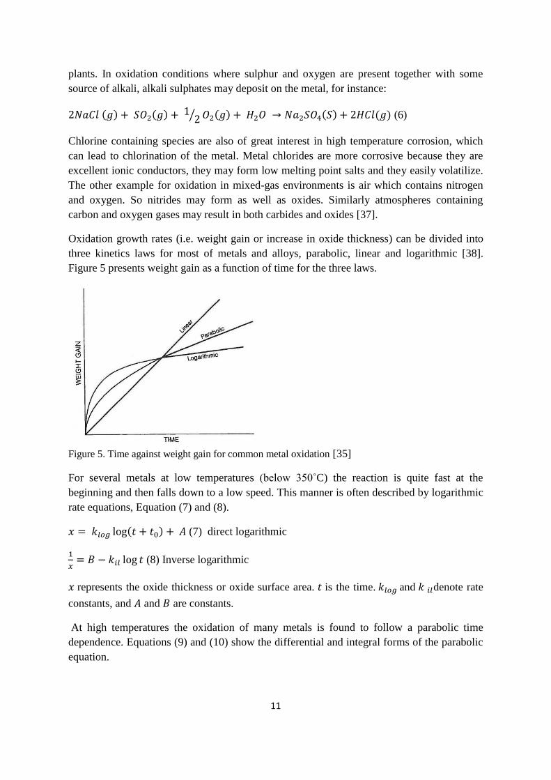
Oxidation growth rates (i.e. weight gain or increase in oxide thickness) can be divided into
three kinetics laws for most of metals and alloys, parabolic, linear and logarithmic [38].
Figure 5 presents weight gain as a function of time for the three laws.
Figure 5. Time against weight gain for common metal oxidation [35]
For several metals at low temperatures (below 350˚C) the reaction is quite fast at the
beginning and then falls down to a low speed. This manner is often described by logarithmic
rate equations, Equation (7) and (8).
(7) direct logarithmic
(8) Inverse logarithmic
represents the oxide thickness or oxide surface area. is the time. and denote rate
constants, and and are constants.
At high temperatures the oxidation of many metals is found to follow a parabolic time
dependence. Equations (9) and (10) show the differential and integral forms of the parabolic
equation.

12
(9)
(10)
Where and present the rate constants and is the integration constant.
Parabolic oxidation occurs when the oxide is an effective barrier and cations or oxygen ions
have to diffuse through the scale to react with each other. As the scale becomes thicker,
diffusion takes longer and the oxidation rate falls [35].
In parabolic and logarithmic equations reaction rates decrease with time. But in linear
oxidation, the rate is constant with time and is therefore independent of the amount of gas or
metal. Linear oxidation kinetics are given by
(11)
(12)
Where and are the rate constant and the integration constant respectively [39].
Linear oxidation occurs when the oxide layer does not form an effective barrier, for example
if it is cracked or porous [38].
5.5 Oxidation of different alloys
When an alloy containing different metals is surrounded by air, the oxide of metal, which
has the lowest Gibbs free energy, is the more stable. An alloy’s constituents differ with
respect to oxygen affinity and diffusivity in the alloy and in the oxide scale. These
differences are used in the design of oxidation-resistant alloys. Thus, high temperature alloys
contain constituents (e.g. chromium, aluminium, silicon) with a high oxygen affinity
intended to form an external protective scale (Cr2O3, Al2O3, SiO2). However these materials
may produce oxide in the form of precipitates in the interior of the alloy, so-called internal
oxidation [40].
5.5.1 Low alloy steels
Ordinary steels are essentially alloys of iron and carbon with small additions of elements
such as manganese and silicon added to provide the requisite mechanical properties. Low
alloy steel is widely used as a waterwall material. But low alloy steels corrode a lot both at
low and high temperature. In some conditions, adding 0.3% copper to the alloy can decrease
the corrosion rate by one quarter [41]. The elements phosphorus, chromium and nickel may
also improve resistance to corrosion. Formation of a dense, tightly adhering rust scale is a
factor in lowering the rate of attack. Oxidation of pure iron forms a multilayer scale and
below 570 ˚C the oxides Fe3O4 and Fe2O3 are stable. Over this temperature FeO can also be
formed [41].

13
5.5.2 Nickel alloys
Nickel alloys are employed for both high strength and outstanding corrosion resistance. This
is due to high chromium activity and diffusion rates at higher nickel contents [35]. Alloy 625
is a well-known commercial nickel-base alloy with high strength and high resistance against
pitting and high temperature corrosion. The strength of this alloy is a solid solution effect of
niobium and molybdenum which prevails during high temperature exposure.
5.5.3 Stainless Steels
Resistance to oxidation of stainless steels is related to the chromium content, Figure 6. Most
austenitic steels have at least 18% chromium and can be used at temperatures up to 870˚C.
Ferritic steels have usually lower oxidation resistance. When a high amount of chromium is
added to iron as an alloying element, a spinel oxide Fe(Fe,Cr)2O4 is formed. Spinel oxides
such as (Mg,Fe)(Al,Cr)2O4 may also form on stainless steels. Diffusion through this scale is
very slow and it is thus reduced the oxidation rate dramatically [28].
Figure 6. Effect of Chromium content on corrosion rate, test temperature 980 ˚C [42]

14
6. Experimental
All samples in this project were exposed in the Idbäcken heat and power plant. Idbäcken is
located in Nyköping, Södermanland, Sweden and supplies electricity and hot water for the
city. The plant consists of three boilers, two circulating fluidized bed boilers for hot water
and one bubbling fluidized bed boiler for combined heat and power (CHP). The latter was
the sample exposure place. The CHP boiler generates 35 MW of electricity and 69 MW of
heat. The final steam data is 540 °C and 140 bar. The pressure of 140 bar gives a maximum
water temperature of 340 °C and the tubes are assumed to have a metal temperature of 390
°C. Since 2008 the plant has used 100% waste wood as the fuel which increased the
corrosion rate rapidly. The boiler runs at quite low excess oxygen levels of 2-2.5%, but in
some parts of the boiler even lower than 1%. This helps to decrease NOx emissions and
increase efficiency.
6.1 Deposit samples
During the summer shutdown of 2011, deposits were scraped off from different positions on
the top of tube furnace walls. Figure 7 shows the position of all samples from different walls.
Most of the deposits were taken from areas in the boiler between the secondary and tertiary
air ports (height 11.5 to 18 m), where corrosion is worst. Two samples (F6 and F7) were
scratched from above the tertiary air ports (height 18 m). The samples vary in size, number
of particles, shape and colour.
6.2 Test panel tube samples
Test panels of the low alloy steel 16Mo3 were welded into the right wall of the boiler in
August 2008. Some of the tubes were arc-weld overlay coated with Alloy 625 and some
were left uncoated. Two tube specimens were cut out in August 2011. One sample is the
uncoated 16Mo3 sample as the reference tube (P4) and the other is the coated sample (P1).
The nominal chemical compositions of low alloy steel and coating material are shown in
Tables 3 and 4.
Table 3. Nominal chemical composition of 16Mo3 [43]
Element C Mn Si P S Cr Mo Ni Cu N Nb Fe
wt%
0.12-
0.2
0.4-
0.9
0.00-
0.35
0.000-
0.025
0.00-
0.01
0.00-
0.30
0.25-
0.35
0.00-
0.30
0.00-
0.30
0.00-
0.012
0.00-
0.020
Balance
Table 4. Nominal chemical composition of Alloy 625 [44]
Element Ni Cr Fe Mo Nb+Ta C Mn Si P S Al Ti Co[a]
wt% 58.0
min
20.0-
23.0
5.0
max
8.0-
10.0
3.15-
4.15
0.10
max
0.50
max
0.50
max
0.015
max
0.015
max
0.40
max
0.40
max
1.0
max
[a] If determined

15
Figure 7. Schematic drawing of a) left wall, samples position L1 to L5 b) right wall, samples position
R1 to R5 c) front wall, samples position F1 to F7 d) back wall, samples position B1 to B3
6.3 Fin wall probe samples
To compare the tube samples results with more controlled samples, air-cooled probes were
designed which can be inserted into the fin wall between two tubes. One probe (A2) was
installed in the back wall where the corrosion was thought to be highest. The other probe
(B2) was installed in the right wall, close to the test panels, where corrosion was known to
be less. They were exposed inside the boiler for 934 hours. Four specimens can be attached
on each probe, only some of the results are reported here (Table 5). The samples’ dimensions
are 48mm length, 6 mm thickness and 7 mm width. The temperature was measured by a
thermocouple placed centrally at the back of each specimen and could be controlled by
16
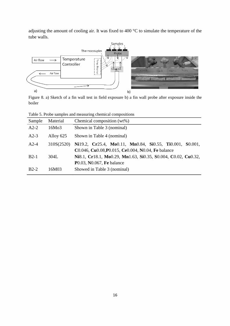
adjusting the amount of cooling air. It was fixed to 400 °C to simulate the temperature of the
tube walls.
Figure 8. a) Sketch of a fin wall test in field exposure b) a fin wall probe after exposure inside the
boiler
Table 5. Probe samples and measuring chemical compositions
Sample Material Chemical composition (wt%)
A2-2 16Mo3 Shown in Table 3 (nominal)
A2-3 Alloy 625 Shown in Table 4 (nominal)
A2-4 310S(2520) Ni19.2, Cr25.4, Mo0.11, Mn0.84, Si0.55, Ti0.001, S0.001,
C0.046, Cu0.08,P0.015, Ce0.004, N0.04, Fe balance
B2-1 304L Ni8.1, Cr18.1, Mo0.29, Mn1.63, Si0.35, S0.004, C0.02, Cu0.32,
P0.03, N0.067, Fe balance
B2-2 16M03 Showed in Table 3 (nominal)
a) b)

17
7 Analytical techniques
7.1 Scanning Electron Microscopy (SEM)
Scanning Electron Microscopy (SEM) was the main analysis method in this work, as it
provides a combination of high resolution imaging and large depth of focus. In SEM, a high-
energy-electron beam (1-30kV) is generated by the electron gun. The electron beam is
focused by some electromagnetic lenses and apertures to a fine probe (1-10 nm diameter).
The fine probe is aimed at a sample surface and scans it by scanning coils. When the fine
electron beam hits the sample, a variety of signals are generated, most importantly secondary
electrons, backscattered electrons, and X-rays, Figure 9 [45].
Figure 9. Schematic figure of the exited volume from the interaction between the electron beam and
specimen surface [45]
Secondary electrons (SE) are a result of inelastic interaction between the primary electrons
and the atoms in the specimen. SE can escape only from a thin region (less than 20 nm), so
they offer information on the surface topography.
Backscattered electrons (BE) are a result of the backward scattering of the primary electrons
and can escape from a larger region compared with SE. They offer information about
specimen composition.
When electrons interact with an atom, energy can be emitted as secondary electrons, an
electron from the outer shell can fill this vacancy. The corresponding energy to this
transition is released in the form of an X-ray photon, Figure 10. X-ray photons are
characteristic for each element and can be used to both quantify and qualify the elements
[46-47].

18
Figure 10. A backward direction of scattered electron as characteristic radiation [48]
SEM can combine with some techniques for chemical analyses, e.g. Energy dispersive
Spectroscopy (EDS) and Wavelength Dispersive Spectroscopy (WDS). In EDS the detected
X-ray signals can be shown in the form of a spectrum. The spectrum is the number of
photons by photon energy (keV). Each X-ray peak in the spectrum is related to a specific
element. EDS can be applied on a specimen to obtain a sample point (point analysis), in a
chosen area (area analysis) or the spatial distribution of the elements (traditional map or
QuantMaps map). WDS employs the X-rays diffraction on a crystal, so only photons with a
specific wavelength will drop onto the detector [49]. Table 6 shows differences between
EDS and WDS [48].
Table 6. Comparison of two chemical analysis techniques
EDS WDS
Energy Resolution 80-180 eV around 5 eV
Acquisition time 1 min 5-30 min
Use Easy difficult
Peak to background ratio 100:1 1000:1
In this work a JEOL 7001F and a JEOL 7000F were employed, with both EDS and WDS.
The devices were connected to an INCA system from Oxford Instruments. SEM parameters
were 15-20 keV and 16-18 A.
7.2 X-ray diffraction (XRD)
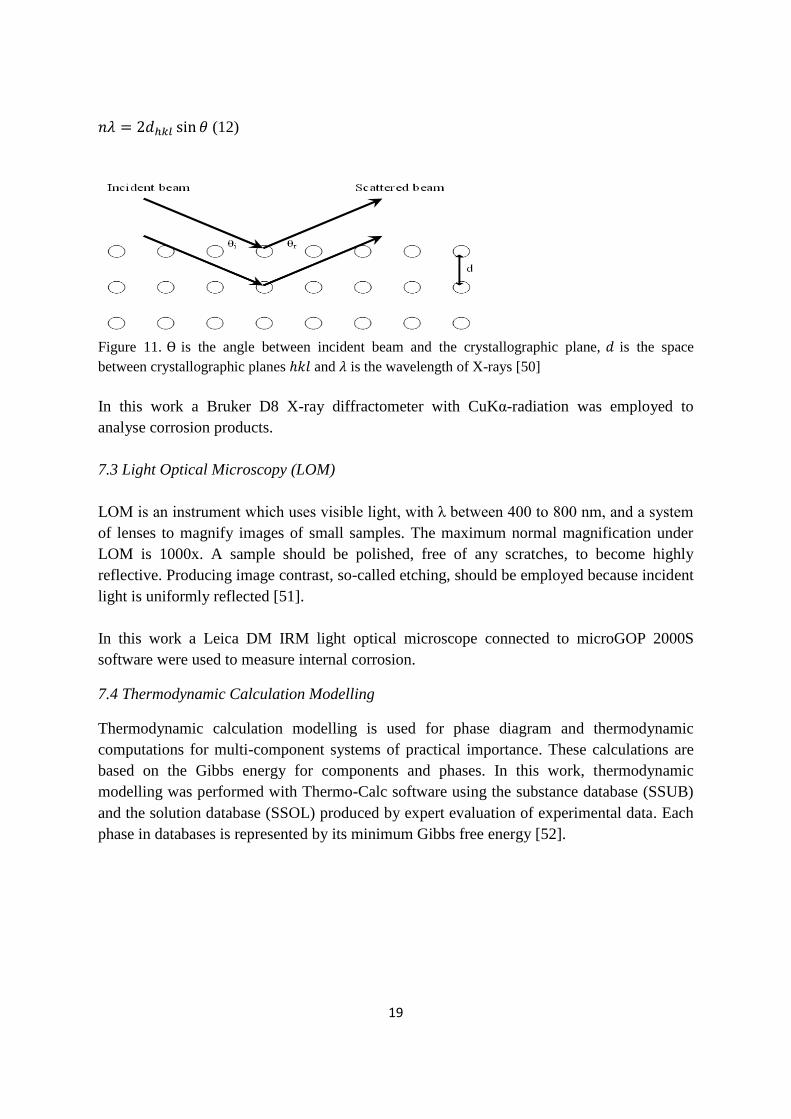
X-ray diffraction can be used to identify polycrystalline solids. In XRD a beam of
monochromatic X-rays is aimed at the specimen surface at an angle of Ɵ. When Bragg’s
law, Equation (12) and related Figure 11, is satisfied constructive interference occurs. By the
angles, different phases can be identified based on their dhkl [50].
19
(12)
Figure 11. is the angle between incident beam and the crystallographic plane, is the space
between crystallographic planes and is the wavelength of X-rays [50]
In this work a Bruker D8 X-ray diffractometer with CuKα-radiation was employed to
analyse corrosion products.
7.3 Light Optical Microscopy (LOM)
LOM is an instrument which uses visible light, with λ between 400 to 800 nm, and a system
of lenses to magnify images of small samples. The maximum normal magnification under
LOM is 1000x. A sample should be polished, free of any scratches, to become highly
reflective. Producing image contrast, so-called etching, should be employed because incident
light is uniformly reflected [51].
In this work a Leica DM IRM light optical microscope connected to microGOP 2000S
software were used to measure internal corrosion.
7.4 Thermodynamic Calculation Modelling
Thermodynamic calculation modelling is used for phase diagram and thermodynamic
computations for multi-component systems of practical importance. These calculations are
based on the Gibbs energy for components and phases. In this work, thermodynamic
modelling was performed with Thermo-Calc software using the substance database (SSUB)
and the solution database (SSOL) produced by expert evaluation of experimental data. Each
phase in databases is represented by its minimum Gibbs free energy [52].

20
8 Results
8.1 Deposit Samples
As a first step in identifying corrosion mechanisms, the parts of the deposit nearest to the
tubes were analysed under EDS and some by XRD.
8.1.1. SEM/EDS
Three separate areas, or three pieces of deposit in the case of smaller deposits, were analysed
under SEM. The scanned area was 5 mm2. There was not too much spread in chemical
composition within individual samples in these three areas under EDS, Figure 12.
Figure 12. Chemical compositions (at%) of three different particles in sample F4 (position four on
the front wall)
The deposits were attached to carbon tape for analysis, so the carbon contents were not
presented in analyses here. However, they were in the range 5 to 10 wt% for most of the
particles.
The average contents of elements which are thought to be corrosive or form corrosive salts
on all the furnace walls are presented in Table 7. An amount of nickel was detected in some
samples from the front wall, and comes from the coating Alloy 625. It was shown in the
table as well. The height value is from the bed of the boiler.
There was significant spread in chemical composition from position to position, but a higher
content of potassium was always associated with a high chlorine content, e.g. L1, R3, F4 and
B3. Potassium, chlorine and sulphur were found in all samples. However the amount varies a
lot. It is between 0.6 and 27.9 at% for chlorine. Sodium was present in all deposits except
R4. Lead was detected in 7 of 20 samples at low intensity, but high concentrations locally.

21
Lead was heterogeneously distributed and could be found as pure lead or in mixtures
containing oxygen as shown in Figure 13.
Table 7. Positions and average chemical compositions for the key elements (at%) of all Idbäcken
deposit samples scraped from the walls after the boiler shutdown in July 2011
Sample Wall Height
(m)
S Cl K Na Ni Zn Pb
L1 Left +12.5 3.5 21.2 15.5 10.9 -- -- --
L2 Left +12.5 4.4 4.4 7.1 5.5 -- 0.9 0.5
L3 Left +15 7.7 1.3 8.5 4.5 -- 2.7 0.8
L4 Left +15 3.8 2.0 5.0 3.7 -- 0.9 --
L5 Left +18 2.8 4.7 6.8 2.5 -- 0.89 --
R1 Right +14 5.6 0.8 4.6 1.0 -- 0.6 --
R2 Right +14 3.5 14.5 12.4 6.6 -- -- 0.6
R3 Right +18 2.4 27.9 15.4 18.1 -- -- 0.4
R4 Right +18 6.7 0.6 1.8 -- -- 1.1 1.1
R5 Right +18 5.6 0.9 6.3 2.9 -- 0.5 --
F1 Front +15 1.9 6.9 5.7 7.5 7.0 -- 1.6
F2 Front +15 2.2 3.3 5.7 7.5 0.4 0.2 --
F3 Front +18 1.3 12.8 10.6 1.8 -- 0.6 --
F4 Front +18 6.1 16.7 17.7 7.6 0.8 0.24 0.8
F5 Front +18 8.2 5.0 9.7 9.0 -- 1.7 --
F6 Front +21 1.9 10.9 8.3 5.0 -- -- --
F7 Front +21 5.4 10.1 13.1 6.1 -- 0.5 --
B1 Back +16 2.0 1.6 3.4 2.4 -- 0.7 --
B2 Back +16 4.2 13.2 11.8 8.2 -- 0.9 0.4
B3 Back +16 2.6 16.3 10.1 13.6 -- -- --
Figure 13. Island of Pb-Fe-Cl-O mixture in the sea of alkali chloride from sample F7, the analyses
are in at%.

22
Zinc was found in 15 of 20 samples at low concentrations. It was observed as crystals of
ZnCl2 , Figure 14.
Figure 14. Crystals of zinc chloride in sample of L3, the sample had the highest amount of Zn
The nickel which was detected in some samples, F1, F2 and F4, comes from the Alloy 625
coating.
8.1.2 XRD
Deposit particles of samples R4 (low chlorine content, 0.6 at%), F1 (medium chlorine
content, 6.9 at%) and R2 (high chlorine content, 14.5 at%) were separately ground and
analysed under X-ray diffraction. The X-ray diffraction results are shown in Table 8.
Table 8. Compounds recognized by XRD in samples R4, F1 and R2
Sample Identified compound in
strong intensity/high concentration
Identified compound in
medium intensity/medium concentration
R4 (K,Na)SO4, K2Pb(SO4)2 Pb2OSO4
F1 KCl NaCl, K3Na(SO4)2, NiO, K2Pb(CrO4)2
R2 KCl NaCl, K3Na(SO4)2, NiO, Cr1.6Fe1.4O4
In sample R4 (low chlorine content), sulphates dominated the XRD results. In sample F1
with a medium and R2 with a high chlorine content, potassium chloride dominated the XRD
results. Potassium-lead compounds were also identified. The presence of potassium lead
chromate in the deposit of sample F1, means that lead together with potassium had reacted
with the protective chromia layer and formed chromate, which is non-protective.
8.2 Test panel tube samples
8.2.1. Corrosion rate measurement
The thickness of the tube samples was measured after exposure at eight equally spaced
positions. The original wall thickness of the 16Mo3 tube sample (P4) was 7 mm and after
three years exposure (about 20000 hours) the average thickness of the examined section was
5.35 mm and the minimum 5.0 mm. The original thickness of the Alloy 625 welded coating

23
on the tube samples was about 4 mm, but being a welded structure it was difficult to measure
accurately and may have been greater than 4 mm in a number of areas. After 3 years
exposure the average thickness of the examined section was 3.8 mm and the minimum
thickness 3.4 mm.
These approximate values are normalized to 1000 hours and presented in Table 9.
Table 9. Metal loss from tube samples
Sample Average
(μm/1000h)
Maximum
(μm/1000h)
Position in
boiler
16Mo3 (P4) tube 82 (approx) 100 (approx) Right wall
Alloy 625 (P1) coated tube 10 (approx) 30 (approx) Right wall
8.2.2. SEM
The top of the two tube samples was polished by papers with grit P800, P1200, P2500 and
P4000 respectively. A polishing machine with the speed of 450 rpm was used in a dry
manner to avoid washing away the corrosion product on the tubes, especially chlorine which
is soluble in water. Polishing in this way facilitated the study of the base metal, oxide and
interface between oxide/substrate. The polishing method is shown in Figure 15.
Figure 15. Schematic drawings of tube samples before and after polishing
The elemental QuantMaps map for the Alloy 625 coated tube sample (see Figure 16) showed
concentrations of Pb and K in the oxide and at the substrate/deposit interface, but no Cl was
observed at interface. Low amounts of Cl (less than 1 wt%), were found in the oxide layer.
Figure 16. QuantMaps of key elements on the nickel-alloy coated tube sample
24
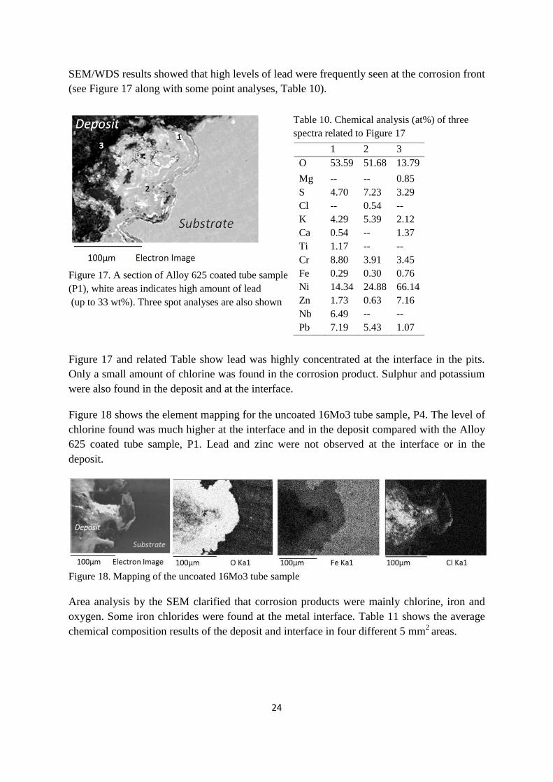
SEM/WDS results showed that high levels of lead were frequently seen at the corrosion front
(see Figure 17 along with some point analyses, Table 10).
Figure 17. A section of Alloy 625 coated tube sample
(P1), white areas indicates high amount of lead
(up to 33 wt%). Three spot analyses are also shown
Figure 17 and related Table show lead was highly concentrated at the interface in the pits.
Only a small amount of chlorine was found in the corrosion product. Sulphur and potassium
were also found in the deposit and at the interface.
Figure 18 shows the element mapping for the uncoated 16Mo3 tube sample, P4. The level of
chlorine found was much higher at the interface and in the deposit compared with the Alloy
625 coated tube sample, P1. Lead and zinc were not observed at the interface or in the
deposit.
Figure 18. Mapping of the uncoated 16Mo3 tube sample
Area analysis by the SEM clarified that corrosion products were mainly chlorine, iron and
oxygen. Some iron chlorides were found at the metal interface. Table 11 shows the average
chemical composition results of the deposit and interface in four different 5 mm2
areas.
1 2 3
O 53.59 51.68 13.79
Mg -- -- 0.85
S 4.70 7.23 3.29
Cl -- 0.54 --
K 4.29 5.39 2.12
Ca 0.54 -- 1.37
Ti 1.17 -- --
Cr 8.80 3.91 3.45
Fe 0.29 0.30 0.76
Ni 14.34 24.88 66.14
Zn 1.73 0.63 7.16
Nb 6.49 -- --
Pb 7.19 5.43 1.07
Table 10. Chemical analysis (at%) of three
spectra related to Figure 17
25
Table 11. Average chemical composition results for the oxide and interface of the uncoated tube
sample
wt% at%
O K 30.82 57.99
Cl K 15.22 12.92
Fe K 53.96 29.09
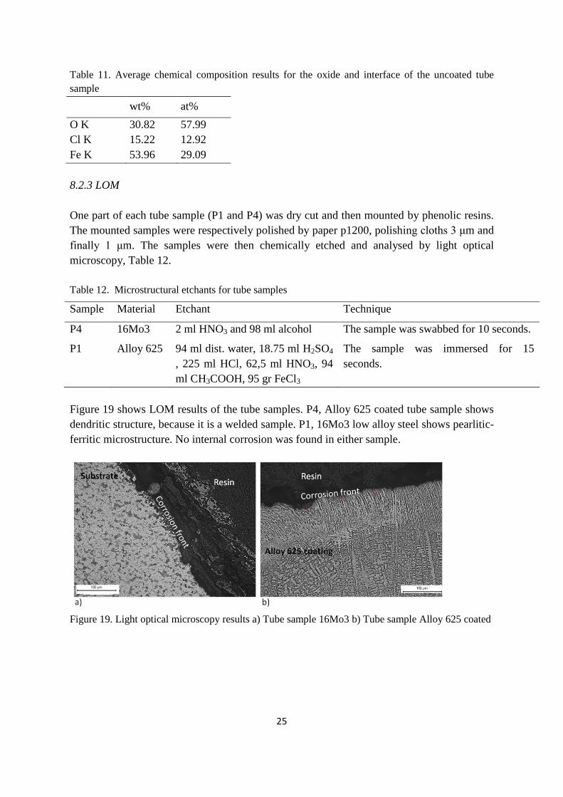
8.2.3 LOM
One part of each tube sample (P1 and P4) was dry cut and then mounted by phenolic resins.
The mounted samples were respectively polished by paper p1200, polishing cloths 3 μm and
finally 1 μm. The samples were then chemically etched and analysed by light optical
microscopy, Table 12.
Table 12. Microstructural etchants for tube samples
Sample Material Etchant Technique
P4 16Mo3 2 ml HNO3 and 98 ml alcohol The sample was swabbed for 10 seconds.
P1 Alloy 625 94 ml dist. water, 18.75 ml H2SO4
, 225 ml HCl, 62,5 ml HNO3, 94
ml CH3COOH, 95 gr FeCl3
The sample was immersed for 15
seconds.
Figure 19 shows LOM results of the tube samples. P4, Alloy 625 coated tube sample shows
dendritic structure, because it is a welded sample. P1, 16Mo3 low alloy steel shows pearlitic-
ferritic microstructure. No internal corrosion was found in either sample.
Figure 19. Light optical microscopy results a) Tube sample 16Mo3 b) Tube sample Alloy 625 coated
26
8.3 Fin wall probe samples
8.3.1 Corrosion rate measurement
The thickness of each specimen was measured before and after exposure at 4 places along
the centre-line. Before testing the thickness was measured with a micrometer. After testing
the specimens were sectioned (dry cutting) at the four places. Then the four parts of each
specimen were examined in an optical microscope with a micrometer measuring gauge. One
part was left unmounted. Table 13 shows the maximum thickness loss and the average
thickness loss which is normalised to 1000 hour.
Table 13. Metal loss from probe samples
Sample Average
(μm/1000h)
Max
(μm/1000h)
Position
in the boiler
16Mo3 (A2-2) 116 133 Back wall
Alloy 625 (A2-3) 47 55 Back wall
310S (A2-4) 61 75 Back wall
304L (B2-1) 54 78 Right wall
16Mo3 (B2-2) 78 97 Right wall
Sample A2-3 has the lowest corrosion rate among all samples as one might expect. The
metal loss of stainless steel samples are between the low alloy steel sample and the nickel
alloy sample.
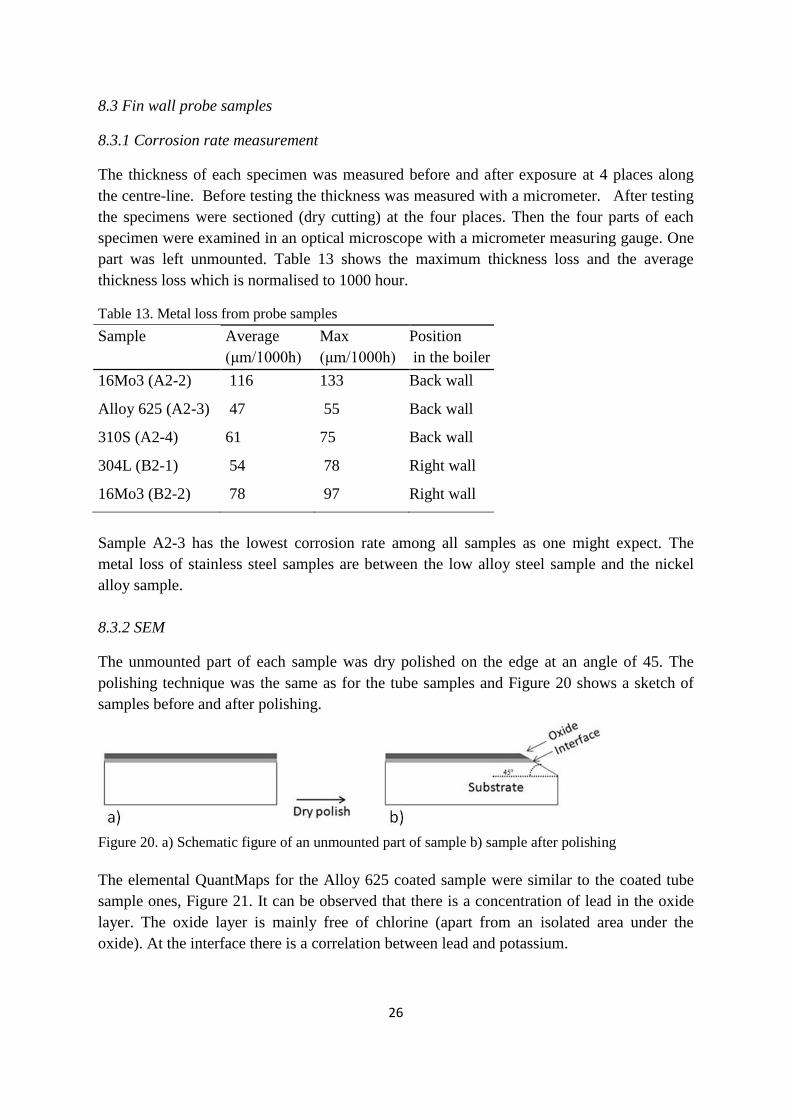
8.3.2 SEM
The unmounted part of each sample was dry polished on the edge at an angle of 45. The
polishing technique was the same as for the tube samples and Figure 20 shows a sketch of
samples before and after polishing.
Figure 20. a) Schematic figure of an unmounted part of sample b) sample after polishing
The elemental QuantMaps for the Alloy 625 coated sample were similar to the coated tube
sample ones, Figure 21. It can be observed that there is a concentration of lead in the oxide
layer. The oxide layer is mainly free of chlorine (apart from an isolated area under the
oxide). At the interface there is a correlation between lead and potassium.

27
Figure 21. QuantMaps of key elements on the nickel-alloy probe sample (A2-3)
Lead was present in the EDS point analysis, but not in combination with chlorine, Figure 22
and Table 14.
The 16Mo3 probe sample (A2-2, back wall) was analysed under SEM/EDS and QuantMaps
for this sample are presented in Figure 23. Chlorine was present at the interface and in the
deposit. No lead and sulphur was found at the corrosion front. Figure 24 and related table
(Table 15) elucidated that corrosion product is mainly iron, chlorine and oxygen.
Table 14. Chemical composition (at%) of two
spectra related to Figure 22
1 2
O 69.91 65.17
Na 4.41 10.81
Mg 1.35 1.17
Al -- 0.70
Si 0.82 1.00
S 9.17 9.45
Cl -- 0.62
K 6.12 7.08
Ca 3.27 1.22
Ti 0.38 --
Fe -- 0.42
Ni 0.77 2.36
Pb 3.78 --
Figure 22. A section of the surface of
nickel-alloy probe specimen with two
marked spectra

28
Figure 23. QuantMaps of the 16Mo3 probe sample
Figure 24. A section through the surface of 16Mo3
probe specimen on right wall with two marked spectra
These results are highly similar to those of the 16Mo3 probe sample on the right wall (B2-2).
Figure 25 shows SEM quantmapping of the sample. No lead and sulphur were present in the
corrosion product. Chlorine was observed in the deposit or at the interface between substrate
and oxide.
1 2
O 26.10 61.21
Si 0.48 0.70
S 0.30 0.24
Cl 1.02 7.66
K 0.09 --
Cr 0.25 --
Fe 71.76 29.94
Table 15. Chemical composition (atomic %) of
two spectra related to Figure 24
29
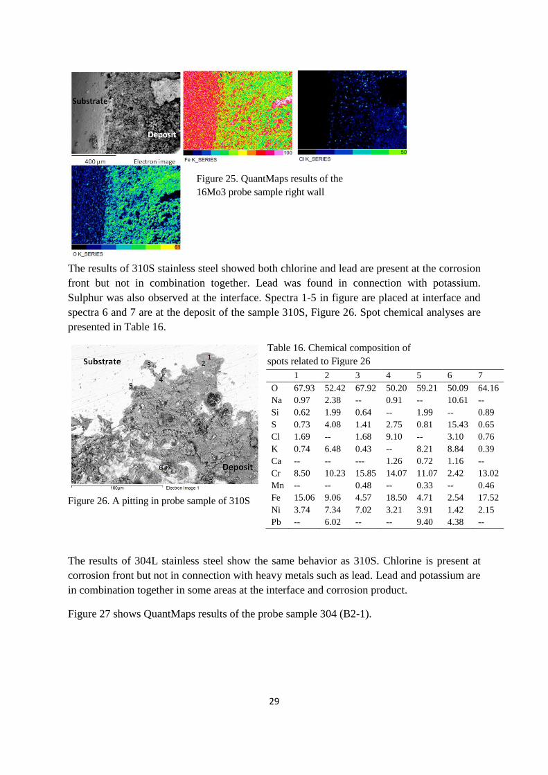
The results of 310S stainless steel showed both chlorine and lead are present at the corrosion
front but not in combination together. Lead was found in connection with potassium.
Sulphur was also observed at the interface. Spectra 1-5 in figure are placed at interface and
spectra 6 and 7 are at the deposit of the sample 310S, Figure 26. Spot chemical analyses are
presented in Table 16.
Figure 26. A pitting in probe sample of 310S
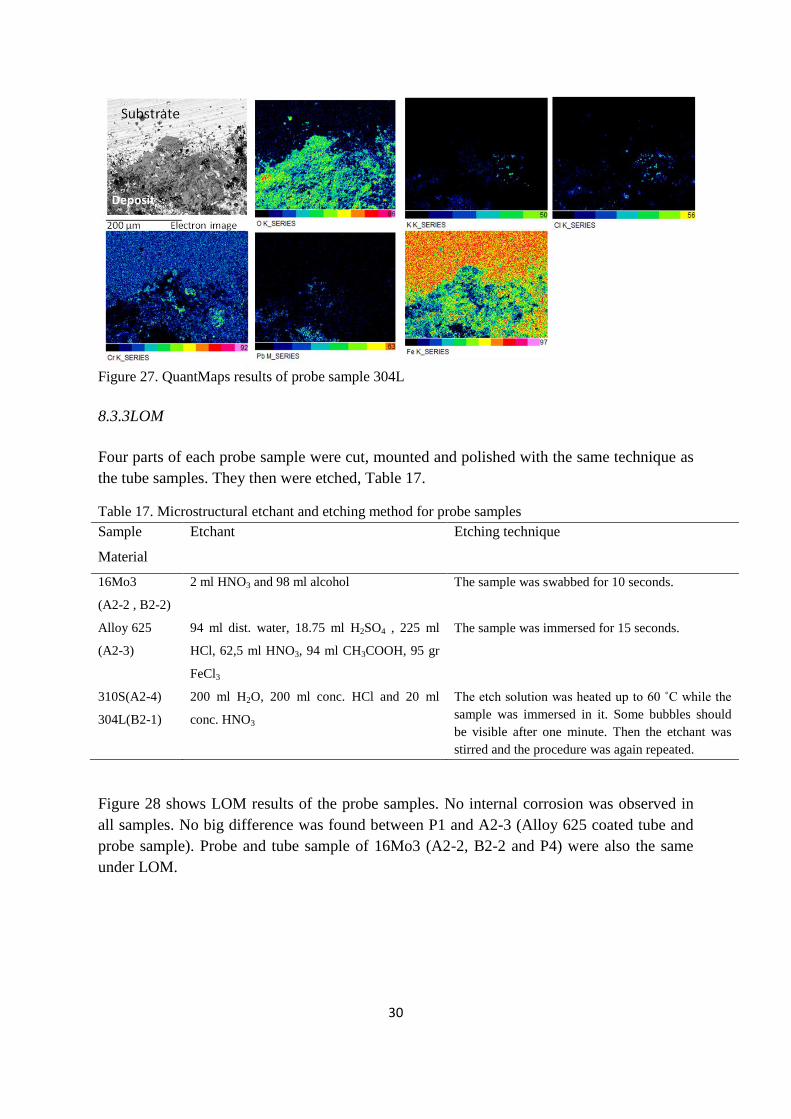
The results of 304L stainless steel show the same behavior as 310S. Chlorine is present at
corrosion front but not in connection with heavy metals such as lead. Lead and potassium are
in combination together in some areas at the interface and corrosion product.
Figure 27 shows QuantMaps results of the probe sample 304 (B2-1).
Figure 25. QuantMaps results of the
16Mo3 probe sample right wall
Table 16. Chemical composition of
spots related to Figure 26
1 2 3 4 5 6 7
O 67.93 52.42 67.92 50.20 59.21 50.09 64.16
Na 0.97 2.38 -- 0.91 -- 10.61 --
Si 0.62 1.99 0.64 -- 1.99 -- 0.89
S 0.73 4.08 1.41 2.75 0.81 15.43 0.65
Cl 1.69 -- 1.68 9.10 -- 3.10 0.76
K 0.74 6.48 0.43 -- 8.21 8.84 0.39
Ca -- -- --- 1.26 0.72 1.16 --
Cr 8.50 10.23 15.85 14.07 11.07 2.42 13.02
Mn -- -- 0.48 -- 0.33 -- 0.46
Fe 15.06 9.06 4.57 18.50 4.71 2.54 17.52
Ni 3.74 7.34 7.02 3.21 3.91 1.42 2.15
Pb -- 6.02 -- -- 9.40 4.38 --
30
Figure 27. QuantMaps results of probe sample 304L
8.3.3LOM
Four parts of each probe sample were cut, mounted and polished with the same technique as
the tube samples. They then were etched, Table 17.
Table 17. Microstructural etchant and etching method for probe samples
Sample
Material
Etchant Etching technique
16Mo3
(A2-2 , B2-2)
2 ml HNO3 and 98 ml alcohol The sample was swabbed for 10 seconds.
Alloy 625
(A2-3)
94 ml dist. water, 18.75 ml H2SO4 , 225 ml
HCl, 62,5 ml HNO3, 94 ml CH3COOH, 95 gr
FeCl3
The sample was immersed for 15 seconds.
310S(A2-4)
304L(B2-1)
200 ml H2O, 200 ml conc. HCl and 20 ml
conc. HNO3
The etch solution was heated up to 60 ˚C while the
sample was immersed in it. Some bubbles should
be visible after one minute. Then the etchant was
stirred and the procedure was again repeated.
Figure 28 shows LOM results of the probe samples. No internal corrosion was observed in
all samples. No big difference was found between P1 and A2-3 (Alloy 625 coated tube and
probe sample). Probe and tube sample of 16Mo3 (A2-2, B2-2 and P4) were also the same
under LOM.

31
Figure 28. Probe samples under optical microscopy a) 16Mo3 (back wall) b) 16Mo3 (right wall)
c) Alloy 625 coating d) 310S e) 304L
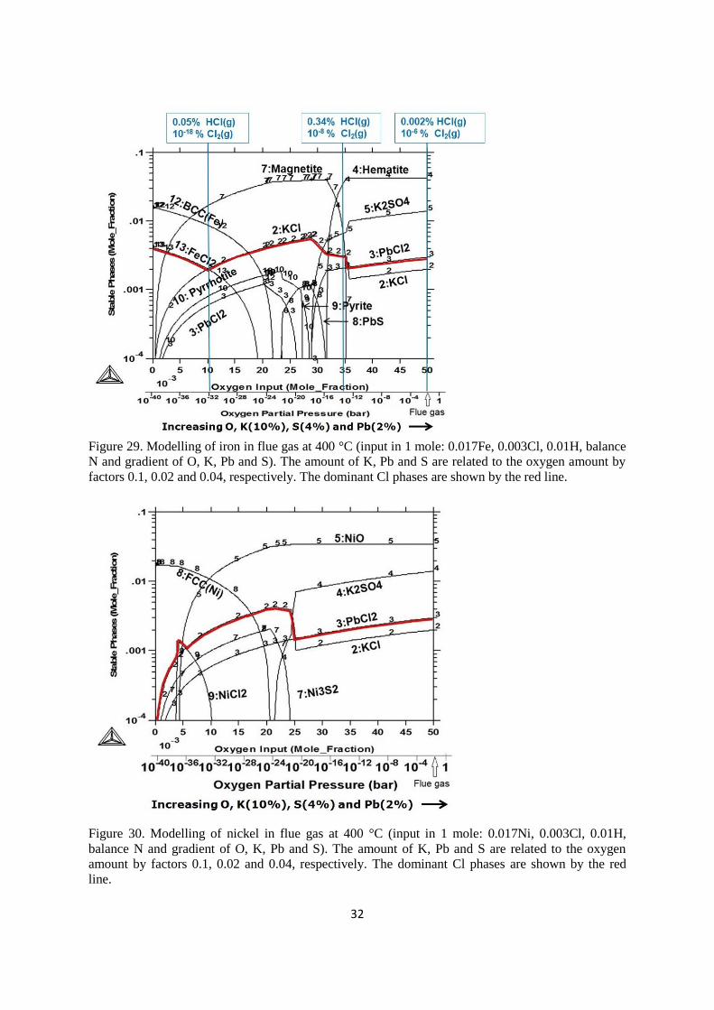
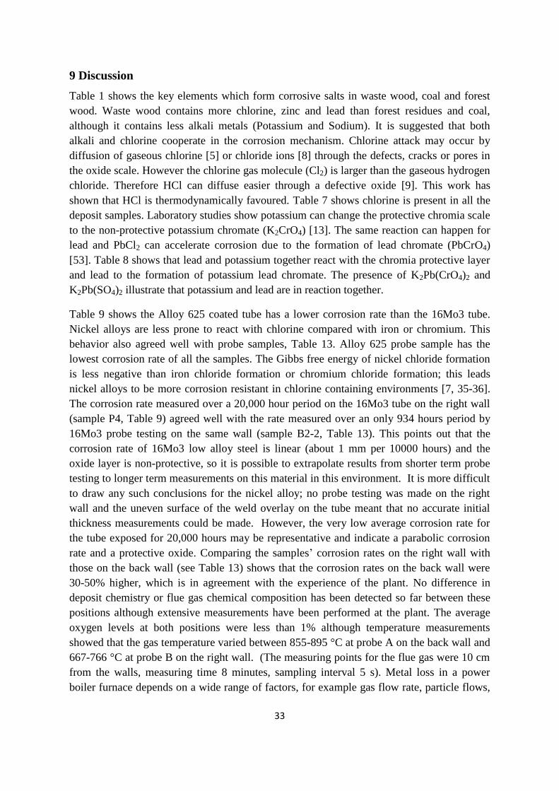
8.4 Thermo-Calcc results
Thermodynamically stable phases were modelled regarding corrosion and flue gas
composition at 400 ˚C by Thermo-Calc software. For simplification, chromium and
molybdenum were excluded from 16Mo3 alloy and Alloy 625 alloy. So, the simulation was
done using pure iron and pure nickel, Figure 29 and Figure 30.
The modelling was performed with a constant amount of iron or nickel, hydrogen and
chlorine, and increasing amounts of oxygen, sulphur, potassium and lead (It was not possible
to perform modelling with more than four elements as variables). The total amount of
species was set to one mole with nitrogen as balance. The gas species in equilibrium with the
solid phases is not shown in the diagrams. The gas phase mainly contains nitrogen, water
vapour and a small amount of hydrogen chloride. At high oxygen partial pressures the gas
phase also contains oxygen gas and at lower oxygen partial pressures it also contains
hydrogen gas, basically controlled by the hydrogen-oxygen-water equilibrium. The oxygen
gradient (partial pressure) is shown at the x-axis, the average of oxygen levels measured in
the flue gas is less than 1% in both cases which is marked with an arrow in the Figures 29
and 30. The expected stable phases in a corrosion product/deposited layer are shown in the
y-axis in both diagrams. The dominant Cl-containing phases are presented in both cases with
a red line. The dominating Cl-containing phases from low to high oxygen partial pressure
and sulphur partial pressure in Figure 29 are respectively FeCl2, KCl and PbCl2. In nickel
modelling (Figure 30) the phases are HCl, KCl(NiCl2), KCl, PbCl2. The amounts of chlorine
in hydrated form (HCl) and gaseous molecule chlorine (Cl2) are calculated in the iron case
and are shown at three different positions in blue boxes, Figure 29.
32
Figure 29. Modelling of iron in flue gas at 400 °C (input in 1 mole: 0.017Fe, 0.003Cl, 0.01H, balance
N and gradient of O, K, Pb and S). The amount of K, Pb and S are related to the oxygen amount by
factors 0.1, 0.02 and 0.04, respectively. The dominant Cl phases are shown by the red line.
Figure 30. Modelling of nickel in flue gas at 400 °C (input in 1 mole: 0.017Ni, 0.003Cl, 0.01H,
balance N and gradient of O, K, Pb and S). The amount of K, Pb and S are related to the oxygen
amount by factors 0.1, 0.02 and 0.04, respectively. The dominant Cl phases are shown by the red
line.
33
9 Discussion
Table 1 shows the key elements which form corrosive salts in waste wood, coal and forest
wood. Waste wood contains more chlorine, zinc and lead than forest residues and coal,
although it contains less alkali metals (Potassium and Sodium). It is suggested that both
alkali and chlorine cooperate in the corrosion mechanism. Chlorine attack may occur by
diffusion of gaseous chlorine [5] or chloride ions [8] through the defects, cracks or pores in
the oxide scale. However the chlorine gas molecule (Cl2) is larger than the gaseous hydrogen
chloride. Therefore HCl can diffuse easier through a defective oxide [9]. This work has
shown that HCl is thermodynamically favoured. Table 7 shows chlorine is present in all the
deposit samples. Laboratory studies show potassium can change the protective chromia scale
to the non-protective potassium chromate (K2CrO4) [13]. The same reaction can happen for
lead and PbCl2 can accelerate corrosion due to the formation of lead chromate (PbCrO4)
[53]. Table 8 shows that lead and potassium together react with the chromia protective layer
and lead to the formation of potassium lead chromate. The presence of K2Pb(CrO4)2 and
K2Pb(SO4)2 illustrate that potassium and lead are in reaction together.
Table 9 shows the Alloy 625 coated tube has a lower corrosion rate than the 16Mo3 tube.
Nickel alloys are less prone to react with chlorine compared with iron or chromium. This
behavior also agreed well with probe samples, Table 13. Alloy 625 probe sample has the
lowest corrosion rate of all the samples. The Gibbs free energy of nickel chloride formation
is less negative than iron chloride formation or chromium chloride formation; this leads
nickel alloys to be more corrosion resistant in chlorine containing environments [7, 35-36].
The corrosion rate measured over a 20,000 hour period on the 16Mo3 tube on the right wall
(sample P4, Table 9) agreed well with the rate measured over an only 934 hours period by
16Mo3 probe testing on the same wall (sample B2-2, Table 13). This points out that the
corrosion rate of 16Mo3 low alloy steel is linear (about 1 mm per 10000 hours) and the
oxide layer is non-protective, so it is possible to extrapolate results from shorter term probe
testing to longer term measurements on this material in this environment. It is more difficult
to draw any such conclusions for the nickel alloy; no probe testing was made on the right
wall and the uneven surface of the weld overlay on the tube meant that no accurate initial
thickness measurements could be made. However, the very low average corrosion rate for
the tube exposed for 20,000 hours may be representative and indicate a parabolic corrosion
rate and a protective oxide. Comparing the samples’ corrosion rates on the right wall with
those on the back wall (see Table 13) shows that the corrosion rates on the back wall were
30-50% higher, which is in agreement with the experience of the plant. No difference in
deposit chemistry or flue gas chemical composition has been detected so far between these
positions although extensive measurements have been performed at the plant. The average
oxygen levels at both positions were less than 1% although temperature measurements
showed that the gas temperature varied between 855-895 °C at probe A on the back wall and
667-766 °C at probe B on the right wall. (The measuring points for the flue gas were 10 cm
from the walls, measuring time 8 minutes, sampling interval 5 s). Metal loss in a power
boiler furnace depends on a wide range of factors, for example gas flow rate, particle flows,
34
flue gas chemistry, deposit chemistry and gas temperature or heat flux. In this case the
increase in flue gas temperature close to the back wall may account for the difference, in the
absence of any other factors.
Two forms of attack are thought to occur in waste environments: chlorine corrosion [5, 8-9,
27, 54] and alkali corrosion [29, 34], both initiating from the alkali- and chloride-rich
deposits and flue gas. The results of our investigations are in agreement with the
mechanisms.
The nickel-alloy coated tube specimen (Figure 16) shows the presence of potassium and lead
in the corrosion front. Only a small amount of chlorine was found in deposit. The nickel is
spreading from the oxide into the deposit which might suggest a fluxing mechanism. High
amounts of lead and potassium at the corrosion front on the nickel alloy coated tube are
measured by the spot analyses shown in Figure 17 and related table. XRD results (Table 8)
also show the formation of potassium lead chromate. The results of the Alloy 625 probe test
(Figure 21) were highly similar to the results of the Alloy 625 tube test. In Figure 22 and
related table (Table 14), the Alloy 625 probe sample also shows a concentration of lead in
the nickel oxide, an area which is devoid of chlorine. It appears then that the Alloy 625
coated samples are suffering from corrosion by a lead-potassium combination.
By contrast, chlorine was present at the interface between substrate and deposit of all the
16Mo3 specimens, but we did not detect any lead and potassium (see Figure 18, Figure 23
and Figure 25). Only small amounts of potassium were detected under SEM by point or area
analyses, Table 11 and Table 15. The dominant corrosion mechanism in 16Mo3 low alloy
steel seems to be chloride attack.
Stainless steels results (Figure 26 and Figure 27) show chlorine, lead and potassium at the
corrosion front. Lead and potassium are found together; however lead is not found with
chlorine at the corrosion front. It seems that 304L and 310S are attacked by mix of both
mechanisms: chloride containing species and lead-potassium combination. Table 13 shows
that the corrosion rates of 304L and 310S stainless steels are in between of 16Mo3 and Alloy
625.
Figure 19 and Figure 28 show there is no internal corrosion in the tube or probe specimens.
No special difference was observed in the structure of tube and probe Alloy 625 samples or
of 16Mo3 samples under optical microscopy.
As shown in the Thermo-Calc modelling (Figure 29 and Figure 30) the stable phases in
contact with the flue gas are metal oxides i.e. hematite and nickel oxide. In the presence of
chromium, spinel oxides containing chromium, iron (in the case of iron) and nickel (in the
case of nickel) are thermodynamically expected. In the presence of heavy metals like zinc
and lead, heavy metal chlorides may form as indicated in the modelling by lead chloride.
However, at sufficiently high oxygen partial pressures other lead containing phases may

35
form as shown by XRD data from the nickel-alloy coated tube, i.e. lead potassium chromate.
This phase is unfortunately not included in the Thermo-Calc data bases. Alkali chlorides
such as potassium chloride are also expected unless the sulphur and oxygen content is high
enough to convert potassium chloride to potassium sulphate [55]. This conversion tendency
towards potassium sulphate can be observed in the modelling at higher oxygen partial
pressures than 10-16
in the case of iron and 10-21
in the case of nickel, i.e. this process is
thermodynamically more favoured in the case of nickel.
At lower oxygen partial pressures (i.e. closer to the metal surface) the stability area of iron
chloride is much larger than that at nickel chloride. Obviously, nickel base alloys are
expected to be less prone to chlorine induced corrosion from a thermodynamic point of view.
The amount of HCl and Cl2 has been calculated by Thermo-Calc at different oxygen partial
pressures and three of the results are presented in Figure 29 in blue boxes. This shows that
chlorine gas exists at extremely low levels; instead the hydrated form is thermodynamically
favoured. The amount of HCl is much higher than Cl2 (or FeCl2). It can be expected that the
porosity (i.e. the gas phase in the deposit/oxide layer) is dominated by gaseous hydrogen
chloride in the whole oxygen partial pressure range. Therefore it suggested that chlorine
corrosion in the hydrated form can govern the chlorine induced corrosion under an oxide
layer where no alkali is found.

36
10 Summary of presented papers
10.1 paper i
The use of biomass as a fuel for power production is increasing and as the price of virgin
wood continues to rise, waste wood (recycled wood) is used more. However waste wood
contains more chlorine, zinc and lead, which are believed to cause an increase in the
corrosion rates.
Corrosion problems have occurred on the furnace walls of a fluidised bed boiler firing 100%
waste wood under low NOx conditions. As a first step to understanding the impact of the
fuel, deposits have been collected and analysed from a number of positions on the lower area
of furnace walls. A large part of the walls have been coated with the Ni-base alloy Alloy
625.
There was considerable spread in the deposit composition, but a higher potassium content
was always associated with a high chlorine content. Chlorine was found in all the deposit
samples, sometimes at very high levels (27 atomic%). Potassium and sulphur were found in
all the deposits samples and Na was found in most samples (19 of 20). Zinc was found in 15
of 20 samples at low concentrations. Lead was found in 7 of 20 samples at low average
concentrations, but high concentrations locally.
X-ray diffraction results showed the presence of K-Pb compounds, such as K2Pb(CrO4)2 in
the deposit and initial examination of the Ni-alloy coated tubes showed that lead was greatly
concentrated in pits at the corrosion front.
10.2 paper ii
In this work, furnace tubes coated with a nickel-based alloy were compared to the uncoated
tubes of the low alloy steel 16Mo3 after three years of exposure in the boiler. The nickel
alloy coating and uncoated material were also compared with more controlled testing on a
air-cooled probe lasting for about 6 weeks at 400 ˚C. The corrosion rates were measured and
the samples were chemically analysed by SEM/EDS/WDS and XRD methods. The corrosive
environment was also modelled with Thermo-Calc software to predict thermodynamically
the stability of the corrosion products.
The corrosion rates measured from the probe and tube samples of 16Mo3 agreed well with
each other, implying linear corrosion rates. The results also showed that the use of nickel
alloy coatings changes the corrosion mechanism, which leads to a dramatic reduction in the
corrosion rate. The simplified Thermo-calc results are in agree with identified phases in
corrosion product.

37
10.3 paper iii
The combustion of waste wood is becoming more widespread in Europe, because it is carbon
dioxide neutral and a renewable energy source, but with a lower cost than forest fuel.
However it is a heterogeneous fuel with a high amount of chlorine, alkali and heavy metals
which leads to more corrosion in boilers than with fossil fuel or forest fuel combustion.
In this work different alloys were exposed in the fin wall between two furnace wall tubes by
air-cooled probes in a waste wood-fired fluidised bed boiler. The analysed materials were
low alloy steel 16Mo3, nickel-alloy Alloy 625, stainless steel 310S and ferritic iron-
chromium-aluminium Kanthal APMT. The exposure time was 934 hours at 400 ˚C to
investigate corrosion rate, corrosion front, deposit compositions and corrosion mechanisms.
As expected 16Mo3 exhibited the highest corrosion rate. Alloy 625 and Kanthal APMT had
the lowest corrosion rates (about 40% of the rate for 16Mo3), closely followed by 310S
(50% of the 16Mo3 rate). The corrosion mechanisms were very different in different
materials: chloride attack in 16Mo3, a combination of K-Pb attack in Alloy 625, a mixture of
Cl and K-Pb attack in the stainless steel 310S, and Cl and K attack in Kanthal APMT.
Thermodynamic modelling showed chlorine gas exists at extremely low levels (less than 0.1
ppm); instead the hydrated form is thermodynamically favoured. Consequently chlorine can
attack low alloy steels by gaseous hydrogen chloride rather than chlorine gas as previously
proposed.

38
11 Conclusions
The deposit results showed a wide spread in chemical composition related to different
positions, although chlorine, potassium and sulphur were found in all the samples. The
results revealed the presence of K-Pb compounds.
The results showed that coating furnace tubes with Alloy 625 alloy reduces the corrosion
rate of the waterwalls significantly.
The dominant mechanism in the 16Mo3 specimens was chloride corrosion, while attack by a
potassium-lead combination appeared to be the dominant mechanism in the nickel-alloy
coated samples. The corrosion mechanism in 310S and 304L stainless steels were mixture of
both chlorine attack and potassium-lead attack.
The results revealed Alloy 625 has the lowest corrosion rate, the next lowest corrosion-rate
material is Kanthal APMT, then 310S and 304L, and finally 16Mo3 corrodes fastest. The
corrosion rate of the 16Mo3 low alloy steel seems to be linear. The Alloy 625 seems to have
a parabolic corrosion rate.
The simplified thermodynamic modelling fitted well with the identified phases in SEM
results. Thermo-Calc modelling revealed chlorine gas exists at extremely low levels (less
than 0.1 ppm); instead the hydrated form is thermodynamically favoured, i.e. gaseous
hydrogen chloride. So it suggested that chlorine corrosion in hydrated form can attack the
low alloy steel 16Mo3 rather than chlorine gas.

39
12 Future work
As the maintenance cost is high in power plants, it would be valuable to find alloys which
are more corrosion resistant than alloy 625 or less expensive.
Work is continuing to find fuel additives to reduce corrosion.
Depth profile of corrosion products will be analysed using Glow Discharge Optical Emission
Spectroscopy (GDOES) to learn more about inner and outer oxide compositions.
Thermo-Calc modelling seems to be a promising tool also for such complex systems as
corrosion in flue gas, but more work is needed to simulate alloy and flue gas chemical
composition closer to each specific case. Additionally, it would be desirable that
thermodynamic data of certain identified complex phases should be added to the
thermodynamic databases in the future.

40
13 Acknowledgements
This study would not have been possible without the guidance and the help of several
individuals and groups who extended their valuable assistance. This includes the coffee
machine at KTH.
First, I am sincerely grateful to Pamela Henderson for all her help, supervision, precious
advice and discussions at each stage of this work.
I would like to thank Peter Szakálos for his supervision on this project. He has been my
inspiration in this anti-corrosion work.
Konsortium för Materialteknik vid termiska Energiprocesser (KME) and Vattenfall are
gratefully thanked for the financial support.
I will never forget Peter Viklund’s valuable contributions to this work. I should thank a lot
Annika Stålenheim, Mattias Matsson and Tomas Leffler at Vattenfall Research and
Development, Chirster Forsberg and Seppo Simola at Vattenfall Nordik Heat, Rikard
Norling and Annika Talus at Swerea Kimab, Anders Hjörnhede at SP-Technical Research
Institute of Sweden for their excellent collaborations.
The entire colleagues in division of Surface and Corrosion Science at KTH Royal Institute of
Technology, who build a very nice and un-corrosive environment, are thanked. I like you
movie buddies, innebandy mates, poker pals, pub guys and fika talkative fellows.
Finally the golden thank you will go to my wife, Ghazal, for supporting me throughout all
my studies at university.
“All the conditions of happiness are realized in the life of the man of science.”
Bertrand Russell
41
14 References
[1] M.Z. Jacobson, J. Geophys., 2005, 110, D14105
[2] http://www.energimyndigheten.se/en/About-us/Press-/News/Checkpoint-2008-
Greenhouse-gas-emissions-can-be-sharply-reduced/ Swedish Energy Agency, 2008,
Accessed by 2013-01-08
[3] http://www.government.se/sb/d/2031/a/120088 Government Offices of Sweden, 2009,
Accessed by 2013-01-08
[4] B. Strömberg, S. S. Herstad, Bränslehandboken, 2012
http://www.varmeforsk.se/rapporter?action=show&id=2943 The fuel handbook, 2012,
Accessed by 2012-06-10
[5] E. Reese, H.J. Grabke, Werkst. Korros., 1992, 43, 547
[6] H.J. Grabke, E. Reese, M. Spiegel, Corros. Sci., 1995, 37, 1023
[7] A.Zahs, M. Spiegel, H.J. Grabke, Corros. Sci., 2000, 42, 1093
[8] N. Folkeson, T. Jonsson, M. Halvarsson, L-G. Johansson, J-E. Svensson, Mater. Corros.
2011, 62, 606
[9] P.Szakálos, P. Henderson, R. Petterson, Presented at Proceedings of the 16th
international
corrosion conference, Beijing, China, 2005
[10] T. Ishitsuka, K. Nose, Corros. Sci., 2002, 44, 247
[11] S. Enestam, Ph.D. Thesis, Åbo Akademi, Åbo, Finland, 2011
[12] Y.S. Li, Y. Niu, W.T. Wu, , Mater. Sci. Eng. A, 2003, 345, 64
[13] J. Pettersson, H. Asteman, J.-E. Svensson, L.-G. Johansson, Oxid. Met., 2005, 64, 23
[14] http://www.sciencedaily.com/articles/f/fossil_fuel.htm Science Daily, 2007, Accessed
by 2013-01-17
[15] http://www.eia.gov/cfapps/ipdbproject/IEDIndex3.cfm Independent Statistics and
Analysis, USA government, 2012, Accessed by 2013-01-16
[16] J.R. Katzer, Global Climate Change – the Technology Challenge: Coal and
Coal/Biomass-Based Power Generation, Springer, NC, USA, 2011, ISBN 978-90-481-3153-
2
42
[17] Statens Energiverk, An Introduction to Biofuel, Swedish bioenergy association, Sweden,
1985
[18]http://www.biomassenergycentre.org.uk/portal/page?_pageid=76,15049&_dad=portal&
_schema=PORTAL biomass energy center 2011, Accessed by 2013-01-17
[19] Y. Alipour, P. Viklund, P. Henderson, VGB PowerTech, 2012, 12, 96
[20] J. Jermer, A. Ekvall, C. Tullin, http://www.varmeforsk.se/reports?action=show&id=3288
Inventory of contaminations in waste wood , 2001, Accessed by 2013-03-11
[21] F.M. Steingress, Low Pressure Boilers , Homewood III American Technical Publishers,
USA, 2001, ISBN 0-8269-4417-5
[22] F.M. Steingress, H.J. Frost (2003). High Pressure Boilers , Homewood III American
Technical Publishers, 1994, ISBN 0-8269-4415-4
[23] Y. Chungen, L.A. Rosendahl, S.K. Kær, Prog. Energy. Combust. Sci., 2008, 34, 725
[24] H. Spliethoff, V. Siegle, http://www.magazine.ifrf.net/9903biomass1/stuttgart/stuttgart.pdf
Biomass Combustion in Germany New Services- Technical Supplement, 1999, Accessed by
2013-02-21
[25] K. Kerr, S.D. Probert, , Appl. Energy , 1986, 23, 233
[26] R. Deacon, J. DuPont, C. Kiely, A. Marder, P. Tortorelli, Oxid. Met., 2009, 72, 67
[27] L-G. Johansson, J-E. Svensson, E. Skog, J. Pettersson, C. Pettersson, N. Folkeson, H.
Asteman, T. Jonsson, M. Halvarsson, Presented at Proceedings of Sino-Swedish Structural
Materials Symposium, Beijing, China, 2007, pp. 35-39
[28] P. Viklund, Licentiate thesis, KTH Royal Institute of Technology, Stockholm, Sweden,
2011
[29] C. Pettersson, J. Pettersson, H. Asteman, J.-E. Svensson, L.-G. Johansson, Corros. Sci.,
2006, 48, 1368
[30] E. Reese, H.J. Grabke, Mater. Corros., 1993, 44, 41
[31] J. Pettersson, N. Folkeson, L.-G. Johansson, J.-E. Svensson, Oxid. Met. 2011, 76, 93
[32] H. P. Nielsen, F. J. Frandsen, K. Dam-Johansen, L. L. Baxter, Prog, Energy Combust.
Sci. 2000, 26, 283
[33] E.M. Levin, C.R. Robbing, H.F. McMurdie, Phase Diagrams for Ceramists, the
American ceramic society inc., Ohio, USA, 1969, ISBN 978-09-160-9404-1

43
[34] S.C.Cha, M.Spiegel, Corros, Eng. Sci. Tech., 2005, 40, 249
[35] P. Kofstad, High Temperature Corrosion, Elsevier Applies Science, New York, USA,
1988, ISBN 1-85166-154-9
[36] H.J.T. Ellingham, J. Soc. Chem. Ind. London, 1944, 63, 125
[37] A.S. Khanna: Introduction to High Temperature Oxidation and Corrosion, ASM
International, USA, 2002, ISBN 0-87170-762-4
[38] O. Kubaschewski, B.E. Hopkins, Oxidation of Metals and Alloys, Butterworths
Scientific Publications, London, UK, 1953, ISBN 1-11418-617-1
[39] P. Kofstad, High Temperature Oxidation of Metals, Wiley, New York, USA, 1966,
ISBN 19670181017
[40] N. Birks, G.H. Meier, F.S. Petit, Introduction to The High-Temperature Oxidation of
Metals, Cambridge University Press, UK, 2006, ISBN 978-0-521-48042-0
[41]Y.-N. Chang, F.-I. wei, J. Mater. Sci., 1989, 24, 14
[42] http://www.atlassteels.com.au/ Atlas specialty metals, Australia, 2002, Accessed by
2013-02-06
[43] http://www.springermaterials.com/docs/pdf/978-3-540-44760-3_145.html The Landolt-
Börnstein Database, 2009, Accessed by 2013-03-12
[44] http://www.specialmetals.com/documents/Inconel%20alloy%20625.pdf Special metals,
2006, Accessed by 2013-03-12
[45] A.J. Garratt-Reed, D.C. Bell, P. Nicholson, Energy Dispersive Analyses in The Electron
Microscope. Oxford: BIOS Scientific Publishers Limited, 2003, ISBN 1-85996-109-6
[46] I.M. Watt, Johnson Matthey Technology Centre, The Principle and Practice of Electron
Microscopy, Cambridge: Cambridge University Press, UK, 1997, ISBN 978-0-521-43591-8
[47] J. Goldstein, D.E. Newbury, D.C. Joy, C.E. Lyman, P. Echlin, E. Lifshin, L. Sawyer,
J.R. Michael, Scanning Electron Microscopy and X-Ray Microanalysis,Springer, Germany,
2003, ISBN 978-0-306-47292-3
[48]http://cime.epfl.ch/files/content/sites/cime2/files/shared/Files/Teaching/MSE_603_2011
_spri ng/Chapter%2013%20-%20EDX.pdf CiMe group, 2009, Accessed by 2013-03-13
44
[49] D. Brune, R. Hellborg, H.J. Whitlow, O. Hunderi, Scanning Electron Microscope with
Energy- and Wavelenght-Dispersive Spectrometry, Weinheim, Germany, 2007, ISBN 978-3-
527-28843-4
[50] Y. Waseda, E. Mastsubara, K. Shinoda, X-Ray Diffraction Crystallography Introduction
Examples and Solved Problems, 2011, Springer, Germany, ISBN 978-3-642-16634-1
[51] G. Petzow, Metallographic Etching, 1999, ASM international, USA, ISBN 0-87170-
633-4
[52] http://www.thermocalc.com/ Thermo-Calc Software®, 1997, Accessed by 2013-03-13
[53] D. Bankiewicz, S. Enestam, P. Yrjas, M. Hupa, Fuel Process. Technol., 2013, 105, 89
[54] K.O. Davidsson, L.-E. Åmand, B. Leckner, B. Kovacevik, M. Svane, M. Hagström,
J.B.C. Pettersson, J. Pettersson, H. Asteman, J.-E. Svensson, L.-G. Johansson, Energy- Fuel.,
2007, 21, 71
[55] P. Henderson, P. Szakálos, R. Pettersson, C. Andersson, J. Högberg, Mater. Corros.,
2006, 57, 128