High-Resolution Methodology for Particle Size Analysis of Naturally Occurring

Sand Size Sediment Through Laser Diffractometry WITH Application to Sediment

Cores: Kismet, Fire Island, New York

A Thesis Presented

by

Kara Alexandra Dias

to

The Graduate School

in Partial Fulfillment of the

Requirements

for the Degree of

Master of Science

in

Geosciences

(Sedimentology)

Stony Brook University

May 2014

Copyright by Kara Alexandra Dias

2014

 

ii    

Stony Brook University

The Graduate School

Kara Alexandra Dias

We, the thesis committee for the above candidate for the

Master of Science degree, hereby recommend

acceptance of this thesis.

Michael Sperazza – Thesis Advisor Assistant Professor, Department of Geosciences

Troy Rasbury – Chairperson of Defense Associate Professor, Department of Geosciences

Gilbert N. Hanson – Second Reader Distinguished Service Professor, Department of Geosciences

This thesis is accepted by the Graduate School

Charles Taber Dean of the Graduate School

 

iii    

Abstract of the Thesis

High-Resolution Methodology for Particle Size Analysis of Naturally Occurring

Sand Size Sediment Through Laser Diffractometry WITH Application to Sediment

Cores: Kismet, Fire Island, New York

by

Kara Alexandra Dias

Master of Science

in

Geosciences

(Sedimentology)

Stony Brook University

2014

The detailed methodological measurements of very fine-grained sediments by laser diffraction have been reported to yield a very low analytical uncertainty. When coarser grained samples are run under the methodology recommended for fine-grained sediments, there is variability between the measurements, especially in the size fraction <200um. This study seeks to refine the standard operating procedures of laser diffraction for grain size analysis of sand sized sediment as well as quantify the associated analytical uncertainty. The influence of selected methodological aspects on the results of the particle size distribution were assessed and optimal machine parameters, suspension mediums and sample preparation techniques were determined. It was found that for the investigated sands the following modifications to the standard operating procedures for fine grained sediment must be made: (1) bulk dry sieving of the samples must be introduced as a sample preparation step, (2) optimal obscuration occurred between 15-25%, (3) optimal pump speed was 2600 rpm. The associated analytical uncertainty is ~1.7% at 2 sigma. This enriched methodology allows for an efficient and accurate means of grain size analysis of naturally occurring sand sized sediment.

The refined standard operating procedure is then applied to five sediment cores taken in a shoreline normal transect across Kismet, Fire Island, New York as well as

 

iv    

modern sediments from the well-developed barrier island facies. The enhanced resolution associated with the refined methodology allows for grain size to begin to be used as a proxy of barrier island depositional environment and for sediment cores to be analyzed at centimeter scale intervals. The study confirms previous research that statistically analyzing grain size data can be used as a method for facies modeling. This study introduces a new method of recognizing clusters in the data through the use of an unsupervised k-means clustering algorithm. The algorithm can efficaciously be applied to the data as an unbiased, efficient way to recognize clusters in the statistically analyzed grain size data as well as in the grain size data plotted with depth. Successfully developing a high resolution method for grain size analysis of sand sized particles and using this method to analyze sediment core samples to test and confirm the methods of barrier island facies modeling of others, this study sets up the ability to take on further sedimentologic studies to address the evolution of barrier island systems through 3D subsurface modeling.

 

v      

Table of Contents

List of Figures……………………………………………………………………………vii

List of Tables…………………………………………………………………………..…ix

Acknowledgements………………………………………………………………...……...x

Chapter 1: Introduction…………………………………………...……………………….1

Chapter 2: Methodology: High-Resolution Analysis of Naturally Occurring Sand Size

Sediment Through Laser Diffractometry…………………………………...……………..5

2.1 Background……………………………………………………………………5

2.2 Experimental Section………………………………………………………….6

2.2.1 Instrumentation……………………………………………………...6

2.2.2 Sample Preparation………………………………………………….8

2.2.3 Optimizing Machine Parameters……………….…………………..12

2.3 Results and Discussion………………………………………………………15

2.3.1 Subsampling and Aliquot Introduction…………………………….15

2.3.2 Dispersant and Medium…………………………………………....17

2.3.3 Obscuration………………………………………………………...19

2.3.4 Pump Speed……………………………………...……………….. 21

2.3.5 Measurement Duration……..………………………...………….... 23

2.4 Methodology Conclusions………………………………………………….. 24

Chapter 3: Grain Size as a Proxy of Depositional Environment Through Assessment of

Sediment Cores from Kismet, Fire Island, New York…………………………………...32

3.1 Study Area…………………………………………………………………...32

3.2 Methods………………………………….....………………………………..33

 

vi    

3.2.1 Core Collection…………………………………………………….34

3.2.2 Visual Description…………………………………………………36

3.2.3 Grain-Size Analysis………………………………………………..38

3.2.4 Statistical Analysis…………………………………………...…….39

3.3 Results and Discussion………………………………………………...…….43

3.4 Conclusions……………….………………………………...………………..62

Chapter 4: Implications……………………………………………………………..……68

References………………………………………………………………………………..70

Appendix……………………………………………………………………………...….79

 

vii    

List of Figures

Figure 1: Photograph of Stony Brook University’s Laser Diffractometer…………...…...6

Figure 2: Schematic Showing Major Elements of Malvern Mastersizer 2000…………....7

Figure 3: Detailed Schematic Diagram of the Inside of Malvern Mastersizer 2000…..….7

Figure 4: Histograms of the Five Samples Used Throughout this Study………………....9

Figure 5: Aliquot Introduction Methods- Dried vs. Pipette……………………………...16

Figure 6: Suspension Mediums…………………………………………………………..18

Figure 7: Obscuration Effects on Median Grain Size……………………………………20

Figure 8: Pump Speed Effects on Median Grain Size………………………………..….22

Figure 9: Time Effects on Median Grain Size……………………………………...……24

Figure 10: Particle Size Distributions-Standard Operating Procedures vs. Refined

Methodology……………………………………………………………………..29

Figure 11: Field Work Location-Kismet, Fire Island, New York…………………..…....33

Figure 12: Core Drilling…………………………………………………………..……...35

Figure 13: Core Extraction………………………………………………….……………35

Figure 14: Photograph of Sediment Cores A, B1, C1 and C2………………..………….37

Figure 15: Core A-Cross Bedding and Peat Nodules………………………………..…..44

Figure 16: Kismet Cores-Depth vs. Median Grain Size……………………………..…..46

Figure 17: Particle Size Distributions of the Modern Environments…………………….48

Figure 18: Median Grain Size vs. Skewness………………………………………...…..49

Figure 19: Direct Comparison of Median Grain Size vs. Skewness Between this Study

and a Similar Study on Mustang Island, TX……………………………...…...…50

 

viii    

Figure 20: Median Grain Size vs. Kurtosis………...…………………………………….52

Figure 21: Skewness vs. Kurtosis: Data Distribution about the Normal ……...……...…52

Figure 22: K-means Clustering applied to Median Grain Size vs. Skewness………...…53

Figure 23: K-means Clustering applied to Median Grain Size vs. Kurtosis………......…53

Figure 24: K-means Clustering applied to Core A Depth vs. Median Grain Size……….54

Figure 25: K-means Clustering applied to Core B1 Depth vs. Median Grain Size……...54

Figure 26: K-means Clustering applied to Core C1 Depth vs. Median Grain Size…..….55

Figure 27: K-means Clustering applied to Core C2 Depth vs. Median Grain Size…..….55

Figure 28: Stratigraphic Columns Placed in Geographic Context in a Cross Section of

Kismet, Fire Island……………………………….……………………...……….57

 

ix    

List of Tables

Table 1: Sediment samples used. ………………………………………………….…….9

Table 2: Suspension mediums used and the corresponding refractive indices. ..……….11

Table 3: Summary of experimental results from this study. ………………………….25

Table 4: Mean, standard deviation and skewness with associated environments. ……..56

 

x  

Acknowledgments

I would like to express my gratitude to my thesis committee including Dr. Michael Sperazza, Dr. Troy Rasbury and Dr. Gilbert Hanson. Particularly, I would like to acknowledge my advisor, Michael, for his guidance with the laser diffractometry and his encouragement and support to follow and develop my personal research interests through the second portion of this study. Without him, none of this would have been possible.

I extend special thanks to Dr. Bret Bennington and Dr. Christa Farmer at Hofstra University for allowing me to use their Vibracoring system and accompanying me in the field. I would like to thank Michael Bilecki, chief, National Park Service for his guidance in obtaining a permit to conduct the research on Fire Island National Seashore.

Lastly, I extend my gratitude to my family and friends for their unwavering support and encouragement during my time in graduate school. Especially, Courtney Melrose and Gina Shcherbenko for their enthusiastic attitude towards collecting sediment cores on a windy December weekend. To my parents, Dr. Anthony Jay and Patricia Dias, thank you for everything.

 

1    

Chapter 1

Introduction

Determination of grain size is one of the most essential measures in a

sedimentologic study. Grain size distributions are an important source of information

when interpreting the sedimentary environment. Advances in laser diffractometry have

significantly improved the precision and efficiency of grain size analysis. As a result,

this technique is becoming increasingly more popular over the past 20 years as a

sedimentologic tool (LOIZEAU et al. 1994; BEUSELINCK et al. 1998; SPERAZZA et al. 2004;

ESHEL, et. al., 2004; BLOTT AND PYE, 2006; RYZAK AND BIEGANOWSKI, 2011). Laser

diffraction has even replaced sieving to determine particle size distribution of lunar

samples by NASA due to the method’s high levels of reproducibility, speed of analysis

and small amount of sample required (COOPER, et. al., 2012). Still, the use of laser

diffraction technology has not entirely replaced the classical grain size determination

methods (ex: sieving, pipette and settling tube) and when selecting a method the pros and

cons of each must be considered. Compared with these classic methods, a disadvantage

of laser diffraction is the high cost of instrumentation (ESHEL, et. al., 2004). An

additional factor hindering the adaptation of the laser diffraction method is the

insufficient confidence in the results (FERRO et al. 2009; BUURMAN et al. 1997).

Sperazza (2004) has shown that laser diffraction can measure very fine-grained sediments

with high precision and low uncertainty. Careful application of laser diffraction

techniques can yield total uncertainty (method plus machine error at the 95% confidence

interval) of 6% or less for very-fined grained sediments (SPERAZZA et al. 2004). The first

goal of this study, presented in Chapter 2, is to establish a set of standardized sample

 

2    

preparation procedures and laser diffraction machine parameters for naturally occurring

sand size sediment that will result in low total uncertainty similar to that of very-fine

grained sediments. This methodology development will expand the scope of laser

diffraction techniques for particle size analysis and make possible a new range of

sedimentologic studies such as barrier island migration and dynamics of sediment

transport associated with beach erosion.

The record of grain size variability can be developed into a time-series data set,

called a proxy. A proxy data set is utilized as a substitute for one or more climatic,

environmental, or physical conditions that existed in the past but cannot be measured

directly. Traditional use of grain-size data in paleoclimate studies state that grain size can

serve as a proxy for aridity, wind strength and monsoon intensity (XIAO, et. al., 1995;

VANDENBERGHE, 1997; LU, et. al., 1998; STUUT, et. al., 2002; PENG, 2005). The

increased resolution in the grain size data has made it possible to create a stacked climate

record of the Quaternary period using grain size measurements of a loess sequence and

correlate this relative proxy data with the δ18O record from deep-sea sediments (DING, et.

al., 2002). The loess-paleosol record can be correlated almost cycle by cycle with the

marine record (DING, et. al., 2002). Additionally, a grain-size proxy was derived to aid in

the prediction of radionuclide activity of salt marshes and mud flats (CLIFTON, et. al.,

1999).

The environmental interpretation of grain-size distributions found in sedimentary

deposits has been, and currently is, a fundamental goal of sedimentology (MASON AND

FOLK, 1958; MCLAREN AND BOWLES, 1985; PEDREROS, et. al., 1996; SUTHERLAND AND

LEE, 1994; ERGIN, et. al., 2007; GUEDES, et. al., 2011). Grain size analysis has been used

 

3    

to distinguish environments based on parameters of the lognormal distribution. Median

grain size, sorting (standard deviation) and skewness of grain size data are the most

common sediment parameters analyzed when attempting to identify the direction of

sediment transport and the associated sedimentary processes of deposition (MCLAREN

AND BOWLES, 1985; PEDREROS, et. al., 1996; SIMMS, 2006; HAJEK, et. al., 2010). These

correspond to the first, second and third moment of the data distribution (HAZEWINKEL,

1993; PROKHOROV, 1990). The mean is the first moment. The variance, which is the

positive square root of the standard deviation, is the second moment and is related to the

sorting of a grain size distribution (HAZEWINKEL, 1993; PROKHOROV, 1990). The third

moment of the dataset is skewness and is the first dimensionless moment (HAZEWINKEL,

1993; PROKHOROV, 1990). Skewness is a statistical analysis often applied to datasets to

assess the degree of asymmetry and reflects changes in the tails of the distribution

(MASON AND FOLK, 1958; MCLAREN AND BOWLES, 1985; PEDREROS, et. al., 1996). The

analysis of grain size is especially an important source of information in situations where

sedimentary structures and/ or outcrops are not available or only slightly apparent

(GUEDES, et. al., 2011). These characteristics occur frequently in coastal Quaternary

deposits, such as barrier islands, where grain size analysis has been applied as a tool for

sedimentary facies discrimination (GUEDES, et. al., 2011; ERGIN, et. al., 2007; SIMMS,

2006; ABUODHA, 2003; MASON AND FOLK, 1958). For example, median grain size from

sediment cores was utilized by Simms (2006) as a relative proxy for changes in the

sedimentary facies between dune, barrier flat, inlet, shoreface and marine, to study the

Holocene evolution of the Mustang Island barrier island system, Texas. These grain size

data contributed to the researchers’ understanding of the environments and their changes

 

4    

over time. The second goal of this study, presented Chapter 3, is to test the use of grain

size analysis as a tool for sedimentary facies discrimination for the Fire Island barrier

island system. Development of this method for facies recognition will allow for deeper

questions, out of the scope of this study, to be addressed involving the recent evolution

and migration of the barrier island system through deeper sediment core analysis from

various transects on Fire Island and subsurface modeling through correlations and ground

penetrating radar.

 

5    

Chapter 2

Methodology: High-Resolution Analysis of Naturally Occurring Sand Size Sediment

Through Laser Diffractometry

Background

Grain size analysis using laser diffractometry or low-angle laser light scattering is

based on the principle that particles of a given size diffract light at a given angle. This

angle of diffraction is inversely proportional to the particle size. Laser diffraction

systems pass a laser beam of known wavelength through a suspension (liquid or aerosol)

and measures the angle and intensity of the diffracted light by the particles in the

suspension. The diffracted light is measured by detectors and then compared against a

theoretical model based on diffraction of particles with particular properties and size

distribution. The two main diffraction theories used in the determination of laser particle

size results but will not be discussed here are the Fraunhofer theory and Mie theory (see,

(LOIZEAU et al., 1994; MCCAVE et al., 1986; SINGER et al., 1988; WEBB, 2000; WEN et

al., 2002). The difference between the measured and theoretical diffraction patterns is the

residual value. This is the portion of the measurement results that is unexplained by the

theoretical model; therefore, minimizing this residual value reduces the machine

uncertainty (SPERAZZA et al. 2004).

 

6    

Experimental Section

Instrumentation

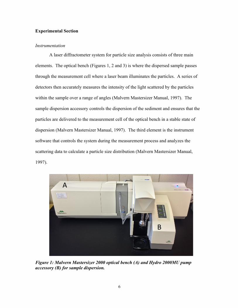
A laser diffractometer system for particle size analysis consists of three main

elements. The optical bench (Figures 1, 2 and 3) is where the dispersed sample passes

through the measurement cell where a laser beam illuminates the particles. A series of

detectors then accurately measures the intensity of the light scattered by the particles

within the sample over a range of angles (Malvern Mastersizer Manual, 1997). The

sample dispersion accessory controls the dispersion of the sediment and ensures that the

particles are delivered to the measurement cell of the optical bench in a stable state of

dispersion (Malvern Mastersizer Manual, 1997). The third element is the instrument

software that controls the system during the measurement process and analyzes the

scattering data to calculate a particle size distribution (Malvern Mastersizer Manual,

1997).

Figure 1: Malvern Mastersizer 2000 optical bench (A) and Hydro 2000MU pump accessory (B) for sample dispersion.

A  

B  

 

7    

Figure 2: Schematic showing the major elements of the Malvern Mastersizer 2000 laser diffractometer optical bench. Image from (JACKSON, 2011).

Figure 3: Schematic diagram of the Malvern Mastersizer 2000 laser diffractometer providing more detail on the internal diffraction components. The laser light is focused by Reverse Fourier Optics (RL) and collected by backscatter (BS), forward angle (FA) and large angle (LA) detectors. Other labeled components are the focal plane detector (FP), obscuration detector (TR), laser power monitor (MR) and measurement cell (MC). Figure from (SPERAZZA, et. al., 2004).

The instrumentation set up for this methodology study utilized a Malvern

Mastersizer 2000 laser diffractometer with a Hydro 2000MU pump (Figure 1). The

pump accessory continuously pumps the suspension through the laser diffractometer cell.

This continuous pumping ensures random orientation of the particles to the laser beam as

well as randomly sampling the suspended material (BEUSELINCK et al. 1998). The laser

 

8    

diffractometer utilizes two light sources; a blue LED laser at 0.466 micrometers (µm) and

a red He- Ne laser at 0.632 micrometers (µm) (Figures 2 and 3). The diffracted light

from the low-angle laser light scattering is measured by 52 sensors and collected into 100

size fraction bins (Figures 2 and 3). The Mastersizer 2000 takes 1000 measurements per

second. The grain size analyses reported are the average of three successive laser

diffraction runs of 12 seconds each. Measurement data was compiled with Malvern’s

Mastersizer 2000 software version five. Before accepting a grain size analysis, results

were first order inspected with the software to check for any anomalous results that could

be attributed to air bubbles, machine spikes or other operational errors. The software

utilizes Mie theory to convert the scatter of light energy to grain size and reports grain-

size distributions as volume percentage for each size bin (SPERAZZA et al. 2004).

Sample Preparation

Subsampling and Aliquot Introduction- Sample refers to the bulk sediment

collected from the outcrop, sediment core, soil, etc. In the case of this study, sample

refers to the loose beach sand collected from various locations on Long Island and one

from Australia to represent the naturally occurring material (Table 1). The bulk samples

were dry sieved (TxDOT, 1999) with the number 14 sieve, 1.4 millimeters, this was a

safety measure so not to exceed the maximum size fraction that can be pumped through

the Hydro 2000MU pump accessory. The subsample is the portion of the sample that

was collected from the sieved fraction and treated with the dispersant and sonication for

analysis.

 

9    

Figure 4: The above figure shows the histograms of the five samples used throughout this study. Each histogram is the particle size distribution following the refined standard operating procedures derived from the series of preparation and parameter isolation experiments. The above histograms are three successive measurement runs and the average for each sample. Histogram A corresponds to the Bondi sample, histogram B to the Goldsmith Crossbed sample, histogram C to the Goldsmith Micro-Faults sample, histogram D to the Goldsmith Lag sample and histogram E to the Napeague sample. Further descriptions of these samples are in the following table.

!!

!!!!

A! B!

C! D!

E!

 

10  

Table 1: Samples used: Densities were determined by the displacement method.

Sample Name Location Density Sample Description

Bondi Bondi Beach, Australia

2.48x103 g/l Very well sorted, sub angular to sub rounded beach sands roughly ~97%

quartz and ~3% shell fragments.

Goldsmith Crossbed

Goldsmith Inlet County Park,

North Shore of Long Island

2.65x103 g/l Well sorted, sub angular to sub rounded sands from a beach outcrop showing crossbedding predominately

quartz, ~>97% and some heavy minerals ~<3%.

Goldsmith Micro-Faults

Goldsmith Inlet County Park,

North Shore of Long Island

2.60x103 g/l Well sorted, sub angular to sub rounded sands from a beach outcrop having small microfaults or cracks predominately quartz, ~>98% and

some heavy minerals ~<2%.

Goldsmith Lag Goldsmith Inlet County Park,

North Shore of Long Island

3.60x103 g/l Well sorted to very well sorted, sub angular to sub rounded sands from a beach lag deposit collected between

waves running on shore and off shore roughly ~80% heavy minerals

(magnetite and garnet) and ~20% quartz.

Napeague Napeague State Park, South Shore of Long

Island

2.62x103 g/l Moderately sorted, sub angular to sub rounded beach sands, arkose sands.

Each subsample was divided into five aliquots for replicate analysis. The sampling plan

followed was through coning and subdiving into fifths (DEZORI, et. al., 2005). This

process resulted in five representative, random samples. Coning refers to the reduction in

size of a granular or powdered sample by forming a conical heap, which is spread out

into a circular, flat cake (DEZORI, et. al., 2005). These aliquots are the sediment fractions

introduced into the laser diffractometer.

Two methods of sample introduction were replicated from Sperazza (2004), the

“dried” method and the “pipette” method. The dried method involved subsampling the

 

11  

air-dried bulk sand sample by taking a random sample from the sieved fraction with a

spatula. The subsample was further divided into 5 aliquots of approximately the same

volume and each aliquot was put into a 30 milliliter (mL) bottle with a solution of 5.5

grams per liter (g/l) sodium hexametaphosphate and let sit for at least 24 hours. The

entire aliquot was then introduced directly into the beaker with the medium to create the

suspension for grain size measurement. The pipette method consisted of putting an entire

subsample in a 30mL bottle containing 20mL of 5.5 g/l sodium hexametaphosphate and

letting sit for >24 hours. Following, the suspension was agitated with a VWR Analog

Vortex Mixer and an aliquot was extracted from the suspension with a 1 mL pipette and

pipetted into the measurement beaker medium. To directly compare the methods of

subsampling and aliquot introduction, five duplicate measurements for both methods

were run on the same five samples.

Dispersant and Mediums- The chemical dispersant used is a solution of sodium

hexametaphosphate, (NaPO3)6, and deionized water. All of the experiments used a

solution of concentration 5.5 g/l (SPERAZZA et al. 2004; Tyner, 1939; TCHILLINGARIAN,

1952; ROYCE, 1970). This chemical dispersant prevented grains from aggregating during

the grain-size measurements as well as after sonication. All samples were sonicated for

one minute according to the results of Sperazza (2004) with the sonicator built into the

Hydro 2000MU pump accessory. The objective for applying the sonication is to disperse

particles while not breaking grains or flocculating the clay particles, if any. Samples

were run in various suspension mediums; these consisted of 5.5 g/l sodium

hexametaphosphate and purified water solution, and 24%, 49%, 74% ethylene glycol

solutions (TxDOT, 1999). In the experiments, a 600 mL beaker is used with 500 mL of

 

12  

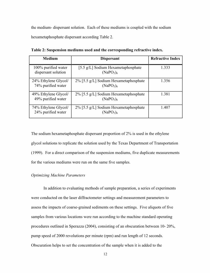
the medium- dispersant solution. Each of these mediums is coupled with the sodium

hexametaphosphate dispersant according Table 2.

Table 2: Suspension mediums used and the corresponding refractive index.

Medium Dispersant Refractive Index

100% purified water dispersant solution

[5.5 g/L] Sodium Hexametaphosphate (NaPO3)6

1.333

24% Ethylene Glycol/ 74% purified water

2% [5.5 g/L] Sodium Hexametaphosphate (NaPO3)6

1.356

49% Ethylene Glycol/ 49% purified water

2% [5.5 g/L] Sodium Hexametaphosphate (NaPO3)6

1.381

74% Ethylene Glycol/ 24% purified water

2% [5.5 g/L] Sodium Hexametaphosphate (NaPO3)6

1.407

The sodium hexametaphosphate dispersant proportion of 2% is used in the ethylene

glycol solutions to replicate the solution used by the Texas Department of Transportation

(1999). For a direct comparison of the suspension mediums, five duplicate measurements

for the various mediums were run on the same five samples.

Optimizing Machine Parameters

In addition to evaluating methods of sample preparation, a series of experiments

were conducted on the laser diffractometer settings and measurement parameters to

assess the impacts of coarse-grained sediments on these settings. Five aliquots of five

samples from various locations were run according to the machine standard operating

procedures outlined in Sperazza (2004), consisting of an obscuration between 10- 20%,

pump speed of 2000 revolutions per minute (rpm) and run length of 12 seconds.

Obscuration helps to set the concentration of the sample when it is added to the

 

13  

dispersant (Malvern Mastersizer Manual, 1997). It is a measure of the amount of laser

light lost due to the introduction of the sample within the analyzer beam (Malvern

Mastersizer Manual, 1997). These machine parameters were varied through a series of

experiments that modified the obscuration of the laser beam, the speed of the pump and

the length of time of the analyses. The refractive index of the sediment and the degree of

absorption of the laser by the sediment were not altered as they were in the previous

study by Sperazza (2004) since it was concluded that the index of refraction has little

impact over the range for natural sediments, if absorption is properly set. Absorption

value accounts for the attenuation of light as it passes through the particle (Malvern

Mastersizer Manual, 1997). Absorption values were set at 1 for all experiments

according to the optimal values reported in Sperazza (2004). The absorption value is set

in the software, before an analysis by selecting “measure” à “manual measurement” à

“options” à “select sample material”, here a pre-cataloged material from the “material

list” can be selected or “add new” can be selected where the user can enter the absorption

value for the material being analyzed.

Obscuration- The degree of obscuration is representative of the amount of sample

in the suspension. Malvern Instruments recommends an acceptable range for obscuration

to be between 10 to 20 percent. In order to determine the optimal range of obscuration

values for coarse-grained particles, obscuration was varied in two ways: “addition” and

“dilution.” First, an addition approach was taken to alter the obscuration. The degree of

obscuration was varied in increments of about (as close to) 1 percent by adding sample

by pipette directly into the measurement beaker to achieve a range from ~1 to ~45

percent. Second, a high concentration suspension was made in the measurement beaker

 

14  

with a starting obscuration of ~45 percent. The first sample tested was over this range,

while the other two samples were tested over a range of ~1 to ~30 percent due to the

stress that the first sample put on the machine. This was decreased by adding additional

suspension medium with a pipette (deionized water with sodium hexametaphosphate

5.5g/l concentrated solution) to the beaker so that the degree of obscuration would

incrementally reduce by about ~1% with each addition until ~1% obscuration was

achieved. For both the addition and dilution methods of altering the obscuration, five

replicate analyses were conducted on three samples.

Pump Speed- The Hydro 2000 MU pump accessory unit has variable speed

settings that can be adjusted to accommodate particles of various sizes and densities. The

pump speed experiments were conducted by measuring an aliquot of sample over a range

of revolutions per minute (rpm) values without removing the measurement beaker. The

five samples varied in density, from 2.18 g/mL for the quartz rich sands to 3.60 g/mL for

the heavy mineral assemblage sand lag deposits. Five aliquots of each sample were run

over a pump speed ranging from 1000 rpm to 3000 rpm at increments of 100 rpm in a

600 mL beaker with 500 mL of medium in order to isolate the effects of pump speed on

measurement data. The mediums used in the experiments were the 5.5 g/l sodium

hexametaphosphate solution, 24%, 49% and 74% glycol solutions.

Measurement Duration- The Malvern Mastersizer 2000 takes 1000 measurement

snaps per second of the sediment. In order to optimize the length of time of the sample

analysis run, the time was varied from 1 to 30 seconds. This will vary the amount of

snaps in the measurement from 1,000 snaps to 30,000 snaps per measurement. Grain size

runs in this variable analysis are reported as the average of three successive runs, a total

 

15  

of 3,000 to 90,000 snaps being considered. The time was varied on five aliquots of the

five samples suspended in each of the various mediums in 1-second increments without

removing the measurement beaker in order to find the optimal length of run time for

coarse grain size analysis.

Results and Discussion

Subsampling and Aliquot Introduction

Dry sieving the sample before subsampling is a necessary sample preparation step

when working with sand sized sediments. Grains larger than 1.5 millimeters may not

pass through the Hydro 2000 MU pump and particles may get lodged in the propeller,

jamming the pump. The preliminary dry sieving of the sample did not skew the results in

the target grain size range and larger particles are recovered for use, if needed, in the

study. Of the five samples, only two had grains larger than 1.4 mm, these were <1% of

the bulk sample mass of those two samples, the Goldsmith Microfault and Napeague

sands.

Of the two aliquot introduction techniques, both proved to have high

reproducibility in the results and show no distinct differences in the reported grain sizes

(Figure 5). The dried method could result in adding too much sample initially and having

to lower the obscuration percent later on by diluting the suspension. After applying the

minute of sonication with the pump accessory, some samples show an increase in

obscuration value due to the dispersion of finer grains stuck onto the coarser grains. For

this reason, the pipette method is preferred because it allows the sample aliquot to be

introduced into the measurement beaker in a controlled manor.

 

16  

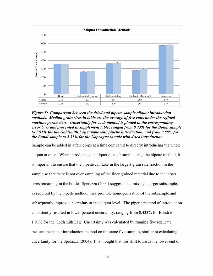
Figure 5: Comparison between the dried and pipette sample aliquot introduction methods. Median grain sizes in table are the average of five runs under the refined machine parameters. Uncertainty for each method is plotted in the corresponding error bars and presented in supplement table; ranged from 0.43% for the Bondi sample to 1.91% for the Goldsmith Lag sample with pipette introduction, and from 0.88% for the Bondi sample to 2.31% for the Napeague sample with dried introduction.

Sample can be added in a few drops at a time compared to directly introducing the whole

aliquot at once. When introducing an aliquot of a subsample using the pipette method, it

is important to ensure that the pipette can take in the largest grain size fraction in the

sample so that there is not over sampling of the finer grained material due to the larger

sizes remaining in the bottle. Sperazza (2004) suggests that mixing a larger subsample,

as required by the pipette method, may promote homogenization of the subsample and

subsequently improve uncertainty at the aliquot level. The pipette method of introduction

consistently resulted in lower percent uncertainty, ranging from 0.433% for Bondi to

1.91% for the Goldsmith Lag. Uncertainty was calculated by running five replicate

measurements per introduction method on the same five samples, similar to calculating

uncertainty for the Sperazza (2004). It is thought that this shift towards the lower end of

Bondi Goldsmith Crossbed Goldsmith Lag Goldsmith MicroFault Napeague Dried 355 267 364 280 577 Pipette 354 270 370 301 583

0

100

200

300

400

500

600

700 M

edia

n G

rain

Siz

e (µ

m)

Aliquot Introduction Methods

 

17  

uncertainties is due to the homogenization of the subsample through this method. The

dried method may be more susceptible to preferentially selecting grains of certain sizes

and/ or densities based on sample settling in the bulk sample when creating the

subsamples and aliquots.

Dispersant and Medium

The chemical dispersant used in all experiments was sodium hexametaphosphate

(TxDOT, 1999; TYNER, 1939; TCHILLINGARIAN, 1952; ROYCE, 1970). This was used in a

solution of purified water to disperse small grains and prevent grains from aggregating

after the one minute of sonication. The initial volume of suspension medium for the

particle size analysis was 500 mL of the 5.5 g/l sodium hexametaphosphate solution.

Additional experimental mediums included varying amounts of ethylene glycol were

measured according to the standard operating procedures established by the Texas

Department of Transportation (TxDOT), in Tex-238-F. The Texas Department of

Transportation hypothesis was that the higher viscosity of the glycol might better suspend

the particles than the water and chemical dispersant solution. The results from the series

of experiments showed that the suspension medium has insignificant effect on the grain

size results, aside from the 74% glycol solution which resulted in consistently lower

median grain sizes and had increased associated error. A more viscous medium does not

significantly enhance the suspended particles when compared to the 5.5 g/l sodium

hexametaphosphate and water solution (Figure 6). At higher concentrations of the

ethylene glycol solutions, the Malvern Mastersizer 2000 encountered problems with the

cell being “wet” or “dirty” and measurements were unable to be completed. The machine

had to be flushed with bleach to effectively clean the cell windows for measurement.

 

18  

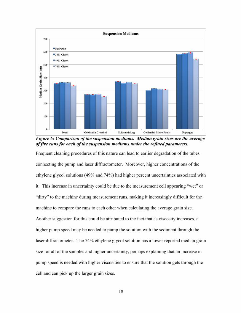
Figure 6: Comparison of the suspension mediums. Median grain sizes are the average of five runs for each of the suspension mediums under the refined parameters.

Frequent cleaning procedures of this nature can lead to earlier degradation of the tubes

connecting the pump and laser diffractometer. Moreover, higher concentrations of the

ethylene glycol solutions (49% and 74%) had higher percent uncertainties associated with

it. This increase in uncertainty could be due to the measurement cell appearing “wet” or

“dirty” to the machine during measurement runs, making it increasingly difficult for the

machine to compare the runs to each other when calculating the average grain size.

Another suggestion for this could be attributed to the fact that as viscosity increases, a

higher pump speed may be needed to pump the solution with the sediment through the

laser diffractometer. The 74% ethylene glycol solution has a lower reported median grain

size for all of the samples and higher uncertainty, perhaps explaining that an increase in

pump speed is needed with higher viscosities to ensure that the solution gets through the

cell and can pick up the larger grain sizes.

0

100

200

300

400

500

600

700

Bondi Goldsmith Crossbed Goldsmith Lag Goldsmith Micro Faults Napeague

Med

ian

Gra

in S

ize

(µm

)

Suspension Mediums

Na(PO3)6

24% Glycol

49% Glycol

74% Glycol

 

19  

Obscuration

Optimal obscuration occurs when a sufficient number of suspended particles are

present to significantly diffract the laser beam but the suspension is not so dense that the

laser light cannot penetrate the suspension. The effect of obscuration on sand sized

particles was tested over a range from ~1 to ~45 percent obscuration. The results show

that below 8% and above 28% obscuration reported median grain size has high

variability. Experimental results are stable between 16 to 24 percent obscuration (Figure

7). This is consistent with the results found for very fine-grained materials, 10-50 µm, in

Sperazza (2004), where the range of 15 to 20 percent was adopted as the target for the

standard operating procedure. When obscuration values were >35% the pump accessory

was being stressed and became jammed a few times. This is due to the amount of

material that was in the measurement beaker to achieve a high obscuration value. For

this reason, obscuration analyses were only run on samples in the purified water and not

with the ethylene glycol suspension medium to reduce the risk of harming the pump.

Additionally, the obscuration was only analyzed on three samples, Goldsmith Crossbed

sands, Goldsmith Micro-Fault sands and Bondi Beach sands because of the strain that the

high amounts (about 45+ grams) of sediment required for this experimental test were

putting onto the pump. During these runs the pump would sound strained and was

experiencing some issues and I did not want to break the pump accessory. All samples

exhibited stability in both the addition and dilution analysis after about 15% obscuration.

Malvern recommends running the analysis at a lower obscuration for optimal results

(Malvern Mastersizer Manual, 1997). That recommendation is supported by these results

 

20  

and suggests that there is no need to run the obscuration at a level higher than what can

be handled by the pump accessory.

0 50

100

150

200

250

300

350

400

450

1 2

3 4

5 6

7 8

9 10

11

12 1

3 14

15

16 1

7 18

19

20 2

1 22

23

24 2

5 26

27

28 2

9 30

31

32 3

3 34

35

36 3

7 38

39

40 4

1 42

44

Median Grain Size (µm)

Perc

ent O

bscu

ratio

n

Obs

cura

tion

Gol

dsm

ith C

ross

bed A

dditi

on!

Gol

dsm

ith C

ross

bed

Dilu

tion!

Bond

i Add

ition!

Bond

i Dilu

tion!

Gol

dsm

ith M

icro

Faul

ts A

dditi

on!

Gol

smith

Mic

roFa

ults

Dilu

tion!

Fig

ure

7: M

edia

n gr

ain

size

s of t

he sa

mpl

e ve

rsus

per

cent

obs

cura

tion.

Run

s wer

e co

mpl

eted

at a

tim

e of

12

seco

nds,

cons

tant

pum

p sp

eed

and

vary

ing

perc

ent o

bscu

ratio

n fr

om ~

1-45

% fo

r the

firs

t sam

ple

and

~1-3

0% fo

r th

e re

mai

ning

two

sam

ples

. V

aryi

ng o

bscu

ratio

n by

add

ition

of n

ew sa

mpl

e an

d di

lutio

n of

sam

ple

in m

easu

rem

ent

beak

er w

ere

test

ed o

n th

ree

sam

ples

.

 

 

21  

Pump Speed

The effect of pump speed on resultant grain size was examined through a series of

experiments with samples suspended in sodium hexametaphosphate solution and 49%

glycol. Sediments are suspended in the measurement beaker by turbulence created by the

Hydro 2000 pump accessory. This turbulence propels the suspension through a closed

system tube setup so that the suspension is driven through the measurement cell and

returned to the measurement beaker. When the samples were run under the standard

operating procedure pump speed of 2000 rpm, there was variability in the reported grain

sizes towards the coarser size fractions. The measurement cell was taken out of the laser

diffractometer and the pump was left continually running at pump speeds from 1000 rpm

to 3000 rpm so that the behavior of the sediments in the cell could be observed. At 2200

rpm, there were some grains that did not leave the measurement cell and circled around.

Additionally, some grains would slowly move downward in the cell rather than flowing

through. When the cell was removed and pump speed was running at 2600 rpm, all the

grains would flow smoothly through the measurement cell.

The analytical effect of variation in pump speed on median grain size was tested

experimentally from 1000 to 3000 rpm. The results showed that sand sized sediment

suspended in a 5.5 g/l sodium hexametaphosphate solution is stable between 2400 to

3000 rpm (Figure 8A). There is gradual variability in the samples between 2200 to 2400

rpm and high variability at pump speeds <2200 rpm. The coarse grained samples

suspended in the 49% water/ 49% glycol/ 2% sodium hexametaphosphate (TxDOT,

1999) medium are all stable between 2600 to 3000 rpm (Figure 8B). All but the coarsest

grained sample (median grain size ~600µm) are stable between 2300 to 3000 rpm.

 

22  

Figure 8: A-Median grain size of the samples versus pump speed with sediment suspended in the standard 5.5 g/l sodium hexametaphosphate (Na(PO3)6) and water solution. Runs were completed at a time of 12 seconds, obscuration held between 15-20% and varying pump speed. B- Median grain size of the samples versus pump speed suspended in a 49% glycol, 49% deionized water and 2% sodium hexametaphosphate (Na(PO3)6) solution. Runs were completed at a time of 12 seconds, obscuration between 15-20% and varying pump speed.

The experimental results for all samples show moderate variability between 1900 to 2200

rpm and significant variability <1900 rpm. At pump speeds nearing 3000 rpm, surface

0 !

100 !

200 !

300 !

400 !

500 !

600 !

700 !

800 !

1000!1100!1200!1300!1400!1500!1600!1700!1800!1900!2000!2100!2200!2300!2400!2500!2600!2700!2800!2900!3000!

Med

ian G

rain

Size

(µm

)

Pump Speed (rpm)!

Pump Speed-Sodium Hexametaphosphate!

0!

100!

200!

300!

400!

500!

600!

700!

800!

1000!1100!1200!1300!1400!1500!1600!1700!1800!1900!2000!2100!2200!2300!2400!2500!2600!2700!2800!2900!3000!

Med

ian

Gra

in S

ize

(µm

)!

Pump Speed (rpm)!

Pump Speed- 49% Glycol!

Bondi!

Goldsmith Microfaults!

Goldsmith Crossbed!

Goldsmith Lag!

Napeague!

! A!

B!

 

23  

turbulence was dramatically increased, which could result in the introduction of air

bubbles to the measurement beaker, leading to erroneous results. Based on these

observations and experimental results a pump speed of 2600 rpm was selected as the

optimum and was used in the other experimental measurements in this study. All

samples in all mediums showed stability at this pump speed.

Measurement Duration

With time, there is a chance to have greater variability in the reported grain sizes

due to the increased heterogeneity in samples that are moderately or poorly sorted. The

Malvern Mastersizer 2000 and pump accessory work in a closed system so that the

suspension that is carried through the measurement cell is continuously being circulated

around. The objective of this parameter was to find an optimal length of time for

measurements to accurately analyze the grain size representative of all suspended

particles. The Malvern instrument takes 1,000 data snaps per second with three

consecutive runs, the software then computes the averages of these runs to give a final

grain size report. The length of time for each run was varied from 1 to 30 seconds in 1-

second increments. All grain size measurements were stable between 7 to 17 seconds

(Figure 9). There was a slight variability <7 seconds and >17 seconds in some samples.

The variability at the shorter times is most likely attributed to not having enough time to

fully represent the aliquot in the suspension. Variation at the longer times was a slight,

but gradual increase in grain size, this could be due to finer grained particles adhering to

coarser grains as a nucleus, causing them to be represented as larger. It is recognized that

the 30-second duration provides a higher number of counts, and accordingly, lower

uncertainty. However, since the results are stable over time and the method seeks to

 

24  

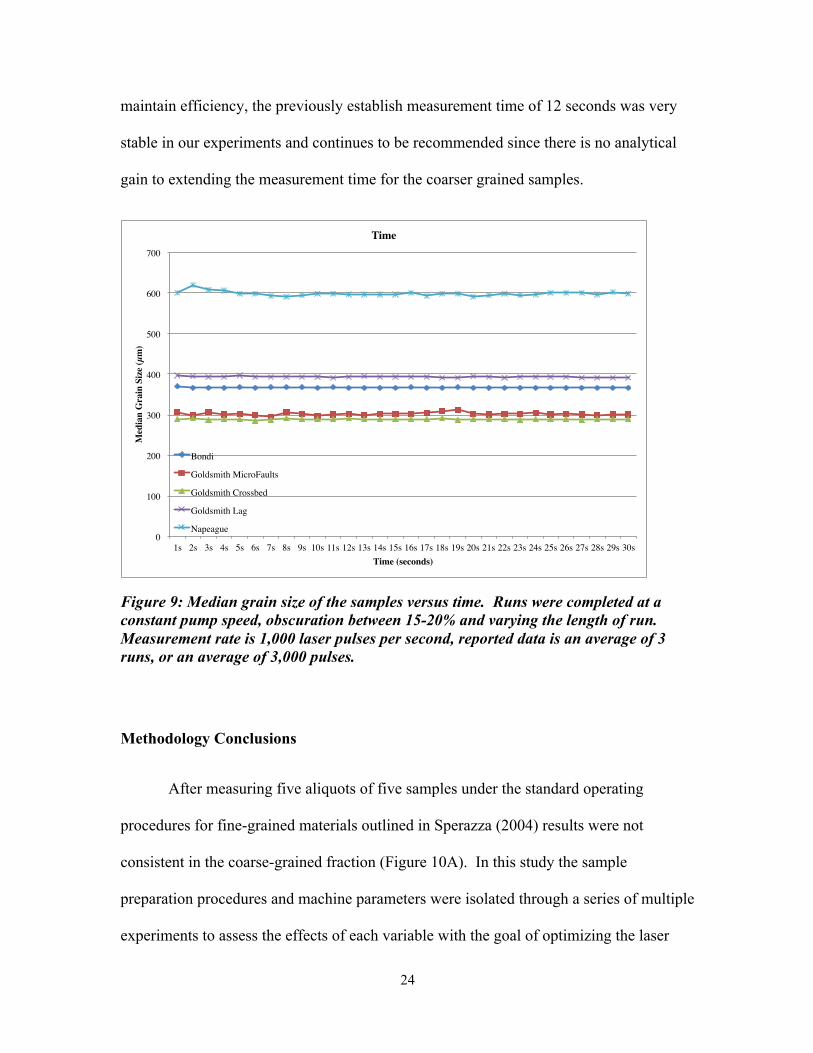
maintain efficiency, the previously establish measurement time of 12 seconds was very

stable in our experiments and continues to be recommended since there is no analytical

gain to extending the measurement time for the coarser grained samples.

Figure 9: Median grain size of the samples versus time. Runs were completed at a constant pump speed, obscuration between 15-20% and varying the length of run. Measurement rate is 1,000 laser pulses per second, reported data is an average of 3 runs, or an average of 3,000 pulses.

Methodology Conclusions

After measuring five aliquots of five samples under the standard operating

procedures for fine-grained materials outlined in Sperazza (2004) results were not

consistent in the coarse-grained fraction (Figure 10A). In this study the sample

preparation procedures and machine parameters were isolated through a series of multiple

experiments to assess the effects of each variable with the goal of optimizing the laser

0 !

100 !

200 !

300 !

400 !

500 !

600 !

700 !

1s! 2s! 3s! 4s! 5s! 6s! 7s! 8s! 9s! 10s!11s!12s!13s!14s!15s!16s!17s!18s!19s!20s!21s!22s!23s!24s!25s!26s!27s!28s!29s!30s!

Med

ian

Gra

in S

ize

(µm

)!

Time (seconds)!

Time!

Bondi!

Goldsmith MicroFaults!

Goldsmith Crossbed!

Goldsmith Lag!

Napeague!

 

25  

diffraction techniques for coarser grained, sand sized, sediments. The experimental

design was modeled after the design for fine grained sediment conducted in Sperazza

(2004). Results are summarized in Table 3.

Table 3: Summary of the experimental results from this study.

         

 Sample  

Preparation  

Target  Test   Tested  Range  

Analytical  Impact   Impact  compared  to  fine-­‐  grained  parameters  

Refined  Standard  Operating  Procedure  

Sieve   No  sieve  vs.  1.4mm  

Particles>1.45mm  have  the  potential  to  jam  the  pump  accessory  and  not  be  introduced  to  the  measurement  cell.  

High   Dry  sieve  at  1.4mm  

Aliquot  Introduction  

Dried  vs.  Pipette  

No  significant  difference  in  results  dependent  on  introduction  method.  

Low   Pipette  

Suspension  Medium  

Na(PO3)6  24%  glycol  49%  glycol  74%  glycol  

No  significant  difference  in  results  between  the  mediums,  except  with  the  74%  glycol  solution.  

Low   Na(PO3)6    

     

Machine  Parameter  

Obscuration   1-­‐45%   Stable  between  15  to  24%.  High  variability  <8%  and  >28%.  

Medium   15-­‐20%  

Pump  Speed   1000-­‐    3000  RPM  

Stable  between  2400  to  3000  RPM.  Gradual  variability  between  2200  to  2400  RPM.  High  variability  <2200  RPM.  

High   2600  RPM  

Length  of  Run   1-­‐30  seconds  

Stable  between  7  to  17  seconds.  Slight  variability  <7  and  >17  seconds  in  some  samples.  

Low   12  seconds  

Sample preparation for coarse grained sediments involved the addition of dry

sieving the bulk sample first before subsampling to separate out any grains (>1.4 mm)

that might not be able to pass through the Hydro 2000 MU pump. Two methods of

aliquot introduction were tested, the dried and pipette, with no dramatic variation in the

reported grain size. The pipette method is preferred, when sample lamina are not

preserved, because sample introduction can be better controlled and allow for the proper

 

26  

obscuration range to be achieved more efficiently. If lamina are present in the sample,

and the difference between the lamina would be of interest, it is recommended to directly

sample from each lamina and introduce through the dried method to prevent mixing of

the lamina. Moreover, a larger subsample is mixed with the dispersant and may improve

uncertainty at the aliquot level by promoting homogenization of the subsample. This is

supported by the lower uncertainties associated with the pipette introduction method.

The only sample with a slightly higher uncertainty with the pipette introduction method is

the Goldsmith Lag sample. This could be attributed to the increased density of the

heavier mineral assemblage of this sample, causing some loss of sample when extracting

the pipette from the sample jar.

The chemical dispersant used throughout the experiments was the sodium

hexametaphosphate; this is commonly used in various studies (TYNER, 1939;

TCHILLINGARIAN, 1952; ROYCE, 1970). This was tested against a more viscous fluid,

ethylene glycol, used by the Texas Department of Transportation. Glycol concentrations

of 24%, 49% and 74% were tested but did not improve experimental results or reduce the

need for higher pump speeds. It is recommended to use the 5.5 g/l sodium

hexametaphosphate and water solution for sample dispersant and suspension medium.

The optical parameters of the machine were not adjusted in this study because the

naturally occurring sediments utilized have similar mineralogy to those measured in the

previous study. Sperazza (2004) goes into extensive detail on the effects of absorption

and index of refraction on laser diffraction measurements. The parameters isolated and

analyzed in this study were the obscuration, pump speed, and length of run time. When

compared to the fine-grained parameters, altering the length of run time had minimal

 

27  

effect on coarse-grained material and the obscuration had a slight effect on the reported

grain size. With coarse-grained sediment it is important to keep the obscuration in the 15

to 25% range. Exceeding this amount can result in having too much sediment sample in

the measurement beaker, which can strain the pump. Below this range, there may not be

enough sediment particles suspended in the measurement cell to sufficiently diffract the

laser beam. Experiments on these parameters confirm the previously suggested values,

obscuration between 15 to 20% and a run time of 12 seconds. Isolating the pump speed

variable had a significant impact on reported coarse grain size compared to the fine-

grained parameters. In this study we have shown that the variable results from running

the coarse grained materials under the fine-grained standard operating procedures were

attributed mainly to the pump speed used. To observe this, the cell was taken out of the

laser diffractometer while pumping the suspension through at various pump speeds. At

lower pump speeds, 1000 to 2200 rpm, sediment particles were not making their way

through the measurement cell. At lower pump speeds, 1000 to 1700 rpm, some sediment

was settling to the bottom of the measurement beaker and not being introduced through

the measurement cell for analysis. At pump speeds from 1000 to 2200 rpm, some

particles that were introduced into the measurement cell remained in the cell and slowly

circulated around in turbulence, this leads to simply oversampling of these larger

particles that did not have enough propulsion from the pump to move up through the cell

and exit. Moreover, some of the larger grains would slowly move downwards in the cell

along one axis. This type of behavior results in misrepresentation of the grain size and

result in a reported grain size that is coarser than the actual sediment size. Once

increasing the pump speed to 2300 rpm, stable and reproducible results in the samples

 

28  

with median grain size ~300 µm occurred. When the pump speed was increased to the

stable value of 2600 rpm and the cell was taken out for observation, all particles moved

linearly through the cell with no oversampling.

While the suspension medium, except for the 74% glycol solution, did not have

an impact on the reported grain size, a more viscous fluid (ex: glycol solution) can be

used as in TxDOT (1999) for coarse- grained materials, but is not necessary for improved

or optimal results. The change in solution viscosity did not change the recommendation

of the 2600 rpm pump speed. It is important to note, that a solution that deviates from

about ~50% water can cause the laser diffraction cell to appear “wet” or “dirty” and that

this problem is alleviated by rinsing the diffractometer with a bleach solution. This

treatment of the machine can lead to premature degradation of machine tubing and

excessive cell cleaning. For this reason, it is recommended to continue to run grain size

analysis in the 5.5 g/l sodium hexametaphosphate and water solution.

The comparison between the reported grain sizes using the previous methods and

the refined methodology, summarized in Table 3, is shown in Figure 10A&B. It is

important to note that there is no longer the inconsistency between the three measurement

analyses and the average in the coarse-grained fraction, rather, there is one tight curve

showing the low error and increased accuracy of the method (Figure 10B). Laser-

diffraction on coarse-grained sediment varies from fine-grained sediment in that a sample

preparation step of dry bulk sieving the sample at 1.4 mm is required so that the pump

does not become jammed. The revised machine parameters for laser diffraction of

naturally occurring coarse-grained sediment require an increase in pump speed to 2600

rpm from 2000 rpm, while maintaining an obscuration of between 15 to 20% and a

 

29  

measurement time of 12 seconds.

Figure 10: Comparison of the reported grain sizes of the same sample run under the methods outlined in Sperazza et. al., 2004 and the refined methods. The previous standard operating procedures (A) correspond to a pump speed of 2000 rpm and analysis time of 12 seconds, keeping obscuration between 10-20%. Refined parameters (B) have a recommended pump speed of 2600 rpm, 12 second analysis time and obscuration between 15-20%. Following these refined parameters brings the three measurements and the average in line to a tight curve, with no variation in the coarse-grained fraction. Average associated uncertainty went from 6.16% to 1.27%.

 

30  

These refined sample preparation techniques and machine parameters yield grain

size analysis results that can be reproduced with high levels of confidence and

uncertainty of ~1.7% at 2 sigma. The uncertainty analysis was focused on the median

grain size measurement, D50. Uncertainty is used as a measure of precision and is

calculated at the 95% confidence interval. To quantify the overall uncertainty, 7 samples

(five of which were used throughout this methods study as well as two additional

samples) were run through 7 replicate analysis under the refined parameters derived in

this study (Table 3). The equation used to calculate uncertainty at the 95% confidence

interval is:

Microsoft Excel was used to build the formula and calculate the various parameters using

the build in statistical functions. The highest calculated uncertainty associated with a

sample is reported. It is important to note that the samples used in this methods study are

all mono-modal. A bimodal or polymodal distribution will have different total

uncertainties associated with the distribution. For example, a larger percent volume of

fine grains will have more uncertainty associated with the ninethieth percentile, D90, then

the tenth percentile.

Careful application of the techniques must be ensured since error can be

introduced through variations in sample preparation procedures, machine settings and

parameters. It has been suggested that another possible source of error could be the

optical properties associated with the diverse mineral compositions of naturally occurring

 

31  

sediments. However, this study tested a variety of sands with different compositions and

the absorption value was set at 1 for all of the measurements. This study has shown that

laser diffraction can measure sand sized sediments quickly, with high reproducibility and

without the need for extensive mineralogical determinations. Such precision and

efficiency makes possible a new generation of sedimentologic studies where subtle

changes in grain size on small scales can be analyzed and used to infer changes in barrier

island environments and subenvironments.

 

32  

Chapter 3

Grain Size as a Proxy of Depositional Environment Through Assessment of

Sediment Cores from Kismet, Fire Island, New York

Study Area

Fire Island is a barrier island located south of the terminal moraine of the

Laurentian ice sheet, which began its retreat about 8,000-12,000 years ago (SCHWAB, et

al., 2000; SCHUBERT, 2009). The island is 32 miles long and averages less than half a

mile wide. It is below the southern coast of Long Island and separates Great South Bay

and Moriches Bay from the Atlantic Ocean. Barrier island beaches are similar to

mainland beaches but are separated from land by a shallow lagoon, estuary or marsh and

are commonly dissected by tidal channels or inlets (PIERCE AND COLQUHOUN, 1970 and

RIGGS, et al., 1995). The oldest part of the Fire Island barrier is in the center, near the

Watch Hill area (SCHWAB, et al., 2000; LEATHERMAN AND ALLEN, 1985; PANAGEOTOU

AND LEATHERMAN, 1986).

The study area is located approximately 13 miles West of Watch Hill and is in an

area where barrier island transgression is much less rapid compared to the Eastern most

parts of the barrier island system (SCHWAB et al., 2000). Beach, dune and aeolian or

backbarrier flat environments are well developed here. It is hoped that a study of the

modern deposits will serve as an aid in distinguishing similar environments in older

sediments. To complete the field-work, a permit was obtained from the National Park

Service and five sediment cores were collected in a shoreline normal transect (Figure 11).

Additionally, grab samples of the surface sediments were collected laterally from the core

 

33  

locations at increments of 0.5 and 1 meter to both sides corresponding to the dune, beach

(sand and lag deposits) and aeolian flat or backbarrier environments.

Figure 11: The location of the study area on Fire Island and a close up of the shoreline normal transect along which the sediment cores were taken. The first core, A was taken closer to the ocean beach, B1 and B2 in the middle of the island and C1 and C2 were taken from the bay side.

Methods

When collecting the sediment cores it is important to maintain the stratigraphy

and a simple auger or push core is not sufficient, as these methods will disturb the

stratigraphic relationships of the sediments. Vibracoring is a subsurface sediment

acquisition technique (PIERCE AND HOWARD, 1969; HOWARD AND FREY, 1975; DREHER

et al., 2008; BISHOP et al., 2011) that returns sediment preserved within its stratigraphic

!

Kismet!A1!

Kismet!B1&2!

Kismet!C1&2!

 

34  

and sedimentologic context. Cores are measured for grain size with depth and

stratigraphy is assessed visually.

Core Collection

The cores are collected through the vibracoring method using Hofstra

University’s vibracore system. Vibracoring is a technique for collecting unconsolidated

sediments and works by combining gravity and high frequency vibration to penetrate the

substrate. In general, the frequency of vibrations is in the range of 3,000 to 11,000

vibrations per minute (vpm) and the amplitude of movement is on the order of a few

millimeters. As a result, the vibrations cause a thin layer of sediment to mobilize along

the inner and outer tube wall, which reduces the friction along the core but also causes 1-

2 millimeters of disturbance on the edges of the core. This is minor when analyzing the

core since the core diameter is 7.62 centimeters (3 inches) across. The coring methods

followed involve sharpening the bottom end of the core pipe to enhance the ability of the

pipe to cut through plants and roots before penetrating unconsolidated sands with a 7.62

centimeter diameter aluminum irrigation pipe driven into the subsurface. Approximately

two and a half meter (eight feet) long sections of pipe are oriented vertically to the

substrate surface and driven by hand a few centimeters into the sediment. A cement-

vibrating machine is clamped to the pipe along with several lengths of rope used to guide

the pipe downward after the vibrating machine is started up. The cement-vibrating

machine is gasoline powered and resembles a lawnmower engine attached to a small

wheelbarrow. A cable and vibrating head are attached to the engine with U-bolts. The

downward force supplied by pulling on the ropes paired with the vibrations mobilizes the

sediments that come in direct contact with the pipe allowing it to penetrate (Figure 12).

 

35  

Prior to removal, a cap is secured on the top of the core pipe to create a suction seal as the

core is pulled upward from the ground.

The core is removed from the subsurface using a hand-operated farm jack and ropes to

pull the core up and out of the hole (Figure 13). The <10 centimeter diameter hole

remaining self sealed within minutes as the unconsolidated sediment along the sides

flows into the gap. Apart from a small area of trampled vegetation, disruption of the

coring sites was minimal.

When collecting sediment cores, it is important to account for the degree of

compaction. Compaction was measured in the sediment cores at maximum penetration

depth when the vibracore no longer penetrates the substrate and drilling ceases. The

depth from the top of the core barrel to the top of the sediment surface inside the pipe is

measured, the length of the pipe remaining above the ground is measured and former is

Figure 12: (Top) The sediment core is being drilled into the ground by the power from the motor and the downward force of three ropes, evenly spaced around the sediment core.

Figure 13: (Bottom) The vibracore has been capped and is being pulled upward by a farm jack.

 

36  

subtracted from the latter to determine compaction of sediment inside the core barrel

(Bishop, et al., 2011). The equation used for compaction is as follows:

Compaction = (Depth to Top of Sediment Inside Pipe) – (Length of Pipe Above Ground)

In order to analyze the sediment cores, they had to be split. Splitting methods

consisted of marking the top and bottom of the cores at 0O and 180O with a circular

protractor to ensure that they were spilt exactly in half. Then a line connecting the top

and bottom marks was drawn with a tape measure as a guide. Using electric scissors, the

core was cut along one of these lines and then taped along the cut so that the other side

could be cut with the scissor. Once both sides were cut, a large knife was used to slice

the core in half. The knife was not slid down the length of the core as not to disturb the

sediments or stratigraphy. The core was allowed to separate into halves along natural

breaks but when necessary, the knife was inserted into the core and gently pulled out in a

stabbing or cutting motion. Photographs of the cores were taken before any analyses

were done (Figure 14).

Visual Description

The sediment cores were described on a centimeter scale basis through visual

descriptions and microscope analysis. All cores were described for sediment type, color,

mineralogy, abruptness of contact between distinct sedimentary deposits and grain size

similar to the vibracore description method in Scileppi and Donnelly (2007). The

mineralogy was completed through microscope analysis and was completed for each of

the visually distinct sedimentary deposits. This data provides an additional qualitative

description of the sediments preserved in each of the cores. Grain-size analysis was

conducted using a Malvern Mastersizer 2000. Grain size provides a quantitative

 

37  

description of the preserved sediments in addition to being used in a proxy development

of depositional environment and barrier island facies.

0!

10!

20!

30!

40!

50!

60!

70!

80!

90!

100!

110!

120!

130!

140!

150! A+

!C2! 0!

10!

20!

30!

40!

50!

60!

70!

80!

90!

100!

C2

C1

B1

Figure 14: Photograph of all of the sediment cores taken, except for core B2, which was 30 centimeters of unconsolidated dune sands and plants.

 

 

38  

Typical barrier beach sediment consists of well-sorted and rounded sand

(SCILEPPI AND DONNELLY, 2007; BOGGS, 1995). Overwash deposits commonly have

sharp lower contacts, which indicate a sudden onset of high transport energy and, in some

cases, the erosion of substrate during the event (SCILEPPI AND DONNELLY, 2007;

DONNELLY et al., 2001b; DONNELLY AND WEBB, 2004). Dark, parallel laminations of

heavy minerals are common features of overwash deposits (SCHWARTZ, 1975; HENNESSY

AND ZARILLO, 1987). To summarize:

• Barrier beach sediment: well-sorted and rounded sand

• Overwash deposits: dark, heavy mineral, parallel laminations and sharp lower contacts

Grain-Size Analysis

Grain-size analysis was performed for the length of all cores at 1-centimeter

intervals. A tape measure was laid out along the core to ensure sampling accuracy at

each centimeter. The samples were subsampled from one half of the split core with a

microspatula. The core aliquot was then passed through the number 14, 1.4 mm mesh,

sieve. The material passing though this sieve is within the practical limit of the laser

diffractometer and put into a clean and labeled 30 mL sample container and filled with

20mL 5.5 g/L sodium hexametaphosphate solution. Every aliquot taken from each of the

cores passed through the 1.44mm sieve, except in a few instances when a twig, shell

fragment or sparse pebble sized grain was sieved out. Each sample aliquot was between

5.0 to 10.0 grams. Sample mass was variable depending on the obscuration reading from

the Malvern Mastersizer 2000. The finer grained samples required a lower mass of

sample than the coarser grained sands. This difference is due to the particle density per

 

39  

weight of sample; finer sands have more particles per gram than coarser sands to

sufficiently diffract the laser beams. Obscuration was kept between 15-20% for all

samples; this is within the range of 10-20% obscuration as recommended by the results of

the methodology studies (DIAS AND SPERAZZA, 2012; DIAS AND SPERAZZA, 2013;

SPERAZZA et al., 2004). After sitting in the solution for a minimum of 24 hours, the

samples were first agitated with the VWR Analog Vortex Mixer, then pipetted into the

measurement beaker filled with 500mL sodium hexametaphosphate for analysis via the

laser diffractometer. After adding the sample to the measurement beaker, ultrasonication

was run through the Hydro 2000 MU pump accessory for one minute. According to the

refined methodology aforementioned, pump speed for analysis was set to 2600 rpm and a

measurement length of 12 seconds. The calculated particle size distribution is an average

of three, 12-second measurement runs. The median grain size, D50, from this average is

used in the statistical analyses.

Statistical Analysis

Grain-size data was exported as a text file from the Malvern Mastersizer software

and imported to Microsoft Excel for statistical analysis. Grain size has been used to

distinguish between beach, barrier-flat and dune facies (SIMMS, et. al., 2006). Mason and

Folk (1958) used statistical analysis of grain size data to differentiate between the beach,

dune and aeolan flat environments of a barrier island off of the Texas Gulf Coast. This

study will statistically analyze the grain size data for skewness, the third moment, as well

as calculate the fourth moment of the data, kurtosis (HAZEWINKEL, 1993; PROKHOROV,

1990). The statistical parameters will each be plotted against the median grain size.

According to Simms (2006) populations are best found and distinguished by a plot of

 

40  

skewness versus mean. A new method of recognizing clusters in the grain size data is

introduced in this study, K-means clustering. K-means is widely used to recognize

clusters in data sets in data mining, social sciences and survey data but has not been used

to look at clustering in facies modeling.

Skewness is often used in statistical analysis to see if the data from a distribution

is sound (DOANE AND SEWARD, 2011; YULE AND KENDALL, 1950). Statistically,

skewness measures the degree of asymmetry of a distribution; the skewness of a normal

distribution, where mean = median = mode, is zero since a normal distribution is

symmetric (DOANE AND SEWARD, 2011; ARNOLD AND GROENEVELD, 1995). A positive

skewness value indicates a distribution with an asymmetric tail extending towards more

positive values, where Mean > Median > Mode (DOANE AND SEWARD, 2011; ARNOLD

AND GROENEVELD, 1995). Conversely, a negative skewness would have a tail extending

towards more negative values, and Mean < Median < Mode (DOANE AND SEWARD, 2011;

ARNOLD AND GROENEVELD, 1995). Values far from zero suggest a non-normal, or

skewed, population (DOANE AND SEWARD, 2011; RAYNER, et al., 1995). Mathematically,

skewness is represented by the following equation:

Microsoft Excel has a built in function located in the statistics catalogue to calculate the

skewness of a dataset, SKEW( ). This statistical function of Microsoft Excel was used

for all skewness calculations. Skewness was calculated for each centimeter increment

from all of the sediment cores. Additionally, skewness was calculated for the surface

grab samples, representing the modern, known barrier beach facies. A plot of skewness

 

41  

versus mean for all grain-size data obtained from cores and modern samples was then

generated as a simple X-Y Scatter Plot.

Kurtosis is similar to skewness as it is also a measure of the dataset’s central

tendency (BALANDA AND MACGILLIVRAY, 1988; GROENEVELD AND MEEDEN, 1984;

MARDIA, 1970). As skewness looks at if the data is concentrated towards the right or left

of a normal distribution, kurtosis looks at the peakedness of the data (BALANDA AND

MACGILLIVRAY, 1988). It tells us if the distribution is more peaked than the normal

distribution, meaning more items are clustered about the mode value, or if the distribution

is flat on top. The distributions can be classified as mesokurtic, leptokurtic or platykurtic

(KIM AND WHITE, 2004; BALANDA AND MACGILLIVRAY, 1988; GROENEVELD AND

MEEDEN, 1984; MARDIA, 1970). Mesokurtic is a normal distribution with a kurtosis

value around 0.5 (KIM AND WHITE, 2004). Leptokurtic distributions have kurtosis values

greater than 0.525 and are characterized by peaks that are thin and tall and have tails that

are thick and heavy (KIM AND WHITE, 2004; MARDIA, 1970). Platykurtic distributions

have a kurtosis value less than 0.475, the peaks are somewhat flat, lower than mesokurtic

distributions and the tails are slender (KIM AND WHITE, 2004; MARDIA, 1970).

Mathematically, kurtosis is represented by the equation:

Located in the statistics catalogue of Microsoft Excel is a function to calculate the

kurtosis of a datasest, KURT ( ). This function was used for all kurtosis calculations.

 

42  

The formula was applied to each centimeter increment from all of the core data as well as

for the modern samples. A plot of kurtosis versus median grain size was then generated.

An additional statistical approach was introduced to identify distinct populations

or clusters in the data. Clustering algorithms are generally used in an unsupervised

fashion where the algorithm is presented with a set of data instances that must be grouped

according to some notion of similarity (WAGSTAFF et. al., 2001). K-means clustering is a

method commonly used to automatically partition a data set into clusters (WAGSTAFF et.

al., 2001; HARTIGAN AND WONG, 1979). The aim of the K-means algorithm is to divide

M points in N dimensions into K clusters so that the within-cluster sum of squares is

minimized (HARTIGAN AND WONG, 1979). K-means clustering algorithm was applied to

each sediment cores’ average grain size per centimeter with depth as well as to all of the

core data with skewness. The following Visual Basic for Applications (VBA) macro for

Microsoft Excel written by Sheldon Neilson (2011) was used (Appendix).

In summary, the algorithm works by selecting k initial cluster centers and then

iteratively refining them (WAGSTAFF, et. al., 2001; HARTIGAN AND WONG, 1979). First

each instance is assigned to its closest cluster center (WAGSTAFF, et. al., 2001; HARTIGAN

AND WONG, 1979). Following, each cluster center is updated to be the mean of its

constituent instances (WAGSTAFF, et. al., 2001; HARTIGAN AND WONG, 1979). The

algorithm converges when there is no change in the assignment of instances to clusters

(WAGSTAFF, et. al., 2001) or when there is a K-partition of the sample with within-cluster

sum of squares which cannot be reduced by moving points from one cluster to the other

(HARTIGAN AND WONG, 1979). To achieve optimality, usually less than 10 iterations are

required (HARTIGAN AND WONG, 1979).

 

43  

Results and Discussion

Cores in this study contain generally similar stratigraphies, planar bedding with

distinct contacts between beds and are dominantly composed of sand units of varying

grain size and mineral assemblages. Sediment core A is the only core that exhibits cross

bedding stratigraphy (Figures 14 and 15) in addition to the planar bedding. Five classes

of sediment occur in the cores: quartz sand, heavy mineral sand, arkose sand, quartz or

arkose sand with heavy minerals and peat. In all cores the quartz sand and heavy mineral

sand deposits are well-rounded, well-sorted to very well sorted deposits and occur with a

sharp contact. The arkose sands, found only in the C cores (Figure 14) are sub-angular to

sub-rounded and are moderately sorted. The deposits with the mixing of heavy mineral

sands and quartz or arkose sands contain sparse pebble sized grains as well as twigs,

which were sieved out before grain size analysis. The only sediment core with

significant peat was sediment core A; small peat nodules were also found in core B1.

The peat was in the bottom 10 centimeters of the core and is a discontinuous layer with

fine-grained sediment mixed with fibrous peat nodules (Figures 14 and 15).

Sediment core A consisted of alternating layers between quartz and heavy mineral

assemblage sands as well as areas of combined quartz and heavy mineral sands (Figures

14 and 15). The middle portion of the core, about 35-70 centimeters, is dominated by

cross stratification as well as a relatively thick, 13 centimeter, pure heavy mineral sand

deposit (Figures 14 and 15). Core A also has three deposits of coarser sands that contain

some small pebbles, plant and shell fragments. The bottom of the core consists of a few

very thin, parallel heavy mineral laminations with a sharp contact between darker sands,

 

44  

possibly from organic matter, plant material, shell fragments and fibrous peat nodules

(Figure 15).

Sediment cores B1 and B2 consist primarily of quartz sands (Figure 14). Core B2

is entirely well-rounded, well-sorted, unconsolidated quartz sand with median grain size

ranging from 191 to 197 µm (micrometers). The entire length of the core, 30

centimeters, contained plant material throughout. Core B1 is nearly identical to B2 for

the top 19 centimeters. At 20 centimeters there is a slight change in color of the sands,

but they remain well-sorted, well-rounded quartz sands, plant material is also present

throughout the core until 51 centimeters. The core has a thin, <1 centimeter, heavy

mineral band at 57 to 58 centimeters and a small, fibrous peat nodule at 63 to 64

centimeters (Figure 14).

!

120!cm!

147!cm!

25!cm!

50!cm!

Figure 3 Figure 4 !

120!cm!

147!cm!

25!cm!

50!cm!

Figure 3 Figure 4

Figure 15: Sediment core A upper section showing cross bedding and possible storm deposit (Left). Bottom of sediment core A showing the very thin heavy mineral parallel laminations, sharp contact and discontinuous fibrous peat nodules (Right).

 

 

45  

Sediment cores C1 and C2 are composed of well-sorted, sub-angular to sub-

rounded feldspar and well-rounded quartz sands, with a transition to darker material near

the bottom of both cores (Figure 14). C1 has an iron oxidation band at 52 centimeters,

below this plant material is present and the sands appear darker in color, possibly from

organic matter (Figure 14). Core C2 has a 5-centimeter layer of plant matter near the top

of the core, from 13 to 17 centimeters (Figure 14). The entire length of the core has

arkose and quartz sands throughout. At 75 centimeters the core has a mixing of heavy

mineral sands with the quartz and arkose sands. The bottom of the core from 75 to 97

centimeters consists of this mixed arkose, quartz and heavy mineral sand. There are also

a few very thin, parallel laminations of heavy minerals within the mixed sands. From 84

to 90 centimeters small to large pebbles are present.

Grain size analysis completed at centimeter intervals for the sediment cores

ranged from 191 to 723 µm for sediment cores A, B1, B2, C1 and C2 (Figure 16).

Sediment core A consists of median grain sizes generally in the 400-500 µm with areas of

lower grain size, 305-341 µm, associated with the heavy mineral deposits. The coarsest

particle sizes, 532-600 µm, in this core seem to be associated with areas that show a

mixing of quartz and heavy minerals, twigs, some pebble size grains and larger shell

fragments. Sediment cores B1 and B2 consisted of the finest median grain sizes, 190 to

197 µm, in the entirety of B2 and the upper 20 centimeters of B1 before increasing for

about 10 centimeters to median grain size of upper to middle 200-micrometer sizes.

 

46  

Figure 16: Grain size taken at each centimeter and plotted with depth for all five of the sediment cores.

Sediment core B1 then dropped back to median grain size of 190 to 210 µm before

gradually increasing in grain size to 416 µm at the 51-centimeter mark, the bottom

portion of the core has grain sizes in the low 400 micrometers. There is a thin lag deposit

in this core at the 57 to 58 centimeter depth (Figure 14), which has a lower grain size, 330

µm, than the surrounding sediments, 420 µm range. Sediment cores C1 and C2 contain

the coarsest sediments with median grain sizes in the 600-700 µm range. Core C1

gradually decreases in grain size with depth, reaching a low of 580 µm in the last three

centimeters of the core. Core C2 decreases in grain size with depth for approximately 30

centimeters, before increasing again, it then the grain size decreases gradually for about

40 centimeters, then increases again. The lower 75 centimeters of this core have a

significant decrease in grain size and this is the region where the arkose and quartz sands

where mixed with the heavy mineral sands.

0!

20!

40!

60!

80!

100!

120!

140!

160!

0! 100! 200! 300! 400! 500! 600! 700! 800!

Dep

th (c

m)!

Median Grain Size (μm)!

Kismet Cores!Depth vs. Grain Size !

A" B1" B2" C1" C2"

 

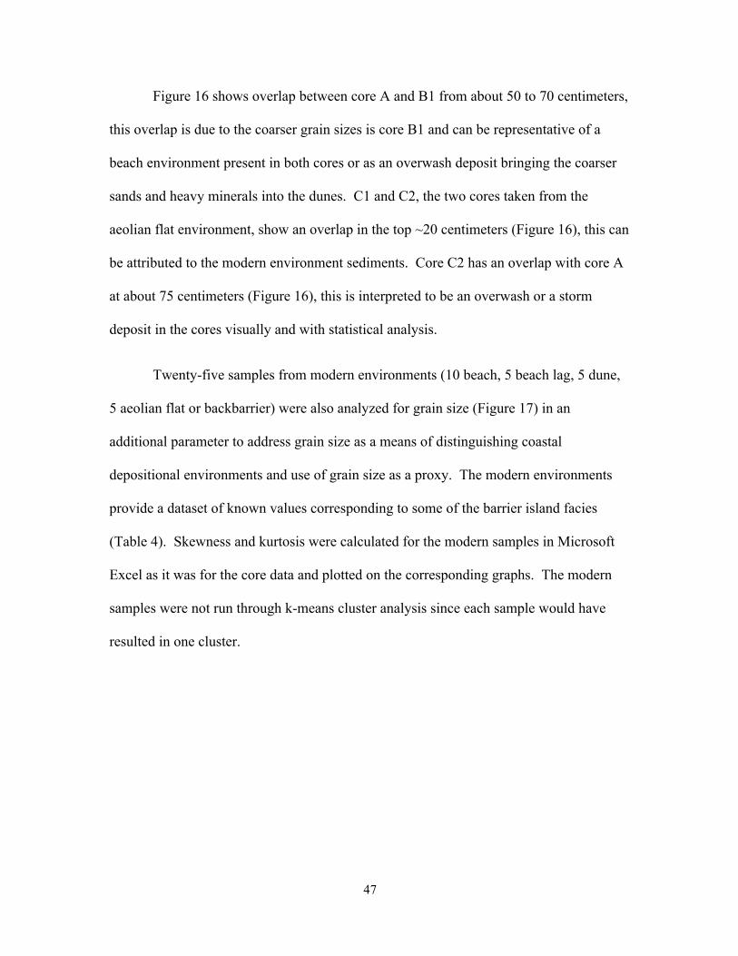
47  

Figure 16 shows overlap between core A and B1 from about 50 to 70 centimeters,

this overlap is due to the coarser grain sizes is core B1 and can be representative of a

beach environment present in both cores or as an overwash deposit bringing the coarser

sands and heavy minerals into the dunes. C1 and C2, the two cores taken from the

aeolian flat environment, show an overlap in the top ~20 centimeters (Figure 16), this can

be attributed to the modern environment sediments. Core C2 has an overlap with core A

at about 75 centimeters (Figure 16), this is interpreted to be an overwash or a storm

deposit in the cores visually and with statistical analysis.

Twenty-five samples from modern environments (10 beach, 5 beach lag, 5 dune,

5 aeolian flat or backbarrier) were also analyzed for grain size (Figure 17) in an

additional parameter to address grain size as a means of distinguishing coastal

depositional environments and use of grain size as a proxy. The modern environments

provide a dataset of known values corresponding to some of the barrier island facies

(Table 4). Skewness and kurtosis were calculated for the modern samples in Microsoft

Excel as it was for the core data and plotted on the corresponding graphs. The modern

samples were not run through k-means cluster analysis since each sample would have

resulted in one cluster.

 

48  

Figure 17: Particle size distribution for the modern environments sampled. The dune sands had the lowest average grain size; followed by the beach lag then quartz sands and the aeolian flat sands had the coarsest average grain size.

When the grain size data is statistically analyzed, cluster patterns in the data are

recognized. Plotting the modern samples and core data on a scatterplot of skewness

verses median grain-size shows five distinct populations (Figure 18). Population 1

contains the dune facies. Populations 2 and 3 contain the beach facies, with population 2

containing the beach quartz sand deposits and population 3 containing the beach lag

deposits. Population 4 contains the aeolian flat or backbarrier deposits. Population 5 is

thought to be storm or washover deposits. The modern samples provide a depositional

environment comparison that aids in the interpretation for what environment the clusters

in the core data are from.

!

Beach Aeolian Flats

Lag

Dune

 

49  

Figure 18: Skewness plotted versus median grain size for the core data and modern environments. Five populations are visually recognized.

Directly comparing the results from this study to those found by Simms (2006)

for Mustang Island, TX show that there is no overlap or correlation between the data,

although both studies concluded that plotting skewness versus median grain size allows

for clusters in the data to be interpreted into facies. Simms (2006) was able to note two

distinct populations in the data representing the modern beaches and dunes (Population 1)

and the barrier flats (Population 2). This difference between the data can be attributed to

the fact that these studies were conducted on two different barrier island systems.

Mustang Island is in the Texas Gulf Coast whereas Fire Island is off the south shore of

Long Island and directly interacts with the Atlantic Ocean on the beach side.

-3!

-2!

-1!

0!

1!

2!

3!

0! 100! 200! 300! 400! 500! 600! 700! 800!

Skew

ness!

Median Grain Size (μm)!

Median Grain Size vs. Skewness!

Modern Dune! Modern Beach! Modern Lag! Modern Backbarrier! Core Data A1! Core Data B1! Core Data B2! Core Data C1! Core Data C2!

Population*5

*

Population*4

*

*Population*1*

Population*2*

Population*3*

 

50  

Figure 19: Direct comparison of the results from this study to results from Mustang Island, TX.

The coarser grain sizes seen in all of the facies when compared to Simms (2006) can be

due to the increased energies. Barrier islands are active environments, the differing

results between the two studies provides support that in depth studies need to be

conducted on each barrier island system to best understand the dynamics and that

conclusions from one island system cannot be simply applied to another. Another

possibility to explain the differences between the data could be how skewness was

calculated. Simms (2006) does not provide the equation used to calculate this statistical

parameter and skewness has been defined in multiple ways. The function in excel

corrects for small sample bias by multiplying by the ratio n/(n-2) (DOANE AND SEWARD,

2011; REMENYI, et. al., 2010; CARR, 2008). The correction increases the value if the

skewness is positive, and makes the value more negative if the skewness is negative.

0 1 2 3

0.5

1.0

1.5

2.0

2.5

-0.5

-1.0

-1.5

-2.0 Median Grain Size (Phi)

Skew

ness

Simms (2006) 1

2

Population 1

Population 2

Population 3

Population 4

Population 5 (?)

 

51  

With large samples, the correction is almost negligible but with small samples, the

correction is substantial (REMENYI, et. al., 2010; CARR, 2008). Additionally, Simms

(2006) analyzed grain size of the samples using a Malvern Mastersizer 2000 under the

standard operating procedures in Sperazza (2004). This study has shown that those

parameters need to be refined for sand sized sediment to eliminate inconsistency between

measurements in the coarser end of the particle size distribution and increase confidence

in the results. Perhaps re-running the samples under the refined methodology would

allow for differentiation between the beach and dune facies in Simms (2006) population

1. When comparing the sample density between the two studies, this study as a higher

number of samples than the previous study, which brings up the possibility that more

samples might aid in cluster recognition. Moreover, Simms (2006) completed grain size

analysis in 25-centimeter intervals for the sediment cores, this study analyzed the

sediment cores at centimeter intervals, perhaps the centimeter scale resolution aided in

differentiating between the barrier island facies for Kismet, Fire Island.

Simms (2006) was not able to say anything meaningful about the other statistical

parameters of the data from Mustang Island. When kurtosis was run on grain size data

from the cores, it is possible to see some clustering in the data, but not as apparent as in

the skewness plot (Figures 20 and 23). The ability to differentiate between the clusters in

the kurtosis plot might be due to the higher resolution achieved by the new methodology

as well as the number of samples analyzed. When the distribution about the normal,

skewness versus kurtosis, is plotted for the core data, no clusters are recognized (Figure

21).

 

52  

Figure 20: Kurtosis plotted versus median grain size for the core data and modern environments.

This lack of clusters can suggest that median grain size is an important characteristic of

the data that must be accounted for when plotting and interpreting for barrier island

facies. Skewness versus median grain size allows for better differentiating between

clusters than kurtosis versus median grain size. This result adds significance to

calculating and analyzing the skewness of the distribution.

Figure 21: Plot of the distribution of the data about the normal. No apparent clusters.

0

0.2

0.4

0.6

0.8

1

1.2

0 100 200 300 400 500 600 700 800

Kur

tosi

s

Median Grain Size (um)

Median Grain Size vs. Kurtosis

Modern Dune Modern Beach Modern Lag Modern Aeolian Flat Core Data A1

Core Data B1 Core Data B2 Core Data C1 Core Data C2

0

0.2

0.4

0.6

0.8

1

1.2

-3 -2 -1 0 1 2 3

Kur

tosi

s

Skewness

Skewness vs. Kurtosis

Modern Dune

Modern Beach

Modern Lag

Modern Aeolian Flat

Core Data A1

Core Data B1

Core Data B2

Core Data C1

Core Data C2

Population 1 Population 2 Population 3

 

53  

Figure 22: Plot of the results from k-means clustering algorithm run on the skewness and median grain size data. K-means recognized five distinct clusters in the data.

Figure 23: Plot of the results from k-means clustering algorithm run on the kurtosis and median grain size data. K-means recognizes three distinct clusters in the data.

Running the k-means clustering algorithm on the data resulted in clusters to be

recognized in each of the cores with depth, in the skewness and kurtosis analysis of the

grain size data. K-means clustering recognizes 5 clusters, or populations, in the core

grain size data plotted with skewness (Figure 22). Cluster 1 corresponds to the beach

facies (lag deposits). Cluster 2 is thought to be the overwash and/ or storm deposits.

-3!

-2!

-1!

0!

1!

2!

3!

0! 100! 200! 300! 400! 500! 600! 700! 800!

Skew

ness!

Median Grain Size (μm)!

K-Means Clustering!Median Grain Size vs. Skewness!

Cluster 1! Cluster 2! Cluster 3! Cluster 4! Cluster 5!

0

0.2

0.4

0.6

0.8

1

1.2

0 100 200 300 400 500 600 700 800

Kur

tosi

s

Median Grain Size (µm)

K-Means Clustering Median Grain Size vs. Kurtosis

Cluster 1 Cluster 2 Cluster 3

 

54  

0!

10!

20!

30!

40!

50!

60!

70!

80!

100! 150! 200! 250! 300! 350! 400! 450!

Dept

h (c

m)!

Median Grain Size (um)!

K-means Clustering!Core B1- Median Grain Size with Depth!

Population 1! Population 2! Population 3!

Cluster 3 is interpreted as the beach facies (quartz sands). Cluster 4 is interpreted as the

dune facies and cluster 5 as the aeolian flat or backbarrier. However, only three clusters

are recognized in the kurtosis plot. These clusters can be interpreted as the beach, dune

and aeolian flat environments, respectively (Figure 23). The kurtosis analysis looses the

ability to differentiate between the beach sands and beach lag deposits as well as the

overwash deposits.

When k-means is run on the grain size data with depth for core A, and B1 3

clusters are distinguished (Figures 24 and 25). K-means recognizes 2 clusters in the grain

size changes with depth for C1 and C2 (Figures 26 and 27); B2 returns only 1 cluster.

The clusters for core A are thought to correspond to the beach sands and lag deposits of

the beach facies as well as storm deposits.

0!

20!

40!

60!

80!

100!

120!

140!

160!

0! 100! 200! 300! 400! 500! 600! 700!

Dep

th (c

m)!

Median Grain Size (μm) !

K-means Clustering!Core A- Median Grain Size with Depth!

Population 1! Population 2! Population 3!

Figure 24 (Left): Results of k-means clustering run on the grain size data from core A with depth. Distinguishes between 3 clusters or populations.

Figure 25 (Right): Results of k-means clustering run on the grain size data from core B1 with depth. Distinguishes between 3 clusters or populations.

 

 

55  

0!

20!

40!

60!

80!

100!

120!

100! 200! 300! 400! 500! 600! 700! 800!

Dep

th (c

m)!

Median Grain Size (μm)!

K-means Clustering!Core C2- Median Grain Size with Depth!

Population 1! Population 2!

Cluster 1 contains the lag deposits present in the top 13-14 centimeters of the core as well

as the middle section, ~35-70 centimeters. Also contained in cluster 1 are the finer quartz

sands at the bottom of the core near the peat deposit. Cluster 2 contains the coarser storm

deposits and cluster 3 contains the quartz beach sands. The clusters present in core B1

correspond to the dune facies and the beach facies, including differences between the

beach lag deposits and the quartz beach sands. Cluster 1 consists of the dune facies.

Cluster 2 contains the lag deposit present at 57-58 centimeters, this cluster also contains

either coarse dune sands or finer beach sands. Cluster 3 contains the quartz beach sands.

Visually, the deposits in core C1 look similar throughout, however 2 clusters are

recognized by the algorithm corresponding to the bottom and top of the core. Cluster 1

has a lower median grain size and is at the bottom of the core, cluster 2 is in the top half

of the core; the coarsening upward trend can be due to natural settling of the grains in the

0!

10!

20!

30!

40!

50!

60!

100! 300! 500! 700! 900!

Dep

th (c

m)!

Median Grain Size (μm)!

K-means Clustering!Core C1- Median Grain Size with Depth!

Population 1! Population 2!

Figure 26 (Left): Results of k-means clustering run on the grain size data from core C1 with depth. Distinguishes between 2 clusters or populations.

Figure 27 (Right): Results of k-means clustering run on the grain size data from core C1 with depth. Distinguishes between 2 clusters or populations.

 

 

56  

deposit or can correspond to different amounts of wind or wave energies affecting the

environment. K-means clustering also recognizes 2 clusters in core C2, which

correspond to the contact between where the arkose sands are mixed with heavy minerals

at the bottom of the sediment core, visually interpreted to be a storm deposit, and the

arkose sands without heavy minerals.

Table 4: Mean, standard deviation and skewness with associated environments

It has been suggested that barrier islands are composed of four major

environments and associated facies (Figure 28): beaches, dunes, backbarrier or aeolian

flats, and inlets (SHEPARD, 1960; MASON AND FOLK, 1958). The beach facies (backshore

and foreshore) consist of well-sorted sands, predominately quartz in composition, with

few heavy minerals, including magnetite and often shell fragments (MASON AND FOLK,

1958; SIMMS, 2006). The dune facies consists of clean, well-sorted fine to very fine sand,

with few heavy minerals, including magnetite (MASON AND FOLK, 1958; SHEPARD,

1955). It was found by Simms (2006) that occasionally root casts were found within

cores interpreted to represent the dune facies. Aeolian flat facies can have many

subfacies and are dominated by storm washover and aeolian transport (MASON AND

FOLK, 1958; SHEPARD, 1960). Inlet facies are recognized by the presence of a muddy or

sandy shell hash or a sand and mud laminated portion (SIMMS, 2006).

Environment Modern Samples Mean (µm)

Modern Samples Standard Deviation

(µm)

Core Samples Mean (µm)

Core Samples Standard Deviation

(µm)

Skewness

Beach- quartz sands 446 20.8 439 26.5 near-normal, positive Beach- lag deposits 314 5.3 335 13.8 negative

Dune 192 1.7 200 13.3 positive Flats 695 21.3 670 29.7 near-normal, negative Storm --- --- 554 30.7 positive

!

 

57  

0"

10"

20"

30"

40"

50"

60"

70"

80"

90"

100"

110"

120"

130"

140"

150"

A" B1" B2" C1"

S

C2"

N !

OCEAN BEACH DUNES AEOLIAN FLAT LAGOON

A B1 B2

C2

C1

OCEAN BEACH DUNE AEOLIAN FLAT LAGOON

Key Heavy Mineral Sands

Iron Oxidation Band

Unconsolidated Sands

Sands with Pebbles and Heavy Minerals

Cross Bedded Sands

Peat

Plants and/or Twigs

Thin, Parallel Heavy Mineral Laminations

S" N"

Figure 28: Stratigraphic columns, to scale, placed in a vertically exaggerated cross section of Kismet, Fire Island to provide geographic context. The grey line shows the peat deposit and its possible location with depth. The red line shows the correlation between the interpreted washover deposit for cores A, B1 and C2.

 

 

58  

Based on visual, grain size and statistical analysis the cores A1, B1, B2, C1 and

C2 collectively contain the beach, dune and aeolian flat facies (Figures 18 and 28). The

top centimeters of core A are representative of the modern beach; the sediment core was

taken on the beachfront in the backshore area, in front of the Fire Island dunes (Figure

28). It is interpreted that this sediment core is showing two subfacies of the main beach

facies. The subfacies seen would be the backshore and the upper foreshore surf and

swash zones. The backshore consists of the quartz dominated, well-sorted sands

(HAMPSON AND STORMS, 2003; OTVOS, 2000; PROTHERO, 1990). The cross bedded

middle of the sediment core (Figures 14, 15 and 28) can be interpreted as the upper

foreshore surf and swash zones, with the swash zones having cross stratification and the

surf zone a longshore trough cross bedded structure (PROTHERO, 1990; REID AND

FROSTICK, 1985). The foreshore is characterized by coarse-grained sands, which are well

sorted due to the constant wave energy and is characterized by crossbedding (SEPM

STRATA, 2014). It is possible that there are storm-associated deposits in this core where

twigs, coarser grains and some pebbles are found with the mixing of quartz and heavy

mineral sands. The basal portion of the core consists of a sharp contact between clean

sands and darker sands, plant debris and peat deposit (Figures 14, 15 and 28). This

bottom of the core can be representative of the low energy lagoonal environment due to

the presence of peat and plant debris (SEPM STRATA, 2014). The sharp contact can be

suggestive of an erosional contact associated with a change of environments or of a storm

washover event (SCILEPPI AND DONNELLY, 2007; DONNELLY et al., 2001; DONNELLY

AND WEBB, 2004).

 

59  

Core B1 contains the dune facies and possibly evidence of a washover event or

the beach facies. The top of the sediment core is representative of the dune facies due to

the clean, well-sorted fine sands, median grain size around 190 micrometers (Figures 16

and 25). Also, the top portion of the core, until around 50 centimeters, consists of dune

plant fragments. The dune facies can contain washover deposits (SIMMS, 2006;

SEDGWICK AND DAVIS, 2003) and the heavy mineral band at 57 to 58 centimeters could

be evidence of a washover event (Figure 28). This section of the core can also be

interpreted as a beach environment with coarser-sized quartz grains and the heavy

mineral band representing a beach lag deposit. Sediment core B2 is entirely

unconsolidated, clean, well-sorted sand and has abundant dune plant material throughout.

Cores C1 and C2 contain the aeolian flat facies. The bottom of sediment core C2

can possibly be interpreted as a storm washover event due to the presence of heavy

minerals mixed with the backbarrier sands as well as the abundance of larger pebble size

grains and shell material (Figures 14 and 28). Typical modern washover stratigraphy

displays beds of well-sorted sand with the presence of shells and heavy minerals

(SEDGWICK AND DAVIS, 2003). The sands in these cores are moderate to well sorted and

are subangular to subrounded feldspar and quartz grains. These backbarrier sands

experience significantly less energy than the beach or dune sands, resulting in the sorting

and shape differences.

Stratigraphic columns and a cross section through the barrier island are shown in

Figure 28. The presence of peat deposits near the bottom of core A are suggestive of a

marsh or lagoonal environment. Since this core was taken in the modern day beach

backshore, finding a peat layer at depth is suggestive of a transgressive barrier island.

 

60  

The bottom centimeters of this core also had finer median grain sizes as well as plant

fragments and shell material, also suggestive of a low energy, lagoon type environment.

The middle of the sediment core has cross bedding, which is interpreted as the swash

zone of a foreshore environment. Preserving this environment in the middle of a core

taken from the backshore suggests that the transgressive barrier island experienced a time

of regression and from the time preserved in middle of the core to the present day, the

shoreline has prograded outward, as noted by the sequence of the preserved barrier island

environments. There are also three or four preserved washover or storm deposits

preserved in this core and are noted by the coarser median grain size, occasional presence

of pebbles, mixing of heavy mineral sands and/or thin, parallel heavy mineral laminations

(Figures 16, 24 and 28). Sediment core B1 also contains a small peat deposit near the

bottom of the core, however, is thought that this is not in place due to its small size and

lack of continuity though the core at that depth. This core has a gradual fining upwards

trend from about 50 to 40 centimeters and this is attributed to the shift from coarser,

backshore beach deposits to finer dune sands (Figures 16 and 25). This transition from

the beach environment to the dune environment is also suggestive of a regressive barrier

island, having the dunes moving on top of the backshore beach towards the ocean. There

is a thin, parallel lamination of heavy minerals in this core at near the base in the coarser,

beach deposits (Figure 28). This is interpreted as a washover or storm deposit. Sediment

core C1 has an oxidation band at the bottom of the core and the sediments below it are

darker, probably due to the increased amounts of organics since this core was taken near

the backbarrier lagoon or marsh (Figure 28). C2 also has a transition to darker sediments

in the bottom part of the core, when the sediments in this core are looked at closer there is

 

61  

a mixing of arkose sands with heavy mineral sands. There are also a few, very thin

(<0.5cm) parallel laminations of heavy minerals in this part of the core (Figure 28). This

is interpreted to be an overwash or storm deposit reaching into the aeolian flat

environment. Overwash deposits are common in the aeolian flat environment, especially

with an aggradational barrier island. Sediment core C2 has a layer of plant material

preserved at around 10 centimeters (Figure 28). The plant matter looks like the same

plant debris that are seen along the backbarrier shoreline. Having this preserved with

depth of a few centimeters here can suggest that the sea level at one point was higher and

this core was at or near the shoreline, and local sea level fell to where it currently is.

If visual interpretations are correct and the mixed heavy mineral deposits with

coarser grains and occasional pebbles, shells, etc. are overwash or storm deposits, it is

possible to correlated between these (Figure 28). Putting these correlations in a cross

section, shows that the overwash deposit at about 70 centimeters in core A was at

generally the same depth across the island and is seen with lateral continuity in cores B1

and C2. The increased resolution through the refined methodology for grain size analysis

allows for small-scale changes in the sediment sizes to be recognized. Assessing the

grain size data with depth aids in this correlation through an overlap between the deposits

found in core A, B1 and C2 from about 55 to 80 centimeters. If the assumption is made

that the overwash deposit seen in the cores was from the same event, then it can be

inferred that at this time in its history, the barrier island experienced complete washover

at this location due to a severe storm or possibly hurricane.

In a relative sense, the stratigraphy of the deposits preserved in these cores

suggest that this area of the Fire Island barrier island system experienced transgression

 

62  

before shifting to regression (Figure 28). The present day Kismet area of Fire Island is

probably aggradational in character due to the extent and apparent stability of the dunes

as well as the coarser grained sands in the backbarrier. These coarser grained arkose

sands making up the majority of the cores can be due to a stable, lower energy

environment not being influenced by tide action. Additionally, there is no evidence in the

cores of the dunes transgressing over the aeolian flats. For at least the top 10 centimeters,

all of the cores have sediments analogous to the modern deposits taken laterally from

each of the core locations, which also is suggestive of stability or aggradation for this

area of the barrier island.

Conclusions

Tools such as the laser diffractometer have advanced the resolution of grain size

measurement as well as cut down on measurement time. The associated lower

uncertainty with the newly refined standard operating procedures for sand sized sediment

allows for variations in grain size to be analyzed at a centimeter scale with high

confidence in the results and for very detailed changes in the grain size to be noticed

(Figure 16). Moreover, such a small amount of material is needed for grain size analysis

with the laser diffractometer that the sediment cores are left nearly intact.

Table 4 provides a summary of the median grain size, standard deviation and

skewness for the modern environments and the analogous environments found in the

cores. For Kismet, Fire Island, dune sands are well to very well sorted and have an

average grain size of 200 µm with standard deviation of 13 µm. The beach sands are

moderate to well sorted with average grain size of 439 µm and standard deviation of 26

 

63  

µm. The beach lag sands are very well sorted, average grain size of 335 µm and standard

deviation of 14 µm. The aeolian flat or backbarrier sands are moderately sorted with

average grain size of 670 µm and standard deviation 30 µm. This type of sorting is not

consistent with wind-dominated deposition. Mason and Folk (1958) state the term

“aeolian flat” is not meant to imply that this feature necessarily originated by wind action

since it may have been formed by washovers or other means. This study supports and

uses that interpretation. There is a recognized fifth population or cluster with average

grain size of 554 µm and standard deviation of 31 µm. It is concluded that this population

is comprised of storm or washover deposits. Subfacies of the beach can be inferred from

the stratigraphy preserved in the sediment cores. The concentration of heavy mineral

sands in the middle portion of core A, 37-70 centimeters, and the preserved cross bedding

sedimentary structure, are suggestive of a swash bar environment (REID AND FROSTICK,

1985).

Average grain size alone is not enough when attempting to derive depositional

environment from sediment core data and statistical analysis of the data is necessary

when identifying the corresponding facies. The third and forth moment of the grain size

data, skewness and kurtosis, were calculated. Previous researchers were not able to

conclude anything when plotting kurtosis against median grain size. When the kurtosis is

plotted against median grain size for the sediments in this study, three clusters are

recognized and interpreted as the dune, beach and aeolian flat environments (Figures 20

and 23). The increased resolution from the new standard operating procedures for grain

size analysis might have enabled this differentiation since the kurtosis values were

generally in the same range for all of the data points but the differences were within the

 

64  

median grain sizes. Although clusters were recognized in this plot, it is important to note

that they were not as distinct as when the skewness was plotted with median grain size

(Figures 18 and 20). This result of the kurtosis analysis adds significance to calculating

and looking at the skewness of the datasets.

Calculating skewness of the data set values proves to be an essential step in

statistically analyzing the grain size data for facies modeling. This study has shown that

the best way to identify the barrier island environments is by calculating and plotting

skewness (Figures 18 and 22). The skewness reflects the changes in the tails of the

distributions. The tails, rather than the bulk material, are the most sensitive to the

transport mechanism and, in turn, a change in the tail of a deposit can be used to say

something meaningful about the transport of the sediment as well as the deposits left

behind in an environment. The change from the beach to the dune sands had not only an

improvement in sorting, but also a change from near normal skewness (values at or close

to 0) to a strong positive skewness (Table 4). On Fire Island, the geologic process

explaining this difference in median grain size and skewness between the beach and dune

deposits can be explained by the transport of sand from the beach to the dunes. Mason

and Folk (1958) explain the change from a normal distribution to a positively skewed

distribution is due to subtracting out the coarse grained fraction. As sand travels by wind

from the beach to the dune, the coarser grain size fraction from the normal-distribution

beach sand is not transported and the finer sands are deposited in the dune environment;

accordingly the dune deposits are more positively skewed due to loss of the coarser sands

and better sorted than the beach deposits. The aeolian flat deposits, as well as the beach

lag deposits, have negative skewness values (Table 4). Using the sediment transport

 

65  

model presented in McLaren and Bowles (1985), the geologic processes occurring for the

beach lag deposits can be inferred from the skewness and sorting of the deposits in the

cores. They suggest that sediment in transport must be finer, better sorted and more

negatively skewed than its source sediment (MCLAREN AND BOWLES, 1985). This

suggests that the lag deposits are in transport, which observationally makes sense; when

standing on the beach, the heavy mineral lag deposits are brought in by the wave action,

are on the beach for a moment of time, before they are washed out by the next wave with

enough energy to support their higher density. The lag deposits are deposited in swash

zones with constant wave action or in intertidal areas between tides. The aeolian flat or

backbarrier deposits also have a negative skewness but are more poorly sorted than the

lag deposits. This can be explained by the lower energy of the bay side versus the ocean

side.

This study introduced the use of a k-means algorithm to statistically analyze and

cluster the data. Such analysis proves to be an efficient and useful way of identifying

clusters in grain size data without user bias. This type of analysis is quick to run on an

organized data table and the results can be used to corroborate visually recognizing

clusters in the data. When assessing the plot of skewness versus median grain size, the

same number of clusters was recognized with k-means as they were visually (Figures 18

and 22). This clustering tool was especially useful when analyzing the plot of kurtosis

versus median grain size. It was difficult to visually recognize clusters, if any, in the

data; whereas the algorithm was able to identify three clusters (Figures 20 and 23). K-

means assigns each data point to its closest cluster; however, visually, some data points

are left ungrouped. K-means clustering allows the data points to be assigned to a cluster

 

66  

and plotted with depth. This is particularly useful when there is a change between two

different deposits. For example, the middle of core A, 37-70 centimeters, has alternating

deposits of quartz beach sands and heavy mineral sands, this is seen in the grain size data

plotted with depth by the different colors of the data points corresponding to the different

clusters (Figure 24). The heavy mineral deposits are in one cluster, while the quartz

beach sands are in another.

This study has shown that careful application of the refined laser diffractometry

method to naturally occurring coarse-grained sediment from vibracores taken on Kismet,

Fire Island, can yield grain size data with high resolution that can successfully be used to

distinguish between barrier beach environments and used as a method for facies

modeling. The optimal way to identify the environments in a set of core data is by

plotting skewness against median grain size and running a k-means algorithm on the data

to identify clusters. Results from this study support the results from similar studies that

statistical analysis of grain size distribution, in particular, skewness, can be used to

differentiate between beach environments (SIMMS, 2006; MASON AND FOLK, 1958) and

attempt to infer the geologic processes and transport mechanisms that led to the sediment

deposition (PEDREROS, et. al., 1996; MCLAREN AND BOWLES, 1985; MASON AND FOLK,

1958). This study builds on previous work by introducing a new method of recognizing

clusters in the data through the use of k-means clustering. Running the unsupervised

clustering algorithm on the data proved to be successful in identifying clusters within the

grain size data plotted against kurtosis, skewness and with depth. The ability to

recognize clusters the data set and being able to relate them to modern environments can

allow for a local facies model to be derived, assumptions to be made about the

 

67  

sedimentologic properties (median grain size, standard deviation and skewness) of past

environments and for statistically analyzed grain size data to be used as a reference or

proxy data set when interpreting core data for a given local area. When the limited data

is put into a geographic perspective (Figure 28), a relative history based on the changes in

environments preserved in the cores is worked out. For this zone of Kismet, Fire Island,

the interpretation can be made that the area:

(1) Experienced a time of transgression: suggested by the peat deposit found with

depth in the core taken in the beach backshore.

(2) Then became regressive: marked by the swash bar environment preserved in

the middle of core A, as well as by the dune environment migrating over the backshore

beach environment seen by the changes in grain size in core B.

(3) Currently is aggradational: supported by the uniform deposits found in the top

portions of all of the cores which are equivalent to the modern deposits found at the

surface of the barrier island environments, this implies stability of the barrier island

environments.

(4) Historically, was affected by a complete barrier island washover: inferred

from the presence of a possible washover or storm deposit at similar depth in cores A, B1

and C2.

 

68  

Chapter 4

Implications

The work outlined in this thesis enables further sedimentologic study of the Fire

Island barrier island system by providing the tools to address questions on the migration

and evolution of this dynamic environment. In order to address such questions, it is

important to first refine techniques for grain size measurement and derive a methodology

to recognize barrier island facies that can be effectively applied to more extensive

sediment cores. This research 1) successfully optimized the laser diffraction technique

for grain size analysis of sand size sediment. 2) These procedures were then applied to

modern deposits from well-developed environments on the barrier island as well as to

centimeter scale intervals in sediment cores and 3) grain size distribution data was used

as a tool to successfully distinguish between clusters in core sediments and interpreted in

an environmental context.

Deeper sediment cores can be taken and these derived methods can be applied to

these sediment cores to interpret the past depositional environments. Multiple shoreline

normal transects of deeper cores across the island will be needed to constrain the lateral

continuity of the observed facies. An important caveat to note is that the grain size of the

deposits is dependent on the source sediment and the sources might change over time.

Clusters of data account for a range of median grain sizes, but it is essential to

supplement grain size analysis of deeper cores with a careful visual analysis to take note

of any sedimentary structures that might be present and use that to aid in environmental

interpretation.

 

69  

When applicable, dates can be attained through radiocarbon and optically

stimulated luminescence (OSL) analyses. The dates can be used to establish a

chronostratigraphy for the sediments. The data from the cores can be mapped out using a

geographic information system (GIS) and used to construct 3D models. These models

can be supplemented with ground penetrating radar (GPR) transects to further infer about

the subsurface geometry.

In addition to stratigraphic correlations, the spatial variation of heavy minerals

and grain size analysis can be used to examine sediment transport pathways and

sedimentary provenance. Since barrier island regression, transgression or aggradation is

a result of the balance between sea level and sediment supply, understanding the source

of sediment as well as the transport patterns are vital to fully understanding the barrier’s

dynamics and evolution. The increased resolution in grain size analysis presented in this

study makes it possible to assess with greater detail the grain size trend across the barrier

island which, when paired with heavy mineral analysis, can be used to model various

sediment sources and transport patterns.

 

70  

References

Abuodha, J. O. Z. 2003. Grain size distribution and composition of modern dune and beach sediments, Malindi Bay coast, Kenya. Journal of African Earth Sciences, 36(1), 41-54.

Arnold, B. C. and Groeneveld, R. A., 1995, Measuring Skewness with Respect to the

Mode: The American Statistician, v. 49, p. 34-38. Balanda, K. P., and MacGillivray, H. L. 1988. Kurtosis: a critical review. The American

Statistician, 42(2), 111-119. Baldwin, W. E., Morton, R. A., Putney, T. R., Katuna, M. P., Harris, M. S., Gayes, P. T.,

Driscoll, N. W., Denny, J. F., and Schwab, W. C., 2006, Migration of the Pee Dee River system inferred from ancestral paleochannels underlying the South Carolina Grand Strand and Long Bay inner shelf: Geological Society of America Bulletin, v. 118, no. 5-6, p. 533-549.

Beuselinck, L., Govers, G., Poesen, J., Degraer, G., and Froyen, L., 1998. Grain- size

analysis by laser diffractometry: Comparison with the sieve- pipette method: Catena, v. 32, p. 193- 208.

Bishop, G. A., Thomas, D. H., Sanger, M. C., Meyer, B. K., Vance, R. K., Booth, R. K.,

Rich, F. J., Potter, D. B., and Keith-Lucas, T., 2011. Vibracores and Vibracore Transects: Constraining the Geological and Cultural History of St. Catherines Island: Chapter 10. Anthropological Papers: American Museum of Natural History, no. 94, p. 183-207.

Blott, S. J., and Pye, K. 2006. Particle size distribution analysis of sand‐sized particles by

laser diffraction: an experimental investigation of instrument sensitivity and the effects of particle shape. Sedimentology, 53(3), 671-685.

Boggs, S., Jr., 1995, Principles of Sedimentology and Stratigraphy, New York, Prentice

Hall Buurman, P., Pape, T., and Mugger, C. C., 1997. Laser grain- size determination in soil

genetic studies: 1. Practical problems: Soil Science, v. 162, p. 211- 217. Carr, N. T. 2008. Using Microsoft Excel® to calculate descriptive statistics and create

graphs. Language Assessment Quarterly, 5(1), 43-62. Chagué-Goff, C., Andrew, A., Szczuciński, W., Goff, J., and Nishimura, Y. 2012.

Geochemical signatures up to the maximum inundation of the 2011 Tohoku-oki tsunami—Implications for the 869AD Jogan and other palaeotsunamis. Sedimentary Geology, 282, 65-77.

 

71  

Clifton, J., McDonald, P., Plater, A., and Oldfield, F. 1999. Derivation of a grain-size

proxy to aid the modelling and prediction of radionuclide activity in salt marshes and mud flats of the eastern Irish Sea. Estuarine, Coastal and Shelf Science, 48(5), 511-518.

Cooper, B. L., McKay, D. S., Fruland, R. L., Gonzalez, C. P. 2012. Laser Diffraction

Techniques Replace Sieving for Lunar Soil Particle Size Distribution Data. NASA. http://ntrs.nasa.gov/archive/nasa/casi.ntrs.nasa.gov/20120001960.pdf

Curray, J.R. 1964. Transgression and Regression. Marine Geology, New York:

Macmillan. Pp 175- 203. Davidson, R. 2006. Conceptual Model of the Effects of Sea Level Rise on Sandy Coasts.

Journal of Coastal Research. Vol. 21, No. 6, pp 1166-1172. Davis Jr, R. A, 1994. Barrier island systems—a geologic overview. In Geology of

Holocene barrier island systems. Springer Berlin Heidelberg, p. 1-46. DeZorzi, P., Barbizzi, S., Belli, M., Ciceri, G., Fajgelj, A., Moore, D., Sansone, U., and

Van Der Perk, M. 2005. Terminology in soil sampling (IUPAC Recommendations 2005). Pure and applied chemistry, 77(5), 827-841.

Dias, K., and Sperazza, M., 2012, Grain Size Analysis of Naturally Occurring Coarse

Grained Sediment through Laser Diffractometry with Direct Comparison to Additional Techniques: GSA Abstracts with Programs, v. 44, no. 7.

Dias, K., and Sperazza, M., 2013, Methodology: High- Resolution Analysis of Naturally

Occuring Coarse-Grained Sediment through Laser Diffractometry: GSA Abstracts with Programs, v. 45, no. 7.

Ding, Z. L., Derbyshire, E., Yang, S. L., Yu, Z. W., Xiong, S. F., and Liu, T. S. 2002.

Stacked 2.6‐Ma grain size record from the Chinese loess based on five sections and correlation with the deep‐sea δ18O record. Paleoceanography, 17(3), 5-1.

Doane, D. P. and Seward, L. D., 2011, Measuring Skewness: A Forgotten Statistic?:

Journal of Statistics Education, v. 12, p. 1-18. Donnelly, J. P., Bryant, S. S., Butler, J., Dowling, J., Fan, L., Hausmann, N. and Webb,

T. 2001a. 700 yr sedimentary record of intense hurricane landfalls in southern New England. Geological Society of America Bulletin, 113(6), 714-727.

Donnelly, J. P., Roll, S., Wengren, M., Butler, J., Lederer, R., and Webb, T. 2001b.

Sedimentary evidence of intense hurricane strikes from New Jersey. Geology, 29(7), 615-618.

 

72  

Donnelly, J. P., and Webb III, T. 2004. Backbarrier sedimentary records of intense hurricane landfalls in the northeastern United States. Hurricanes and Typhoons: Past, Present, and Future, 58-95.

Dreher, C., Flocks, J.G., Ferina, N., and Kulp, M.A., 2008, Archive of sediment-

vibracore data collected from Sandy Point to Belle Pass, Louisiana, 1983 through 2001 (surveys: 00SCC00, 83CR00, and 86P00): U.S. Geological Survey Data Series 344. URL: http://pubs.usgs.gov/ds/344/

Elko, N.A. 2006. Morphologic Evolution of Similar Barrier Islands with Different

Coastal Management. Journal of Coastal Research, 39: 127- 131. Ergin, M., Keskin, Ş., Doğan, A. U., Kadıoğlu, Y. K., and Karakaş, Z. 2007. Grain size

and heavy mineral distribution as related to hinterland and environmental conditions for modern beach sediments from the Gulfs of Antalya and Finike, eastern Mediterranean. Marine geology, 240(1), 185-196.

Eshel, G., Levy, G. J., Mingelgrin, U., and Singer, M. J. 2004. Critical evaluation of the

use of laser diffraction for particle-size distribution analysis. Soil Science Society of America Journal, 68(3), 736-743.

Farmer, C., Bennington, J. B., Melrose, C., Jensen, M., Hoffmann, A., Longjohn, T., and

Noboa, L., 2011, Developing a Chronostratigraphy for Sediment Cores from Gilgo Beach Marsh, Long Island, NY: Long Island Geologists Eighteenth Conference Abstracts.

Ferro, V., Mirabile, S., 2009. Comparing particle size distribution analysis by

sedimentation and laser diffraction method: Journal of Agriculture Engineering, v. 2, p. 35-43.

Friedman, G. M., 1961. Distinction between dune, beach, and river sands from their

textural characteristics. Journal of Sedimentary Research, 31(4), 514-529. Groeneveld, R. A., and Meeden, G. 1984. Measuring skewness and kurtosis. The

Statistician, 391-399. Guedes, C. C. F., Giannini, P. C. F., Nascimento Jr, D. R., Sawakuchi, A. O., Tanaka, A.

P. B., and Rossi, M. G. 2011. Controls of heavy minerals and grain size in a holocene regressive barrier (Ilha Comprida, southeastern Brazil). Journal of South American Earth Sciences, 31(1), 110-123.

Hajek, E. A., Huzurbazar, S. V., Mohrig, D., Lynds, R. M., Heller, P. L., 2010.

Statistical Characterization of Grain-Size Distributions in Sandy Fluvial Systems. Journal of Sedimentary Research, 80, 184-192.

Hampson, G. J., and Storms, J. E. 2003. Geomorphological and sequence stratigraphic

 

73  

variability in wave‐dominated, shoreface‐shelf parasequences. Sedimentology, 50(4), 667-701.

Hartigan, J. A., and Wong, M. A. 1979. Algorithm AS 136: A k-means clustering

algorithm. Applied statistics, 100-108. Hazewinkel, M. 1993. Encyclopaedia of Mathematics (9) (Vol. 9). Springer. Hennessy, J. T., and Zarillo, G. A. 1987. The interrelation and distinction between flood-

tidal delta and washover deposits in a transgressive barrier island. Marine Geology, 78(1), 35-56.

Howard, J. D., and Frey, R. W. 1985. Physical and biogenic aspects of backbarrier

sedimentary sequences, Georgia coast, USA. Marine geology, 63(1), 77-127. Ingle, J. C., 1966, The movement of beach sand: Developments in Sedimentology, v. 5,

p. 221-232. ISO 13220-1, 1999. Particle size analysis- Laser Diffraction Methods- Part 1: General

principles: Geneva, The International Organization for Standardization. Jackson, J., 2011. Mastersizer 2000 How To. University of British Columbia. 24 April,

2014. <ftp://ftp.eos.ubc.ca/pub/krussell/TRANSFER2011/Library/ Mail/Mailboxes/CESL/Laser_PSA.mbox/Attachments/771814/2/Mastersizer%20%202000%20how%20toJKR.docx>

Jimenez, J. 2004. A long term (decadal scale) evolution model for microtidal barrier

systems. Journal of Coastal Engineering. 51: 749- 764. Kim, T. H., and White, H. 2004. On more robust estimation of skewness and kurtosis.

Finance Research Letters, 1(1), 56-73. Leatherman, S. P., 1985. Geomorphic and sedimentary analysis of Fire Island, New

York. Marine Geology, v. 63, p. 173- 195. Leatherman, S. P., & Allen, J. R. 1985. Geomorphic analysis of the south shore barriers

of Long Island, New York. National Park Service technical report. Boston, Massachusetts.

Leatherman, S. P., Rampino, M. R., and Sanders, J. E., 1983, Barrier island evolution in

response to sea level rise; discussion and reply: Journal of Sedimentary Research, v. 53, p. 1026-1033.

Loizeau, J. L., Arbouille, D., Santiago, S., and Vernet, J. P., 1994. Evaluation of a wide

range laser diffraction grain size analyzer for use with sediments: Sedimentology, v. 41, p. 353- 361.

 

74  

Lu, H., and An, Z. 1998. Paleoclimatic significance of grain size of loess-palaeosol

deposit in Chinese Loess Plateau. Science in China Series D: Earth Sciences, 41(6), 626-631.

Malvern Mastersizer Manual, 1997. MAN 0101: Malvern Instruments Ltd., Issue 1.3. Mardia, K. V. 1970. Measures of multivariate skewness and kurtosis with applications.

Biometrika, 57(3), 519-530. Mason, C. C., and Folk, R. L. 1958. Differentiation of beach, dune, and aeolian flat

environments by size analysis, Mustang Island, Texas. Journal of Sedimentary Research, 28(2).

McCave, I. N., Hall, I. R., and Bianchi, G. G. 2006. Laser vs. settling velocity differences

in silt grainsize measurements: estimation of palaeocurrent vigour. Sedimentology, 53(4), 919-928.

McCave, I. N., Bryant, R. J., Cook, H. F., and Coughanower, C. A., 1986, Evaluation of a

Laser Diffraction-Size Analyzer for use with Natural Sediments: Journal of Sedimentary Petrology, V. 56, p. 561-564.

McLaren, P., and Bowles, D. 1985. The effects of sediment transport on grain-size

distributions. Journal of Sedimentary Research, 55(4). Morang, A., 1999a, Shinnecock Inlet, New York, Site Investigation: US Army Corps of

Engineers. Morang, A., 1999b, Shinnecock Inlet, New York, Site Investigation Report 1

Morphology and Historical Behavior: DTIC Document. National Park Service, 2005. Fire Island National Seashore, Park Geology: U. S.

Department of the Interior. 06 November 2013. <http://www.nature.nps.gov/ geology/parks/fiis/index>

Neilson, S. 2011. K-Means Cluster Analysis in Microsoft Excel. 28 March 2014. <

http://www.neilson.co.za> Orton, G. J., and Reading, H. G. 1993. Variability of deltaic processes in terms of

sediment supply, with particular emphasis on grain size. Sedimentology, 40(3), 475-512.

Otvos, E. G. 2000. Beach ridges—definitions and significance. Geomorphology, 32(1),

83-108. Panageotou, W., and Leatherman, S. P., 1986, Holocene-Pleistocene stratigraphy of the

 

75  

inner shelf off Fire Island, New York; implications for barrier-island migration: Journal of Sedimentary Research, v. 56, p. 528-537.

Pedreros, R., Howa, H. L., and Michel, D. 1996. Application of grain size trend analysis

for the determination of sediment transport pathways in intertidal areas. Marine geology, 135(1), 35-49.

Peng, Y., Xiao, J., Nakamura, T., Liu, B., and Inouchi, Y. 2005. Holocene East Asian

monsoonal precipitation pattern revealed by grain-size distribution of core sediments of Daihai Lake in Inner Mongolia of north-central China. Earth and Planetary Science Letters, 233(3), 467-479.

Pierce, J. W., and Colquhoun, D. J., 1970, Holocene Evolution of a Portion of the North

Carolina Coast: Geological Society of America Bulletin, v. 81, no. 12, p. 3697-3714

Pierce, JW, and Howard, JD, 1969, An inexpensive portable vibracorer for sampling

unconsolidated sands: Journal of Sedimentary Petrology, v. 39, p. 385-390. Poppe, L. J., Williams, S. J., Moser, M. S., Forfinski, N. A., Stewart, H. F., Doran, E. F.,

2008, Quaternary Geology and Sedimentary Processes in the Vicinity of Six Mile Reef, eastern Long Island Sound: Journal of Coastal Research, v. 24, no. 1, p. 255- 266

Prokhorov, A. V. 1990. Encyclopaedia of Mathematics, vol. 6. Prothero, D. R., Berggren, W. A., and Bjork, P. R., 1990, Penrose Conference Report:

Late Eocene-Oligocene Biotic and Climatic Evolution: GSA News and Information, v. 12, p. 74-75.

Rampino, M. R., and Sanders, J. E., 1981, Evolution of the barrier islands of southern

Long Island, New York: Sedimentology, v. 28, no. 1, p. 37-47. Rayner, J. C. W., Best, D. J., and Matthews, K. L., 1995, Interpreting the Skewness

Coefficient: Communications in Statistics – Theory and Methods, v. 24, p. 593-600.

Reid, I. and Frostick, L. E. 1985. Beach orientation, bar morphology and the

concentration of metalliferous placer deposits: a case study, Lake Turkana, N Kenya. Journal of the Geological Society, 142(5), 837-848.

Reinson, G. E., 1992, Transgressive barrier island and estuarine systems. Facies models:

response to sea level change: Geological Association of Canada, 179-194. Remenyi, D., Remenyi, D., Onofrei, G., and English, J. 2010. An introduction to statistics

using Microsoft Excel. Academic Conferences Limited.

 

76  

Riggs, S.R., Cleary, W.J., and Snyder, S.W., 1995, Influence of inherited geologic

framework upon barrier beach morphology and shoreface dynamics: Marine Geology, v. 126, p. 213-234.

Royce, C. F. Jr., 1970. An Introduction to Sediment Analysis, First Edition: Arizona

State University, p. 180. Ryżak, M., and Bieganowski, A. 2011. Methodological aspects of determining soil

particle‐size distribution using the laser diffraction method. Journal of Plant Nutrition and Soil Science, 174(4), 624-633.

Sanders, J. E., 1963, Effect of sea-level rise on established barriers: GSA Special Papers,

v. 73. Schwab, W. C., Thieler, E. R., Allen, J. R., Foster, D. S., Swift, B. A., and Denny, J. F.,

2000, Influence of Inner-Continental Shelf Geologic Framework on the Evolution and Behavior of the Barrier-Island System between Fire Island Inlet and Shinnecock Inlet, Long Island, New York: Journal of Coastal Research, v. 16, no. 2, p. 408-422.

Schwartz, R. K. 1975. Nature and Genesis of Some Storm Washover Deposits (No.

CERC-TM-61). Coastal Engineering Research Center Fort Belvoir, VA. Schubert, C. E., 2009, Analysis of the Shallow Groundwater Flow System at Fire Island

National Seashore, Suffolk, County, New York: Scientific Investigations Report, no. 5259

Scileppi, E., and J.P. Donnelly, 2007, Sedimentary Evidence of Hurricane Strikes in

Western Long Island, New York: Geochemistry, Geophysics, Geosystems, v. 8, Q06011.

Sedgwick, P. E., and Davis Jr, R. A. 2003. Stratigraphy of washover deposits in Florida:

implications for recognition in the stratigraphic record. Marine geology, 200(1), 31-48.

SEPM STRATA, 2014. Depositional Settings of Barrier Islands: Society for

Sedimentary Geology, 29 March 2014, <http://www.sepmstrata.org/page.aspx? pageid=300>

Shepard, F. P., 1960. Gulf Coast Barriers. In: Shepard, F. P., Phleger, F. B., van Andel,

T.H. (Eds.), Recent Sediments, Northwestern Gulf of Mexico, pp. 197-220.

Shepard, F. P., Moore, D. G., 1955. Central Texas Coast Sedimentation: Characteristics of Sedimentary Environment, Recent History, and Diagenesis. American Association of Petroleum Geologists Bulletin, no. 39, pp. 1463-1593.

 

77  

Simms, A. R., Anderson, J. B., Blum, M., 2006. Barrier- island aggradation via inlet

migration: Mustang Island, Texas: Sedimentary Geology, v. 187, p. 105- 125. Singer, J. K., Anderson, J. B., Ledbetter, M. T., McCave, I. N., Jones, K. P. N., and

Wright, R., 1988, An assessment of analytical techniques for the size analysis of fine-grained sediments: Journal of Sedimentary Petrology, V. 58, no. 3, p. 534-543.

Sperazza, M., Moore, J. N., Hendrix, M. S., 2004. High- Resolution Particle Size

Analysis of Naturally Occuring Very Fine- Grained Sediment Through Laser Diffractometry: Journal of Sedimentary Research, v. 74, no. 5, p. 736- 743.

Stuut, J. B. W., Prins, M. A., Schneider, R. R., Weltje, G. J., Jansen, J. H., and Postma,

G. 2002. A 300-kyr record of aridity and wind strength in southwestern Africa: inferences from grain-size distributions of sediments on Walvis Ridge, SE Atlantic. Marine Geology, 180(1), 221-233.

Sutherland, R. A., and Lee, C. T., 1994. Application of the Log-Hyperbolic Distribution

to Hawaiian Beach Sands. Journal of Coastal Research. V. 10, no. 2, 251-262. Swift, D. J. P., 1968, Coastal Erosion and Transgressive Stratigraphy: The Journal of

Geology, v. 76, no. 4, p. 444-456. Swift, D. J. P., and Moslow, T. F., 1982, Holocene transgression in South- Central Long

Island, New York- Discussion, Sedimentology, p. 1014-1019. Tchillingarian, G., 1952. Study of Dispersing Agents: Journal of Sedimentary Petrology,

v. 22, p. 229- 233. Titus, J. G. 1990. Greenhouse Effect, Sea Level Rise, and Barrier Islands: Case Study

of Long Beach Island, New Jersey. Coastal Management. 18: 65- 90. TxDOT Designation: Tex-238-F, 1999. Laser diffraction particle size distribution

analyzer: Texas, Department of Transportation, p. 1-7 Tyner, E. H., 1939. The use of sodium metaphosphate for dispersion of soils for

mechanical analysis: Soil Science Society, Proceedings, v. 22, p. 106-113. Vandenberghe, J., Zhisheng, A., Nugteren, G., Huayu, L., and Van Huissteden, K. 1997.

New absolute time scale for the Quaternary climate in the Chinese loess region by grain-size analysis. Geology, 25(1), 35-38.

Wagstaff, K., Cardie, C., Rogers, S., and Schrödl, S. 2001. Constrained k-means

clustering with background knowledge. In ICML (Vol. 1, pp. 577-584).

 

78  

Webb, P. A., 2000, Interpretation of Particle Size Reporting by Different Analytical Techniques: Micromeritics Instrument Corporation. Technical Paper. <http://www.micromeritics.com/ps_sedi_particearticle.html>

Wen, B., Aydin, A., and Duzgoren-Aydin, N. S., 2002, A Comparitive Study of Particle

Size Analyses by Sieve-Hydrometer and Laser Diffraction Methods: Geotechnical Testing Journal, v. 25, no. 4, p. 434-442.

Xiao, J., Porter, S. C., An, Z., Kumai, H., and Yoshikawa, S. 1995. Grain size of quartz

as an indicator of winter monsoon strength on the Loess Plateau of central China during the last 130,000 yr. Quaternary Research, 43(1), 22-29.

Yule, G. U. and Kendall, M. G., 1950, An Introduction to the Theory of Statistics, 3rd

edition, Harper Publishing Company, p. 162-163. Zobeck, T. M. 2004. Rapid soil particle size analyses using laser diffraction. Applied

engineering in agriculture, 20(5), 633-640.

 

79  

Appendix

Attribute VB_Name = "ClusterAnalysis" '---------------------------------------------------------------------- ' Module : ClusterAnalysis ' Author : Sheldon Neilson ' Website : www.neilson.co.za ' Date : 2011/09/01 ' Purpose : k-Means Cluster Analysis '---------------------------------------------------------------------- Private Type Records Dimension() As Double Distance() As Double Cluster As Integer End Type Dim Table As Range Dim Record() As Records Dim Centroid() As Records Sub Run() 'Run k-Means If Not kMeansSelection Then Call MsgBox("Error: " & Err.Description, vbExclamation, "kMeans Error") End If End Sub Function kMeansSelection() As Boolean 'Get user table selection On Error Resume Next Set Table = Application.InputBox(Prompt:= _ "Please select the range to analyse.", _ title:="Specify Range", Type:=8) If Table Is Nothing Then Exit Function 'Cancelled 'Check table dimensions If Table.Rows.Count < 4 Or Table.columns.Count < 2 Then Err.Raise Number:=vbObjectError + 1000, Source:="k-Means Cluster Analysis", Description:="Table has insufficent rows or columns." End If 'Get number of clusters Dim numClusters As Integer numClusters = Application.InputBox("Specify Number of Clusters", "k Means Cluster Analysis", Type:=1) If Not numClusters > 0 Or numClusters = False Then Exit Function 'Cancelled End If If Err.Number = 0 Then If kMeans(Table, numClusters) Then outputClusters End If End If kMeansSelection_Error: kMeansSelection = (Err.Number = 0) End Function Function kMeans(Table As Range, Clusters As Integer) As Boolean 'Table - Range of data to group. Records (Rows) are grouped according to attributes/dimensions(columns)

 

80  

'Clusters - Number of clusters to reduce records into. On Error Resume Next 'Script Performance Variables Dim PassCounter As Integer 'Initialize Data Arrays ReDim Record(2 To Table.Rows.Count) Dim r As Integer 'record Dim d As Integer 'dimension index Dim d2 As Integer 'dimension index Dim c As Integer 'centroid index Dim c2 As Integer 'centroid index Dim di As Integer 'distance Dim x As Double 'Variable Distance Placeholder Dim y As Double 'Variable Distance Placeholder For r = LBound(Record) To UBound(Record) 'Initialize Dimension Value Arrays ReDim Record(r).Dimension(2 To Table.columns.Count) 'Initialize Distance Arrays ReDim Record(r).Distance(1 To Clusters) For d = LBound(Record(r).Dimension) To UBound(Record(r).Dimension) Record(r).Dimension(d) = Table.Rows(r).Cells(d).Value Next d Next r 'Initialize Initial Centroid Arrays ReDim Centroid(1 To Clusters) Dim uniqueCentroid As Boolean For c = LBound(Centroid) To UBound(Centroid) 'Initialize Centroid Dimension Depth ReDim Centroid(c).Dimension(2 To Table.columns.Count) 'Initialize record index to next record r = LBound(Record) + c - 2 Do ' Loop to ensure new centroid is unique r = r + 1 'Increment record index throughout loop to find unique record to use as a centroid 'Assign record dimensions to centroid For d = LBound(Centroid(c).Dimension) To UBound(Centroid(c).Dimension) Centroid(c).Dimension(d) = Record(r).Dimension(d) Next d uniqueCentroid = True For c2 = LBound(Centroid) To c - 1 'Loop Through Record Dimensions and check if all are the same x = 0 y = 0 For d2 = LBound(Centroid(c).Dimension) To _ UBound(Centroid(c).Dimension) x = x + Centroid(c).Dimension(d2) ^ 2 y = y + Centroid(c2).Dimension(d2) ^ 2 Next d2 uniqueCentroid = Not Sqr(x) = Sqr(y) If Not uniqueCentroid Then Exit For

 

81  

Next c2 Loop Until uniqueCentroid Next c 'Calculate Distances from Centroids Dim lowestDistance As Double Dim lastCluster As Integer Dim ClustersStable As Boolean Do 'While Clusters are not Stable PassCounter = PassCounter + 1 ClustersStable = True 'Until Proved otherwise 'Loop Through Records For r = LBound(Record) To UBound(Record) lastCluster = Record(r).Cluster lowestDistance = 0 'Reset lowest distance 'Loop through record distances to centroids For c = LBound(Centroid) To UBound(Centroid) '====================================================== ' Calculate Elucidean Distance '====================================================== ' d(p,q) = Sqr((q1 - p1)^2 + (q2 - p2)^2 + (q3 - p3)^2) '------------------------------------------------------ ' X = (q1 - p1)^2 + (q2 - p2)^2 + (q3 - p3)^2 ' d(p,q) = X x = 0 y = 0 'Loop Through Record Dimensions For d = LBound(Record(r).Dimension) To _ UBound(Record(r).Dimension) y = Record(r).Dimension(d) - Centroid(c).Dimension(d) y = y ^ 2 x = x + y Next d x = Sqr(x) 'Get square root 'If distance to centroid is lowest (or first pass) assign record to centroid cluster. If c = LBound(Centroid) Or x < lowestDistance Then lowestDistance = x 'Assign distance to centroid to record Record(r).Distance(c) = lowestDistance 'Assign record to centroid Record(r).Cluster = c End If Next c 'Only change if true If ClustersStable Then ClustersStable = Record(r).Cluster = lastCluster Next r 'Move Centroids to calculated cluster average For c = LBound(Centroid) To UBound(Centroid) 'For every cluster

 

82  

'Loop through cluster dimensions For d = LBound(Centroid(c).Dimension) To _ UBound(Centroid(c).Dimension) Centroid(c).Cluster = 0 'Reset nunber of records in cluster Centroid(c).Dimension(d) = 0 'Reset centroid dimensions 'Loop Through Records For r = LBound(Record) To UBound(Record) 'If Record is in Cluster then If Record(r).Cluster = c Then 'Use to calculate avg dimension for records in cluster 'Add to number of records in cluster Centroid(c).Cluster = Centroid(c).Cluster + 1 'Add record dimension to cluster dimension for later division Centroid(c).Dimension(d) = Centroid(c).Dimension(d) + _ Record(r).Dimension(d) End If Next r 'Assign Average Dimension Distance Centroid(c).Dimension(d) = Centroid(c).Dimension(d) / _ Centroid(c).Cluster Next d Next c Loop Until ClustersStable kMeans = (Err.Number = 0) End Function Function outputClusters() As Boolean Dim c As Integer 'Centroid Index Dim r As Integer 'Row Index Dim d As Integer 'Dimension Index Dim oSheet As Worksheet On Error Resume Next Set oSheet = addWorksheet("Cluster Analysis", ActiveWorkbook) 'Loop Through Records Dim rowNumber As Integer rowNumber = 1 'Output Headings With oSheet.Rows(rowNumber) With .Cells(1) .Value = "Row Title" .Font.Bold = True .HorizontalAlignment = xlCenter End With With .Cells(2) .Value = "Centroid" .Font.Bold = True .HorizontalAlignment = xlCenter End With

 

83  

End With 'Print by Row rowNumber = rowNumber + 1 'Blank Row For r = LBound(Record) To UBound(Record) oSheet.Rows(rowNumber).Cells(1).Value = Table.Rows(r).Cells(1).Value oSheet.Rows(rowNumber).Cells(2).Value = Record(r).Cluster rowNumber = rowNumber + 1 Next r 'Print Centroids - Headings rowNumber = rowNumber + 1 For d = LBound(Centroid(LBound(Centroid)).Dimension) To UBound(Centroid(LBound(Centroid)).Dimension) With oSheet.Rows(rowNumber).Cells(d) .Value = Table.Rows(1).Cells(d).Value .Font.Bold = True .HorizontalAlignment = xlCenter End With Next d 'Print Centroids rowNumber = rowNumber + 1 For c = LBound(Centroid) To UBound(Centroid) With oSheet.Rows(rowNumber).Cells(1) .Value = "Centroid " & c .Font.Bold = True End With 'Loop through cluster dimensions For d = LBound(Centroid(c).Dimension) To UBound(Centroid(c).Dimension) oSheet.Rows(rowNumber).Cells(d).Value = Centroid(c).Dimension(d) Next d rowNumber = rowNumber + 1 Next c oSheet.columns.AutoFit '//AutoFit columns to contents outputClusters_Error: outputClusters = (Err.Number = 0) End Function Function addWorksheet(Name As String, Optional Workbook As Workbook) As Worksheet On Error Resume Next '// If a Workbook wasn't specified, use the active workbook If Workbook Is Nothing Then Set Workbook = ActiveWorkbook Dim Num As Integer '// If a worksheet(s) exist with the same name, add/increment a number after the name While WorksheetExists(Name, Workbook) Num = Num + 1 If InStr(Name, " (") > 0 Then Name = Left(Name, InStr(Name, " (")) Name = Name & " (" & Num & ")" Wend '//Add a sheet to the workbook Set addWorksheet = Workbook.Worksheets.Add '//Name the sheet addWorksheet.Name = Name End Function Public Function WorksheetExists(WorkSheetName As String, Workbook As Workbook) As Boolean

 

84  

On Error Resume Next WorksheetExists = (Workbook.Sheets(WorkSheetName).Name <> "") On Error GoTo 0 End Function