high performance traffic sign detection
TRANSCRIPT

University of Cape Town
High Performance Traffic Sign Detection
Author:
Craig Ferguson
Supervisor:
Dr. G Sithole
November 3, 2015

Acknowledgements
I would like to thank the many individuals that have offered their support and kindly helped me
to make this project possible. I extend my sincere thanks to them all.
I am grateful to Dr. Sithole for his guidance and supervision whilst completing this project. I really
enjoyed this research and it would not have been possible without him. I would like to express my
gratitude to my Mother for always being there for me, and for all the encouragement through this
time. I would like to express special gratitude to Gertrud Talvik for her constant love and support.
Finally I would like to thank my fellow students in Geomatics class of 2015 for all their input and
encouragement during my time at UCT.
1

Abstract
Traffic sign detection is a research field that has seen increased interest with the release of augmented
reality systems in some modern motor vehicles. This paper presents a high performance traffic sign
detection technique for use in low power systems, or for applications in high speed vehicles. The
detector can pass shape information onto a sign classifier in real-time, improving sign-classifier
efficiency. The proposed method uses RGB thresholding for segmentation, and tracks signs across
frames to allow for a voting scheme. The shape classification is accomplished using a combination
of a Support Vector Machine and Binary Image Arithmetic. The proposed method performs at an
average of 13ms per frame; 88 times faster than a trained combined Cascade Classifier detector.
The proposed approach also achieves a detection efficiency of 83 % in the video used for testing.
This method in its current form is constrained to midday lighting conditions, and is designed to fit
a subset of lighting conditions for a proof of concept.
2

Contents
Acknowledgements 1
Abstract 2
1 Introduction 8
1.1 Problem Statement . . . . . . . . . . . . . . . . . . . . . . . . . . . . . . . . . . . . . 9
1.2 Research Objectives . . . . . . . . . . . . . . . . . . . . . . . . . . . . . . . . . . . . 10
1.3 Research Questions . . . . . . . . . . . . . . . . . . . . . . . . . . . . . . . . . . . . . 10
1.4 Structure of the Report . . . . . . . . . . . . . . . . . . . . . . . . . . . . . . . . . . 11
2 Literature Review 12
2.1 Introduction . . . . . . . . . . . . . . . . . . . . . . . . . . . . . . . . . . . . . . . . . 12
2.1.1 Digital Image Processing Overview . . . . . . . . . . . . . . . . . . . . . . . . 12
2.1.2 GTSRB dataset . . . . . . . . . . . . . . . . . . . . . . . . . . . . . . . . . . 13
2.2 Preprocessing . . . . . . . . . . . . . . . . . . . . . . . . . . . . . . . . . . . . . . . . 14
2.2.1 Handling Contrast Variations . . . . . . . . . . . . . . . . . . . . . . . . . . . 14
2.2.2 Colour and Size Transformations . . . . . . . . . . . . . . . . . . . . . . . . . 16
2.3 Detection . . . . . . . . . . . . . . . . . . . . . . . . . . . . . . . . . . . . . . . . . . 17
2.3.1 Optimizing input Frames . . . . . . . . . . . . . . . . . . . . . . . . . . . . . 17
2.3.2 Locate Potential ROI . . . . . . . . . . . . . . . . . . . . . . . . . . . . . . . 20
2.3.3 Shape Determination . . . . . . . . . . . . . . . . . . . . . . . . . . . . . . . . 20
3

CONTENTS CONTENTS
2.3.4 Hybrid Approaches . . . . . . . . . . . . . . . . . . . . . . . . . . . . . . . . . 23
2.4 Classification . . . . . . . . . . . . . . . . . . . . . . . . . . . . . . . . . . . . . . . . 24
2.4.1 Support Vector Machines (SVM) . . . . . . . . . . . . . . . . . . . . . . . . . 24
2.4.2 Convolutional Neural Networks (CNN) . . . . . . . . . . . . . . . . . . . . . . 27
2.5 Training and Testing . . . . . . . . . . . . . . . . . . . . . . . . . . . . . . . . . . . . 29
2.5.1 Techniques for Robustness to Deformations in ROI . . . . . . . . . . . . . . 29
2.5.2 Bootstrapping . . . . . . . . . . . . . . . . . . . . . . . . . . . . . . . . . . . 29
2.5.3 Summary . . . . . . . . . . . . . . . . . . . . . . . . . . . . . . . . . . . . . . 30
3 Method 31
3.1 Overview of Method . . . . . . . . . . . . . . . . . . . . . . . . . . . . . . . . . . . . 31
3.1.1 Proposed System Design . . . . . . . . . . . . . . . . . . . . . . . . . . . . . . 31
3.1.2 Cascade Classification Method . . . . . . . . . . . . . . . . . . . . . . . . . . 33
3.2 Preprocessing . . . . . . . . . . . . . . . . . . . . . . . . . . . . . . . . . . . . . . . . 34
3.2.1 Performance Improvements . . . . . . . . . . . . . . . . . . . . . . . . . . . . 34
3.3 Segmentation . . . . . . . . . . . . . . . . . . . . . . . . . . . . . . . . . . . . . . . . 36
3.3.1 Locate Signs . . . . . . . . . . . . . . . . . . . . . . . . . . . . . . . . . . . . 37
3.3.2 Filter Noise . . . . . . . . . . . . . . . . . . . . . . . . . . . . . . . . . . . . . 38
3.4 Supervised Classification . . . . . . . . . . . . . . . . . . . . . . . . . . . . . . . . . . 39
3.4.1 Choice of Features . . . . . . . . . . . . . . . . . . . . . . . . . . . . . . . . . 39
3.4.2 Training . . . . . . . . . . . . . . . . . . . . . . . . . . . . . . . . . . . . . . . 41
3.4.3 Classify Shape . . . . . . . . . . . . . . . . . . . . . . . . . . . . . . . . . . . 41
3.5 Binary Image Template Matching . . . . . . . . . . . . . . . . . . . . . . . . . . . . . 41
3.5.1 Checks . . . . . . . . . . . . . . . . . . . . . . . . . . . . . . . . . . . . . . . . 43
3.6 Candidate Sign Tracking . . . . . . . . . . . . . . . . . . . . . . . . . . . . . . . . . . 43
3.6.1 Tracking . . . . . . . . . . . . . . . . . . . . . . . . . . . . . . . . . . . . . . . 43
3.6.2 Deleting Old ROIs and Final Sign Shape Classification . . . . . . . . . . . . . 44
3.7 Cascade Classifier Detection . . . . . . . . . . . . . . . . . . . . . . . . . . . . . . . . 44
4

CONTENTS CONTENTS
3.7.1 Training . . . . . . . . . . . . . . . . . . . . . . . . . . . . . . . . . . . . . . . 44
3.7.2 Detection . . . . . . . . . . . . . . . . . . . . . . . . . . . . . . . . . . . . . . 45
4 Results 46
4.1 Testing Methodology . . . . . . . . . . . . . . . . . . . . . . . . . . . . . . . . . . . . 46
4.1.1 Reliability of the Detector . . . . . . . . . . . . . . . . . . . . . . . . . . . . . 48
4.1.2 Shape Classification . . . . . . . . . . . . . . . . . . . . . . . . . . . . . . . . 48
4.2 Experiment Results . . . . . . . . . . . . . . . . . . . . . . . . . . . . . . . . . . . . . 49
4.2.1 Components of the proposed system . . . . . . . . . . . . . . . . . . . . . . . 49
4.2.2 Comparison between the Proposed System and Cascade Classifier Detection . 54
5 Conclusion 58
5

List of Figures
1.1 Example of the optimal lighting conditions for the proposed approach. . . . . . . . . 11
2.1 Examples of training images from the GTSRB dataset. . . . . . . . . . . . . . . . . 13
2.2 Effects of natural lighting variations and distortions in detected regions of interest. 14
2.3 Contrast Normalisation Steps . . . . . . . . . . . . . . . . . . . . . . . . . . . . . . . 15
2.4 RGB values as a function of time. . . . . . . . . . . . . . . . . . . . . . . . . . . . . . 18
2.5 Examples of edge detection using gradients in images. . . . . . . . . . . . . . . . . . 21
2.6 Binary Images used for Pattern Matching . . . . . . . . . . . . . . . . . . . . . . . . 22
2.7 Traffic Sign Shape Identification Technique . . . . . . . . . . . . . . . . . . . . . . . 22
2.8 SVM hyperplane in 2 dimensions . . . . . . . . . . . . . . . . . . . . . . . . . . . . . 24
2.9 System Structure used by Boi and Gagliardini [2011] . . . . . . . . . . . . . . . . . . 26
2.10 Performance Difference between Training Sets . . . . . . . . . . . . . . . . . . . . . . 29
3.1 Overview of the Proposed Method . . . . . . . . . . . . . . . . . . . . . . . . . . . . 32
3.2 Full process of detection viewed at major stages in the process. . . . . . . . . . . . . 33
3.3 Overview of the Cascade Detection Method . . . . . . . . . . . . . . . . . . . . . . . 34
3.4 Preprocessing . . . . . . . . . . . . . . . . . . . . . . . . . . . . . . . . . . . . . . . . 34
3.5 The region of an input frame that is processed. 1024 × 360 pixels in this case. . . . 35
3.6 Example of Performance Preprocessing Output . . . . . . . . . . . . . . . . . . . . . 36
3.7 Segmentation Step . . . . . . . . . . . . . . . . . . . . . . . . . . . . . . . . . . . . . 36
6

LIST OF FIGURES LIST OF FIGURES
3.8 A visual overview of the steps in the detection of ROI. . . . . . . . . . . . . . . . . . 37
3.9 Classification . . . . . . . . . . . . . . . . . . . . . . . . . . . . . . . . . . . . . . . . 39
3.10 The chosen features for use in the SVM. . . . . . . . . . . . . . . . . . . . . . . . . . 40
3.11 Example for Binary Addition Arithmetic shape classification. . . . . . . . . . . . . . 42
3.12 Tracking & Decision Step . . . . . . . . . . . . . . . . . . . . . . . . . . . . . . . . . 43
4.1 Description of Test-video clips. . . . . . . . . . . . . . . . . . . . . . . . . . . . . . . 47
4.2 Overview of the Proposed Method . . . . . . . . . . . . . . . . . . . . . . . . . . . . 49
4.3 Comparison between RGB and HSV thresholding. . . . . . . . . . . . . . . . . . . . 51
7

Chapter 1
Introduction
Many modern motor vehicles are being released with vision systems that can assist drivers in an
attempt to improve road safety. Visual and other sensor systems gather information on the vehicles
external environment and present this information to the driver. Such systems may include object
avoidance, parking assistance and sign recognition. The challenge of on-board sign recognition
in motor-vehicles has been well researched for many years; governments, transportation institutes
and motor-vehicle manufacturers have been interested in the potential for improved safety, driving
efficiency and added convenience. The process of sign recognition in video can be broken into two
main areas for research; detection and classification. Detection determines the locations of signs in
a given frame while the classification determines the class of sign that is passed from the detection
step. This research will focus on the detection stage of traffic sign recognition. In a free-way scenario,
processing every 5th frame in a 25 fps (frame per second) video due to computation constraints might
mean signs are missed or not reliably detected due to the vehicles speed. The constraints imposed
in such cases are created through low computation capabilities of mobile recognition systems, or
the computational demands of the recognition approach that is used.
8

1.1. PROBLEM STATEMENT CHAPTER 1. INTRODUCTION
Motivation for Assisted Driving Systems
Road Safety
According to global road crash statistics , nearly 1.3 million people die in road related accidents
each year, that’s 3,287 deaths per day on average [ASIRT, 2014]. Sadly, driver error due to drunk
driving, reckless driving, fatigue and driver distraction remain the leading causes of deaths on the
road. An on-board computer vision system that could detect and identify road-signs may help avoid
accidents by assisting the driver in a number of ways. The on-board vision system could serve to
augment reality and display upcoming warning signs early on, or keep them displayed on a screen
even once the sign has passed. This would decrease the likelihood that the driver failed to see an
important sign. The vision system may also connect to the mechanics of the car, automatically
slowing the car to the speed limit or even slowing the car before sharp bends in the road.
Navigation
Another motivation for sign reading capabilities in vehicles may be to navigate in dense urban
environments with limited GPS availability. A precise location could be determined by identifying
unique road signs and looking up their geolocation in an image database. Although this may be
attractive for marketing purposes, road safety and convenience remain the leading motivations for
traffic sign recognition.
1.1 Problem Statement
The goal of this research is to propose a high performance detection system suited to fast vehicles
or systems with low processing capabilities, such as motor-cycles, or small portable recognition
systems.
9

1.2. RESEARCH OBJECTIVES CHAPTER 1. INTRODUCTION
1.2 Research Objectives
This research aims to propose a method for sign detection that is able to pass regions of interest
to a classifier at more than 25 frames per second. The regions of interest should contain minimal
false positives and must have associated shape classifications to make the sign classification more
efficient. The proposed system settings should perform in typical midday sunny conditions. This
restriction is imposed to ensure high accuracy in a subset of illumination conditions and serves
as a proof of concept. Future work may apply different detection pre-sets based on the global
illumination in a given frame.
Unlike surveillance systems where the camera remains fixed in its geolocation, this optical sensor is
expected to move through space. This makes detection more challenging because the background is
constantly changing, meaning the relationships and patterns between pixels are in constant change.
It is therefore a requirement that the identification of the position of an object of interest is robust
to changes in the background in the given illumination environment. The lighting conditions are
expected to change drastically from day to day, and system settings will need to be based on the
global illumination in order to account for these larger lighting variations. This approach will
attempt to solve problems with detection associated with daytime conditions driving at high speed,
and naturally small changes in lighting must be accounted for. Figure 1.1 represents the typical
conditions that this approach intends to operate under.
1.3 Research Questions
• How will sign candidates be segmented to optimize performance?
• How can a signs shape be determined in an image?
• How can the system make the shape classification reliable?
• Are existing face detection algorithms suitable for sign-classification in high performance
cases?
10

1.4. STRUCTURE OF THE REPORT CHAPTER 1. INTRODUCTION
Figure 1.1: Example of the optimal lighting conditions for the proposed approach. The image iscaptured using a GoPro 2 camera mounted on the front of a motor-vehicle.
1.4 Structure of the Report
This report will present successful approaches to traffic sign recognition in the literature review
in Chapter 2. The structure of the literature review will follow the flow of data through the
major components in a typical recognition system; starting with preprocessing in 2.2, moving onto
detection in 2.3 and finally classification in 2.4. The algorithms and methods that have been most
successful in current literature will be presented as well as any approaches that inspired use in
the proposed system. Although this report is focused on traffic sign detection, the most successful
methods for the classification of signs will also be covered for completeness. The approach for the
proposed system will then be covered in Chapter 3. The order of subsections will again follow the
flow of information through the major components used in the system. Once the proposed method
has been covered, the results obtained from the recognition rate and performance experiments will
be presented as well as a discussion on the challenges encountered during development in Chapter
4. The possible areas for improvement in the method will then be discussed in Chapter 5.
11

Chapter 2
Literature Review
2.1 Introduction
Some of the most popular and successful methods to Traffic Sign Recognition (TSR) will be explored
in this chapter. The chapter is structured in a sequential manner, following the work-flow of a
generic TSR system; preprocessing, detection, classification. The training and testing of detectors
and classifiers will then be presented. Important algorithms applicable to the proposed system will
also be highlighted in this chapter. Since digital videos are most common for use in modern object
recognition, a brief overview of digital image processing is necessary and will be covered in the
following subsection.
2.1.1 Digital Image Processing Overview
A video feed can be thought of as a succession of still images. These images are ultimately 2D
matrices where each pixel in the image is represented by a data value stored at a (row,column)
location in that matrix. This data value (pixel) can be represented in colour or greyscale. In the
case of colour pixels, the data type corresponding to a single pixel will consist of a vector of 3 values;
commonly Red, Green and Blue (RGB). This is true for all pixels in the colour image. Each value
of Red, Green or Blue is stored as a integer between 0 and 255 (in the case of 8-bit imagery). In
12

2.1. INTRODUCTION CHAPTER 2. LITERATURE REVIEW
the case of a greyscale image, there is only one integer that represents a pixel, also having a range
of between 0 to 255. In a binary image, which is a common output from segmentation steps such as
thresholding, a pixel can have only 2 values, 1 or 0. Digital images are simply data structures that
contain integers in some or other pattern representing an image or a scene. Hence, by passing the
data contained in the images through processes, one can identify and compare the patterns in the
data and use these patterns to identify the locations of objects of interest. Changes in illumination
and contrast as well as noise associated with moving cameras such as motion blur will directly affect
the video and thus data. There is often a preprocessing step that is used to mitigate these effects.
Common preprocessing methods are covered in detail in section 2.2.
2.1.2 GTSRB dataset
Figure 2.1: Examples of training images from the GTSRB dataset.GTS [2012]
The GTSRB dataset has been used in many systems covered in this literature review and will
be described briefly here. The dataset has been defined for effective comparison of classification
systems. Originally used in a multi-class single image classification competition, many authors now
make use of the dataset for training and testing. The German Traffic Sign Recognition Benchmark
(GTSRB) is available online [GTS, 2012]. The set consists of single signs framed in each image, as
if the sign was a region of interest extracted from a larger scene as can be seen in figure 2.1. The
signs have a minimum border of 10% and images vary in size from 15×15 to 250×250 pixels where
the traffic sign is not always in the centre of the image. There are large illumination and contrast
variations in the dataset to provide classifiers with enough variation so that they may be robust to
these changes upon testing.
13

2.2. PREPROCESSING CHAPTER 2. LITERATURE REVIEW
2.2 Preprocessing
Figure 2.2: Effects of natural lighting variations and distortions in detected regions of interest.GTS [2012]
Regions of interest (ROI) in images captured from real world photos/video will have natural vari-
ations in contrast and illumination (see Figure 2.2 (6) & (7) ), and images will often contain glare
(2.2(9)) and other distortions such as motion blur (2.2(8)). Figure 2.2 (3) & (4) show how signs
may also contain dirt that would affect segmentation and thus detection. It is common to perform
a pre-processing step to standardise the images and remove some of these effects before attempting
detection or classification.
2.2.1 Handling Contrast Variations
Normalisation, also known as Contrast Stretching, is the process of remapping pixel intensity val-
ues to encompass the full available bit-depth in an image. Given an 8-bit grey-scale image with
lowest intensity values above zero and largest below 255, contrast may be improved using normali-
sation[Laganiere, 2011].
The normalisation chain in figure 2.3 was proposed by Ciresan et al. [2012] to handle large contrast
variations for input images. Ciresan et al. [2012] won the GTSRB competition held in 2011[GTS,
2012] and used the following normalisations on all input images:
• Image adjustment: Maps pixel intensities to new values under the condition that 1% of the
data is saturated at low or high intensities.[Ciresan et al., 2012]
14

2.2. PREPROCESSING CHAPTER 2. LITERATURE REVIEW
Figure 2.3: Contrast Normalisation StepsCiresan et al. [2012]
• Histogram Equalization: Transforms pixel intensities to achieve an acceptably uniform output
image histogram.[Ciresan et al., 2012]
• Adaptive Histogram Equalization: Similar to Histogram Equalization except the algorithm
operates on regions of 6x6 pixels in the image that do not overlap. The contrast histogram
for each tile is treated to acceptable uniformity.[Ciresan et al., 2012]
• Contrast normalisation: The input image is filtered using a difference of Gaussians, a 5x5
pixel filter was used in the case of Ciresan et al. [2012].
The following formula, given by Boi and Gagliardini [2011], gives a detailed example of contrast
normalisation. The formula calculates the output intensity value of a pixel b(i, j) located at position
(i, j) in the source image with value a(i, j) given the minimum (amin) and maximum (amax) intensity
values present in the original image:
b(i, j) =(a(i, j)− amin)
(amax − amin)· ((imax − imin)) + imin (2.1)
15
2.2. PREPROCESSING CHAPTER 2. LITERATURE REVIEW
The imax and imin in equation 2.1 represent the choice for new threshold values. This formula
remaps all pixels in an image into a new range based on the users output preference.
2.2.2 Colour and Size Transformations
Different colour spaces exist to represent colour images. The most common ones being three-
channels such as RGB (Red, Green and Blue) and HSI (Hue, Saturation and Intensity). RGB
space, which stores Red, Green and Blue values for each pixel, is commonly considered unintuitive
for people and the HIS model is often used in computer vision instead. HIS colour space makes
it easier for example to change from dark blue to a light red by changing hue (blue to red) and
then intensity values (dark to light). Lab colour-space is also important as it contains all possible
colours that are visible to the human eye. The L stand for lightness, which is a measure of how
dark or bright a pixel is in the image and contains no colour information. The A band represents
the balance between Green and Magenta while the B band represents the balance between Blue and
Yellow. This space is often used to normalise contrast in input frames as in Ciresan et al. [2012];
Ciresan et al. [2012] used the testing dataset supplied in the GTSRB competition. They transformed
from RGB space to Lab-space for direct access to pixel intensity. Once the intensity values were
passed through a normalization chain, they were transformed back to RGB space. This would
ensure that lightness (or intensity) variations in input images would not inhibit sign detection,
resulting in a more robust detector.
Another common approach is to transform from RGB space to HSV (Hue Saturation Value) space
as shown in Monika Singh [2009]. This transformation would operate on much the same principal as
the lab-space transformation, where normalisation for the Value component (or brightness) would
result in a more brightness robust detector down the process chain.
Transformations are often used to resize regions for effective comparison with templates. Boi and
Gagliardini [2011] perform image cropping once potential signs have been found. The resulting
regions of interest are resized to a standard dimension and formatted so that comparisons can be
made. Their choice of 40×40 pixels for the size standard was based on the result of a test using a
16

2.3. DETECTION CHAPTER 2. LITERATURE REVIEW
weighted function giving larger weight to popular classes:
Mweighted =Σixi · fi
Σifi(2.2)
In equation 2.2 above, xi is the cropped image size and fi is the assigned weight. The final result
was calculated using all signs in the GTSRB dataset.
Resizing was achieved using either up-sampling with bilinear interpolation or a down-sampling fol-
lowed by a Gaussian convolution smoothing filter. The filtering after down-sampling mitigated
effects of aliasing and the interpolation process avoids blank pixels in the resultant image. There-
after, images were enhanced using contrast stretching, which is discussed in section 2.2.1.
2.3 Detection
The purpose of detection in a TSR system is to find regions of interest that contain signs and
pass them on to a sign-classifier. There is however no standard relationship between classifier and
detector. Some classifiers rely on the detector to pass on information such as shape, size, position
of the centre or even general type [Møgelmose et al., 2012] while others rely more heavily on the
classification step.
In early methods of sign detection it was common to use either the shape or colour of the sign [Fu
and Huang, 2010, Fleyeh and Dougherty, 2005] or both [Møgelmose et al., 2012] to extract possible
signs. These methods were successful at the time because of the computational constraints imposed
on early systems. These high performance techniques will be explored below.
2.3.1 Optimizing input Frames
In order to efficiently locate regions of interest, the input image must first be filtered to contain
only information useful for detection; it needs to be segmented. Image based segmentation assigns
a label to each pixel in an image such that pixels with similar characteristics have common labels.
Due to the weaknesses of colour segmentation however, it is seldom used as a modern method
17
2.3. DETECTION CHAPTER 2. LITERATURE REVIEW
for detection. More often colour-based segmentation is used as a step to determine regions of
interest for further processing as in [Ruta et al., 2010, Timofte et al., 2014]. If the system under
consideration has processing power constraints or there is a desire to perform on low cost hardware,
colour segmentation might be a viable low accuracy strategy for detection of road signs. Techniques
are investigated below to find approaches to colour segmentation that take account of naturally
changing illumination in a given scene.
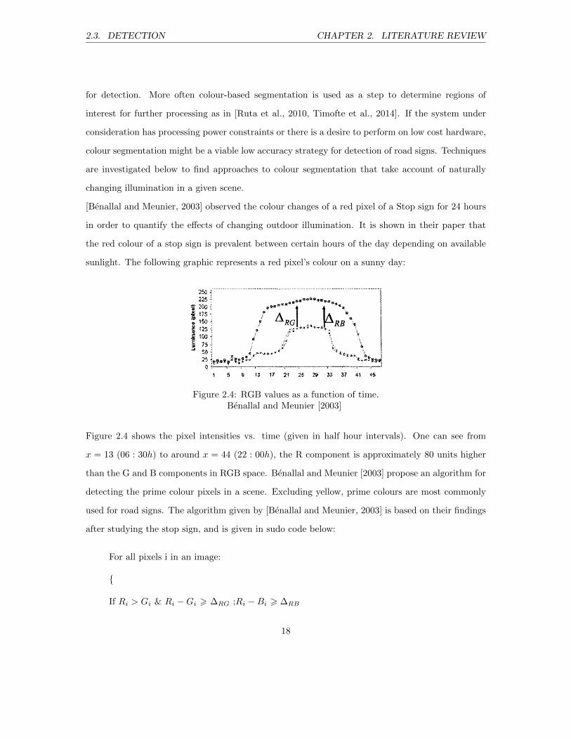
[Benallal and Meunier, 2003] observed the colour changes of a red pixel of a Stop sign for 24 hours
in order to quantify the effects of changing outdoor illumination. It is shown in their paper that
the red colour of a stop sign is prevalent between certain hours of the day depending on available
sunlight. The following graphic represents a red pixel’s colour on a sunny day:
Figure 2.4: RGB values as a function of time.Benallal and Meunier [2003]
Figure 2.4 shows the pixel intensities vs. time (given in half hour intervals). One can see from
x = 13 (06 : 30h) to around x = 44 (22 : 00h), the R component is approximately 80 units higher
than the G and B components in RGB space. Benallal and Meunier [2003] propose an algorithm for
detecting the prime colour pixels in a scene. Excluding yellow, prime colours are most commonly
used for road signs. The algorithm given by [Benallal and Meunier, 2003] is based on their findings
after studying the stop sign, and is given in sudo code below:
For all pixels i in an image:
{
If Ri > Gi & Ri −Gi > ∆RG ;Ri −Bi > ∆RB
18

2.3. DETECTION CHAPTER 2. LITERATURE REVIEW
Then pixel i is Red
Else If Gi > Ri & Gi −Ri > ∆GR ; Gi −Bi > ∆GB
Then pixel i is Green
Else If Bi > Gi & Bi −Gi > ∆BG ; Bi −Ri > ∆BR
Then pixel i is Blue
ELSE pixel i is (White or Black) EndIF
}
EndFor
[Estevez and Kehtarnavaz, 1996] choose to recognise red warning signs such as stop, yield and no-
entry signs. The approach is split into six modules: colour segmentation, RGB differencing, edge
detection, edge localisation, histogram extraction and classification. The first step is colour segmen-
tation and is considered to be the most important step in the chain [Estevez and Kehtarnavaz, 1996].
The paper was written in 1996 and due to processing constraints, a method for fast segmentation was
needed. Estevez and Kehtarnavaz [1996] determined a minimum recognisable resolution (MRR) of
4 pixels, which allowed fast segmentation and also ensured sign edges were not skipped during edge
detection. The MRR is effectively the distance, measured in pixels, between pixels that are to be pro-
cessed.
In order to handle changing light conditions, Estevez and Kehtarnavaz [1996] captured average
intensities from the top of the image(the region corresponding to the sky). These average values
were then used to set the RGB transformation parameters from the source image [Estevez and
Kehtarnavaz, 1996]. In this way, detection parameters can be more specific in given conditions,
resulting in fewer false positives. Applying specific parameters in changing scenes can be thought
of as better fitting the model to data.
Kastner et al. [2010] used the RGBY space (Red,Green,Blue and Yellow) which is thought to closely
model how a human eye works. Features such as DoG (Difference of Gaussians) and Gabor filter
kernels were weighted and used to generate an attention map where areas with higher values indicate
19

2.3. DETECTION CHAPTER 2. LITERATURE REVIEW
possible signs. These regions of interest were then passed onto the classification step. Details can
be found in Kastner et al. [2010].
2.3.2 Locate Potential ROI
In order to localise signs in an image, the contours around objects in the image need to be found. In
order to find the contours around objects, it is useful to first determine the edges of the object, and
find the closed contours around those edges. Edge detection is commonly used for operation on a
single channel image. Edges in images are locations where the brightness of pixels changes at a high
rate, therefore 1st and 2nd derivatives are often used in edge detection. Each pixel in an image, like
a function in 3 dimensions, has a rate of change (gradient) in all directions and a specific direction
in which this rate of change is a maximum. Gradient Magnitude images are a visual display of
the magnitude of brightness changes in a specific direction [Dawson-Howe, 2014]. First derivatives
have local maximums at edges while 2nd derivatives are zero at edges (where the sign of the value
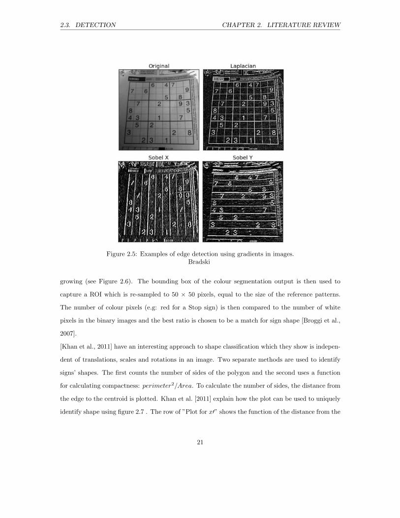
of the function changes)[Dawson-Howe, 2014]. In figure 2.5, one can see the outputs from different
image gradient types performed on the original image. ”Sobel X” finds edges in the horizontal (x)
direction while ”Sobel Y” finds gradients in the vertical direction. Laplacian finds a combination
of x and y gradients. Once the edges have been found, the contours can be determined. Closed
contours that have bounding rectangles with an aspect ratio close to 1 might contain signs. To
narrow down the potential regions of interest after performing this step, the area corresponding to
the average size of a sign in a frame may also be used as a filter.
2.3.3 Shape Determination
It is common to determine the shape of the sign before passing the region of interest onto classi-
fication[Khan et al., 2011]. This problem of determining the shape has been approached in many
different ways, some will be explored below. The process of determining shape is often referred to
as shape classification, which must not be confused with sign classification.
[Broggi et al., 2007] use pattern matching to detect the shapes of the colour segmented regions of
interest. They build a binary reference image for each shape that needs to be detected using region
20
2.3. DETECTION CHAPTER 2. LITERATURE REVIEW
Figure 2.5: Examples of edge detection using gradients in images.Bradski
growing (see Figure 2.6). The bounding box of the colour segmentation output is then used to
capture a ROI which is re-sampled to 50 × 50 pixels, equal to the size of the reference patterns.
The number of colour pixels (e.g: red for a Stop sign) is then compared to the number of white
pixels in the binary images and the best ratio is chosen to be a match for sign shape [Broggi et al.,
2007].
[Khan et al., 2011] have an interesting approach to shape classification which they show is indepen-
dent of translations, scales and rotations in an image. Two separate methods are used to identify
signs’ shapes. The first counts the number of sides of the polygon and the second uses a function
for calculating compactness: perimeter2/Area. To calculate the number of sides, the distance from
the edge to the centroid is plotted. Khan et al. [2011] explain how the plot can be used to uniquely
identify shape using figure 2.7 . The row of ”Plot for x′” shows the function of the distance from the
21

2.3. DETECTION CHAPTER 2. LITERATURE REVIEW
Figure 2.6: Binary Images used for Pattern MatchingBroggi et al. [2007]
Figure 2.7: Traffic Sign Shape Identification TechniqueKhan et al. [2011]
centroid to the edge as the x′ line rotates through 360◦ around the shape. Each parabola minimum
identifies another edge unlike the case of a circle which is represented by a straight line. Unique
values for perimeter2/Area as reported by Khan et al. [2011] can be seen in table 2.1.
If a sign passes the first test but fails the second, it is left to the sign classification that follows to
discard or identify the sign. The classification is achieved using Fringe-Adjusted Joint Transmission
Correlation (FJTC), details of which can be found in [Khan et al., 2011].
Lafuente-Arroyo et al. [2010] segment using the HIS colour space and channel thresholding, then
use the distance from an objects edge to a rectangular box that surrounds it (DtB) to determine
shape [Møgelmose et al., 2012]. A sign that is rectangular for example should have a distance
of zero for all sides while a triangular sign pointing downwards would have zero for the top only
22

2.3. DETECTION CHAPTER 2. LITERATURE REVIEW
Value Shape
9-11.75 Octagon11.8-14 Circle14.1-15.77 Pentagon15.78-19.14 Rectangle19.15-23 Triangle
Table 2.1: Values for perimeter2/Area function relation to shape
and the distances to the sides would increase as one moved down the sign. Once shape has been
determined using DtB, a region of interest is extracted from the source image and passed to the
specific shapes SVM. Separate SVMs were trained, with a Gaussian kernel, for each colour and
shape of sign [Lafuente-Arroyo et al., 2010].
2.3.4 Hybrid Approaches
[Ruta et al., 2011] proposed a quad-tree attention operator. The input image is initially filtered to
amplify red and blue using the formulas:
fR(x) = max
(0,min
(xR − xG
s,xR − xB
s
))fB(x) = max
(0,min
(xB − xR
s,xB − xG
s
)) (2.3)
xR, xB , and xG in equation 2.3 represent the red, blue and green components of pixel respectively
and s = xR + xB + xG [Ruta et al., 2011]. The output is an image representing red and another
representing blue. Ruta et al. [2011] then compute a gradient magnitude map (2.3.2) of each image
(fR(x) and fB(x)) passing the output to find the integral images for each colour. If either integral
image has values higher than a chosen threshold, the image is split into four regions and the process
is repeated for each region. This happens recursively until no maximums are above the threshold,
or the minimum region size is reached. Thereafter adjacent clusters are combined if they meet the
gradient requirements forming regions of interest to be passed onto the sign detection step [Ruta
et al., 2011].
Viola [2001] made a significant contribution to the field of object detection. Their method which
23

2.4. CLASSIFICATION CHAPTER 2. LITERATURE REVIEW
is often used for facial recognition, is capable of processing images very quickly while maintaining
high recognition rates. They proposed the ”Integral Image” and use a learning algorithm based on
AdaBoost which use a combination of weak features to create a strong classifier. The detector is
trained using a large collection of positive and negative images. Positive images contain the object
to be detected, and negative images are background images that contain features to be ignored by
the algorithm.
2.4 Classification
Classification of traffic signs is a difficult problem due to the high sub-class variability and object
variations caused by changes in position of viewpoint over time. The large natural variations in
illumination and contrast make the task even more challenging. The human brain and vision
system can easily differentiate between signs. It is no wonder then that some of the most accurate
classification techniques use architectures that mimic the nature of the human visual cortex. Popular
approaches to classification are explored in this section.
2.4.1 Support Vector Machines (SVM)
Figure 2.8: SVM hyperplane in 2 dimensionsBradski
24

2.4. CLASSIFICATION CHAPTER 2. LITERATURE REVIEW
SVMs [Cristianini and Shawe-Taylor, 2000] attempt to find the optimal hyper-plane for use in
separating multidimensional classes and thus facilitating feature vector classification (see figure
2.8). The hyper-plane, as shown in Figure 2.8, is found such that it is a maximum distance from
the support vectors. The support vectors are the feature vectors used for training that belong
to separate classes and are closest to the classification boundary (the solid shapes in Figure 2.8).
Boi and Gagliardini [2011] perform TSR in two stages, a pre-processing stage and a classification
stage. The preprocessing stage extracts features using Hue Histogram and a Histogram of Oriented
Gradients (HoG) [Boi and Gagliardini, 2011] . The classification is accomplished using a sequence
of SVMs that are implemented with a One Versus All methodology. The One vs All approach is
used in machine learning for multi-class classifications and involves training a classifier for each class
where each classes samples are either positive or negative [Bishop, 2006]. The classifier also returns
a value of confidence so that no ambiguity exists when many classes are predicted for individual
features [Boi and Gagliardini, 2011, Bishop, 2006].
Using a Gaussian Kernal in the SVM provides better results than linear and polynomial kernels [Boi
and Gagliardini, 2011] and all SVMs used by Boi and Gagliardini [2011] have a Gaussian kernel.
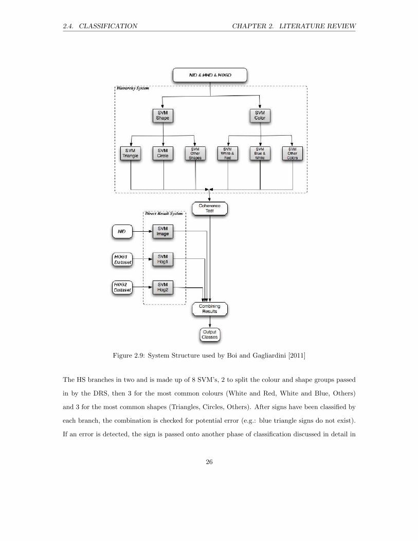
Their entire network is split into two main modules (see figure 2.9); Hierarchical System (HS) and
Direct Result System (DRS). The DRS determines the sign’s class by colour and shape using three
separate SVMs, each with a measure of reliability [Boi and Gagliardini, 2011].
25
2.4. CLASSIFICATION CHAPTER 2. LITERATURE REVIEW
Figure 2.9: System Structure used by Boi and Gagliardini [2011]
The HS branches in two and is made up of 8 SVM’s, 2 to split the colour and shape groups passed
in by the DRS, then 3 for the most common colours (White and Red, White and Blue, Others)
and 3 for the most common shapes (Triangles, Circles, Others). After signs have been classified by
each branch, the combination is checked for potential error (e.g.: blue triangle signs do not exist).
If an error is detected, the sign is passed onto another phase of classification discussed in detail in
26

2.4. CLASSIFICATION CHAPTER 2. LITERATURE REVIEW
Boi and Gagliardini [2011].
2.4.2 Convolutional Neural Networks (CNN)
Among the most accurate methods of classification are those that use convolution neural networks
[Jarrett et al., 2009, Ciresan et al., 2012]. CNNs are inspired by biological processors (organic
brains) and are composed of multi-level architectures that automatically learn hierarchies of invari-
ant features through a combination of unsupervised and supervised learning techniques [Sermanet
and LeCun, 2011]. Popular for their low requirements for pre-processing and for being robust to
distortions [LeCun et al., 2010].
Architecture
De La Escalera et al. [1997] achieved detection through colour thresholding and other heuristic
methods that returned sub-regions with a specification on shape. Different Multi-Layer NNs were
then used to recognise subclasses for each shape. The De La Escalera et al. [1997] NNs consist of 3
layers with at most 30, 15 and 10 hidden units for each taking an input image with 30×30 pixels.
Sermanet and LeCun [2011] modified the common CNN architecture by feeding additional 2nd stage
features into the classifier. The goal was to build a robust recognition system without the need for
temporal information. Sermanet and LeCun [2011] suggest that is it becoming more commonplace
to divide detection and recognition(classification) into separate steps, choosing to spend resources on
the classification step and choose less computationally expensive methods for detection such as color
thresholding. The paper had recognised that the most common approaches for TSR classification
include Support Vector Machines (SVM) and Neural Networks (NN). Sermanet and LeCun [2011]
addressed TRS as a general vision problem, and as such did not need to make assumptions on sign
colours or shapes that would result in low recognition rates if the system were tested on different
international datasets. Their approach to recognition was to use Convolution Neural Networks
with a convolution, a non-linear transform and a spatial feature pooling layer Sermanet and LeCun
[2011]. The pooling layers lower the resolution of the image, this is understood to remove the effects
of minor shifts and geometric distortions. The usual approach with CNN is to pass only the final
27
2.4. CLASSIFICATION CHAPTER 2. LITERATURE REVIEW
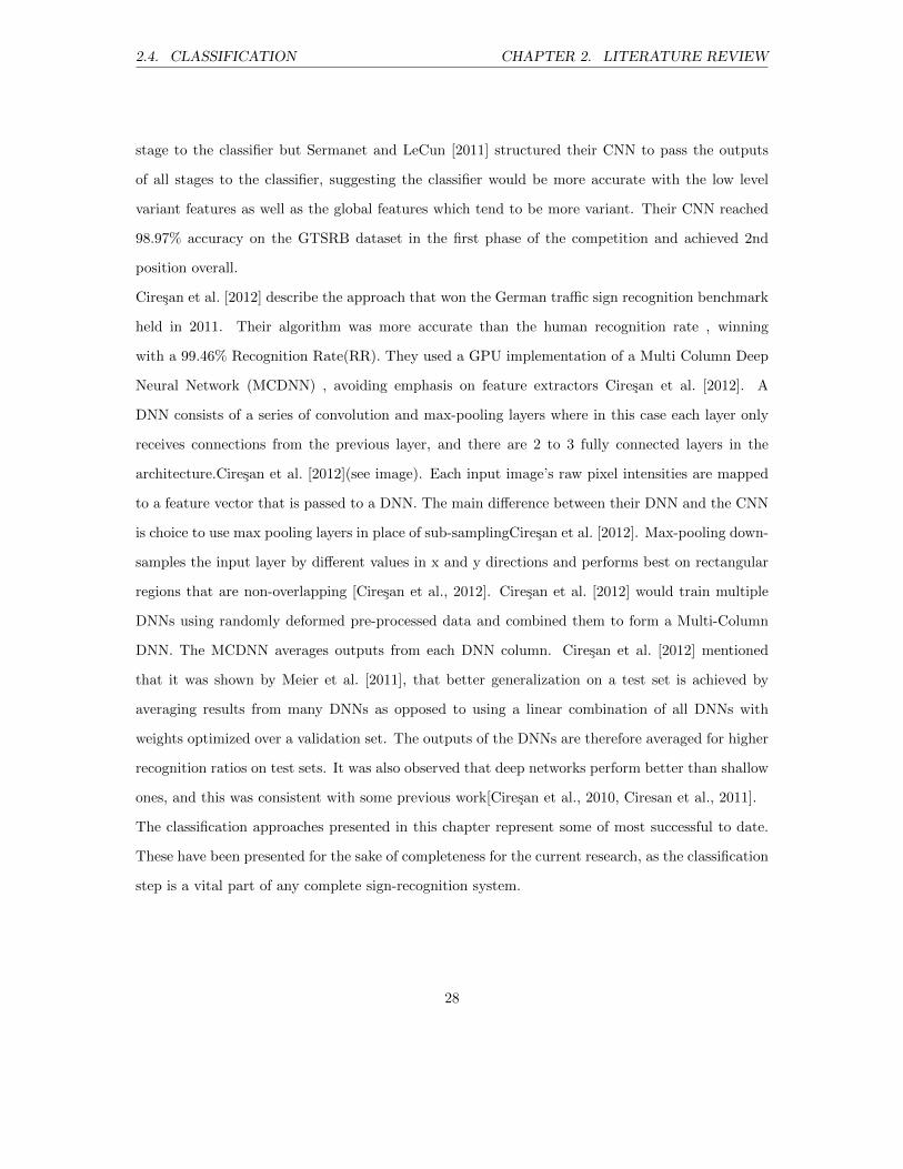
stage to the classifier but Sermanet and LeCun [2011] structured their CNN to pass the outputs
of all stages to the classifier, suggesting the classifier would be more accurate with the low level
variant features as well as the global features which tend to be more variant. Their CNN reached
98.97% accuracy on the GTSRB dataset in the first phase of the competition and achieved 2nd
position overall.
Ciresan et al. [2012] describe the approach that won the German traffic sign recognition benchmark
held in 2011. Their algorithm was more accurate than the human recognition rate , winning
with a 99.46% Recognition Rate(RR). They used a GPU implementation of a Multi Column Deep
Neural Network (MCDNN) , avoiding emphasis on feature extractors Ciresan et al. [2012]. A
DNN consists of a series of convolution and max-pooling layers where in this case each layer only
receives connections from the previous layer, and there are 2 to 3 fully connected layers in the
architecture.Ciresan et al. [2012](see image). Each input image’s raw pixel intensities are mapped
to a feature vector that is passed to a DNN. The main difference between their DNN and the CNN
is choice to use max pooling layers in place of sub-samplingCiresan et al. [2012]. Max-pooling down-
samples the input layer by different values in x and y directions and performs best on rectangular
regions that are non-overlapping [Ciresan et al., 2012]. Ciresan et al. [2012] would train multiple
DNNs using randomly deformed pre-processed data and combined them to form a Multi-Column
DNN. The MCDNN averages outputs from each DNN column. Ciresan et al. [2012] mentioned
that it was shown by Meier et al. [2011], that better generalization on a test set is achieved by
averaging results from many DNNs as opposed to using a linear combination of all DNNs with
weights optimized over a validation set. The outputs of the DNNs are therefore averaged for higher
recognition ratios on test sets. It was also observed that deep networks perform better than shallow
ones, and this was consistent with some previous work[Ciresan et al., 2010, Ciresan et al., 2011].
The classification approaches presented in this chapter represent some of most successful to date.
These have been presented for the sake of completeness for the current research, as the classification
step is a vital part of any complete sign-recognition system.
28

2.5. TRAINING AND TESTING CHAPTER 2. LITERATURE REVIEW
2.5 Training and Testing
2.5.1 Techniques for Robustness to Deformations in ROI
Sermanet and LeCun [2011] added random distortions to their training set, 5 additional images
of each sign with changes in rotation([-15,+15] degrees) ,position([-2,2] pixels) and scale([0.9,1.1]
ratio). This ensures the images contain deformations that might not occur naturally in dataset,
making the classification more robust to deformations during testing [Sermanet and LeCun, 2011].
Figure 2.10: Performance Difference between Training SetsBradski
Figure 2.10 shows the performance difference when tested on a subset of the GTSRB dataset. Other
effects to potentially improve the training set include different affine transformations, changes in
brightness, motion blur effects and contrast variations [Sermanet and LeCun, 2011].
Ciresan et al. [2012] used a Multi Column Deep Neural Network and distorted input images in
much the same way as Sermanet and LeCun [2011]. Rotation([-5,5] degrees), scaling([0.9,1.1] ratio)
and translation([0.9,1.1] ratio) where the final image with a set size is obtained using bilinear
interpolation. The error rate improvement in the GTSRB dataset (first phase) decreased from
2.83% to 1.66% [Ciresan et al., 2012]. Ciresan et al. [2012] randomized the weights of each column
before training and also normalized the input data differently for each column in the MCDNN.
Having highly correlated columns needs to be avoided and without the changes in normalisation of
the input data, the DNNs from different columns run this risk of correlation Ciresan et al. [2012].
This has shown the importance of variation during training. This variation ensures the classifier
will perform well on general datasets and will not over-fit to the dataset used for training.
2.5.2 Bootstrapping
Boi and Gagliardini [2011] uses a method called bootstrapping during their training and testing.
This allows a sampling operation using the original dataset, the GTSRB. Bootstrapping means
29

2.5. TRAINING AND TESTING CHAPTER 2. LITERATURE REVIEW
collecting samples at random to add to a training set and using the remaining pictures in the
original dataset to test the system. This is repeated n times. Random selection of pictures prevents
any deterministic structure from influencing the results and Boi and Gagliardini [2011] chose to
perform 10 repetitions to average the recognition rate.
This concludes the chapter on relevant methods in current literature. The following chapter will
present the proposed method, that intends to efficiently detect the locations of traffic signs in video,
while classifying shape. The output of the proposed system would feed into a sign-classifier in order
to complete the sign recognition system.
2.5.3 Summary
This lit review has highlighted some useful techniques to overcoming the most common challenges
in traffic sign detection. The methods that are most relevant are those that offered improved
performance without a loss in accuracy. The RGB thresholding approach using colour ranges would
be suitable for a high performance system because no transformation is needed for input frames,
and colour segmentation has been shown to be very efficient. The decision to skip unnecessary
pixels in high resolution video also offered significant performance improvements. Of the shape
determination methods, the binary image pattern matching approach may be best suited to a high
performance system; the method proposed by Khan et al. [2011] requires more computations to
make a shape classification. Support Vector Machines have been shown to be a popular approach
to classification, and may be of interest when determining shape during detection. The neural
networks, which were shown to be the most successful classification approaches, may benefit from
having regions of interest with extra information such as shape. This would serve to reduce the
number of possibilities for signs along a given tree as in Figure 2.9. The techniques covered in
this chapter inspired experimentation and the most promising were eventually implemented in the
proposed system. The proposed method will be covered in the following chapter.
30

Chapter 3
Method
3.1 Overview of Method
Two separate methods will be discussed. The first is the proposed method for performance in a
given lighting situation and will be covered first in this chapter. The second is the training approach
used for the creation of Cascade Classifiers which are used during the experiments. The Cascade
Classification method was first presented by Viola [2001].
3.1.1 Proposed System Design
From a broad perspective; individual frames are passed into the system from an input video as
shown in 3.1. The detection system then processes frames until a sign candidate is found with an
associated shape. This candidate is finally passes to an external sign classifier. The detection unit,
which is the proposed method, can be broken down further. This method will be presented in the
same order as the flow of data through the sign detector as shown in the figure 3.1.
The preprocessing and segmentation will be covered first. Then classification stage in this approach
is split into two subgroups which could operate independently but together add redundancy; SVM
classification and Binary Image Testing. These then converge into the sub-section which deals with
tracking of the signs in images, and finally the decision on shape and region which would be passed
31

3.1. OVERVIEW OF METHOD CHAPTER 3. METHOD
to a sign classifier.
Figure 3.1: Overview of the Proposed Method
32
3.1. OVERVIEW OF METHOD CHAPTER 3. METHOD
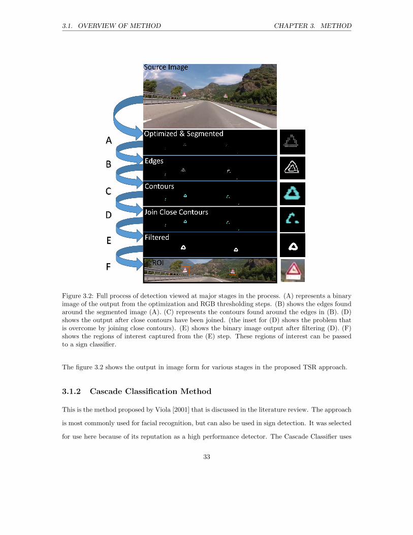
Figure 3.2: Full process of detection viewed at major stages in the process. (A) represents a binaryimage of the output from the optimization and RGB thresholding steps. (B) shows the edges foundaround the segmented image (A). (C) represents the contours found around the edges in (B). (D)shows the output after close contours have been joined. (the inset for (D) shows the problem thatis overcome by joining close contours). (E) shows the binary image output after filtering (D). (F)shows the regions of interest captured from the (E) step. These regions of interest can be passedto a sign classifier.
The figure 3.2 shows the output in image form for various stages in the proposed TSR approach.
3.1.2 Cascade Classification Method
This is the method proposed by Viola [2001] that is discussed in the literature review. The approach
is most commonly used for facial recognition, but can also be used in sign detection. It was selected
for use here because of its reputation as a high performance detector. The Cascade Classifier uses
33
3.2. PREPROCESSING CHAPTER 3. METHOD
a combination of weak features found in the integral images of input frames to make classifications.
The approach to training the Cascade Classifier will be covered after the proposed method has been
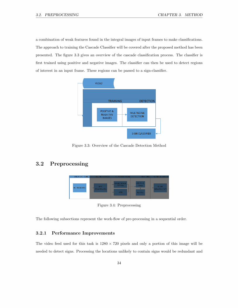
presented. The figure 3.3 gives an overview of the cascade classification process. The classifier is
first trained using positive and negative images. The classifier can then be used to detect regions
of interest in an input frame. These regions can be passed to a sign-classifier.
Figure 3.3: Overview of the Cascade Detection Method
3.2 Preprocessing
Figure 3.4: Preprocessing
The following subsections represent the work-flow of pre-processing in a sequential order.
3.2.1 Performance Improvements
The video feed used for this task is 1280 × 720 pixels and only a portion of this image will be
needed to detect signs. Processing the locations unlikely to contain signs would be redundant and
34
3.2. PREPROCESSING CHAPTER 3. METHOD
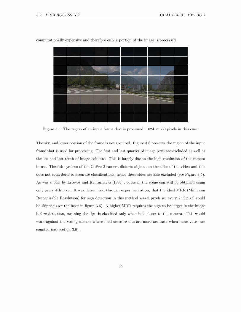
computationally expensive and therefore only a portion of the image is processed.
Figure 3.5: The region of an input frame that is processed. 1024 × 360 pixels in this case.
The sky, and lower portion of the frame is not required. Figure 3.5 presents the region of the input
frame that is used for processing. The first and last quarter of image rows are excluded as well as
the 1st and last tenth of image columns. This is largely due to the high resolution of the camera
in use. The fish eye lens of the GoPro 2 camera distorts objects on the sides of the video and this
does not contribute to accurate classifications, hence these sides are also excluded (see Figure 3.5).
As was shown by Estevez and Kehtarnavaz [1996] , edges in the scene can still be obtained using
only every 4th pixel. It was determined through experimentation, that the ideal MRR (Minimum
Recognisable Resolution) for sign detection in this method was 2 pixels ie: every 2nd pixel could
be skipped (see the inset in figure 3.6). A higher MRR requires the sign to be larger in the image
before detection, meaning the sign is classified only when it is closer to the camera. This would
work against the voting scheme where final score results are more accurate when more votes are
counted (see section 3.6).
35
3.3. SEGMENTATION CHAPTER 3. METHOD
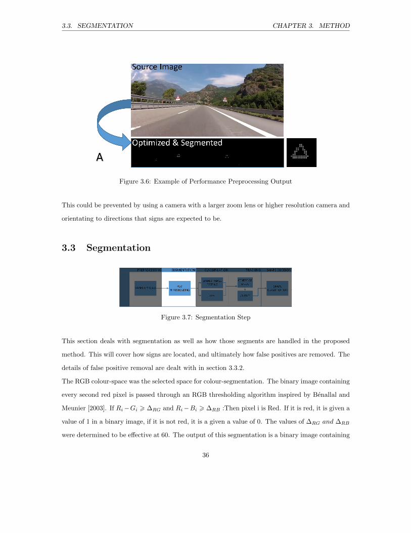
Figure 3.6: Example of Performance Preprocessing Output
This could be prevented by using a camera with a larger zoom lens or higher resolution camera and
orientating to directions that signs are expected to be.
3.3 Segmentation
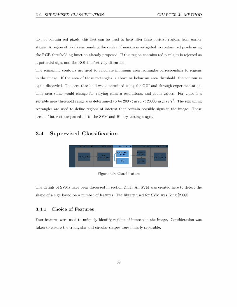
Figure 3.7: Segmentation Step
This section deals with segmentation as well as how those segments are handled in the proposed
method. This will cover how signs are located, and ultimately how false positives are removed. The
details of false positive removal are dealt with in section 3.3.2.
The RGB colour-space was the selected space for colour-segmentation. The binary image containing
every second red pixel is passed through an RGB thresholding algorithm inspired by Benallal and
Meunier [2003]. If Ri−Gi > ∆RG and Ri−Bi > ∆RB :Then pixel i is Red. If it is red, it is given a
value of 1 in a binary image, if it is not red, it is a given a value of 0. The values of ∆RG and ∆RB
were determined to be effective at 60. The output of this segmentation is a binary image containing
36

3.3. SEGMENTATION CHAPTER 3. METHOD
dense clusters of white pixels that represent regions of interest.
Figure 3.8: A visual overview of the steps in the detection of ROI.
Figure 3.8 follows from the example in figure 3.6. It extends the example showing outputs in the
various stages of detection. The sections to follow are structured in the same sequential manner as
represented in figure 3.8.
The input image/frame here is in binary format where white pixels signify potential signs’ red pixel
locations. There is expected to be a lot of noise from buildings, other vehicles and other red objects
in the scene, as noise removal was not implemented in the preprocessing stage. These pixels do not
represent signs and need to be removed now in order to reduce false positive detections.
3.3.1 Locate Signs
Contours are detected around groups of white pixels in the binary image. The output of this stage
is passed on to an edge detection step. An example of an output of these stages can be seen in
37

3.3. SEGMENTATION CHAPTER 3. METHOD
Figure 3.8. The stage still contains noise from objects other than signs, these effects are mitigated
in the steps that follow.
3.3.2 Filter Noise
Noise removal is often performed after the preprocessing step in common detection systems. In this
approach, noise is handled after regions of interest have been found.
Combine Close Contours
After the vector of contours is found for all edges, the centre of mass is calculated for each contour.
There are often cases where there will be multiple contours around a single sign. This may be due
to poor sign conditions, or when the sign in still far from the camera. In such cases, in order to
obtain a region of interest around the entire sign and not just sections of it, close contours must be
joined to form single areas.
Space Partitioning
In order to accomplish the close contour combinations, the centre points need to have point prox-
imity awareness . A useful data structure in such a scenario is the k-dimensional tree (k-d tree).
This structure partitions k dimensional space and organises points contained within the partitions.
This makes it useful for quick nearest neighbour analysis within multidimensional data.
A 2D k-d tree was created and used to store the Centres Of Mass. Then a nearest neighbours search
was used to find points within a definable region (this region can be set using the GUI) for every
point representing a mass centre. Groups of points in common areas within the regions are then
joined by lines, ensuring the contours around the regions connect. Contours are recalculated based
on the updated areas, and their centres of mass are recalculated and passed onto the next step.
False Positives Removal
False positives are removed at this stage using the colour at the centre of the ROI and the area and
aspect ration of the ROI. These are discussed in more detail below. The centre of signs to classify
38
3.4. SUPERVISED CLASSIFICATION CHAPTER 3. METHOD
do not contain red pixels, this fact can be used to help filter false positive regions from earlier
stages. A region of pixels surrounding the centre of mass is investigated to contain red pixels using
the RGB thresholding function already proposed. If this region contains red pixels, it is rejected as
a potential sign, and the ROI is effectively discarded.
The remaining contours are used to calculate minimum area rectangles corresponding to regions
in the image. If the area of these rectangles is above or below an area threshold, the contour is
again discarded. The area threshold was determined using the GUI and through experimentation.
This area value would change for varying camera resolutions, and zoom values. For video 1 a
suitable area threshold range was determined to be 200 < area < 20000 in pixels2. The remaining
rectangles are used to define regions of interest that contain possible signs in the image. These
areas of interest are passed on to the SVM and Binary testing stages.
3.4 Supervised Classification
Figure 3.9: Classification
The details of SVMs have been discussed in section 2.4.1. An SVM was created here to detect the
shape of a sign based on a number of features. The library used for SVM was King [2009].
3.4.1 Choice of Features
Four features were used to uniquely identify regions of interest in the image. Consideration was
taken to ensure the triangular and circular shapes were linearly separable.
39
3.4. SUPERVISED CLASSIFICATION CHAPTER 3. METHOD
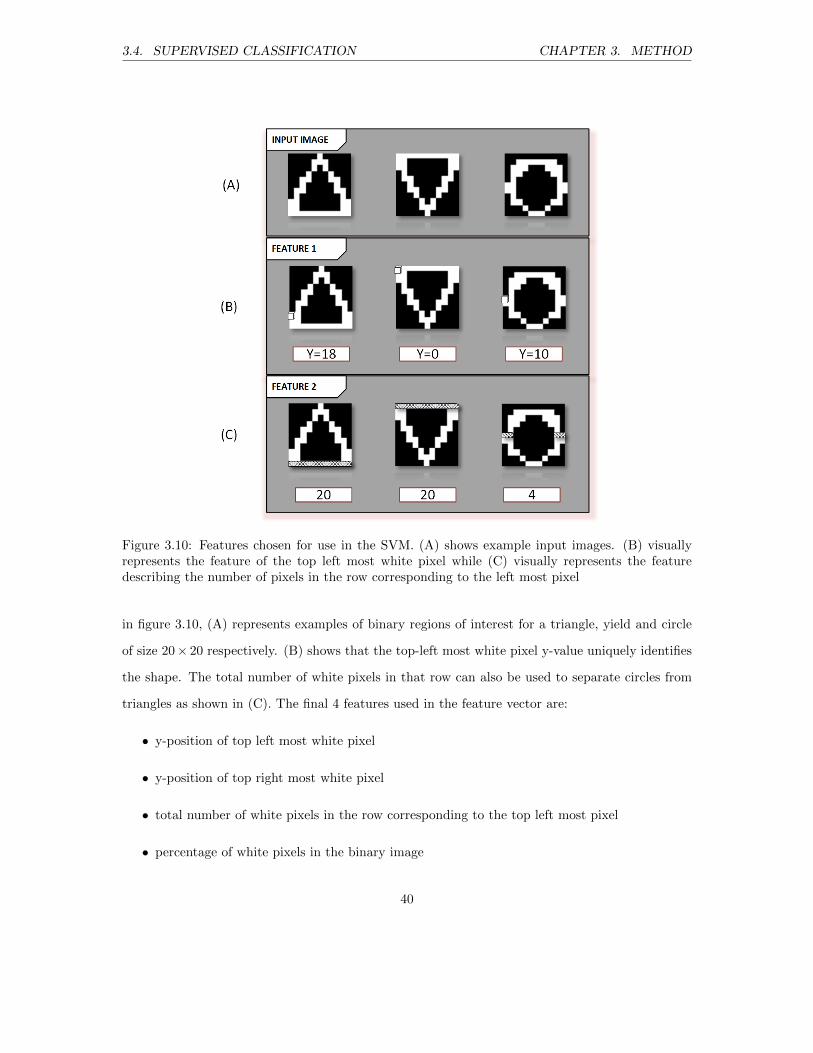
Figure 3.10: Features chosen for use in the SVM. (A) shows example input images. (B) visuallyrepresents the feature of the top left most white pixel while (C) visually represents the featuredescribing the number of pixels in the row corresponding to the left most pixel
in figure 3.10, (A) represents examples of binary regions of interest for a triangle, yield and circle
of size 20× 20 respectively. (B) shows that the top-left most white pixel y-value uniquely identifies
the shape. The total number of white pixels in that row can also be used to separate circles from
triangles as shown in (C). The final 4 features used in the feature vector are:
• y-position of top left most white pixel
• y-position of top right most white pixel
• total number of white pixels in the row corresponding to the top left most pixel
• percentage of white pixels in the binary image
40

3.5. BINARY IMAGE TEMPLATE MATCHING CHAPTER 3. METHOD
The last feature in the list is also used to filter out noise. Regions of interest containing only noise
often have a white to black ratio of over 50% in the binary image (these would be red pixels in the
colour region of interest).
3.4.2 Training
In order to train the SVM, the detection program was executed and detected regions of interest
were saved to disk. These regions were then separated into the 3 classes; circle, triangle and yield.
These classes are used as labels for the images when the SVM is trained. The SVM training script
saves a .dat file which can then be loaded into a classifier and used to classify an unknown feature
vector.
3.4.3 Classify Shape
The .dat file was loaded into the scope of the TSR program and is used to classify a feature vector
that is created for every region of interest. The feature vector in the TSR program has the same
order of features as the vector used for training. The classification returns a key which is associated
with a label. This label is then associated with the region of interest. Before the labelled region
of interest is passed onto a tracking stage, it can be compared to the output of the binary image
testing step. If the labels are the same, it will be passed onto the tracking stage. If the labels differ,
one of the shape classifiers was incorrect or the ROI contains noise only. In both cases the ROI is
discarded until the next frame is passed to the detector.
3.5 Binary Image Template Matching
The detection of shape can be accomplished using binary image addition with a template as shown
in figure 3.11.
The figure shows an input image, the shape templates and the result of the binary addition. White
plus white will return white, all other combinations return black. The total white number of pixels
is counted and the associated shape is given a vote.
41

3.5. BINARY IMAGE TEMPLATE MATCHING CHAPTER 3. METHOD
Figure 3.11: Example for Binary Addition Arithmetic shape classification. The input image issummed with a template. The resulting image pixels are counted and a vote is cast for shape.
The input image will not always be a perfect shape due to natural variations in the signs rotation,
wear and tear on the signs and illumination conditions. Also, partial occlusions may affect the
binary image input.It is therefore necessary to use a voting scheme over a number of frames.
On average, the shape of sign will be represented in the result of the addition. It is therefore
required to keep track of signs position in the image, and keep a tally of the results returned. A
mean may then be calculated to determine the likeliest shape at a position in the image. This
tracking stage will be discussed in the next section.
42
3.6. CANDIDATE SIGN TRACKING CHAPTER 3. METHOD
3.5.1 Checks
There is another opportunity to filter out noise and avoid false positives. Two more binary images
are used to accomplish this. A common characteristic between all signs is that they are symmetric
from the front, when no tilt is present. Therefore it can be expected that there will be no blank
halves in the input image. A white left half binary and a white right half binary image is used to
test for these cases. The image addition is applied to and input image and if the output image has
fewer than 4 pixels, the region of interest can be discarded. The last check is based on the fact
that the sum of total pixels from the triangle result and circle result must be higher than a given
value. This is used to discard regions of interest with too few white pixels to use for a reliable vote
on shape.
3.6 Candidate Sign Tracking
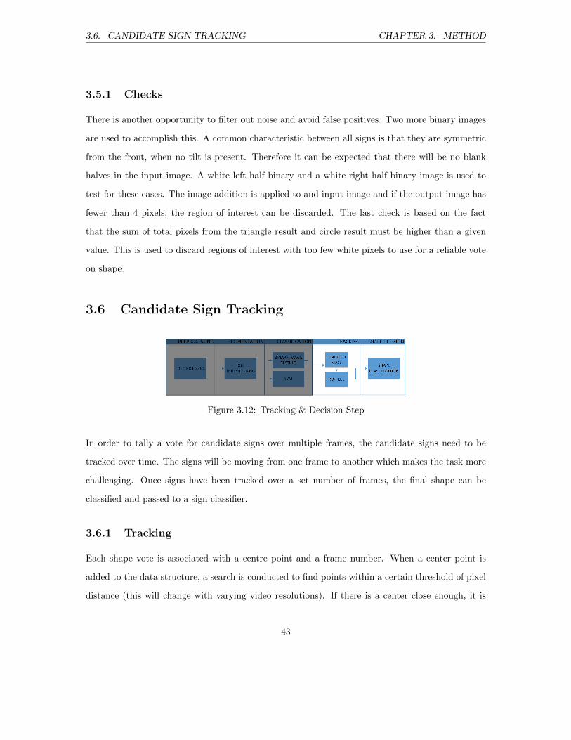
Figure 3.12: Tracking & Decision Step
In order to tally a vote for candidate signs over multiple frames, the candidate signs need to be
tracked over time. The signs will be moving from one frame to another which makes the task more
challenging. Once signs have been tracked over a set number of frames, the final shape can be
classified and passed to a sign classifier.
3.6.1 Tracking
Each shape vote is associated with a centre point and a frame number. When a center point is
added to the data structure, a search is conducted to find points within a certain threshold of pixel
distance (this will change with varying video resolutions). If there is a center close enough, it is
43

3.7. CASCADE CLASSIFIER DETECTION CHAPTER 3. METHOD
assumed to be the same sign, and the vote is added to the current tally. If there is no existing
center within the distance threshold, a new member is created to represent the new region.
Once a shape has been tracked for a given number of consecutive frames and has a vote for shape,
the classification of shape and its associated region of interest can be passed onto a sign classifier.
This region of interest should be largely free from false positives. A successful approach to sign
classification is the Convolutional Neural Network, discussed in detail in section 2.4.2.
3.6.2 Deleting Old ROIs and Final Sign Shape Classification
With every frame, centres are deleted if they have not moved for over 7 frames. This value will
need adjustment for frame rates substantially lower or higher than 25 fps. As signs move out of the
field of view of the camera, their voting scheme system can be discarded. However, there must be a
sufficient number of passing frames before this decision is made. This is to ensure voting scheme for
centres are not deleted for temporary occlusions. For over 7 frames, the distance between successive
centres of an occluded candidate will be over the threshold, and a new voting scheme structure will
be created for the new position.
3.7 Cascade Classifier Detection
Viola [2001] made a big contribution to facial recognition, and this paper has also inspired use in
traffic sign recognition. OpenCV [Bradski] have extended the Viola [2001] algorithm with Lienhart
et al. [2003] and also allow for use of LBP (local binary pattern) features in addition to Haar-like
features.
3.7.1 Training
A separate directory is created for positive and negative images. Positive images contain the feature
to detect, and negative images are background images that do not contain the feature. It is necessary
to build a collection of background images that can be used for training. During the early stages
of training, the GTSRB [GTS, 2012] images were used as positive images. Random background
44

3.7. CASCADE CLASSIFIER DETECTION CHAPTER 3. METHOD
images were collected and used for the training. Once the classifier was trained, it was saved to disk.
Using the TSR program, the .xml was loaded and run to detect possible sign. All detected regions
were saved to disk. False positives were then used as background images and the cascade classifier
was retrained. This process was repeated until the detection was accurate and false positives were
minimised.
3.7.2 Detection
A separate classifier was trained for circular signs, triangular signs and stop signs. Another classifier
was trained containing all three types. The program was run using the detection for all signs and
the performance (time in m seconds) was recorded. The program was then run using the three
separate classifiers and the performance was recorded. It was to be expected that the combined
classifier would outperform multiple classifiers, however using multiple classifiers gives feedback
on the detected shape, which can be used to improve classification efficiency and in some cases
accuracy.
45

Chapter 4
Results
4.1 Testing Methodology
Two detection methods will be compared; Cascade Classification and the proposed method. The
popular approach of using a Cascade Classifier for detection was implemented in two ways. The
first being a group of separate classifiers for circular shapes, yield sign (upside down triangle) and
triangular signs. This approaches gives feedback on the shape of the sign as well as detecting its
position in the image. The second cascade detection approach was trained using all possible sign
shapes. This means the detector was able to detect regions that contain signs but could not give
feedback on the shape of the sign.
The proposed detection contains two main components that are used to detect shape. The SVM and
the binary image classifier (see figure 3.1). The shape classification accuracy of each was measured
independently. Thereafter, another test was conducted with the full proposed design, where both
components were used for redundancy and improved reliability.
To evaluate the detection methods, 2 video sequences totalling 7900 frames, containing 3 groups
of signs were used. Video was captured in daylight scenes with the camera mounted on the front
of a motor vehicle in a low elevation. Video 1 was broken into 11 clips to facilitate comparison in
different conditions (see Figure: 4.1). Video 2 represents challenging detection situations where low
46
4.1. TESTING METHODOLOGY CHAPTER 4. RESULTS
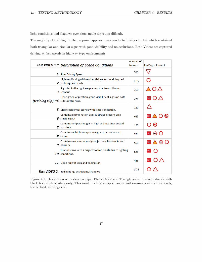
light conditions and shadows over signs made detection difficult.
The majority of training for the proposed approach was conducted using clip 1.4, which contained
both triangular and circular signs with good visibility and no occlusions. Both Videos are captured
driving at fast speeds in highway type environments.
Figure 4.1: Description of Test-video clips. Blank Circle and Triangle signs represent shapes withblack text in the centres only. This would include all speed signs, and warning sign such as bends,traffic light warnings etc.
47

4.1. TESTING METHODOLOGY CHAPTER 4. RESULTS
4.1.1 Reliability of the Detector
The detection rate refers to the percentage of true detections to total number of signs. The higher
the detection rate, the more reliable the detector is to pass regions of interest onto the sign classifier.
The following detection rates were determined:
• the detection rate of the proposed system
• the detection rate of the combined cascade classifier
• the detection rate using multiple sign cascade classifiers
4.1.2 Shape Classification
This is not a requirement for a sign detector, but shape classification does contribute to make the
signs classification more efficient. It accomplishes this by limiting the number of possibilities in
a given classification tree (refer to section 2.4.2). The shape classification refers to the process of
determining the shape of a sign in a detected region. The shape recognition rate is the percentage
of correct classifications to total shapes input into the classifier. Once the shape was classified in
each approach from the test videos, a supervisor determined if the shape was correct or incorrect.
False shape classifications were also recorded (classification of shape in a region not containing a
sign). The following is an overview of what tests were conducted:
• shape recognition rate of the SVM
• shape recognition rate of the Binary Image Arithmetic approach
• shape recognition rate of the combination between the SVM and the Binary Image Arithmetic
approaches
• shape recognition rate using multiple sign cascades
All results are shown in the following section in summarised, tabulated form.
48

4.2. EXPERIMENT RESULTS CHAPTER 4. RESULTS
4.2 Experiment Results
Figure 4.2: Overview of the Proposed Method
This chapter will briefly discuss the expected outcomes and observations made in each sub-section
seen in Figure 4.2. The decisions made during development were based on results obtained during
the training. The chapter goes on to present the results from the testing approach defined in section
(4.1).
4.2.1 Components of the proposed system
The proposed system was developed on Debian Linux using C++, QT framework and OpenCV
2.4.11. The method is best suited to the GoPro 2 camera, in daylight conditions.
Preprocessing
The preprocessing of input frames for the camera was limited to reducing the region of interest in the
original frame and processing only every second pixel. In the cases where Cascade Classifiers were
used for detection, every third frame was processed but without skipping pixels. This was due to the
performance constraints of the cascade methods as shown in Table 4.5. The proposed method was
able to process every frame in the 25 fps input video without skipping every second pixel, however
this made no significant improvement to detection. Thus the skipping pixel implementation was
used for performance benefits. Common preprocessing techniques such as contrast stretching and
Gaussian blur were explored, but made no improvement to detection in the proposed method. This
was due to the manner in which contours were filtered later in the approach. Using mass centre and
49

4.2. EXPERIMENT RESULTS CHAPTER 4. RESULTS
minimum bounding rectangle area constraints to remove noise proved more effective than applying
these common preprocessing techniques. This meant implementing filters in the early stages would
not help detection and only reduce performance. These common preprocessing steps are thus not
required in the proposed method.
Segmentation
It has been shown that the most common approach to segmentation in an input frame is to use
some form of colour-space thresholding. The most common colour space used in visual applications
is HSV.
This is due to the direct access to hue, which is easier for human interpretation and manipulation.
Binary output images from both colour spaces were compared in the proposed approach and it was
shown that the RGB technique was more successful at segmenting red signs (see Figure 4.3). The
chosen RGB segmentation approach is covered in section 3.3. The HSV thresholds in the figure
4.3 were set to the following generous ranges: Hue: 134-180, Saturation : 0-155, Value 0-255 in
OpenCV’s ”inRange” method. The segmented output image does not contain all signs even with
the generous red hue ranges. Also, the HSV segmentation contains more noise (non-signs). This
led to the conclusion that the RGB thresholding ranges led to better segmentation for input frames
using the GoPro 2 camera the Test Video 1 lighting conditions, and was the segmentation method
of choice in the proposed approach.
50

4.2. EXPERIMENT RESULTS CHAPTER 4. RESULTS
Figure 4.3: Comparison between RGB and HSV thresholding. In (B) , output pixels are black when(R−B) > 60 and (R−G) > 60. In (C), HSV values were set to threshold all Hue values between134-180. (openCV uses a hue range between 0 and 180 as opposed to the common range of 0-360)High levels of noise can be seen in (C). The black pixels in (C) are the pixels segmented using HSVthresholding.
Classification
In order to compare the results of shape classification for this detection system, 3 tests were set-up.
The first test used only the SVM described in section 2.4.1 to classify the shape. The second used
only the binary shape arithmetic described in section 3.5 and the third used a combination of both.
The combination approach only assigns a label in the case both classifiers agree on shape. The tests
were run on all 11 clips from Video 1 and the tabulated results are shown below in table 4.1.
Table 4.1 shows that the SVM classifier obtained the most true positives, however, the SVM also
51

4.2. EXPERIMENT RESULTS CHAPTER 4. RESULTS
Table 4.1: Tabulated results from TSR using only the SVM for shape classification. True posi-tives(tp),False positives(fp) and False negatives (fn) are shown in the columns. ”Detect only” refersto detections of signs but with the incorrect shape being determined.
Shape Classification: SVM
video 1.* tp fp fn detect only1 1 1 0 02 2 14 0 03 4 3 0 04 6 0 0 05 2 1 0 06 2 1 1 07 4 2 2 28 4 0 0 09 1 17 1 010 1 1 0 011 5 13 0 0
totals: 32 53 4 2
Table 4.2: Tabulated results from the TSR using only the binary image arithmetic for shapeclassification. The same columns are shown as in table 4.1
Shape Classification: Binary Image Arithmetic
video 1.* tp fp fn detect only1 1 6 0 22 2 5 0 03 2 0 2 14 6 0 0 05 2 0 0 06 3 1 0 07 4 0 2 08 2 0 2 09 1 2 1 010 0 0 1 011 5 0 0 1
totals: 28 14 8 4
52
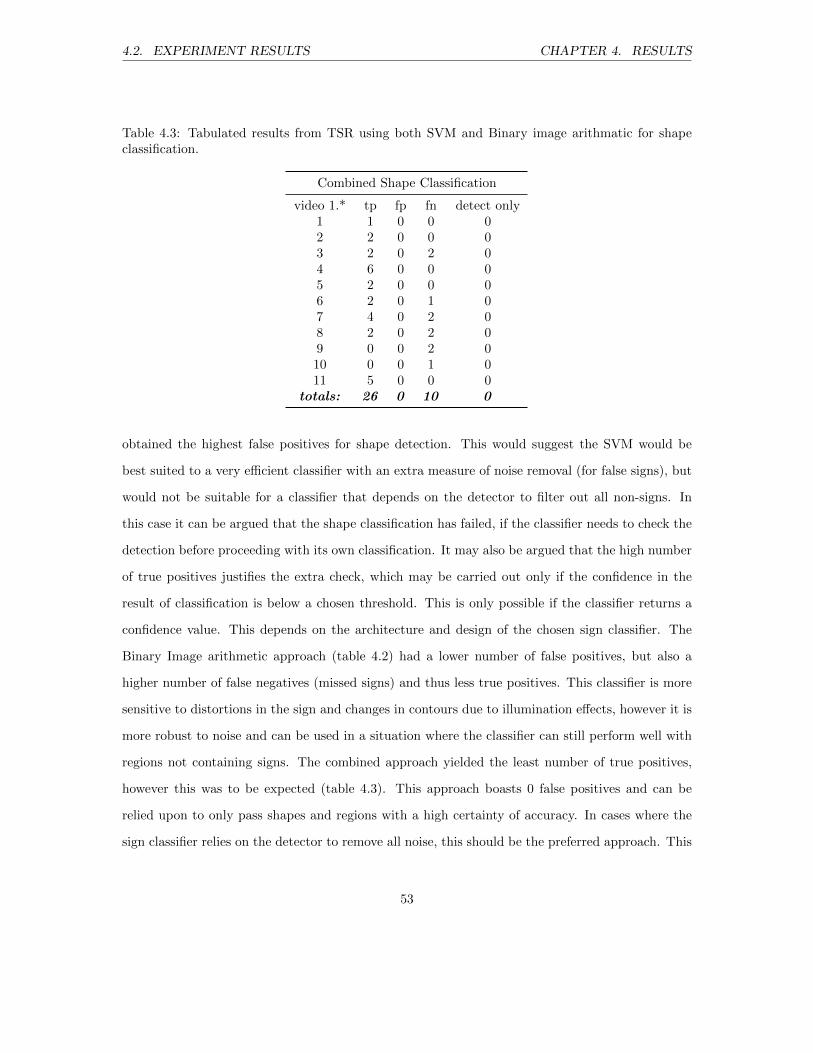
4.2. EXPERIMENT RESULTS CHAPTER 4. RESULTS
Table 4.3: Tabulated results from TSR using both SVM and Binary image arithmatic for shapeclassification.
Combined Shape Classification
video 1.* tp fp fn detect only1 1 0 0 02 2 0 0 03 2 0 2 04 6 0 0 05 2 0 0 06 2 0 1 07 4 0 2 08 2 0 2 09 0 0 2 010 0 0 1 011 5 0 0 0
totals: 26 0 10 0
obtained the highest false positives for shape detection. This would suggest the SVM would be
best suited to a very efficient classifier with an extra measure of noise removal (for false signs), but
would not be suitable for a classifier that depends on the detector to filter out all non-signs. In
this case it can be argued that the shape classification has failed, if the classifier needs to check the
detection before proceeding with its own classification. It may also be argued that the high number
of true positives justifies the extra check, which may be carried out only if the confidence in the
result of classification is below a chosen threshold. This is only possible if the classifier returns a
confidence value. This depends on the architecture and design of the chosen sign classifier. The
Binary Image arithmetic approach (table 4.2) had a lower number of false positives, but also a
higher number of false negatives (missed signs) and thus less true positives. This classifier is more
sensitive to distortions in the sign and changes in contours due to illumination effects, however it is
more robust to noise and can be used in a situation where the classifier can still perform well with
regions not containing signs. The combined approach yielded the least number of true positives,
however this was to be expected (table 4.3). This approach boasts 0 false positives and can be
relied upon to only pass shapes and regions with a high certainty of accuracy. In cases where the
sign classifier relies on the detector to remove all noise, this should be the preferred approach. This
53

4.2. EXPERIMENT RESULTS CHAPTER 4. RESULTS
combined approach has been compared to the cascade classifier and the results will be discussed in
section 4.2.2.
Tracking
The tracking system facilitates voting. It adds reliability to shape classifications because the more
votes a shape has, the more likely that shape is correct. The tracking system implemented in this
approach performed well, however there are areas where improvements could be made. Adding a
weighting scheme based on the signs proximity will improve accuracy because classification of signs
in the distance are less reliable. This is due to distant signs being represented by fewer pixels. Giving
distant signs less weight than closer signs means reliable votes will carry more weight. Another area
for weakness is present because tracking (and thus voting) is connected to an (x,y) position in the
image. When two signs occupy close positions or cross over, the voting scheme may cast votes
to the wrong signs. This potential source for error was not handled in this approach because the
likelihood of signs occupying or crossing the same position over multiple frames is low. Also, the
signs would receive individual votes again when they moved away from each other, so increasing
the number of votes before classification would reduce the likelihood of this error.
4.2.2 Comparison between the Proposed System and Cascade Classifier
Detection
The overall comparison for traffic sign detection will be covered in this section. The detection
is the focus of this report and the next step being sign classification is beyond the scope of this
research. In the discussion, the ”next step” will refer to passing the region of interest onto the
classifier. Popular classification approaches have been briefly covered in section 2.4.2. The table
4.4 shows the tabulated results from Video 1 and Video 2 for each traffic sign detection approach;
combined Cascade classifier, multiple Cascade Classifiers and the Proposed approach. The combined
classifier does not give feedback on the signs shape and the corresponding elements in the table
have therefore been left out. It can be seen in the table 4.4 that the Multiple Cascades had the
highest classification accuracy with 100 %. This shows very reliable feedback on shape for the
54

4.2. EXPERIMENT RESULTS CHAPTER 4. RESULTS
Table 4.4: Final Sign Detection test results. Test Video 2 uses a different camera from training,and contains segments with difficult lighting conditions.
Test Video 1
36 signs Multiple Cascades Single Cascade Proposed
signs detected 17 13 33detection rate(%) 47 36 92
shapes detected 17 . 25correct shape classification 17 . 24shape classification accuracy(%) 100 . 96
Test Video 2
25 signs
signs detected 15 13 2detection rate(%) 60 52 8
shapes detected 15 . 2correct shape classification 13 . 2shape classification accuracy(%) 87 . 100
55
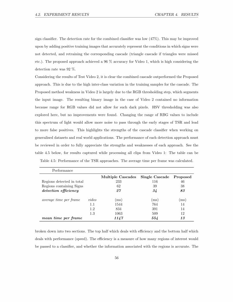
4.2. EXPERIMENT RESULTS CHAPTER 4. RESULTS
sign classifier. The detection rate for the combined classifier was low (47%). This may be improved
upon by adding positive training images that accurately represent the conditions in which signs were
not detected, and retraining the corresponding cascade (triangle cascade if triangles were missed
etc.). The proposed approach achieved a 96 % accuracy for Video 1, which is high considering the
detection rate was 92 %.
Considering the results of Test Video 2, it is clear the combined cascade outperformed the Proposed
approach. This is due to the high inter-class variation in the training samples for the cascade. The
Proposed method weakness in Video 2 is largely due to the RGB thresholding step, which segments
the input image. The resulting binary image in the case of Video 2 contained no information
because range for RGB values did not allow for such dark pixels. HSV thresholding was also
explored here, but no improvements were found. Changing the range of RBG values to include
this spectrum of light would allow more noise to pass through the early stages of TSR and lead
to more false positives. This highlights the strengths of the cascade classifier when working on
generalised datasets and real world applications. The performance of each detection approach must
be reviewed in order to fully appreciate the strengths and weaknesses of each approach. See the
table 4.5 below, for results captured while processing all clips from Video 1: The table can be
Table 4.5: Performance of the TSR approaches. The average time per frame was calculated.
Performance
Multiple Cascades Single Cascade ProposedRegions detected in total 233 116 46Regions containing Signs 62 39 38detection efficiency 27 34 83
average time per frame video (ms) (ms) (ms)1.1 1544 764 141.2 834 391 141.3 1063 509 12
mean time per frame 1147 554 13
broken down into two sections. The top half which deals with efficiency and the bottom half which
deals with performance (speed). The efficiency is a measure of how many regions of interest would
be passed to a classifier, and whether the information associated with the regions is accurate. The
56

4.2. EXPERIMENT RESULTS CHAPTER 4. RESULTS
Multiple Cascades Classifier detected a total of 233 regions that were thought to contain signs. Of
these 233, 62 actually contained signs and this led to a detection efficiency of 27 %. The detection of
the combined (single) cascade showed improved efficiency with 34 %, passing a total of 116 regions
onto the next step. The proposed system only passed 46 regions onto the next step, 38 of these
contained a sign. This led to a high efficiency of 83 %. The efficiency of a detector is important
when working with mobile computation systems, as power and processing capabilities are limited
in such cases. The resources are focused on the classification for large structures such as Neural
nets and high dimensional SVM classifiers.
The performance gives insight into the constraints imposed on a classifier by the detector. If the
detector requires 1 second to process a frame, the classification may need to run on less than a
frame per second. The results from the lower half of table 4.5 show the average time taken for
the detection to process a single frame. The multiple cascades approach, which had the lowest
efficiency, also had the slowest performance. This is expected as multiple cascades were required to
give feedback on shape. The single cascade could detect signs at just less than 2 frames per second.
This is an improvement from using multiple cascades, but without feedback on the shape, the sign
classification would be less efficient. This is because the classification would need to make decisions
on the entire sign dataset, and not just in a sub-group of signs for a particular shape. The proposed
approach achieved the best performance with a mean time per frame of 13 ms. This means that
with the current computational constraints, it could detect signs in video at just over 76 frames per
second, 88 times faster than the multiple cascades approach.
The proposed method has better performance and shape classification accuracy than both Cascade
Classifier approaches. The method would need to be adapted for changing illumination conditions
however, as was highlighted in test video 2.
57

Chapter 5
Conclusion
In this study, an efficient approach to traffic sign detection from a moving vehicle has been pro-
posed. The approach uses RGB thresholding and determines regions of interest using contours. The
approach combines close contours to allow for early recognition and tracks features over multiple
frames to facilitate shape classification voting. The detector determines a signs shape using two
methods of classification that form redundancy and improve accuracy. The shape classification is
achieved using a Support Vector Machine and a binary image arithmetic combination. The pro-
posed algorithms have been evaluated in two videos during daylight conditions using a GoPro 2
camera mounted on the front of a motor vehicle.
Three main experiments were carried out. The first experiment measured the accuracy of the SVM
and the Binary Image Arithmetic approaches for a signs shape classification. The second experiment
determined the recognition rates of a Cascade Classifier trained with all sign shapes to a series of
Cascade Classifiers trained with unique shapes, and the proposed performance approach. The third
experiment determined the performance of each of the three approaches used in experiment 2.
The results showed that the proposed approach is more reliable to pass on shape with fewer false
positives in constrained lighting conditions. The proposed approach outperformed the Cascade
detection in all test cases in terms of computation, and would be ideally suited to a low-power
mobile detection unit. The Cascade Classifier detection method proved to be more robust to other
58

CHAPTER 5. CONCLUSION
lighting conditions, however the performance would limit its accuracy in low power scenarios. This
is due to the number of frames that would need to be skipped for the approach to run in real-time.
In cases where the vehicle is moving at high velocity such as on free-ways, information may be
missed if the camera frame rate is low, or frames need to be skipped for real-time processing.
Future improvements on the proposed method
In order to improve on the proposed approach, a segmentation algorithm that is more robust to
changing lighting conditions must be implemented. The RGB thresholding implementation fails in
low contrast situations and low illumination. When the light source is behind the sign, its shadow
makes the signs red pixels harder to detect and segment. This segmentation is vital to a successful
detection and shape classification, and in the cases where the proposed approach failed, this was
the underlying cause. One possible solution may include determining the scenes global lighting
conditions in a given frame. Once the illumination conditions have been determined, the system
may apply different threshold values, or colour transformations that are best suited to those specific
conditions.
The shape classification may be improved by adding more linearly independent features to SVM im-
plementation. The Binary Image Arithmetic (BIA) shape classification approach may be improved
by applying transformations to input images before carrying out the arithmetic. By stretching the
exterior edges of objects in the binary images to better fit the frame, templates will be more effec-
tive at determining shape because edges would always be present along expected edges. Another
possible approach to determine shape may be to use the plot of the distance from the edge of a
shape to its centroid, as proposed by Khan et al. [2011]. This could then be used as a feature in the
SVM, and the image arithmetic step may be discarded, potentially further improving computation
performance as well as shape classification accuracy. The Cascade Classification detection rate may
be improved by retraining the detector with negative images that contain features which caused
false positives during testing.
59

Bibliography
The german traffic sign recognition benchmark, 2012. URL http://benchmark.ini.rub.de/.
Accessed: 2015-03-25.
ASIRT. Annual global road crash statistics, 2014.
Mohamed Benallal and Jean Meunier. Real-time color segmentation of road signs. In Electrical and
Computer Engineering, 2003. IEEE CCECE 2003. Canadian Conference on, volume 3, pages
1823–1826. IEEE, 2003.
Christopher M Bishop. Pattern recognition and machine learning, ser. Information science and
statistics. Springer, page 15, 2006.
Fabio Boi and Lorenzo Gagliardini. A support vector machines network for traffic sign recognition.
In Neural Networks (IJCNN), The 2011 International Joint Conference on, pages 2210–2216.
IEEE, 2011.
G. Bradski. Dr. Dobb’s Journal of Software Tools.
Alberto Broggi, Pietro Cerri, Paolo Medici, Pier Paolo Porta, and Guido Ghisio. Real time road
signs recognition. In Intelligent Vehicles Symposium, 2007 IEEE, pages 981–986. IEEE, 2007.
Dan Ciresan, Ueli Meier, Jonathan Masci, and Jurgen Schmidhuber. Multi-column deep neural
network for traffic sign classification. Neural Networks, 32:333–338, 2012.
60

BIBLIOGRAPHY BIBLIOGRAPHY
Dan C Ciresan, Ueli Meier, Jonathan Masci, Luca Maria Gambardella, and Jurgen Schmidhuber.
Flexible, high performance convolutional neural networks for image classification. In IJCAI
Proceedings-International Joint Conference on Artificial Intelligence, volume 22, page 1237, 2011.
Dan Claudiu Ciresan, Ueli Meier, Luca Maria Gambardella, and Jurgen Schmidhuber. Deep, big,
simple neural nets for handwritten digit recognition. Neural Computation, 22(12):3207–3220,
2010.
Nello Cristianini and John Shawe-Taylor. An introduction to support vector machines and other
kernel-based learning methods. Cambridge university press, 2000.
Kenneth Dawson-Howe. A Practical Introduction to Computer Vision with OpenCV. John Wiley
& Sons, 2014.
Arturo De La Escalera, Luis E Moreno, Miguel Angel Salichs, and Jose Marıa Armingol. Road
traffic sign detection and classification. Industrial Electronics, IEEE Transactions on, 44(6):
848–859, 1997.
Leonardo Estevez and Nasser Kehtarnavaz. A real-time histographic approach to road sign recog-
nition. In Proceedings of the IEEE southwest symposium on image analysis and interpretation,
pages 95–100, 1996.
Hasan Fleyeh and Mark Dougherty. Road and traffic sign detection and recognition. In Proceedings
of the 16th Mini-EURO Conference and 10th Meeting of EWGT, pages 644–653, 2005.
Meng-Yin Fu and Yuan-Shui Huang. A survey of traffic sign recognition. In Wavelet Analysis and
Pattern Recognition (ICWAPR), 2010 International Conference on, pages 119–124. IEEE, 2010.
Kevin Jarrett, Koray Kavukcuoglu, Marc’Aurelio Ranzato, and Yann LeCun. What is the best
multi-stage architecture for object recognition? In Computer Vision, 2009 IEEE 12th Interna-
tional Conference on, pages 2146–2153. IEEE, 2009.
Robert Kastner, Thomas Michalke, Thomas Burbach, Jannik Fritsch, and Christian Goerick.
61

BIBLIOGRAPHY BIBLIOGRAPHY
Attention-based traffic sign recognition with an array of weak classifiers. In Intelligent Vehi-
cles Symposium (IV), 2010 IEEE, pages 333–339. IEEE, 2010.
Jesmin F Khan, Sharif Bhuiyan, and Reza R Adhami. Image segmentation and shape analysis
for road-sign detection. Intelligent Transportation Systems, IEEE Transactions on, 12(1):83–96,
2011.
Davis E. King. Dlib-ml: A machine learning toolkit. Journal of Machine Learning Research, 10:
1755–1758, 2009.
Sergio Lafuente-Arroyo, Sancho Salcedo-Sanz, Saturnino Maldonado-Bascon, Jose Antonio Portilla-
Figueras, and Roberto Javier Lopez-Sastre. A decision support system for the automatic manage-
ment of keep-clear signs based on support vector machines and geographic information systems.
Expert Systems with Applications, 37(1):767–773, 2010.
Robert Laganiere. OpenCV 2 Computer Vision Application Programming Cookbook: Over 50 recipes
to master this library of programming functions for real-time computer vision. Packt Publishing
Ltd, 2011.
Yann LeCun, Koray Kavukcuoglu, and Clement Farabet. Convolutional networks and applications
in vision. In Circuits and Systems (ISCAS), Proceedings of 2010 IEEE International Symposium
on, pages 253–256. IEEE, 2010.
Rainer Lienhart, Alexander Kuranov, and Vadim Pisarevsky. Empirical analysis of detection cas-
cades of boosted classifiers for rapid object detection. In Pattern Recognition, pages 297–304.
Springer, 2003.
MATLAB. version 7.10.0 (R2010a). The MathWorks Inc., Natick, Massachusetts, 2010.
Ueli Meier, Dan Claudiu Ciresan, Luca Maria Gambardella, and Jurgen Schmidhuber. Better
digit recognition with a committee of simple neural nets. In Document Analysis and Recognition
(ICDAR), 2011 International Conference on, pages 1250–1254. IEEE, 2011.
62

BIBLIOGRAPHY BIBLIOGRAPHY
Andreas Møgelmose, Mohan Manubhai Trivedi, and Thomas B Moeslund. Vision-based traffic
sign detection and analysis for intelligent driver assistance systems: Perspectives and survey.
Intelligent Transportation Systems, IEEE Transactions on, 13(4):1484–1497, 2012.
Avinash N. Ho Gi Jung Hyuckmin Na Monika Singh, Dev Dutt Yadav. Traffic sign recognition-based
vehicle speed regulation. 2009.
World Health Organization et al. WHO global status report on road safety 2013: supporting a
decade of action. World Health Organization, 2013.
Andrzej Ruta, Yongmin Li, and Xiaohui Liu. Real-time traffic sign recognition from video by
class-specific discriminative features. Pattern Recognition, 43(1):416–430, 2010.
Andrzej Ruta, Fatih Porikli, Shintaro Watanabe, and Yongmin Li. In-vehicle camera traffic sign
detection and recognition. Machine Vision and Applications, 22(2):359–375, 2011.
Pierre Sermanet and Yann LeCun. Traffic sign recognition with multi-scale convolutional networks.
In Neural Networks (IJCNN), The 2011 International Joint Conference on, pages 2809–2813.
IEEE, 2011.
Radu Timofte, Karel Zimmermann, and Luc Van Gool. Multi-view traffic sign detection, recogni-
tion, and 3d localisation. Machine Vision and Applications, 25(3):633–647, 2014.
Paul Viola. Robust real-time object detection. paul viola, michael jones, robust real-time object
detection. International Journal of Computer Vision, 2001.
63