road lane and traffic sign detection & tracking for ... · road lane and traffic sign detection...
TRANSCRIPT

ROAD LANE AND TRAFFIC SIGN DETECTION & TRACKING FOR
AUTONOMOUS URBAN DRIVING
by
M. Caner Kurtul
B.S. in Computer Engineering, Bogazici University, 2000
Submitted to the Institute for Graduate Studies in
Science and Engineering in partial fulfillment of
the requirements for the degree of
Master of Science
Graduate Program in Computer Engineering
Bogazici University
2010
ii
ROAD LANE AND TRAFFIC SIGN DETECTION & TRACKING FOR
AUTONOMOUS URBAN DRIVING
APPROVED BY:
Prof. H. Levent Akın . . . . . . . . . . . . . . . . . . .
(Thesis Supervisor)
Prof. Oguz Tosun . . . . . . . . . . . . . . . . . . .
Assoc. Prof. Tankut Acarman . . . . . . . . . . . . . . . . . . .
DATE OF APPROVAL:

iii
ACKNOWLEDGEMENTS
First, I would like to thank my supervisor Professor H. Levent Akın for his guid-
ance. This thesis would not have been possible without his encouragement and enthu-
siastic support.
I would also like to thank all the staff at the Artificial Intelligence Laboratory
for their encouragement throughout the year. Their success in RoboCup is always a
good motivation. Sharing their precious ideas during the weekly seminars have always
guided me to the right direction.
Finally I am deeply grateful to my family and to my wife Derya. They always give
me endless love and support, which has helped me to overcome the various challenges
along the way. Thank you for your patience...
iv
ABSTRACT
ROAD LANE AND TRAFFIC SIGN DETECTION &
TRACKING FOR AUTONOMOUS URBAN DRIVING
The field of Intelligent Transport Systems (ITS) is improving rapidly in the world.
Ultimate aim of such systems is to realize fully autonomous vehicle. The researches
in the field offer the potential for significant enhancements in safety and operational
efficiency.
Lane tracking is an important topic in autonomous navigation because the naviga-
ble region usually stands between the lanes, especially in urban environments. Several
approaches have been proposed, but Hough transform seems to be the dominant among
all. A robust lane tracking method is also required for reducing the effect of the noise
and achieving the required processing time. In this study, we present a new lane track-
ing method which uses a partitioning technique for obtaining Multiresolution Hough
Transform (MHT) of the acquired vision data. After the detection process, a Hidden
Markov Model (HMM) based method is proposed for tracking the detected lanes.
Traffic signs are important instruments to indicate the rules on roads. This makes
them an essential part of the ITS researches. It is clear that leaving traffic signs out of
concern will cause serious consequences. Although the car manufacturers have started
to deploy intelligent sign detection systems on their latest models, the road conditions
and variations of actual signs on the roads require much more robust and fast detection
and tracking methods. Localization of such systems is also necessary because traffic
signs differ slightly between countries. This study also presents a fast and robust
sign detection and tracking method based on geometric transformation and genetic
algorithms (GA). Detection is done by a genetic algorithm (GA) approach supported
by a radial symmetry check so that false alerts are considerably reduced. Classification

v
is achieved by a combination of SURF features with NN or SVM classifiers. A heuristic
alternative to the SURF usage is also presented. Time and accuracy analysis can be
found in relevant sections.
This work is a part of the Automatic Driver Evaluation System (ADES) Project
in Artificial Intelligence Laboratory of Bogazici University.

vi
OZET
YOL SERITLERI / TRAFIK TABELASI TESPIT VE
TAKIBI
Akıllı Tasıma Sistemleri uzerine arastırmalar hızla ilerlemekte. Bu sistemlerin
nihai amacı tamamen otonom aracları gercek hale getirmek. Bu alandaki arastırmalar,
hem guvenlik ve hem de operasyonel verimlilik acılarından onemli potansiyel arz ediyor.
Serit takibi, otonom arac seyri (navigasyon) onemli bir parcası olarak one cıkıyor.
Bunun nedeni, seyredilecek yolun, ozellikle kentsel yollarda, seritler arasındaki bolge
olması. Bu amacla bircok bilimsel yaklasım ileri surulmekle birlikte, bunların arasında
Hough donusumu one cıkmakta. Verideki gurultuyu azaltmak ve sınırlı islem suresinde
sonuca ulasmak icin saglam bir metod tasarlamak gerekiyor. Bu calısmamızda resmi
bolumlere ayırmak kaydıyla Cok Asamalı Hough Donusumu gerceklestiren bir serit
takip sistemi sunuyoruz. Serit tespit asamasının ardından Saklı Markov Modeli temelli
bir serit takip sistemi oneriliyor.
Trafik tabelaları ise yollardaki kuralları belirten onemli enstrumanlardır. Bu
sebeple otonom arac calısamalarının onemli parcasıdırlar. Tabelaların kapsam dısı
bırakılması gercekci sonuclar alınmasını imkansız kılacaktır. Otomotiv uretici firmaları
yeni modellerinde trafik tabelası tanıyabilen akıllı sistemler sunmaya basladılar. Fakat
yollardaki beklenmedik durumlar ve tabelaların onemli farklılıklar gostermesi sebebiyle
cok daha guvenli ve hızlı tabela tanıma sistemlerine ihtiyac duyuluyor. Bu sistem-
ler icin yerellestirme de gerekli cunku trafik tabelaları ulkeden ulkeye farklılıklar arz
edebilmekte. Bu calısmamızda tabela tespit ve takibi icin de bir yontem sunmak-
tayız. Radyal simetri tabanlı geometrik donusumler ve genetik algoritma kullanarak
tabelaları tespit ediyoruz. Tespit edilen tabelalar, SURF niteliklerini Yapay Sinir Agları
veya Destek Vektor Makinelerine besleyerek sınıflandırılıyor. SURF’a alternatif olarak

vii
bir sezgisel bir yontem de deneniyor. Zaman ve dogruluk analizleri ilgili bolumlerede
bulunabilir.
Bu calısma Bogazici Universitesi Yapay Zeka Laboratuvarı’nda yurutulen Otonom
Surus Degerlendirme Projesi’nin bir parcası olarak ortaya cıkmıstır.
viii
TABLE OF CONTENTS
ACKNOWLEDGEMENTS . . . . . . . . . . . . . . . . . . . . . . . . . . . . . iii
ABSTRACT . . . . . . . . . . . . . . . . . . . . . . . . . . . . . . . . . . . . . iv
OZET . . . . . . . . . . . . . . . . . . . . . . . . . . . . . . . . . . . . . . . . . vi
LIST OF FIGURES . . . . . . . . . . . . . . . . . . . . . . . . . . . . . . . . . xi
LIST OF TABLES . . . . . . . . . . . . . . . . . . . . . . . . . . . . . . . . . . xiv
LIST OF ABBREVIATIONS . . . . . . . . . . . . . . . . . . . . . . . . . . . . xv
1. INTRODUCTION . . . . . . . . . . . . . . . . . . . . . . . . . . . . . . . . 1
1.1. Motivation . . . . . . . . . . . . . . . . . . . . . . . . . . . . . . . . . . 2
1.2. Approach and Contributions . . . . . . . . . . . . . . . . . . . . . . . . 3
1.3. Outline of the Thesis . . . . . . . . . . . . . . . . . . . . . . . . . . . . 5
2. LITERATURE REVIEW . . . . . . . . . . . . . . . . . . . . . . . . . . . . 1
2.1. Lane Detection and Tracking . . . . . . . . . . . . . . . . . . . . . . . 1
2.1.1. Randomized Hough Transform for Lane Detection . . . . . . . . 1
2.1.2. Multiresolution Hough Transform for Lane Detection . . . . . . 2
2.1.3. VioLET: Steerable Filters based Lane Detection . . . . . . . . . 3
2.1.4. ALVINN: Autonomous Land Vehicle In a Neural Network . . . 3
2.1.5. Lane Segmentation Using Dynamic Programming . . . . . . . . 4
2.1.6. Lane Detection Using B-Snake . . . . . . . . . . . . . . . . . . . 5
2.1.7. LOIS: Likelihood of Image Shape . . . . . . . . . . . . . . . . . 5
2.1.8. Lane Tracking with LOIS . . . . . . . . . . . . . . . . . . . . . 6
2.1.9. Lane Tracking Using Particle Filtering . . . . . . . . . . . . . . 6
2.1.10. Deformable Template Model Approach to Lane Tracking . . . . 7
2.1.11. General Obstacle and Lane Detection (GOLD) . . . . . . . . . . 8
2.1.12. Stochastic Resonance Based Noise Utilization for Lane Detection 8
2.1.13. Kalman Filters for Curvature Estimation . . . . . . . . . . . . . 8
2.1.14. Adaptive Random Hough Transform for Lane Tracking . . . . . 9
2.1.15. Extended Hyperbola Model for Lane Detection . . . . . . . . . 9
2.1.16. SVM Based Lane Change Detection . . . . . . . . . . . . . . . . 10
2.2. Sign Detection and Classification . . . . . . . . . . . . . . . . . . . . . 10

ix
2.2.1. Neural Networks for Sign Classification . . . . . . . . . . . . . . 10
2.2.2. Kalman Filters for Traffic Sign Detection and Tracking . . . . . 11
2.2.3. Sign Detection Using AdaBoost and Haar Wavelet Features . . 12
2.2.4. Matching Pursuit (MP) Algorithm for Traffic Sign Recognition . 12
2.2.5. Shape-based Road Sign Detection . . . . . . . . . . . . . . . . . 13
2.2.6. Support Vector Machine Approaches for Traffic Sign Detection
and Classification . . . . . . . . . . . . . . . . . . . . . . . . . . 13
2.2.7. Genetic Algorithm for Traffic Sign Detection . . . . . . . . . . . 15
2.2.8. Traffic Sign Classification Using Ring Partitioned Method . . . 15
2.2.9. Recognition of Traffic Signs Using Human Vision Models . . . . 16
2.2.10. Road and Traffic Sign Color Detection and Segmentation-A Fuzzy
Approach . . . . . . . . . . . . . . . . . . . . . . . . . . . . . . . 16
2.2.11. Recognition of Traffic Signs With Two Camera System . . . . . 17
2.2.12. Hough Transform for Traffic Sign Detection . . . . . . . . . . . 17
2.2.13. Class-specific Discriminative Features and Kalman Filter for Sign
Detection and Classification . . . . . . . . . . . . . . . . . . . . 18
3. LANE DETECTION AND TRACKING . . . . . . . . . . . . . . . . . . . . 20
3.1. Methodology . . . . . . . . . . . . . . . . . . . . . . . . . . . . . . . . 20
3.1.1. Hough Transform Overview . . . . . . . . . . . . . . . . . . . . 20
3.1.2. Detection: Multiresolution Hough Transform (MHT) . . . . . . 21
3.1.3. Tracking: HMM . . . . . . . . . . . . . . . . . . . . . . . . . . . 23
3.2. Experiments and Results . . . . . . . . . . . . . . . . . . . . . . . . . . 25
3.2.1. Setup . . . . . . . . . . . . . . . . . . . . . . . . . . . . . . . . 25
3.2.2. Results . . . . . . . . . . . . . . . . . . . . . . . . . . . . . . . . 27
4. SIGN DETECTION AND TRACKING . . . . . . . . . . . . . . . . . . . . 30
4.1. Methodology . . . . . . . . . . . . . . . . . . . . . . . . . . . . . . . . 31
4.1.1. Image Binarization . . . . . . . . . . . . . . . . . . . . . . . . . 32
4.1.2. GA Learning . . . . . . . . . . . . . . . . . . . . . . . . . . . . 35
4.1.3. Modified Radial Symmetry . . . . . . . . . . . . . . . . . . . . . 40
4.1.4. Brightness Correction . . . . . . . . . . . . . . . . . . . . . . . 41
4.1.5. Generic Color Labeler . . . . . . . . . . . . . . . . . . . . . . . 43
4.1.6. Sign Extraction . . . . . . . . . . . . . . . . . . . . . . . . . . . 44
x
4.2. Experiments and Results . . . . . . . . . . . . . . . . . . . . . . . . . . 45
5. SIGN CLASSIFICATION . . . . . . . . . . . . . . . . . . . . . . . . . . . . 48
5.1. Methodology . . . . . . . . . . . . . . . . . . . . . . . . . . . . . . . . 48
5.1.1. Center of Mass (CoM) . . . . . . . . . . . . . . . . . . . . . . . 48
5.1.2. Feature Extraction: 12x12 Occupancy Grid . . . . . . . . . . . 49
5.1.3. Feature Extraction: SURF Interest Points . . . . . . . . . . . . 50
5.1.4. Classification: NN-based . . . . . . . . . . . . . . . . . . . . . . 57
5.1.5. Classification: SVM-based . . . . . . . . . . . . . . . . . . . . . 59
5.2. Experiments and Results . . . . . . . . . . . . . . . . . . . . . . . . . . 61
6. CONCLUSIONS . . . . . . . . . . . . . . . . . . . . . . . . . . . . . . . . . 64
APPENDIX A: VIDEO CAPTURING SYSTEM . . . . . . . . . . . . . . . . 66
APPENDIX B: APPLICATION CONSOLE OF ADES . . . . . . . . . . . . . 67
APPENDIX C: WARNING SIGNS IN TURKEY . . . . . . . . . . . . . . . . 68
APPENDIX D: REGULATORY SIGNS IN TURKEY . . . . . . . . . . . . . 69
APPENDIX E: PROHIBITION SIGNS IN TURKEY . . . . . . . . . . . . . . 70
APPENDIX F: INFORMATIONAL SIGNS IN TURKEY . . . . . . . . . . . 71
REFERENCES . . . . . . . . . . . . . . . . . . . . . . . . . . . . . . . . . . . . 72

xi
LIST OF FIGURES
Figure 1.1. Basic system architecture of ADES project. . . . . . . . . . . . . . 3
Figure 3.1. Liner Hough transform. . . . . . . . . . . . . . . . . . . . . . . . . 21
Figure 3.2. Block Diagram for Multiresolution HT. . . . . . . . . . . . . . . . 22
Figure 3.3. (a) Partitioned image, (b) Binary image. . . . . . . . . . . . . . . 23
Figure 3.4. (a) Candidate lines, (b) Transformed line, (c) Detected lines. . . . 23
Figure 3.5. Hidden Markov Model. (x: states, y: possible observations, a:
state transition probabilities, b: emission probabilities) . . . . . . 24
Figure 3.6. Image partitions. . . . . . . . . . . . . . . . . . . . . . . . . . . . 26
Figure 3.7. Differences between classical Hough transform and proposed ap-
proach. . . . . . . . . . . . . . . . . . . . . . . . . . . . . . . . . . 29
Figure 4.1. Traffic signs used in this study. . . . . . . . . . . . . . . . . . . . . 30
Figure 4.2. Sign detection stages. (a) Original frame, (b) Binarized image,
(c) Triangle verified, (d) Sign extracted, (e) Brightness correction
applied, (f) Detected sign. . . . . . . . . . . . . . . . . . . . . . . 31
Figure 4.3. Good, medium and poor conditions for traffic sign detection. . . . 33
Figure 4.4. Means and standard deviations of sample scene histograms. . . . . 34
Figure 4.5. Original and binarized images with dynamic α, β coefficients. . . . 35
xii
Figure 4.6. Template characteristic points in (x,y) domain, and (u,v) domain
after geometric transformation for circular and triangular signs. . . 38
Figure 4.7. Initial and converged chromosomes. . . . . . . . . . . . . . . . . . 39
Figure 4.8. (a) Circle detection, (b) Scoring of circles. . . . . . . . . . . . . . . 40
Figure 4.9. Candidate circles, and highest score selection. . . . . . . . . . . . 41
Figure 4.10. Detected traffic signs. . . . . . . . . . . . . . . . . . . . . . . . . . 41
Figure 4.11. Candidate triangles, and highest score selection. . . . . . . . . . . 42
Figure 4.12. Brightness correction examples. . . . . . . . . . . . . . . . . . . . 42
Figure 4.13. Generic RGB color labeling algorithm. . . . . . . . . . . . . . . . 43
Figure 4.14. Generic HSL color labeling algorithm. . . . . . . . . . . . . . . . . 43
Figure 4.15. Color labeling examples (black / white). . . . . . . . . . . . . . . 44
Figure 4.16. Extraction of the meaningful part. . . . . . . . . . . . . . . . . . . 45
Figure 5.1. Deviation of CoM from image center. . . . . . . . . . . . . . . . . 49
Figure 5.2. Feature extraction by occupancy grid. . . . . . . . . . . . . . . . . 49
Figure 5.3. Feature extraction in polar coordinates. . . . . . . . . . . . . . . . 50
Figure 5.4. Parameter effects on SURF output. . . . . . . . . . . . . . . . . . 51
Figure 5.5. U-SURF results for different sign types (octaves=3, intervals=5). . 52

xiii
Figure 5.6. Misplacement due to detection step may lead to ambiguities. . . . 53
Figure 5.7. SURF feature extraction. . . . . . . . . . . . . . . . . . . . . . . . 55
Figure 5.8. Segmentation with respect to the CoM. . . . . . . . . . . . . . . . 57
Figure 5.9. a) Biological neurons, b) Artificial neural networks. . . . . . . . . 58
Figure 5.10. SVM feature transform to higher dimensional space. . . . . . . . . 60
Figure A.1. The video camera mounted on the car console. . . . . . . . . . . . 66
Figure B.1. Screenshot of ADES application console. . . . . . . . . . . . . . . 67
xiv
LIST OF TABLES
Table 3.1. Properties of the video sequence. . . . . . . . . . . . . . . . . . . . 25
Table 3.2. Color remapping. . . . . . . . . . . . . . . . . . . . . . . . . . . . 25
Table 3.3. (a) Transmission matrix for r, (b) Transmission matrix for θ. . . . 27
Table 3.4. (a) Emission matrix for r, (b) Emission matrix for θ. . . . . . . . . 28
Table 4.1. Detection rate of circular signs. . . . . . . . . . . . . . . . . . . . . 46
Table 4.2. Detection rate of triangular signs. . . . . . . . . . . . . . . . . . . 47
Table 5.1. NN-train error rates for circular sign classification. . . . . . . . . . 61
Table 5.2. NN-train error rates for triangular sign classification. . . . . . . . . 62
Table 5.3. Classification success rate of circular signs. . . . . . . . . . . . . . 62
Table 5.4. Classification success rate of triangular signs. . . . . . . . . . . . . 63
Table 5.5. Overall system performance. . . . . . . . . . . . . . . . . . . . . . 63

xv
LIST OF ABBREVIATIONS
ADAS Advanced Driver Assistance Systems
ADES Automatic Driver Evaluation System
BMV Behaviour Model of Visions
CoM Center Of Mass
CPU Central Processing Unit
DARPA The Defense Advanced Research Projects Agency
EKF Extended Kalman Filter
EU European Union
FPS Frames per Second
GA Genetic Algorithm
GUI Guided User Interface
HMM Hidden Markov Model
HSL Hue-Saturation-Luminance
HT Hough Transform
ITS Intelligent Transport Systems
LDA Linear Discriminant Analysis
MHT Multi-resolution Hough Transform
MPH Miles per Hour
NN Neural Network
RGB Red Green Blue
ROI Region Of Interest
SIFT Scale-Invariant Feature Transform
SURF Speeded Up Robust Features
SVM Support Vector Machines

1
1. INTRODUCTION
Autonomous driving researches are focused either on off-road driving [1] or driving
in urban traffic [2]. Thanks to the DARPA Grand Challenge and the DARPA Urban
Challenge [3], significant progress have been made in both domains. Autonomous ve-
hicles equipped with several cameras, sensors, and processors prove to move sucessfully
from a starting point to a predefined destination.
There is a remarkable amount of work regarding autonomous driving and its
sub-tasks. Most of these studies target the task of moving the vehicle from one point
to other, just by avoiding collisions and following the most efficient path. This re-
quires optimal path planning and obstacle avoidance algorithms, but not necessarily
the recognition of traffic signs or pedestrians. DARPA Urban Challenge has mandated
some specific rules, most importantly ”lane following”, but has not covered the traffic
rules as a whole. Recognition of traffic lights and signs, and recognition of pedestrians
are officially left out of scope.
Following the progress in this field, car manufacturers have recently started de-
ploying more intelligence in their latest models. Parking assistance, adaptive cruise
control, emergency brake assist, lane departure warning and speed limit monitoring
are among the new features appearing in the car market [4, 5]. All of these systems
are at the very early stages of their evolution. Much more progress is on the horizon.
For example, in the near future, lane, speed limit and traffic light violations are going
to be immediately detected by cars and reported to a central trafic regulation system
with wireless media.
With these expectations in mind, Automatic Driver Evaluation System (ADES)
aims to take a key role in this hot topic of the intelligent car technology. The final
product of the ADES Project will be a framework for evaluating the drivers against
the traffic rules as they drive. It can be used for;

2
• Assisting drivers to drive more safely,
• Informing traffic central about the violations (lane, speed, light, other rules),
• Automation of driver license examinations,
• Highway maintenance: to check the presence and condition of the signs,
• Supervising the development of autonomous urban driving.
This study is a part of the ADES Project and is focused on the road lane and
traffic sign detection and tracking systems. Two different concepts of autonomous
driving challenge are studied and have yielded promising results.
1.1. Motivation
Remarkable amount of the current researches in this field focus on building au-
tonomous driving systems. It seems possible in the future but there seems to be a gap
until the vehicles, drivers and roads become appropriate for fully autonomous vehicles.
Till then, a working solution is required that can be applied in the near future. This
can be a ”Rules Engine” to evaluate how successful a car is being driven.
Such a ”Rules Engine” can have various usage domains. It can be used as a means
for training atonomous vehicles, in real traffic or with traffic simulators. Regarding the
DARPA Urban Challenge vehicles, we can easily say that, they lack a rules engine to
evaluate how successful they navigate in the urban. Our Rules Engine could have been
used as an autonomous referee during the challenge.
Another application area for the ”Rules Engine” can be the collective transporta-
tion vehicles, such as school busses or inter-city coaches. By putting a device on such
vehicles, these vehicles can be observed and drivers can be evaluated more closely and
accurately. Such an option would help drivers to avoid traffic rule violations.
Traffic accidents are one of the main causes of death and economic loss in most of
the developed countries. According to the Road Safety Action Program of European
Commission [6], more than one million accidents a year cause more than 40 000 deaths

3
and nearly two million injuries on the roads. In addition, the direct and indirect cost
has been estimated at 160 billion Euros, which is nearly two percent of the EU’s GNP.
However, the most dramatic fact is that, nearly all of the accidents are caused by
driver mistakes. The main goal of the driver assistance and early warning systems is
to reduce the number of these accidents. However, the performance of such systems
depend on their power to recognize the conditions and rules in the vehicle’s existing
context. Moreover, since most of the rules are expressed by traffic signs, robust and
fast sign detection methods are inevitable for intelligent vehicles.
1.2. Approach and Contributions
The ADES Project can be divided into two major parts (Figure 1.1). The first
part is acquiring the necessary data from various sensors whereas the second part is
processing these data knowledge to evaluate the driver’s actions.
Figure 1.1. Basic system architecture of ADES project.
This thesis is concerned with new approaches for obtaining lane/sign detection
and tracking problems. Regarding the lane detection and tracking issue, this study
introduces a new approach called Multi-resolution Hough Transform (MHT). Lane
markings are detected using MHT and a Hidden Markov Model (HMM) is used for
tracking afterwards.

4
As for the sign detection, this study proposes an approach that encodes the chro-
mosomes of genetic algorithm (GA) by using a geometric transformation matrix. The
fitness function is calculated by a set of transformed points which correspond to the
(triangular or circular) shape of the traffic signs. Afterwards, a modified radial symme-
try check is performed to eliminate the false alerts. The challenge here is that, circular
and triangular signs have entirely diferent geometric features. Therefore two types
of geometric transformation matrices were necessary for the GA fitness computation.
On the other hand radial symmetry check runs in a completely different manner for
the circular and triangular signs. Another challenge is the varying lighting conditions
during a drive. An adaptive brightness correction method is proposed. Depending
on the illumination, the system fine tunes various parameters in order to get a better
detection.
For the classification of the signs, on the other hand, two different approaches are
employed and compared with each other: Neural Networks (NN) and Support Vector
Machines (SVM). The main contribution of this work is to use the U-SURF features for
training NN and SVM. A hybrid approach is adopted for utilizing the U-SURF features.
They are interpreted with respect to the Center of Mass (CoM) of the detected sign.
U-SURF features are compared against a simple heuristic method.
For real-world training, precaptured videos are used. The videos are captured
from a car moving in the urban traffic with a varying velocity. The camera is placed
onto the front console of the car (Appendix A). The captured video has a resolution
of 512x288 pixels with a frame rate of 29.97.
As opposed to the simulated environment, precaptured video sequence provides
noisy data with imperfect lighting conditions. The tests with precaptured video has
shown that, lighting conditions will have major effect on the accuracy of the overall
system.

5
1.3. Outline of the Thesis
The organization of the rest of the thesis is as follows:
In Chapter 2 we summarize the studies relevant to autonomous driving. A de-
tailed analysis is done on the applied methods. This chapter will give an idea on the
algorithms applicable for our purpose.
Chapter 3 details the lane detection methodology and explains how we achieve
the tracking issue. The chapter gives a background for the Hough Transform, Hidden
Markov Model and explains our contribution called Multi-resolution Hough Transform.
Experimental setup and results are also given in detail.
In chapters 4 and 5 we explain our approach on the sign detection and classifi-
cation respectively. Background for the GA, SURF, NN and SVM are given together
with the motivation on selecting them. Experimental runs and results are illustrated
and discussed in detail.
Finally, Chapter 6 concludes the thesis by summarising the contributions and
giving a brief outline of the obtained results. In addition, any shortcomings of the
proposed methods and possible future work are also discussed here.

1
2. LITERATURE REVIEW
2.1. Lane Detection and Tracking
There has been a significant amount of research on vision-based road lane detec-
tion and tracking. Vision-based localization of the lane boundaries can be divided into
two sub-tasks: lane detection and lane tracking.
Lane detection is the problem of locating lane boundaries without prior knowledge
of the road geometry. Most lane detection methods are edge-based. After an edge
detection step, the edge-based methods organize the detected edges into meaningful
structure (lane markings) or fit a lane model to the detected edges. Most of the
edge-based methods, in turn, use straight lines to model the lane boundaries. Others
employed more complex models such as B-Splines, parabola, and hyperbola. With its
ability to detect imperfect instances of the regular shapes, Hough Transform (HT) [7]
is one of the most common techniques used for lane detection. Hough Transform is
a method for detecting lines, curves and ellipses, but in the lane detection literature
it is preferred for its line detection capability. It is mostly employed after an edge
detection step on grayscale images. Besides the Hough Transform, many different
techniques also have been applied for lane detection, such as, neural networks [8],
dynamic programming [9] and deformable template matching [10].
Lane tracking, on the other hand, is the problem of tracking the lane edges from
frame to frame given an existing model of road geometry. Many techniques have been
used for lane tracking. Among them we can mention the Kalman filtering [11], and
particle filtering which are commonly used for modeling the estimation problems.
2.1.1. Randomized Hough Transform for Lane Detection
In [12] Li et al. have proposed a model that uses an adaptive Hough Transform.
The images are first converted into grayscale using only the R and G channels of the

2
color image. They have ignored the B channel relying on the good contrast of red
and green channels with respect to the white and yellow lane markings. The grayscale
image is passed through a very low thresholded Sobel edge detection. Afterwards they
apply a special HT which they call RHT (Randomized HT ). The pixels of RHT are
sampled randomly according to their gradient magnitudes. This method ensures robust
and accurate detection of lane markings especially for noisy images. The 3D Hough
space is reduced to two dimensions for simplifying the problem and reducing the high
computational cost of HT. The experiments have proven better results compared to
GA-based lane detection techniques.
2.1.2. Multiresolution Hough Transform for Lane Detection
In [13] Yu et al. also use Hough Transform to detect the lane boundaries.
This work additionally considers the pavements at the sidewayds. Since the pavement
boundaries are another means of continuous lines, the paper has put special attention
on them. The HT is used to detect lane boundaries with a parabolic model. Road
pavement types, lane structures and weather conditions have carefully been investi-
gated. The 3-D Hough space is decomposed into two sub-domains. A 2-D domain of
parameters shared by all the edge types, and a 1-D domain of remaining distinctive
parameters. This study uses the Canny edge detector to get two images: a binary
image denoting the edges and a gradient image denoting the ratio of vertial and hor-
izontal gradients. They have applied the HT several times from a low resolution to
the desired resolution images. They call this method multiresolution HT, and they
have proven it to reduce the computational cost of classical HT while preserving the
accuracy. The proposed system is only tested with 34 grayscale images of size 256 x
240. The experiments show that the system is capable of handling images of different
qualities, paved and unpaved roads, marked and unmarked roads, shadows, and poor
illumination conditions.
3
2.1.3. VioLET: Steerable Filters based Lane Detection
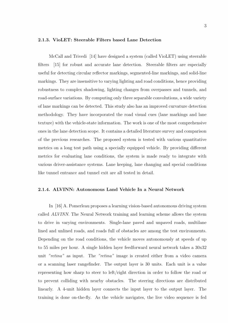
McCall and Trivedi [14] have designed a system (called VioLET) using steerable
filters [15] for robust and accurate lane detection. Steerable filters are especially
useful for detecting circular reflector markings, segmented-line markings, and solid-line
markings. They are insensitive to varying lighting and road conditions, hence providing
robustness to complex shadowing, lighting changes from overpasses and tunnels, and
road-surface variations. By computing only three separable convolutions, a wide variety
of lane markings can be detected. This study also has an improved curvature detection
methodology. They have incorporated the road visual cues (lane markings and lane
texture) with the vehicle-state information. The work is one of the most comprehensive
ones in the lane detection scope. It contains a detailed literature survey and comparison
of the previous researches. The proposed system is tested with various quantitative
metrics on a long test path using a specially equipped vehicle. By providing different
metrics for evaluating lane conditions, the system is made ready to integrate with
various driver-assistance systems. Lane keeping, lane changing and special conditions
like tunnel entrance and tunnel exit are all tested in detail.
2.1.4. ALVINN: Autonomous Land Vehicle In a Neural Network
In [16] A. Pomerleau proposes a learning vision-based autonomous driving system
called ALVINN. The Neural Network training and learning scheme allows the system
to drive in varying environments. Single-lane paved and unpaved roads, multilane
lined and unlined roads, and roads full of obstacles are among the test environments.
Depending on the road conditions, the vehicle moves autonomously at speeds of up
to 55 miles per hour. A single hidden layer feedforward neural network takes a 30x32
unit ”retina” as input. The ”retina” image is created either from a video camera
or a scanning laser rangefinder. The output layer is 30 units. Each unit is a value
representing how sharp to steer to left/right direction in order to follow the road or
to prevent colliding with nearby obstacles. The steering directions are distributed
linearly. A 4-unit hidden layer connects the input layer to the output layer. The
training is done on-the-fly. As the vehicle navigates, the live video sequence is fed
4
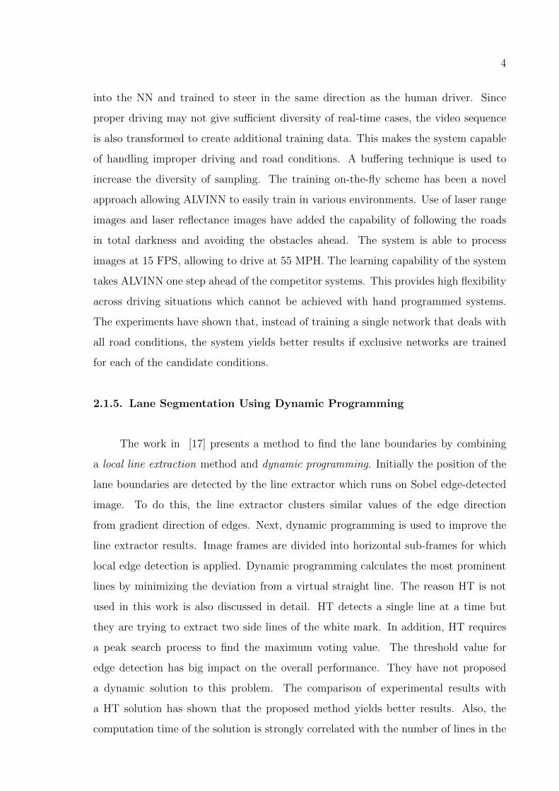
into the NN and trained to steer in the same direction as the human driver. Since
proper driving may not give sufficient diversity of real-time cases, the video sequence
is also transformed to create additional training data. This makes the system capable
of handling improper driving and road conditions. A buffering technique is used to
increase the diversity of sampling. The training on-the-fly scheme has been a novel
approach allowing ALVINN to easily train in various environments. Use of laser range
images and laser reflectance images have added the capability of following the roads
in total darkness and avoiding the obstacles ahead. The system is able to process
images at 15 FPS, allowing to drive at 55 MPH. The learning capability of the system
takes ALVINN one step ahead of the competitor systems. This provides high flexibility
across driving situations which cannot be achieved with hand programmed systems.
The experiments have shown that, instead of training a single network that deals with
all road conditions, the system yields better results if exclusive networks are trained
for each of the candidate conditions.
2.1.5. Lane Segmentation Using Dynamic Programming
The work in [17] presents a method to find the lane boundaries by combining
a local line extraction method and dynamic programming. Initially the position of the
lane boundaries are detected by the line extractor which runs on Sobel edge-detected
image. To do this, the line extractor clusters similar values of the edge direction
from gradient direction of edges. Next, dynamic programming is used to improve the
line extractor results. Image frames are divided into horizontal sub-frames for which
local edge detection is applied. Dynamic programming calculates the most prominent
lines by minimizing the deviation from a virtual straight line. The reason HT is not
used in this work is also discussed in detail. HT detects a single line at a time but
they are trying to extract two side lines of the white mark. In addition, HT requires
a peak search process to find the maximum voting value. The threshold value for
edge detection has big impact on the overall performance. They have not proposed
a dynamic solution to this problem. The comparison of experimental results with
a HT solution has shown that the proposed method yields better results. Also, the
computation time of the solution is strongly correlated with the number of lines in the

5
frames.
2.1.6. Lane Detection Using B-Snake
In [18] Wang et al. have proposed an algorithm based on B-Snake [19]. The
algorithm is able to discover a wider range of lanes, especially the curved ones. B-Snake
is basically a B-Splines implementation, therefore it can form any arbitrary shape by a
set of control points. The system aims to find both sides of lane markings similarly to
[17]. This is achieved by detecting the mid-line of the lane, followed by calculating the
perspective parallel lines. The initial position of the B-snake is decided by an algorithm
called Canny/Hough Estimation of Vanishing Points (CHEVP). The control points are
detected by a minimum energy method.
Snakes [19], or active contours, are curves defined within an image which can
move under the influence of internal forces from the curve itself and external forces
from the image data. This study introduces a novel B-spline lane model with dual
external forces. This has two advantages: First, the computation time is reduced since
two deformation problems is reduced into one; Second, the B-snake model will be more
robust against shadows, noise, and other lighting variations. The overall system is
tested against 50 pre-captured road images with different road conditions. The system
is observed to be robust against noise, shadows, and lighting variations. The approach
has also yielded good results for both the marked and the unmarked roads, and the
dashed and the solid paint line roads.
2.1.7. LOIS: Likelihood of Image Shape
In [20] Kluge and Lakshmanan have introduced the well known LOIS (Likeli-
hood of Image Shape) Lane Detection Algorithm for the first time. Instead of using a
thresholding method they have proposed a deformable template model. Thresholding
is not used since edge-based lane detectors mostly suffer from non-deterministic gradi-
ent magnitude thresholds. Shadows, puddles, tire skid marks and oil stains may create
undesired edges that will require varying threshold values to be filtered out. LOIS also

6
does not require a strict classification as edge and non-edge points. The likelihood
function permits the algorithm to locate the lane edges even when the contrast is poor
or there are many noise edges. LOIS uses the Metropolis algorithm [21] to perform like-
lihood optimization (to identify the optimal set of template deformation parameters).
They have found a set of system parameters that perform well in various road envi-
ronments. The proposed system is shown to perform well at situations where the lane
edges have relatively weak local contrast, or where there are strong distracting edges
due to shadows, puddles and pavement cracks. It seems deformable template model
suits well to the problem, but they may require to replace the Metropolis algorithm
with alternative methods.
2.1.8. Lane Tracking with LOIS
Another study from Kreucher et al. [22] uses the LOIS [20] Lane Detection
Algorithm [23] to track the lanes. The system emits warning messages if a lane crossing
is detected. The vehicle’s location with respect to the lane markings is detected by
LOIS, which uses a deformable template approach. This approach has a parametric
set of shapes that describes all possible ways the object can appear in the image. A
likelihood function is used to measure how well a particular detected object matches
the given image. Previous articles on LOIS focus solely on lane detection where the
vehicle is located around the center of two lanes. This paper’s contribution is using a
Kalman filter to predict the future values of vehicle’s location considering the previously
observed ones. The location is measured in terms of offset values with respect to the
right and left lane markings detected by LOIS. If the vehicle is detected to be within one
meter of either the left or the right lane marking, and if the vehicle’s path, as predicted
by the Kalman filter, will lead it to be within 0.8 meters of either lane markings in less
than one second, then a lane crossing warning is emitted.
2.1.9. Lane Tracking Using Particle Filtering
In [24] Apostoloff and Zelinsky presents the first results from a study where a lane
tracker was developed using particle filtering and visual cue fusion technology. This

7
is part of a work on Australian National University. Several cameras (passive, active,
near-field and far-field coverage) and sensors are located on the vehicle. This research
introduces the first use of particle filtering in a road vehicle application. Another con-
tribution of this study is its ability to automatically adopt to road condition variations
by using a novel Distillation Algorithm which combines a particle filter with a cue fu-
sion engine. This is a notable enhancement compared to the previous researches which
rely on only one or two fixed cues for lane detection that are used regardless of how
well they are performing. Distillation Algorithm on the other hand changes the cues
dynamically considering the variations on the environment. It is based on Bayesian
statistics and is self-optimized to produce the best statistical result. Particle filtering
is also used to track the detected lanes. The lane tracker uses two different sets of cues:
image based cues (lane marker cue, road edge cue, road color cue, non-road color cue)
and the state based cues (road width cue, elastic lane cue). Experiments have shown
that particle filter has impressive results for target detection and tracking. While other
researches use separate procedures for detection and tracking, usage of particle filter
for both tasks have exhibited good results in this study. It also removes the necessity
for additional computations.
2.1.10. Deformable Template Model Approach to Lane Tracking
Similar to LOIS [20, 23, 22] the lane detection approach proposed in [25] uses a
deformable template model. The aim of this study is to overcome problems of Kalman
filter based lane trackers. The problem with the Kalman filter based lane tracking is
that, they cannot recover after a tracking failure occurance. That is because Kalman
filter is based on Gaussian densities which cannot represent simultaneous alternative
hypotheses. In the proposed method the lane boundaries are assumed to be parabolas
in the ground plane. The lane detection is formulated as a ”maximum a posteriori”
(MAP) estimate problem. Tabu search algorithm is used to obtain the global maxima
for the posterior density. The detected lanes are tracked using a particle filter that
recursively estimates the lane shape and the vehicle position. The proposed model
outputs many useful parameters such as the position of the vehicle inside the lane, its
heading direction, and the local structure of the lane.
8
2.1.11. General Obstacle and Lane Detection (GOLD)
The General Obstacle and Lane Detection system (GOLD [26]) used in the
ARGO vehicle at the University of Parma transforms stereo-vision images into a com-
mon bird’s eye view. It uses a pattern matching technique to detect lane markings
on the road. A horizontal search is performed for dark-bright-dark regions of certain
width. The effect of illumination conditions, shadows or sunny blobs is reduced by
considering each pixel not globally but rather with respect to its left and right horizon-
tal neighbors. The road marking pixels mostly have higher brightness value than their
horizontal neighbors. After brightness analysis step a gray-level image is computed
that represents horizontal brightness transitions. This lets use of adaptive threshold
for image binarization. The proposed system is limited to roads with lane markings as
the lane markings form the very basis of the search method.
2.1.12. Stochastic Resonance Based Noise Utilization for Lane Detection
In [27] Bellino et al. present the lane detection techniques used in SPARC (Secure
Propulsion using Advanced Redundant Control) Project financed by EU. This study
introduces two new approaches. First, the noise due to vibration of vehicle can be
used through Stochastic Resonance. While traditional methods try to avoid the noise,
this study uses it to reveal useful information such as the contour of objects and lanes.
Second, this study utilizes several sensors (camera, radar, laser) for lane detection,
whichever is providing reliable data depending on external conditions (shadows, fog,
rain, dark).
2.1.13. Kalman Filters for Curvature Estimation
W. Enkelmann et al. [28] have built a real-time lane tracking system which han-
dles unmarked lane borders as well as marked lane borders. Kalman filter is used for
horizontal and vertical lane curvature estimation. If lane borders are partially occluded
by cars or other obstacles, the results of a completely separate obstacle detection mod-
ule, which utilizes other sensors, are used to increase the robustness of the lane tracking

9
module. They have also given an algorithm to classify the lane types. The illustrated
lane tracking system has two subtasks: departure warning and lane change assistant.
While the lane departure warning system evaluates images from a front looking camera,
the lane change assistant receives signals from back looking cameras and radar sensors.
2.1.14. Adaptive Random Hough Transform for Lane Tracking
A recent study from Zhu et al. [29] presents a novel approach for lane detec-
tion problem. Instead of using one single method to calculate all parameters in the
lane model, the Adaptive Random Hough Transform (ARHT) and the Tabu Search
algorithm are used cooperatively to calculate the different parameters. ARHT is an
efficient approach to detect curves, which determines n parameters of the curve by
sampling n pixels in the edge image. Tabu Search algorithm is based on a ”maximum
a posteriori” (MAP) estimate problem similarly to [25]. A multiresolution strategy
is employed to reduce the execution time and provide more accurate results, similar
to [13]. The proposed system uses a hyperbolic lane model, and therefore is able to
detect both straight and curved lanes. ARHT and Tabu Search are used to calculate
the parameters of the hyperbolic model. Lane tracking is accomplished by a particle
filter. The first frame is used by the detection algorithm. The result of the detection
algorithm is delivered to the particle filter for tracking. Therefore, tracking starts with
the second frame and continues as long as a confidence threshold is satisfied. When
confidence threshold is violated, the detection algorithm is called again to generate new
initial particles for the tracking algorithm.
2.1.15. Extended Hyperbola Model for Lane Detection
Another recent study by Bai et al. [30] uses a different approach for road and
lane detection. An extended hyperbola model is used to represent the road. A non-
linear term is integrated into the model to handle transitions between the straight and
the curved road segments. The parameters of the model are estimated by multiple
vanishing points located on road segments. This paper is primarily focused on road
detection rather than lane detection. But it uses lane information to do so, and presents

10
useful techniques for our intentions.
2.1.16. SVM Based Lane Change Detection
In [30] M. Mandalia and D. Salvucci present an SVM-based method for lane-
change detection. The aim of the proposed system is to detect drivers’ lane change in-
tentions. The technique uses both behavioral and environmental data, but is primarily
focused on behavioral data. Several features are used for SVM training: acceleration,
near-field lane position, far-side lane position, heading, lead car distance, and steering
angle. All SVM kernels have been tested, but linear kernel has performed the best
results. The system was able to detect about 87 percent of all true positives within
the first 0.3 seconds from the start of the maneuver. Usage of lead-car velocity and eye
movements are mentioned to be the future enhancements for the system.
2.2. Sign Detection and Classification
There are numerous methods for the detection and recognition of traffic signs.
Similar to the lane detection algorithms, vision-based sign detection systems also
mostly suffer from adverse weather and lighting conditions. A sign detection system
can be decomposed into two separate parts: detection and classification. Researchers
have proposed various techniques for detection and classification. Among the com-
monly used techniques, we can mention Genetic Algorithms, Neural Networks, Kalman
Filter, radial symmetry, Ada-Boost and LDA.
2.2.1. Neural Networks for Sign Classification
One of the early studies on the topic is introduced by Escalera et al. [31] in
1997. Detection is achieved by a shape analysis on a color thresholded image, whereas
classification is done by neural networks. Although HSI is very invariant to lighting
changes, RGB is preferred in this study. That is because, HSI formulation is nonlin-
ear and therefore requires more processing power. The proposed approach applies a
red-color threshold, followed by corner detector for triangular signs and circumference

11
detector for circular signs. The detectors are basically a set of masks used for convo-
lution. Two separate multilayer perceptron NNs have been trained for triangular and
circular signs. The size of the input layer corresponds to an image of 30x30 pixels, and
the output layer is of size ten, i.e., nine sign types plus one output that shows that the
sign is not one of the nine. Ideal signs were used for training. 1620 training patters
are created out of them by rotating, adding Gaussian noise and displacing 3 pixels.
2.2.2. Kalman Filters for Traffic Sign Detection and Tracking
In [32] Fang et al. have additionally focused on the tracking of the signs through
the image sequence. Prior to tracking phase, they have used two NNs for detecting
the signs: one for color features and one for shape features. A fuzzy approach is used
to create an integration map of the shape and color features, which in turn is used
to detect the signs. To reduce the complexity of detection operations, the system
can only detect signs of a particular size (8-pixel radius). Once the location of the
sign is detected in the current frame, the size and location in the following frame is
predicted by a Kalman filter. This significantly reduces the search space and increases
the accuracy. Nevertheless, the detection technique proposed in this paper requires a
large search space due to the complexity of the integration map.
Piccioli et al. [33] also incorporated both color and edge information to detect
road signs from a single image. They applied the Kalman-filter-based temporal integra-
tion of the extracted information for further improvement. They claimed that to im-
prove the performance, their technique could be applied to temporal image sequences.
In fact, the detection of road signs using only a single image has three problems: 1)
to reduce the search space and time, the positions and sizes of road signs cannot be
predicted; 2) it is difficult to correctly detect a road sign when temporary occlusion
occurs; and 3) the correctness of road signs is hard to verify. By using a video sequence
instead of temporal images, the information from the preceding images, such as the
number of the road signs and their predicted sizes and positions can be preserved. This
information can be used to increase the speed and accuracy of road-sign detection in
subsequent images.

12
2.2.3. Sign Detection Using AdaBoost and Haar Wavelet Features
Bahlmann et al. [34] suggest the use of AdaBoost [35] and Haar wavelet [36] fea-
tures for detection, and a Gaussian probability density model for classification. Tradi-
tional object detection approached generally apply color and shape detection separately
one after the other. Regions that have falsely been rejected by color segmentation, can-
not be recovered in further processing. The main contribution of this paper, with this
motivation, is a joint color and shape modeling within the AdaBoost framework. In
addition, AdaBoost is mostly used to select gray-scale wavelet features specified by
their position, width and height parameters. This study, on the other hand, requires
wavelets to be applied on RGB images. Therefore, instead of gray-scale images, they
have proposed a method to use RGB color images in AdaBoost framework. The overall
system is measured to perform with an error rate of 15 percent.
2.2.4. Matching Pursuit (MP) Algorithm for Traffic Sign Recognition
Hsu and Huang [37] also use a two-fold approach for traffic signs: detection
and recognition. The detection phase, in turn, has three stages. In the first stage, a
region in the captured image where the road sign is more likely to be found is selected.
Here, either the color information or other heuristics (such as possible locations of
road signs, geometrical characteristics of the signs) are used. In the second stage, the
region of interest (ROI) is searched to find the possible location of the triangular or
circular shape regions. Then, a closer view image is captured focusing the identified
regions. In the third stage, template-matching is applied to detect the road signs.
In the recognition phase, matching pursuit (MP) filter [38] is used to recognize the
road signs effectively. Matching pursuit (MP) algorithm uses a greedy heuristic to
iteratively decompose any signal into a linear expansion of waveforms that are selected
from a redundant dictionary of functions. Matching pursuits are general procedures to
compute adaptive signal representations. MP based recognition proposed in this paper
is unfortunately too costly. While the computation time of the detection phase is 100
ms, the recognition operation using matching pursuit method requires about 250 ms.
13
2.2.5. Shape-based Road Sign Detection
Loay and Barnes [39] have developed a time-efficient, rotation-invariant and
shape-based road sign detection technique. It can detect triangular, square and oc-
tagonal road signs. The method uses the symmetric nature of these shapes. Regular
polygons are equiangular i.e., their sides are separated by a regular angular spacing. To
utilize this regularity, they introduce a rotationally invariant measure. However, the
algorithm has an important limitation such that, for each image frame the algorithm
only seeks for predefined radii. Regarding the performance, for a 320x240 image, the
algorithm was able to be run at 20Hz. The approach has strong robustness to varying
illumination as it detects shapes based on edges, and will efficiently reduce the search
for a road sign from the whole image to a small number of pixels. It can detect (without
classification) the signs with a success rate of 95 percent.
2.2.6. Support Vector Machine Approaches for Traffic Sign Detection and
Classification
An SVM-based study introduced by Maldonado et al. [40] can recognize circular,
rectangular, triangular, and octagonal signs. They have used SVM for both detection
and classification purposes. Linear SVMs are used as geometric shape classifiers at
detection phase. They operate on the color-segmented image (red, blue, yellow, white,
or combinations of these colors). After the color segmentation, what is called blobs of
interest (BoI) are detected. Linear SVM executes on these blobs using the distance
to borders (DtBs) as input vectors. For the sign classification phase, on the other
hand, Gaussian-kernel SVMs are used. The input to the recognition stage is a block
of 31x31 pixels in grayscale image for every candidate blob. In order to reduce the
feature vectors, only those pixels that must be a part of the sign (pixels of interest) are
used. The results show a high success rate and a very low amount of false positives in
the final recognition stage. The results reveal that the proposed algorithm is invariant
to translation, rotation, scale, and, in many situations, even to partial occlusions.
This study does not suggest a tracking method. The overall recognition accuracy
of the system is acceptable, and can detect different geometric shapes, i.e., circular

14
and octagonal, and triangular and rectangular. But it requires several performance
enhancements in order to be applicable in real-time. The current computation time is
1.77 seconds per frame.
Another SVM-based solution by Kiran et al. [41] introduces an SVM Learning
technique for traffic sign classification. Similar to many other studies, they have pre-
ferred color segmentation for detection. Only hue and saturation channels are used.
Shape classification is performed using a linear support vector machine. Better shape
classification performance is obtained by training the SVM using novel features called
distance from center (DfC) and distance to borders (DtB). DfC is defined to be the
distance from the center of the blob to the external edge of the blob, whereas, DtB
is distance from the external edge of the blob to its bounding box. Each segmented
blob has four DtB vectors and four DfC vectors for left, right, top and bottom di-
rections. These vectors make the system invariant of translation, rotation and scale
factors. Classification is tested by using DtB alone, and also by combining DtB and
DfC feature vectors. Circular sign classification shows more successful than triangular
ones. Also, joint features usage yields slightly better results. The classification success
rate is around 90 percent, and the true positives rate is around 96 percent.
In [42] Jimenez et al. focus just on the sign detection problem, dividing it into
two sub-blocks that perform shape classification and localization of the sign. This work
is a successor of [40] which used two different SVMs for detection and classification.
The main contribution of this work is basically in the improvement of the detection
block, where the new method developed here has proven to be more successful than
the distance to borders (DtB) method, defined in their previous work [40]. The
classification of the shape is achieved by means of the connected components. Object
rotations are handled with the use of the FFT. The signature of each blob was used for
the classification of the shape of the traffic sign. The normalization of the energy of the
signature makes the algorithm invariant to image scaling, and the use of the absolute
value of the FFT of the normalized signature makes the algorithm invariant to object
rotations. Experimental results, evaluated using a huge set of randomly generated
synthetic images are also given, showing a great robustness to object scaling, rotation,
15
projective deformation, partial occlusions and noise.
2.2.7. Genetic Algorithm for Traffic Sign Detection
A more recent study of Escalera et al. [43] uses genetic algorithm for detection,
and a neural network for classification. The proposed system not only recognizes the
traffic sign but also provides information about its condition or state. Traffic signs are
detected trough color and shape analysis. First the hue and saturation components of
the image are analyzed and the regions in the image that fulfill some color restrictions
are detected. If the area of one of these regions is large enough, a possible sign can be
located in the image. The perimeters of the regions are obtained and a global search of
possible signs is performed with an elitist GA. The initial population of the GA is not
random, but rather is created according to the color analysis results. A thresholding
of the color analysis image is performed and the number and position of the blobs are
obtained. The fitness function is basically the proportion of the number of points whose
distance is less than a threshold value. For NN training, RGB is preferred instead of
HSI, due to HSI’s instability to obtain the hue value of gray colors. Some researches
have used the I component, but the color information would be lost because a dark red
pixel (belonging to the sign border) would have the same value as a dark gray. The NN
is finally followed by an additional sign state analysis step. This helps the algorithm,
not only know the detected sign, but also the confidence in its detection.
2.2.8. Traffic Sign Classification Using Ring Partitioned Method
Soetedjo and Yamada [44] have focused on traffic sign classification using Ring
Partitioned Method on grayscale images. In contrast to the previously discussed meth-
ods, this study does not require many carefully prepared samples for training. In
the pre-processing stage, a special method is used to convert the RGB image into a
grayscale format which is invariant to illumination changes (called ”specified grayscale
image”). First, color thresholding is applied for each of the red, blue, white and black
colors. This produces four grayscale images corresponding to four mentioned colors.
These grayscale images are combined by the ”histogram specification method”, a tech-

16
nique to convert an image into one with particular histogram specified in advance.
The method divides a rectangular ”specified grayscale image” into several rings, which
constitute the ring-partitioned image. A fuzzy histogram value is calculated for each
ring, providing better smoothed values. The Euclidean’s distance is used for match-
ing. It measures the distance between the target image and the reference images. The
proposed system has a matching rate of around 95 percent. But the circular nature of
the rings makes the system applicable only for the circular signs.
2.2.9. Recognition of Traffic Signs Using Human Vision Models
Another different approach [45] is to represent the sign features by using a hu-
man vision color appearance model by Gao et al. CIECAM97 [46] color appearance
model has been applied to extract color information and to segment and classify traffic
signs. CIECAM97 is a standard color appearance model recommended by CIE (Inter-
national Commission on Illumination) in 1997 for measuring color appearance under
various viewing conditions. It takes weather conditions into consideration and simu-
lates human’s perception for perceiving colors under various viewing conditions and for
different media, such as reflection colors, transmissive colors, etc. Only blue and red
signs are used in this study. For the segmentation step, they detect the color ranges
(hue and choroma) for red, blue, black, and white. Based on the range of the sign
colors, traffic sign candidate regions are segmented using quad-tree histogram method.
This will isolate them from the rest of scenes for further processing. Apart from the
color features, the method also applies a method for modeling shape features. Over-
all recognition rate is very high for signs under artificial transformations that imitate
possible real world sign distortion (up to 50 percent for noise level, 50 m for distances
to signs, and 5◦ for perspective disturbances) for still images.
2.2.10. Road and Traffic Sign Color Detection and Segmentation-A Fuzzy
Approach
H. Fleyeh [47] has proposed a fuzzy approach for traffic sign color detection
and segmentation. RGB images taken by a digital camera are converted into HSV

17
and segmented by a set of fuzzy rules depending on the hue and saturation channels.
The fuzzy rules are used only to segment the colors of the sign. The model evaluates
the appearance and the color of objects with respect to: 1) the color of incident light
depending on CIE curve [46]; 2) the reflectance properties of the object, which is a
function of the wavelength of the incident light; 3) the camera properties. HSV color
space is used because hue is invariant to the light variations and saturation changes.
Seven fuzzy (if-then) rules are applied with respect to the hue and saturation values.
The method does not do a classification of the detected signs.
2.2.11. Recognition of Traffic Signs With Two Camera System
Miura et al. [48] have used two cameras to recognize the traffic signs. One
camera has a wide-angle lens and is directed to the moving direction of the vehicle,
whereas the other camera is equipped with a telephoto lens and can change the viewing
direction to focus the attention to the target sign. The detection process first identifies
the candidates by color and intensity. Next, the telephoto camera is directed to the
region of interest and it captures a closer view of the candidate signs. For detecting
the circles they use the fact that; if an edge is a part of a circle, the center of the
circle should exist on the line which passes the edge and has the same direction as
the gradient of the edge. After detecting the circles with regard to a fixed threshold
value, the classification is achieved by a normalized correlation-based pattern matching
technique using a traffic sign image database.
2.2.12. Hough Transform for Traffic Sign Detection
Another work by Garcia-Garrido et al. [49] intends to recognize both circu-
lar (prohibition and obligation) and triangular signs. The system comprises of three
stages. First, detection is performed by the Hough transform. Canny edge detector
is preferred because it preserves the contours. The threshold for Canny algorithm is
determined dynamically, according to the histogram. This approach helps to handle
various weather and lighting conditions, and even night-time driving. For triangular
signs, the aim is to detect three straight lines intersecting each other, forming a 60
18
degrees-angle. But Hough transform does not yield the start and end points of the
lines. If the approach is applied to the whole image, it would yield too may intersect-
ing lines. To overcome this, the HT is applied to every contour successively. Second,
a neural network is used for classification. Two different neural networks have been
implemented; one of them identifies whether it is a triangular sign or not, and its
type; and the other one recognizes the circular signs. Both are backpropagation neu-
ral networks, where the input is a 32x32 pixel-size normalized image of the candidate
sign. Finally, a Kalman filter is employed for tracking, which provides the system with
memory. The Kalman filter clearly improves the computational time. The experiments
show that the proposed system has a recognition rate of 98.5 percent for speed limit
signs, and 97.2 percent for warning signs. The system has shown to be reliable and
robust in sunny, cloudy, and rainy days, and also at nighttime driving. The average
processing time of 30 ms per frame makes the system a good approach to work in real
time conditions.
2.2.13. Class-specific Discriminative Features and Kalman Filter for Sign
Detection and Classification
In a very recent study Ruta et al. [50] have developed a two-stage symbolic traffic
sign detection and classification system. The detector is basically is a circle/regular
polygon detector with color pre-filtering. For the classification stage, they introduce a
novel feature selection algorithm that extracts for each sign a small number of critical
local image regions having the highest dissimilarity between the candidate and the
other signs. The comparison to the set of target signs is made using a distance metric
based on color distances. The Kalman filter based tracker is additionally employed
in each frame to predict the position and the scale of a previously detected sign and
hence to reduce computation. Owing to the tracker, the sign detector is only triggered
every several stages for a set of ranges to detect new sign candidates. This study has
three important aspects. First, feature extraction, hence training, is simple because it
is performed directly from the publicly available sign templates. Second, each template
is treated and trained individually providing a means for measuring dissimilarity from
the remaining templates. Finally, the usage of color distance metrics has proven to be

19
suitable for modeling various traffic sign although trained from ideal sing templates.

20
3. LANE DETECTION AND TRACKING
3.1. Methodology
3.1.1. Hough Transform Overview
Hough Transform (HT) [7] is a technique to detect arbitrary shapes in images,
given a parametrized description of the shape in question. Hough transform can detect
imperfect instances of the searched shapes. Besides, HT is tolerant of gaps, and image
noise has minor effect on the output.
The simplest form of the HT is the line transform, where lines are the target
elements sought by the transform. Representing a line in polar form (Equation 3.1)
specifies its normal passing through (x, y) drawn from the origin to (r, θ) in polar
space. These are represented by the dashed lines in Figure 3.1.
xCosθ + ySinθ = r (3.1)
For each point in the (X, Y ) plane and on the line, the values of r and θ are
constant. Therefore for a given point in the (X, Y ) plane we can calculate the lines
passing through the point in terms of r and θ. Passing a range of lines at varying
angles [0, 2π] and varying θ accordingly it is then possible to calculate the value for r.
By taking a set of lines through a point and calculating the r and θ values for the
lines at that point a Hough space can be created (Figure 3.1). Distributing the results
of these calculations to ”bins” and incrementing their value or ”vote” for every result
that is placed in them, an accumulation array can be built. The greater the vote value
of the bin, the higher the probability that it is a point on the line.

21
Figure 3.1. Liner Hough transform.
3.1.2. Detection: Multiresolution Hough Transform (MHT)
The classical HT approach processes the entire vision data in order to detect the
lines. This scenario has two main drawbacks. First, the occluded lines (i.e. another car
passing through the line) become noisy since the transformed relative intensity of the
line decreases. Second, the relative intensity of the lines also decreases at the curves
in the road.
The proposed solution divides the road image into partitions, where the sizes of
the partitions are inversely proportional to the distance of the partition to the vehicle.
After the image is partitioned, several preprocessing steps are required before applying
the Hough transform. These preprocessing steps should be fast because the Hough
transform is already computationally expensive for real time applications. Since edge
detection techniques are also usually computationally expensive for real time applica-
tions [51, 52], each partition is converted to binary images via applying a threshold
filter after a color remapping process.
After the image is partitioned, a separate Hough transform is applied to each
22
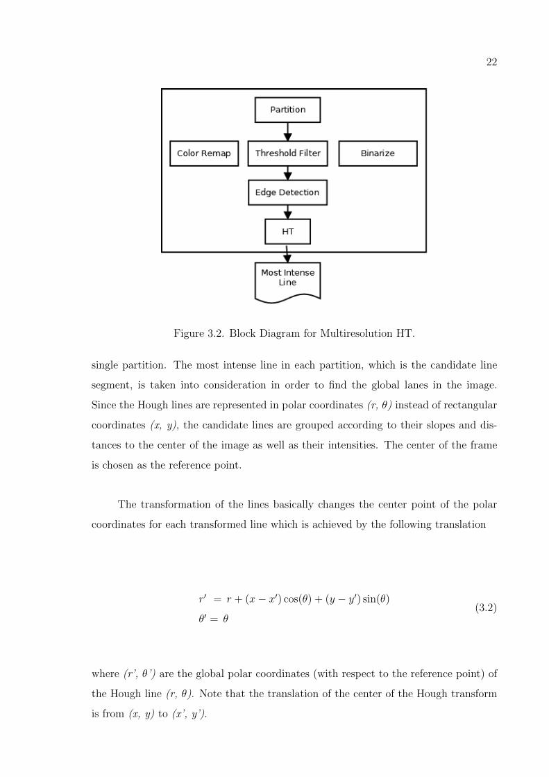
Figure 3.2. Block Diagram for Multiresolution HT.
single partition. The most intense line in each partition, which is the candidate line
segment, is taken into consideration in order to find the global lanes in the image.
Since the Hough lines are represented in polar coordinates (r, θ) instead of rectangular
coordinates (x, y), the candidate lines are grouped according to their slopes and dis-
tances to the center of the image as well as their intensities. The center of the frame
is chosen as the reference point.
The transformation of the lines basically changes the center point of the polar
coordinates for each transformed line which is achieved by the following translation
r′ = r + (x− x′) cos(θ) + (y − y′) sin(θ)
θ′ = θ(3.2)
where (r’, θ’) are the global polar coordinates (with respect to the reference point) of
the Hough line (r, θ). Note that the translation of the center of the Hough transform
is from (x, y) to (x’, y’).

23
Figure 3.3. (a) Partitioned image, (b) Binary image.
Figure 3.4. (a) Candidate lines, (b) Transformed line, (c) Detected lines.
After the lines are grouped, the most intense three clusters are assigned as the
lanes. However, there may be less than three lanes if the sum of the intensities of the
candidate lines is less than a threshold value.
3.1.3. Tracking: HMM
HMM [53] is an alternative to Kalman filter and particle filtering. It is a statistical
model in which the system being modeled is assumed to be a Markov process with
unobserved states. As shown in Figure 3.5, the system consists of predefined sets of
states and observations. A state transition probability matrix defines the probabilities
of transition between states. An emission probability matrix defines the probability of
encountering each observation for each state. System also defines the start probabilities
24
of each state. The ultimate aim of an HMM is to estimate the next observation relying
on the current observation, without access to the state information.
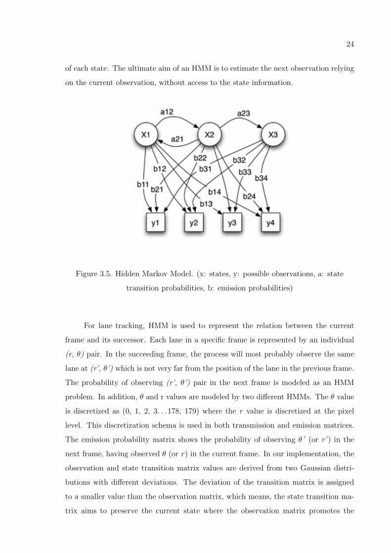
Figure 3.5. Hidden Markov Model. (x: states, y: possible observations, a: state
transition probabilities, b: emission probabilities)
For lane tracking, HMM is used to represent the relation between the current
frame and its successor. Each lane in a specific frame is represented by an individual
(r, θ) pair. In the succeeding frame, the process will most probably observe the same
lane at (r’, θ’) which is not very far from the position of the lane in the previous frame.
The probability of observing (r’, θ’) pair in the next frame is modeled as an HMM
problem. In addition, θ and r values are modeled by two different HMMs. The θ value
is discretized as (0, 1, 2, 3. . . 178, 179) where the r value is discretized at the pixel
level. This discretization schema is used in both transmission and emission matrices.
The emission probability matrix shows the probability of observing θ’ (or r’ ) in the
next frame, having observed θ (or r) in the current frame. In our implementation, the
observation and state transition matrix values are derived from two Gaussian distri-
butions with different deviations. The deviation of the transition matrix is assigned
to a smaller value than the observation matrix, which means, the state transition ma-
trix aims to preserve the current state where the observation matrix promotes the

25
exploration behavior.
3.2. Experiments and Results
The approach proposed in this study is implemented and tested on a relatively
short video sequence of an urban drive. In addition, the proposed approach is compared
with the classical Hough transform where the entire image is processed and the most
intense lines are accepted as candidate lines. The properties of the video are as follows.
Table 3.1. Properties of the video sequence.
Camera Position: Front console of the car
Resolution: 512 x 288
Frame Rate: 29.97
Length: 34 sec.
3.2.1. Setup
As the first step of the experiment, the image is converted to a binary image
using a color remapping function. The mapping for each pixel from 24bit RGB value
to binary value is given in Table 3.2.
Table 3.2. Color remapping.
Pixel Value Red Green Blue
0-175 0 0 0
176-195 1 1 0
196-255 1 1 1
This binarization favors the white and yellow parts of the images. The values
are manually crafted for the sample video. More discussions about improving the color
remapping can be found in the next section.
The next step is to determine the partitions of the image on which the Hough
transforms will be applied. Although the image is 288 pixels high, only the bottommost
116 pixels are used since the road remains in this lower part of the image. The accuracy
of this assumption may slightly differ depending on the slope of the lane.
26
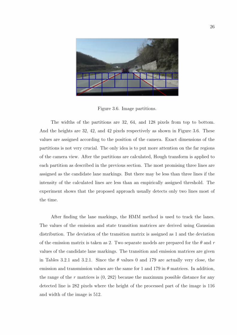
Figure 3.6. Image partitions.
The widths of the partitions are 32, 64, and 128 pixels from top to bottom.
And the heights are 32, 42, and 42 pixels respectively as shown in Figure 3.6. These
values are assigned according to the position of the camera. Exact dimensions of the
partitions is not very crucial. The only idea is to put more attention on the far regions
of the camera view. After the partitions are calculated, Hough transform is applied to
each partition as described in the previous section. The most promising three lines are
assigned as the candidate lane markings. But there may be less than three lines if the
intensity of the calculated lines are less than an empirically assigned threshold. The
experiment shows that the proposed approach usually detects only two lines most of
the time.
After finding the lane markings, the HMM method is used to track the lanes.
The values of the emission and state transition matrices are derived using Gaussian
distribution. The deviation of the transition matrix is assigned as 1 and the deviation
of the emission matrix is taken as 2. Two separate models are prepared for the θ and r
values of the candidate lane markings. The transition and emission matrices are given
in Tables 3.2.1 and 3.2.1. Since the θ values 0 and 179 are actually very close, the
emission and transmission values are the same for 1 and 179 in θ matrices. In addition,
the range of the r matrices is (0, 282) because the maximum possible distance for any
detected line is 282 pixels where the height of the processed part of the image is 116
and width of the image is 512.

27
Table 3.3. (a) Transmission matrix for r, (b) Transmission matrix for θ.
r 0 1 2 3 ... 279 280 281 282
0 0.3989 0.2420 0.0540 0.0044 ... 0.0000 0.0000 0.0000 0.0000
1 0.2420 0.3989 0.2420 0.0540 ... 0.0000 0.0000 0.0000 0.0000
2 0.0540 0.2420 0.3989 0.2420 ... 0.0000 0.0000 0.0000 0.0000
... ... ... ... ... ... ... ... ... ...
280 0.0000 0.0000 0.0000 0.0000 ... 0.2420 0.3989 0.2420 0.0540
281 0.0000 0.0000 0.0000 0.0000 ... 0.0540 0.2420 0.3989 0.2420
282 0.0000 0.0000 0.0000 0.0000 ... 0.0044 0.0540 0.2420 0.3989
θ 0 1 2 3 ... 176 177 178 179
0 0.3989 0.2420 0.0540 0.0044 ... 0.0001 0.0044 0.0540 0.2420
1 0.2420 0.3989 0.2420 0.0540 ... 0.0000 0.0001 0.0044 0.0540
2 0.0540 0.2420 0.3989 0.2420 ... 0.0000 0.0000 0.0001 0.0044
... ... ... ... ... ... ... ... ... ...
177 0.0044 0.0001 0.0000 0.0000 ... 0.2420 0.3989 0.2420 0.0540
178 0.0540 0.0044 0.0001 0.0000 ... 0.0540 0.2420 0.3989 0.2420
179 0.2420 0.0540 0.0044 0.0001 ... 0.0044 0.0540 0.2420 0.3989
3.2.2. Results
The proposed approach managed to detect and track at least one lane in most of
the sequence. In addition, false positives are reduced to an acceptable level. In order
to validate the results, the proposed approach is compared with the classical Hough
Transform approach. In this method, the same part of the image is processed using the
Hough transform routine. The most intensive 10 lines are merged according to their r
and θ values. Finally three or less candidate lines are selected as the lane markings.
The major differences between the classical and the multi-resolution HT are
shown in Figure 3.7. The images on the left hand side are the detected or missed
lines by the classical approach. The right hand side images are the outputs of the new
approach for the same frames which show that the new approach is more robust and
accurate.
The computational cost of the proposed approach can be compared as follows.
The average processing time is 21.25 milliseconds for a laptop PC with Intel T5450
processor at 1.66 GHz whereas the average time of the classical approach is 15.29

28
Table 3.4. (a) Emission matrix for r, (b) Emission matrix for θ.
r 0 1 2 3 4 5 ... 281 282
0 0.1995 0.1760 0.1210 0.0648 0.0270 0.0088 ... 0.0000 0.0000
1 0.1760 0.1995 0.1760 0.1210 0.0648 0.0270 ... 0.0000 0.0000
2 0.1210 0.1760 0.1995 0.1760 0.1210 0.0648 ... 0.0000 0.0000
3 0.0648 0.1210 0.1760 0.1995 0.1760 0.1210 ... 0.0000 0.0000
4 0.0270 0.0648 0.1210 0.1760 0.1995 0.1760 ... 0.0000 0.0000
... ... ... ... ... ... ... ... ... ...
281 0.0000 0.0000 0.0000 0.0000 0.0000 0.0000 ... 0.1995 0.1760
282 0.0000 0.0000 0.0000 0.0000 0.0000 0.0000 ... 0.1760 0.1995
θ 0 1 2 3 4 5 ... 178 179
0 0.1995 0.1760 0.1210 0.0648 0.0270 0.0088 ... 0.1210 0.1760
1 0.1760 0.1995 0.1760 0.1210 0.0648 0.0270 ... 0.0648 0.1210
2 0.1210 0.1760 0.1995 0.1760 0.1210 0.0648 ... 0.0270 0.0648
3 0.0648 0.1210 0.1760 0.1995 0.1760 0.1210 ... 0.0088 0.0270
4 0.0270 0.0648 0.1210 0.1760 0.1995 0.1760 ... 0.0022 0.0088
... ... ... ... ... ... ... ... ... ...
178 0.1210 0.0648 0.0270 0.0088 0.0022 0.0004 ... 0.1995 0.1760
179 0.1760 0.1210 0.0648 0.0270 0.0088 0.0022 ... 0.1760 0.1995
milliseconds.
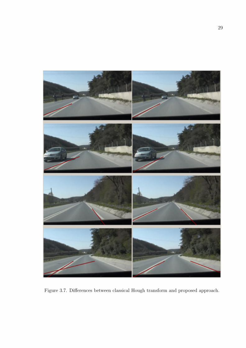
29
Figure 3.7. Differences between classical Hough transform and proposed approach.

30
4. SIGN DETECTION AND TRACKING
There are four types of traffic signs that are used in the traffic code: 1) warning;
2) prohibition; 3) regulatory; and 4) informational. The warning signs are equilateral
triangles with one vertex upwards. They have a white background and are surrounded
by a thick red border. To indicate prohibitions (eg. no parking, no left turn, speed
limits), the signs are circles with white background and red border. Regulatory traffic
signs are intended to instruct road users (not only the drivers) on what they must do
(or not do) under a given set of circumstances. Informative signs have the same color
as the regulatory signs.
Figure 4.1. Traffic signs used in this study.
To detect the position of a sign in the image, we must know the two properties we
discussed previously, i.e., color and shape. Traffic sign detection is more difficult under
adverse lighting and weather conditions despite the fact that road signs are mainly
composed of distinct colors, such as red, blue, black and white. The effect of outdoor
illumination, which varies strictly, cannot be controlled. Thus, the observed color of a
road sign is always a mixture of the original color and whatever the current outdoor
lighting is. Moreover, the paint on signs often deteriorates with age. Thus, a color
model that will cope with these challenges is selected in this study.
There are many possible variations in the appearance of a sign in an image.
Throughout the day, and at night time, lighting conditions can vary enormously. A
sign may be well lit by direct sunlight, or headlights, it may be completely in shadow
on a bright day, or heavy rain may blur the image of the sign. Ideally, signs have
clear color contrast, but over time they can become faded, yet still be clear to drivers.

31
Although the signs mostly appear by the road edge, this may be at a far point from
the car on a multi-lane highway to the left or right, or very close on a single lane track.
Further, while signs are generally a standard distance above the ground, they can also
appear on temporary roadwork signs at ground level. Thus, it is not easy to restrict
the possible positions of a sign within an image of a road scene.
Traffic sign processing proposed in this study consists of two independent phases.
In the first phase 64x64 sized sub-frames are extracted from the video sequence, and in
the second phase these sub-frames are classified according to several learning methods.
This chapter describes the detection process.
4.1. Methodology
The proposed approach for sign detection and tracking in the ADES project
is based on genetic algorithms (GA) [54]. A modified version of radial symmetric
transform [55] is applied after an image binarization step. The lifecycle of a video
frame for the sign detection process is illustrated in Figure 4.2.
Figure 4.2. Sign detection stages. (a) Original frame, (b) Binarized image, (c)
Triangle verified, (d) Sign extracted, (e) Brightness correction applied, (f) Detected
sign.
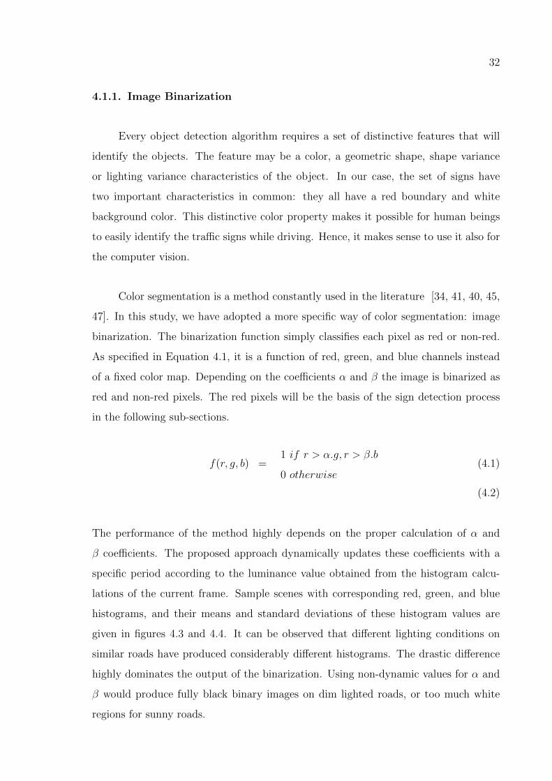
32
4.1.1. Image Binarization
Every object detection algorithm requires a set of distinctive features that will
identify the objects. The feature may be a color, a geometric shape, shape variance
or lighting variance characteristics of the object. In our case, the set of signs have
two important characteristics in common: they all have a red boundary and white
background color. This distinctive color property makes it possible for human beings
to easily identify the traffic signs while driving. Hence, it makes sense to use it also for
the computer vision.
Color segmentation is a method constantly used in the literature [34, 41, 40, 45,
47]. In this study, we have adopted a more specific way of color segmentation: image
binarization. The binarization function simply classifies each pixel as red or non-red.
As specified in Equation 4.1, it is a function of red, green, and blue channels instead
of a fixed color map. Depending on the coefficients α and β the image is binarized as
red and non-red pixels. The red pixels will be the basis of the sign detection process
in the following sub-sections.
f(r, g, b) =1 if r > α.g, r > β.b
0 otherwise(4.1)
(4.2)
The performance of the method highly depends on the proper calculation of α and
β coefficients. The proposed approach dynamically updates these coefficients with a
specific period according to the luminance value obtained from the histogram calcu-
lations of the current frame. Sample scenes with corresponding red, green, and blue
histograms, and their means and standard deviations of these histogram values are
given in figures 4.3 and 4.4. It can be observed that different lighting conditions on
similar roads have produced considerably different histograms. The drastic difference
highly dominates the output of the binarization. Using non-dynamic values for α and
β would produce fully black binary images on dim lighted roads, or too much white
regions for sunny roads.
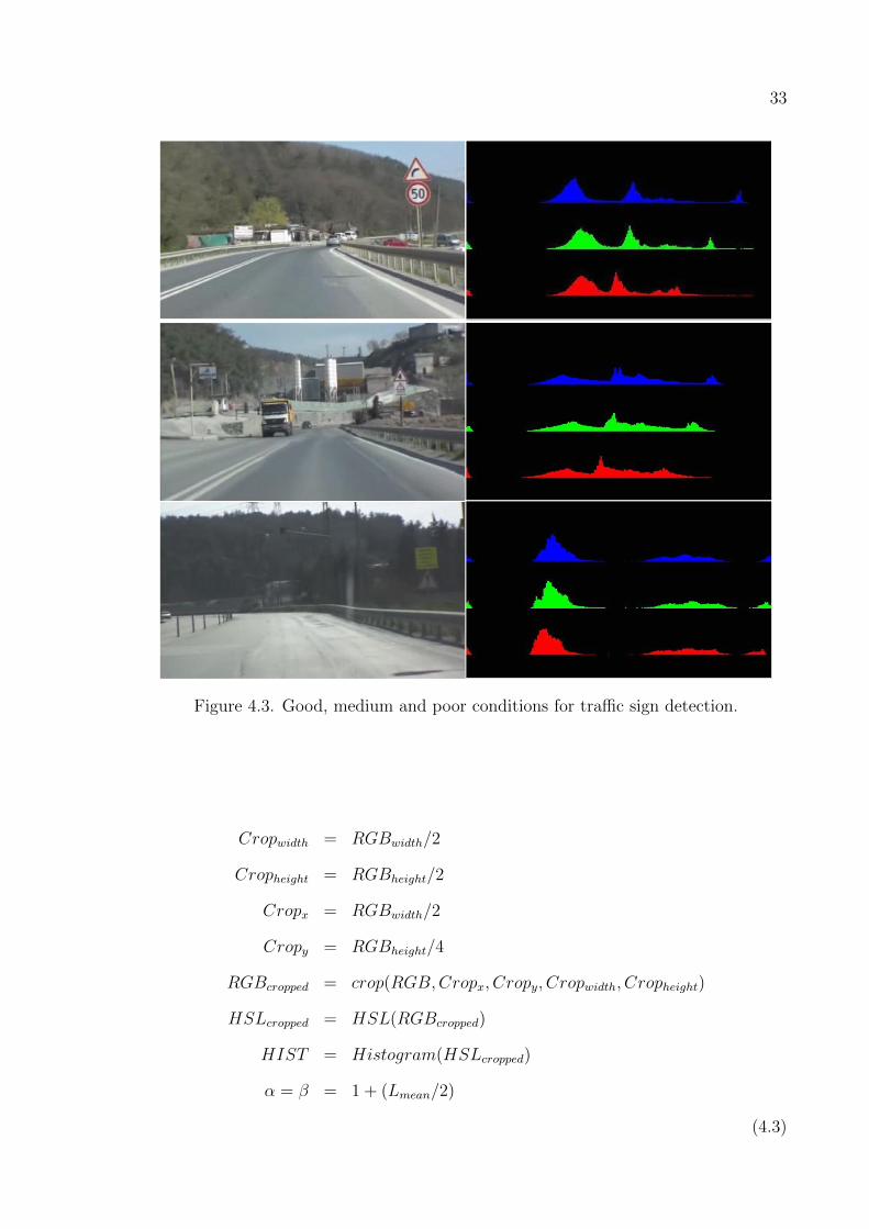
33
Figure 4.3. Good, medium and poor conditions for traffic sign detection.
Cropwidth = RGBwidth/2
Cropheight = RGBheight/2
Cropx = RGBwidth/2
Cropy = RGBheight/4
RGBcropped = crop(RGB,Cropx, Cropy, Cropwidth, Cropheight)
HSLcropped = HSL(RGBcropped)
HIST = Histogram(HSLcropped)
α = β = 1 + (Lmean/2)
(4.3)
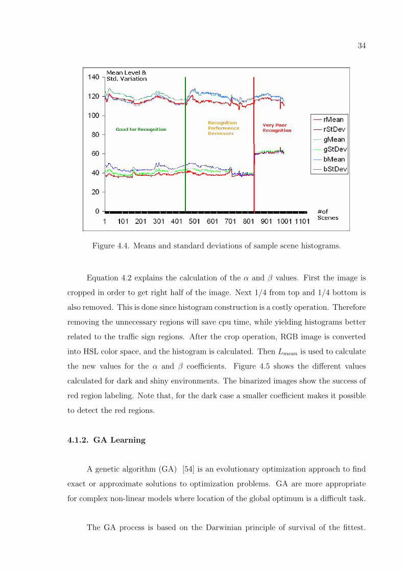
34
Figure 4.4. Means and standard deviations of sample scene histograms.
Equation 4.2 explains the calculation of the α and β values. First the image is
cropped in order to get right half of the image. Next 1/4 from top and 1/4 bottom is
also removed. This is done since histogram construction is a costly operation. Therefore
removing the unnecessary regions will save cpu time, while yielding histograms better
related to the traffic sign regions. After the crop operation, RGB image is converted
into HSL color space, and the histogram is calculated. Then Lmean is used to calculate
the new values for the α and β coefficients. Figure 4.5 shows the different values
calculated for dark and shiny environments. The binarized images show the success of
red region labeling. Note that, for the dark case a smaller coefficient makes it possible
to detect the red regions.
4.1.2. GA Learning
A genetic algorithm (GA) [54] is an evolutionary optimization approach to find
exact or approximate solutions to optimization problems. GA are more appropriate
for complex non-linear models where location of the global optimum is a difficult task.
The GA process is based on the Darwinian principle of survival of the fittest.
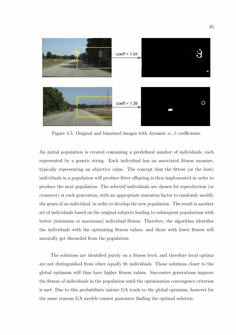
35
Figure 4.5. Original and binarized images with dynamic α, β coefficients.
An initial population is created containing a predefined number of individuals, each
represented by a genetic string. Each individual has an associated fitness measure,
typically representing an objective value. The concept that the fittest (or the best)
individuals in a population will produce fitter offspring is then implemented in order to
produce the next population. The selected individuals are chosen for reproduction (or
crossover) at each generation, with an appropriate mutation factor to randomly modify
the genes of an individual, in order to develop the new population. The result is another
set of individuals based on the original subjects leading to subsequent populations with
better (minimum or maximum) individual fitness. Therefore, the algorithm identifies
the individuals with the optimizing fitness values, and those with lower fitness will
naturally get discarded from the population.
The solutions are identified purely on a fitness level, and therefore local optima
are not distinguished from other equally fit individuals. Those solutions closer to the
global optimum will thus have higher fitness values. Successive generations improve
the fitness of individuals in the population until the optimisation convergence criterion
is met. Due to this probabilistic nature GA tends to the global optimum, however for
the same reasons GA models cannot guarantee finding the optimal solution.
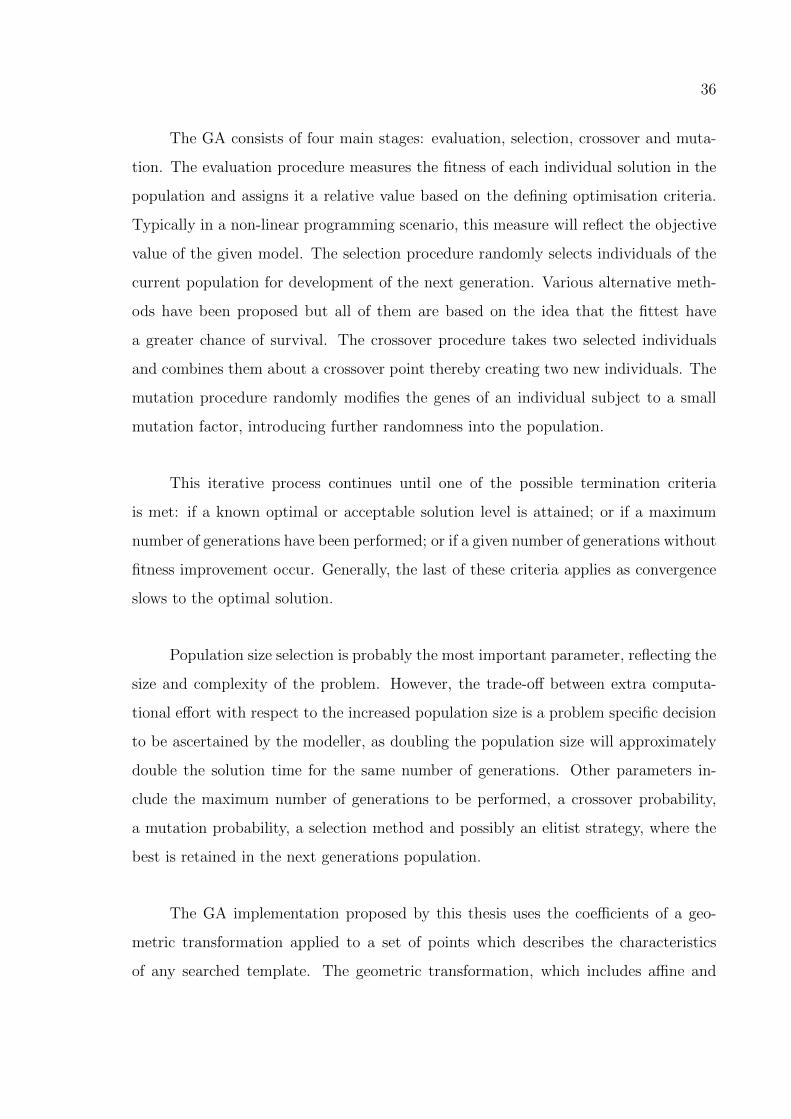
36
The GA consists of four main stages: evaluation, selection, crossover and muta-
tion. The evaluation procedure measures the fitness of each individual solution in the
population and assigns it a relative value based on the defining optimisation criteria.
Typically in a non-linear programming scenario, this measure will reflect the objective
value of the given model. The selection procedure randomly selects individuals of the
current population for development of the next generation. Various alternative meth-
ods have been proposed but all of them are based on the idea that the fittest have
a greater chance of survival. The crossover procedure takes two selected individuals
and combines them about a crossover point thereby creating two new individuals. The
mutation procedure randomly modifies the genes of an individual subject to a small
mutation factor, introducing further randomness into the population.
This iterative process continues until one of the possible termination criteria
is met: if a known optimal or acceptable solution level is attained; or if a maximum
number of generations have been performed; or if a given number of generations without
fitness improvement occur. Generally, the last of these criteria applies as convergence
slows to the optimal solution.
Population size selection is probably the most important parameter, reflecting the
size and complexity of the problem. However, the trade-off between extra computa-
tional effort with respect to the increased population size is a problem specific decision
to be ascertained by the modeller, as doubling the population size will approximately
double the solution time for the same number of generations. Other parameters in-
clude the maximum number of generations to be performed, a crossover probability,
a mutation probability, a selection method and possibly an elitist strategy, where the
best is retained in the next generations population.
The GA implementation proposed by this thesis uses the coefficients of a geo-
metric transformation applied to a set of points which describes the characteristics
of any searched template. The geometric transformation, which includes affine and

37
perspective transformations, is
u′
v′
w
=
a b c
d e f
g h 1
x
y
1
(4.4)
u = u′/w (4.5)
v = v′/w (4.6)
where x and y are the coordinates of the sample point from the template describing
the set of points. u and v are the transformed points on the image. a, b, d, e provide
rotation, scaling and shearing where c and f are used for translation. In addition, g
and h provide perspective transformation in two dimensions. These coefficient values
or a subset of them can be used in the chromosome encoding of the GA.
The effect of the transformation can be visualized better with a simple example.
Assume that a, b, c, d, e, and f coefficients are used in the encoding of the GA
chromosome. In addition, g and h are left zero for simplicity. For this scenario, we can
conclude that a chromosome with the transformation coefficients in Equation 4.6 can
yield the transformed circle and triangular points shown in Figure 4.6. The points on
the left hand side of each figure are the equidistant characteristic points of the circular
and triangular templates, where the points on the right hand sides are the translated,
scaled, and rotated counter parties in the transformed domain.
u
v
1
=
2 1 100
1 2 50
0 0 1
x
y
1
(4.7)
For complex applications, all of the geometric transformation matrix values can
be added to the chromosome encoding in the same manner, however, the resulting
search space may not be convenient for real time applications with limited computa-
tional power. Therefore, in this particular study, only the two translation and one

38
Figure 4.6. Template characteristic points in (x,y) domain, and (u,v) domain after
geometric transformation for circular and triangular signs.
scaling coefficients are included in the chromosome in order to reduce the computa-
tional requirements. The resulting transition matrix is given in Equation 4.7.
u
v
1
=
a 0 c
0 a f
0 0 1
x
y
1
(4.8)
The crossover process is also a function of these coefficients as given in Equation
4.8
anewchromo = αachromo1 + βachromo2
cnewchromo = αcchromo1 + βcchromo2 (4.9)
fnewchromo = αfchromo1 + βfchromo2
1 = α + β
The fitness of the chromosome is evaluated according to the color of the trans-
formed point (u, v) on the binary image. If the value of the pixel is one, which means
it is a red point on the original image, the fitness of the chromosome is increased.
However, this method would yield the highest fitness value for completely red regions.
Therefore another set of template points is introduced in order to indicate the non-red
points on the template. These points are also subject to the transformation. These

39
non-red points are selected inside the region bounded by the red points as shown in
Figure 4.6. In other words, the red points increase the fitness value when they are
white in the binary image, and the black points increase the fitness value when they
are black in the binary image. If the expected color cannot be found, then the fitness
value is decreased for each of the failed points. At each iteration the fitness values
are calculated for each chromosome. At the end of the process the chromosomes are
expected to converge around the traffic sign as shown in Figure 4.7.
Figure 4.7. Initial and converged chromosomes.
After each GA run, half of the converged chromosomes are passed to the next
frame. This provides the tracking of the detected sings in the video stream.
4.1.3. Modified Radial Symmetry
The initial tests have shown that, GA is likely to find non-existing signs in the
regions with relatively high red-color concentration. For preventing false positives, an
additional step of Modified Radial Symmetry check is introduced after the GA.
For circular sign detection, it works as illustrated in Figure 4.8(a). The ”Start”
point is the outcome of the GA. For each candidate point suggested by the GA, the Cir-
cle Validation Algorithm detects the innermost circle that surrounds the point. First,
the algorithm performs a bi-directional horizontal scan, and finds the x-coordinate cen-
ter (Center ]1). The vertical center is detected next, by performing a bi-directional
vertical scan starting from Center ]1. Note that, this is the simplified description of
the algorithm. In the actual implementation, the algorithm employs a probabilistic
approach, and detects the maximum of 2N x 2N candidate circles, where N is the tol-

40
erance coefficient. This coefficient N helps to tolerate the discontinuities on the circle.
Figure 4.8. (a) Circle detection, (b) Scoring of circles.
After the detection step, each candidate circle is scored as displayed in Figure
4.8(b). The scoring function projects the virtual circle onto the binarized image. Next,
a scoring function checks how good the candidate circle overlaps red points in the
binarized image. If the candidate circle really overlaps a circle on the actual image, it
will get a high score. The overlapping check is performed for 36 points (10◦ increment)
in our implementation. Hence the maximum score is 36.
Figure 4.9. Candidate circles, and highest score selection.
Triangular sign validation runs in a slightly different manner. As shown in Figure
4.11(a), the detection phase is similar to that of the circular signs, but scoring is
completely different. The difference in the geometry affects the Center ]2 location,
which is radius/3 upwards from the triangle baseline. Similar to the circular case, the
algorithm detects maximum of 2N x 2N candidate triangles, where N is the tolerance
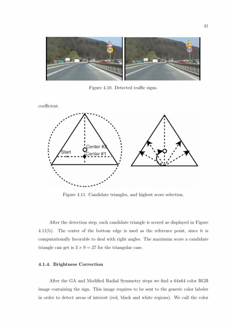
41
Figure 4.10. Detected traffic signs.
coefficient.
Figure 4.11. Candidate triangles, and highest score selection.
After the detection step, each candidate triangle is scored as displayed in Figure
4.11(b). The center of the bottom edge is used as the reference point, since it is
computationally favorable to deal with right angles. The maximum score a candidate
triangle can get is 3 × 9 = 27 for the triangular case.
4.1.4. Brightness Correction
After the GA and Modified Radial Symmetry steps we find a 64x64 color RGB
image containing the sign. This image requires to be sent to the generic color labeler
in order to detect areas of interest (red, black and white regions). We call the color

42
labeler ”Generic” because it can be used to label according to any number of target
colors, as explained in Section 4.1.5. If the target colors are only black and white, it
will simply do binarization.
Figure 4.12. Brightness correction examples.
Similar to the Image Binarization explained in section 4.1.1 the color labeling
is strongly affected by the illumination conditions. In section 4.1.1 we had the full
frame out of which to detect the red and non-red pixels. At this step the condition
is different. We have a 64x64 sized frame which contains a sign with high probability.
Brightness correction is applied directly to this image.
Figure 4.12 shows examples of brightness correction. The procedure uses the
luminance values Lmean already calculated in Equation 4.2. Therefore, does not require
the costly histogram calculations to be executed once again.
4.1.5. Generic Color Labeler
Generic Color Labeler takes an RGB (or HSL) image and an array of target
RGB colors. As explained in Figure 4.1.5 it calculates the distance of each pixel to all
the target RGB colors. The pixels are assigned to colors with the minimal distance.
Calculations for the HSL version are little different as seen in Figure 4.1.5. The value
of each channel is normalized according to scale of 180.
Figure 4.15 illustrates color labeling for black and white target colors. It can
easily be noticed that, labeling in this particular example is done on the basis of only
white and non-white regions. In the earlier stages of the study, labeling was being made

43
Input: 24 bpp RGB color image and an array of target colors
Output: RGB image classified to target colors
foreach pixel Pix do
foreach target color RGBtarget do
Distance = ABS(RGBtarget.R - Pix.R) +
ABS(RGBtarget.G - Pix.G) +
ABS(RGBtarget.B - Pix.B);
end
end
LabelPix = RGBtarget with MinDistance;
Figure 4.13. Generic RGB color labeling algorithm.
for three colors: red, black and white. But as the system evolved, in order to yield
better performance in terms of computation time and output quality, we have adopted
a white and non-white labeling. Note that, this is the second labeling of the image
pixels. The first one, explained in section 4.1.1, was a binarization for detecting red
pixels on image. It was executed on the whole frame rather than a subset of it. This
time, on the other hand, we have a 64x64 sub-frame verified by the GA and the Modified
Radial Symmetry to contain a candidate sign. The subframe is also passed through a
brightness correction step in order to minimize the effect of lighting variations.
4.1.6. Sign Extraction
The aim of the sign extraction step is to exract the meaningful part of the sign
from the circular of triangular frame surrounding it. We first perform a flood fill
operation to convert the black regions around the 64x64 frame. As shown in Figure
4.16, the filling operation starts from the upper left corner of the frame. Next, a sanity
check is performed to verify that the flood fill has only removed the surrounding black
pixels, not the center of the frame. This may happen when all the black pixels are
accidentally connected in the image. Especially, when the lighting conditions are is
poor, the detection step may yield frames with excessive amount of black pixels. After
the flood fill operation we apply a second step of cleaning depending on whether the

44
Input: 24 bpp HSL color image and an array of target colors
Output: HSL image classified to target colors
foreach pixel Pix do
foreach target color HSLtarget do
Distance = ABS((HSLtarget.H - Pix.H) mod 180) +
ABS((HSLtarget.S - Pix.S) x 180) +
ABS((HSLtarget.L - Pix.L) x 180);
end
end
LabelPix = HSLtarget with MinDistance;
Figure 4.14. Generic HSL color labeling algorithm.
Figure 4.15. Color labeling examples (black / white).
sign is circular or triangular. For the circular sigs, a circle of radius 24 is assumed
to contain the interior part of the sign, and anything outside it is cleaned out. For
the triangular case, a triangle as depicted in Figure 4.16 is assumed to surround the
meaningful part of the sign. All pixels outside this virtual triangle are cleaned out.
4.2. Experiments and Results
The experiments are performed with pre-recorded video of 512x288 pixels reso-
lution and 20 fps frame rate. Capturing is done in a car moving with varying speed
in the urban traffic (Appendix A). A wide range of ligthing conditions is included in
the test videos. Sunny roads, dim lighted roads, shadows and even night-time driving
conditions are considered.
The processing is performed on a laptop PC with Intel T5450 processor at 1.66
GHz. Since the sign detection process should be carried out in real time, we tried to
keep the GA population and the number of iterations small. Besides, we used N =2 as

45
Figure 4.16. Extraction of the meaningful part.
Table 4.1. Detection rate of circular signs.
Fitness threshold 30 30 30 35
Population size 60 120 60 60
Epoch number 2 2 4 2
Mutation rate 0.35 0.35 0.35 0.35
Crossover rate 0.75 0.75 0.75 0.75
Selection method Elitist Elitist Elitist Elitist
Milliseconds per frame 9 14 14 9
True positives 95 percent 96 percent 96 percent 65 percent
Misses 5 percent 4 percent 4 percent 35 percent
False positives 5 percent 7 percent 6 percent 1 percent
the tolerance coefficient for the Modified Radial Symmetry step. This lets the second
level of discontinuity in any of the four directions while assuring reasonable processing
time.
It is generally hard to give exact (success and failure) numbers when dealing
with video streams. We have done several measurements and obtained the results in
tables 4.1 and 4.2. The results show almost perfect CPU time requirements. For a
highly acceptable detection process, 9 ms of CPU time is enough. Therefore, it is
possible to re-run the whole process more than hundred times in a second. This gives
an opportunity to utilize the GA to track the detected sign. For this purpose, half of
the best chromosomes at the end of each processed frame are passed to the next frame.

46
Table 4.2. Detection rate of triangular signs.
Fitness threshold 16 16 16 12
Population size 60 150 60 60
Epoch number 2 2 6 2
Mutation rate 0.35 0.35 0.35 0.35
Crossover rate 0.75 0.75 0.75 0.75
Selection method Elitist Elitist Elitist Elitist
Milliseconds per frame 9 16 14 9
True positives 87 percent 88 percent 90 percent 94 percent
Misses 13 percent 12 percent 10 percent 6 percent
False positives 4 percent 4 percent 5 percent 9 percent
The upper parts of the tables 4.1 and 4.2 show the parameter sets, while the lower
parts (painted in gray) show the experiment results. True positives correspond to the
correctly detected signs, whereas the misses are the signs that could not be detected
at all. Sum of true positives and misses is always 100 percent. False positives, on
the other hand, are the cases where the system indicates a sign existence even though
there exists no sign in that location. The first column of values is the preferred set of
parameters for both the circular and the triangular cases.
For the circular signs, a fitness threshold of 30, GA population size of 60 and
epoch number of 2 yields the ideal results in terms of accuracy and CPU time. It is
possible to enhance the accuracy to 96 percent by increasing either the population size
or the epoch number. But this will almost double the processing time for a very small
accuracy enhancement, hence not worth the trade-off. Fitness threshold, on the other
hand, has considerable effect on the accuracy, as seen on the rightmost column.
The triangular sign process yields the ideal results with a fitness threshold of 16.
That is due to the different geometric characteristics of the triangular signs. The true
positives rate degrades from 95 percent to 87 percent. It is possible to increase this
value by decreasing the fitness threshold from 16 to 12. But this has a side-effect of
increasing the false positives from 4 percent to 9 percent.

47
5. SIGN CLASSIFICATION
5.1. Methodology
The sign detection process explained in the previous section finds 64x64 binary
images that contain the interior part of the traffic signs isolated from the red borders
(see Fig. 5.4). These are human readable images but still need to be classified and
mapped into the predefined set of signs listed in Figure 4.1. In the computer science
literature neural networks (NN), support vector machines (SVM), k-nearest neighbor
and AdaBoost are among the commonly used classifying methods. Our study has
employed the NN and SVM for sign classification.
The training of NN and SVM is done by using various features. Two types of
feature extraction schemes have been employed (see Sections 5.1.2 and 5.1.3). The first
one is a Center of Mass (CoM) dependent occupancy grid matrix implementation,
whereas the second one is based on SURF features [56] of magnified images. Both
methods are highly dependent on the center of mass of the detected image. The
necessity of using CoM is explained in the following section.
5.1.1. Center of Mass (CoM)
Sign detection (Chapter 4) will not always yield perfect outputs. As shown in
Figure 5.1, the detection output may not be always centered. In majority of the cases
the CoM (identified by blue) will not overlap the center of the 64x64 image (identified by
red color). Therefore we calculate the CoM of the detected sign and use this information
for both of the feature exraction schemes as explained in the corresponding sections.
The general idea about using CoM is to crop a smaller region of interest around the
CoM. SURF and occupancy grid will execute on the cropped region.
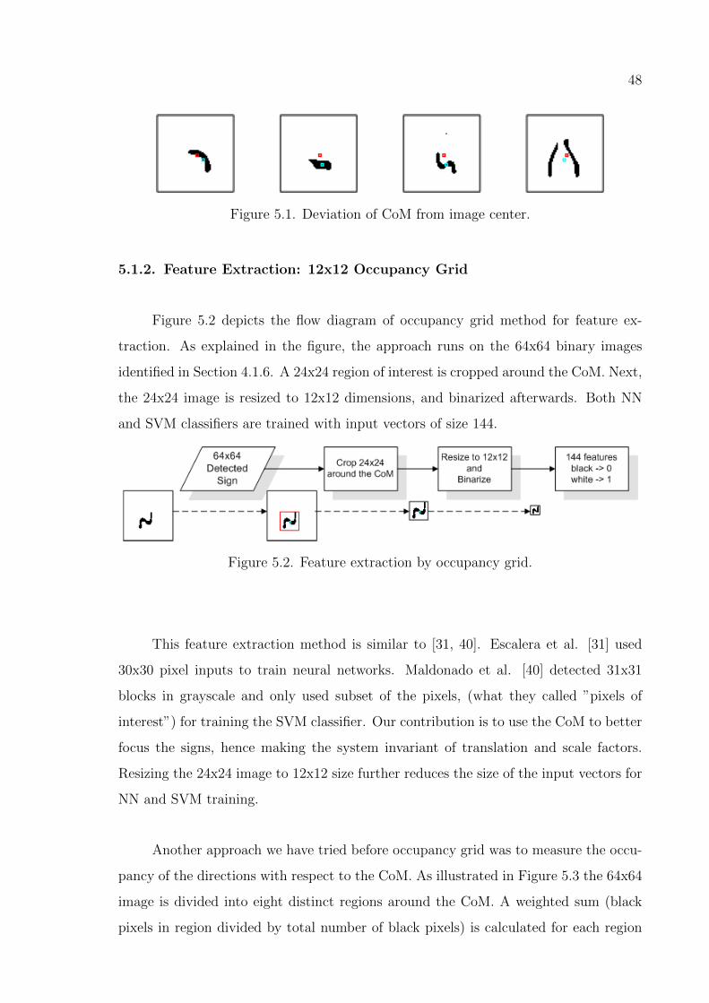
48
Figure 5.1. Deviation of CoM from image center.
5.1.2. Feature Extraction: 12x12 Occupancy Grid
Figure 5.2 depicts the flow diagram of occupancy grid method for feature ex-
traction. As explained in the figure, the approach runs on the 64x64 binary images
identified in Section 4.1.6. A 24x24 region of interest is cropped around the CoM. Next,
the 24x24 image is resized to 12x12 dimensions, and binarized afterwards. Both NN
and SVM classifiers are trained with input vectors of size 144.
Figure 5.2. Feature extraction by occupancy grid.
This feature extraction method is similar to [31, 40]. Escalera et al. [31] used
30x30 pixel inputs to train neural networks. Maldonado et al. [40] detected 31x31
blocks in grayscale and only used subset of the pixels, (what they called ”pixels of
interest”) for training the SVM classifier. Our contribution is to use the CoM to better
focus the signs, hence making the system invariant of translation and scale factors.
Resizing the 24x24 image to 12x12 size further reduces the size of the input vectors for
NN and SVM training.
Another approach we have tried before occupancy grid was to measure the occu-
pancy of the directions with respect to the CoM. As illustrated in Figure 5.3 the 64x64
image is divided into eight distinct regions around the CoM. A weighted sum (black
pixels in region divided by total number of black pixels) is calculated for each region

49
and NN or SVM classifier was trained with input vectors of length eight. The method
was dropped because the desired level of convergence could not be reached. The main
problem here was that, the pixels in close proximity of the CoM are more decisive. But
the method does not distinguish between the near and far pixels. The only considera-
tion is the angle θ with respect to the CoM. Missing the proximity information leads
the method to fail.
Figure 5.3. Feature extraction in polar coordinates.
5.1.3. Feature Extraction: SURF Interest Points
SURF is a scale and rotation invariant feature detector approach. It is basically
derived from SIFT [57] but outperforms in terms of speed, robustness and distinctive-
ness. SURF has several parameters that may affect its output:
• Upright: This parameter determines whether to run Upright SURF (U-SURF) or
not. U-SURF better fits the horizontal camera cases. It runs invariant of image
rotation and therefore consumes less CPU time.
• Octaves: The scale space is divided into number of octaves. The filter size is
affected by the octave levels.
• Intervals: This is the sampling interval. Together with the number of octaves, it
determines the number of filters to be applied. (Number of filters = octaves x
intervals)
• Threshold: A threshold value to control the accuracy of the results. Increasing
the threshold value will decrease the number of detected interest points.

50
Figure 5.4 displays the effect of parameter changes on the output. The SURF in-
terest points are displayed with circles. Each interest point has the following associated
with it:
• (x, y): The center of the SURF interest point.
• Orientation: This is the orientation of the detected feature in radians. In the
U-SURF case it is always zero.
• Scale: The number of octaves decides the cardinality of the state space. Therefore
scale takes values from 1 up to the number of octaves.
• Laplacian: Value is either 1 or -1. This is the sign (positive or negative indicator)
of the Laplacian for the interest point. A value of 1 indicates bright blobs on
dark backgrounds, and -1 indicates just the reverse situation.
Figure 5.4. Parameter effects on SURF output.
The principal idea displayed in Figure 5.4 is the difference between ordinary
SURF and the U-SURF. It is evident that U-SURF does not include any orientation
info. Another important thing is that, sometimes it may be necessay to play with the
parameters for finding the interest points. For example, the first set of parameters have

51
not succeded to find any interest point in the very first sign. Changing the octave and
interval parameters also did not help. But reducing the threshold value from 0.001 to
0.0001 has led to an interest point in the image. The same situation is also valid for
the U-SURF case.
The second thing we can notice is that, ordinary SURF and the U-SURF find
exactly the same interest points with the same scale and Laplacian values. This is
because of the horizotal camera usage. Based on this observation, this study uses the
U-SURF approach throughout the experiments.
Finally, it can be stated that the SURF parameters may not always lead to
interest points. Therefore the system may need to run SURF several times by changing
the parameters. The interest points found by each run must be consolidated until a
maximum number of features or maximum number of iterations is reached.
Figure 5.5. U-SURF results for different sign types (octaves=3, intervals=5).
Figure 5.5 shows the U-SURF results for different sign types. In most of the
cases it seems distinctive enough. But notice the shadowed signs in Figure 5.5. The
SURF features other than the y-coordinate are the same for completely different signs.
Therefore we cannot directly rely on the x or y-coordinate values because the detection
step may not be able to center the sign in 64x64 frame. Another observation is that,
the system will require several interest points to distinguish the signs clearly. The

52
absolute position of the interest points has no significance, but the relative positions
with respect to each other or the CoM is important.
Figure 5.6. Misplacement due to detection step may lead to ambiguities.
Figure 5.6 more clearly illustrates the ambiguities that may occur due to misplace-
ment of the detected figure. If the detection step causes some translation in the vertical
or the horizontal axis, the (x, y) values of the SURF features may become the same
for completely different sign figures. This particular example clearly demonstrates the
necessity of CoM usage to help the U-SURF algorithm perform better. Misplacement
will not affect the orientation, scale and the laplacian of the SURF interest points, but
(x, y) coordinates will become completely unreliable.
We have tried several approaches to overcome this problem. In the early stages of
the study, we have proposed a transformation of interest points from (x, y) coordinate
system into (r, θ) polar coordinates. CoM would be the origin of the target coordinate
system. Each interest point (x, y) was represented by an (r, θ) pair with respect to
the CoM. We transformed the SURF interest points according to equation 5.1. The
method was abandoned because the NN trained with these features did not converge.

53
xdiff = x− CoMx
ydiff = y − CoMy
r =√
(xdiff )2 + (ydiff )2 (5.1)
θ =
arctan(ydiff/xdiff ) if xdiff > 0, ydiff ≥ 0
π − arctan(−ydiff/xdiff ) if xdiff < 0, ydiff ≥ 0
π + arctan(ydiff/xdiff ) if xdiff < 0, ydiff < 0
(2 × π) − arctan(−ydiff/xdiff ) if xdiff > 0, ydiff < 0
Another attempt was to use the (x, y) values of the SURF interest points together
with the corresponding scale factors. This approach also did not converge for NN
training. The main problem with this method and the previos one is that, the input
vectors were interest point oriented. For each interest point detected, two values (r
and θ) were added in the first approach, or three values (x, y, scale) were added in
the second approach. But the number of interest points is completely unpredictable
and varies from sign to sign (64x64 images in our case). On the other hand, NN and
SVM training requires fixed-size input vectors. In order to fit the fixed size, we either
eliminated some of the iterest points (when too many of them are detected) or used
some interest points several times (when too few of them are detected).
Therefore it is evident that we should devise a scheme that has a fixed size for
all detected signs. The final decision about SURF interest points is to group them
according to their position relative to the CoM. This method has proved to perform
well in our experiments. The essentials of our SURF methodology can be listed as:
• Get rid of the unnecessary white regions sorrounding the figure,
• Magnify the image to 128x128 to find as many SURF interest points as possible,
• Binarize magnified image and re-locate the CoM,
• Apply U-SURF and only use the interest points that correspond to the black
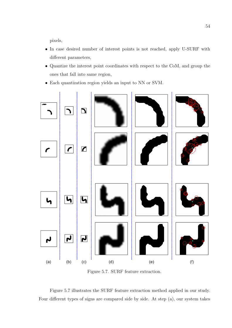
54
pixels,
• In case desired number of interest points is not reached, apply U-SURF with
different parameters,
• Quantize the interest point coordinates with respect to the CoM, and group the
ones that fall into same region,
• Each quantization region yields an input to NN or SVM.
Figure 5.7. SURF feature extraction.
Figure 5.7 illustrates the SURF feature extraction method applied in our study.
Four different types of signs are compared side by side. At step (a), our system takes

55
the 64x64 images from the sign detector. The CoM is calculated for these figures. At
step (b), the images are cropped to 33x33 sub-frames around the CoM (16 pixels to
each direction). Next, another crop operation is perfomed, at step (c), to get rid of the
unnecessary white regions around the sign figure. To do this, 33x33 image is scanned to
find the minimum/maximum coordinates of black pixels (leftmost, rightmost, topmost
and bottommost). The crop size is not fixed but rather depends on the extent of the
black figure in the frame. Having two steps of crop operation is necessary because 64x64
images may contain some noise. For instance, the first image of Figure 5.7 contains a
noisy region. The first step of crop operation gets rid of the noise, and the second step
will clean the unnecessary white surroundings.
The cropped image is magnified to size 128x128 at step (d). The reason for
this is that, SURF can generate much more interest points for larger scale images.
This deduction is reached after several executions of SURF algorithm on smaller scale
images. For 64x64 images, SURF is observed to generate 0 to 10 interest points. For
32x32 images it is observed to generate 0 to 4 interest points. For 128x128 images, on
the other hand, SURF generates 10 to 60 interest points. Since we will be using only
the ones corresponding to black pixels, this amount of interest points barely suffices.
The magnified images are not binary any more. Therefore a binarization is performed
as shown in step (e). Finally, U-SURF is executed and interest points are obtained. As
you can see in (f), the system ignores interest points corresponding to white regions.
Only black region interest points are considered for training.
Figure 5.8 shows how the detected interest points are quantized around the CoM.
The 128x128 image is divided into 12x12 segments. Notice that the segment containing
the CoM is indexed as zero. A total of 9x9=81 equally-sized segments is created. The
size of the segments is parametric, but we fixed it to 12 after testing values from 8 to
14. The maximum number it can be is 14 because 9x14=126 is just 2 pixels smaller
than the magnified image extent, which is 128. For each segment a weighted sum is
computed to be:
Wregion = Countinterest points in region/Counttotal number interest points
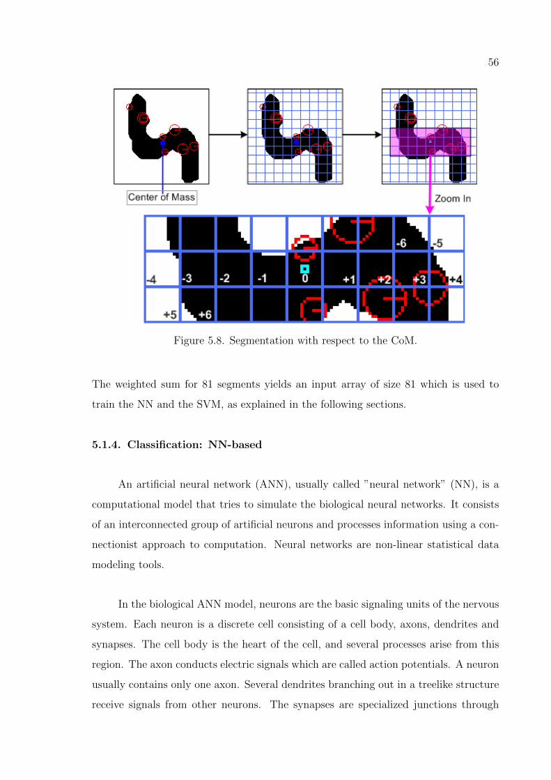
56
Figure 5.8. Segmentation with respect to the CoM.
The weighted sum for 81 segments yields an input array of size 81 which is used to
train the NN and the SVM, as explained in the following sections.
5.1.4. Classification: NN-based
An artificial neural network (ANN), usually called ”neural network” (NN), is a
computational model that tries to simulate the biological neural networks. It consists
of an interconnected group of artificial neurons and processes information using a con-
nectionist approach to computation. Neural networks are non-linear statistical data
modeling tools.
In the biological ANN model, neurons are the basic signaling units of the nervous
system. Each neuron is a discrete cell consisting of a cell body, axons, dendrites and
synapses. The cell body is the heart of the cell, and several processes arise from this
region. The axon conducts electric signals which are called action potentials. A neuron
usually contains only one axon. Several dendrites branching out in a treelike structure
receive signals from other neurons. The synapses are specialized junctions through

57
which neurons signal to each other and to non-neuronal cells, such as muscles.
In the computational ANN model, the synapses of the neuron are modeled as
weights. The strength of the connection between an input and a neuron is noted
by the value of the weight. Negative weight values reflect inhibitory connections,
while positive values designate excitatory connections. Finally, an activation function
controls the amplitude of the output of the neuron. An acceptable range of output is
usually between 0 and 1, or -1 and 1. In most cases the ANN is an adaptive system
that changes its structure based on external or internal information that flows through
the network during the learning phase. The learning procedure tries to find a set of
connections (or weights) w that gives a mapping that fits the training set well.
Furthermore, neural networks can be viewed as highly non-linear functions with
the basic form:
F (x,w) = y
where x is the input vector presented to the network, w are the weights of the network,
and y is the corresponding output vector approximated or predicted by the network.
This view of network as a parameterized function will be the basis for applying standard
function optimization methods to solve the problem of neural network training. Various
Figure 5.9. a) Biological neurons, b) Artificial neural networks.
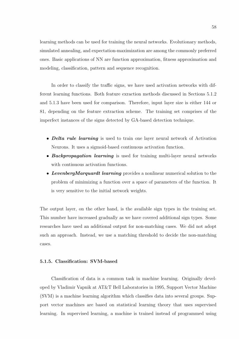
58
learning methods can be used for training the neural networks. Evolutionary methods,
simulated annealing, and expectation-maximization are among the commonly preferred
ones. Basic applications of NN are function approximation, fitness approximation and
modeling, classification, pattern and sequence recognition.
In order to classify the traffic signs, we have used activation networks with dif-
ferent learning functions. Both feature exraction methods discussed in Sections 5.1.2
and 5.1.3 have been used for comparison. Therefore, input layer size is either 144 or
81, depending on the feature extraction scheme. The training set comprises of the
imperfect instances of the signs detected by GA-based detection technique.
• Delta rule learning is used to train one layer neural network of Activation
Neurons. It uses a sigmoid-based continuous activation function.
• Backpropagation learning is used for training multi-layer neural networks
with continuous activation functions.
• LevenbergMarquardt learning provides a nonlinear numerical solution to the
problem of minimizing a function over a space of parameters of the function. It
is very sensitive to the initial network weights.
The output layer, on the other hand, is the available sign types in the training set.
This number have increased gradually as we have covered additional sign types. Some
researches have used an additional output for non-matching cases. We did not adopt
such an approach. Instead, we use a matching threshold to decide the non-matching
cases.
5.1.5. Classification: SVM-based
Classification of data is a common task in machine learning. Originally devel-
oped by Vladimir Vapnik at AT&T Bell Laboratories in 1995, Support Vector Machine
(SVM) is a machine learning algorithm which classifies data into several groups. Sup-
port vector machines are based on statistical learning theory that uses supervised
learning. In supervised learning, a machine is trained instead of programmed using
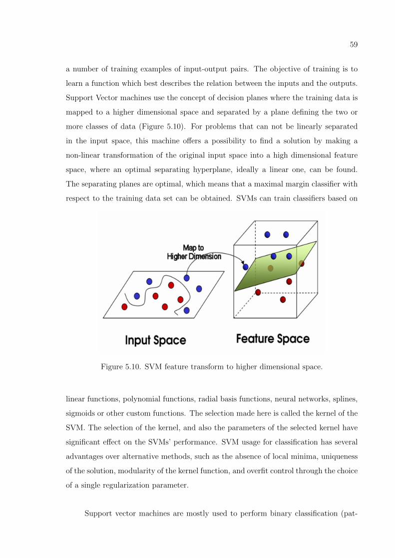
59
a number of training examples of input-output pairs. The objective of training is to
learn a function which best describes the relation between the inputs and the outputs.
Support Vector machines use the concept of decision planes where the training data is
mapped to a higher dimensional space and separated by a plane defining the two or
more classes of data (Figure 5.10). For problems that can not be linearly separated
in the input space, this machine offers a possibility to find a solution by making a
non-linear transformation of the original input space into a high dimensional feature
space, where an optimal separating hyperplane, ideally a linear one, can be found.
The separating planes are optimal, which means that a maximal margin classifier with
respect to the training data set can be obtained. SVMs can train classifiers based on
Figure 5.10. SVM feature transform to higher dimensional space.
linear functions, polynomial functions, radial basis functions, neural networks, splines,
sigmoids or other custom functions. The selection made here is called the kernel of the
SVM. The selection of the kernel, and also the parameters of the selected kernel have
significant effect on the SVMs’ performance. SVM usage for classification has several
advantages over alternative methods, such as the absence of local minima, uniqueness
of the solution, modularity of the kernel function, and overfit control through the choice
of a single regularization parameter.
Support vector machines are mostly used to perform binary classification (pat-
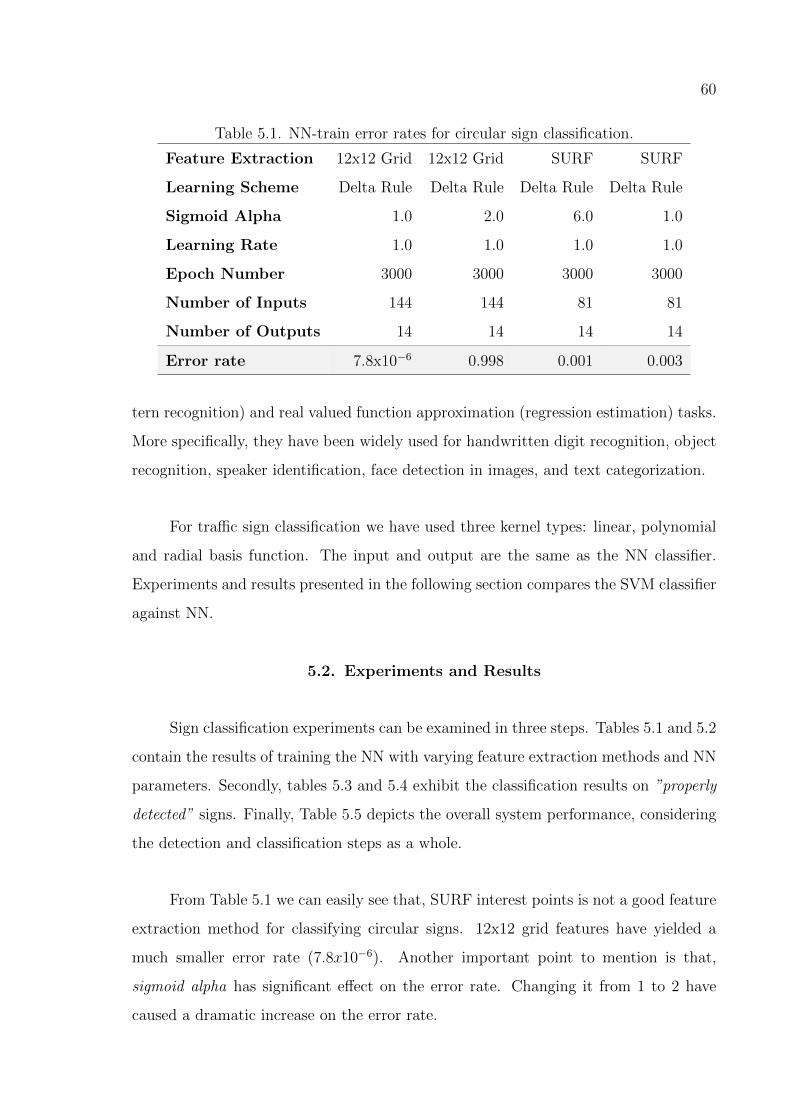
60
Table 5.1. NN-train error rates for circular sign classification.
Feature Extraction 12x12 Grid 12x12 Grid SURF SURF
Learning Scheme Delta Rule Delta Rule Delta Rule Delta Rule
Sigmoid Alpha 1.0 2.0 6.0 1.0
Learning Rate 1.0 1.0 1.0 1.0
Epoch Number 3000 3000 3000 3000
Number of Inputs 144 144 81 81
Number of Outputs 14 14 14 14
Error rate 7.8x10⁻⁶ 0.998 0.001 0.003
tern recognition) and real valued function approximation (regression estimation) tasks.
More specifically, they have been widely used for handwritten digit recognition, object
recognition, speaker identification, face detection in images, and text categorization.
For traffic sign classification we have used three kernel types: linear, polynomial
and radial basis function. The input and output are the same as the NN classifier.
Experiments and results presented in the following section compares the SVM classifier
against NN.
5.2. Experiments and Results
Sign classification experiments can be examined in three steps. Tables 5.1 and 5.2
contain the results of training the NN with varying feature extraction methods and NN
parameters. Secondly, tables 5.3 and 5.4 exhibit the classification results on ”properly
detected” signs. Finally, Table 5.5 depicts the overall system performance, considering
the detection and classification steps as a whole.
From Table 5.1 we can easily see that, SURF interest points is not a good feature
extraction method for classifying circular signs. 12x12 grid features have yielded a
much smaller error rate (7.8x10⁻⁶). Another important point to mention is that,
sigmoid alpha has significant effect on the error rate. Changing it from 1 to 2 have
caused a dramatic increase on the error rate.

61
Table 5.2. NN-train error rates for triangular sign classification.
Feature Extraction 12x12 Grid 12x12 Grid SURF SURF
Learning Scheme Delta Rule Delta Rule Delta Rule Delta Rule
Sigmoid Alpha 1.0 3.0 6.0 3.0
Learning Rate 1.0 1.0 1.0 1.0
Epoch Number 3000 3000 3000 3000
Number of Inputs 144 144 81 81
Number of Outputs 14 14 14 14
Error rate 2.2x10⁻⁶ 0.5 1.7x10⁻⁶ 7.3x10⁻⁶
Table 5.3. Classification success rate of circular signs.
Classification Method NN NN SVM SVM
Feature Extraction 12x12 Grid SURF 12x12 Grid SURF
Milliseconds per frame 5 115 10 120
Error rate 9 percent 18 percent 20 percent 25 percent
On the other hand, Table 5.2 indicates good results for SURF interest points.
Most favorable error rate (1.7x10⁻⁶) have been reached when SURF interest points
are trained with a sigmoid alpha of 6. Again, the influence of sigmoid alpha is worth
mentioning.
Table 5.3 compares the NN classifier against the SVM classifier. As mentioned
before, this table only considers the classification rate of the ”properly detected” signs.
NN subject to this table is an activation network with Delta Rule Learning, while
subject SVM uses a three degrees polynomial kernel. Both classifiers are trained with
12x12 grid and SURF feature extraction methods. NN classifier trained with 12x12
grid have outperformed in terms of both speed and error rate. Besides, SURF features
usage does not seem convenient for circular sign classification.
Table 5.4 gives the classification results for triangular signs. This time SURF re-
sults are acceptable. But SURF apparently consumes much more CPU time compared
to the 12x12 grid method.

62
Table 5.4. Classification success rate of triangular signs.
Classification Method NN NN SVM SVM
Feature Extraction 12x12 Grid SURF 12x12 Grid SURF
Milliseconds per frame 3 113 6 125
Error rate 7 percent 7 percent 9 percent 15 percent
Table 5.5. Overall system performance.
CIRCULAR
Classification Method NN SVM
Feature Extraction 12x12 Grid SURF 12x12 Grid SURF
Milliseconds per frame 14 124 19 129
Error rate 14 percent 22 percent 24 percent 29 percent
TRIANGULAR
Classification Method NN SVM
Feature Extraction 12x12 Grid SURF 12x12 Grid SURF
Milliseconds per frame 12 122 15 134
Error rate 11 percent 11 percent 13 percent 19 percent
Overall system performance shown in Table 5.5 basically consolidates the detec-
tion and classification phases. The errors of detection step are penetrated into the
classification process. For both circular and triangular signs, NN with 12x12 grid fea-
tures have yielded the best results in terms of CPU time and error rate. Triangular
sign detection is more successful. This is due to the sign extraction step explained in
Figures 5.2 and 5.7. While retrieving the central part of the traffic sign, a diameter
of 33 pixels suffices for triangular signs. But circular signs require 51 pixels diameter.
Therefore the exracted sign has less magnification for circular signs, which causes loss
of detail.
63
6. CONCLUSIONS
Lane tracking is one of the major tasks in autonomous urban driving. This thesis
has proposed a MHT-HMM hybrid solution to the problem. The performance of the
resulting system is increased. However there are certain assumptions and shortcomings
of the proposed approach. First of all, variable lighting and road conditions require
adaptive color remapping. Although this is beyond the scope of this work, it is crucial
for a final product. In addition, the proposed approach models the lane boundaries as
lines, therefore an approximation is inevitable at curves. However, it is also possible
to use combination of line segments which are detected at each image partition. As
another future work, the emission matrix can be updated on-the-fly by already made
decisions.
The thesis has also proposed a GA approach for the traffic sign detection problem.
The novel contribution is the injection of geometric transformation matrix into GA.
This makes the system immune to the rotated and translated signs. Another contri-
bution is the radial symmetry check for the GA output. This additional step provides
the better generations to cross over. It acts like a sanity check for the fitness function
and forms the basis for preventing false positives. Although only circular and triangu-
lar signs are described in this study, the existing implementation can also process any
kind of sign which can be described by a set of characteristic points. A success rate
of 95 percent in 9 milliseconds processing time proves the method to be applicable in
real-time applications.
The proposed detection method has certain shortcomings. First of all the image
binarization process may suffer from poor lighting conditions and may require addi-
tional adaptation processes for special conditions like driving at night time and bad
weather conditions. An adaptive brightness correction method is introduced which can
handle most of the cases. But still needs further enhancements, especially for environ-
ments with too much red color. As a future work, injecting more semantic rules into
the system may help. This will let the system distinguish the sign candidate regions

64
from the road, vehicles, sky and buildings in advance. In this way, brightness correction
will only be made for candidate regions, thus helping to further reduce the error rate.
NN and SVM classifiers have been used for sign recognition. Two different meth-
ods have been used for feature extraction: 12x12 Occupancy Grid and U-SURF interest
points. Occupancy grid method apparently outperforms in terms of execution time.
It is ten to twenty times faster than U-SURF. Regarding the error rates, U-SURF
performs better just for the triangular signs.
The performance of the overall system is highly influenced by the sign extraction
step performed right after the detection process. This step aims to isolate the central
part of the traffic sign. Misplacements in the detected sign generally complicates the
isolation operation. The errors in the isolated image are propagated to the classifying
process.

65
APPENDIX A: VIDEO CAPTURING SYSTEM
Figure A.1. The video camera mounted on the car console.
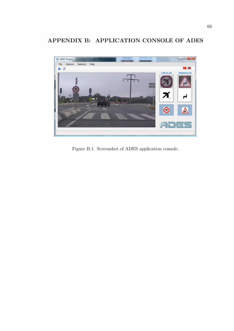
66
APPENDIX B: APPLICATION CONSOLE OF ADES
Figure B.1. Screenshot of ADES application console.

67
APPENDIX C: WARNING SIGNS IN TURKEY
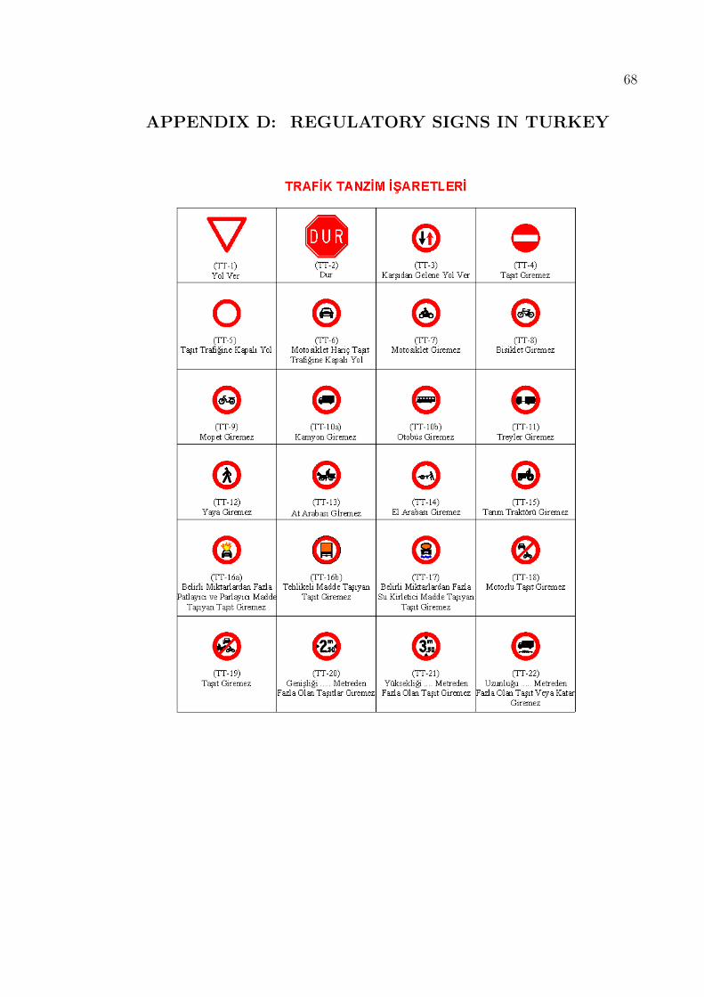
68
APPENDIX D: REGULATORY SIGNS IN TURKEY

69
APPENDIX E: PROHIBITION SIGNS IN TURKEY

70
APPENDIX F: INFORMATIONAL SIGNS IN TURKEY

71
REFERENCES
1. R. Manduchi, A. Castano, A. Talukder, and L. Matthies. Obstacle detection and
terrain classification for autonomous off-road navigation. Auton. Robots, 18(1):81–
102, 2005.
2. U. Franke, D. Gavrila, S. Gorzig, F. Lindner, F. Puetzold, and C. Wohler. Au-
tonomous driving goes downtown. Intelligent Systems and their Applications,
IEEE, 13(6):40–48, Nov/Dec 1998.
3. Darpa grand challenge. http://www.darpa.mil/grandchallenge, 2004-2007.
4. Continental advanced driver assistance systems. http://www.conti-
online.com/generator/www/de/en/continental/automotive/ themes/ com-
mercial vehicles/adas/index en.html.
5. Mercedes benz speed limit assist. http://www.emercedesbenz.com/Nov08/
12 001505 Mercedes Benz TecDay Special Feature Lane Keeping Assist And Speed
Limit Assist.html.
6. European commission: European transport policy for 2010.
http://europa.eu/legislation summaries/environment/tackling climate
change/l24007 en.htm, Oct 2007.
7. P.V. Hough. Method and means for recognizing complex patterns, 1962.
8. James A Anderson. An introduction to neural networks. The MIT Press, 1997.
9. Richard Bellman. Some problems in the theory of dynamic programming. Econo-
metrica, 22(1):37–48, 1954.
10. A.K. Jain, Yu Zhong, and S. Lakshmanan. Object matching using deformable
templates. Pattern Analysis and Machine Intelligence, IEEE Transactions on,

72
18(3):267–278, Mar 1996.
11. Greg Welch and Gary Bishop. An introduction to the kalman filter. Technical
report, Chapel Hill, NC, USA, 1995.
12. Qing Li, Nanning Zheng, and Hong Cheng. Springrobot: a prototype autonomous
vehicle and its algorithms for lane detection. Intelligent Transportation Systems,
IEEE Transactions on, 5(4):300–308, Dec. 2004.
13. B. Yu and A.K. Jain. Lane boundary detection using a multiresolution hough
transform. In Image Processing, 1997. Proceedings., International Conference on,
volume 2, pages 748–751 vol.2, Oct 1997.
14. J.C. McCall and M.M. Trivedi. Video-based lane estimation and tracking for driver
assistance: survey, system, and evaluation. Intelligent Transportation Systems,
IEEE Transactions on, 7(1):20–37, March 2006.
15. W.T. Freeman and E.H. Adelson. The design and use of steerable filters. Pat-
tern Analysis and Machine Intelligence, IEEE Transactions on, 13(9):891–906,
Sep 1991.
16. Dean Pomerleau. Neural network vision for robot driving. In M. Arbib, editor,
The Handbook of Brain Theory and Neural Networks. 1995.
17. Dong-Joong Kang and Mun-Ho Jung. Road lane segmentation using dynamic
programming for active safety vehicles. Pattern Recogn. Lett., 24(16):3177–3185,
2003.
18. Yue Wang, Eam Khwang Teoh, and Dinggang Shen. Lane detection using b-snake.
Information, Intelligence, and Systems, International Conference on, 0:438, 1999.
19. Michael Kass, Andrew Witkin, and Demetri Terzopoulos. Snakes: Active contour
models. INTERNATIONAL JOURNAL OF COMPUTER VISION, 1(4):321–331,
1988.

73
20. K. Kluge and S. Lakshmanan. A deformable-template approach to lane detection.
In Intelligent Vehicles ’95 Symposium., Proceedings of the, pages 54–59, Sep 1995.
21. Heikki Haario, Eero Saksman, and Johanna Tamminen. An adaptive metropolis
algorithm. Bernoulli, 7:223–242, 2001.
22. C. Kreucher, S. Lakshmanan, and K. Kluge. A driver warning system based on the
lois lane detection algorithm. In Proceedings of IEEE International Conference on
Intelligent Vehicles, pages 17–22. Stuttgart, Germany, 1998.
23. S. Lakshmanan and K. Kluge. Lois: A real-time lane detection algorithm. In In
Proceedings of the 30th Annual Conference on Information Sciences and Systems,
1996.
24. N. Apostoloff and A. Zelinsky. Robust vision based lane tracking using multiple
cues and particle filtering. In Intelligent Vehicles Symposium, 2003. Proceedings.
IEEE, pages 558–563, June 2003.
25. Y. Zhou, R. Xu, X. Hu, and Q. Ye. A robust lane detection and tracking method
based on computer vision. Measurement Science and Technology, 17(4):736–745,
2006.
26. Massimo Bertozzi, Alberto Broggi, Gianni Conte, Alessandra Fascioli, and Ra Fas-
cioli. Obstacle and lane detection on the argo autonomous vehicle. In in Proc.
IEEE Intelligent Transportation Systems Conf.’97, 1997.
27. Mario Bellino, Yuri Lopez De Meneses, Peter Ryser, and Jacques Jacot. Lane de-
tection algorithm for an onboard camera. In SPIE proceedings of the first Workshop
on Photonics in the Automobile, 2004.
28. Wilfried Enkelmann. Video-based driver assistance—from basic functions to ap-
plications. Int. J. Comput. Vision, 45(3):201–221, 2001.
29. Li Bai, Yan Wang, and Michael Fairhurst. An extended hyperbola model for road
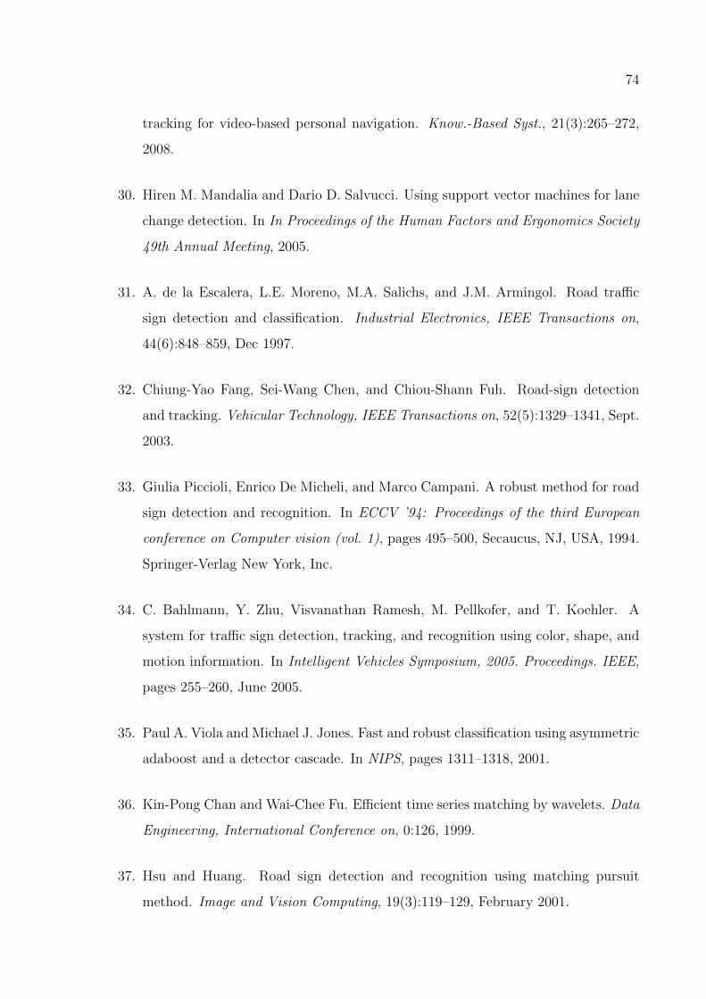
74
tracking for video-based personal navigation. Know.-Based Syst., 21(3):265–272,
2008.
30. Hiren M. Mandalia and Dario D. Salvucci. Using support vector machines for lane
change detection. In In Proceedings of the Human Factors and Ergonomics Society
49th Annual Meeting, 2005.
31. A. de la Escalera, L.E. Moreno, M.A. Salichs, and J.M. Armingol. Road traffic
sign detection and classification. Industrial Electronics, IEEE Transactions on,
44(6):848–859, Dec 1997.
32. Chiung-Yao Fang, Sei-Wang Chen, and Chiou-Shann Fuh. Road-sign detection
and tracking. Vehicular Technology, IEEE Transactions on, 52(5):1329–1341, Sept.
2003.
33. Giulia Piccioli, Enrico De Micheli, and Marco Campani. A robust method for road
sign detection and recognition. In ECCV ’94: Proceedings of the third European
conference on Computer vision (vol. 1), pages 495–500, Secaucus, NJ, USA, 1994.
Springer-Verlag New York, Inc.
34. C. Bahlmann, Y. Zhu, Visvanathan Ramesh, M. Pellkofer, and T. Koehler. A
system for traffic sign detection, tracking, and recognition using color, shape, and
motion information. In Intelligent Vehicles Symposium, 2005. Proceedings. IEEE,
pages 255–260, June 2005.
35. Paul A. Viola and Michael J. Jones. Fast and robust classification using asymmetric
adaboost and a detector cascade. In NIPS, pages 1311–1318, 2001.
36. Kin-Pong Chan and Wai-Chee Fu. Efficient time series matching by wavelets. Data
Engineering, International Conference on, 0:126, 1999.
37. Hsu and Huang. Road sign detection and recognition using matching pursuit
method. Image and Vision Computing, 19(3):119–129, February 2001.
75
38. S.G. Mallat and Zhifeng Zhang. Matching pursuits with time-frequency dictionar-
ies. Signal Processing, IEEE Transactions on, 41(12):3397–3415, Dec 1993.
39. G. Loy and N. Barnes. Fast shape-based road sign detection for a driver assistance
system. In Intelligent Robots and Systems, 2004. (IROS 2004). Proceedings. 2004
IEEE/RSJ International Conference on, volume 1, pages 70–75 vol.1, Sept.-2 Oct.
2004.
40. S. Maldonado-Bascon, S. Lafuente-Arroyo, P. Gil-Jimenez, H. Gomez-Moreno, and
F. Lopez-Ferreras. Road-sign detection and recognition based on support vector
machines. Intelligent Transportation Systems, IEEE Transactions on, 8(2):264–
278, June 2007.
41. C.G. Kiran, L.V. Prabhu, V.A. Rahiman, K. Rajeev, and A. Sreekumar. support
vector machine learning based traffic sign detection and shape classification using
distance to borders and distance from center features. In TENCON 2008 - 2008,
TENCON 2008. IEEE Region 10 Conference, pages 1–6, Nov. 2008.
42. Pedro Gil Jimenez, Saturnino Maldonado Bascon, Hilario Gomez Moreno, Ser-
gio Lafuente Arroyo, and Francisco Lopez Ferreras. Traffic sign shape classifica-
tion and localization based on the normalized fft of the signature of blobs and 2d
homographies. Signal Process., 88(12):2943–2955, 2008.
43. A. De La Escalera, J. M A Armingol, and M. Mata. Traffic sign recognition and
analysis for intelligent vehicles. Image and Vision Computing, 21:247–258, 2003.
44. Aryuanto Soetedjo and Koichi Yamada. K.: Traffic sign classification using ring
partitioned method. IEICE Transactions on Fundamentals of Electronics, Com-
munications and Computer Sciences E, 88:2419–2426, 2005.
45. XW Gao, L. Podladchikova, D. Shaposhnikov, K. Hong, and N. Shevtsova. Recog-
nition of traffic signs based on their colour and shape features extracted using
human vision models. Journal of Visual Communication and Image Representa-

76
tion, 17(4):675–685, 2006.
46. M. R. Luo and R. W. G. Hunt. The structure of the cie 1997 colour appearance
model (ciecam97s). Color Research & Application, 23:138–146, 1998.
47. Hasan Fleyeh. Road and traffic sign color detection and segmentation-a fuzzy
approach. 2005.
48. J. Miura, T. Kanda, and Y. Shirai. An active vision system for real-time traffic
sign recognition. In Intelligent Transportation Systems, 2000. Proceedings. 2000
IEEE, pages 52–57, 2000.
49. M.A. Garcia-Garrido, M.A. Sotelo, and E. Martm-Gorostiza. Fast traffic sign
detection and recognition under changing lighting conditions. In Intelligent Trans-
portation Systems Conference, 2006. ITSC ’06. IEEE, pages 811–816, Sept. 2006.
50. Andrzej Ruta, Yongmin Li, and Xiaohui Liu. Real-time traffic sign recognition
from video by class-specific discriminative features. Pattern Recognition, 43(1):416
– 430, 2010.
51. John Canny. A computational approach to edge detection. Pattern Analysis and
Machine Intelligence, IEEE Transactions on, PAMI-8(6):679–698, Nov. 1986.
52. K. Ratnayake and A. Amer. An fpga-based implementation of spatio-temporal
object segmentation. In Image Processing, 2006 IEEE International Conference
on, pages 3265–3268, Oct. 2006.
53. B. Rabiner, L. Juang. An introduction to hidden markov models. 17(0740-7467):4–
16, 1986.
54. Melanie Mitchell. An Introduction to Genetic Algorithms. The MIT Press, 1998.
55. N. Barnes and A. Zelinsky. Real-time radial symmetry for speed sign detection. In
Intelligent Vehicles Symposium, 2004 IEEE, pages 566–571, June 2004.

77
56. Herbert Bay, Tinne Tuytelaars, and Luc Van Gool. Surf: Speeded up robust
features. In In ECCV, pages 404–417, 2006.
57. David G. Lowe. Object recognition from local scale-invariant features. Computer
Vision, IEEE International Conference on, 2:1150, 1999.
58. Kevin P. Murphy, Antonio B. Torralba, Daniel Eaton, and William T. Free-
man. Object detection and localization using local and global features. In Jean
Ponce, Martial Hebert, Cordelia Schmid, and Andrew Zisserman, editors, Toward
Category-Level Object Recognition, volume 4170 of Lecture Notes in Computer Sci-
ence, pages 382–400. Springer, 2006.
59. Wenhong Zhu, Fuqiang Liu, Zhipeng Li, Xinhong Wang, and Shanshan Zhang. A
vision based lane detection and tracking algorithm in automatic drive. In Com-
putational Intelligence and Industrial Application, 2008. PACIIA ’08. Pacific-Asia
Workshop on, volume 1, pages 799–803, Dec. 2008.
60. Ades project website. http://www.adesproject.com/.
61. Alan Koncar, Holger Janen, and Saman Halgamuge. Gabor wavelet similarity
maps for optimising hierarchical road sign classifiers. Pattern Recognition Letters,
28(2):260 – 267, 2007.
62. Seung Gweon Jeong, Chang Sup Kim, Kang Sup Yoon, Jong Nyun Lee, Jong Il
Bae, and Man Hyung Lee. Real-time lane detection for autonomous navigation. In
Intelligent Transportation Systems, 2001. Proceedings. 2001 IEEE, pages 508–513,
2001.
63. X.W. Gao, L. Podladchikova, D. Shaposhnikov, K. Hong, and N. Shevtsova. Recog-
nition of traffic signs based on their colour and shape features extracted using hu-
man vision models. Journal of Visual Communication and Image Representation,
17(4):675 – 685, 2006.

78
64. Avinoam Borowsky, David Shinar, and Yisrael Parmet. Sign location, sign recog-
nition, and driver expectancies. volume 11, pages 459 – 465, 2008.
65. Miguel S. Prieto and Alastair R. Allen. Using self-organising maps in the detection
and recognition of road signs. Image and Vision Computing, 27(6):673 – 683, 2009.