high-frequency estimates of the natural real rate and
TRANSCRIPT

Finance and Economics Discussion SeriesDivisions of Research & Statistics and Monetary Affairs
Federal Reserve Board, Washington, D.C.
High-Frequency Estimates of the Natural Real Rate and InflationExpectations
Alex Aronovich and Andrew Meldrum
2021-034
Please cite this paper as:Aronovich, Alex, and Andrew Meldrum (2021). “High-Frequency Estimates of theNatural Real Rate and Inflation Expectations,” Finance and Economics DiscussionSeries 2021-034. Washington: Board of Governors of the Federal Reserve System,https://doi.org/10.17016/FEDS.2021.034.
NOTE: Staff working papers in the Finance and Economics Discussion Series (FEDS) are preliminarymaterials circulated to stimulate discussion and critical comment. The analysis and conclusions set forthare those of the authors and do not indicate concurrence by other members of the research staff or theBoard of Governors. References in publications to the Finance and Economics Discussion Series (other thanacknowledgement) should be cleared with the author(s) to protect the tentative character of these papers.

High-Frequency Estimates of the Natural
Real Rate and Inflation Expectations
Alex Aronovich and Andrew Meldrum∗
March 18, 2021
Abstract
We propose a new method of estimating the natural real rate and long-horizon
inflation expectations, using nonlinear regressions of survey-based measures of short-
term nominal interest rates and inflation expectations on U.S. Treasury yields. We
find that the natural real rate was relatively stable during the 1990s and early 2000s,
but declined steadily after the global financial crisis, before dropping more sharply
to around 0 percent during the recent COVID-19 pandemic. Long-horizon inflation
expectations declined steadily during the 1990s and have since been relatively stable
at close to 2 percent. According to our method, the declines in both the natural real
rate and long-horizon inflation expectations are clearly statistically significant. Our
estimates are available at whatever frequency we observe bond yields, making them
ideal for intraday event-study analysis– for example, we show that the natural real
rate and long-horizon inflation expectations are not affected by temporary shocks to
the stance of monetary policy.
Keywords: Natural real rate, nonlinear regression, term structure model.
JEL: E43, G12.
First draft: November 28, 2020. This draft: February 16, 2020.
∗Aronovich, [email protected], Board of Governors of the Federal Reserve System; Meldrum, [email protected], Board of Governors of the Federal Reserve System. We thank Anthony Diercksand Dobrislav Dobrev for useful comments and discussions. The analysis and conclusions set forth are thoseof the authors and do not indicate concurrence by the Board of Governors of the Federal Reserve System orother members of the research staff of the Board.
1

1 Introduction
The natural real rate is an important concept in monetary economics. We can think of
it as being "the real interest rate consistent with output equalling its natural rate and stable
inflation" (Laubach and Williams (2003)) that "provides a neutral benchmark to calibrate
the stance of monetary policy" (Christensen and Rudebusch (2019)). But the natural real
rate cannot be observed directly and it is notoriously diffi cult to estimate. We propose a
novel approach that combines information in surveys of professional forecasters about short-
term nominal interest rates and inflation with information from the yields on U.S. Treasury
securities. Our approach avoids some of the important drawbacks of previous approaches.
Most recent related studies have adopted one of two broad approaches to estimating the
natural real rate. First, following Laubach and Williams (2003), various studies infer the
natural real rate from the dynamics of observed macroeconomic variables. They assume an
IS equation in which real activity reacts to the "interest rate gap" between the observed real
interest rate and the unobserved natural real rate. They further assume that the natural
real rate follows a random walk and that the interest rate gap is expected to close in the
long run. Thus, we can also think of the natural real rate as a long-run concept, since it
corresponds to the long-horizon expectation of the short-term real interest rate. Closely
related studies include Holston, Laubach, and Williams (2017), Lewis and Vazquez-Grande
(2017), and Kiley (2020). Second, studies such as Johannsen and Mertens (2020) and
Christensen and Rudebusch (2019) measure long-horizon expectations of the short-term real
rate using reduced-form time-series models of interest rates; these studies also interpret the
model-implied long-horizon expectations as a proxy for the natural real rate.1 Both broad
approaches have limitations that cause the resulting estimates of natural real rates to be
extremely uncertain: The structural macroeconomic models rely primarily on the correlation
1In addition, various studies estimate long-horizon expectations of short-term nominal interest rates usingtime-series methods (the many examples include Adrian, Crump, and Moench (2013), Bauer and Rudebusch(2020), and Kim and Orphanides (2012)).
2

between economic activity and real interest rates; there is a long literature observing that
this correlation is empirically weak (see, for example, Taylor (1999)). And the more reduced-
form time-series models rely primarily on pinning down the long-run conditional mean of
the real interest rate from the time-series behavior of interest rates, which is known to be
extremely challenging (see, for example, Kim and Orphanides (2012) and Wright (2014)).
Our approach avoids these diffi culties by looking directly at the real interest rate expec-
tations of professional forecasters, as measured by the Blue Chip Economic Indicators and
Blue Chip Financial Forecasts surveys. Survey-based measures of expectations have their
own limitations– we focus on two in particular. First, there is a longstanding literature
observing that surveys likely measure expectations with errors (see, for example, Nordhaus
(1987)). Second, surveys are only observed infrequently, which means that we cannot cleanly
observe the response of the natural real rate to news. To address these two shortcomings, we
estimate nonlinear regressions of survey-based measures of 5-to-10-year-ahead expectations
of the short-term nominal interest rate and Consumer Price Index inflation on the yields on
U.S. Treasury securities. The difference between the fitted values from the regressions for
short-term nominal interest rates and inflation can be interpreted as a measure of the natural
real rate, which is adjusted for measurement error and is available at whatever frequency we
observe Treasury yields.
We find that the natural real rate has declined from around 2.5 percent in January 1990 to
below 0 percent in December 2020. For much of the sample, the natural real rate fluctuated
around an average level of about 2 percent, before declining steadily in the decade following
the global financial crisis. It then dropped more sharply in 2020, following the onset of the
COVID-19 pandemic. We also find that long-horizon inflation expectations have declined
since 1990– from about 4 percent to about 2 percent at the end of our sample. However, this
decline primarily took place during the 1990s; since then long-horizon inflation expectations
have been relatively stable.
Two key assumptions underpin our approach, as well as also other studies that estimate
3
the natural real rate using Treasury yields, such as Christensen and Rudebusch (2019).
First, we assume that all of the information that matters for determining expectations of
future interest rates and inflation is contained in the current term structure of yields on U.S.
Treasury securities– that is, that expectations are "spanned" by the current yield curve.
This spanning assumption is entirely standard in much of the term structure literature and
means that the part of surveys that is unexplained by Treasury yields can be interpreted as
measurement error.2
Second, we assume that the 5-to-10-year-ahead expectation of the short-term real interest
rate is a reasonable proxy for the natural real rate– that is, that it is a suffi ciently long-
horizon expectation that it is not affected by transitory shocks, such as temporary changes
to the stance of monetary policy. Similarly, we would not expect temporary monetary policy
shocks to affect long-horizon inflation expectations if those expectations are well-anchored.
To shed light on the validity of this assumption, we explore the relationship between mon-
etary policy shocks and our estimates of the natural real rate and long-horizon inflation
expectations. Our model is uniquely positioned for this analysis due to its computational
effi ciency: macroeconomic models depend on infrequently published macroeconomic data,
while term structure models require estimation of computationally intensive time series mod-
els; our regression framework enables us to estimate these rates in a fraction of a second at
whatever frequency we observe bond yields. Using standard event study methods and a
data set of high-frequency estimates from 2004 to 2020, we find evidence supporting our
assumption that the natural real rate is not affected by monetary policy shocks. We also
find evidence that long-horizon inflation expectations are not affected by monetary policy
shocks.
Our regression-based approach is closely related to no-arbitrage term structure models
(ATSMs) that are augmented with information from surveys, as in Kim and Orphanides
(2012) and D’Amico, Kim, and Wei (2018) but crucially allows for nonlinearities in the
2Evidence that is supportive of this spanning hypothesis is provided by Bauer and Rudebusch (2017).
4

relationship between surveys and yields. We find that a linear version of our regression
model delivers almost identical results to such a survey-augmented ATSM. The intuition is
simple: while ATSMs also incorporate information about the observed time-series dynamics
of interest rates, this information is only weakly informative about future interest rates (as
shown previously by Kim and Orphanides (2012), among others). And we show nonlinear-
ities are necessary to capture the broad movements in natural real rates and long-horizon
inflation expectations. Moreover, our approach can also deliver results at a tiny fraction of
the complexity and computational cost of a term structure model.
The remainder of the paper proceeds as follows. In Section 2, we explain our nonlinear
regression-based approach. In Section 3, we report our central findings from an application
of this approach to Blue Chip surveys regressed on U.S. Treasury yields. In Section 4, we
explore the relationship between monetary policy shocks and our estimates of the natural
real rate and long-horizon inflation expectations. In Section 5, we shed further light on the
relationship between our approach and no-arbitrage term structure models. In Section 6,
we offer some concluding remarks.
2 Nonlinear Regression Model
In this section, we explain our nonlinear regression-based approach to estimating the
natural real rate and long-horizon inflation expectations. Suppose that we observe a noisy,
survey-based proxy for the 5-to-10-year ahead short-term nominal interest rate (s(60,120)t ) and
inflation. We estimate a model of the form
s(60,120)t = g (xt) + ut, (1)
where xt is an nx × 1 vector of regressors, g (xt) is an unknown scalar valued function of xt,
and ut is a measurement error. The fitted value from equation (1), g (xt), can be interpreted
of a time-t estimate of the expected short-term nominal rate from 5 to 10 years ahead. We
5

estimate an exactly analogous regression for inflation expectations and take the difference
between the fitted expected nominal rate and fitted expected inflation as a proxy for the
natural real rate.
To estimate equation (1), we use the local linear estimator of the function g (xt) for period
t,
g (xt) = e′1 (X′WX)−1
X′Ws, (2)
where s =[s(n)s1 , s
(n)s2 , ..., s
(n)sT
]′is a T ×1 vector of survey observations for periods s1, s2, ..., sT ,
e1 is a nx × 1 vector with the first element equal to 1 and the remaining elements equal to
zero,
X =
1 (xs1 − xt)′
1 (xs2 − xt)′
... ...
1 (xsT − xt)′
, (3)
and W is a sT × sT weighting matrix. We use the local linear regression weighting matrix
W =
nx∏d=1
K(xs1,d−xt,d
bd
)0 ... 0
0nx∏d=1
K(xs2,d−xt,d
bd
)... 0
... ... ... ...
0 0 ...nx∏d=1
K(xsT ,d−xt,d
bd
)
. (4)
Thus, the weightings are determined by the Gaussian kernel function K (.) and the nx
bandwidth parameters {bd}nxd=1, where bd ≥ 0 for all d. Intuitively, very small values of bd
mean that the weighted regression only assigns material weight to the near neighbors of xt,d,
while very large values assign roughly equal weights across the sample. In the case where
bd → ∞ for all d, the regression approaches the linear ordinary least squares estimator (in
Section 3.4, we discuss the importance of allowing for a nonlinear relationship between yields
6

and surveys).
We choose the values of the bandwidth parameters bd optimally, using a standard leave-
one-out cross validation technique. Specifically, we choose b∗d according to
b∗d = arg min{bd}nxd=1
sT∑i=s1
( ui| Ii)2 , (5)
where u(n)i∣∣∣ Ii is the "out-of-sample" squared residual from equation (1), that is, it is esti-
mated using all observations except for si.
3 Estimates of the Natural Real Rate and Long-Horizon
Inflation Expectations
We now turn to our application and results. In Section 3.1, we describe our core data set.
In Section 3.2, we present our estimates of the natural real rate and long-horizon inflation
expectations. In Section 3.3, we compare our estimates with those from other prominent
studies that estimate the natural real rate. In Section 3.4, we demonstrate the importance of
allowing for nonlinearities in the relationship between bond yields and survey-based measures
of expectations. In Section 3.5, we discuss an important advantage of our estimates, which
is that they are available at a higher frequency than previous estimates of the natural real
rate.
3.1 Data
We use survey-based measures taken from the Blue Chip Economic Indicators and Blue
Chip Financial Forecasts surveys published by Wolters Kluwer Legal and Regulatory Solu-
tions U.S. as the dependent variable in our regressions. These surveys ask panels of business
economists for their expectations of various economic and financial variables, including the
3-month U.S. Treasury bill yield, which we use as a proxy for the short-term nominal interest
7

rate, and the year-on-year rate of inflation measured by the Consumer Price Index. We use
the mean forecast across respondents to the survey over a sample from January 1990 to De-
cember 2020. Although both Blue Chip surveys are conducted monthly, we only use the two
editions each year for each survey where the forecast horizon extends beyond the next couple
of years; in recent years, these "long-range" versions of the Economic Indicators surveys have
been conducted in March and October, and of the Financial Forecasts surveys in June and
December. One complication is that the surveys do not ask directly for expectations over
periods of fixed length (such as the next 10 years), but instead ask for the average expec-
tation over a calendar period, such as a particular calendar quarter or year. We therefore
construct estimates of the average expected Treasury bill yield and inflation rate over the
next 5 and 10 years using the linear interpolation method described in Appendix A.
Our regressors are estimates of yields on zero-coupon bonds with maturities of 6 months,
5 years, and 10 years, that is, xt =[y(6)t , y
(60)t , y
(120)t
]′, where y(n)t is the n-month zero-coupon
yield. The zero-coupon yields are based on a smoothed yield curve fitted to the prices of
off-the-run nominal U.S. Treasury securities, as in Gürkaynak, Sack, and Wright (2007).3
We pick three points on the yield curve because a large literature dating back at least to
Litterman and Scheinkman (1991) has shown that three linearly independent combinations
of yields span almost all of the information in the cross section of yields.
3.2 Results
Figure 1 shows resulting estimates of the natural real rate (the red line) and the average
expected inflation rate (the blue line) between 5 and 10 years ahead. The natural real
rate declines from about 2.5 percent in January 1990 to a little below 0 percent in December
2020. However, the decline was not steady over the sample: The natural real rate fluctuated
around a constant mean of about 2 percent until the global financial crisis in 2008. Since
2008, it has declined fairly steadily, but with a sharper drop in early 2020 following the
3Updates of the data set are available at https://www.federalreserve.gov/data/nominal-yield-curve.htm.
8
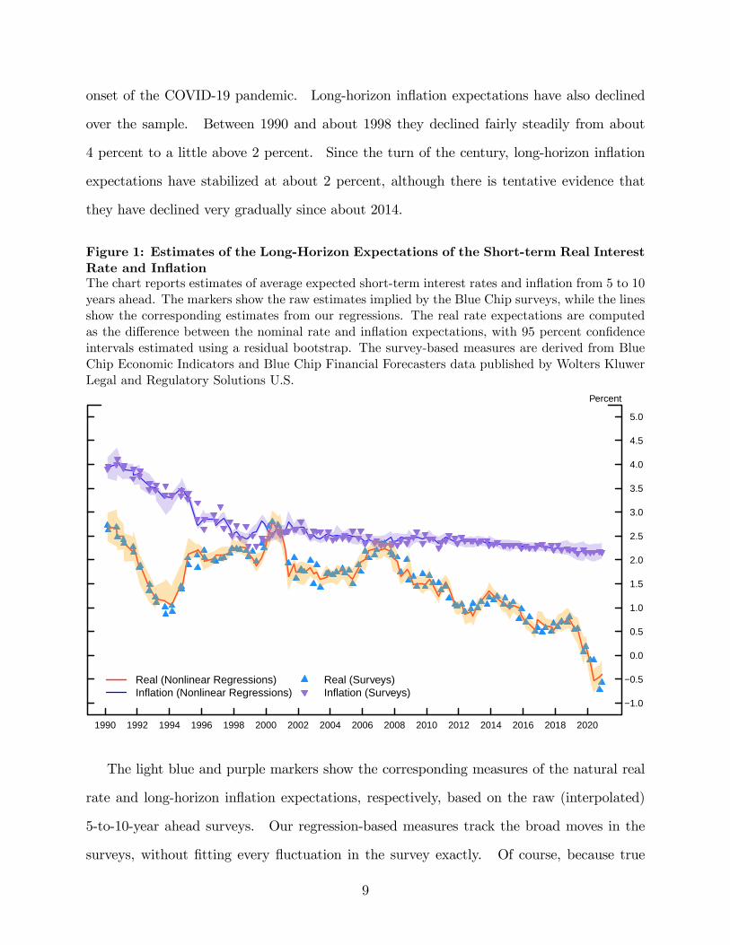
onset of the COVID-19 pandemic. Long-horizon inflation expectations have also declined
over the sample. Between 1990 and about 1998 they declined fairly steadily from about
4 percent to a little above 2 percent. Since the turn of the century, long-horizon inflation
expectations have stabilized at about 2 percent, although there is tentative evidence that
they have declined very gradually since about 2014.
Figure 1: Estimates of the Long-Horizon Expectations of the Short-term Real InterestRate and InflationThe chart reports estimates of average expected short-term interest rates and inflation from 5 to 10years ahead. The markers show the raw estimates implied by the Blue Chip surveys, while the linesshow the corresponding estimates from our regressions. The real rate expectations are computedas the difference between the nominal rate and inflation expectations, with 95 percent confidenceintervals estimated using a residual bootstrap. The survey-based measures are derived from BlueChip Economic Indicators and Blue Chip Financial Forecasters data published by Wolters KluwerLegal and Regulatory Solutions U.S.
Real (Nonlinear Regressions)Inflation (Nonlinear Regressions)
Real (Surveys)Inflation (Surveys)
1990 1992 1994 1996 1998 2000 2002 2004 2006 2008 2010 2012 2014 2016 2018 2020
−1.0
−0.5
0.0
0.5
1.0
1.5
2.0
2.5
3.0
3.5
4.0
4.5
5.0
Percent
The light blue and purple markers show the corresponding measures of the natural real
rate and long-horizon inflation expectations, respectively, based on the raw (interpolated)
5-to-10-year ahead surveys. Our regression-based measures track the broad moves in the
surveys, without fitting every fluctuation in the survey exactly. Of course, because true
9
expectations are unobserved, it is hard to say for sure whether we are appropriately account-
ing for measurement error in the surveys. However, it seems intuitively encouraging that
our model does not match what proved to be a very short-lived decrease in the raw survey
measure of the natural real rate in 1996 and a series of reversals in the early 2000s.
Figure 1 also plots 95 percent confidence intervals computed using a residual bootstrap.4
At first glance, the confidence intervals may appear surprisingly tight given the nature of the
diffi culty in estimating long-horizon expectations of interest rates, with widths in the order
of only 12percentage point. The confidence intervals are generally slightly wider earlier in
the sample than later in the sample, because there are relatively few observations when the
regressor yields were high– as tended to be the case early in the sample. Of course the
reason for the generally tight confidence intervals is that it is possible to explain most of the
variation in surveys using yields. Providing surveys are unbiased, we can be fairly certain
that the decline in long-horizon expectations of short-term real interest rates and inflation
over the sample is statistically significant.
3.3 Comparison with Other Estimates
How do our estimates of the natural real compare with those from other studies? As
discussed above, perhaps the most popular approach for estimating the natural real rate in
recent years has been the approach of Laubach and Williams (2003). In Figure 2, we report
our regression-based estimate in the red line, alongside the Laubach and Williams (2003)
estimates (the purple line) and the estimates from the similar model of Holston et al. (2017).5
4To estimate the confidence intervals around our estimates, we employ a standard bootstrapping proce-dure utilizing residual resampling. At each iteration of the bootstrap, we first randomly sample residualswith replacement from the observed results for each survey date, separately for the nominal and inflationmodels. Adding the resampled residuals to the model-implied fitted values gives us a new bootstrappedset of surveys. Then, for each regression, we re-optimize the bandwidth parameters for the bootstrappedsample and estimate the models. We take the difference between the fitted values from the bootstrappednominal and inflation regressions for the real model results. The 95 percent confidence intervals report therange between the 2.5th and 97.5th percentiles of the estimates from the bootstrap samples.
5We report estimates of the natural real rate from these studies that are smoothed, that is, which estimatethe natural real rate at each point in time using data for the full sample. That is closest in spirit to ourregressions, which use full-sample information.
10

Broadly speaking, the three estimates have some notable similarities: all three decline from
between 2 percent and 3 percent in the early 1990s to between -0.5 percent and 0.5 percent
in December 2020. The models disagree to some extent over the timing of the fall, with the
estimates from the macroeconomic models declining somewhat earlier than our estimates.
One potential explanation for this timing difference could be that the expectations of the
forecasters responding to the Blue Chip survey may have been influenced by the estimates
from these prominent macroeconomic models.
Figure 2: Estimates of the Natural Real Rate: Comparison with Other EstimatesThe chart reports estimates of the natural real rate: our regression-based estimator and two alter-native estimates from macroeconomic models.
RegressionsLaubach and Williams (2003)Holston, Laubach, and Williams (2017)
1990 1992 1994 1996 1998 2000 2002 2004 2006 2008 2010 2012 2014 2016 2018 2020
−1.0
−0.5
0.0
0.5
1.0
1.5
2.0
2.5
3.0
3.5
4.0
Percent
11

3.4 Importance of Nonlinearities
To shed light on how much the nonlinearities in equation (1) matter for our ability to
match surveys, we also estimate a linear version of the model, that is,
s(60,120)t = g0 + g′xxt + ut. (6)
Figure 3 shows how well this linear model matches the raw surveys. The red and blue
lines again show the results for the natural real rate and long-horizon inflation expectations,
respectively, while the pale blue and purple markers show the corresponding raw survey-
based measures. The estimates from the linear model decline over the sample, but the
model is clearly insuffi ciently flexible to match some of the broad movements in the surveys.
In particular, the model is not able to generate the observed pattern in long-horizon inflation
expectations, for which the raw surveys decline steadily in the 1990s before levelling off over
the remainder of the sample. Similarly, the linear model is not able to capture the extent
of the decline in the natural real rate since the global financial crisis.
3.5 Daily Estimates
An important advantage of our estimates of the natural real rates is that they are available
at whatever frequency we observe Treasury yields, whereas previous estimates are typically
only available at a monthly or quarterly frequency. This feature of our estimates has
the potential to make them particularly useful for policymakers and practitioners who are
interpreting higher-frequency movements in Treasury yields. We would intuitively expect
the natural real rate to be slow-moving, with daily changes that are less volatile than changes
in Treasury yields. Similarly, if long-term inflation expectations are well anchored we would
also expect them not to change materially from day to day. Because financial market prices
can fluctuate from day to day, when we compute our estimates at a daily frequency we also
find day-to-day variation. However, we confirm the intuitive result that they are much less
12

Figure 3: The Importance of Nonlinearities: Estimates of Long-Horizon Expectationsof the Short-Term Real Interest Rate and InflationThe chart reports estimates of average expected short-term interest rates and inflation from 5 to10 years ahead. The markers show the raw estimates implied by the Blue Chip surveys, while thelines show the corresponding estimates from linear versions of our regressions. The real rate expec-tations are computed as the difference between the nominal rate and inflation expectations. Thesurvey-based measures are derived from Blue Chip Economic Indicators and Blue Chip FinancialForecasters data published by Wolters Kluwer Legal and Regulatory Solutions U.S.
Real (Linear Regressions)Inflation (Linear Regressions)
Real (Surveys)Inflation (Surveys)
1990 1992 1994 1996 1998 2000 2002 2004 2006 2008 2010 2012 2014 2016 2018 2020
−1.0
−0.5
0.0
0.5
1.0
1.5
2.0
2.5
3.0
3.5
4.0
4.5
5.0
Percent
volatile than financial market prices.
Figure 4 illustrates this result. The gray bars show the empirical distribution of daily
changes in the 5-to-10-year nominal forward rate. As is standard, we can think of this for-
ward rate as reflecting the sum of the average expected short-term real, the average expected
inflation rate, and an additional term premium component that compensates investors for
risks. Most of the variation in the forward rate appears to be accounted for by changes
in term premiums: the variability of daily changes in the expected real rate (the distribu-
tion shown by the red dashed line) and expected inflation (the black line) is much less than
the variability of the raw forward rates. The large majority of daily changes in long-term
13

inflation expectations are between -1 basis point and 1 basis point. The distribution of
daily changes in the long-horizon expectations of the short-term real rate is slightly more
dispersed, although a clear majority of daily changes are between -2 basis points and 2 basis
points. Thus, the daily estimates confirm our prior that long-horizon expectations are not
subject to frequency large daily changes.
Figure 4: Histogram of Daily Changes in Long-Horizon Expectations of Real InterestRates and Inflation Real RateThe chart plots histograms of daily changes in the 5-to-10-year forward rate implied by nominalTreasury yields alongside similar histograms of daily changes in our estimates of 5-to-10-year ex-pectations of the short-term real interest rate and inflation. The probability for each bin on thex-axis refers to the proportion of daily changes falling in the 1-basis-point interval above the axislabel (for example, the bin labeled "0" refers to the range from 0 basis points to 1 basis point). Avery small proportion of daily changes fall outside the plotted range.
5−to−10−year forward rateAverage expected inflationAverage expected short−run real rate
−20 −19 −18 −17 −16 −15 −14 −13 −12 −11 −10 −9 −8 −7 −6 −5 −4 −3 −2 −1 0 1 2 3 4 5 6 7 8 9 10 11 12 13 14 15 16 17 18 19 20 0.0
0.1
0.2
0.3
0.4
Probability
Daily change (basis points)
14

4 Effect of Monetary Policy Shocks on Natural Real
Rates and Long-Horizon Inflation Expectations
As discussed above, a key assumption underpinning our approach to estimating the nat-
ural real rate is that 5-to-10-year ahead real rate expectations are not affected by short-lived
disturbances such as temporary changes in the stance of monetary policy. Unfortunately,
assessing whether this assumption holds in practice is usually challenging because previous
estimates are only available at a monthly or quarterly frequency. However, the fact that our
method can produce estimates at whatever frequency we observe Treasury yields means that
we can identify the effects of monetary policy shocks over narrow windows using standard
event study methods. Similarly, we can also consider whether long-horizon inflation expec-
tations respond to what should be transitory monetary policy shocks. In Section 4.1, we
explain the data set and methodology we employ to conduct event studies, while in Section
4.2, we report our results.
4.1 Event Study Method
To measure whether our estimates the natural real rate are significantly affected by
monetary policy shocks, we estimate a regression of the change in our estimates on measures
of monetary policy shocks:
∆r∗t,t+h = β0 + β1∆zt,t+h + εt,t+h, (7)
where ∆r∗t,t+h is the change in our measure of the natural real rate over a narrow window
between time t and time t+h, ∆zt,t+h is our proxy for the monetary policy shock, and εt,t+h
is an error term. If the slope coeffi cient β1 is significantly different from zero then we would
conclude that the natural real rate is affected by monetary policy shocks. This is an en-
tirely standard event study method, following Gürkaynak, Sack, and Swanson (2005), among
15
others. We estimate exactly analogous regressions for long-term inflation expectations.
As discussed above, our approach for estimating the natural real rate and inflation ex-
pectations framework relies on estimates of zero-coupon yields derived from the prices of
off-the-run U.S. Treasury securities. These off-the-run zero-coupon yields have the advan-
tage of being available at a daily frequency over an extended historical period, but they are
not available at a suffi ciently high intraday frequency to conduct reliable event studies. To
create a higher-frequency proxy for off-the-run zero-coupon yields, we estimate separate lin-
ear regressions of the 6-month, 5-year, and 10-year zero-coupon yields on 2-, 5-, and 10-year
on-the-run yields, which are available to us at a much higher intraday frequency. We cal-
culate these on-the-run yields using data from the BrokerTec exchange for January 2004 to
December 2020; the data are processed in the same way as in Fleming, Mizrach, and Nguyen
(2018) and Fleming and Nguyen (2018).6 We use the fitted values from these regressions
as proxies for the zero-coupon yields. We choose the 2-, 5-, and 10-year yields as regressors
because these are the only maturities that are available throughout our sample. Regressing
zero-coupon yields on these on-the-run yields likely provides a very accurate proxy for intra-
day zero-coupon yields, because the R2 statistics for the daily zero-coupon yields are 0.985
or higher.
To calculate the monetary policy shocks for use in equation (7), we employ the standard
methods described in Gürkaynak et al. (2005): We calculate changes in financial market
prices around FOMC statement releases over our sample. We consider two alternative mea-
sures of monetary policy shocks: First, we use the change in the market-implied expectation
of the federal funds rate after the fourth future Federal Open Market Committee (FOMC)
meeting that occurred around FOMC statement releases between January 2004 and Decem-
ber 2020.7 However, while this is a fairly standard measure of monetary policy surprises,
it may be distorted during much of our sample because short-term interest rates were close
6We use mid quotes from the top level of the BrokerTec order book. Our results do not change materiallyif we instead use realized transaction prices, or if we use ask or bid yields.
7Our results are not materially affected by using rate expectations following other FOMC meetings (weconsider the first through sixth future meetings).
16
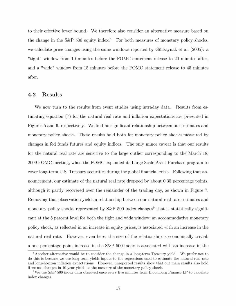
to their effective lower bound. We therefore also consider an alternative measure based on
the change in the S&P 500 equity index.8 For both measures of monetary policy shocks,
we calculate price changes using the same windows reported by Gürkaynak et al. (2005): a
"tight" window from 10 minutes before the FOMC statement release to 20 minutes after,
and a "wide" window from 15 minutes before the FOMC statement release to 45 minutes
after.
4.2 Results
We now turn to the results from event studies using intraday data. Results from es-
timating equation (7) for the natural real rate and inflation expectations are presented in
Figures 5 and 6, respectively. We find no significant relationship between our estimates and
monetary policy shocks. These results hold both for monetary policy shocks measured by
changes in fed funds futures and equity indices. The only minor caveat is that our results
for the natural real rate are sensitive to the large outlier corresponding to the March 18,
2009 FOMC meeting, when the FOMC expanded its Large Scale Asset Purchase program to
cover long-term U.S. Treasury securities during the global financial crisis. Following that an-
nouncement, our estimate of the natural real rate dropped by about 0.35 percentage points,
although it partly recovered over the remainder of the trading day, as shown in Figure 7.
Removing that observation yields a relationship between our natural real rate estimates and
monetary policy shocks represented by S&P 500 index changes9 that is statistically signifi-
cant at the 5 percent level for both the tight and wide window; an accommodative monetary
policy shock, as reflected in an increase in equity prices, is associated with an increase in the
natural real rate. However, even here, the size of the relationship is economically trivial:
a one percentage point increase in the S&P 500 index is associated with an increase in the8Another alternative would be to consider the change in a long-term Treasury yield. We prefer not to
do this is because we use long-term yields inputs to the regressions used to estimate the natural real rateand long-horizon inflation expectations. However, unreported results show that out main results also holdif we use changes in 10-year yields as the measure of the monetary policy shock.
9We use S&P 500 index data observed once every five minutes from Bloomberg Finance LP to calculateindex changes.
17

natural real rate of less than one basis point, for both the tight and wide windows. Thus,
we conclude that there is no evidence that we should be concerned that our proxy for the
natural real rate is being contaminated by the effects of short-lived changes in the stance of
monetary policy.
Figure 5: Relationship between Monetary Policy Shocks and the Natural Real RateThe chart plots changes in financial market prices around FOMC statement releases on the x-axesagainst changes in the natural real rate on the y-axes. The left column (MP4) shows results forfederal funds rate expectations following the fourth future FOMC meeting, as measured by federalfunds futures prices. The right column (SP500) shows results for the S&P 500 equity index. Thetop row shows results for a tight event window from 10 minutes before the statement release to 20minutes after, and the bottom row shows results for a wide event window from 15 minutes beforethe statement release to 45 minutes after. Each black dot represents one FOMC meeting, withthe March 18, 2009 meeting picked out in red. The blue line shows a linear regression line, withthe gray shaded area showing the corresponding 95 percent confidence interval. The estimatedregression equation and the p-value of the slope coeffi cient for the regression equation are reportedin the text inset.
y = − 0.00339 − 0.0542 xp−value = 0.4647
March 18, 2009 FOMC
y = − 0.00148 + 0.0196 xp−value = 0.1796
March 18, 2009 FOMC
y = − 0.00274 − 0.00676 xp−value = 0.2472
March 18, 2009 FOMC
y = − 0.00175 − 0.00354 xp−value = 0.3554
March 18, 2009 FOMC
MP4 SP500
Tight w
indowW
ide window
−1.0 −0.5 0.0 −2 −1 0 1 2 3
−0.3
−0.2
−0.1
0.0
−0.2
−0.1
0.0
Monetary policy shock
Cha
nge
in n
atur
al r
eal r
ate
18

Figure 6: Relationship between Monetary Policy Shocks and Long-Horizon InflationExpectationsThe chart plots changes in financial market prices around FOMC statement releases on the x-axesagainst changes in the long-horizon inflation expectation on the y-axes. The left column (MP4)shows results for federal funds rate expectations following the fourth future FOMC meeting, asmeasured by federal funds futures prices. The right column (SP500) shows results for the S&P500 equity index. The top row shows results for a tight event window from 10 minutes before thestatement release to 20 minutes after, and the bottom row shows results for a wide event windowfrom 15 minutes before the statement release to 45 minutes after. Each black dot represents oneFOMC meeting, with the March 18, 2009 meeting picked out in red. The blue line shows a linearregression line, with the gray shaded area showing the corresponding 95 percent confidence interval.The estimated regression equation and the p-value of the slope coeffi cient for the regression equationare reported in the text inset.
y = 0.000239 + 0.00743 xp−value = 0.6385
March 18, 2009 FOMC
y = − 0.00014 − 0.00276 xp−value = 0.4539
March 18, 2009 FOMC
y = 0.000354 − 0.0024 xp−value = 0.05294
March 18, 2009 FOMC
y = 0.000185 − 0.00147 xp−value = 0.1249
March 18, 2009 FOMC
MP4 SP500
Tight w
indowW
ide window
−1.0 −0.5 0.0 −2 −1 0 1 2 3
−0.04
−0.02
0.00
0.02
−0.04
−0.02
0.00
0.02
Monetary policy shock
Cha
nge
in lo
ng−
horiz
on in
flatio
n ex
pect
atio
ns
19

Figure 7: Natural Real Rate on March 18, 2009
FO
MC
Sta
tem
ent R
elea
se
1.0
1.1
1.2
1.3
1.4
11:00 12:00 13:00 14:00 15:00 16:00 17:00Time
Per
cent
5 Comparison with Affi ne Term Structure Models
In this section, we shed further light on the relationship between our estimates and
those obtained from no-arbitrage term structure models. In Section 5.1 we show that term
structure models estimated using only the history of interest rates deliver highly uncertain
and implausible estimates of 5-to-10-year ahead interest rate expectations. However, in
Section 5.2, we show that augmenting the term structure model with information from
surveys delivers essentially the same results as linear versions of our regressions– but at
considerable additional computational cost.
20

5.1 Time-Series Estimates: No-Arbitrage Term Structure Models
As discussed above, an alternative approach to estimating financial market participants’
expectations of the short-term interest rates and inflation is to use an econometric model
that describes the time-series properties of interest rates or inflation. A standard approach
is to use the dynamic no-arbitrage ATSM of Duffee (2002). The many examples include
Christensen, Diebold, and Rudebusch (2011), Adrian et al. (2013), and Abrahams, Adrian,
Crump, Moench, and Yu (2016). Focusing on the case of nominal interest rates, in an ATSM
the short-term interest rate (rt) takes the form
rt = δ0 + δ′xxt, (8)
where xt is an nx × 1 vector of bond yields observed at month t, δ0 is a scalar and δx is an
nx × 1 vector. The factors follow the first-order vector autoregression
xt+1 = µ+ Φxt + vt, (9)
where µ is an nx×1 vector, Φ is an nx×nx matrix, and vt ∼ N (0,ΣΣ′) is an nx×1 vector
of shocks. Thus, the conditional expectation of the average short-term real interest from
5 to 10 years ahead is an affi ne function of xt. Estimation can take place using standard
maximum likelihood techniques. Appendix B provides additional details about the model.
We estimate the above model using end-month Treasury yields with maturities of 6
months, 5 years, and 10 years, that is, xt =[y(6)t , y
(60)t , y
(120)t
]′, over a sample period from
January 1990 to July 2020. The pink line in Figure 8 shows the model-implied fitted value
of 5-to-10-year ahead short-term nominal rate expectations, with the gray shading showing
the corresponding 95 percent confidence interval, computed using a bootstrap procedure.10
10Specifically, we perform 1,000 draws of samples of yields with the same number of months as our esti-mation sample. We use a residual block bootstrap with a block length of 60 months and construct yieldsusing equation (9). For each simulated sample, we estimate the model parameters separately.
21

We highlight two important results: First, the point estimate of the expected short rate is
substantially lower than our regression-based estimate, shown in the blue line; while surveys
may measure expectations with some error, it seems implausible to us that surveys would
be this far away from true expectations. Second, the parameter uncertainty for the term
structure model is extremely wide, such that the 95 percent confidence interval for 5-to-10-
year-ahead expectations cover a region about four percentage points wide. Thus, we cannot
with material confidence reject the hypothesis that the short rate expectation was constant
over the sample.
Figure 8: Estimates of Long-Horizon Nominal Interest Rate Expectations: Compari-son with Standard ATSMThe chart reports estimates of the average expected short-term nominal interest rate from 5 to 10years ahead. The blue line shows estimates based on our regressions. The pink line shows estimatesfrom a standard ATSM, with the gray shaded area showing the corresponding 95 percent confidenceinterval computed using a block bootstrap.
RegressionsTerm structure model point estimatesTerm structure model 95% confidence interval
1990 1992 1994 1996 1998 2000 2002 2004 2006 2008 2010 2012 2014 2016 2018 2020
−2.0
−1.0
0.0
1.0
2.0
3.0
4.0
5.0
6.0
7.0
8.0
Percent
22

5.2 Survey-Augmented Term Structure Models
The reason that estimates of the natural real rate from a standard ATSM are so uncertain
is well-known: bond yields are extremely persistent, so it is hard to pin down the parameters
that determine their time-series dynamics (µ andΦ in equation (9)) using just a few decades’
worth of data. Kim and Orphanides (2012) therefore propose to incorporate additional
information from survey expectations within an ATSM to help pin down those time-series
parameters; D’Amico et al. (2018) apply the same technique to a model that also decomposes
nominal interest rates into real and inflation components.
We can incorporate our survey-based measure of 5-to-10-year ahead short-term real rate
expectations into the above ATSM in the same way as in Kim and Orphanides (2012). We
assume that our survey-based measure of the expected average short-term nominal interest
rate from 5 to 10 years ahead (s(60,120)t ) measures expectations with independent Normally-
distributed measurement errors, that is
s(60,120)t = γ0 + γ ′xxt + wt, (10)
where the scalar γ0 and an nx× 1 vector γx are determined by the structural parameters in
equations (8), and (9), wt ∼ N (0, rs), and E [wtvt] = 0. Estimation can still proceed by
maximum likelihood. Appendix B provides further details.
Figure 9 shows the results for the survey-augmented term structure model, correspond-
ing to those in Figure 8. The point estimate from the survey-augmented term structure
model comes reasonably close to tracking our regression-based estimate, and hence the raw
surveys, suggesting that we should consider it far more plausible than the estimate from a
standard term structure model. Moreover, the 95 percent confidence interval is now much
narrower because the surveys help to pin down the parameters that determine the time-series
properties of interest rates with much greater precision.
How should we think about the differences between our regression-based approach and
23

Figure 9: Estimates of Long-Horizon Nominal Interest Rate Expectations: Compari-son with Survey-Augmented ATSMThe chart reports estimates of the average expected short-term nominal interest rate from 5 to 10years ahead. The dark blue line shows estimates based on our regressions. The pink line showsestimates from a survey-augmented ATSM, with the gray shaded area showing the corresponding95 percent confidence interval computed using a block bootstrap. The pale blue line shows anestimate from a linear regression of surveys on yields (this line is usually hidden behind the pinkline).
Nonlinear regressionsLinear regressionsSurvey−augmented term structure model point estimatesSurvey−augmented term structure model 95% confidence interval
1990 1992 1994 1996 1998 2000 2002 2004 2006 2008 2010 2012 2014 2016 2018 2020
0.0
1.0
2.0
3.0
4.0
5.0
6.0
7.0
8.0
Percent
a term structure model approach? There are four differences between the two approaches.
First, our regressions use yields to fit contemporaneous survey-based expectations, whereas
the term structure model needs to trade-off the fit to contemporaneous surveys with the
need to match the observed time-series properties of interest rates. Second, a term struc-
ture model imposes cross-equation restrictions in order to rule out the possibility of arbi-
trage profits. Third, the term structure model imposes a distributional assumption on the
measurement error wt. And fourth, our regression relaxes the assumption of linearity; as
discussed above, equation (10) can be interpreted as the limiting case of equation (1), in
which the functional mapping from yields to expected future short rates is linear.
24

In order to shed light on the importance of these differences, the pale blue line in Figure 9
plots an estimate from a linear version of the regression in equation (1). The estimates from
the term structure model and the linear regression are virtually identical, which suggests that
the only difference between our regressions and the survey-augmented term structure model
that matters is allowing for nonlinearities. The reasons why the other differences between
the approaches are unimportant are straightforward to understand. It is well-known that
imposing no-arbitrage restrictions makes little difference to conditional expectations of yields
(see, for example, Duffee (2011)). And it is also well-known that there is little information
about future interest rates in their past behavior; indeed, that was exactly the rationale of
Kim and Orphanides (2012) for including surveys in term structure models in the first place.
Thus, the value of term structure models for gaining insights into long-horizon interest rate
expectations seems fairly limited: if we omit surveys from term structure models we obtain
estimates that are highly uncertain and potentially implausible, and if we include surveys we
end up with a model that is unnecessarily complicated, because we could just as well regress
long-horizon surveys on yields. If all we are interested in is long-horizon expectations of
interest rates, why go to the trouble of estimating a term structure model when we can just
estimate a linear regression of surveys on yields?
6 Conclusion
We construct new estimates of the natural real rate and long-horizon inflation expecta-
tions derived from nonlinear regressions of survey forecasts of interest rates and inflation on
U.S. Treasury yields. Our estimates provide an alternative to previous estimates from stud-
ies that use structural macroeconomic and reduced-form time-series models, and avoid some
of the drawbacks of those approaches. We additionally provide evidence that the natural
real rate and long-horizon inflation expectations are not affected by temporary shocks to the
stance of monetary policy. Finally, we show that our estimates are closely related to those
25

from dynamic term structure models that are augmented with survey forecasts, but have the
advantage of allowing for greater flexibility in the relationship between yields and short rate
expectations, as well as being far easier to compute.
References
Abrahams, M., T. Adrian, R. K. Crump, E. Moench, and R. Yu. “Decomposing Real and Nominal
Yield Curves.” Journal of Monetary Economics, 84 (2016), 182—200.
Adrian, T., R. K. Crump, and E. Moench. “Pricing the Term Structure with Linear Regressions.”
Journal of Financial Economics, 110 (2013), 110—138.
Bauer, M. D. and G. D. Rudebusch. “Resolving the Spanning Puzzle in Macro-Finance Term
Structure Models.” Review of Finance, Vol. 21 (2017), 511—553.
Bauer, M. D. and G. D. Rudebusch. “Interest Rates under Falling Stars.” American Economic
Review, 110 (2020), 1316—1354.
Christensen, J. H. E., F. X. Diebold, and G. D. Rudebusch. “The Affi ne Arbitrage-Free Class of
Nelson-Siegel Term Structure Models.” Journal of Econometrics, 164 (2011), 4—20.
Christensen, J. H. E. and G. D. Rudebusch. “A New Normal for Interest Rates? Evidence from
Inflation-Indexed Debt.” The Review of Economics and Statistics, 101 (2019), 933—949.
D’Amico, S., D. H. Kim, and M. Wei. “Tips from TIPS: The Informational Content of Treasury
Inflation-Protected Security Prices.” Journal of Financial and Quantitative Analysis, 53 (2018),
395—436.
Duffee, G. R. “Term Premia and Interest Rate Forecast in Affi ne Models.” Journal of Finance, 57
(2002), 405—443.
Duffee, G. R. “Forecasting with the Term Structure: The Role of No-Arbitrage Restrictions.”
Working paper.
26

Fleming, M., B. Mizrach, and G. Nguyen. “The Microstructure of a U.S. Treasury ECN: The
BrokerTec Platform.” Journal of Financial Markets, 40 (2018), 2—22.
Fleming, M. J. and N. Nguyen. “Price and Size Discovery in Financial Markets: Evidence from
the U.S. Treasury Securities Market.” The Review of Asset Pricing Studies, 9 (2018), 256—295.
Gürkaynak, R. S., B. Sack, and E. T. Swanson. “Do Actions Speak Louder Than Words? The
Response of Asset Prices to Monetary Policy Actions and Statements.” International Journal of
Central Banking, 1 (2005), 55—92.
Gürkaynak, R. S., B. Sack, and J. H. Wright. “The U.S. Treasury Yield Curve: 1961 to the
Present.” Journal of Monetary Economics, 54 (2007), 2291—2304.
Holston, K., T. Laubach, and J. C. Williams. “Measuring the Natural Rate of Interest: International
Trends and Determinants.” Journal of International Economics, 108 (2017), S59—S75.
Johannsen, B. K. and E. Mertens. “A Time Series Model of Interest Rates with the Effective Lower
Bound.” Journal of Money, Credit and Banking, forthcoming.
Joslin, S., K. J. Singleton, and H. Zhu. “A New Perspective on Gaussian Dynamic Term Structure
Models.” Review of Financial Studies, 24 (2011), 926—970.
Kiley, M. T. “What Can the Data Tell Us about the Equilibrium Real Interest Rate?” International
Journal of Central Banking, 62 (2020), 181—209.
Kim, D. H. and A. Orphanides. “Term Structure Estimation with Survey Data on Interest Rate
Forecasts.” Journal of Financial and Quantitative Analysis, 47 (2012), 241—272.
Laubach, T. and J. C. Williams. “Measuring the Natural Rate of Interest.” The Review of Eco-
nomics and Statistics, 85 (2003), 1063—1070.
Lewis, K. F. and F. Vazquez-Grande. “Measuring the Natural Rate of Interest: Alternative Speci-
fications.” Federal Reserve Board Finance and Economics Discussion Series, 2017-059.
Litterman, R. and J. Scheinkman. “Common factors affecting bond returns.” Journal of Fixed
Income, Vol. 1 (1991), 54—61.
27

Nordhaus, W. D. “Forecasting Effi ciency: Concepts and Applications.” Review of Economics and
Statistics, 69 (1987), 667—674.
Taylor, M. P. “Real Interest Rates and Macroeconomic Activity.” Oxford Review of Economic
Policy, 15 (1999), 95—113.
Wright, J. H. “Term Premia and Inflation Uncertainty: Empirical Evidence from an International
Panel Dataset: Reply.”American Economic Review, 104 (2014), 338—341.
28

Appendix A: Constructing Constant-Horizon Surveys
We use the biannual long-horizon Blue Chip Economic Indicators and Blue Chip Financial
Forecasts surveys of 3-month Treasury bill yield and CPI inflation expectations. In recent
years, the long-horizon Financial Forecasts have been published in June and December and
the Economic Indicators in March and October, although the precise timings have varied
somewhat over the sample. Blue Chip does not routinely provide the dates on which
the surveys were submitted by respondents, only the dates the results were published. For
greater precision, we estimate the survey dates based on recent practice regarding publication
lags. In the case of long-horizon Blue Chip Financial Forecasts, the surveys are published
on the first of the month. For these, we label the survey date as the previous Wednesday
before the last business day of the month. If the last business day of the previous month is a
Thursday or Friday, we take the Wednesday of the prior week. Some adjustments are made
for the January survey due to the holiday season: the previous Wednesday from Christmas
Day is calculated. Blue Chip Economic Indicators, on the other hand, are published on the
tenth of the month. For these, we simply take the date three business days before the tenth.
The surveys ask respondents for their average expectations of the Treasury bill yield
and inflation over various calendar periods, starting with the current calendar quarter and
ending with a period ending with a period covering the sixth to eleventh calendar years
ahead. We start by computing the mean expectations across survey respondents for each
of these reference periods. We then interpolate the average expectations for these calendar
periods to estimate expectations over constant horizons of 5 and 10 years, assuming that the
expected value at the mid-point of the reference period is equal to the average value over
the reference period. In some editions of the survey, the first reference point covered by
the survey has already started by the time the survey is taken; in this case, we construct
a purely forward-looking expectation by accounting for the realized Treasury bill yield or
inflation since the beginning of the reference period. In some other editions of the survey,
29

the first reference period has not started by the time the survey is taken; in this case, we
assume the Treasury bill yield is expected to remain constant at its most recent value until
the start of the first reference period, and that the expectation for inflation over the period
until the first reference period is the same as the average expectation in the first reference
period.
Our interpolation also requires us to make an assumption about the expected value of
the Treasury bill yield and inflation at the end of the final reference period. We assume
that this expectation is the same as the average expectation for the final reference period.
We use the interpolated 5- and 10-year expectations to calculate survey respondents’
expectations of the average Treasury bill yield and inflation over a period from 5 to 10
years ahead. We finally take the difference between the Treasury bill expectation and
inflation expectation to represent respondents’expectations of 5-to-10-year ahead real rate
expectations, that is, the natural real rate.
Appendix B: Affi ne Term Structure Model
In addition to equations (8) and (9), we also assume that xt follows a first-order vector
autoregression under the equivalent risk-neutral probability measure (denoted Q):
xt+1 = µQ + ΦQxt + vQt (11)
where µQ is an nx × 1 vector, ΦQ is an nx × nx matrix, and vQt ∼ N (0,ΣΣ′) is an nx × 1
vector of shocks. Under the assumption of no arbitrage, we can show that the yield on an
n-period bond (y(n)t ) is given by
y(n)t = − 1
n(an + b′nxt) , (12)
30

where
an = an−1 + b′n−1µQ +
1
2b′n−1ΣΣ′bn−1 − δ0 and (13)
b′n = b′n−1ΦQ − δx. (14)
See, for example, Joslin, Singleton, and Zhu (2011) for further details. To ensure parameter
identification, we impose the normalization restrictions as in Joslin et al. (2011). We as-
sume that the 6-month, 5-year, and 10-year yields are measured without error. Maximum
likelihood estimation the proceeds straightforwardly as in Joslin et al. (2011).
The conditional expectation of the average short-term interest from 5 to 10 years ahead
is given by
Et
[1
60
119∑i=60
rt+i
]=
δ0 + δ′x (I−Φ)−1µ
+ 160δ′x (I−Φ)−2
(Φ120−Φ60
)µ
+ 160δ′x (I−Φ)−1 (Φ60 −Φ120) xt
. (15)
To augment the standard ATSM with a long-horizon survey expectation, we follow Kim and
Orphanides (2012) and assume that the average expected short-term interest rate from 5 to
10 years ahead measures expectations with an error wt, as in 10, where the coeffi cients γ0
and γx are given by equation (15). Thus, there is one additional parameter to be estimated
by maximum likelihood (rs).
31