on time-frequency analysis of heart rate - repub
TRANSCRIPT

ON TIME-FREQUENCY ANALYSIS OFHEART RATE VARIABILITY
Huibert Goosen van Steenis


ON TIME-FREQUENCY ANALYSIS OFHEART RATE VARIABILITY
OVER TIJD-FREQUENTIE ANALYSE VANHARTRITME VARIABILITEIT
Proefschrift
ter verkrijging van de graad van doctoraan de Erasmus Universiteit Rotterdam
op gezag van de Rector Magnificus
Prof.dr.ir. J.H. van Bemmel
en volgens het besluit van het College voor Promoties.
De openbare verdediging zal plaatsvinden opwoensdag 30 oktober 2002 om 15.45 uur
door
Huibert Goosen van Steenisgeboren te Herwijnen
Promotiecommissie
Promotoren Prof.dr. M.W. HengeveldProf.ir. K.H. Wesseling
Overige leden Prof.dr.ir. N. BomDr.ir. L.J.M. MulderDr. J.A. Kors
Copromotor Dr. J.H.M. Tulen
De werkzaamheden beschreven in dit proefschrift werden uitgevoerd op de afdelingPsychiatrie van het Erasmus MC. De afdeling Psychiatrie wil ik bedanken voor definanciële bijdrage in de kosten van dit proefschrift.
Het gedicht van Ida Gerhardt werd geplaatst met de welwillende toestemming vanEm. Querido's Uitgeverij b.v., Amsterdam.
Drukwerk: Ridderprint offsetdrukkerij b.v., Ridderkerk.
Copyright © 2002 by H.G. van SteenisAll rights reserved. No part of this thesis may be reproduced or transmitted in anyform or by any means, electronic or mechanical, including photocopying, recording orany information storage and retrieval system, without written permission of thepublisher.
ISBN 90-9016246-1

Spreuk bij het werk
Als ik nu in dit landmaar wat alléén mag blijven,dan zal de waterkanthet boek wel voor mij schrijven.
Dit is wat ik behoefen hiertoe moest ik komen,het simpele vertoefbij dit gestadig stromen.
Het water gaat voorbij,wiss’lend gelijk gebleven, -het heeft stilaan in mijeen nieuw begin geschreven.
Ik weet met zekerheid,hier vind ik vroeg of laterhet woord dat mij bevrijdten levend is als water.
Ida Gerhardt
In herinnering:Vader 28-03-2002Moeder 12-10-2000Rien 22-11-1988


Contents page
Chapter 1 Introduction 11
Chapter 2 Heart rate variability and its analysis 23
Chapter 3 Heart rate variability spectra based on non-equidistantsampling: the spectrum of counts and the instantaneous heart ratespectrumMedical Engineering and Physics 16:355-362, 1994
39
Chapter 4 Quantification of autonomic cardiac regulation in psycho-pharmacological researchIn: Measurement of heart rate and blood pressure variability in man.Methods, mechanisms and clinical applications of continuous finger bloodpressure measurement. A.J. Man in 't Veld, G.A. van Montfrans, G.J.Langewouters, K.I. Lie, G. Mancia (eds.). Alphen aan den Rijn: VanZuiden Communications BV, The Netherlands, 1995, chapter 8, pp:61-72
61
Chapter 5 Examining nonequidistantly-sampled cardiovascular timeseries by means of the Wigner-Ville distributionIn: Computers in psychology: applications, methods, and instrumentation.Maarse FJ, Akkerman AE, Brand AN, Mulder LJM, and Van der Stelt MJ(eds). Lisse: Swets & Zeitlinger chapter 13, pp:151-166, 1994. ISSN0925-9244
79
Chapter 6 The exponential distribution applied to nonequidistantlysampled cardiovascular time seriesComputers and Biomedical Research 29:174-193, 1996
99
Chapter 7 Quantification of the dynamic behavior over time of narrow-band components present in heart rate variability by means of theinstantaneous amplitude and frequencySubmitted
127
Chapter 8 The instantaneous frequency of cardiovascular time series:a comparison of methodsComputer Methods and Programs in Biomedicine, accepted
161
Chapter 9 Time-frequency parameters of heart rate variability – usinginstantaneous amplitude and frequency to unravel the dynamics ofcardiovascular control processesIEEE Engineering in Medicine and Biology Magazine, in press
187
Chapter 10 Summary and concluding remarksSamenvatting
221227
Appendix Time-frequency analysisGlossaryAbbreviations
241265274
Dankwoord 277
Curriculum Vitae 279
List of publications 280

CHAPTER 1INTRODUCTION


Introduction - 11 -
1 Background
The human heart does not beat in a constant rhythm, but there are fluctuations intime between two consecutive heartbeats (see figure 1). These fluctuations arespontaneous, or they can be evoked by physical or mental stimulation or bypharmacological interventions. Heart rate is the number of heartbeats per minute.Thus the heart rate shows both random and apparent periodical fluctuations withvariable amplitude and frequency (see figures 2A,3A). These beat-to-beatfluctuations in heart rate are called heart rate variability (HRV) (Task Force p:354,1996).
Although the causes of HRV are still debated, the periodical fluctuations inheart rate are frequently studied to obtain quantitative estimates of sympathetic andparasympathetic processes of neurocardiac function. It has been demonstrated thatHRV follows a 1/f spectral course down to frequencies of 10-5 Hz (Kobayashi et al.,1982; Di Rienzo et al., 1995). The beat-to-beat fluctuations in heart rate present inperiods up to several minutes (2-5 min) are called short-term variability.
ECG
0 0.5 1 1.5 2 2.5 3 3.5 4 4.5 5 5.5 6time (s)
IBI =914 ms
IBI =680 ms
Figure 1. Example of an ECG recording: 6 s recording of a healthy woman of 36years. IBI = interbeat interval.

- 12 - Chapter 1
HR (supine rest)
0.8
1
1.2
1.4
1.6
1.8
0 50 100 150 200 250 300time (s)
Hz
A
PSD (supine rest)
020406080
100120140160180
0 0.1 0.2 0.3 0.4 0.5frequency (Hz)
Hz^
2/H
z
B
Figure 2. Heart rate (HR). A: an example of an equidistantly sampled low-passfiltered cardiac event series (see chapter 2) of about 5 min during supine rest,recorded from a healthy male volunteer; mean heart rate is 72 beats per minute.B: the corresponding power spectral density (PSD) function.

Introduction - 13 -
HR (standing)
0.8
1
1.2
1.4
1.6
1.8
0 50 100 150 200 250 300time (s)
Hz
A
PSD (standing)
020406080
100120140160180
0 0.1 0.2 0.3 0.4 0.5frequency (Hz)
Hz^
2/H
z
B
Figure 3. Heart rate (HR). A: a low-pass filtered cardiac event series of about 5min during orthostatic challenge, recorded from the same person as shown infigure 2; mean heart rate is 87 beats per minute. B: the corresponding powerspectral density (PSD) function.

- 14 - Chapter 1
In the range of short-term variability, three peaks can often be distinguished atfrequencies near 0.04, 0.1, and 0.3 Hz (see figures 2B,3B) (e.g., Hyndman et al.,1971; Sayers, 1973; Kitney, 1975; Akselrod et al., 1981; Kamath et al., 1993; TaskForce, 1996). The first peak, at 0.04 Hz, is of uncertain origin. The 0.1 Hz peak isprobably mediated by the baroreflex and reflects the variable sympathetic tone of theautonomic nervous system. The peak near 0.3 Hz may reflect parasympathetic(vagal) tone linked with respiration. In the study of HRV, these peaks are called thecharacteristic frequency components, bands, or rhythms. It has been shown that theratio of the powers of the heart rate fluctuations in the last two mentioned frequencyareas might be indicative of a sympathovagal balance (e.g., Malliani et al., 1991;Parati et al., 1995). Several closed-loop blood pressure control models have been putforward to explain the short-term variations in heart rate in terms of baroreflex and/orcardiopulmonary reflexes (e.g., Wesseling et al., 1985; Ten Voorde, 1992; Van Roon,1998).
In clinical research, most attention has been paid to the study of HRV. HRVcan be derived non-invasively from a surface ECG. As a non-invasive tool, the studyof HRV has provided valuable information regarding neurocardiac functioning inautonomic nervous system diseases such as neonatal autonomic developmentaldysfunction, autonomic neuropathy (e.g., diabetes mellitus, autonomic failure),hypertension, heart failure, and coronary heart disease. For instance, population-based studies have indicated that reduced HRV, primarily due to reduced vagaleffectiveness, predicts cardiac events, cardiovascular mortality, and the onset ofhypertension (Bigger et al., 1993; Tsuji et al., 1996; Singh et al., 1998; Kikuya et al.,2000).
In affective and anxiety disorders, abnormalities of the autonomic nervoussystem and a higher-than-expected rate of sudden death from cardiac disease havebeen reported (e.g., Malzberg, 1937; Black et al., 1985; Hayward, 1995). Withinpsychiatric research, HRV-analysis has been applied to assess if dysfunctions insympathetic and parasympathetic neurocardiac regulation may explain thesephenomena. Several clinical studies have demonstrated that depressed patientsshow decreased HRV, possibly due to vagal withdrawal (Dalack et al., 1990; Miyakiet al., 1991). However, other studies only found limited evidence for alterations inHRV in depressed patients (Yeragani et al., 1991; Tulen et al., 1996). The issue ofcomorbidity between cardiac diseases and psychiatric symptoms is complicated toresolve. This may be due to the cardiovascular (side-)effects of many psychoactivedrugs, such as tricyclics and MAO-Is. Furthermore, the presence of cardiovascular
Introduction - 15 -
risk factors, e.g., smoking, reduced physical activity, and altered lipid levels, in manypsychiatric populations also complicates this issue.
2 Why time-frequency analysis?
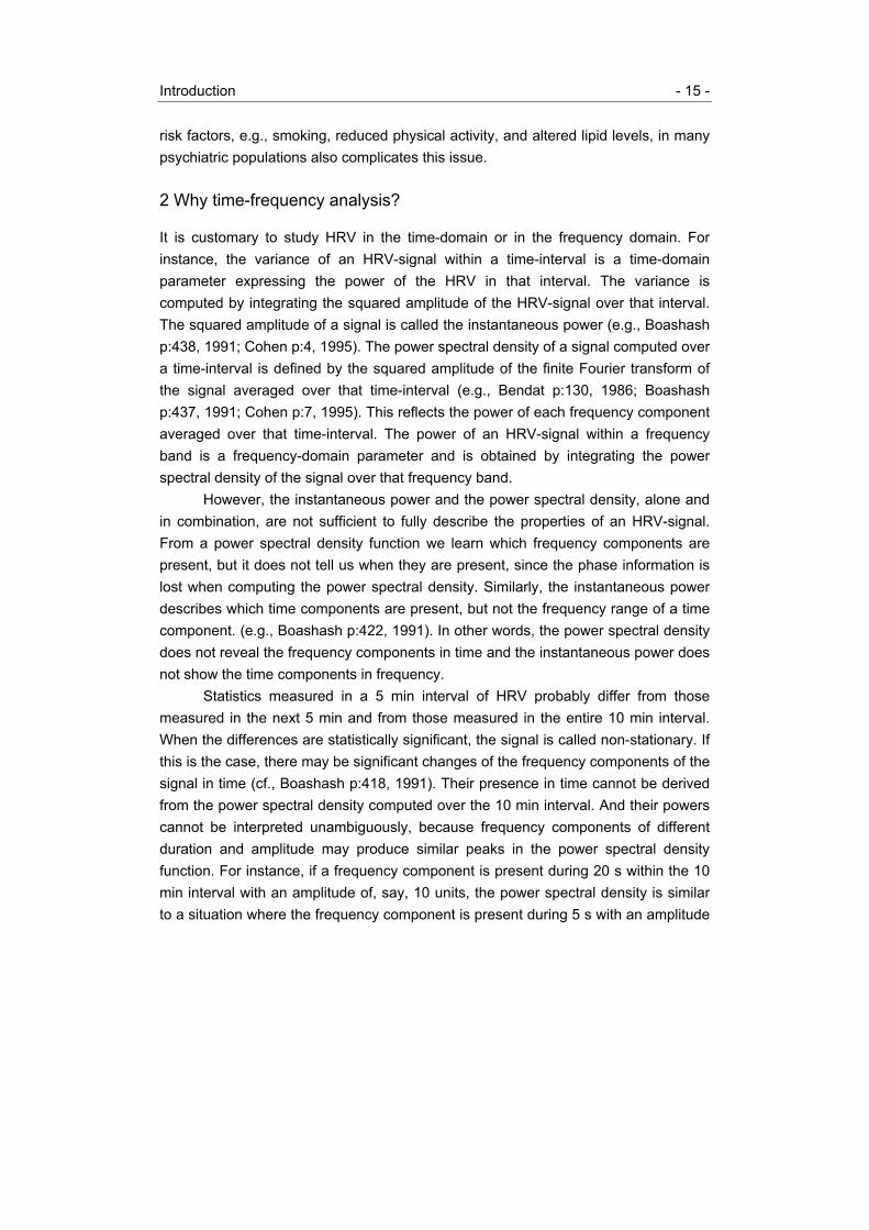
It is customary to study HRV in the time-domain or in the frequency domain. Forinstance, the variance of an HRV-signal within a time-interval is a time-domainparameter expressing the power of the HRV in that interval. The variance iscomputed by integrating the squared amplitude of the HRV-signal over that interval.The squared amplitude of a signal is called the instantaneous power (e.g., Boashashp:438, 1991; Cohen p:4, 1995). The power spectral density of a signal computed overa time-interval is defined by the squared amplitude of the finite Fourier transform ofthe signal averaged over that time-interval (e.g., Bendat p:130, 1986; Boashashp:437, 1991; Cohen p:7, 1995). This reflects the power of each frequency componentaveraged over that time-interval. The power of an HRV-signal within a frequencyband is a frequency-domain parameter and is obtained by integrating the powerspectral density of the signal over that frequency band.
However, the instantaneous power and the power spectral density, alone andin combination, are not sufficient to fully describe the properties of an HRV-signal.From a power spectral density function we learn which frequency components arepresent, but it does not tell us when they are present, since the phase information islost when computing the power spectral density. Similarly, the instantaneous powerdescribes which time components are present, but not the frequency range of a timecomponent. (e.g., Boashash p:422, 1991). In other words, the power spectral densitydoes not reveal the frequency components in time and the instantaneous power doesnot show the time components in frequency.
Statistics measured in a 5 min interval of HRV probably differ from thosemeasured in the next 5 min and from those measured in the entire 10 min interval.When the differences are statistically significant, the signal is called non-stationary. Ifthis is the case, there may be significant changes of the frequency components of thesignal in time (cf., Boashash p:418, 1991). Their presence in time cannot be derivedfrom the power spectral density computed over the 10 min interval. And their powerscannot be interpreted unambiguously, because frequency components of differentduration and amplitude may produce similar peaks in the power spectral densityfunction. For instance, if a frequency component is present during 20 s within the 10min interval with an amplitude of, say, 10 units, the power spectral density is similarto a situation where the frequency component is present during 5 s with an amplitude
- 16 - Chapter 1
of 20 units. Thus the need arises for a description that represents the power of thesignal simultaneously in the time- and frequency-domains. Such time-frequencyrepresentations are often called ‘distributions’ for historical reasons. The phasespectrum of the raw signal contains the information that is necessary to localize thefrequency components in time. Especially, the instantaneous frequency is a means tolocalize the frequency components in time. Therefore, the phase information of theraw signal is included in the computation of a time-frequency representation. Time-frequency signal analysis does not assume stationarity, whereas power spectralanalysis does (e.g., Boashash p:418, 1991).
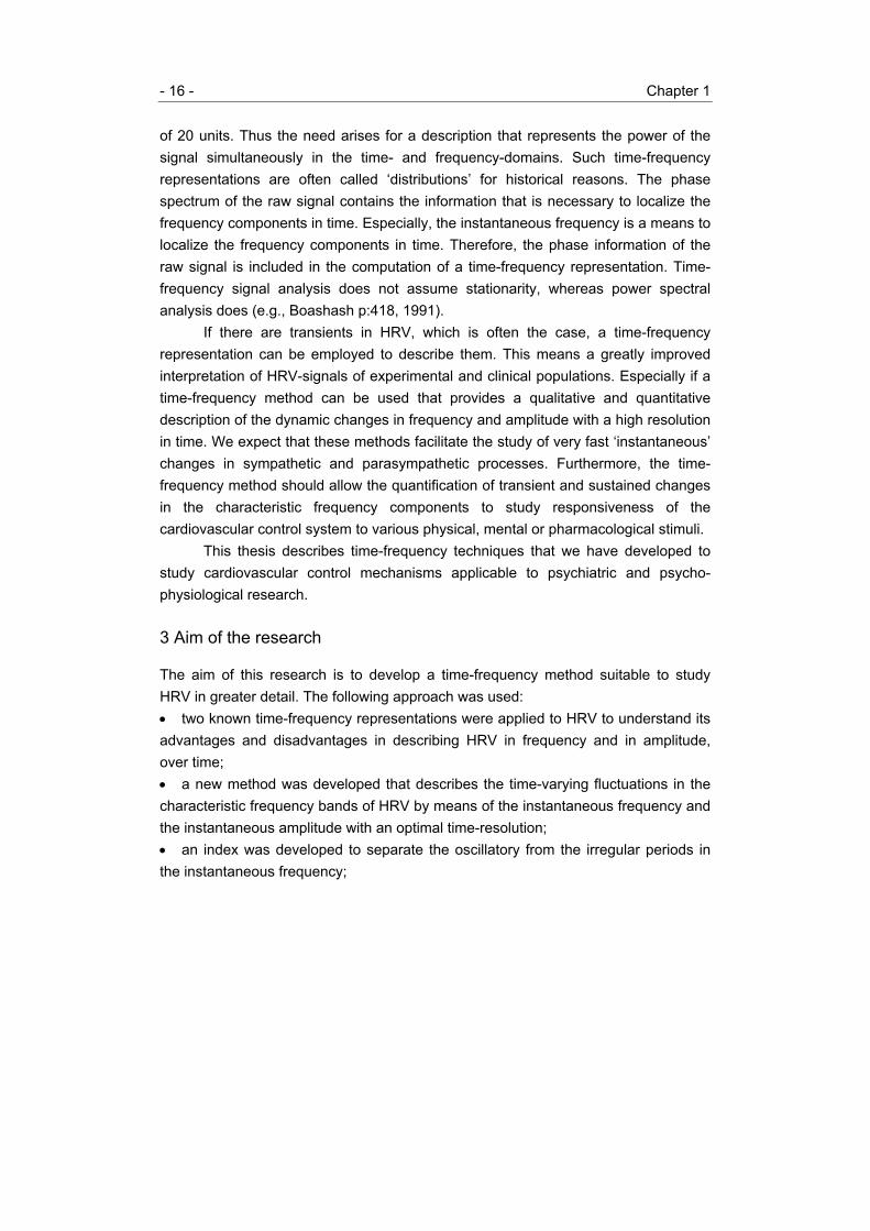
If there are transients in HRV, which is often the case, a time-frequencyrepresentation can be employed to describe them. This means a greatly improvedinterpretation of HRV-signals of experimental and clinical populations. Especially if atime-frequency method can be used that provides a qualitative and quantitativedescription of the dynamic changes in frequency and amplitude with a high resolutionin time. We expect that these methods facilitate the study of very fast ‘instantaneous’changes in sympathetic and parasympathetic processes. Furthermore, the time-frequency method should allow the quantification of transient and sustained changesin the characteristic frequency components to study responsiveness of thecardiovascular control system to various physical, mental or pharmacological stimuli.
This thesis describes time-frequency techniques that we have developed tostudy cardiovascular control mechanisms applicable to psychiatric and psycho-physiological research.
3 Aim of the research
The aim of this research is to develop a time-frequency method suitable to studyHRV in greater detail. The following approach was used:• two known time-frequency representations were applied to HRV to understand itsadvantages and disadvantages in describing HRV in frequency and in amplitude,over time;• a new method was developed that describes the time-varying fluctuations in thecharacteristic frequency bands of HRV by means of the instantaneous frequency andthe instantaneous amplitude with an optimal time-resolution;• an index was developed to separate the oscillatory from the irregular periods inthe instantaneous frequency;
Introduction - 17 -
• from the instantaneous amplitude and frequency, we derived summarizingparameters which we applied to describe the changes in the instantaneous amplitudeand frequency over time for the oscillatory and irregular periods separately.
4 Outline of the thesis
Chapter 2 presents an overview of existing techniques to analyze HRV in the time-domain, the frequency-domain, and the time-frequency domain.
Chapter 3 describes methods for frequency analysis on non-equidistantlysampled HRV-signals. It paves the way for the application of time-frequencytechniques to such signals.
Chapter 4 summarizes the results of experiments using the frequency-domaintechniques of chapter 3. The spectral estimates of heart rate and blood pressurevariability were computed. They described changes in sympathetic and para-sympathetic cardiovascular processes as a result of pharmacological challenge tests(clonidine, lorazepam, epinephrine, norepinephrine) in healthy volunteers. They alsodescribed the effects of antidepressant treatment (imipramine, mirtazapine) on theautonomic cardiovascular control processes of depressed patients.
Chapters 5 and 6 demonstrate the applicability of two known time-frequencyrepresentations. This was done by visualizing and analyzing the instantaneousspectral changes in HRV, blood pressure, and respiratory signals. These signalswere obtained from healthy subjects, patients with pure autonomic failure, anddepressed patients. The signals were measured during supine rest, mental stress,and orthostatic challenge.
Chapter 7 presents a new method to describe the time-varying properties ofHRV by the instantaneous amplitude and frequency. A measure of the instantaneousbandwidth, the instantaneous bandwidth coefficient, was developed to separateirregular and oscillatory periods in the instantaneous frequency.
In chapter 8, the instantaneous frequency was compared to three othermethods: the discrete time-frequency transform, the circular mean direction of thetime-slices of the Wigner-Ville distribution, and the central finite difference of theinstantaneous phase.
In chapter 9, our new method was applied to HRV-data obtained from healthysubjects during supine rest and orthostatic challenge. A number of summarizingparameters were defined to quantitatively describe changes in the instantaneousamplitude and frequency over time.

- 18 - Chapter 1
Chapter 10 summarizes the advantages of our time-frequency method inconjunction with its relevance for clinical research.
References
Akselrod S, Gordon D, Ubel FA, Shannon DC, and Cohen RJ. Power spectrumanalysis of heart rate fluctuation: a quantitative probe of beat-to-beatcardiovascular control. Science 213:220-222, 1981.
Bendat JS and Piersol AG. Random Data, Analysis and Measurements Procedures,2nd edition. New York: John Wiley and Sons, Inc., 1986.
Bigger JT, Fleiss JL, Rolnitzky LM, Steinman RC. The ability of several short-termmeasures of RR variability to predict mortality after myocardial infarction.Circulation 88: 927-934, 1993.
Black DW, Warrack G, and Winokur G. Excess mortality among psychiatric patients.The Iowa record-linkage study. JAMA 253:58-61, 1985.
Boashash B. Time-frequency signal analysis. In: Advances in Spectrum Analysis andArray Processing, Vol. 1. S. Haykin, Ed. Englewood Cliffs, NJ: Prentice Hall,pp:418-517, 1991.
Cohen L. Time-Frequency Analysis. Englewood Cliffs, NJ: Prentice Hall Inc, 1995.Dalack GW and Roose SP. Perspectives on the relationship between cardiovascular
disease and affective disorder. J Clin Psychiatry 51(suppl): 4-9, discussion 10-1,1990.
Hayward C. Psychiatric illness and cardiovascular disease risk. Epidemiol Rev17:129-138, 1995.
Hyndman BW, Kitney RI, and Sayers BMcA. Spontaneous rhythms in psysiologicalcontrol systems. Nature 233:339-341, 1971.
Kamath MV and Fallen EL. Power spectral analysis of heart rate variability: anoninvasive signature of cardiac autonomic function. Crit Rev in Biomed Eng21(3):245-311, 1993.
Kikuya M, Hozawa A, Ohokubo T, Tsuji I, Michimata M, Matsubara M, Ota M, NagaiK, Araki T, Satoh H, Ito S, Hisamichi S, and Imai Y. Prognostic significance ofblood pressure and heart rate variabilities: the Ohasama study. Hypertension36:901-906, 2000.
Kitney RI. Entrainment of the human RR interval by thermal stimuli. J Physiol252:37P-38P, 1975.
Kobayashi M and Musha T. 1/f Fluctuations of heartbeat period. IEEE Trans BiomedEng BME-29:456-457, 1982.

Introduction - 19 -
Malliani A, Pagani M, Lombardi F, and Cerutti S. Cardiovascular neural regulationexplored in the frequency domain. Circulation 84:482-492, 1991.
Malzberg B. Mortality among patient with involution melancholia. Am J Psychiatry93:1231-1238, 1937.
Miyawaki E, Salzman C. Autonomic nervous system tests in psychiatry: implicationsand potential uses of heart rate variability. Integr Psychiatry 7:21-28, 1991.
Parati G, Saul JP, di Rienzo M, and Mancia G. Spectral analysis of blood pressureand heart rate variability in evaluating cardiovascular regulation. A criticalappraisal. Hypertension 25:1276-1286, 1995.
Di Rienzi M, Parati G, Castiglioni P, Mancia G, and Pedotti A. The wide band spectralanalysis: a new insight into modulation of blood pressure, heart rate andbaroreflex sensitivity. In: Computer Analysis of Cardiovascular Signals. DiRienzi M, Mancia G, Parati G, Pedotti A, and Zanchetti A (eds). Amsterdam:IOS Press pp:67-74, 1995.
Sayers BMcA. Analysis of heart rate variability. Ergonomics 16:17-32, 1973.Singh JP, Larson LG, Tsuji H, Evans JC, O'Donnell CJ, and Levy D. Reduced heart
rate variability and new-onset hypertension: insights into pathogenesis ofhypertension: the Framingham Heart Study. Hypertension 32:293-297, 1998.
Steeghs P. Local power spectra and seismic interpretation (Ph.D. Thesis). Delft: DelftUniversity of Technology, 1997.
Task force of the European society of cardiology and the North American society ofpacing and electrophysiology. Heart rate variability – standards ofmeasurement, physiological interpretation, and clinical use. Eur Heart J 17:354-381, 1996.
Ten Voorde BJ. Modeling the baroreflex: a systems analysis approach (Ph.D.Thesis). Amsterdam: Free University Amsterdam, 1992.
Tsuji H, Larson MG, Venditti FJ Jr, Manders ES, Evans JC, Feldman CL, and Levy D.Impact of reduced heart rate variability on risk for cardiac events. TheFramingham Heart Study. Circulation 94:2850-2855, 1996.
Tulen JHM, Bruijn JA, De Man KJ, Pepplinkhuizen L, Van den Meiracker AH, andMan in 't Veld AJ. Cardiovascular variability in major depressive disorder andeffects of imipramine or mirtazapine (org 3770). Journal of ClinicalPsychopharmacology 16:135-145, 1996.
Van Roon AM. Short-term cardiovascular effects of mental tasks – physiology,experiments and computer simulations (Ph.D. Thesis). Groningen: University ofGroningen, 1998.

- 20 - Chapter 1
Wesseling KH and Settels JJ. Baromodulation explains short-term blood pressurevariability. In: Psychophysiology of Cardiovascular Control. Orlebeke JF, MulderG, Van Doornen LJP (eds). New York & London: Plenum Press pp:69-97, 1985.
Yeragani VK, Pohl R, Balon R, Ramesh C, Glitz D, Jung I, Sherwood P. Heart ratevariability in patients with major depression. Psychiatry Research 37:35-46,1991.

CHAPTER 2HEART RATE VARIABILITY AND ITS ANALYSIS


Heart rate variability - 23 -
This chapter introduces the concept of heart rate variability and defines variousrepresentations of heart rate variability that can be used for various analysistechniques, such as spectral analysis. Spectral analysis and time-frequency analysisare explained. The chapter ends with a section on the instantaneous amplitude andfrequency of narrow frequency bands.
1 Heart rate and heart rate variability
The human heart contracts and relaxes rhythmically, with each contraction pumpingblood from the veins to the arteries. The complete cycle of contraction and relaxationis called a heartbeat or cardiac cycle. Each heartbeat is initiated by an electricimpulse, called an action potential. The action potentials are generated in thesinoatrial node of the heart, which is a specialized group of cells in the right atrial wallof the heart (e.g., Guyton et al., 1996). Contraction and relaxation of the heart arepreceded by electrical phenomena that can be measured on the skin by means of anelectrocardiogram (ECG). This complex of electric phenomena or waves in onecardiac cycle is depicted in figure 1 (e.g, Guyton et al., 1996).
Heart rate (HR) is the occurrence rate of the cardiac cycle per unit time,conventionally, per minute (e.g., Rompelman, 1980; Guyton et al., 1996). Heart rateis also called heart rhythm. To determine this rate, it should be sufficient to measurethe time-intervals between adjacent sinoatrial action potentials. However, these arenot detectable in the ECG. The nearest to this action potential is the P-wave. Thusthe period of time between two adjacent P-waves could be measured, but the onsetof a P-wave is not sharply defined. In general, the sharp R-waves of the QRS-
Cardiac Cycle
0 0.2 0.4 0.6 0.8 1time (s)
R
P
Q S
T
Figure 1. An example of one cardiac cycle or heart beat.

- 24 - Chapter 2
complex are easier to detect and the period between two consecutive R-waves iscalled the R-R interval or interbeat interval (IBI). The interbeat intervals determine inpractice the heart rate. It should be noted that the P-R interval shows slightfluctuations. This causes small differences between the heart rate measured from theonset of P- or from the R-waves. Since this thesis deals with small fluctuations inheart rate, the effect must be mentioned, but it is almost always ignored in practice(Rompelman, 1980).
The generation of action potentials is a rhythmic process. Repetitive self-induced discharges cause potential depolarizations in the cell membranes of thesinoatrial node and thereby firing action potentials. This results in a fairly constantheart rhythm (e.g., Guyton et al., 1996). However, the heart rhythm is modulated bythe autonomic nervous system. Varying sympathetic and parasympathetic nervousactivity modulates the firing rate of the sinoatrial node. Therefore, the duration of thecardiac cycle varies. These variations in duration are called beat-to-beat fluctuations(of the cardiac cycles). The beat-to-beat fluctuations in heart rate are called heart ratevariability (HRV) (Task Force p:354, 1996). HRV may be studied in the time-domain,the frequency-domain, or in the time-frequency domain. An HRV-representation isthe beat-to-beat information derived from the ECG that is of interest for HRV-analysisand ordered in such a way that it is accessible to the analysis techniques (De Boerpp:20,28, 1985; De Boer et al., 1985) and can be related to other physiologicalprocesses (Rompelman p:124, 1987; Mulder p:5, 1988). This information may consistof a listing of interbeat intervals derived from the ECG or a listing of inverses ofinterbeat intervals, called instantaneous heart rates. The interbeat intervals areexpressed in s, the instantaneous heart rates are expressed in s-1, or moreconventionally in beats per minute.
2 Various HRV-representations
When we state that the oscillations in the heart rate are called heart rate variabilitythere are still several ways in which this can be described and displayed. A first andobvious way is to make a list of the successive interbeat interval values orinstantaneous heart rate values that are measured by detecting the R-waves from theECG. Since these values occur with increasing time, the various interbeat interval orinstantaneous heart rate values in the list may be ordered by means of an increasingindex. An indexed list of interbeat intervals is called an interbeat interval timeseries. An indexed list of instantaneous heart rates is called a heart rate timeseries. The index may be a number starting from 1 and increasing with 1: (1,2,3,4...).

Heart rate variability - 25 -
When the list is plotted on a horizontal axis the heart rate values are plotted atregular horizontal distances. Often the regular horizontal increment is taken as theaverage interbeat interval in seconds. This transforms the horizontal axis to a timeaxis. In this case the indices are equidistantly spaced and the list is called anequidistant time series.
The index may also be the R-wave occurrence time. In that case the valuesare placed at the instant of detection of the second R-wave of the R-wave pairbetween which the interbeat interval or the instantaneous heart rate value wasmeasured. When we plot a time series indexed by R-wave occurrence time, thevalues of the list are now plotted at irregular horizontal intervals. This is because theheart rate in general is not constant. The horizontal axis is now naturally a time axisand the list is called a non-equidistant time series.
This leads to the definition of four different HRV-representations (see figures 2and 3):• The interbeat interval series is an equidistant interbeat interval time series.• The heart rate series is an equidistant heart rate time series.• The interbeat interval function is a non-equidistant interbeat interval time series.• The instantaneous heart rate function is a non-equidistant heart rate timeseries.These representations were studied by various authors, for instance, Rompelman etal. (1977), De Boer (pp:29-32,49, 1985), and Janssen et al. (1993).
There are still more HRV-representations. Another representation of heart ratevariability is obtained by replacing the R-wave by a narrow positive spike of constantunit impulse generated at the instant that the R-wave is detected (see figure 4). Ifeach R-wave is called an event, the series of events is called an R-wave event seriesor cardiac event series (CES) (e.g., Hyndman et al., 1975a; 1975b; Rompelman etal., 1977; 1985). It is further possible to multiply each constant spike by the value ofthe interbeat interval obtained at that instant, multiplied with the duration of thepreceding R-R interval. The result is called the interbeat interval event series. Theequivalent for the instantaneous heart rate is called the heart rate event series (e.g.,Mulder, 1988; Van Steenis, 1994).

- 26 - Chapter 2
t0 t4t3t2t1
IBI1 IBI4IBI3IBI2
A
1 2 43IBI 1 2 3 4IHR
CB
t0 t1 t2 t3 t4
IHR2 IHR4
IHR3
IHR1
E
IBI3
t0 t1 t2 t3 t4
IBI1
IBI4IBI2
D
Figure 2. HRV-representations (e.g., Rompelman et al., 1977; De Boer p:49, 1985;Janssen et al., 1993). Abbreviations: IBI = interbeat interval; IHR = instantaneousheart rate.A: ECG with R-waves at it , and interbeat intervals 1IBIi i it t −= − , the instantaneousheart rates IHR i are the inverses of IBIi ;B: interbeat interval series: the IBIi are indexed by number i ;C: heart rate series: the IHR i are indexed by number i ;D: interbeat interval function: the IBIi are placed as a function of time it ;E: instantaneous heart rate function: the IHR i are placed as a function of time it .

Heart rate variability - 27 -S
pect
ral a
naly
sis
(2.3
)H
RV
-rep
rese
ntat
ions
(2.2
)
EC
G
EC
GR
-wav
ede
tect
ion
(2.1
)
plac
e sp
ikes
at
R-w
ave
even
ts(2
.2)
sam
ple
IBIs
or
IHR
s(2
.1)
form
atio
n of
time
serie
s(2
.2)
inte
rbea
t int
erva
lse
ries
(fig
.2B
)
inte
rval
spec
trum
hear
t rat
esp
ectr
um
inst
. hea
rt r
ate
func
tion
(fig
.2E
)
inte
rbea
t int
erva
lfu
nctio
n(f
ig.2
D)
hear
t rat
ese
ries
(fig
.2C
)
non-
equi
dist
ant
time
serie
s
equi
dist
ant
time
serie
s
LPF
CE
S(f
ig.4
)
hear
t rat
eev
ent s
erie
s
inte
rbea
t int
erva
lev
ent s
erie
s
inst
.hea
rt r
ate
spec
trum
(ch.
3)
inst
.inte
rval
spec
trum
(ch.
3)
card
iac
even
t ser
ies
spec
trum
of c
ount
s(c
h.3)
sam
ple
IBIs
or
IHR
s(2
.1)
even
t ser
ies
low
-pas
s fil
terin
g(2
.2)
time-
freq
uenc
yan
alys
is(2
.4-2
.5;c
h.5-
9)
spec
trum
spec
trum
Figure 3. Summary of the sections 2 and 3. Abbreviations: ECG = electro-cardiogram; IBI = interbeat interval; IHR = instantaneous heart rate; LPFCES =low-pass filtered cardiac event series; inst. = instantaneous. The numbers refer tosections and figures of chapter 2.

- 28 - Chapter 2
The unit spikes of the CES are placed at irregular distances. An equidistanttime-series may be obtained by filtering the CES with some low-pass filter andsampling this signal. Often a cutoff frequency of 0.5 Hz is used. This result is calledthe low-pass filtered cardiac event series (see figure 3) (e.g., Hyndman et al.,1975a; 1975b; Rompelman et al., 1977; French et al., 1971; Peterka et al., 1978). Weused a zero-phase low-pass finite impulse response (FIR)-filter (Oppenheim et al.,1999). This filter is non-causal. The pass-band is the frequency interval [0, 0.5]. The-6 dB point is at 0.5 Hz. The transition band between 0.4863 Hz and 0.5137 Hz is‘cos2-shaped’ (see figure 5). The low-pass filtered cardiac event series is comparablewith heart rate, because whenever the heart rate is higher, there are more spikeswith smaller intervals between them, and consequently, the filter output will be higher(see figure 4). To use this signal digitally it must be sampled, in our case with asample frequency of 4 Hz.
0 5 10 15 20 25time (s)
Hz
ECG
CES
LPFCES
1.5
0.5
Figure 4. From ECG to LPFCES: the R-waves in the ECG (upper graph) aredetected and represented by spikes placed at the R-wave occurrence times. Thisconstitutes a function of time, called the cardiac event series (CES, middle graph).The CES is filtered with a zero-phase low-pass FIR-filter with cutoff frequency of0.5 Hz. This results in a low-pass filtered cardiac event series (LPFCES) (e.g., DeBoer p:32, 1985).

Heart rate variability - 29 -
Low-pass filter
-0.25
0
0.25
0.5
0.75
1
1.25
0.47 0.48 0.49 0.5 0.51 0.52 0.53frequency (Hz)
ampl
itude
(a.u
.)
A
Low-pass filter
-210-180-150-120-90-60-30
030
0 0.5 1 1.5 2frequency (Hz)
Am
plitu
de (d
B)
B
Impulse Response
-0.1
0
0.1
0.2
0.3
-10 -5 0 5 10time (s)
a.u.
C
Figure 5. To obtain a low-pass filtered cardiac event series, the cardiac eventseries is filtered with a zero-phase low-pass FIR-filter. The –6 dB point is at 0.5Hz. The pass-band ranges from 0 to 0.5 Hz. The transition band ranges from0.4863 to 0.5137 Hz and has a cos2-shaped slope. Figure A shows the transitionband. Figure B shows the amplitude of the frequency response in dB. Figure Cshows the truncated impulse response of this filter. The total duration is 183 s.Note that this FIR-filter is non-causal.

- 30 - Chapter 2
Although we now already have eight representations, all with slightly differentproperties, several more can be defined and have been in use. This makes HRV-studies confusing for the uninitiated. In the study of time-frequency analysis of HRV(chapters 7,8, and 9), we limited ourselves to the use of the low-pass filtered cardiacevent series, based on its slightly superior properties for our purpose (e.g.,Rompelman, 1980; Rompelman et al., 1977; Mulder pp:8,51-52, 1988). However, theuse of any other representation may serve just as well when the fluctuations aresmall with respect to the average heart rate.
3 Spectral analysis of heart rate variability
In the previous sections we have described how heart rate (and interbeat interval)can be derived from the ECG and how a number of slightly different representationsof heart rate variability came into use. When looking at abritrary HRV-signals itappears that often both noise-like and sinusoidal-like variability components arepresent (see figures 2A and 3A of chapter 1). The overall picture may be quiteconfusing and at times when the sinusoidal oscillations are small in amplitude theymay even become invisible in the noise. However, these ‘invisible’ oscillations maybecome ‘visible’ by means of spectral analysis. What is spectral analysis?
Let us take an interval of heart rate variability of, say, 100 s. To this interval weapply a discrete Fourier transform and we obtain the same signal as before but in yetanother form or representation. The result of this Fourier transform is a list of all thefrequencies, from the fundamental harmonic (here 0.01 Hz) up, that occur in theheart rate variability with their amplitude and their phase in the form of a complexnumber. This means that to each frequency in the list, a complex number is assignedby the transform. This is called a spectrum. In the spectrum we can usually observethe noisy component separated from the sinusoidal component since they usuallydiffer in frequency. The noise is usually concentrated towards the fundamentalharmonics (those from 0.01 Hz up), whereas the sinusoidal components arepredominant near 0.1 Hz and near 0.3 Hz (see figures 2B and 3B of chapter 1). Thuswe have now obtained a much clearer picture of the sinusoids in the heart ratevariability signal.
There is nothing special about the spectrum. Given the spectrum, the originaldata can be reconstructed by means of another discrete Fourier transform and soforth and so on. The absolute values of the complex numbers of the spectrum areoften squared. The result is called the power spectrum (or power spectral densityfunction). Because of the squaring action the phase is lost and the high amplitudes
Heart rate variability - 31 -
are emphasized with respect to the smaller amplitudes. A further effect is that weclearly see the amplitude of the sinusoid of a particular frequency but from thespectrum alone we do not know at which point in time this frequency occurred. Infact, the spectrum gives an average of the amplitude of an oscillation at a certainfrequency over the entire 100 s duration of the signal. We gain some, we loose some.
Spectral analysis of HRV-representations signals was used at an early stageby Penaz et al. (1968), and by Sayers (1973), to name just two pioneers. Spectralanalysis can be applied to each of the HRV-representations of section 2. Somespectra have names. We just mention these names. The power spectral densityfunction• of an interbeat interval series is called the interval spectrum;• of a heart rate series is called the heart rate spectrum;• of a CES is called the spectrum of counts;• of an interbeat interval event series is called the instantaneous intervalspectrum;• of an heart rate event series is called the instantaneous heart rate spectrum.This is shown in figure 3. The different techniques of spectral analysis were studiedby Luczak et al. (1973), Hyndman et al. (1975a; 1975b), Mohn (1976), Rompelman etal. (1982), Rompelman (1985; 1987), Pomeranz et al. (1985), De Boer (ch.3, 1985),Mulder (pp:51-57, 1988), Van Steenis et al. (1994), Parati et al. (1995), and manymore.
Two examples of spectra of counts are shown in figures 2B and 3B of chapter1. Mulder (1988) developed a computer program, called CARSPAN, to compute thepower spectral density function of a CES and of an interbeat interval event series.
4 Time-frequency analysis of heart rate variability
Let us return to the 100 s interval of HRV (section 3). Suppose we sampled theinterval with a sample frequency of 1 Hz. Then the interval of 100 s delivers 100 data-points. The time-resolution is 1 s, and the frequency range of the power spectrum ofthis interval ranges from 0 until 0.5 Hz in steps of 0.01 Hz. Suppose now thereappears a sinusoid with a frequency of 0.2 Hz at the 20th second and disappears atthe 40th second. Then we observe a peak in the power spectrum at 0.2 Hz. However,from the spectrum alone we do not know at which points in time this sinusoidoccurred. Suppose, for the sake of clarification, that at each second of the time-interval, we are able to compute a list of frequencies that occur at that instant,together with their amplitude and their phase. Of each list we can compute the power

- 32 - Chapter 2
spectrum. This results in a list of 100 power spectra: one for each instant in the time-interval, i.e., they are computed instantaneously. We call these spectra:instantaneous power spectra. When we plot this list of instantaneous power spectra,ordered according to increasing time, we see that there appears a frequencycomponent of 0.2 Hz in the 20th second. It stays in the successive spectra until the39th second, after which the sinusoid disappears. Furthermore, if the amplitude of thesinusoid varies in time, the heights of the peaks in the instantaneous spectra variescorrespondingly. Such a list of instantaneous power spectra is called a time-frequency representation: it represents the power of a signal simultaneously in timeand frequency. The strength of a time-frequency representation is that it visualizestime-varying frequency components in a signal when they come and go. In the nextsection we discuss some forms of time-frequency representations that are used inthe study of HRV. In the chapters 5 and 6 we applied two time-frequencyrepresentations to HRV.
5 The instantaneous amplitude and frequency of narrow frequencybands
In the example of section 3 we observed 2 frequency peaks, one near 0.1 Hz andone near 0.3 Hz. However, in general these peaks are not narrow, but they have awidth or spread (see figures 2B and 3B of chapter 1). As peaks they do not standalone, but protrude above a general background. Take, for example, the peak near0.1 Hz. How was this peak brought about? Is it the result of a sinusoid of which thefrequency is fluctuating in time? Or is it the result of a sinusoid of which the amplitudeis fluctuating in time? Maybe it is a combination of both? With a time-frequencyrepresentation this complex component can be visualized. However, we want to go alittle further and analyze, for example, this component near 0.1 Hz quantitatively. Inthe instantaneous spectra (see section 4) of the time-frequency representation wesee this component changing in amplitude, in frequency location, and in spread, withincreasing time. The next step is that we want to compute these parameters at eachindependent instant of the time-interval. If we manage to do this, the amplitude iscalled the instantaneous amplitude, the frequency is called the instantaneousfrequency, and the spread is called the instantaneous bandwidth of this component inthe signal.
What are independent instants in practice? Suppose we filter the signal ofsection 3 with a low-pass filter. After the low-pass filter, the original samples of thesignal become dependent because the signal does no longer change as quickly and

Heart rate variability - 33 -
adjacent samples become linked or correlated. We say that the signal is over-sampled. Suppose each four adjacent points are dependent and every fifth instant isindependent. The 1st point, the 5th point, the 9th point, and so on, are independentinstances. Adjacent disjoint time-intervals of 4 s are likewise independent. Supposewe can compute a value of a signal property in these intervals: one value for eachinterval. Then we can say that the resulting adjacent values in time are placed atindependent instances. This means that these properties are instantaneousproperties. Otherwise, computations over a shorter time interval yield adjacentlydependent points in time; if computed over a longer time interval, the values of theproperties will be averaged. We now define that a signal property, which can becomputed within the time-resolution of the signal, is an instantaneous property (seechapter 7).
The next step in the time-frequency analysis of HRV is the analysis of thecharacteristic frequency bands of HRV by means of the instantaneous amplitude,frequency, and a measure of the instantaneous bandwidth. After filtering the HRV-signal with a filter corresponding with one of the characteristic frequency bands, wecan determine the time-resolution of the filtered signal and compute theseparameters instantaneously. This is described in chapter 7, 8, and 9.
References
De Boer RW. Beat-to-beat blood-pressure fluctuations and heart-rate variability inman: physiological relationships, analysis techniques and a simple model (Ph.D.Thesis). Amsterdam: University of Amsterdam, 1985.
De Boer RW, Karemaker JM, and Strackee J. Description of heart-rate variabilitydata in accordance with a physiological model for the genesis of heart beats.Psychophysiology 22:147-155, 1985.
French AS and Holden AV. Alias-free sampling of neuronal spike trains. Kybernetic5:165-171, 1971.
Guyton AC and Hall JE. Textbook of Medical Physiology. Ninth Edition. Philadelphia,PA: Saunders, 1996.
Hyndman BW and Mohn RK. A model of the cardiac pacemaker and its use indecoding the information content of cardiac intervals. Automedica 1:239-252,1975a.
Hyndman BW and Gregory JR. Spectral analysis of sinus arrhythmia during mentalloading. Ergonomics 18:255-270, 1975b.

- 34 - Chapter 2
Janssen MJA, Swenne CA, De Bie J, Rompelman O, and Van Bemmel JH. Methodsin heart rate variability analysis: which tachogram should we choose? ComputerMethods and Programs in Biomedicine 41:1-8, 1993.
Luczak H and Laurig W. An analysis of heart rate variability. Ergonomics 16:85-97,1973.
Mohn RK. Suggestions for the harmonic analysis of point process data. ComputBiomed Res 9:521-530, 1976.
Mulder LJM. Assessment of cardiovascular reactivity by means of spectral analysis(Ph.D. Thesis). Groningen: University of Groningen, 1988.
Oppenheim AV, Schafer RW, and Buck JR: Discrete-Time Signal Processing, 2nd
edition. Englewood Cliffs, NJ: Prentice Hall, 1999.Parati G, Saul JP, di Rienzo M, and Mancia G. Spectral analysis of blood pressure
and heart rate variability in evaluating cardiovascular regulation. A criticalappraisal. Hypertension 25:1276-1286, 1995.
Penaz J, Roukens J, and Vanderwaal HJ. Spectral analysis of some spontaneousrhythms in the circulation. In: Biokybernetik, Drische H and Tiedt N (eds).Leipzig: K.Marx Universitat pp:233-236, 1968.
Peterka RJ, Sanderson AC, and O'Leary DP. Practical considerations in theimplementation of the French-Holden algorithm for sampling neuronal spiketrains. IEEE Trans Biomed Eng BME-25:192-195, 1978.
Pomeranz B, MacAulay RJB, Caudill MA, Kutz I, Adam D, Gordon D, Kilborn KM,Barger AC, Shannon DC, Cohen RJ, and Benson H. Assessment of autonomicfunction in humans by heart rate spectral analysis. Am J Physiol 248:H151-H153, 1985.
Rompelman O. The assessment of fluctuations in heart-rate. In: The study of heart-rate variability. Kitney RI, Rompelman O (eds). Oxford: Clarendon Press pp:59-77, 1980.
Rompelman O. Spectral analysis of heart-rate variability. In: Psychophysiology ofCardiovascular Control. Orlebeke JF, Mulder G, Van Doornen LJP (eds). NewYork & London: Plenum Press pp:315-331, 1985.
Rompelman O. Hartritmevariabiliteit – meting, verwerking, interpretatie (Ph.D.Thesis). Delft: Delft University of Technology, 1987.
Rompelman O, Coenen AJRM, and Kitney RI. Measurement of heart-rate variability:part 1 – comperative study of heart-rate variability analysis methods. Med & BiolEng & Comput 15:233-239, 1977.

Heart rate variability - 35 -
Rompelman O, Snijder JBIM, and van Spronsen CJ. The measurement of heart ratevariability spectra with the help of a personal computer. IEEE Trans BiomedEng BME-29:503-510, 1982.
Sayers BMcA. Analysis of heart rate variability. Ergonomics 16:17-32, 1973.Task Force of the European society of cardiology and the North American society of
pacing and electrophysiology. Heart rate variability – standards ofmeasurement, physiological interpretation, and clinical use. Eur Heart J 17:354-381, 1996.
Van Steenis HG, Tulen JHM, and Mulder LJM. Heart rate variability spectra based onnon-equidistant sampling: the spectrum of counts and the instantaneous heartrate spectrum. Medical Engineering and Physics 16:355-362, 1994.

- 36 - Chapter 2

CHAPTER 3HEART RATE VARIABILITY SPECTRA BASED ON NON-EQUIDISTANT SAMPLING: THE SPECTRUM OF COUNTSAND THE INSTANTANEOUS HEART RATE SPECTRUM
Medical Engineering and Physics 16:355-362, 1994
H.G. van Steenis1,3, J.H.M. Tulen2,3, L.J.M. Mulder4
1Department of Clinical Neurophysiology, University Hospital Rotterdam Dijkzigt2Department of Psychiatry, Erasmus University Rotterdam3Section Pathophysiology of Behaviour, Erasmus University Rotterdam4Experimental and Occupational Psychology, University of Groningen


Heart rate variability spectra - 39 -
This paper compares two methods to estimate heart rate variability spectra, i.e., thespectrum of counts and the instantaneous heart rate spectrum. Contrary to Fouriertechniques based on equidistant sampling of the interbeat intervals, the spectrum ofcounts and the instantaneous heart rate spectrum are based on non-equidistantsampling: the values are determined at R-wave occurrence times. A consequence ofthe non-equidistant occurrence of the R-peaks in a heart rate signal is theappearance of the sidebands of the harmonic components of the mean heart rate inthe spectra. These sidebands contaminate the signal components in the spectrum.The sideband distortion in the instantaneous heart rate spectrum was found to besmaller than in the spectrum of counts. Simulations using the IPFM-model weremade to quantify this difference. On basis of these simulations, sideband distortionappeared to be dependent on the mean heart rate, the modulation depth and themodulation frequency.
1 Introduction
Spectral analysis of beat-to-beat fluctuations in heart rate can be used as aquantitative and non-invasive technique for the study of the functioning of short-termcardiovascular control. Fluctuations in heart rate are believed to contain informationrelated to sympathetic and parasympathetic activity within the cardiovascular controlsystem (Hyndman et al., 1971; Sayers, 1973; Akselrod et al., 1981; 1985).From the electrocardiogram (ECG), the R-wave occurrence times are determinedand the interval lengths (interbeat interval: IBI) between consecutive R-waves, aswell as the heart rate, are measured. It has been shown that the variations in theinterbeat interval time series do not produce a random pattern (Sayers, 1980), butshow certain frequency-specific properties (Sayers, 1973; Akselrod et al., 1981).Therefore, spectral analysis is an important method to describe frequency-dependentaspects of heart rate variability. The following frequency bands are recognized in theheart rate variability spectrum (Sayers, 1973; Mulder, 1988):a) variations related to temperature regulation of the body (0.02–0.06 Hz, lowfrequency band);b) variations related to intrinsic characteristics of the blood pressure control system(0.06–0.14 Hz, mid frequency band) andc) variations mainly related to respiratory activity (0.14–0.50 Hz, high frequencyband).
Several techniques have been developed to estimate heart rate variabilityspectra. Baselli et al. (1985; 1986) used a parametric method for autoregressive
- 40 - Chapter 3
spectral analysis of heart rate time series. This method calculates a number ofparameters which are used to describe the spectrum.
Non-parametric methods in general make use of a discrete Fourier transform(Bendat and Piersol, 1986). Some of these methods are based on equidistantsampling of the interbeat interval lengths (Sayers, 1973; 1980; Mohn, 1976; De Boeret al., 1984), or inverse interval lengths (Mohn, 1976; De Boer et al., 1984). Theintervals (figure 1a), or inverse interval lengths (figure 1b), are placed equidistantly asa function of interval number. Spectra can then be calculated using a fast Fouriertransform (FFT) (Cooley and Tukey, 1965). This is a fast way to calculate thespectra, but the disadvantages are that the number of data points has to be a powerof two and the spectra are functions of ‘cycles per beat’ instead of ‘cycles per second’(De Boer et al., 1984). Such an approach may become a problem when timerelations between signals have to be studied (such as between heart rate andrespiration), because this method may introduce relative time shifts between timeseries which are not constant as a function of time.
Other methods are based on interpolation of non-equidistantly sampledinterbeat intervals. Firstly, the intervals are placed non-equidistantly at R-waveoccurrence times (figure 1c) (Luczak and Laurig, 1973), or the inverse intervallengths are placed non-equidistantly at the R-wave occurrence times (figure 1d)(Womack, 1971). Then the time series is interpolated and the resulting signal issampled equidistantly. From these sampled data points, the spectrum can beestimated using a fast Fourier transform. The disadvantage is that a zero orderinterpolation often results in a discontinuous signal and a first order interpolation alsoresults in unwanted effects in the spectrum (Luczak and Laurig, 1973; De Boer et al.,1984). Berger et al. (1986) used a series of interpolated inverse intervals.
In this paper we evaluate two other methods, based on non-equidistantsampling, to estimate the heart rate variability spectrum. These methods are:1) the spectrum of counts (SOC) (Rompelman, 1985): at each R-wave occurrencetime, a delta function of unit area is placed (figure 1e); this sequence of deltafunctions is transformed with a discrete Fourier transform in order to estimate thepower spectrum;2) the instantaneous heart rate spectrum (IHRS): at each R-wave occurrence time,the interbeat interval length is measured. A delta function of unit area, but with weight(or amplitude) equal to the inverse interval length, is placed at the R-waveoccurrence time (figure 1d); a discrete Fourier transform is applied to estimate thepower spectrum of this time series. This IHRS is based on a method of Mulder(1988).

Heart rate variability spectra - 41 -
1 N432
1 2 3 4 N
t1
I1
tNt4t3t2
1/I1
IN
I4
I3I2
1/IN1/I4
1/I3
1/I2
I1
I2
I3
I4
IN
a
c
b
tN
t4t3t2t1
1/I1 1/IN1/I4
1/I3
1/I2
tN
t4t3t2t1 tN
t4t3t2t1
x1I1
x4I4x3I3
x2I2 xNIN
f
e
d
Figure 1: Methods to sample a heart rate variability signal.a) A series of interbeat interval lengths as function of interval number, theintervals are sampled equidistantly.b) A series of inverse interval lengths as function of interval number, the intervalsare sampled equidistantly.c) A series of interbeat interval lengths as function of time, the intervals aresampled non-equidistantly at R-wave occurrence times.d) A series of inverse interval lengths as function of time, the intervals aresampled non-equidistantly at R-wave occurrence times.e) A series of delta pulses as a function of time, the pulses are placed non-equidistantly at R-wave occurrence times.f) A series of delta pulses as a function of time, the pulses are placed non-equidistantly at R-wave occurrence times and have weights equal to the sample ofthe signal multiplied by the time-interval passed since the former sample, i.e. Ii =ti – ti–1.

- 42 - Chapter 3
Although the discrete Fourier transform takes a longer calculation time, the SOC andIHRS have the great advantage that any number of data points can be used, whilethe spectra are now functions of ‘cycles per second’ and no unwanted interpolationeffects will occur.
A consequence of the non-equidistant character of the sequence of delta-functions or the (inverse) interval series is the appearance of the sidebands of theharmonic components of the mean heart rate in the spectra. These sidebandscontaminate the signal components in the spectrum. Although the two methods toestimate the heart rate variability spectra (i.e., SOC and IHRS) are essentiallyequivalent, the appearance of the sideband components is different. After adescription of the methods to calculate the SOC and the IHRS, the effects of thedistortion in the spectra due to the sidebands of the harmonic frequencies areevaluated in this paper.
2 Theory
A standard fast Fourier transform cannot be used to calculate the spectrum of a non-equidistantly sampled signal. The power spectrum of such a signal must beestimated in a different way and this section will deal with this technique. In particularthe SOC and the IHRS are described.
2.1. The spectrum of counts
A series of R-wave time points is represented by a series of delta pulses ( )it tδ − attimes it , 1,2,...i N= (figure 1e). These delta pulses form the signal:
( )p t = ( )1
N
ii
t tδ=
−∑ (1)
Several approaches to estimate the spectrum of this function have been proposed.One approach is to filter ( )p t with a low-pass filter with a cut-off frequency at abouthalf the mean heart rate. The resulting time series is called the Low Pass FilteredCardiac Event Series or LPFCES (Hyndman and Mohn, 1975). This is anequidistantly sampled series and from these samples the spectrum can be estimatedwith the use of a fast Fourier transform.
Another approach is given by Rompelman (1985). The spectrum CP of thefunction ( )p t is:
( )C kP f = ( ) ( )*2C k C kX f X f
T⋅ ⋅
(Bendat and Piersol, 1986) with:

Heart rate variability spectra - 43 -
( )C kX f = ( ) 2 kjf tp t e dtπ+∞ −
−∞⋅∫ = 2
1
k i
Njf t
ie π−
=∑ (2)
and kf k T= , 0,1,2,...k = , T is the total time of the record. The spectrum CP of thefunction ( )p t is estimated by using the right part of equation (2). The spectrum CP iscalled the spectrum of counts (SOC). This spectrum is based on non-equidistantsampling, the delta pulses are occurring at the R-wave occurrence times.
DC-correction can be performed by subtracting a sequence of N deltafunctions, placed at equal intervals I , from the original delta sequence. So thefunction ( )p t in (1) becomes:
( )p t = ( ) ( )1 1
N N
ii i
t t t i Iδ δ= =
− − − ⋅∑ ∑From this function, the Fourier transform is calculated (Mulder, 1988).
2.2 The spectrum of a non-equidistantly sampled signal
The idea of non-equidistant sampling can be extended: other signals can be sampledat the R-wave occurrence times. At the detection times it of the R-waves, a sampleis taken of another (cardiovascular) signal. For instance the diastolic blood pressure,the interbeat interval, or the respiration. In this way, a collection of data points on abeat-to-beat basis is obtained. Mulder (1988) gave a method to calculate thespectrum of these non-equidistantly sampled signals. This method is based on anapproximation of the Fourier integral by a zero-order (rectangular) weighting ofsample values. In the same way as is implicitely done in the equidistant discreteFourier transform, each sample value is weighted with the sample interval duration.At times it (the R-waves occurrence times), the samples ix , 1,2,...,i N= , of a signalare taken. The R-wave occurrence times at times it are represented by a series ofdelta pulses ( )it tδ − , these delta pulses have weights (and areas) equal to thesample ix multiplied by the time-interval 1i it t −− (figure 1f). The spectrum estimatedfrom these data points is the spectrum of the function ( )p t consisting of all theweighted delta pulses:
( )p t = ( ) ( )11
N
i i i iix t t t tδ−
=
⋅ − ⋅ −∑The spectrum P is defined by:
( )kP f = ( ) ( )*2k kX f X f
T⋅ ⋅
with:
( )kX f = ( ) 2 kjf tp t e dtπ+∞ −
−∞⋅∫ = ( ) 2
11
k i
Njf t
i i iix t t e π−
−=
⋅ − ⋅∑ (3)

- 44 - Chapter 3
kf k T= , 0,1,2,...k = , and with T , the total sampling time. The spectrum P of thefunction ( )p t is estimated by using the right part of equation (3).
DC-correction is applied by subtracting a weighted mean of the samples ixfrom the samples. This weighted mean has the form:
Wx = ( )11
1 N
i i iix t t
T −=
⋅ −∑and (3) becomes:
( )kX f = ( ) ( ) 21
1
k i
Njf t
i W i iix x t t e π−
−=
− ⋅ − ⋅∑As mentioned before, other (cardiovascular) signals can be sampled at the R-waveoccurrence times. Two special signals that can be sampled are the interbeat intervallengths and the inverses of the interval lengths. So at every R-wave occurrence time,the time that has passed since the last R-wave occurrence time is measured, and theinterval iI or the inverse 1i iR I= is the sampled value.
In section 2.3, the spectrum estimated from a series of non-equidistantlysampled interbeat intervals is described. This spectrum is called the intervalspectrum. Mulder (1988) dealt with this spectrum in detail. The spectrum of a seriesof non-equidistant inverse interval lengths is described in section 2.4. This spectrumis called the instantaneous heart rate spectrum (IHRS).
2.3 The interval spectrum
At the R-wave occurrence times it , the interbeat intervals 1i i iI t t −= − for 1,2,...,i N= ,are sampled. The interval spectrum IP is:
( )I kP f = ( ) ( )*2I k I kX f X f
T⋅ ⋅
in which ( )I kX f is defined in equation (3) with i ix I= and 1i i it t I−− = , i.e.:
( )I kX f = 22
1
k i
Njf t
iiI e π−
=
⋅∑ (4)
where kf k T= , 0,1,2,...k = , and T is the total measuring time.The DC-corrected form of (4) becomes:
( )I kX f = ( ) 2
1
k i
Njf t
i W iiI I I e π−
=
− ⋅ ⋅∑with
WI = ( )11
1 N
i i iiI t t
T −=
⋅ −∑ = 2
1
1 N
iiI
NI =∑ ,
and I is the mean interval length. WI is the weighted mean of the interbeat intervallengths.

Heart rate variability spectra - 45 -
2.4 The instantaneous heart rate spectrum
At R-wave occurrence times it , the interbeat interval lengths 1i i iI t t −= − for1,2,...,i N= , are sampled. The power spectrum RP of the IHRS approach is:
( )R kX f = ( ) ( )*2R k R kX f X f
T⋅ ⋅
with:
( )R kX f = 2
1
1k i
Njf t
ii i
I eI
π−
=
⋅ ⋅∑ (5)
where kf k T= , 0,1,2,...k = , and T is the total measuring time. In this form, the IHRSis equivalent with the SOC (see (2)).
If DC-correction is applied, (5) becomes:
( )R kX f = ( ) 2
1
k i
Njf t
W iiR R I e π−
=
− ⋅ ⋅∑with 1i iR I= , and
WR =1
1 N
iiR
T =∑ = N T ,
which is the weighted mean of the inverse interval lengths. This outcome isequivalent to the definition of mean heart rate as used in medicine: the number ofbeats divided by the measuring time. Equations (2) and (5) learn that the SOC andthe IHRS are essentially equivalent. The main difference between the SOC and theIHRS is the method of DC-correction.
2.5 The IPFM-model
In our comparison of the IHRS with the SOC, extensive use has been made of theIPFM-model. The IPFM-model is used to simulate heart rate (for details: see Bayly(1968)). The model consists of an integrator, a comparator, and a reset-line (figure2a). An input signal
( ) ( )0 1m t m m t= +
is integrated by the integrator. The integrated signal is compared by the comparatorwith a threshold R . As soon as the output becomes higher than the threshold, a unitypulse is generated. At the same time, the integrator is set to zero via the reset-line.The output of the model is a series of pulses ( )p t corresponding to a series of R-wave occurrence times.
The signal ( )m t is called the modulating input or signal and 0 0f m R= is themean (pulse) repetition rate or mean heart rate. Bayly (1968) gave an analytical
- 46 - Chapter 3
expression of the amplitude spectrum of the output pulse series ( )p t in case themodulating signal ( )m t is a sinusoid with phase θ :
( )m t = ( )0 1 cos 2 mm m fπ θ+ ⋅ +
mf is called the modulating frequency and 1df m R= is called the modulation depth.The amplitude spectrum A consists of the following components (the pulses
have unit area):a) the DC-component:
( ) 00A f= ;
b) components at mf and mf− :
( )mA f = ( )mA f− = 2df ;
c) components at ( )0 mk f n f⋅ + ⋅ and ( )0 mk f n f− ⋅ + ⋅ for 1,2,...k = , and..., 2, 1,0,1, 2,...n = − − :
( )0 mA k f n f⋅ + ⋅ = ( )0 mA k f n f− ⋅ − ⋅ = 00
1 m dn
m
n f k ff Jk f f
⋅ ⋅⋅ + ⋅ ⋅
nJ is the Bessel function of the first kind and of integral order n . An example of theamplitude spectrum of a signal produced by the IPFM-model is presented in figure2b.For the frequencies 0f = , mf f= , and 0 mf k f n f= ⋅ + ⋅ the power spectral density(PSD) components are
( ) ( )22S f T A f= ⋅ ⋅ ,
where T is the duration of the function ( )p t , and A is defined in a), b), and c). Theharmonic frequencies of the mean heart rate are the frequencies 0k f⋅ for 1,2,...k = ,and the sidebands of the first harmonic are the frequencies 0 mf n f+ ⋅ for
..., 2, 1,0,1, 2,...n = − − . These sidebands can give a noticable distortion in the signalcomponents in the heart rate variability spectrum, i.e., the components at frequenciesless than the Nyquist frequency (a.o. Bayly, 1968; Koenderink and Van Doorn, 1973;De Boer et al. 1985).
For a sequence of interbeat intervals { }, 1, 2,...,iI i N= with mean interval lengthI , the sample frequency or mean repetition rate is defined by 1Sf I= and theNyquist frequency is 2N Sf f= . The SOC consists of the signal components in thefrequency interval [ ]0, Nf , the harmonic components at multiplies Sk f⋅ of the samplefrequency, and the sideband components accompanying the harmonic components(Bayly, 1968). The huge amplitudes of the harmonic components in the SOC are due

Heart rate variability spectra - 47 -
to the applied DC-correction: the pulses of the subtracted delta sequence are placedat consecutive equal distances I , so the rate of the pulses is 1Sf I= . Thesidebands accompanying the harmonic components are spreading out at both sidesof the harmonic components. These sidebands are not influenced by this method ofDC-correction.
a
0
0.2
0.4
0.6
0.8
1
1.2
-2.5 -2 -1.5 -1 -0.5 0 0.5 1 1.5 2 2.5
bFigure 2a) a: The IPFM-model, adapted from Rompelman (1985).b) b: The amplitude spectrum of a signal produced by the IPFM-model: f0 = 1.0Hz, fd = 0.1, fm = 0.1 and R = 1.

- 48 - Chapter 3
Whenever the sidebands at the left sides of the harmonics of the samplefrequency spread out into the frequency interval [ ]0, Nf , they will contaminate thesignal components and they obscure the spectrum of the heart rate time series(Bayly, 1968). If there is such a distortion, it is most probably caused by thesidebands of the first harmonic.
DC-correction for the IHRS-spectrum as described in section 2.2 will, ofcourse, make the DC-component zero, but also lower the amplitude of the harmoniccomponents and its sidebands in the IHRS. This is in contrast to the DC-correctionas defined for the SOC.
3 Methods
The Integral Pulse Frequency Modulation model (IPFM-model) was employed toquantify the power of the sidebands. The model was used to generate sequences ofdelta pulses for various choices of f0, fd, and fm. Three values for the mean heart ratef0 were chosen, i.e., f0 = 0.8 Hz, 1.0 Hz, and 1.25 Hz. The modulation depth fd variedfrom 0.02 to 0.3 in steps of 0.02 and the modulation frequency fm varied from 0.05 Hzto the Nyquist frequency fN = f0/2 in steps of 0.05 Hz. For each combination of f0, fd,and fm, the SOC and the IHRS were calculated and of each spectrum the sidebanddistortion was determined.
a

Heart rate variability spectra - 49 -
b
cFigure 3: Power spectra of an interbeat interval series with fS=0.8381 Hz andfN=0.4190 Hz.a) The spectrum of counts in the frequency region 0–2.0 Hz.b) The instantaneous heart rate spectrum in the frequency region 0–2.0 Hz.c) A comparison of the spectrum of counts (dashed) and the instantaneous heartrate spectrum (solid) in the frequency region 0–0.5 Hz.

- 50 - Chapter 3
The distortion due to the sideband components in the SOC or in the IHRS wasmeasured by integrating the spectral components S(f) of the sideband frequencies ofthe first harmonic which are in the signal region of the spectrum, that is the region0<f≤fN. Thus, only those spectral components S(f0–n⋅fm) such that 0<f0–n⋅fm≤fN wereintegrated. This yields the power of the sideband distortion in the SOC or in theIHRS. The powers of the individual sideband components were calculated, the powerof the component at frequency fn = f0 – n⋅fm is denoted by Sn, (n = 1,2,...). For eachcombination of f0 and fm the dominant sideband in the spectrum was determined. Thissideband is the highest sideband, i.e., the sideband nearest to the heart ratefrequency f0, appearing in the spectra. In general, this sideband has the greatestcontribution to the distortion. (Note that for a particular choice of f0 and fm, thedominant sideband is the same for varying fd.)
4 Results
4.1 An example of the sideband distortion in the SOC and in the IHRS
An example of the sideband distortion is presented in figures 3a,b,c. An ECG-recording of a healthy male subject during a five minute period of rest was analyzed.The R-wave occurrence times were detected and the interbeat intervals weremeasured with an accuracy of 1 msec. The SOC and the IHRS were estimated. Themean interval length was I=1.1931 sec., so fS=0.8381 Hz. This equals about 50beats/minute. The Nyquist frequency was fN=0.4190 Hz. In figure 3a, the SOC ispresented in the frequency range from 0.0–2.0 Hz to show some harmoniccomponents of the mean heart rate fS and the accompanying sidebands. Figure 3bpresents the IHRS, plotted in the same frequency range. As compared with the SOC,the harmonic components and the sidebands are considerably reduced in amplitude(notice the difference in scale of the y-axis, compared to the SOC). Therefore, thesidebands will cause less distortion in the signal components within the spectral area[0,fN]. In figure 3c, the SOC and the IHRS are displayed in the frequency range from0.0–0.5 Hz. The signal components in the frequency interval [0,fN] are reduced inamplitude in the IHRS as compared with the SOC. If no DC-correction is applied, theIHRS is equivalent with the SOC.
As expected, DC-correction applied to the SOC only affects the DC-component, which becomes zero. DC-correction applied to the IHRS also affects theharmonic and sideband components and reduces the amplitudes of thesecomponents.

Heart rate variability spectra - 51 -
4.2 Results of the simulation using the IPFM-model
For f0 = 1.25 Hz, the sideband distortion of the SOC is presented in figure 4a, andthe sideband distortion of the IHRS is presented in figure 4b. The power of thesideband distortion is plotted against the various choices of fm and fd. The results forf0 = 0.8 Hz and f0 = 1.0 Hz are comparable. Table 1 shows, for various choices of fm,the sidebands Sn in the SOC, starting from the dominant sideband.
Figures 4a and 4b show that for constant fm the power of the sidebands isincreasing for increasing fd, an increasing modulation depth causes a higher power ofthe sidebands. For f0 = 1.25 Hz, the dominant sideband for fm = 0.1 Hz is S7: S6, S5,etc., do not occur in the spectra (Table 1). The dominant sideband for fm = 0.2 Hz isS4, for fm = 0.25 Hz and 0.3 Hz the dominant sideband is S3, and for fm = 0.35 Hz, 0.4Hz, and further, the dominant sideband is S2. The component S2 for fm = 0.35 Hz ismuch larger than S3 for fm = 0.3 Hz (Table 1). This explains the jump in the figures atfm = 0.35 Hz. For higher modulation frequencies fm the component S2 is decreasing,so in the region fm > 0.35 Hz the sideband distortion is decreasing. This means thatfor modulation frequencies lower than 0.55 Hz the sideband distortion due to S2 isdecreasing (Table 1).
The sideband distortion in the IHRS is smaller than or equal to the sidebanddistortion in the SOC (compare figure 4a with figure 4b). The difference in sidebanddistortion is the largest in the sideband S2 for fm = 0.35 Hz and for fm = 0.4 Hz. Thissideband for both modulation frequencies is much smaller in the IHRS than in theSOC. For fm = 0.35 Hz, the sideband S2 is at frequency f2 = 0.55 Hz, for fm = 0.4 Hz,the sideband S2 is at frequency f2 = 0.45 Hz. So the difference in sideband distortionis the largest in this frequency region. Notice that the frequency f2 of the sideband S2
is dependent on both the modulation frequency fm and the mean heart rate f0. For f0 =0.8 Hz, the frequency region with the largest sideband distortion is between 0.2 and0.3 Hz. For f0 = 1.0 Hz, this region is between 0.3 and 0.4 Hz. This means that thesideband distortion is also dependent on the mean heart rate. The absolute values ofthe sideband distortion, as well as the difference in sideband distortion between thetwo methods, appeared to be largest in the frequency region between the lowestdominant sideband (f2) and the Nyquist frequency fN. The contribution of thesideband S2 to the sideband distortion in the SOC and in the IHRS is visualized infigure 5 (MULDER, 1988). The figure shows the ratio of the S2 component and thepower of the modulation component, i.e., S2/S(fm), for f0 = 1.25 Hz and fd = 0.3. At lowmodulation frequencies (0.35 Hz) the distortion in the SOC is about 1.5 times thedistortion in the IHRS. At higher modulation frequencies (above 0.4 Hz) there isalmost no difference between the two methods.

- 52 - Chapter 3
a
bFigure 4: The power of the sideband components in the spectrum of counts (SOC)and the instantaneous heart rate spectrum (HRS) calculated on interbeat intervalsgenerated by the IPFM-model for various choices of fd and fm.a) f0=1.25 Hz. SOC, power versus fm and fd.b) f0=1.25 Hz. IHRS, power versus fm and fd.Note the difference in scaling.

Heart rate variability spectra - 53 -
fm= (Hz)
fn= (Hz)
0.10 0.15 0.20 0.25 0.30 0.35 0.40 0.45 0.50 0.55 0.60
0.05 S8
(0.06)
S6
(0.04)
S4
(0.02)
S3
(0.10)
S2
(0.21)
0.10 S9
(0.15)
S3
(0.01)
0.15 S7
(0.22)
S4
(0.06)
S2
(6.61)
0.20 S7
(0.08)
S3
(2.41)
0.25 S5
(0.06)
S4+S6
(*)
S5
(0.46)
S2+S3
(201)
0.30
0.35 S9
(0.001)
S6
(0.10)
S8
(0.01)
S3
(15.9)
S4
(0.81)
S2
(591)
0.40 S3
(0.10)
0.45 S8
(0.03)
S4
(19.6)
S2
(1469)
0.50 S5
(7.47)
S3+S7
(437)
S5
(0.03)
0.55 S7
(1.32)
S9
(0.02)
S6
(0.02)
S2
(4033)
S4
(0.67)
S3
(1.04)
Table 1: List of the sidebands in the SOC and their powers (in ms–2) for variouschoices of fm (f0 = 1.25 Hz). For a particular fm (horizontal), the list starts with thedominant sideband and ends with the lowest sideband present in the SOC (upto S9).The sidebands are placed in the table at their sideband frequencies fn (vertical).Sometimes the sidebands coincide, for instance S2 and S3 for fm = 0.55 Hz. The listedpower is the total power. Sidebands can coincide with the modulating frequency, forinstance S4 and S6 coincide with fm = 0.25 Hz (*).

- 54 - Chapter 3
The component S3 is not taken into account in this comparison. For f0 = 1.0 Hz, thedistortion in the SOC around fm = 0.25 Hz is about 3 times the distortion in the IHRSand decreases for higher fm. For f0 = 0.8 Hz, the distortion in the SOC around fm =0.25 Hz is about 6 times the distortion in the IHRS and decreases for higher fm.These comparisons are dependent on the modulation depth fd.
5 Discussion
Sideband distortion, occurring in heart rate variability spectra, has been studiedpreviously. Koenderink and Van Doorn (1973) investigated the effects of theinterference of the modulation signal with the sidebands, in other words, thecoincidence of the modulation frequency with one of the sidebands of the mean heartrate. De Boer et al. (1985) compared three spectra: the SOC, the interval spectrum,and the heart rate spectrum. The interval spectrum and the heart rate spectrum werebased on an equidistant Fourier transform (i.e., FFT). He described and comparedthe appearance of the sidebands of the mean heart rate in the SOC and theappearance of the harmonics of the modulation frequency in the SOC, the interval
Figure 5: The powerratio of the sideband S2 and the power of the modulationcomponent S(fm) vs. the modulation frequency fm (f0 = 1.25 Hz) in the SOC and inthe IHRS. It compares the distortion of the sideband S2 in the SOC and in theIHRS.
Heart rate variability spectra - 55 -
spectrum, and the heart rate spectrum. Berger et al. (1986) used a method ofinterpolated inverse intervals and claimed that the SOC, the interval spectrum, andthe heart rate spectrum were less influenced by the sidebands of the mean heart rateand were less influenced by the harmonics of the modulation frequency, compared tothe results of De Boer. Mulder (1988) investigated the effects of the second and thethird sideband (S2 and S3) in the interval spectrum and the SOC, based on hismethod (section 2.3). These two sidebands form the largest contribution to the totalsideband distortion and he concluded that the distortion was larger in the intervalspectrum than in the SOC. Bayly (1968) presented a simulation for the case that themain repetition rate was f0 = 1.0 Hz and for three pairs of fd and fm, the modulationdepth and the modulation frequency. His conclusion was that there was an increasein sideband distortion in case of increasing fd and in case of increasing fm. Oursimulation shows that the dependency on fd and fm is much more complicated.
The sideband distortion was found to be less in the IHRS than in the SOC,due to the applied DC-correction, which caused the reduction of the sidebandamplitudes in the IHRS. An increasing modulation depth caused a higher power ofthe sidebands. This was in agreement with the findings of Mulder (1988). Thedifference in sideband distortion was largest in the higher frequencies, i.e., the highfrequency band (0.14–0.50 Hz) or higher. The frequency region, in which thedifference is largest, was dependent on the mean heart rate. The lower frequencies,the low and the mid frequency band (< 0.14 Hz), were less affected or not affected.The dominant sideband in the spectrum was dependent on the modulationfrequency. The larger the modulation frequency, the higher the dominant sideband.These high sidebands also had the largest effect on the sideband distortion.
In conclusion, in this paper we presented two methods to estimate the heartrate variability spectrum, based on non-equidistant sampling of the R-waveoccurrence times. These methods have as advantage over methods using the FFT-algorithm, that for the calculation of the spectra any number of data points can beused, the spectra are functions of ‘cycles per second’, and no unwanted interpolationeffects will occur.
Our simulations show that there are differences between the SOC and theIHRS regarding the sideband distortion:1) the sideband distortion is less in the IHRS than in the SOC; and2) sideband distortion is dependent on mean heart rate, the modulation depth, andthe modulation frequency.

- 56 - Chapter 3
Acknowledgements
The authors would like to thank dr.ir. B.J. ten Voorde and dr.ir. Th.J.C. Faes of theDepartment of Medical Physics of the Free University in Amsterdam for their helpfulsuggestions regarding the preparation of this paper.
References
Akselrod S, Gordon D, Ubel FA, Shannon DC, and Cohen RJ. Power spectrumanalysis of heart rate fluctuation: a quantitative probe of beat-to-beatcardiovascular control. Science 213:220-222, 1981.
Akselrod S, Gordon D, Madwed JB, Snidman NC, Shannon DC, and Cohen RJ:Hemodynamic regulation: investigation by spectral analysis. Am J Physiol249:M867-M875, 1985.
Baselli G, Bolis D, Cerutti S, and Freschi C. Autoregressive modeling and powerspectral estimate of R-R interval time series in arrhythmic patients. ComputBiomed Res 18:510-530, 1985.
Baselli G, Cerutti S, Civardi S, Liberati D, Lombardi F, Malliani A, and Pagani M.Spectral and cross-spectral analysis of heart rate and arterial blood pressurevariability signals. Comput Biomed Res 19:520-534, 1986.
Bayly EJ. Spectral analysis of pulse frequency modulation in the nervous system.IEEE Trans Biomed Eng BME-15:257-265, 1968.
Bendat JS and Piersol AG. Random Data, Analysis and Measurements Procedures,2nd edition. New York: John Wiley and Sons, Inc., 1986.
Berger RD, Akselrod S, Gordon D, and Cohen RJ. An efficient algorithm for spectralanalysis of heart rate variability. IEEE Trans Biomed Eng BME-33:900-904,1986.
Cooley JW and Tukey JW. An algorithm for the machine calculation of complexFourier series. Math Comput 19: 297-301, 1965.
De Boer RW, Karemaker JM, and Strackee J. Comparing spectra of a series of pointevents, particularly for heart-rate variability spectra. IEEE Trans Biomed EngBME-31:384-387, 1984.
De Boer RW, Karemaker JM, and Strackee J.. The spectrum of a series of pointevents, generated by the Integral Pulse Frequency Modulation model. Med BiolEng Comput 23:138-142, 1985.
Hyndman BW, Kitney RI, and Sayers BMcA. Spontaneous rhythms in psysiologicalcontrol systems. Nature 233:339-341, 1971.

Heart rate variability spectra - 57 -
Hyndman BW and Mohn RK. A model of the cardiac pacemaker and its use indecoding the information content of cardiac intervals. Automedica 1:239-252,1975.
Koenderik JJ and Van Doorn AJ. Event train decoders with many inputs, pulsedensity versus momentaneous frequency. Kybernetik 13:215-222, 1973.
Luczak H and Laurig W. An analysis of heart rate variability. Ergonomics 16:85-97,1973.
Mohn RK. Suggestions for the harmonic analysis of point process data. ComputBiomed Res 9:521-530, 1976.
Mulder, LJM. Assessment of cardiovascular reactivity by means of spectral analysis(Ph.D. Thesis). Groningen: University of Groningen, 1988.
Rompelman O. Spectral analysis of heart-rate variability. In: Psychophysiology ofCardiovascular Control. Orlebeke JF, Mulder G, Van Doornen LJP (eds). NewYork & London: Plenum Press pp:315-331, 1985.
Sayers BMcA. Analysis of heart rate variability. Ergonomics 16:17-32, 1973.Sayers BMcA: Signal analysis of heart-rate variability In: The Study of Heart-Rate
Variability. R.I. Kitney and O. Rompelman, Eds. Oxford: Clarendon Press, pp27-58, 1980.
Womack BF. The analysis of respiratory sinus arrhythmia using spectral analysis anddigital filtering. IEEE Trans Biomed Eng BME-18(6):399-409, 1971.

- 58 - Chapter 3

CHAPTER 4QUANTIFICATION OF AUTONOMIC CARDIACREGULATION IN PSYCHOPHARMACOLOGICALRESEARCH
Measurement of heart rate and blood pressure variability in man. Methods,mechanisms and clinical applications of continuous finger blood pressuremeasurement. A.J. Man in 't Veld, G.A. van Montfrans, G.J. Langewouters, K.I. Lie,G. Mancia (eds.). Alphen aan den Rijn: Van Zuiden Communications BV, TheNetherlands, 1995, chapter 8, pp:61-72
Joke H.M. Tulen1,3, Hugo G. van Steenis1, Lolke Pepplinkhuizen1,3, Arie J. Man in 'tVeld2
1Departments of Psychiatry, Erasmus University Rotterdam2Department of Internal Medicine I, University Hospital Rotterdam Dijkzigt3Section Pathophysiology of Behavior, Erasmus University Rotterdam


Quantification of autonomic cardiac regulation - 61 -
1 Introduction
Within human clinical psychopharmacological research, the growing interest in theassessment of autonomic cardiac regulation by means of spectral techniques findsits basis in the complex cardiovascular (side-)effects which may occur duringtreatment with the various types of psychoactive drugs (such as tricyclicantidepressants). Investigation of sympathetic and parasympathetic cardiovascularmechanisms by means of spectral analysis of beat-to-beat fluctuations of heart rate(HR) or blood pressure (BP) may provide new perspectives on defining theautonomic properties of psychoactive substances and their possible relationshipswith clinical characteristics.
Homeostatic cardiovascular regulation is thought to be effected for a large partthrough the interplay of sympathetic and vagal (parasympathetic) activity. Spectralanalysis of the beat-to-beat changes in HR and BP has proved to be an adequatenon-invasive tool to assess these changes in sympathetic and vagal modulation. Thefluctuations in HR and BP are, within a time period of several minutes, usuallycharacterized by three spectral peaks in a frequency range of 0.01 to 0.50 Hz:• a low frequency peak around 0.04 Hz,• a mid frequency peak around 0.1 Hz, and• a high frequency peak between 0.20-0.35 Hz:whereas all HR variations but particularly respiratory-related high frequencyfluctuations of HR may reflect cardiac vagal (parasympathetic; cholinergic) tone, midfrequency fluctuations of HR and especially of BP may reflect baroreflex mediatedsympathetic processes, and low frequency fluctuations may be of variable origin. Inaddition to spectral analysis, transfer function analysis can be utilized to describe therelationships between spontaneous fluctuations in cardiovascular time series in aparticular frequency domain. On the basis of coherence and modulus (gain) functionsof the cross spectra of systolic BP and interbeat interval (IBI) time series, non-invasive indices may be obtained of the arterial baroreflex control of the heart rate(Parati et al., 1995; Robbe et al., 1987).
Clinical psychopharmacological research sofar has focused on time domainmeasures of HR variability, respiratory sinus arrhythmia, and spectral analysis of HRvariability. For instance, analysis of heart rate variability is presently employed toassess whether or not the new antidepressants (such as the selective serotonergicre-uptake inhibitors, SSRIs) differ from the classical tricyclic antidepressantsregarding anticholinergic properties: the reduced HR variability or respiratory sinus

- 62 – Chapter 4
arrhythmia as observed in major depressive disorder and generalized anxietydisorder after treatment with imipramine or amitriptyline is interpreted as a decreasein cardiac vagal control, resulting from the strong anticholinergic properties of thetricyclic antidepressants. SSRIs such as fluoxetine or paroxetine may only causemiminal changes in heart rate variability. However, apart from the anticholinergicproperties, most of these centrally active drugs have additional pharmacologicalcharacteristics which may influence hemodynamic parameters; these can only beevaluated reliably when BP variations are studied in relation to HR variations. Insightinto the complex dynamics of short-term cardiovascular control may thereforenecessitate the combined (spectral) analysis of HR and BP variations before andafter treatment with psychoactive drugs, or after challenge tests with psychoactivedrugs, in healthy subject and/or psychiatric patients. Additionally, (psycho)pharmacamay sometimes induce respiratory changes, either directly by means of theirmechanism of action or indirectly by altering mood states. Irregularities in breathingpattern can have a major impact on cardiovascular variability (Saul et al., 1989).Although controlled breathing (i.e. breathing at a fixed frequency) is usually employedto standardize these respiratory-related effects, this procedure may induce anunnatural and sometimes even stressful situation. Within psychopharmacological andpsychiatric research, spontaneous cardiovascular variations should preferably bestudied, with separate control for the breathing pattern. The extent to which thisapproach may limit the usefulness of spectral techniques for the quantification ofsympathetic and parasympathetic estimates of short-term autonomic cardiac controlin psychiatric research remains to be established.
In this paper, we will compare the cardiovascular effects of several differenttypes of centrally active drugs (clonidine, lorazepam, imipramine, mirtazapine) withthose cardiovascular effects which may occur after infusions of norepinephrine orepinephrine:a) infusions of norepinephrine or epinephrine were employed to describe the effectsof peripheral sympathetic nervous system activity and adrenal medullary dischargeon short-term cardiovascular variability,b) clonidine, as α2-receptor agonist, was administered to analyze the complexcentral and peripheral, as well as pre- and post-synaptic α2-adrenergic mechanismson sympathetic and vagal outflow as reflected in spectral analysis of cardiovascularvariability,c) animal research has shown that benzodiazepines can affect cardiac vagal tone bymeans of GABA-ergic inhibitory mechanisms, but the effects of benzodiazepines onautonomic cardiovascular control mechanisms in man have been studied primarily in

Quantification of autonomic cardiac regulation - 63 -
relation to sympathetic nervous system activity: lorazepam was administered to studythe effects of a benzodiazepine on the non-invasive spectral estimates of bothsympathetic and parasympathetic cardiovascular processes, andd) the antidepressants imipramine and mirtazapine were employed to describe andcompare the effects of two different types of antidepressants on cardiovascularvariability. Imipramine, as a tricyclic antidepressant, may induce profound effects onHR and BP, resulting from its strong anticholinergic and alpha1-adrenergicproperties. Mirtazapine (Org 3770, Remeron®) is a tetracyclic compound,characterized pharmacologically by blockade of presynaptic alpha2-receptors,enhancement of noradrenergic and serotonergic neurotransmission, weak 5-HT2 and5-HT3-antiserotonergic and anticholinergic properties; present clinical data indicate alack of cardiotoxicity, and minimal or absent effects on HR or BP.
Our data were collected from different experiments, employing the pharmacaeither as challenge test (epinephrine, norepinephrine, clonidine, lorazepam: healthysubjects) or as chronic treatment (imipramine, mirtazapine: patients with a majordepressive disorder). However, in all experiments simultaneous recordings of HR,BP, and respiration were obtained during a standardized situation of (supine/semi-recumbent) rest, which allowed us to describe and compare the effects of these(psycho)pharmaca on combined spectral analysis of spontaneous variations in HRand BP as well as the interrelationships between these cardiovascular time series,with a separate control for respiratory frequency. This approach provided theopportunity to determine some of the benefits and possible limitations of spectraltechniques for the quantification of autonomic regulation in psychopharmacologicaland psychiatric research.
2 Methods
2.1 Subjects, pharmaca, design, and procedures
Details of the pharmacological experiments have been presented before (Tulen et al.,1993; 1994a,b, 1996). The studies were approved by the Medical Ethical ReviewCommittee of the University Hospital Rotterdam Dijkzigt. All subjects gave informedconsent prior to the start of the protocol.
a) Epinephrine and norepinephrine10 normotensive healthy male volunteers (mean age: 23.6 years, range: 20-31years) were subjected to either a 6 hour infusion of epinephrine (15 ng/kg/min: i.e. 82pmol/kg/min), norepinephrine (30 ng/kg/min: i.e. 178 pmol/kg/min) or placebo (saline:

- 64 – Chapter 4
5.4 ml/h) in a random and double blind fashion. The 3 sessions were scheduled atleast 10 days apart. Measurements were performed from 9.00 till 17.00 hrs, while thesubjects were resting supine. The subjects were not allowed to eat, or drink: duringall recordings they received a 5% dextrose solution infusion at a rate of 2 ml/min. Theinfusions were given from 10.00-16.00 hrs. During this period no specificrequirements were made regarding physical or mental exertions; however, thesubjects were requested to stay awake.
b) Clonidine7 healthy male volunteers (mean age: 23.4 years; range 21-27 years) participated in5 sessions each. In a randomized and double-blind manner, the following doses ofclonidine were administered intravenously: 0 µg/kg, 0.25 µg/kg, 0.5 µg/kg, 1 µg/kg, or2 µg/kg. Clonidine was diluted in 10 ml saline and injected slowly over a period of 10min. The 5 sessions were recorded on separate days, at least 2 days apart. Eachsession was performed between 10.00-12.00 hrs. During this period, the subjectrested comfortably in a semi-recumbent position in bed. After a baseline period of 20min, clonidine was administered and the responses were monitored for a period of 1hour.
c) Lorazepam9 healthy male volunteers (mean age: 23.9 years; range 21-29 years) participatedeach in two sessions in a randomized and double blind study. During both sessions,the subjects performed on 5 consecutive occasions a mental effort task, with 10 minof rest between the tasks. During one session, an intravenous placebo injection (2.5ml saline, slowly injected over 1 min) was administered 5 times, each time before therest periods. During the other session, lorazepam was administered intravenously (in2.5 ml saline, slowly injected over 1 min) before each rest period in increasing dosesof 0.0, 0.0625, 0.125, 0.25, and 0.5 mg (total cumulative dose: 0.94 mg). The twosessions were recorded on separate days, 1 week apart. Each session lasted from9.00-12.30 hrs. Measurements were obtained while the subjects were seated in acomfortable armchair. Only the data obtained during the rest periods will bepresented here.
d) Imipramine and mirtazapine20 hospitalized unipolar depressed patients (16 females, 4 males; mean age: 50.9years, range: 29-64) participated in this study. The patients were diagnozedaccording to the criteria of the DSM-III/R (‘major depressive episode’). The patientsreceived treatment with either imipramine (10 patients) or mirtazapine (10 patients) ina randomized and double-blind design. The patients were studied after a medication-

Quantification of autonomic cardiac regulation - 65 -
free baseline period and after four weeks of treatment with imipramine or mirtazapine(when stable therapeutic plasma levels were reached). Co-medication was avoided.During the recording sessions, the patients rested supine on a tilt-table; after astabilization period (of at least 15 min), recordings were obtained during a 10 minperiod of supine rest and a 10 min orthostatic challenge test. Only the data of thesupine rest period will be presented here.
In all experiments, during supine or semi-recumbent rest, the subjects wereasked to relax and to breath regularly, not to speak, to move as little as possible, andto stay awake. Coffee and smoking were not allowed before or during the recordings.
2.2 Recordings and analysis
ECG (precordial lead), BP (Finapres device) and thoracic and abdominal respiration(impedance measurements) were recorded continuously during the sessions on amultichannel FM-type analogue recorder (Racal Store 14 DS) for off-line computeranalyses. During the infusions of epinephrine and norepinephrine, intra-arterial bloodpressure measurements were performed. The ECG, BP, and respiration signals weredigitized at a sample frequence of 1024 Hz on a Personal Computer (CommodorePC 60-III) connected to an Analogue/Digital converter (Advantech PC-LabCardmodel PCL-718). R-R intervals in the ECG were detected with an accuracy of 1 msand transposed to HR series. Systolic and diastolic BP (SBP, DBP) were defined perR-R interval of the ECG, with an accuracy of 0.1 mmHg. Time-series of IBI, SBP andDBP were scrutinized for stationarity, artifacts, and frequency of occurrence ofsupraventricular extra beats. If more than 5% of a time segment needed correctionthe segment was discarded from analysis. Consecutive periods of at least 2.5 min(maximal length: 5 min) of HR, SBP and DBP time series were subjected to adiscrete Fourier transform, based on nonequidistant sampling of the R-waveincidences (CARSPAN program: Progamma, Groningen, The Netherlands; vanSteenis et al., 1994), to yield power spectra of the rhythmic oscillations over afrequency range of 0.02-0.50 Hz, with a resolution of 0.01 Hz. For each timesegment, the power was calculated for the total band (0.02-0.50 Hz), low frequencyband (0.02-0.06 Hz), mid frequency band (0.07-0.14 Hz), and high frequency band(0.15-0.50 Hz), in addition to mean HR, SBP, and DBP, and variation coefficients ofHR, SBP and DBP. Spectral power for each selected frequency band was expressedin relative terms, i.e. as fraction of the mean value of the considered signal (squaredmodulation index). If this measure is computed for the whole spectrum (0.01-0.50 Hz)it is directly comparable to the squared variation coefficient. The spectral power datawere transformed to natural logarithmic (ln) values because of skewness of the

- 66 – Chapter 4
distributions. As an index of baroreflex sensitivity (BRS), we computed per timesegment the gain (or modulus) in the mid frequency band between the SBP valuesand the R-R interval times, based on those frequency points within the 0.07-0.14 Hzrange with a coherence between the two signals of greater than or equal to 0.35(Robbe et al., 1987). Per time segment, samples of the respiratory signal wereobtained at each incidence of the R-wave. Subsequently, these respiratory timeseries were subjected to spectral analysis, in a similar approach as described aboveand the dominant peak in the spectrum was assessed.
2.3 Statistical analysis
Spectral data were averaged to mean values per 10 or 15 min of (supine/semirecumbent) rest (or hourly values in case of infusion of epinephrine andnorepinephrine) to reduce a noise factor due to spontaneous segment to segmentfluctuations, and to allow statistical analysis of the dose- or time-dependent changeswithin the experiments. If variability data of SBP and DBP showed similar effects,only spectral data of SBP will be presented. Within each experiment, thecardiovascular and respiratory responses after drug administration were comparedwith baseline or placebo data by means of multivariate analyses of variance(MANOVA) and/or Student's paired t-tests. A p-value of <0.05 was used to indicate asignificant effect.
3 Results
3.1 Spontaneous cardiovascular fluctuations: some of the problems
When instructed to relax, not to speak, and to breath regularly, the power spectrumof the respiratory signal of a healthy subject normally shows a clearly defined(although broadband) peak at the dominant respiratory frequency. These (high band)respiratory frequencies are reflected in the spectrum of the HR time series, wherethey are clearly differentiated from the other (mid and low) frequency components(figure 1a). When an irregular breathing pattern (such as occurs duringhyperventilation) dominates the respiratory time series (because the subject isanxious and can not relax, or breath regularly), interpretation of the HR (and BP)spectrum becomes more complicated. Multiple frequency components are present inthe respiratory spectrum, whereas the HR (and BP) time series and spectra aredominated by regular low frequency oscillations as a result of the respiratorymodulation (figure 1b, 1c). When no respiratory data are available, this may lead to

Quantification of autonomic cardiac regulation - 67 -
erronous conclusions regarding the meaning of the low and mid frequencyfluctuations of HR and BP, particularly in clinical situations.
Cardiac arrhythmias may occasionally occur under drug-free conditions andmay increasingly be present after treatment with some psychoactive drugs. Althoughisolated appearances of supraventricular beats may be corrected for by means ofinterpolation techniques, prolonged disturbances of the normal pattern leads todiscarding the time segment for spectral analysis. Figure 1d shows an examplewhere 4 weeks of treatment with imipramine in a depressed patient inducedcontinuous (minor) rapid fluctuations in interbeat interval length, due tosupraventricular (atrial) cardiac arrhythmias: the data of the subjects who showedthis pattern were discarded from further analysis.
3.2 Cardiovascular effects of (psycho)pharmaca
a) EpinephrineDuring infusion of epinephrine (plasma epinephrine levels increased 10 fold) meanHR increased significantly by 7% (mean±sem during infusion: 62.8±2.8 bpm), incomparison with placebo (58.8±1.9 bpm; figure 2; p<0.05). Low, mid and highfrequency band ln power of HR were not influenced by infusion of epinephrine (figure2). Infusion of epinephrine induced a small nonsignificant decrease of 4% in SBP(during infusion: 109.9±4.0 mmHg; placebo: 114.0±3.3 mmHg), whereas DBPsignificantly decreased by 9% (during infusion: 57.1±2.2 mmHg; placebo:63.4±2.1mmHg; p<0.01). The ln power of the low frequency band of SBP during infusion ofepinephrine was increased significantly by 5% (6.5±0.2; placebo: 6.3±0.2; p<0.05).The effects of epinephrine were present during the entire 6 hr infusion period andwere stable over time. Epinephrine had no effect on mid and high frequency bandfluctuations of SBP or DBP, nor did epinephrine influence baroreflex sensitivity orrespiratory frequency (table 1).
b) NorepinephrineMean HR decreased by 4% during infusion of norepinephrine (during infusion:56.7±1.7 bpm, placebo: 58.8±1.9 bpm) (plasma norepinephrine levels increased 5fold). Low, mid, and high frequency band ln power of HR were not influencedsignificantly by infusion of norepinephrine, although for the mid frequency band of HRthere was a trend towards a reduction during infusion of norepinephrine (3%decrease versus placebo; p<0.08; figure 2). Infusion of norepinephrine caused asmall nonsignificant increase of 2% in SBP (during infusion: 116.0±4.3 mmHg;placebo: 114.0±3.3 mmHg) and a nonsignificant increase of 6% in DBP (during

- 68 – Chapter 4
Figure 1: Examples of spontaneous fluctuations in respiration (RESP), interbeatinterval (IBI), and systolic blood pressure (SBP) time series during a 4 min periodof supine rest:a) healthy subject,b) depressed patient with hyperventilation,c) depressed patient with hyperventilation,d) depressed patient after 4 weeks of treatment with imipramine.Power spectra of the heart rate and respiratory time series are presented belowthe cardiovascular time series.

Quantification of autonomic cardiac regulation - 69 -
Figure 2: Effects of (psycho)pharmaca on heart rate (HR: bpm), blood pressure(BP: mmHg), and low, mid, and high frequency band fluctuations (LFB, MFB, HFB:ln power) of HR and BP. Delta responses (d) are presented as mean(+sem). o:p<0.08; *: p<0.05; **: p<0.01 (paired t-test: drug vs baseline, or drug vs placebo).Epinephrine and norepinephrine: responses of the averaged data during the 6 hrinfusion period, versus placebo infusion. Clonidine: 15 min after infusion of 2µg/kg, responses versus baseline. Lorazepam: responses versus baseline after acumulative dose of 0.94 mg. Imipramine and mirtazapine: after 4 weeks oftreatment: responses versus drug-free baseline.

- 70 – Chapter 4
infusion: 68.4±3.0 mmHg; placebo:63.4±2.1 mmHg). Mid frequency band ln power ofSBP during infusion of norepinephrine was significantly reduced by 7% (duringinfusion: 5.2±0.1; placebo: 5.7±0.1; p<0.01). The effects of norepinephrine werepresent during the entire infusion period. Infusion of norepinephrine did not affect lowor high frequency band fluctuations of BP, nor did it influence baroreflex sensitivity orrespiratory frequency (table 1).
Table 1: Effects of (psycho)pharmaca on coherence, baroreflex sensitivity andrespiratory cycle duration.Mean (sd) Coherence
(ms/mmHg)BRS(s)
Resp.cycle
Epinephrine(6 hrs)
placebo15 ng/kg/min i.v.
.60 (.1)
.62 (.1)19 (6)17 (5)
4.1 (.3)3.9 (.6)
Norepinephrine(6 hrs)
placebo30 ng/kg/min i.v.
.60 (.1)
.55 (.1)19 (6)20 (7)
4.1 (.3)3.9 (.3)
Clonidine(15 min)
baseline2 µg/ kg i.v.
.55 (.1)
.63 (.1)12 (4)12 (11)
4.1 (.5)4.0 (.8)
Lorazepam(3 hrs)
baseline0.94 mg i.v.
.64 (.1)
.63 (.1)11 (6)17 (6)*
3.9 (.6)3.9 (.6)
Imipramine(3 hrs)
baseline289 (87) mg
.53 (.2)
.27 (.1)**9 (5)4 (3)
3.8 (.9)3.7 (.6)
Mirtazapine(4 wks)
baseline69 (18) mg
.58 (.2)
.49 (.2)15 (11)8 (6)*
3.8 (.3)3.4 (.6)
*: p<0.05 (paired t-test: baseline vs. drug)
c) ClonidineHR showed a small increase (3%) within 15 min after infusion of 0.5, 1, and 2 µg/kgclonidine (versus placebo: p<0.05; figure 2). This small increase in HR was followedby a gradual decline, which was no longer significantly different from placebo. Afterinfusion of 2 µg/kg clonidine, low, mid, and high frequency band ln powers of HRwere significantly reduced versus placebo, but only during the first 30 min after

Quantification of autonomic cardiac regulation - 71 -
infusion (figure 2, p<0.05). Clonidine induced a significant dose-dependent decreasein the SBP and DBP responses. Although the lowest dose of 0.25 µg/kg had nosignificant effect on SBP and DBP, the decrease in SBP and DBP 15 min afterinfusion of 2 µg/kg was significantly greater than the decrease observed after 1 or 0.5µg/kg clonidine (SBP: 22%, 9%, 11% decrease, respectively); this effect remainedpresent during the entire post-infusion period of 1 hr. Ln power of low and midfrequency bands of SBP were not significantly affected by clonidine. However,clonidine increased SBP high frequency band fluctuations: the increase versusbaseline was significant 30 min after infusion of 2 µg/kg clonidine (ln power: 5.2±0.2baseline to 5.6±0.2 post-infusion, p<0.05), and remained significant thereafter.Regarding DBP, clonidine did not affect low and high frequency band fluctuations,but ln power of the mid frequency band was significantly reduced after infusion of 2µg/kg clonidine. The effect on mid frequency band ln power was strongest 15 minafter infusion of 2 µg/kg (figure 2: 6.3±0.3 baseline vs 5.7±0.2 post-infusion), but forthe whole post-infusion period the effect was significant versus placebo (p<0.01).Clonidine had no effect on baroreflex sensitivity or respiratory frequency (table 1).d) Lorazepam: Lorazepam induced a dose-dependent decrease in HR, whereas low,mid, and high frequency band ln power of HR increased dose-dependently. After thehighest cumulative dose of 0.94 mg lorazepam HR had decreased from 70.4±3.2bpm (baseline) to 63.8±2.5 bpm (p<0.05), ln power of the low frequency bandincreased from 7.5±0.2 to 8.3±0.3 (p<0.01), ln power of the mid frequency bandincreased from 7.2±0.2 to 7.9±0.2 (p<0.01), whereas ln power of the high frequencyband increased from 6.8±0.4 to 7.8±0.3 (p<0.01; figure 2). In comparison withplacebo, cumulative doses of lorazepam did not induce significant changes in BP orBP variability, nor did it affect respiratory frequency (table 1). Baroreflex ratiosincreased dose-dependently after administration of lorazepam: after the highestcumulative dose level of 0.94 mg lorazepam, baroreflex sensitivity increased from11±2 ms/mmHg (baseline) to 17±2 ms/mmHg (p<0.05; table 1).
e) ImipramineWhen compared with the medication-free period, imipramine significantly increasedHR (19%, drug-free: 74.6±4.1 bpm; treatment: 88.6±2.9 bpm; p<0.01), anddecreased HR variability during supine rest (low frequency band ln power from6.1±0.3 to 4.6±0.4: 25%, p<0.01; mid frequency band from 5.6±0.4 to 3.5±0.5: 38%,p<0.01; high frequency band 5.7±0.4 to 3.2±0.5: 44%, p<0.01) (figure 2). Imipraminehad no effect on BP: SBP drug-free: 131.3±7.3 mmHg, SBP treatment: 127.5±7.2mmHg; DBP drug-free: 69.4±3.5 mmHg, DBP treatment: 68.2±3.8 mmHg. Midfrequency band fluctuations of SBP were significantly reduced by imipramine (ln

- 72 – Chapter 4
power mid frequency band SBP: from 5.2±0.3 to 4.2±0.3, 19%, p<0.05). Imipraminesignificantly decreased the coherence between SBP and IBI in the mid frequencyband (50% decline) (table 1). Due to the decline in coherence between SBP and IBIin the mid frequency band, assessment of the index of baroreflex sensitivity on thebasis of coherence in the mid frequency band is not reliable during treatment withimipramine (a minimal coherence of 0.35 was required to compute the BRS).Imipramine did not influence respiratory frequency (table 1).
f) MirtazapineCompared with the medication-free period, mirtazapine increased HR (15%, drug-free: 66.4±5.2 bpm, treatment: 77.3±3.4, p<0.05) and decreased HR variability (lnpower mid frequency band from 6.1±0.4 to 4.8±0.5, 21%, p<0.001; high frequencyband from 6.5±0.6 to 5.1±0.6, 22%, p<0.01) during supine rest. Mirtazapine had nosignificant effect on BP or BP variability: SBP drug-free: 123.6±10.1 mmHG, SBPtreatment: 127.8±7.0 mmHg; DBP drug-free: 67.2±5.4, DBP treatment: 64.9±3.0mmHg. Mirtazapine had no significant effect on the coherence between SBP and IBI,but reduced the baroreflex sensitivity (50%) (table 1). Respiratory frequency did notchange after 4 weeks of treatment with mirtazapine (table 1).
4 Discussion
Neural homeostatic cardiovascular regulation was evaluated by means of spectralanalysis of fluctuations in HR, BP, and respiration, providing non-invasive estimatesof sympathetic and parasympathetic activity. Specific and differential effects duringsupine/semi-recumbent rest could be detected in the spectral power of the differentfrequency components of HR and BP during or after infusion of epinephrine,norepinephrine, clonidine or lorazepam in healthy subjects, and after 4 weeks oftreatment with imipramine or mirtazapine in patients suffering from major depressivedisorder. The effects on HR and BP variability could not be attributed to significantchanges in dominant respiratory frequency.
4.1 Epinephrine and norepinephrine
Increased plasma concentrations of epinephrine and norepinephrine within the highphysiological range caused distinct but different hemodynamic effects, withoutaffecting baroreflex sensitivity. Spectral analysis showed that low frequencyfluctuations in BP after epinephrine and mid frequency fluctuations afternorepinephrine changed in opposite directions. These effects were present from thefirst till the last hour of infusion and could not be explained by the effects of the

Quantification of autonomic cardiac regulation - 73 -
catecholamines on renin or aldosterone concentrations (Tulen et al., 1994a). Theincreased low frequency band fluctuations in BP during infusion of epinephrine mayreflect increases in peripheral vasomotor fluctuations, due to effects of epinephrineon total peripheral resistance and stroke volume (Tulen et al., 1994a). Infusion ofnorepinephrine reduced mid frequency band fluctuations in BP probably due to abaroreflex mediated suppression of sympathetic activity, as also witnessed by atendency of reduced mid frequency fluctuations in HR.
4.2 Clonidine
Within a dose-range of 0.25-2 µg/kg clonidine, significant effects could be detectedfor mean levels of SBP, DBP, and HR after 0.5 µg/kg or more, whereas spontaneousshort-term fluctuations were influenced only after a dose of 2 µg/kg. Baroreflexsensitivity did not change after clonidine. Low and mid frequency band fluctuations ofHR were reduced after 2 µg/kg clonidine, but only during the first 30 min followinginfusion, when the effects on BP were least; apart from a reduction in sympatheticoutflow, these changes may reflect a parasympathetic effect due to a central vagal-mediated action of clonidine. DBP mid frequency band fluctuations were reducedafter 2 µg/kg clonidine during the entire post-infusion period: these effects may reflecta reduced sympathetic outflow, which in this study coincided with a significantreduction in plasma norepinephrine concentrations (Tulen et al., 1993). SBP highfrequency fluctuations were increased after 2 µg/kg clonidine, but only after 30 minpost-infusion, which could be a consequence of alterations in both central vagaloutflow and respiratory induced ‘mechanical’ alterations of intrathoracic pressure.
4.3 Lorazepam
During consecutive periods of rest, lorazepam induced a dose-dependent decreasein HR, and an increase in BRS and low, mid, and high frequency band fluctuations ofHR, whereas no effects could be observed for BP, or BP variability. These dataunderline that benzodiazepines can exert an influence on cardiac vagal tone: in thisexperiment, lorazepam induced dose-dependent increases in cardiac vagal tone,resulting in decreased HR and increased HR variability during periods of rest. Theincrease in vagal tone observed after low doses of lorazepam was not related todiminished sympathetic activity as measured by BP or plasma catecholamines,altered respiration, or increased sedation (Tulen et al., 1994b).

- 74 – Chapter 4
4.4 Imipramine and mirtazapine (Tulen et al., 1996)
After four weeks of treatment, both imipramine and mirtazapine showed significanteffects on HR (increase) and HR variability (decrease); the suppressing effect on midand high-frequency fluctuations of HR was more pronounced for imipramine than formirtazapine. The increase in HR and reduction in HR variability (especially of high-frequency band fluctuations) can probably be attributed to the anticholinergicproperties of imipramine (strong) and mirtazapine (weak), resulting in in diminishedcardiac vagal tone. Whereas mirtazapine had no effect on BP or BP variability,imipramine specifically reduced mid-frequency band fluctuations of BP. This specificdecrease in mid-frequency band BP fluctuations during treatment with imipraminepoints to inhibition of sympathetic cardiovascular control mechanisms, however, inthe absence of overt changes in overall BP levels. Animal research has shown thatdesipramine can suppress sympathetic nerve impulse activity due to action ofdesipramine within the central nervous system (decreased sympathetic outflow,suppression of noradrenaline release). These sympathetic nervous systemprocesses may be reflected in the suppression of mid-frequency band fluctuations ofBP. The reduction of mid frequency band fluctuations of BP can not totally explainthe reduction of HR variations at this frequency range: the coherence between SBPand IBI time series in the mid frequency band was significantly reduced, indicatingthat separate mechanisms are active at this frequency range during treatment withimipramine. The reduction in the modulus (index of BRS) underlined aparasympathicolytic effect of mirtazapine; a decrease in BRS may be the result ofparasympathetic inhibition.
4.5 Spontaneous cardiovascular fluctuations and respiratory modulation
Even during standardized situations of supine/semi-recumbent rest (withoutspeaking), breathing patterns may reflect changes in respiratory frequency andamplitude, which both may vary as a function of time. Although in healthy subjectswith a more or less regular breathing pattern (3 of the 4 experiments) the respiratory-related oscillations may be differentiated from the other (mid and low) frequencycomponents in HR and BP variability, in clinical (psychiatric) populations it isessential to pay special attention to breathing abnormalities such as hyperventilation.The effects of these respiratory patterns may not be restricted to the high frequencyarea of HR and BP variability, but may influence or induce slower oscillations bymeans of complex nonlinear respiratory modulation of the autonomic nerves whichcontrol HR, the venous return to the heart and arterial blood pressure (Saul et al.,1989). Although the spectral effects of imipramine and mirtazapine were abundantly
Quantification of autonomic cardiac regulation - 75 -
clear, further attention needs to be paid to the quantification of changes in tidalvolume in relation to respiratory frequency in order to assess the respiratorymodulation of cardiovascular variability in clinical populations, before comprehensivestudies are performed on the relationships between indices of autonomic cardiaccontrol and clinical state.
5 Conclusions
Although our findings were restricted to situations of rest only, the followingconclusions can be formulated on the basis of our experiments:• Spectral analysis, in combination with transfer function analysis, of spontaneousfluctuations in heart rate and blood pressure offers a useful tool to assess thecomplex changes in cardiovascular control which may occur after administration ofvarious types of (psycho)active substances.• Spectral components of heart rate and blood pressure variations do not containsimilar information regarding sympathetic and parasympathetic activity duringsituations of (supine/semi-recumbent) rest.• It is essential to separate low from mid frequency fluctuations, because thesebands may represent different components of homeostatic cardiovascular regulation.• Whereas heart rate variations may be dominated by parasympathetic activityduring supine/semi-recumbent rest, mid frequency fluctuations of blood pressureappear to reflect noradrenergic mediated sympathetic processes; the direction of theeffect shows no unequivocal relationship with plasma concentrations ofnorepinephrine, but depends on reflex mechanisms and on the peripheral and/orcentral pharmacological properties of the drug.• Particularly in clinical situations, control for respiratory variations is necessary toimprove interpretation of spontaneous short-term cardiovascular variations.
Acknowledgements
The authors thank Jan Bruijn, Kommer Jan de Man, Frank Smeets, Ben van deWetering, Peter Blankestijn (University Hospital Rotterdam - Dijkzigt), and PeterMoleman (Moleman Research BV) for their contributions to the (psycho)-pharmacological studies.
- 76 – Chapter 4
References
Parati G, Saul JP, Di Rienzo M, and Mancia G. Spectral analysis of blood pressureand heart rate variability in evaluating cardiovascular regulation. A criticalappraisal. Hypertension 25:1276-1286, 1995.
Robbe HWJ, Mulder LJM, Ruddel H, Veldman JBP, Langewitz WA, and Mulder G.Assessment of baroreflex sensitivity by means of spectral analysis.Hypertension 10:538-543, 1987.
Saul JP, Kaplan DT, and Kitney RI. Nonlinear interactions between respiration andheart rate: classical physiology or entrained nonlinear oscillations. In: ProcComp in Cardiology. Los Alamitos, Calif: IEEE Computer Society Press 15:299-302, 1989.
Tulen JHM, Smeets FML, Man in 't Veld AJ, van Steenis HG, van de Wetering BJM,and Moleman P. Cardiovascular variability after clonidine challenge:assessment of dose-dependent temporal effects by means of spectral analysis.J Cardiovasc Pharmacol 1993; 22:112-119.
Tulen JHM, Man in 't Veld AJ, van Roon AM, Moleman P, van Steenis HG,Blankestijn PJ, and Boomsma F. Spectral analysis of hemodynamics duringinfusions of epinephrine and norepinephrine in men. J Appl Physiol 76:1914-1921, 1994a.
Tulen JHM, Mulder G, Pepplinkhuizen L, Man in 't Veld AJ, van Steenis HG, andMoleman P. Effects of lorazepam on cardiac vagal tone during rest and mentalstress: assessment by means of spectral analysis. Psychopharmacology114:81-89, 1994b.
Tulen JHM, Bruijn JA, de Man KJ, Pepplinkhuizen L, van den Meiracker AH, andMan in 't Veld AJ. Cardiovascular variability in major depressive disorder andeffects of imipramine and mirtazapine (Org 3770). J Clin Psychopharmacol16:135-145, 1996.
Van Steenis HG, Tulen JHM, and Mulder LJM. Heart rate variability spectra based onnonequidistant sampling: the spectrum of counts and the instantaneous heartrate spectrum. Med Eng & Phys 16:355-362, 1994.

CHAPTER 5EXAMINING NON-EQUIDISTANTLY SAMPLEDCARDIOVASCULAR TIME SERIES BY MEANS OF THEWIGNER-VILLE DISTRIBUTION
Computers in psychology: applications, methods, and instrumentation. Maarse FJ,Akkerman AE, Brand AN, Mulder LJM, and Van der Stelt MJ (eds). Lisse: Swets &Zeitlinger chapter 13, pp:151-166, 1994. ISSN 0925-9244
H.G. van Steenis, J.H.M. Tulen
Departments of Clinical Neurophysiology and Psychiatry, University HospitalRotterdam Dijkzigt


The Wigner-Ville distribution - 79 -
Spectral analysis of haemodynamic fluctuations can be employed to unravel the roleof cardiovascular control mechanisms during various psychological processes. Inaddition to the traditional methods to compute power spectra over sequential timesegments of 2-5 min, details of non-stationary time-frequency relationships may beemphasized in order to increase our insight into the dynamics of cardiovascularcontrol mechanisms during situations of stress or mental load. Since traditionalmethods of spectral analysis assume the time series to be stationary, the Wigner-Ville distribution is presented here as an elegant technique to describe details oftime-frequency relationships of non-equidistantly sampled cardiovascular time series,while allowing non-stationarities.
1 Introduction
Spectral analysis of fluctuations in haemodynamic parameters is an increasinglypopular approach to quantify sympathetic, parasympathetic, and neurohumoralcomponents of cardiovascular control mechanisms in psychophysiological studies.On a time scale of seconds to minutes, fluctuations of heart rate (HR) and bloodpressure (BP) are characterized by three spectral peaks in a frequency range of 0.02to 0.50 Hz:1) a low-frequency peak around 0.04 Hz: for HR, this peak is associated with bothparasympathetic and sympathetic activity, while low-frequency BP fluctuations arelinked with variations in peripheral vasomotor activity due to thermoregulatoryinfluences (Kitney, 1975) or renin-angiotensin system activity (Akselrod et al., 1985);2) a mid-frequency peak with variations around 0.1 Hz: these fluctuations in BP witha period of approximately 10 seconds (Mayer waves) may be the results ofoscillations or a resonance in the baroreflex control of peripheral resistance(Wesseling & Settels, 1985), while the HR fluctuations at these frequencies around0.1 Hz represent a reflection of the baroreflex response. Malliani et al. (1990)proposed that fluctuations in this frequency range can be considered as a generalmarker of sympathetic modulation regardless of its mechanism; and3) a high-frequency peak centered at the respiratory frequency, usually between0.20-0.35 Hz: for HR, these fluctuations primarily reflect respiratory linked variations(respiratory sinus arrhythmia) as a result of centrally mediated vagal control. For BP,these fluctuations are proposed to be the result from the direct effect of centrallymediated HR fluctuations (Akselrod et al., 1985), although the mechanical effects ofrespiration may also contribute substantially to these fluctuations (Saul et al., 1991).

- 80 - Chapter 5
This means that spectral analysis can be employed to obtain non-invasive estimatesof both sympathetic and parasympathetic activity within short-term cardiovascularcontrol, and as such it may extend our knowledge of autonomic nervous systemactivity during various situations of rest, stress or anxiety, sustained attention andmental load (e.g. Mulder & Mulder, 1981).
Typically, spectral analysis is performed on consecutive time-segments,ranging from 2-5 min in segment length, during baselines and performance of mentalor physical tasks. There are several reasons why this approach may not be sufficientto describe the dynamics of the cardiovascular control mechanisms:1) even within a time-segment of 2-5 min, relevant changes in frequencycomponents over short periods of time may occur which are not apparent in theoverall power spectrum; and2) the high segment-to-segment variation in the power of the different frequencycomponents over time (Parati et al., 1990) also suggests that a more detailedanalysis of time-frequency relationships is warranted.Spontaneous cardiovascular fluctuations seldom appear to be completely stationary(Weber et al., 1992), not even in highly structured experimental situations, with orwithout controlled breathing and after removal of artifacts (due to body movements orerrors in R-wave detection). Yet, an accurate description of these ‘non-stationarities’may prove to be relevant for psychophysiological research. Based on the Fouriertransform, spectral analysis only yields reliable information if the time series can beconsidered stationary. Therefore, a method is required that describes time-frequencyrelationships in detail, while allowing non-stationarities.
An exact time-frequency distribution (TFD) should reflect the signal propertiesin both the time and the frequency domain; these properties should not be lost byderiving the TFD. Therefore, a set of properties has been formulated which shouldapply to an ideal TFD (Cohen, 1989; Boashash, 1991; Kootsookos et al., 1992):a) the TFD is real-valued and should be positive;b) integration over both time and frequency yields the energy of the signal;c) integration over time yields the spectral density of the signal;d) integration over frequency yields the instantaneous power of the signal;e) the instantaneous frequency and the group delay can be calculated directly fromthe TFD;f) the TFD is zero outside the time and frequency regions in which the signal ispresent.The short-time Fourier transform (STFT) as employed by Allen et al. (1977) onlysatisfies a). The Wigner-Ville distribution (WVD; Wigner, 1932; Ville, 1948), however,

The Wigner-Ville distribution - 81 -
comprises all the properties except positivity and therefore offers a more validapproach to describe time-frequency relationships accurately.
In this paper, we describe the WVD. We adapted this method in order to makeit appropriate for the specific characteristics of cardiovascular time series. Themethod described below allows time-frequency analysis to be performed of HR timeseries based on non-equidistant sampling of the R-wave incidences of the ECG asdescribed by Rompelman (1985). In addition, time-frequency analysis with the WVDalso can be performed on different cardiovascular time series (such as BP orrespiration), according to Mulder (1988).
After presentation of the method, the WVD is illustrated by presenting a WVDanalysis during a situation of rest and during a stressful performance task, for HR,respiration, and systolic BP time series.
2 Theory
2.1 The Wigner-Ville distribution
The traditional method to estimate the power spectrum of an analytical stationaryrandom process ( )z t is the calculation of the Fourier transform of the autocorrelationfunction (ACF) of ( )z t :
( ) ( ) 2 jfz zS f R e dπ ττ τ
+∞ −
−∞= ⋅∫ (1)
in which
( )zR τ = ( ) ( )E z t z t τ∗ ⋅ +
is the ACF of the analytical process ( )z t and 1j = − . In this context, an analyticalsignal is a signal without negative frequency components. It is the dual of causalsignals in the time domain (Bendat & Piersol, 1986). For a stationary analyticalprocess ( )z t , the ACF ( )zR τ is only dependent on the time lag τ and is notdependent on time t . This property does not hold for non-stationary randomprocesses. In that case, the ACF of an analytical process ( )z t becomes
( ),zR t τ =2 2
E z t z tτ τ∗ + ⋅ −
(Bendat & Piersol, 1986). Substituting this ACF in (1) yields a spectral representationof ( )z t , given by:

- 82 - Chapter 5
( ),zS t f = ( ) 2, jfzR t e dπ ττ τ
+∞ −
−∞⋅∫ =
= 2
2 2jfE z t z t e dπ ττ τ τ
+∞ ∗ −
−∞
+ ⋅ − ⋅ ∫ = ( ),zE W t f
in which:
( ),zW t f = 2
2 2jfz t z t e dπ ττ τ τ
+∞ ∗ −
−∞
+ ⋅ − ⋅ ∫ (2)
(Bendat & Piersol, 1986; Boashash, 1991). The function ( ),zW t f is called theWigner-Ville distribution (WVD) of the analytical random process ( )z t (Ville, 1948;Boashash, 1991). The expression
( ),zS t f = ( ),zE W t f
is called the Wigner-Ville spectrum or the evolutive spectrum (Boashash, 1991).The discrete Wigner-Ville distribution (DWVD) of a discrete analytical time
series [ ]{ }, 1, 2,...,z n n N= of odd length 12 1N N= + is defined by:
[ ],W n k = [ ] [ ] [ ] [ ]1
1
42
iki L jL
i Lv i z n i v i z n i e
π= − ⋅∗ ∗
=−
⋅ ⋅ + ⋅ − ⋅ − ⋅∑ (3)
for 1,2,...,n N= , 0,1,..., 1k L= − , 1j = − (Claassen & Mecklenbräuker, 1980;Boashash & Black, 1987; Boashash, 1991). In this expression (3), [ ]v i is a windowfunction of odd length, 12 1L L= + , non-zero for 1 1L i L− ≤ ≤ , and zero outside thisregion ( L can be equal to N ). [ ]v i can be a rectangular window or a taper like theHanning or Hamming window. The discrete variables n , k , and i correspond to thecontinuous variables t , f , and τ in (2). The transformation of the continuous 2τ tothe discrete variable i produces the factor 4 in the exponent and the factor 2 beforethe summation in (3).
There are two reasons to use the analytical form of a time series to computethe WVD:1) real non-analytical signals can produce low-frequency artifacts which are a resultof the interaction between positive and negative frequencies (Boashash, 1988).These interactions are comparable to the appearance of a ‘ghost’ curve between twopositive frequency components, as explained below.2) Real non-analytical signals have to be oversampled by at least four times theNyquist frequency to avoid aliasing effects in the WVD. Aliasing is caused by the

The Wigner-Ville distribution - 83 -
overlap of positive and negative frequency components. The annihilation of thenegative frequency components by forming the analytical form of the signal preventsthis overlap. In fact, the sample frequency is doubled by producing an imaginary partto the real non-analytical signal in order to get the analytical form (Claassen andMecklenbräuker, 1980; Boashash, 1988).
A limitation of the WVD is the appearence of spectral cross terms, or ‘ghost’curves in the time-frequency domain. These cross terms are artifacts, which are dueto the bilinear nature of the WVD (2) (Cohen, 1989; Boashash, 1991). To clarify thisphenomenon, we describe the WVD of the sum of two pure sine waves:
( )z t = 1 22 21 2
jf jfA e A eπ π⋅ + ⋅
The WVD is:
( ),W t f = ( ) ( )2 21 1 2 2A f f A f fδ δ⋅ − + ⋅ − +
+ ( )( )1 21 2 2 12 cos 2
2f fA A f f f tδ π+ ⋅ − ⋅ −
(4)
( ( )δ ⋅ is the Dirac delta function). The first two terms on the right hand side of (4) arethe auto-terms; they are the expected components in the time-frequency plane at thefrequencies 1f and 2f of the sine waves. Compare this with the spectrum of a sinewave. The third term is a cross term. It is located halfway the two auto-terms and theform of the cross term is sinusoidal. The cross terms in the WVD of a signal can alsooccur at the position of the auto-terms; they then obscure the true TFD and theyhamper the interpretation of the distribution. Because the cross terms are sinusoidal,smoothing the WVD will lower the amplitudes of the sine waves. A two-dimensionalsmoothing-filter in the time-frequency domain can be used to diminish the effects ofthese cross terms in the WVD (Boashash, 1991).
The DWVD (3) can be implemented in a computer program using a standarddiscrete Fourier transform. For each n , the kernel
[ ] [ ] [ ] [ ]{ ,v i z n i v i z n i∗ ∗⋅ + ⋅ − ⋅ − }1 1,...,i L L= −
is input of the discrete Fourier transform. In order to transform an odd number of datathe chirp Z-transform (Oppenheim & Schafer, 1975) can be used. Theimplementation of the DWVD is further descibed in appendix A.1. Boashash andBlack (1987) also gave a method to calculate the DWVD.

- 84 - Chapter 5
2.2 The discrete Wigner-Ville distribution of a cardiovascular time series based onnon-equidistant sampling
A well known way to estimate a heart rate variablity spectrum is to calculate theinterbeat intervals (IBIs) between the R-wave incidences, place them equidistantly asa function of interval number and calculate the spectrum using the fast Fouriertransform.
An other approach is introduced by Rompelman (1985). This method is basedon the non-equidistant sampling of the R-wave occurence times. The sampledoccurence times are represented by delta functions, placed non-equidistantly in timeat the detection times. The Fourier transform of this series of delta functions iscalculated to estimate the heart rate spectrum. At the R-wave occurence times,samples of other cardiovascular signals can be obtained: the systolic or diastolic BPcan be determined, the IBI since the last R-wave occurence time can be calculated, asample of the respiration signal can be taken. The delta functions at the R-wavedetection times now have weights according to these sample values. This series ofdelta functions is a function of time and it is not a function of interval number asdescribed above. Again, the Fourier transform of this series of delta functions can betaken to estimate the spectrum of this cardiovascular time series (Mulder, 1988;appendix A.2).
A cardiovascular time series in this form is a non-equidistantly sampled signal.To calculate the DWVD of a non-equidistant time series, this series has to betransformed in an equidistant series. Firstly, the complex Fourier transform iscalculated of the cardiovascular time series. This results in an equidistant series inthe frequency domain. Then, this series in the frequency domain is transformed backto the time domain by a standard discrete inverse Fourier transform. The DWVD canbe calculated of the resulting equidistant cardiovascular time series.
Concluding, the WVD in this form can be computed from different kinds ofcardiovascular time series, such as heart rate, interbeat intervals, blood pressure, orrespiration. The changes in signal frequency can be visualized graphically as afunction of time by means of contour plots or three-dimensional surface plots. In thecontour plots, the amplitude of the WVD can be visualized by means of colours.
Our program of the WVD is written in Microsoft Fortran. For the graphicaldisplay of the TFDs, we employed GSS*CGI routines and drivers. Because of thecomplexity and quantity of the analyses, a powerful personal computer (minimal80386 plus FPU) is essential for implementation of the technique. Calculation of theWVD of a time series with a length of several hours is possible.

The Wigner-Ville distribution - 85 -
3 Applications
The WVD can be employed to analyze time series such as HR, BP or respiration, inorder to characterize details of time-frequency relationships which may proverelevant for psychophysiological research.
3.1 Data collection and analysis
The following examples are based on data of healthy subjects during situations ofrest and mental stress (the Stroop Color Word Test, CWT). The CWT consists of fourwords (red, green, blue and yellow) which are presented on videotape, one word at atime, in four different colors (red, green, blue and yellow). The stimulus presentationand the interstimulus interval last about 1.5-2.0 sec. The subject has to indicate thecolor of the word on an answer sheet, with the specific request to do their very bestand make as few errors as possible. Spontaneous fluctuations in ECG, BP, andrespiration during rest and CWT were recorded on a multichannel FM-type analoguerecorder (Racal Store 14 DS) for off-line computer analyses. The ECG was derivedusing a precordial lead, amplified by a polygraph (Nihon Kohden). BP was monitoredand recorded by means of a servo-plethysmo-manometer for continuous, non-invasive measurement of finger arterial blood pressure (Finapres 2300 NIBP monitor,Ohmeda). Thoracic respiration was measured by means of a Nihon Kohdenimpedance plethysmograph. ECG, BP, and respiration were digitized at a samplefrequency of 1024 Hz on a Personal Computer (Commodore PC 60-III) connected toa PC-LabCard A/D converter. IBIs were detected with an accuracy of 1 msec.Systolic BP was defined per R-R interval of the ECG with an accuracy of 0.1 mmHg.At the incidence of the R-waves in the ECG, a sample was also obtained of therespiratory signal. Thus, beat-to-beat time series of IBI, SBP and respiration werefurther processed to obtain WVDs per period of rest or CWT. A two dimensionalrectangular smoothfilter has been applied to reduce the disturbance of the crossterms. The length of the smoothfilter in the time-direction was 4 time points and thelength in the frequency-direction was 3 frequency points. The changes in amplitudewithin a WVD contour plot are presented in black or grey in our examples. Theamplitude of the WVD can, however, be better reflected in colour contour plots.
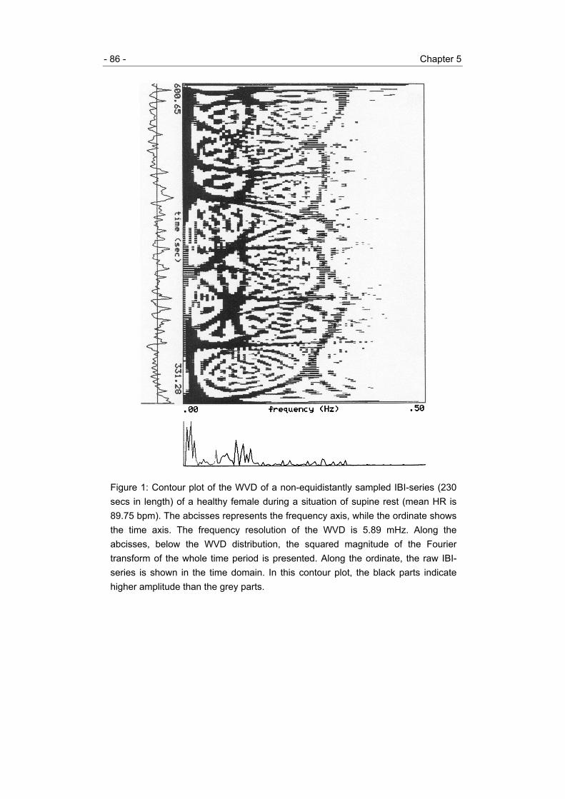
- 86 - Chapter 5
Figure 1: Contour plot of the WVD of a non-equidistantly sampled IBI-series (230secs in length) of a healthy female during a situation of supine rest (mean HR is89.75 bpm). The abcisses represents the frequency axis, while the ordinate showsthe time axis. The frequency resolution of the WVD is 5.89 mHz. Along theabcisses, below the WVD distribution, the squared magnitude of the Fouriertransform of the whole time period is presented. Along the ordinate, the raw IBI-series is shown in the time domain. In this contour plot, the black parts indicatehigher amplitude than the grey parts.

The Wigner-Ville distribution - 87 -
Figure 2: Contour plot of the WVD of a non-equidistantly sampled respiratory timeseries, of the same subject and time segment as shown in figure 1 (see forexplanation of abcisses and ordinate: figure 1.)

- 88 - Chapter 5
Figure 3: Contour plot of the WVD of a non-equidistantly sampled IBI-series of ahealthy male during a situation of rest (sitting position; time segment length 150sec). The frequency resolution is 3.34 mHz. (See for explanation of abcisses andordinate: figure 1.)

The Wigner-Ville distribution - 89 -
Figure 4: Contour plot of the WVD of a non-equidistantly sampled IBI-series of thesame subject as described in figure 3, during performance of the CWT (timesegment length 150 sec). The frequency resolution is 3.25 mHz. (See forexplanation of abcisses and ordinate: figure 1.)

- 90 - Chapter 5
Figure 5: Contour plot of the WVD of a non-equidistantly sampled systolic BP timeseries of a healthy female during a situation of supine rest. The frequencyresolution is 6.62 mHz. (See for explanation of abcisses and ordinate: figure 1.)

The Wigner-Ville distribution - 91 -
3.2 Example 1, rest situation
A typical WVD of an IBI-series of healthy young female during a situation of supinerest (figure 1) clearly shows the low, mid, and high frequency fluctuations as definedin the introduction. The low frequencies (<0.06 Hz) are fluctuating in amplitude overtime; the mid frequency fluctuations (around 0.1 Hz) are also not stationary presentthroughout the time series. These fluctuations appear to come in bursts: severalconcentrations are visible. The high frequency fluctuations (related to respiratorymodulation) also show non-stationarities over time. Figure 2 shows that these non-stationarities in the high frequency fluctuations as presented in figure 1 are indeedrelated to changes in respiration. Both figure 1 and 2 illustrate that the differentfrequency components within cardiovascular signals show complex changes, evenwithin a short time period of 230 sec and during a situation of supine rest.
3.3 Example 2, mental stress
During performance of a mental stress task, HR and HR variability can changedramatically. In our example, the heart rate of a young male increased from 53.25bpm (variation coefficient: 2.67%) during rest (figure 3), to 69.78 bpm (vc: 4.64%)during performance of the CWT (figure 4). Figure 3 and 4 visualize the changes thatoccur in time-frequency fluctuations during rest and during performance of the CWT.Both figures show the time course of the relevant frequency fluctuations. During theCWT, respiration rate increases and becomes very regular, causing a shift in theWVD of the respiratory related fluctuations in the IBI series to a higher frequency,which appears very stationary but only after about 30-40 sec. The other frequencycomponents also show that initial changes in cardiovascular fluctuations duringperformance of a mental stress task may differ from the changes that occur duringthe later part of the task. These examples indicate that the WVD may help to unravelthe relevance of initial time-frequency changes versus sustained changes in theunderstanding of cardiovascular control mechanisms during mental stress.
3.4 Example 3, cross terms
The non-stationary and discontinuous pattern (or bursts) of the mid frequencyfluctuations around 0.1 Hz is also observed in the WVD of systolic BP. This is clearlyvisible in figure 5. However, figure 5 also shows a ‘regular’ discontinuous pattern atabout 0.2 Hz. At the same frequency in the squared magnitude of the Fouriertransform of this signal, there is almost no activity present. Figure 5 is presented here

- 92 - Chapter 5
as an illustration of the phenomenon of cross terms in the WVD. Smoothing helps toreduce the disturbance of these ‘ghost’ curves (section 2.1).
4 Conclusion
The Wigner-Ville distribution offers a promising approach to study details of time-frequency relationships of cardiovascular time series within psychophysiologicalresearch. The fact that no assumptions need to be made on the stationarity of thedata, makes the method preferable to other spectral methods when analyzingspontaneous cardiovascular fluctuations over time. Two-dimensional presentation ofthe frequency related amplitude changes over time by means of WVD contour plotsoffers an elegant approach to study cardiovascular fluctuations during rest and tasksituations. Analysis of cardiovascular fluctuations by means of this method mayfurther extend our knowledge on the mechanisms of cardiovascular control duringsituations of rest and mental stress.
Appendix
A.1 Implementation of the discrete Wigner-Ville distribution
Let [ ]{ }, 1, 2,...,x n n N= be an equidistantly sampled time series of odd length,
12 1N N= + , and [ ]{ }1 1, ,...,v i i L L= − a window function of odd length, 12 1L L= + . T isthe total measuring time of the time series and t T N∆ = is the sample interval. T ′ isthe duration of the window function, i.e., T L t′ = ∆ . Calculate the analytical form [ ]z nof [ ]x n and define
[ ]nk i = [ ] [ ] [ ] [ ]v i z n i v i z n i∗ ∗⋅ + ⋅ − ⋅ −
for 1,2,...,n N= , 1 1,...,i L L= − . The DWVD (3) becomes:
[ ],W n k = [ ]1
1
42
ikL jL
ni L
k i eπ− ⋅
=−
⋅ ⋅∑ (A1)
for 1,2,...,n N= , 12 1N N= + , 0,1,..., 1k L= − . Define 2k k′ = and rewrite (A1):
[ ],W n k′ = [ ], 2W n k = [ ]1 2
10
2mkL jL
k nm
C k m L eπ− − ⋅
=
⋅ − ⋅∑ =
= [ ]{ }1 12 DFT , ,...,k nC k i i L L⋅ = − (A2)
in which12 kLjL
kC eπ ⋅
=

The Wigner-Ville distribution - 93 -
(Boashash & Black, 1987; Boashash, 1991). DFT in (A2) is a standard discreteFourier transform of the points [ ]{ }1 1, ,...,nk i i L L= − . The negative frequencycomponents are zero as a consequence of the fact that [ ]z n is analytical. So, thefrequency resolution is doubled: instead of 1 1L + positive frequency components at
kf k T ′= , 10,1,...,k L= , there are L positive frequency components at the frequencypoint 2kf k T′ ′ ′= , 0,1,..., 1k L′ = − . Compare this with the frequency resolution of thespectrum of [ ]x n , which is defined at the positive frequency points kf , 10,1,...,k N= .If the window length equals half the number of time points, i.e., 1 1L N= + , thefrequency resolution of the DWVD equals the frequency resolution of the spectrum.
In conclusion, the DWVD can be calculated using a standard discrete Fouriertransform. An efficient routine to calculate the DFT of an arbitrary number of data isthe chirp Z-transform (CZT) (Oppenheim & Schafer, 1975).
A.2 Heart rate variability spectra based on non-equidistant sampling
The methods of Rompelman (1985) and Mulder (1988), to estimate spectra of(cardiovascular) time series based on non-equidistant sampling of the R-waveoccurence times, are as follows.At the detection times it of the R-waves, samples ix , 1,2,...,i N= , are taken of acardiovascular signal. These samples are represented by a series of delta pulses:
( ) ( )1
N
i i ii
p t x t t tδ=
= ∆ −∑ (A3)
with 1i i it t t −∆ = − . This is called a cardiovascular time series. The Fourier transform ofthe function ( )p t is:
( )kX f = ( ) 2 kjf tp t e dtπ+∞ −
−∞⋅∫ = 2
1
k i
Njf t
i iix t e π−
=
∆ ⋅∑ (A4)
with kf k T= , 0,1,2,...k = , and T is the total measuring time (Mulder, 1988). Thespectrum P of the function ( )p t is calculated from (A4) by:
( ) ( ) ( )2k k kP f X f X f T∗=
(Bendat & Piersol, 1986).In case the time series is a heart rate time series, we take 1i ix t∆ = in (A4)
(Rompelman, 1985).

- 94 - Chapter 5
References
Akselrod, S., Gordon, D., Madwed, J.B., Snidman, N.C., Shannon, D.C., and Cohen,R.J. (1985). Hemodynamic regulation: investigation by spectral analysis. Am. J.Physiol., 249, H867-H875.
Allen, J.B. and Rabiner, L.R. (1977). A unified approach to short-time Fourieranalysis and synthesis. Proc. IEEE, 65, 1558-1564.
Bendat, J.S., and Piersol, A.G. (1986). Random data, analysis and measurementprocedures (2nd edition). John Wiley and Sons, Inc., New York.
Boashash, B. (1988). Note on the use of the Wigner distribution for time-frequencysignal analysis. IEEE Trans. ASSP-36, 1518-1521.
Boashash, B. (1991). Time-Frequency Signal Analysis. In: Haykin, S. (Ed.):Advances in Spectrum Analysis and Array Processing, Volume I (pp. 418-517).Prentice Hall, Englewood Cliffs, New Jersey.
Boashash, B., and Black, P.J. (1987). An efficient real-time implementation of theWigner-Ville distribution. IEEE Trans. ASSP-33, 1611-1618.
Claassen, T.A.C.M., and Mecklenbräuker, W.F.G. (1980). The Wigner distribution - Atool for time-frequency signal analysis. Part II: Discrete-time signals. PhilipsRes. J., 35, 276-300.
Cohen, L. (1989). Time-frequency distributions - a review. Proc. IEEE., 77, 941-981.Kitney, R.I. (1975). Entrainment of the human RR interval by thermal stimuli. J.
Physiol. Lond., 252, 37P-38P.Kootsookos, P.J., Lovell, B.C., and Boashash, B. (1992). A unified approach to the
STFT, TFDs and instantaneous frequency. IEEE Trans. Signal Processing, 40,1971-1982.
Malliani, A., Lombardi, F., Pagani, M., and Cerutti, S. (1990). The neural regulation ofcirculation explored in the frequency domain. J. Auton. Nerv. Syst., 30, S103-S108.
Mulder, G., and Mulder, L.J.M. (1981). Information processing and cardiovascularcontrol. Psychophysiology, 14, 392-402.
Mulder, L.J.M. (1988). Assessment of cardiovascular reactivity by means of spectralanalysis. Ph.D. Thesis, Groningen: University of Groningen.
Oppenheim, A.V., and Schafer, R.W. (1975). Digital signal processing. Prentice-Hall,Inc., Englewood Cliffs, New Jersey.
Parati, G., Castiglioni, P., Di Renzo, M., Omboni, S., Pedotti, A., and Mancia, G.(1990). Sequential spectral analysis of 24-hour blood pressure and pulseinterval in humans. Hypertension, 16, 414-421.

The Wigner-Ville distribution - 95 -
Rompelman, O. (1985). Spectral analysis of heart-rate variability. In: Orlebeke, J.F.,Mulder, G., and Van Doornen, L.J.P. (Eds.): Psychophysiology ofcardiovascular control (pp:315-331). Plenum Press, New York & London.
Saul, J.P., Berger, R.D., Albracht, P., Stein, S.P., Chen, M.H., and Cohen, R.J.(1991). Transfer function analysis of the circulation: unique insights intocardiovascular regulation. Am. J. Physiol., 261, H1231-H1245.
Ville, J. (1948). Théorie et applications de la notion de signal analytique. Cables etTransmission, 2eA, 1, 61-74.
Weber, E.J.M., Molenaar, P.C.M., and Van der Molen, M.W. (1992). A nonstationaritytest for the spectral analysis of physiological time series with an application torespiratory sinus arrhythmia. Psychophysiology, 29, 55-65.
Wesseling, K.H., and Settels, J.J. (1985). Baromodulation explains short-term bloodpressure variability. In: Orlebeke, J.F., Mulder, G., van Doornen, L.J.P. (Eds.):Psychophysiology of cardiovascular control (pp:69-97). Models, methods anddata. New York: Plenum Press.
Wigner, E. (1932). On the quantum correction for thermodynamic equilibrium. Phys.Rev., 40, 749-759.

- 96 - Chapter 5
CHAPTER 6THE EXPONENTIAL DISTRIBUTION APPLIED TO NON-EQUIDISTANTLY SAMPLED CARDIOVASCULAR TIMESERIES
Computers and Biomedical Research 29:174-193, 1996
H.G. van Steenis, J.H.M. Tulen
Department of Psychiatry, Erasmus University Rotterdam


The exponential distribution - 99 -
Beat-to-beat fluctuations in cardiovascular time series comprise different frequencycomponents which can be employed to describe autonomic regulatory processes.The exponential distribution (ED) is presented here as a specific time-frequencydistribution which has the potential to describe the time-related changes in thefrequency content of these cardiovascular fluctuations. The ED has as advantagethat it gives a good suppression of the cross terms, a characteristic feature of bilineartime-frequency distributions. An implementation to apply the ED to non-equidistantlysampled cardiovascular time series is provided. Applications of the ED to variousclinical and experimental human cardiovascular time series show that the ED can bean important aid to describe and interprete time-varying frequency components ofcardiovascular signals such as heart rate, interbeat interval, blood pressure andrespiration.
1 Introduction
The conventional method to study the dynamics of cardiovascular controlmechanisms is to estimate the variability spectra of the beat-to-beat fluctuations inheart rate (HR) and blood pressure (BP). These fluctuations in HR and BP areusually characterized by three spectral peaks in a frequency range of 0.01 to 0.50Hz:• a low frequency peak around 0.04 Hz,• a mid frequency peak around 0.1 Hz, and• a high frequency peak between 0.20-0.35 Hz.These peaks are believed to contain differential information related to eithersympathetic and/or parasympathetic processes within the cardiovascular controlsystem [1-4]: whereas respiratory-related high frequency fluctuations in HRparticularly reflect cardiac vagal (parasympathetic) tone, low and mid frequencyfluctuations in HR and especially BP may reflect sympathetic processes.
To estimate HR spectra and spectra of other cardiovascular signals, severalmethods have been developed. Most of these methods are based on equidistantsampling of the cardiovascular signals, in order to produce various time series ofcardiovascular quantities such as interbeat intervals or systolic BP (SBP). Spectracan then be calculated using a fast Fourier transform. However, HR is a frequencymodulated signal [5], whereas SBP and diastolic BP (DBP) are frequency andamplitude modulated signals [6]. We recently presented a method to computespectra of cardiovascular time series by means of non-equidistant sampling of the R-waves [7] based on the assumptions of Rompelman [5] and Mulder [6]. Non-
- 100 - Chapter 6
equidistant sampling of the HR signal or other cardiovascular signals guarantees thatwhenever time relationships between signals have to be studied (such as betweenHR and SBP), there are no relative time shifts between the time series or the relativetime shifts are constant over time. Computation of variability spectra and cross-spectra by means of non-equidistant sampling of the cardiovascular time series havethe advantage that these methods take into account both the frequency andamplitude modulation properties of these signals.
Spectral analysis is usually performed on consecutive time-segments rangingfrom 2–5 min, under the assumption that these time-segments can be consideredstationary. But even on this time-scale, the spontaneous cardiovascular fluctuationsare, in general, not completely stationary. This makes the spectra of the consecutivesegments less appropriate to examine changes in frequency components over time.For each segment, the time-varying frequency components will accumulate into widefrequency bands within the overall power spectrum. Furthermore, the high segment-to-segment variations in the power of the different frequency components over time[8] suggest that a more detailed analysis of time-frequency relationships iswarranted. These relationships can be described with a (joint) time-frequencydistribution (TFD). A TFD describes the frequency changes of the signal as a functionof time, while allowing non-stationarities. At each instant of time, a TFD shows thefrequencies that exist at that time. A well-known TFD is the Wigner-Ville Distribution(WVD; [9-14]). Novak & Novak [15] were the first to apply the WVD to cardiovasculartime series. In this paper, we will explore the possibilities of the exponentialdistribution (ED; [16]) to describe time-frequency relationships of variouscardiovascular time series. The ED is a modified WVD, which diminishes the effectsof the so-called cross terms. These cross terms are artefacts in a TFD due to thebilinearity of the TFD; cross terms are considered to be a drawback of the WVD.
Our aim of this paper is to apply the exponential distribution to non-equidistantly sampled cardiovascular time series. The implementation of the methodinto a computer program is provided. Furthermore, the applicability of the method tostudy details of cardiovascular time-frequency relationships is illustrated on bothclinical and experimental human data.

The exponential distribution - 101 -
2 Theory
2.1 Spectral analysis of non-equidistant cardiovascular time-series
The estimation of HR variability (HRV) spectra based on non-equidistant sampling ofthe R-wave incidences was first introduced by Rompelman [5]. The R-waves aredetected and represented by Dirac delta pulses ( )it tδ − at the incidence times it ,1,2,...,i N= . These delta pulses form the signal:
( ) ( )1
N
ii
p t t tδ=
= −∑ (1)
Such a series of consecutive R-wave incidences is called a HR signal or HR timeseries.
The Fourier transform of the function ( )p t is:
( ) ( ) 2 2
1
k k i
Njf t jf t
C ki
X f p t e dt eπ π+∞ − −
−∞=
= ⋅ =∑∫ (2)
in which kf k T= , 0,1,...,k = and T is the total record time. The spectrum CP of thefunction ( )p t is [17]:
( ) ( ) ( )2C k C k C kP f X f X f
T∗= ⋅ ⋅ (3)
and is estimated using the right part of equation (2). This spectrum is based on non-equidistant sampling, the delta pulses are occurring at the R-wave incidences. Thespectrum PC is called the spectrum of counts (SOC).
Let ( )p t be a HR time series of consecutive R-wave incidences at times it ,1,2,...,i N= . The time-intervals it∆ between the R-waves or interbeat intervals iI
(IBIs) are defined by iI = it∆ = 1i it t −− for 1,2,...,i N= (the first interval starts at R-waveincidence 0t ). The total record time T is
1
N
ii
T t=
= ∆∑ .
The mean sample interval t∆ or mean IBI I is T N . The ‘sample frequency’ isdefined by Sf = 1 I = N T (this is also called the ‘mean HR’) The ‘Nyquist frequency’is defined by 2N Sf f= . The frequency resolution is 1f T∆ = .
Prior to the calculation of the spectrum of a time series, it is customary tosubtract the DC of the time series. In case of an HR signal, DC-correction isperformed by subtracting a sequence of N delta functions from the original deltaseries ( )p t in equation (1). These delta functions are placed at equal intervals I , themean IBI. The function ( )p t then becomes [6]:
( ) ( ) ( )1 1
N N
ii i
p t t t t i Iδ δ= =
= − − − ⋅∑ ∑
- 102 - Chapter 6
At the R-wave incidences, samples of other cardiovascular signals can beobtained: the SBP or DBP can be determined, the IBI since the last R-waveincidence can be calculated, or a sample of the respiration (RSP) signal can betaken. In this way, a collection of data points on a beat-to-beat basis is obtained.Such a series is called a cardiovascular time series. Mulder [6] introduced a methodto calculate the spectrum of these non-equidistantly sampled signals (see also VanSteenis et al., [7]).
Let ix , 1,2,...,i N= be the samples of a cardiovascular signal taken at the R-wave incidences it , 1,2,...,i N= . The R-wave incidences are again represented bythe delta functions ( )it tδ − , but now they have weights i ix t∆ in which it∆ is the timeinterval 1i it t −− . Together they form the function ( )p t :
( ) ( )1
N
i i ii
p t x t t tδ=
= ∆ ⋅ −∑The Fourier transform of the function ( )p t is:
( ) ( ) 2 2
1
k k i
Njf t jf t
k i ii
X f p t e dt x t eπ π+∞ − −
−∞=
= ⋅ = ∆ ⋅∑∫ (4)
The spectrum P of the function ( )p t is:
( ) ( ) ( )2k k kP f X f X f
T∗= ⋅ ⋅ (5)
and is estimated using the right part of equation (4).DC-correction is applied by subtracting a weighted mean of the samples ix
from each sample. This weighted mean has the form:
1
1 N
W i ii
x x tT =
= ∆∑and (4) becomes:
( ) ( ) 2
1
k i
Njf t
k i W ii
X f x x t e π−
=
= − ∆ ⋅∑ (6)
2.2 The Wigner-Ville distribution
The traditional method to estimate the power spectrum of a stationary stochasticprocess ( )x t is the calculation of the Fourier transform of the autocorrelation function(ACF) of ( )x t :
( ) ( ) 2 jfx xS f R e dπ ττ τ
+∞ −
−∞= ∫ (7)
in which
( )xR τ = ( ) ( )E x t x t τ∗ ⋅ +

The exponential distribution - 103 -
is the ACF of the process ( )x t (* denotes the complex conjugate) [17]. For astationary process ( )x t , the ACF ( )xR τ is only dependent on the time lag τ and isnot dependent on time t . This property does not hold for non-stationary stochasticprocesses. In that case, the ACF of a stochastic process ( )x t becomes [17]:
( ),xR t τ = ( ) ( )2 2E x t x tτ τ∗ + ⋅ − .
Substituting this ACF in (7) yields a time-dependent spectral representation of ( )x t ,given by:
( ) ( ) 2, , jfx xS t f R t e dπ ττ τ
+∞ −
−∞= ∫
it follows that:
( ) ( )2, ,2 2
jfx xS t f E x t x t e d E W t fπ ττ τ τ
+∞ ∗ −
−∞
= + − ⋅ = ∫
in which [13,17]:
( ) 2,2 2
jfxW t f x t x t e dπ ττ τ τ
+∞ ∗ −
−∞
= + − ⋅ ∫ . (8)
The function ( ),xW t f is called the Wigner distribution (WD) of the stochastic process( )x t [9,11,13].
The discrete time equivalent of (8) for a random process ( )x t is [18]:
( ) ( ) ( ) 4, 2 j i t fx
iW n t f t x n t i t x n t i t e π
∞∗ − ⋅ ∆ ⋅
=−∞
∆ = ∆ ∆ + ∆ ∆ − ∆ ⋅∑( ..., 2, 1,0,1, 2,...n = − − ), in which t∆ is the sample interval. 1Sf t= ∆ is the samplefrequency. This function is periodic, with period 1f = 1 2 t∆ = 2Sf . This means thatfrequency components of the signal outside the frequency range [ ]1 12, 2f f− will befolded within this region, i.e., aliasing will occur. There are two methods to avoid this[12,19]:1) make sure that the frequency components outside [ ]1 12, 2f f− are zero; this canbe done by oversampling the signal by, at least, a factor four of the Nyquistfrequency, which is the highest frequency in the signal, i.e., 1 2 Nf f≥ and 4S Nf f≥ ;or2) make sure that the negative frequency components are zero; in this case thefrequency components in the region [ ]1 12,f f are zero and cannot disturb thefrequency components in the region [ ]10, 2f ; this can be done by using analyticalsignals.An analytical signal is a signal without negative frequency components. It is the dualof causal signals in the time domain [17]. Analytical signals can be sampled at a ratewhich is at least twice the Nyquist frequency, i.e., 2S Nf f≥ . In fact, the sample

- 104 - Chapter 6
frequency is doubled by producing an imaginary part to the real non-analytical signalin order to get the analytical form [19]. For an analytical stochastic process z(t), thefunction ( ),zW t f is called the Wigner-Ville distribution (WVD; [10,11,13]):
( ) 2,2 2
jfzW t f z t z t e dπ ττ τ τ
+∞ ∗ −
−∞
= + − ⋅ ∫ (9)
There is a second reason to use analytical signals [19]: real non-analyticalsignals can produce low-frequency artefacts in the Wigner distribution. These are aresult of interactions between positive and negative frequency components.Annihilation of the negative frequency components by using the analytical form of areal signal prevents these interactions. The interactions between positive andnegative frequencies are comparable to the appearance of ‘ghost’ curves betweentwo positive components.
2.3 Properties of TFDs
A TFD should reflect the energy distribution of the signal, both over time andfrequency. Therefore, a set of properties has been formulated which should apply toan ideal TFD [13,14,20]:P1: the TFD is real-valued;P2: integration over both time and frequency yields the total energy of the signal;P3: integration over time yields the spectral density of the signal;P4: integration over frequency yields the instantaneous power of the signal;P5: averaging over frequency yields the instantaneous frequency;P6: averaging over time yields the group delay;P7: the TFD satisfies the weak finite time support: if the signal is zero outside atime segment, then the TFD is zero outside this time segment;P8: the TFD satisfies the weak finite frequency support: if the signal is zerooutside a frequency segment, then the TFD is zero outside this frequency segment;P9: the TFD is positive.The short-time Fourier transform (STFT; [21]) only satisfies P1 and P9; the WVDsatisfies all except P9 [13,14].
2.4 Cross terms and the exponential distribution
A limitation of the WVD is the appearence of spectral cross terms, or ‘ghost’ curves inthe time-frequency domain. These cross terms are artefacts, which are due to thebilinear nature of the WVD (equation (9)) [13,14]. To understand this notion we workout the WVD of the sum of two pure sine waves [14]:

The exponential distribution - 105 -
( ) 1 22 21 2
jf t jf tz t A e A eπ π= +
The WVD of this analytical function consists of two autoterms and a cross term ( ( )δ iis the Dirac delta function):
( ) ( ) ( )2 21 1 2 2, cross termW t f A f f A f fδ δ= − + − + (10)
The cross term has the following form:( ) ( )( )1 2
1 2 2 1cross term 2 cos 22
f fA A f f f tδ π
+ = ⋅ − ⋅ −
(11)
The first two terms on the right hand side of (10) are the autoterms, they are theexpected components in the time-frequency plane at the frequencies 1f and 2f ofthe sine waves (compare this with the power spectrum of a sine wave). The resultingcross term, given in (11), is located halfway the two autoterms and the form of thecross term is sinusoidal. The cross terms in the WVD of a signal can also occur atthe position of the autoterms; they obscure the true time-frequency distribution andthey hamper the interpretation of the distribution.
An approach to diminish the cross terms is the use of the exponentialdistribution (ED), or Choi-Williams distribution, introduced by Choi & Williams [16]. Incomparison to the WVD, the ED has lower cross terms amplitudes, but it contains thesame information in the autoterms as the WVD [13]. This is achieved by convolutingthe function ( ) ( )2 2z t z tτ τ∗+ ⋅ − in (9), as a function of t , with an exponential kernelwhich has the form:
( ) 2 242,
4tK t e σ τ
σστπτ
−= ⋅ ,
in which σ is a parameter. For an analytical stochastic process ( )z t the ED has theform [16]:
( ) ( ) * 2, ,2 2
jfzE t f K u t z u z u du e dπ τ
στ ττ τ
+∞ +∞ −
−∞ −∞
= − ⋅ + − ⋅
∫ ∫
For large σ , the ED is almost equal to the WVD. Smaller values of σ will suppressthe cross terms. 2σ = has been found to be a good compromise for our applications.The ED satisfies the properties P1 through P6 (section 2.3). If σ is sufficiently large,the ED will also satisfy P7 and P8 [13,14,16].

- 106 - Chapter 6
2.5 The discrete exponential distribution
The discrete exponential distribution (DED) of a discrete analytical time series [ ]z n ,1,2,...,n N= is defined by [13,16]:
[ ] [ ]1 2 2
1 1
4 42, 2 ,
4
iMLm i j ik L
i L m ME n k e k n m i e
iσ πσ
π− − ⋅
=− =−
= ⋅ ⋅ + ⋅
∑ ∑ (12)
in which the kernelfunction [ ],k n i is defined by:
[ ] [ ] [ ] [ ] [ ],k n k v i z n i v i z n i∗ ∗= ⋅ + ⋅ − ⋅ − (13)
for 1,2,...,n N= , 0,1,..., 1k L= − and 12 1L L= + , L must be odd. L can be equal to N .[ ]v i is a window function of odd length L . [ ]v i is zero outside the segment [ ]1 1,L L− .
σ is a parameter. 12 1M M= + , M must be odd, and M can be equal to L . Thefactor 4 in the exponent and the factor 2 before the summation in equation (12) arethe result of the transformation of the continuous 2τ into the discrete variable i .
3 Methods
3.1 Implementation of the exponential distribution
The ED can only be applied to equidistantly sampled analytical signals. HR timeseries and cardiovascular time series are non-equidistant time series (both series willbe called cardiovascular time series from now on). In order to calculate the DED of acardiovascular time series, this series has to be transformed into an equidistantanalytical time series. Let ( )p t be a cardiovascular time series, according to section2.1. The first step is to calculate the complex Fourier transform, using equation (2) or(6), of this ( )p t . This results in an equidistant complex series in the frequencydomain. This series can be transformed back to the time domain with the well-knowninverse discrete Fourier transform (DFT). The number of R-waves in ( )p t andaccordingly the number of complex data in the frequency domain is generally not apower of two. Furthermore, it can be an odd number. Therefore, a fast Fouriertransform (FFT) cannot be used here. An efficient method to calculate the DFT or theinverse DFT of an arbitrary number of data is the chirp Z-transform (CZT) resp.inverse chirp Z-transform [22]. So, the second step is to apply the inverse CZT to thecomplex series in the frequency domain in order to get the desired equidistant timeseries in the time domain. It guarantees the same time resolution as the original timeseries. And the power spectrum of the equidistant series, calculated with the DFT,will be equal to the power spectrum of the non-equidistant series, calculated with

The exponential distribution - 107 -
equation (3) or (5). The next step is to calculate the analytical form of the resultingequidistant cardiovascular time series. One method, using the DFT, in this case theCZT, is described by Boashash & Reilly [23]. In short, this method calculates thecomplex Fourier transform of the time series, annihilates the negative frequencycomponents and multiplies the positive frequency components by two, andtransforms the result back to the time domain. An alternative way to produce theanalytical form is to use the Hilbert transform [17]. A FIR filter implementation of theHilbert transform is discussed by Boashash & Black [18]. The DED of the resultingequidistant analytical cardiovascular time series can be calculated as follows. Let[ ]z n , 1,2,...,n N= be a discrete equidistant analytical cardiovascular time series and[ ]v i , 1 1,...,i L L= − a window function of odd length 12 1L L= + . T is the total
measuring time and t T N∆ = is the sample interval. T ′ is the duration of the windowfunction, i.e., T L t′ = ∆ . Define:
[ ] [ ]2 2
1
42 ,
4
iMm i
nm M
k i e k n m ii
σσπ
−
=−
= ⋅ ⋅ +∑
(see equation (13)) and
[ ]12 LjL
LC eαπ
α =
Define 2k k′ = and rewrite (12):
[ ] [ ] [ ] [ ]1
21
0
, , 2 2L
j ik LL n
lE n k E n k C k k l L e π− ⋅
=
′ = = ⋅ − ⋅∑for 0,1,..., 1k L′ = − . Thus, the DED consists of the DFTs of the series [ ]nk i ,
1 1,...,i L L= − for each 1,2,...,n N= :
[ ] [ ] [ ]{ }n 1 1, 2 DFT k , ,...,LE n k C k i i L L′ = ⋅ = − (14)
The negative frequency components are zero as a consequence of the fact that [ ]z nis analytical; thus, the frequency resolution is doubled: instead of 1 1L + positivefrequency components at kf k T ′= , 10,1,...,k L= , there are L positive frequencycomponents at the frequency points 2kf k T′ ′ ′= , 0,1,..., 1k L′ = − , i.e., the frequencyresolution of the DED is 1 2f T′ ′∆ = . Note that the spectrum of the original time series[ ]x n is defined at the frequency points kf k T= , 0,1,..., 2k N= , i.e., the frequency
resolution is 1f T∆ = .Equation (14) can easily be implemented in a computer program. One can use theCZT to calculate the DFT of the odd number of data in (14). Our CZT-routine comesfrom MicroWay (387FFT, version 1.00, MicroWay Inc.). Equation (14) has to becalculated for each n . Together the results form the DED of the equidistant analytical
- 108 - Chapter 6
cardiovascular time series. The DED can visualized graphically as a function of timeand frequency by means of contour plots or three-dimensional surface plots.
3.2 Data acquisition
The applications presented in the next section were selected from severalexperiments in which cardiovascular parameters were studied during situations ofsupine rest, orthostatic stress, and controlled breathing, in healthy subjects, patientswith major depressive disorder [24], and patients with autonomic dysfunctions [25].ECG, BP, and RSP were recorded continuously during supine rest (10 min),controlled breathing by means of a metronome (3 min; 16 cls/min), orthostatic stress(8 min; passive 60° head-up tilt), controlled breathing (16 cls/min) during the 60°head-up tilt (3 min) and a 10 min-period of post-orthostatic supine rest. The ECG wasderived using a precordial lead, amplified by means of a polygraph (Nihon Kohden,Tokyo, Japan). BP was measured with a servoplethysmographic finger transducer(Finapres 2300 NIBP monitor, Ohmeda, Englewood, CO, USA). Thoracic RSP wasmeasured with an impedance plethysmograph (Nihon Kohden, Tokyo, Japan). Thesignals were digitized on an IBM compatible Personal Computer (Commodore PC60-III) equipped with an A/D converter (Advantech PC-LabCard model PCL-718).The sampling rate was 1024 Hz per channel. R-wave moments and R-R intervalswere detected with an accuracy of 1 ms; per R-R interval the SBP and DBP weredetected with an accuracy of 0.1 mmHg; and at each R-wave moment a sample ofthe RSP signal was taken as explained in section 2.1, these samples form the RSPtime series. The time series were divided in periods of 3 to 5 minutes correspondingto the above mentioned experimental procedures. Of each period, the powerspectrum and the DED, according to sections 2.1 and 3.1, were calculated.
4 Applications
4.1 Spontaneous cardiovascular fluctuations during supine rest
Figures 1, 2, and 3 present typical DEDs, computed from the corresponding HR,SBP, and RSP time series of a healthy subject during a 5 min period of supine rest(mean HR= 65.43 bpm, variation coefficient of the interbeat intervals: vc= 5.75%;mean SBP: 100.1 mmHg, vc= 4.57%). The overall spectra of HR and SBP (figures 1and 2) illustrate the three relevant frequency components around 0.04 Hz (low), 0.1Hz (mid), and around the dominant respiratory frequency at 0.30 Hz (high). The lowfrequencies (<0.06 Hz) of the DED of the HR and SBP time series show non-

The exponential distribution - 109 -
stationary fluctuations in both amplitude and frequency (figures 1 and 2). The midfrequency fluctuations around 0.1 Hz of the DED of both the HR and SBP time seriesare very irregular in appearance; some isolated areas of increased activity atcorresponding time points are apparent, reflecting the coherence between HR andBP fluctuations in the mid frequency range. The non-stationary fluctuations of theDED of the RSP signal (figure 3) are reflected at the corresponding frequencies ofthe DEDs of the HR and SBP time series (figures 1 and 2, respectively) due to therespiratory modulation of vagal-mediated cardiac control (HR) and/or due to themechanical effects of breathing (SBP). The DEDs of the HR, SBP and RSP timeseries nicely reflect the different frequency components within short-termcardiovascular fluctuations, but they also illustrate that even within a period of severalminutes and during a ‘stationary’ situation of supine rest, complex time-relatedchanges do occur.
4.2 Clinical example illustrating interference and correction of cross terms
The necessity to correct for cross terms in order to interprete time-frequencyrelationships accurately is illustrated by an example of a patient with pure autonomicfailure (PAF). Patients with PAF suffer from a complete or almost complete failure ofboth the sympathetic and the parasympathetic nervous system, resulting in dramaticreductions of both HR and BP variability [25]. Figure 4 presents the uncorrecteddiscrete WVD (DWVD), based on an IBI sequence of a patient with PAF during a 5min period of supine rest (mean HR=67.3 bpm, vc= 0.66%). Although the total powerof the overall spectrum of the IBI sequence is low (figure 4), two frequency bands stillare apparent: one peaks at about 0.03 Hz, the other peaks at the respiratoryfrequency at about 0.2 Hz. The fluctuations at about 0.4 Hz are harmonic frequenciesof the respiratory frequency. Frequencies at 0.1 Hz are completely absent, due to thestrongly diminished sympathetic tone in these patients. The DWVD does show thefrequencies at 0.03, 0.2 and 0.4 Hz, but halfway the low and respiratory peaks andhalfway the respiratory peak and the peak of the harmonic frequencies, two highlyirregular bands are visible: the ghost curves or cross terms (section 2.4). Notice thatthere is no activity at the corresponding frequencies in the overall spectrum.
Figure 5 presents the DED computed from the same IBI sequence: most ofthe cross terms are disappeared due to the procedures as described in section 2.4.The relevant frequency bands are now clearly represented in the time-frequencydistribution. Especially in subjects with autonomic failure, where evaluation ofminimal fluctuations in cardiovascular signals may have clinical relevance, adequatesuppression of cross terms is an essential feature of a time-frequency distribution.

- 110 - Chapter 6
Figure 1: DED of a non-equidistantly sampled HR time series (300 sec in length)of a healthy subject during supine rest. The abcisses is the frequency axis and theordinate is the time axis. Along the ordinate, the raw IBI-series is shown in the timedomain. Along the abcisses, the power spectral density (spectrum) of the wholetime series is presented. The scale of the spectrum, in this figure and the nextfigures, is always equal to the maximal component in the spectrum; in this casethe scale is 0.12 sec-2/Hz.

The exponential distribution - 111 -
Figure 2: DED of a non-equidistantly sampled SBP time series for the samesubject and time segment as presented in figure 1 (see figure 1 for explanation ofabcisses and ordinate). The scale of the spectrum is 2167.89 mmHg2/Hz.
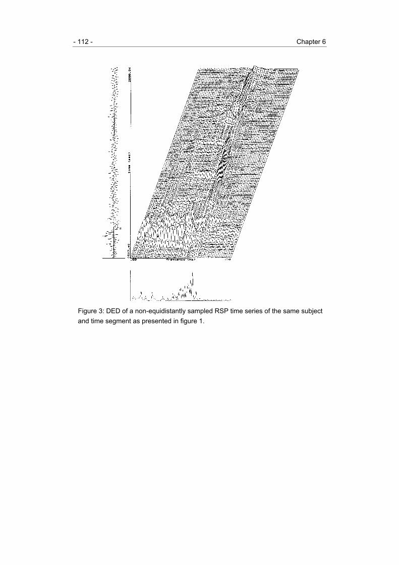
- 112 - Chapter 6
Figure 3: DED of a non-equidistantly sampled RSP time series of the same subjectand time segment as presented in figure 1.

The exponential distribution - 113 -
4.3 Specific examples of non-stationary time-frequency relationships
1a) Respiratory modulation of HR variabilityIn certain situations, interpretation of overall spectra of HR (and BP) variability maylead to erroneous conclusions if there is no information available of the respiratorysignal. Figures 6 and 7 illustrate the DEDs from corresponding HR and RSP timeseries of a depressed patient during a 4 min period of supine rest. The overallspectrum of the HR time series (figure 6; mean HR=68.38 bpm, vc=13.1%) showstwo clear broad-band frequencies: one around 0.1 Hz, a possible reflection ofsympathetic-mediated processes, and one around 0.25 Hz, reflecting respiratory-linked variations due to vagal-mediated cardiac control. The corresponding DEDillustrates a sudden shift from slow to faster frequencies, suggesting a dramaticchange in sympathetic modulation. However, as can be observed in figure 7, thecorresponding respiratory signal shows a change from a slow breathing frequency(about 0.1 Hz) to a faster breathing frequency (0.18-0.22 Hz). This time-relatedchange is evident in the DED, whereas the overall spectrum shows the two broad-band peaks corresponding to the change in breathing frequency. Therefore, in thisexample, both peaks in the HR spectrum primarily reflect respiratory-linked vagalactivity.
1b) Cardiac arrhythmiasThe DED of an IBI sequence of a depressed patient treated with the tricyclicantidepressant imipramine is presented in figure 8 (mean HR=79.74 bpm, vc=2.7%).The IBI sequence was derived from a 4 min period of supine rest and reflects a briefepisode of supraventricular cardiac arrhythmias. This brief period of arrhythmiasaffects all frequency components in the DED due to the rapid fluctuations in thesuccessive IBI lengths. Furthermore, there appears a high peak around the Nyquistfrequency in the DED. This peak is also visible in the overall spectrum of the IBIsequence, and interferes greatly with the respiratory-related high frequencies. Justbefore and during the arrhythmic period, there is a slow trend in the IBI sequence. Inthe DED, this trend appears as a high peak in the low frequency range. In thespectrum, the low frequency peak is primarily caused by this temporary change.Notice the effect of the isolated arrhythmic artefacts later on in the IBI sequence. Thedelta-like peaks affect all frequency components in the DED. At the crosspoints withthe respiratory-related frequencies, the two components are superponated. Cardiacarrhythmias have a major impact on homeostatic cardiovascular processes asreflected in HR and BP variability; this example illustrates the extent to which isolatedgrouped arrhythmias disturb time-frequency distributions.

- 114 - Chapter 6
Figure 4: DWVD of a non-equidistantly sampled IBI time series of a patient withPAF during 5 min of supine rest. The scale of the spectrum is 0.0011 sec2/Hz. Thefigure is very irregular due to the cross terms. Note the two striking cross termbands.

The exponential distribution - 115 -
Figure 5: DED of the same IBI time series as in figure 4. The cross terms arealmost disappeared due to the smoothing effect of the ED.

- 116 - Chapter 6
Figure 6: DED of a non-equidistantly sampled HR time series of a depressedpatient during 4 min of supine rest. The scale of the spectrum is 0.49 sec-2/Hz.

The exponential distribution - 117 -
Figure 7: DED of the RSP time series of the same subject and time segment aspresented in figure 6. Note the sudden shift from slow to faster frequencies.

- 118 - Chapter 6
Figure 8: DED of an IBI time series of a depressed patient during 4 min of supinerest. The scale of the spectrum is 0.0095 sec2/Hz.

The exponential distribution - 119 -
Figure 9: DED of a SBP time series of a depressed patient dureing 4 min of headup tilt. The scale of the spectrum is 767.11 mmHg2/Hz. The initial cardiovascularreaction to the head up tilt is most prominent in the frequency components around0.1 Hz.
- 120 - Chapter 6
1c) Adjustments to sudden situational changesIn figure 9, the SBP sequence of a depressed subject reflects the initialcardiovascular reaction to the 60° head-up tilt procedure (mean SBP= 127.2 mmHg,vc= 4.20%). In the DED, the respiratory-related high frequencies are apparentthroughout the entire procedure. However, the transition from supine posture topassive standing causes a momentary increase in activity around 0.1 Hz, as anindication of an increase in sympathetic tone, which is evident also in the DED.However, its reflection in the overall spectrum erroneously suggests a sustainedpresence of these periodicities during the entire period. The DED illustrates that thepatient gets accustomed to the standing position: the activity around 0.1 Hzdiminishes rapidly and after that the DED shows some isolated moments of activity atthese frequencies. This example shows that initial cardiovascular adjustments tosudden situational changes can be visualized in detail by means of a DED.
5 Discussion
In this paper, an implementation to apply the exponential distribution to non-equidistantly sampled cardiovascular time series has been given. We used themethods of Rompelman [5] and Mulder [6] to transform the non-equidistantlysampled cardiovascular time series into equidistant time series. This enabled us tocalculate the DED of HR as well as IBI time series. Furthermore, using the CZTenabled us to calculate the Fourier transform of time series with lengths notnecessarily equal to a power of two.
The ED is a modified WVD. Implementations of the DWVD and/or DED havebeen discussed previously by Martin & Flandrin [26], Chester [27], Boashash & Black[18], Sun et al. [28], Boashash & Reilly [23]. A method to suppress cross terms in aDWVD has been discussed by Martin & Flandrin [26]. They used a symmetricnormalized time window and a time smoothing function. The effect of the timewindow is smoothing of the WVD in the frequency direction; thus, it will also spreadout the autoterms. The effect of the smoothing function is a reduction of the crossterms, but it has also a smoothing effect on the autoterms in the time direction.Therefore, the implementation of the DWVD by Martin & Flandrin does not satisfy theproperties P3-P8 (section 2.3). Novak & Novak [15] applied the DWVD, using FFTtechniques, to IBI, SBP, DBP, and RSP time series, each time series linearlyinterpolated to an equidistant time series. They implemented the method of Martin &Flandrin to correct for cross terms, using a computation algorithm of Peyrin & Prost[29]. We employed the ED because it has certain advantages over the forementioned

The exponential distribution - 121 -
method: the ED satisfies the advocated properties P1-P6 (section 2.3) for TFDs, forall values of σ . When the smoothing effect is too large, i.e. small σ ( 1σ ≤ ; [16]), theautoterms and the components in the time direction will be spread noticeably. Thus,P7 and P8 will not be satisfied. If σ is sufficiently large ( 1σ > ) then the ED willapproximately satisfy properties P7 and P8 [14]. Furthermore, for increasing σ , theED will become approximately equal to the WVD. According to Choi & Williams, agood choice of σ will be found between 0.1 and 10. Our DED examples ofcardiovascular time series, with 2σ = , show that the cross term suppression by theED is satisfactory without disturbing the autoterms too much.
Our applications illustrated the potential of the ED to study time-frequencyrelationships of and between cardiovascular time series. Complex time-varyingaspects of the relevant cardiovascular frequency components of HR, IBI, BP, andRSP time series could be made visible by means of the ED. Therefore, the ED canbe an important aid to describe and interprete the complex dynamics of autonomicregulatory processes.
References
[1] Sayers BMcA. Analysis of heart rate variability. Ergonomics 16: 17-32, 1973.[2] Akselrod S, Gordon D, Madwed JB, Snidman NC, Shannon DC, and Cohen RJ.
Hemodynamic regulation: investigation by spectral analysis. Am J Physiol 249:M867-M875, 1985.
[3] Tulen JHM, Smeets FML, Man in 't Veld AJ, Van Steenis HG, Van de WeteringBJM, and Moleman P. Cardiovascular variability after clonidine challenge:assessment of dose-dependent temporal effects by means of spectral analysis.Journal of Cardiovascular Pharmacology, 22: 112-119, 1993.
[4] Tulen JHM, Man in 't Veld AJ, AM van Roon, Moleman P, Van Steenis HG,Blankestijn PJ, and Boomsma F. Spectral analysis of hemodynamics duringinfusions of epinephrine or norepinephrine in men. Journal of AppliedPhysiology, 76(5): 1914-1921, 1994.
[5] Rompelman O. Spectral analysis of heart-rate variability. In: Psychophysiologyof Cardiovascular Control. Orlebeke JF, Mulder G, Van Doornen LJP (eds).New York & London: Plenum Press, pp:315-331, 1985.
[6] Mulder LJM. Assessment of cardiovascular reactivity by means of spectralanalysis (Ph.D. Thesis). Groningen: University of Groningen, 1988.
[7] Van Steenis HG, Tulen JHM, and Mulder LJM. Heart rate variability spectrabased on non-equidistant sampling: the spectrum of counts and the

- 122 - Chapter 6
instantaneous heart rate spectrum. Medical Engineering and Physics 16:355-362, 1994.
[8] Parati G, Castiglioni P, di Renzo M, Omboni S, Pedotti A, and Mancia G:Sequential spectral analysis of 24-hour blood pressure and pulse interval inhumans. Hypertension 16: 414-421, 1990.
[9] Wigner E. On the quantum correction for thermodynamic equilibrium. Phys Rev40: 749-759, 1932.
[10] Ville J. Théorie et application de la notion de signal analytique. Cables etTransmissions 2A(1): 61-74, 1948.
[11] Claassen TACM and Mecklenbräuker WFG. The Wigner distribution - a tool fortime-frequency signal analysis, part I: continuous-time signals. Philips Res J 35:217-250, 1980.
[12] Claassen TACM and Mecklenbräuker WFG. The Wigner distribution - a tool fortime-frequency signal analysis, part II: discrete-time signals. Philips Res J 35:276-300, 1980.
[13] Boashash B. Time-frequency signal analysis. In: Advances in SpectrumAnalysis and Array Processing, Vol. 1. S. Haykin, Ed. Englewood Cliffs, NJ:Prentice Hall, pp:418-517, 1991.
[14] Cohen L. Time-Frequency Analysis. Englewood Cliffs, NJ: Prentice Hall Inc,1995.
[15] Novak P and Novak V. Time/frequency mapping of the heart rate, bloodpressure and respiratory signals. Medical & Biological Engineering & Computing31(2): 103-110, 1993.
[16] Choi HI and Williams WJ. Improved time-frequency representation ofmulticomponent signals using exponential kernels. IEEE Trans Acoust SpeechSignal Proc ASSP-37: 862-871, 1989.
[17] Bendat JS and Piersol AG. Random Data, Analysis and MeasurementsProcedures, 2nd edition. New York: John Wiley and Sons, Inc., 1986.
[18] Boashash B and Black PJ. An efficient real-time implementation of the Wigner-Ville distribution. IEEE Trans Acoust Speech Signal Proc ASSP-33: 1611-1618,1987.
[19] Boashash B. Note on the use of the Wigner distribution for time-frequencysignal analysis. IEEE Trans Acoust Speech Signal Proc ASSP-36: 1518-1521,1988.
[20] Kootsookos PJ, Lovell BC, and Boashash B. A unified approach to the STFT,TFDs and instantaneous frequency. IEEE Trans. Signal Processing 40: 1971-1982, 1992.

The exponential distribution - 123 -
[21] Allen JB and Rabiner LR. A unified approach to short-time Fourier analysis andsynthesis. Proc IEEE 65: 1558-1564, 1977.
[22] Oppemheim AV and Schafer RW. Digital signal processing. Englewood Cliffs,NJ: Prentice-Hall Inc, 1975.
[23] Boashash B and Reilly A. Algorithms for time-frequency signal analysis. In:Time Frequency Signal Analysis – Methods and Applications, chapter 7. B.Boashash, Ed. Longman Cheshire, pp:163-181, 1992.
[24] Tulen JHM, Bruijn JA, De Man KJ, Pepplinkhuizen L, Van den Meiracker AH,and Man in 't Veld AJ. Cardiovascular variability in major depressive disorderand effects of imipramine or mirtazapine (org 3770). Journal of ClinicalPsychopharmacology 16: 135-145, 1996.
[25] Van den Meiracker AH, Tulen JHM, Man in 't Veld AJ, Balk AHMM, Van SteenisHG, and Schalekamp MADH. Blood pressure and heart rate variability in clinicalmodels of cardiac denervation, sympathicolysis and sympathico- andparasympathicolysis. J Hypertension, 11(suppl 5): S152-S153, 1993.
[26] Martin W and Flandrin P. Wigner-ville spectral analysis of nonstationaryprocesses. IEEE Trans Acoust Speech Signal Proc ASSP-33(6): 1461-1470,1985.
[27] Chester D. Discrete Wigner implementations. 1986 Int Symp Circuit and SystProc San Jose, 38-41, 1986.
[28] Sun M, Li CC, Sekhar LN, and Sclabassi RJ. Efficient computation of thediscrete pseudo-Wigner distribution. IEEE Trans Acoust Speech Signal ProcASSP-37: 1735-1742, 1989.
[29] Peyrin F and Prost RA. A unified definition for the discrete-time, discrete-frequency and discrete-time/frequency Wigner distribution. IEEE Trans AcoustSpeech Signal Proc ASSP-34: 858-867, 1986.

- 124 - Chapter 6

CHAPTER 7QUANTIFICATION OF THE DYNAMIC BEHAVIOR OVERTIME OF NARROW-BAND COMPONENTS PRESENT INHEART RATE VARIABILITY BY MEANS OF THEINSTANTANEOUS AMPLITUDE AND FREQUENCY
Submitted
H.G. van Steenis1, W.L.J. Martens2, J.H.M. Tulen1
1Department of Psychiatry, Erasmus Medical Center Rotterdam2PhyVision b.v., Gemert


Instantaneous amplitude and frequency - 127 -
Variability in heart rate sometimes shows oscillatory, sine-wave-like, or ‘deterministic’properties whereas under different circumstances the signals look ‘noisy’ or‘irregular’. Three oscillatory narrow-band components have been postulated to occurin spontaneous variability of heart rate within a time-scale of several minutes: low(0.02-0.07 Hz), mid (0.07-0.15 Hz), and high (0.15-0.50 Hz). Reduction of theseoscillations in disease states has been shown to be a powerful predictor of futureclinical events and mortality.
By applying Fourier transforms to quantify these three components, anobservation interval (or time window) of 2-5 minutes is usually chosen as acompromise to achieve an appropriate frequency-resolution. However, in thisobservation interval, the signal may be ‘non-stationary’, meaning that the statisticalproperties of the signals may change over time.
Given the fact of the three narrow-band components, this paper describes amethod to derive the shortest possible observation interval for each of thesecomponents, which is inversely related to the bandwidth of these three componentsas given by the uncertainty principle of Gabor. For the high-frequency component, if abandwidth of 0.35 Hz is postulated, such minimal observation interval tσ translatesinto a time-resolution t∆ of about 2.25 sec in the discrete time-domain. For the mid-frequency component, with a bandwidth of 0.08 Hz, this yields about 7.75 sec,respectively. If signal properties, such as amplitude (or envelope) and frequency, arecomputed at such proper and optimal time-resolution, adjacent points in time areindependent in a statistical sense, that means that these properties then areinstantaneous. In that case the amplitude and the frequency are called instantaneousamplitude and frequency. Computations over a shorter time interval yield adjacentlydependent points in time; if computed over a longer time interval, properties will beaveraged, i.e., smeared over time (as with Fourier analysis). This means that thepresented method does not introduce redundancy (by interpolation) nor smearingover time, so the instantaneous properties then can be related to the underlyingphysiological model that reacts on (non) stationary internal and externalcircumstances.
Recalling that cardiovascular signals may show waxing and waning ofoscillatory ‘deterministic’ and noisy ‘irregular’ properties in time, especially theoscillatory periods in time may be related to autonomic cardiac control processes. Inthis paper, in addition to the computation of the instantaneous amplitude andfrequency, a method is introduced to compute an index of the instantaneousbandwidth for the narrow-band components as a means to separate the oscillatoryand irregular periods in time.
- 128 - Chapter 7
1 Introduction
Heart rate variability is controlled by the autonomic nervous system and affected byexternal and internal factors, such as physical activities and locomotion, circadianrhythm and psychological influences. Furthermore, heart rate variability is altered in avariety of disease states; reduced variability has repeatedly been shown to be apowerful predictor of clinical events and mortality [e.g., 1,2].
The oscillatory sine-wave-like narrow-band fluctuations that occur in short-term heart rate variations originate from various sources in the autonomiccardiovascular control system. We mention three [3-12].1) Fluctuations in peripheral vasomotor tone related to thermoregulation, renin-angiotensin system activity, or other processes. The period length of thesefluctuations varies between 14-50 sec.2) Oscillations due to the baroreflex control of peripheral resistance, with a periodlength of about 10 sec; these oscillations may reflect sympathetic processes. And3) respiratory-related fluctuations, possibly reflecting cardiac parasympathetic(vagal) nervous activity; the period length of these fluctuations is about 3 sec.These oscillatory fluctuations are called short-term fluctuations. Spectral analysisaims at characterizing such oscillations in the frequency domain; three spectralranges or peaks can be discerned in:1) the low-frequency range: 0.02-0.07 Hz;2) the mid-frequency range: 0.07-0.15 Hz; and3) the high-frequency range: 0.15-0.50 Hz.The conventional observation interval or time window over which spectral analysis ofshort-term fluctuations is performed varies between 2-5 min, i.e., intervals longenough to measure the slow fluctuations of the low-frequency range. But even in atime interval as short as 2-5 min, the frequency content of heart rate variesconsiderably [13]. Apparently, the spontaneous fluctuations are too rapid to becaptured in observation intervals, even as short as a few minutes.
In general, heart rate variability is a dynamic ‘non-stationary’ signal [14]. Weuse the term ‘non-stationary signal’ in the sense of statistical properties of the signalchanging over time. This means that the characteristic spectral peaks, low, mid, andhigh, vary in time in their position on the frequency axis (frequency), energy (oramplitude), as well as in the spread or width of their peak (bandwidth). One canimagine an ‘instantaneous spectrum’ [15,16] at each instant in time. These‘instantaneous spectra’ visualize the time-varying characteristics of a signal. One wayto obtain these is by means of a time-frequency distribution, such as the Wigner-Ville

Instantaneous amplitude and frequency - 129 -
distribution [15,17] or the Exponential Distribution [18,19]. In this paper, we provide amethod to compute the time-varying ‘instantaneous spectrum’ quantitatively bymeans of the instantaneous amplitude (IA), frequency (IF), and the instantaneousbandwidth (IB). The method only applies to monocomponent signals of which theenergy is concentrated in one spectral peak. To approximate a monocomponentsignal, as close as possible, we decompose the heart rate variability signal with athree zero-phase band-pass filters into the three spectral peaks of interest: low, mid,or high. The time-varying properties of each of the three components can now bedescribed by means of the IA and the IF. The squared IA is a measure of theinstantaneous power or energy per unit time. The IF defines the frequency location ofthe spectral peak. The spread of the spectral peak is measured by means of the IB,being the associated standard deviation of the average IF. In our case, the so-calledinstantaneous bandwidth coefficient (IBC) is computed as an index for the IB. TheIBC may serve as a time-varying segmentator of oscillatory versus irregular periods:low values indicate oscillatory properties, high values indicate irregularities.
Our method was developed to gain information on the functioning of thesympathetic and parasympathetic processes within the cardiovascular control systemon the highest possible time-resolution as given by the uncertainty principle of Gabor.This time-resolution is different for the low-, mid-, and high-frequency components,that is, it is inversely related to the bandwidth of these three components. It meansthat the method does not introduce redundancy (by interpolation) or smearing overtime. Hence the parameters IA and IF of the fluctuations in low-, mid-, and high-frequency bands can now be totally related to external and internal time-varyingprocesses. For instance, under ambulatory conditions, the fluctuations can be relatedto body posture (lying, sitting, standing) and physical activities (walking), wherebyalso the time-varying spectral details of transitions between postures and activitiescan be examined. In the case of measurements in a controlled laboratoryenvironment, the fluctuations can be related to the effects of psychological, physical,or pharmacological challenge tests. In addition, a detailed description of IA and IF, inrelation to the IBC, in disease states associated with altered heart rate variability willcontribute to an increased understanding of the processes involved in the triggeringof clinical events or mortality.
In this paper we limit ourselves to the application of the method to the mid-and high-frequency band of heart rate variability time series. However, the methodwas developed to be applied to the three narrow-band (low-, mid-, and high-frequency) components of cardiovascular time series and also to respiratory signals.

- 130 - Chapter 7
2 Theory of instantaneous properties of narrow-band signals
In a first approximation, the instantaneous amplitude or envelope and instantaneousfrequency of a narrow-band oscillatory signal can be computed by rectificationfollowed by smoothing and by zero-crossing techniques respectively. The undistortedenvelope, that is the removal of the carrier oscillation frequency, can only beaccomplished via complex demodulation which is based on the so-called complexanalytical signal. This is explained in the next section.
2.1 Analytical signals and the instantaneous frequency
The (complex) analytical signal ( )ts [20] associated with a real signal ( )ts allows usto define the instantaneous amplitude, phase, and frequency of the real signal ( )ts .The real part of the analytical signal ( )ts equals the original real signal ( )ts . Theimaginary part is obtained from the real signal by means of the Hilbert transform[16,20,21]. The envelope or IA ( )ta and the instantaneous phase (IP) ( )tϕ aredefined as the modulus and the argument of the complex number ( )ts , respectively.The analytical signal can now be written in polar form ( ) ( ) ( )ˆ j ts t a t e ϕ= and visualizedas a moving vector in the complex plane. Furthermore, the IF can be defined as therate of change of the phase angle ( )tϕ [15,16,21]:
( ) ( )tdtdtfiϕ
π21
= . (1)
If the spectrum of ( )ta is contained in a frequency region 11 ωωω <<− and thespectrum of ( )tϕcos is zero for 1ωω ≤ , i.e., reflecting a slowly varying amplitudemodulation and a fast phase modulation, it can be proven that the analytical signal( )ts is a reliable and natural representation of the real signal ( )ts [16,21]. This means
that ( )ta , ( )tϕ , and ( )if t represent the IA, IP, and IF, respectively, of the real signal( )ts . Furthermore, Rihaczek [22] proved that under the same conditions, the time-
varying signal’s energy is in frequency concentrated in a single narrow frequencyrange at the IF ( )tff i= . See appendix A.1 for a further explanation of the analyticalsignal and the Hilbert transform.
Suppose that locally (in time) the analytical signal ( )ts is ‘multicomponent’[16,18,21]. This means that the signal’s energy is locally distributed in two or morefrequency peaks. In that case the IF has no physical meaning. Cohen [21 p.40]mentioned a few inconsistencies that may occur. For instance, the computed IF maynot be in the signal’s spectral region, even if the signal is band-limited. It maybecome negative, though the signal is analytical. Therefore, the IF has only meaningfor ‘monocomponent’ signals, for which there is only one time-varying spectral

Instantaneous amplitude and frequency - 131 -
concentration. The IF has no meaning for multicomponent signals with more than onespectral concentration. See appendix A.3 for a further description of the conceptsmulticomponent and monocomponent.
Concluding, our model signal is a band-limited, monocomponent, andanalytical signal. Of this signal the IF can be computed reliably and is meaningful.Furthermore, the spectral peak is concentrated at the IF on the frequency axis.
2.2 The Wigner-Ville distribution and the instantaneous frequency
A means to study the time-varying energy content and the time-varying IF is theWigner-Ville distribution. Ville introduced the Wigner-Ville distribution of an analyticalsignal ( ) ( ) ( )tjetats ϕ=ˆ [15,17,21,23,24,25]:
( ) ∫∞+
∞−
−⋅
−⋅
+= τττ τπ detstsftW jf2*
2ˆ
2ˆ, .
The Wigner-Ville distribution is a joint time-frequency distribution of an analyticalsignal ( )ts , which gives insight in the signal’s frequency distribution at every instant t .The Wigner-Ville distribution can help to analyze the structure of the components of( )ts . If the signal is multicomponent, the multiple components will cause cross terms
in the Wigner-Ville distribution [21,23]. In our case the signal is monocomponent andband-limited, so there is only one component in the time-frequency plane.
At each instant t , the frequency distribution ( )ftW , constitutes an‘instantaneous spectrum’ [15,16]. The area of ( )ftW , at time t is the instantaneouspower or energy per unit time and equals the squared IA [21,23]:
( ) ( )∫∞+
∞−= dfftWta ,2 .
The IF of an analytical signal ( )ts is defined as the derivative of the IP ( )tϕ (equation(1)). For a sinusoidal signal, this definition is unambiguous. The sinusoid is a sharpdelta peak in the time-frequency plane at the IF and has no spread, i.e., there is onlyone frequency present, namely at the IF. If the signal has (locally) a stochasticcomponent, this definition becomes harder to interpret because the frequencycontent is not concentrated in one delta peak. However, Ville showed that theconditional average
tf of the existing frequency components at a certain time t
equals the derivative of the phase at that time, i.e., the IF at time t is the firstconditional moment of the Wigner-Ville distribution with respect to frequency at time t[15,21,23]:
( )
( )( ) ( )tft
dfftW
dfftWff it
=′=⋅
=∫∫
∞+
∞−
∞+
∞− ϕπ21
,
,(2)
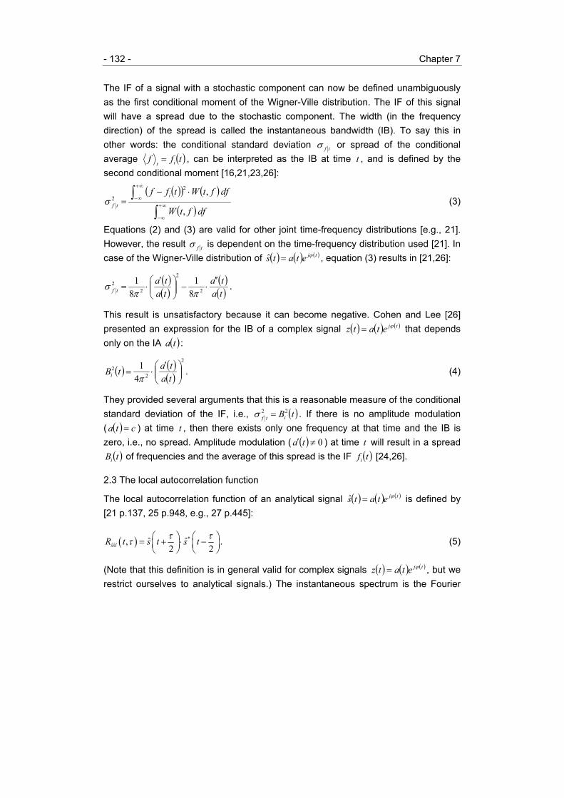
- 132 - Chapter 7
The IF of a signal with a stochastic component can now be defined unambiguouslyas the first conditional moment of the Wigner-Ville distribution. The IF of this signalwill have a spread due to the stochastic component. The width (in the frequencydirection) of the spread is called the instantaneous bandwidth (IB). To say this inother words: the conditional standard deviation f tσ or spread of the conditionalaverage ( )tff it
= , can be interpreted as the IB at time t , and is defined by thesecond conditional moment [16,21,23,26]:
( )( ) ( )
( )∫∫
∞+
∞−
∞+
∞−⋅−
=dfftW
dfftWtff i
tf,
,2
2σ (3)
Equations (2) and (3) are valid for other joint time-frequency distributions [e.g., 21].However, the result f tσ is dependent on the time-frequency distribution used [21]. Incase of the Wigner-Ville distribution of ( ) ( ) ( )tjetats ϕ=ˆ , equation (3) results in [21,26]:
( )( )
( )( )tata
tata
tf
′′⋅−
′⋅= 2
2
22
81
81
ππσ .
This result is unsatisfactory because it can become negative. Cohen and Lee [26]presented an expression for the IB of a complex signal ( ) ( ) ( )tjetatz ϕ= that dependsonly on the IA ( )ta :
( ) ( )( )
2
22
41
′⋅=
tatatBi π
. (4)
They provided several arguments that this is a reasonable measure of the conditionalstandard deviation of the IF, i.e., ( )tBitf
22 =σ . If there is no amplitude modulation( ( ) cta = ) at time t , then there exists only one frequency at that time and the IB iszero, i.e., no spread. Amplitude modulation ( ( ) 0≠′ ta ) at time t will result in a spread( )tBi of frequencies and the average of this spread is the IF ( )tfi [24,26].
2.3 The local autocorrelation function
The local autocorrelation function of an analytical signal ( ) ( ) ( )tjetats ϕ=ˆ is defined by[21 p.137, 25 p.948, e.g., 27 p.445]:
( ) *ˆˆ ˆ ˆ,
2 2sslR t s t s tτ ττ = + ⋅ −
. (5)
(Note that this definition is in general valid for complex signals ( ) ( ) ( )tjetatz ϕ= , but werestrict ourselves to analytical signals.) The instantaneous spectrum is the Fourier

Instantaneous amplitude and frequency - 133 -
transform of the local autocorrelation function; they are linked with each other bymeans of the Wiener-Khinchine theorem [27].
Both the IF ( )tfi and the IB ( )tBi of ( )ts can be written in terms of the localautocorrelation function. In case of the IF, an approximation for ( )tfi is obtained bysubstituting ( ) ( ) ( )tjetats ϕ=ˆ in ( )ˆˆ ,sslR t τ for hτ = :
( )ˆˆ ,sslR t h = 2 2
2 2
h hj t th ha t a t eϕ ϕ + − − + − ⋅
The argument of ( )ˆˆ ,ssiR t h is:
( )ˆˆarg ,sslR t h =2 2h ht tϕ ϕ + − −
≈ ( )h tϕ′⋅ .
Using equation (1) it follows that [28-31]:
( ) ( )ˆˆ1 arg ,12i sslf t R tπ
≈ (6)
Phase-shifts of 2π± due to the ambiguity of the inverse tangent do not occur in (6)because the phase-shifts are canceled in the difference of the phases in themultiplication of the right-hand complex conjugated product factors in (5).
In case of the IB, expanding ( )ˆˆ ,sslR t h gives us also an approximation for ( )tBi ,using the fact that ( ) 0≥ta :
( )( )
ˆˆ
ˆˆ
,1
,0ssl
ssl
R t hR t
− =( )22 21
h ha t a t
a t
+ − − ≈
( ) ( ) ( ) ( ) ( )
( )
2
22 2h ha t a t a t a t a t
a t
′ ′− + ⋅ − ⋅ =
( )( )
22
24a tha t
′⋅ (for small h ).
Comparing this result with equation (4), it follows that:
( ) ( )( )
ˆˆ22
ˆˆ
,11 1,0
ssli
ssl
R tB t
R tπ
≈ −
(7)
The right-hand expressions of (6) and (7) are estimates of the IF and the IBrespectively. In practice, these estimates can lead to unsatisfactory results. Due tosuperimposed noise, the estimate of ( )tfi can make unpredictably large ‘jumps’.Furthermore, it is not guaranteed that the estimate of ( )tBi will always be positive,
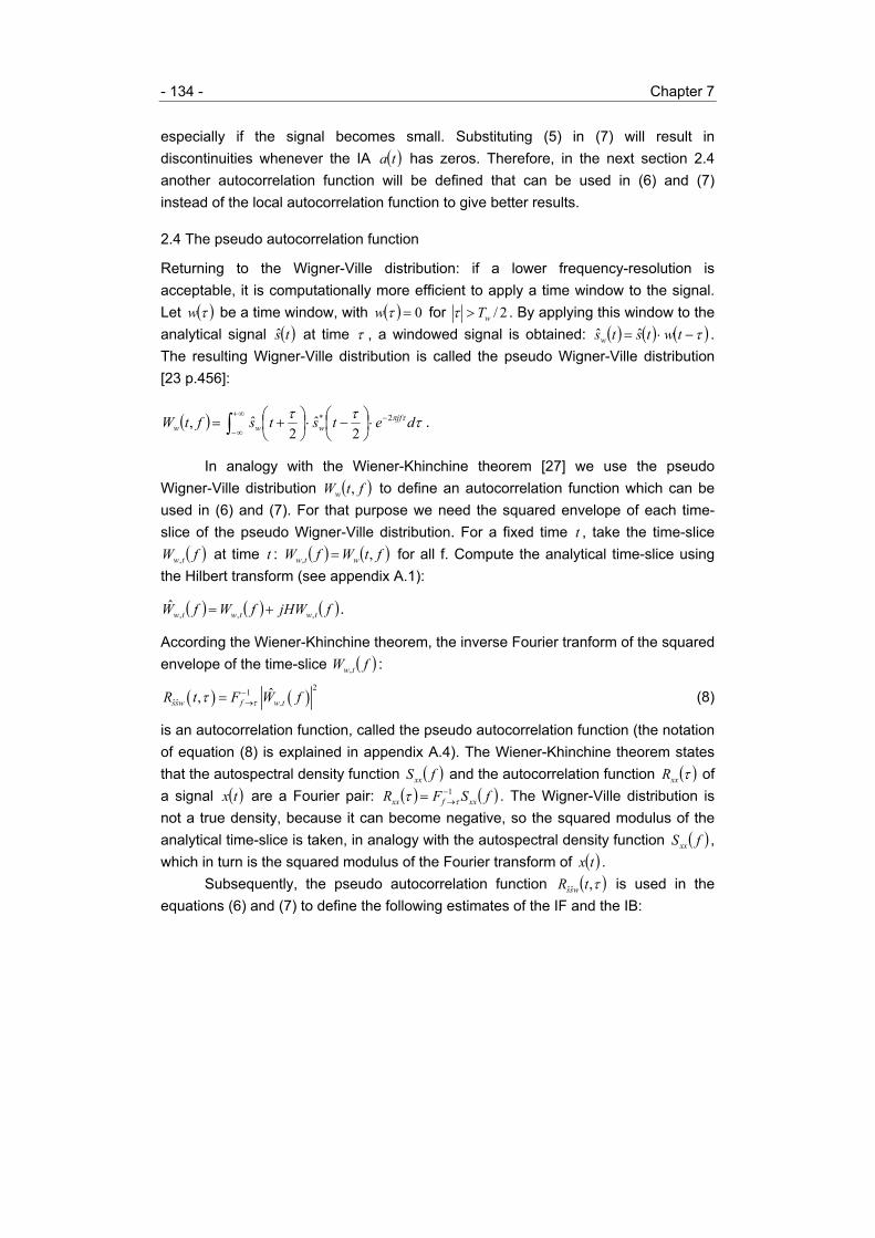
- 134 - Chapter 7
especially if the signal becomes small. Substituting (5) in (7) will result indiscontinuities whenever the IA ( )ta has zeros. Therefore, in the next section 2.4another autocorrelation function will be defined that can be used in (6) and (7)instead of the local autocorrelation function to give better results.
2.4 The pseudo autocorrelation function
Returning to the Wigner-Ville distribution: if a lower frequency-resolution isacceptable, it is computationally more efficient to apply a time window to the signal.Let ( )τw be a time window, with ( ) 0=τw for 2/wT>τ . By applying this window to theanalytical signal ( )ts at time τ , a windowed signal is obtained: ( ) ( ) ( )τ−⋅= twtstsw ˆˆ .The resulting Wigner-Ville distribution is called the pseudo Wigner-Ville distribution[23 p.456]:
( ) ∫∞+
∞−
−⋅
−⋅
+= τττ τπ detstsftW jf
www2*
2ˆ
2ˆ, .
In analogy with the Wiener-Khinchine theorem [27] we use the pseudoWigner-Ville distribution ( )ftWw , to define an autocorrelation function which can beused in (6) and (7). For that purpose we need the squared envelope of each time-slice of the pseudo Wigner-Ville distribution. For a fixed time t , take the time-slice
( )fW tw, at time t : ( ) ( )ftWfW wtw ,, = for all f. Compute the analytical time-slice usingthe Hilbert transform (see appendix A.1):
( ) ( ) ( )fjHWfWfW twtwtw ,,,ˆ += .
According the Wiener-Khinchine theorem, the inverse Fourier tranform of the squaredenvelope of the time-slice ( )fW tw, :
( ) ( )21
ˆˆ ,ˆ,ssw f w tR t F W fττ −
→= (8)
is an autocorrelation function, called the pseudo autocorrelation function (the notationof equation (8) is explained in appendix A.4). The Wiener-Khinchine theorem statesthat the autospectral density function ( )fSxx and the autocorrelation function ( )τxxR ofa signal ( )tx are a Fourier pair: ( ) ( )fSFR xxfxx
1−→= ττ . The Wigner-Ville distribution is
not a true density, because it can become negative, so the squared modulus of theanalytical time-slice is taken, in analogy with the autospectral density function ( )fSxx ,which in turn is the squared modulus of the Fourier transform of ( )tx .
Subsequently, the pseudo autocorrelation function ( )τ,ˆˆ tR wss is used in theequations (6) and (7) to define the following estimates of the IF and the IB:

Instantaneous amplitude and frequency - 135 -
( ) ( )1,arg21
ˆˆ tRtf wssw π= , (9)
( ) ( )( )
ˆˆ22
ˆˆ
,11 1,0
ssww
ssw
R tB t
R tπ
= −
. (10)
Due to the applied window, the pseudo autocorrelation function ( )τ,ˆˆ tR wss is not aninstantaneous value and therefore (9) and (10) are not instantaneous measures: theyare ‘local estimators of the instantaneous frequency and the instantaneousbandwidth’. The ‘smoothing’ effect of the window is apparent. The use of a windowedsignal diminishes the effect of noise and stabilizes ( )tfw . However, under certainconditions imposed on the signal and the time window, the estimates will beinstantaneous. Sections 3.2, 3.3, and 3.4 describe the combination of a band-passfilter, which is used to make the signal band-limited, and a time window chosenaccording to the uncertainty principle of Gabor, which will make ( )τ,ˆˆ tR wss
instantaneous. Using this instantaneous pseudo autocorrelation function, theestimates ( )tfw and ( )wB t are well-behaving instantaneous measures of the IF andIB.
3 Method
Under certain assumptions, the theory of section 2 can be applied to heart ratevariability. Our model signal is a band-limited, monocomponent, and analytical signal.It is expected that on the basis of this model the time-varying IA, IF, and IB can bederived accurately, because the model signal corresponds sufficiently to thequadrature model signal (see appendix A.1).First, the design of the zero-phase band-pass FIR-filters is described in the nextsection 3.2. These filters correspond to the mid- and high-frequency ranges ofinterest as mentioned in the Introduction. Then a time window has to be selectedaccording to the uncertainty principle of Gabor to compute the pseudo Wigner-Villedistribution. The length of this time window is dependent on the bandwidth of theapplied filter. This is described in sections 3.2, 3.3, and 3.4. After that we have tosequentially perform the following steps to compute the estimates of the IA, IF, andIB:• Compute an equidistantly sampled heart rate variability time series from thedetected R-waves in the electrocardiogram (section 3.1).• Decompose the heart rate variability time series into narrow-band mid- and high-frequency components by zero-phase band-pass FIR-filtering.

- 136 - Chapter 7
• The analytical signal is computed by means of a Hilbert transform FIR-filter (seeappendix A.2).• This yields the IAs for the narrow-band mid- and high-frequency components.• The pseudo Wigner-Ville distribution is computed, using a time window asdescribed in sections 3.2, 3.3, and 3.4.• The time-slices of the pseudo Wigner-Ville distribution are made analytical bymeans of the Hilbert transform based on the discrete Fourier transform (see appendixA.1).• And the discrete inverse Fourier transform of the squared envelope of each time-slice is used to compute the pseudo autocorrelation function.• The final step is to derive the estimates of the IF and the IB for each of thenarrow-band components from the pseudo autocorrelation function (section 3.5).
3.1 The computation of an equidistantly sampled analytical heart rate variability timeseries
Heart rate variability time series are obtained by detecting the R-waves from theelectrocardiogram with a resolution of 1 ms and subsequently generating a pulsetrain consisting of Dirac pulses at the R-wave occurrence times. This pulse train isdemodulated by means of a low-pass filter with cutoff frequency of 0.5 Hz [32,33].The output signal of the filter is called the ‘low-pass filtered cardiac event series’, andcan be sampled regularly [33,34,35]. In our case, the filtered event series is sampledwith a sample interval 0.25st = sec, i.e., the sample frequency is 1 4s sF t= = Hz. Theresulting discrete real heart rate variability time series is denoted by[ ] , 0,..., 1s n n N= − .
The time series [ ]s n is filtered with a zero-phase band-pass FIR-filtercorresponding to one of the frequency ranges of interest, i.e., mid- or high-range. Thefiltered time series is subsequently filtered with a zero-phase Hilbert transform FIR-filter to obtain the analytical time series (see appendix A.1). The resulting analytical,band-limited, and monocomponent time series is denoted by [ ]ˆ , 0,..., 1s n n N= − .Each complex number [ ]s n can be presented in polar form: [ ] [ ] [ ]ˆ j ns n a n e ϕ= , withnon-negative envelope or IA [ ]a n and IP [ ]nϕ .
3.2 Filter bandwidth and duration of the impulse response according to Gabor
We designed the band-pass filters for the mid- and high-frequency components of theHRV-signal based on the requirements of an optimal resolution in the time-domain,unity-gain, and a minimal overlap between consecutive band-pass filters.

Instantaneous amplitude and frequency - 137 -
To find the best possible resolution in time, we started from the uncertaintyprinciple of Gabor [20]. Gabor stated that, for a given filter, the product of the width inthe time-domain and the width in the frequency-domain is greater than or equal to1 4π . In equation:
14t fσ σπ
⋅ ≥ (11)
This means that, the wider (or narrower) the bandwidth of a filter is, the shorter (orlonger) the corresponding impulse response is in the time-domain. The minimalproduct in the above equation (11) is reached for a normal distribution, that is aGaussian shaped filter. Any other filter shape will deviate from a minimal product in(11).
In the above equation, tσ and fσ are expressed in a statistical sense todescribe the width of a distribution as the second moment – or the standard deviation– of such a distribution:
( ) 22 21t t h t dt
Eσ
+∞
−∞= ⋅∫ (12)
and
( ) 22 21f f H f dfE
σ+∞
−∞= ⋅∫ (13)
where ( )H f constitutes the filter transfer function in the frequency domain and ( )h tits corresponding impulse response in the time domain. E is the power of both ( )h tand ( )H f :
E = ( ) 2h t dt+∞
−∞∫ = ( ) 2H f df+∞
−∞∫ .
Note that the expressions (12) and (13) are invariant for the localization of the filteron the frequency axis. So, for a given low-pass filter, the same product t fσ σ⋅ holdstrue if this low-pass filter is translated over the frequency axis.
In the case of band-pass filters for the mid- and high-frequency components ofthe HRV-signal, the width in the frequency-domain is defined by the characteristicfrequency ranges of HRV. The corresponding width in the time-domain then isdetermined by the duration of the impulse response expressed in terms of itsstandard deviation. On its turn, this standard deviation yields a measure for theresolution in time, i.e., spacing of points in time that are statistically independent; thiswill be explained below.
Long-tailed Gaussian shaped filters are incompatible with the unity-gainrequirement. To be as close as possible to Gabor’s optimum, we used ‘squaredcosine shaped’ filters instead. Because in our case consecutive filters have a wider

- 138 - Chapter 7
bandwidth, the slopes of the filters need to be asymmetrical. The trailing slope istwice the length of the leading slope, but the trailing and leading slope of consecutiveband-pass filters are equal (see figure 1); this yields the desired unity-gain filter-bank.A discrete zero-phase band-pass FIR-filter is designed by defining the cutofffrequencies (in our case the –6 dB points) 1cf and 2cf , and the transition bands[ ]1 1,b tf f and [ ]2 2,t bf f (see figure 2). The pass-band is the interval [ ]1 2,c cf f betweenthe cutoff frequencies. The filter-basis is the interval [ ]1 2,b bf f , i.e. the pass-band plusthe two transition bands. The center frequency is the midpoint of the base:
( )0 1 2 / 2b bf f f= + .
We computed the product of tσ and fσ for the squared cosine shaped mid-en high-range band-pass filters and compared this product to the minimal product ofGabor’s Gaussian shaped filter. For the mid-range filter:
4.6512tσ = sec, 0.0204fσ = Hz, and 1.19 4t fσ σ π⋅ = (14)
For the high-range filter:
1.3960tσ = sec, 0.0952fσ = Hz, and 1.67 4t fσ σ π⋅ = (15)
The replacement of Gaussian shaped filters by squared cosine shaped filters toaccomplish unity gain has only a small impact on the product of width in frequency-and time-domain, and is close to optimal.
1bf 2cf0f 2tf1cf 1tf 2bf
1.0
0.5
( )H f
2n sF F=
Figure 1. The set of consecutive band-pass filters for the low-, mid-, and high-frequency components constitutes a unity-gain filter-bank. The slopes are ‘squaredcosine shaped’.

Instantaneous amplitude and frequency - 139 -
LOW MID HIGH 2sF
1.0
0.5
( )H f
Figure 2. The design of a band-pass FIR-filter. The pass-band is the frequencyinterval [ ]1 2,c cf f , defined by the two cutoff frequencies, in our case –6 dB points,
1cf and 2cf . The filter-basis is the interval [ ]1 2,b bf f . The two transition bands[ ]1 1,b tf f and [ ]2 2,t bf f , are ‘squared cosine shaped’ slopes. The trailing slope ismade twice as long as of the leading slope. The center frequency 0f is themidpoint of the basis: ( )0 1 2 / 2b bf f f= + . The signal to be filtered is analytical,therefore there is no pass-band at the negative frequencies.
1.0
2b nf f′ =1bf ′
( )H f
0.5
1cf ′ 2cf ′2tf ′1tf ′
Figure 3. The filter-basis of the band-pass filter of figure 2 is translated over arange 0f towards the origin. This basis of this filter lies symmetrical around thezero frequency. After demodulation of the signal with frequency 0f , it is sufficientto sample the filtered signal with sample rate 22 bf ′⋅ .

- 140 - Chapter 7
3.3 Low-pass equivalent and dependency between adjacent points in time
The center frequency of a given band-filter is the midpoint of the base:( )0 1 2 / 2b bf f f= + . Suppose we translate the frequency response of the filter towards
the zero frequency over a range 0f . It follows that: 1bf ′ = 1 0bf f− = 2 0bf f− + = 2bf ′− ,i.e., the basis of this filter lies symmetrical around the zero frequency (figure 3).Therefore, after demodulation of the signal with frequency 0f , it is sufficient tosample the filtered signal with sample rate 22 bf ′⋅ [27]. This means that, in case of anideal rectangular band-pass filter, the application of the translated low-pass filter incombination with complex demodulation will result in an over-sampled demodulatedsignal and the ‘over-sampling ratio’ is:
DF2 1
s
b b
Fnf f
=−
.
In fact, we could decimate or downsample the time series with a ‘decimation factor’
DFn and still retain the same information. In this downsampled situation, the adjacentpoints in time are uncorrelated, so independent in a statistical sense. That meansthat parameters computed at this resolution then are instantaneous. In that case theamplitude and the frequency are called instantaneous amplitude and frequency.Computations over a shorter time-interval yield adjacently dependent points in time; ifcomputed over a longer time-interval, properties will be averaged, i.e., smeared overtime (as with Fourier analysis). The decimation factor DFn depends on the samplefrequency sF and the width of the filter at the basis. In our case of a 4 Hz sampledHRV time series and our design of the band-pass filters, the decimation factor for themid-range filter is 31, and the decimation factor for the high-range filter is 9.
However, instead of downsampling, we utilize all the original DFn points withina window to compute a pseudo Wigner-Ville ‘time-slice’ (see sections 2.4 and 3.5)and this is repeated for all the adjacent and disjoint intervals of DFn points. Hence theconsecutive time-slices of the pseudo Wigner-Ville distribution will be independent.This will make the pseudo autocorrelation function ( )τ,ˆˆ tR wss and consequently theestimates of the IF and the IB also instantaneous. This design of the time-window willbe used in the following section 3.5. However, to provide smooth IF and IB timeseries, we shift the window of DFn points point by point.
In our case, we do not use rectangular band-pass filters, but band-pass filterswith squared cosine shaped transition bands to achieve smoother time-domainbehavior according to Gabor. This means that, using the same window length DFnthat we derived for the rectangular filter, the consecutive time-slices of the pseudoWigner-Ville distribution are not truly independent. But the consequential dependency

Instantaneous amplitude and frequency - 141 -
of consecutive estimates of the IF and the IB is minimal; and therefore we claim thatwe can consider the estimates of the IF and the IB to be instantaneous.
3.4 Time-resolution and instantaneous properties of mid- and high-frequencycomponents
To investigate the maximal discrete resolution t∆ in time that we can accomplish withthe postulated asymmetrical band-pass filters, we computed the envelope ( )h t ofthe impulse response ( )h t of the demodulated band-pass filter ( )0H f f− , i.e., ( )h tis the inverse Fourier transform of the frequency response ( )0H f f− . The frequencyresponse ( )0H f f− is the low-pass analogy of the band-pass filter afterdemodulation with 0f . The frequency 0f is the center frequency of the band-passfilter (see sections 3.2 and 3.3). In case of the mid-range band-pass filter, the centerfrequency is 0 0.1230f = Hz. To determine the discrete instantaneous value t∆ in thetime domain, the Nyquist frequency of the demodulated band-pass filter wasdetermined to be
22s
n bDF
Ff fn
′= =
(section 3.3 and figure 3), i.e., 2 31 0.0645nf = = Hz, to allow for perfect signalintegrity, whilst minimizing sidelobes in the filter impulse response and thereforedependency between adjacent points in time. The numerical values of ( )h t around0t = are:
( )0.03 0.05 0.26 0.58 0 0.26 0.05 0.03t = (16)
with 7.75t∆ = sec (= 31 samples) (17)
and 1.6662 tt σ∆ =
(see equation (14)). These results mean the following. If, after filtering with the mid-range band-pass filter, consecutive Wigner-Ville time-slices are computed over
7.75t∆ = sec (= 31 samples), these consecutive time-slices and the computedestimates of IF and IB are not truly independent, so not truly instantaneous. They stillshow a minimal dependency over (mainly) 3 data points as given by (16).
In case of the high-range band-pass filter, 0 0.3447f = Hz, 2 9 0.2222nf = =Hz, and the numerical values of ( )h t around 0t = are:
( )0.05 0.12 0.21 0.75 0 0.21 0.12 0.05t = (18)

- 142 - Chapter 7
with 2.25t∆ = sec (= 9 samples) (19)
and 1.6117 tt σ∆ =
(see equation (15)). Also in this case there is a dependency over (mainly) 5 datapoints as given by (18).
For the remainder of this article, ‘instantaneous’ is referred to as consecutivepoints in time only showing a minimal dependency in time as given by (16) and (18)and spaced over t∆ as given by (17) and (19) for the mid- and high-range band-passfilter, respectively.
3.5 The discrete pseudo autocorrelation function
Let [ ]ˆ , 0,..., 1s n n N= − be a filtered analytical heart rate variability time series, i.e.,mid- or high-range. A real-valued discrete time window [ ] 1,...,0, −= Miiw of length
DFM n= is chosen. Conform sections 3.3 and 3.4, this length is chosen to make theestimates of the IF and the IB instantaneous. The discrete pseudo Wigner-Villedistribution is defined by [23 p.456]:
[ ] [ ] [ ] [ ] [ ]∑−=
⋅−⋅−+=1
1
/4** ˆˆ,M
Mi
Mikjw einsiwinsiwknW π , (20)
with 1 2M M= , for 1,...,0 −= Nn and 1,...,0 −= Mk . We use the algorithm ofBoashash and Reilly [36] to compute the discrete pseudo Wigner-Ville distribution.
The next step is the computation of the discrete pseudo autocorrelationfunction (DPACF). For each time index n take the time-slice [ ] [ ]knWkW wnw ,, = , for
1,...,0 −= Mk , of the discrete pseudo Wigner-Ville distribution [ ],wW n k . This is a realdata series in the frequency domain. Since the discrete pseudo Wigner-Villedistribution also contains negative values (it is not a true density), we will start todetermine the squared envelope of each time-slice. To accomplish this, compute thediscrete analytical data series:
[ ] [ ] [ ]kjHWkWkW nwnwnw ,,,ˆ += .
This method constitutes in fact a band-pass filtering of the positive times and azeroing of the negative times (see appendix A.1 and A.2). After that, the squaredmodulus of the analytical time-slice is taken to yield the squared envelope of thetime-slice. The procedure of computing the envelope of the time-slice can be seen asa smearing function of this data series in the frequency domain. It follows that theinverse Fourier transform of the envelope constitutes a particular real weighting

Instantaneous amplitude and frequency - 143 -
function in the τ -domain, with a maximum value at 0=τ . We now compute theinverse discrete Fourier transform of the squared envelope of the time-slice [ ],w nW k ,in the index k :
[ ] [ ]21
ˆˆ ,ˆ,ssw k l w nR n l F W k−
→= , for 1,...,0 −= Ml . (21)
(See appendix A.4). The resultant [ ]lnR wss ,ˆˆ is called the DPACF. (Equation (21)corresponds with equation (8) of section 2.4.)
The computation of the discrete estimator [ ]nfw of the IF and the squaredestimator [ ]2
wB n of the IB are now straightforward using the expressions:
[ ] [ ][ ]
⋅=
1,Re1,Imarctan
22/
ˆˆ
ˆˆ
nRnRFnf
wss
wsssw π
(22)
and
[ ] [ ][ ]0,1,
1ˆˆ
ˆˆ2
nRnR
nBwss
wssw −= , (23)
corresponding with equations (9) and (10). These estimates are instantaneousconform section 3.4. Concerning equation (22), the value [ ]ˆˆ ,1sswR n is an estimate ofthe local autocorrelation function ( )ˆˆ ,sslR t τ at 1τ = , therefore, phase-shifts of 2π± dueto the ambiguity of the inverse tangent do not occur, as explained in section 2.3, andunwrapping is not necessary. Concerning equation (23), zero divisions cannot occurbecause the maximum of the series [ ]ˆˆ , , 0,..., 1sswR n l l M= − is at 0l = , and this dataseries can only be identical to zero if the time series [ ]ns is locally identical to zero(see section 2.3).
At this point it is recalled that the DPACF [ ]lnR wss ,ˆˆ is weighted or multipliedwith a real weighting function that resulted from the calculation of the envelope of thetime-slice in the frequency domain. Because [ ]lnR wss ,ˆˆ has been weighted, [ ]nBw
2 is abiased squared estimator of the (squared) IB. The index [ ]nBw
2 , however, is useful asan indicator of noise or interference due to other signal components. Therefore, thisindex is called the instantaneous bandwidth coefficient (IBC). The IBC [ ]nBw
2 is aqualitative index and is chosen in such a way that it will always have a value between0 and 1 (note the absence of the factor 21 π in equation (23), e.g., equation (10)).Value 0 means that there is no amplitude modulation, so the signal is purelyfrequency modulated (see section 2.2); value 1 means that the signal is a noisesignal. The estimator [ ]nfw is useful to calculate the IF and is not biased because

- 144 - Chapter 7
both real and imaginary part of [ ]1,ˆˆ nR wss have been multiplied by the same real factorof the weighting function.
3.6 The circular mean direction
Finally, we describe the computation of the circular mean direction. The circularmean direction is an estimate of the IF. In the next section 4, we make a comparisonbetween this estimate and our estimate of the IF.Again, let [ ]ˆ , 0,..., 1s n n N= − be a filtered analytical heart rate variability time series.A real-valued discrete time window [ ] 1,...,0, −= Miiw , is chosen. This window maybe relatively long, for instance 100M = . The discrete pseudo Wigner-Ville distribution
[ ],wW n k is computed using equation (20). The discrete first moment [37]:
[ ][ ]
[ ]∑
∑−
=
−
=
⋅⋅= 1
0
1
0
,
,M
kw
M
kw
si
knW
knWk
MFnf
is an estimate of the IF, corresponding with equation (2). However, the discretepseudo Wigner-Ville distribution is periodical, therefore this estimate is biased [23p.463]. A better estimate is the circular mean direction [23,38,39]:
[ ] [ ]∑−
=
⋅⋅⋅=1
0
/2,arg22/ M
k
Mkjw
si eknWFnf π
π, (24)
which takes the periodical character of the data into account.The estimation of the discrete IB using the discrete second moment, correspondingwith equation (3), as well as using the circular standard deviation [38], givesunsatisfactory results, see also section 2.2.
4 Application and discussion
4.1 Mid- and high frequency components, the IA
Figure 4 presents an illustration of the application of the method to a heart ratevariability time series in the mid-frequency range (0.07-0.15 Hz) and the high-frequency range (0.15-0.50 Hz). The upper graph of A is an example of a heart ratevariability time series, sampled with 4 Hz. The result of the mid-range filter applied tothe heart rate variability time series is shown in B (mf), and the result of the high-range filter is shown in E (hf). The result of a combined (zero-phase) MID+HIGH-range FIR-filter (0.07-0.50 Hz) is shown in the lower graph of A (mf&hf). Adding themid- and the high-frequency heart rate variability time series in B and E, respectively,

Instantaneous amplitude and frequency - 145 -
results in exactly the same MID+HIGH-frequency heart rate variability time series.This is the case because the FIR-filters are zero-phase and have compensatingoverlap in the transition bands, i.e., they constitute a unity-gain filter-bank (section3.2).
The envelope or IA of the mid-frequency heart rate variability time series ispresented in B. It is apparent that the IA is fluctuating slowly with respect to the mid-frequency heart rate variability time series. This is in agreement with the conditionsmentioned in section 2.1. (I.e., to be able to compute a meaningful IF, the spectra ofthe envelope and the phase have to be disjoint, whereby the envelope has to belower in frequency than the phase; see also conditions 1) and 2) of appendix A.1.)The same applies to the IA of the high-frequency heart rate variability time series inE.
4.2 The IF and the IBC
Figure C shows the estimators [ ]nfw of the IF and [ ]nBw2 of the IBC of the mid-
frequency heart rate variability time series in B. Notice the instants in time where theIBC is high. These high values correspond with:a) low, almost zero, values of the IA in B;b) phase-shifts of the mid-frequency heart rate variability time series, see B;c) irregularities in the IF in this figure (some peaks are deflected); andd) fast changes in the circular mean direction in figure D.At these points of high valued IBC, the signal may not fulfill the requirements of ourmodel signal. This means that locally the signal may not be monocomponent,causing phase-shifts at low amplitudes. Or the high values may be due to randomphase-shifts. This will be explained below by adding two sinusoids. The sameremarks can be made with respect to the estimators [ ]nfw of the IF and [ ]nBw
2 of theIBC, presented in figure F, of the high-frequency heart rate variability time series in E.
Figure D shows the discrete IF of the mid-frequency heart rate variability timeseries, estimated with the circular mean direction (24). Notice the peaks that stretchout of the mid-frequency range and some peaks even become negative. Theestimation of the accessory discrete IB using the discrete second moment,corresponding with equation (3), as well as using the circular standard deviation [38],give unsatisfactory results, as mentioned in section 3.6, making these methodsunsuitable for practical use. As mentioned in section 2.1, the estimate of the IF of amulticomponent signal can shift out of the signal’s spectral region, and this is whatwe see in figure D. Notice the resemblance of the circular mean direction in D andthe IF in C. Except for the periods of high IBC, these two estimators are almost equal
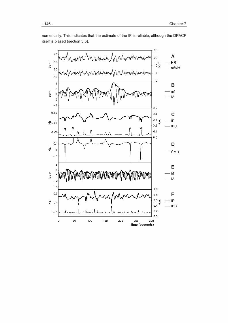
- 146 - Chapter 7
numerically. This indicates that the estimate of the IF is reliable, although the DPACFitself is biased (section 3.5).

Instantaneous amplitude and frequency - 147 -
4.3 The behavior of the IF and the IBC
The irregularities in the IF at points of high valued IBC, 1) when the signal is locally,i.e., for a short period in time, not monocomponent, or, 2) due to random phasefluctuations in the original signal, may be explained as follows.1) A signal is locally multicomponent ([16,18,21,23], see also appendix A.3) in thefrequency band of interest if there is locally more than one spectral concentrationpresent in the time-varying ‘instantaneous spectrum’. For instance, a signal maylocally become multicomponent if harmonic or sub-harmonic components arise dueto non-sinusoidal shape of waveforms. For multicomponent signals, the IF has no
Figure 4. Spontaneous fluctuations in heart rate and the estimated instantaneousamplitude, frequency, and bandwidth coefficient of the MID and HIGH frequencybands, during a period of 300 sec.A: The upper graph presents the original unfiltered 4 Hz heart rate time series(HR), the scale in beats per minute (bpm) is on the left side. The lower graph(mf&hf) is the result the combined MID+HIGH filter applied to the heart rate. Thescale in bpm is on the right side.B: The thin line (mf) presents the MID frequency HR time series. The bold line (IA)is the instantaneous amplitude or envelope of this time series. Both graphs arescaled in bpm.C: The estimated instantaneous frequency (IF, upper bold graph) and theinstantaneous bandwidth coefficient (IBC, lower thin graph) of the MID frequencyHR time series as presented in B. The scale of the IF in Hz is on the left side, thescale of the IBC in arbitrary units (a.u.) is on the right side.D: The instantaneous frequency (CMD) estimated by means of the circular meandirection, of the same MID frequency HR time series as presented in B. The scaleis in Hz.E: The thin line (hf) presents the HIGH frequency HR time series. The bold line(IA) is the instantaneous amplitude of this time series. Both graphs are scaled inbpm.F: The estimated instantaneous frequency (IF, upper bold graph, scale in Hz onthe left side) and the instantaneous bandwidth coefficient (IBC, lower thin graph,scale in a.u. on the right side) of the HIGH frequency HR time series as presentedin E.

- 148 - Chapter 7
meaning [21]. The effect is that phase-shifts at low amplitudes cause discontinuitiesin the IF and the IBC. For instance, suppose ( )ts consists of two sinusoids withdifferent frequencies 2 1f f> [39]:
( ) ( ) ( )( )d1 2 2 sign cos 2 f2 2ˆ 2 cos 2 hjf t j tjf t jf tds t e e f t e π π ππ π π + ⋅= + =
in which ( )2 1 2df f f= − and ( )1 2 2hf f f= + . The signal ( )ts is a complex analyticalsignal and the IA is ( ) ( )2 cos 2 da t f tπ= . The double sinusoid shows phase-shifts of2π± at each time the cosine function ( )cos 2 df tπ of the IA changes sign. Phase-shifts
cause discontinuities in the IF, because the IF is the derivative (1) of the phase. Itfollows from equation (4) that the IBC is approximated by:
( ) ( )2 2 2 2tan 2i d dB t f f tπ π= .
Therefore, there are high peaks in the IBC at times where the cosine function( )cos 2 df tπ changes sign. The deflections in the IF and the IBC are due to aliasing
because the sample frequency is too low to catch the slope of the peaks.2) Random phase fluctuations may have various origins. It may be quantization noisedue to small R-wave detection errors. It may also be physiological noise originatingfrom stochastic components of the underlying physiological system. Under pure noiseconditions, neighbouring samples in time are uncorrelated. If noise is present on thesignal, this may result in ‘sudden’ phase-shifts. ‘Sudden’ phase-shifts, in turn, mayresult in discontinuities in the IF, as explained above. Also, the autocorrelationfunction at 1τ = of a noisy signal is zero in expectation, but varies randomly.Therefore, the IBC (7,23) of a noisy signal varies randomly and will show outlierpeaks. By nature, the IBC is peaked at all phase-shifts. Deflections in IF and IBCoriginate in the same way as explained in 1), see figures C and F.
5 Conclusion
In this paper, we have provided methods to compute estimators of the instantaneousamplitude, frequency, and bandwidth coefficient of certain narrow-band componentspresent within heart rate variability time series; these components are separatedusing predefined zero-phase band-pass FIR-filters. The estimators offer aquantitative description of the time-varying spectral energy of the heart rate variabilitysignal within each frequency band. At every instant in time, the IA offers an estimateof the signal’s instantaneous power, while the IF estimates the time-varyingfrequency location of the spectral peak. Together they provide a time-frequencydescription of the energy in a particular frequency band. A comparison with the

Instantaneous amplitude and frequency - 149 -
circular mean direction gives an indication of the reliability of the estimate of the IFcomputed with our method.
The IBC may serve as a time-dependent indicator of oscillatory and irregularperiods. Oscillatory fragments with low IBC can be used in further analysis, irregularfragments of high IBC can be excluded or otherwise processed.
At periods of high IBC, the interaction of other signal components may beinvestigated, for instance with cross-correlation techniques. In addition, the IF in bothmid- and high-frequency band may show possible harmonic relationships at thoseperiods in time where the components are coupled by phase locking. A non-sinusoidal waveform in the mid-frequency band may show a clear harmoniccomponent in the high-frequency band. Otherwise, respiration components mayproduce sub-harmonic components in the mid-frequency band. Phase locking maybe revealed by means of cross-correlation.
The traditional approach of short-term Fourier spectral analysis is based ontime windows of 2-5 min to yield an appropriate frequency-resolution. The resolutionin time of the described method is in the order of several seconds, inversely relatedto the width of the band-pass filter. This optimal resolution in time reveals the highlydynamic nature of the various components in the heart rate, comprising the,sometimes antagonistic, waxing and waning in time of the mid- and high-frequencycomponents. This dynamic behavior is smeared over time and thus hidden whenusing traditional time-averaged spectral analysis techniques.
The presented method provides instantaneous information of time-varyingchanges in heart rate variability, with an optimal time-resolution. Therefore, thismethod may contribute to a more detailed description of the time-varying dynamics ofthe autonomic regulatory processes within the cardiovascular control system undernormal or pathological conditions.
Appendix
A.1 Analytical signals
Given a complex signal ( )tz , the envelope or instantaneous amplitude ( )ta and theinstantaneous phase ( )tϕ are defined as the modulus and the argument of thecomplex number ( )tz . The signal ( )tz can subsequently be written in polar form( ) ( ) ( )tjetatz ϕ= and visualized as a moving vector in the complex plane. Furthermore,
the instantaneous frequency ( )tfi may now be defined as the rate of change of thephase: ( ) ( ) 2if t tϕ π′= . To compute the instantaneous amplitude, phase, and

- 150 - Chapter 7
frequency of a real signal, we need a complex representation that represents the realsignal in a ‘natural’ way.
There is a unique way to represent a simple harmonic oscillation( ) tats ωcos⋅= as a rotating vector in the complex plane. Namely, by adding the
imaginary quadrature component ( ) tjatjQs ωsin⋅= . The resulting complex vector is( ) tjeatz ω⋅= . More generally, the natural complex representation of ( ) ( ) ( )ttats ϕcos=
as a complex vector is ( ) ( ) ( )tjetatz ϕ= , in which the imaginary quadrature componentis ( ) ( ) ( )ttjatjQs ϕsin= [20].
Constructing a unique natural complex representation of a real signal ( )ts byfirst writing the real signal in the form ( ) ( ) ( )ttats ϕcos= and subsequently adding theimaginary quadrature component is called the quadrature operation. The real signalis represented as a moving vector in the complex plane and the real part of thecomplex signal is equal to the original real signal. The resulting complex signal iscalled the quadrature model signal. The quadrature model signal is assumed to bethe natural complex representation of a real signal and the instantaneous amplitude( )ta and phase ( )tϕ represent the instantaneous amplitude and phase of the original
real signal [21 p.36].In that respect, one needs the quadrature model signal of a real signal to be
able to compute the instantaneous amplitude and phase of this signal. However,there is no unique way to write a real signal ( )ts in the form ( ) ( ) ( )ttats ϕcos= , and sothere is no unique way to construct a complex representation of a general real signalby means of the quadature operation [16,21].
To overcome this problem, Gabor [20] introduced the analytical signal of a realsignal ( )ts . The construction is as follows. Another real signal ( )Hs t is constructed byreplacing each component cosa tω⋅ of ( )ts with sina tω⋅ and each componentsinb tω⋅ with cosb tω− ⋅ . Consequently, the complex signal
( ) ( ) ( )s t s t jHs t= +
consists of components j ta e ω⋅ (replacing each component cosa tω⋅ ) andcomponents j tjb e ω− ⋅ (replacing each component sinb tω⋅ ). This signal ( )s t is calledthe analytical signal. The real signal ( )Hs t is called the Hilbert transform of ( )ts . Itfollows that ( )Hs t can be considered as the output of a filter with frequency response
( )H f defined by ( ) 1H f = for 0f > ; ( )0 0H = ; and ( ) 1H f = − for 0f < [27]. In thetime domain, the impulse response of ( )H f is
( ) ( )1 1f th t F H f tπ−→= =

Instantaneous amplitude and frequency - 151 -
and the Hilbert transform is the convolution ( ) ( )s t h t∗ . The mathematical form of theHilbert transform is
( ) ( )( )
. .s
Hs t p v dtτ
τπ τ
+∞
−∞=
−∫
[20,21,27]. (P.v. means that Cauchy’s principle value of the integral has to be taken.)The resulting analytical signal is a complex signal and has two properties:a) The amplitudes of the positive frequency components of the analytical signalequal the amplitudes of the positive frequency components of the original real signalmultiplied by two, but the negative frequency components are eliminated; andb) the real part of the complex analytical signal equals the real signal.With respect to these two properties, the construction of the analytical signal of a realsignal is unique [16 p.523].
The analytical signal is meaningful if it is equal to, or an approximation of, thequadrature model signal because then the instantaneous amplitude and phase aremeaningful, as explained above. However, the analytical signal is not always equal tothe quadrature model signal. If there is a leakage of positive frequency componentsinto the negative spectral region, then the analytical signal will not correspond to thequadrature model signal, because the Hilbert transform eliminates the negativefrequency components.
Consider the real signal ( ) ( ) ( )coss t a t tϕ= . Suppose:1) the spectrum of ( )ta is contained in a frequency region 11 ωωω <<− ; and2) the spectrum of ( )tϕcos is zero for 1 1ω ω ω− ≤ ≤ .Under these conditions, it can be proved that
( ) ( ) ( ) ( )cos cosa t t jH a t tϕ ϕ+ = ( ) ( )j ta t e ϕ ,
meaning that the analytical signal and the quadrature model signal coincide [16,21].Therefore, the analytical signal ( ) ( ) ( )ˆ j ts t a t e ϕ= of a real signal ( )ts equals thequadrature model signal, if ( )ta and ( )tϕ satisfies 1) and 2), i.e., under theseconditions, the instantaneous amplitude and phase are meaningful. In general, for anarrow-band real signal, the analytical signal approximates the quadrature modelsignal because there is little or no leakage of the positive frequency components intothe negative spectral region.
Under the same conditions 1) and 2), reflecting a slowly varying amplitudemodulation and a fast phase modulation, the instantaneous amplitude ( )ta and theinstantaneous phase ( )tϕ can be treated as independent signals [16]. Furthermore,

- 152 - Chapter 7
Rihaczek [22] proved that the time-varying signal’s energy is in frequencyconcentrated in a single narrow frequency range at ( )tff i= .
A.2 Discrete analytical time series
Based on the above description, there are two methods to compute the discreteanalytical signal:1) Use the fact that the negative frequency components must be zero and thepositive frequency components are twice the positive frequency components of theoriginal real signal. Let [ ] 1,...,0, −= Niix be a discrete time series and[ ] 1,...,0, −= NkkX the discrete Fourier transform of [ ]ix . For N is odd, define
2/NM = and [ ] [ ]00ˆ XX = , [ ] [ ]kXkX ⋅= 2ˆ for Mk ≤≤1 , and [ ] 0=kX for11 −≤≤+ NkM . For N is even, define ( ) 12/ −= NM and [ ] [ ]00ˆ XX = , [ ] [ ]kXkX ⋅= 2ˆ
for Mk ≤≤1 , [ ] [ ]2/2/ˆ NXNX = , and [ ] 0=kX for 12 −≤≤+ NkM . The inversediscrete Fourier transform of [ ]kX produces the discrete analytical signal[ ] 1,...,0,ˆ −= Niix [23 p.458].
2) In the time domain, the discrete impulse response of the Hilbert transform ( )H fcan be used to filter the real signal [ ] , 0,...,x i i L= to obtain the imaginary part of thediscrete analytical signal [36,40]. The discrete frequency response
[ ], / 2,..., / 2H k k N N= − is defined by [ ] 1H k = − for 0k < ; [ ]0 0H = ; and [ ] 1H k = for0k > (see figure 5). The discrete impulse response [ ]h n is the inverse Fourier
transform of the discrete frequency response [ ]H k of the Hilbert transform. Thetheoretical impulse response is [36,40]:
[ ]
⋅=2
sin2 2 ππ
nn
nh
if 0≠n , [ ] 00 =h . Better results are obtained by constructing two ‘squared cosineshaped’ transition bands, at 0k = and at 2k N= ± , in the frequency response [ ]H k .Or, in other words, squared cosine shaped transition bands at 0f = and
2n sf F F= ± = ± . In figure 6, the pass-bands and the transition bands of the Hilberttransform are drawn. The squared cosine shaped transition band at 0f = is[ ]1 1,a af f− . The transition band at nf F= ± has to be contiguous after periodicalextension of the frequency response. This means that we can imagine the squaredcosine shaped transition band at nf F= ± , to be the interval [ ]2 1,a a nf f F+ , see figure6. The resulting frequency response will give a shorter impulse response and smaller‘ripples’ in the transfer function.

Instantaneous amplitude and frequency - 153 -
-1
+1
2N
2N−
[ ]H k
k
Figure 5. The discrete frequency response [ ]H k , / 2,..., / 2k N N= − of the discreteHilbert transform, defined by [ ] 1H k = − for 0k < ; [ ]0 0H = ; and [ ] 1H k = for 0k > .
-1
+1
1af 2af1af−2af−
( )H f
nF− 2n sF F=
1a nf F+
Figure 6. Design of a Hilbert transform FIR-filter. The transition bands [ ]1 1,a af f−and [ ]2 1,a a nf f F+ at 0f = and 2n sf F F= ± = ± , respectively, are ‘squared cosineshaped’ slopes (after periodical extension of the frequency response).

- 154 - Chapter 7
Applying [ ]h n as a FIR-filter to the original signal [ ]ix by computing thediscrete convolution [ ] [ ]x i h i∗ , this filter produces the imaginary component
[ ], 0,...,Hx i i L= of the discrete analytical signal: [ ] [ ] [ ]x i x i jHx i= + . [ ]h n is called theHilbert transform FIR-filter.
In both cases, 1) and 2), the methods perform badly for frequencies near zeroand near half the sample frequency. Therefore, a band-pass filter has to be applied tothe data before applying method 1) or the Hilbert transform FIR-filter (method 2). Inour case we use the mid- or high-range band-pass filter. The design of the Hilberttransform filter has to be adapted to the band-pass filter in the following way. Thepass-bands of the Hilbert transform are [ ]1 2,a af f and [ ]2 1,a af f− − , see figure 6. Onlyin these pass-bands there is an analytical relationship. Comparing figure 1 and figure6, this means that the basis [ ]1 2,b bf f of the band-pass filter must lie totally within thepass-band [ ]1 2,a af f of the Hilbert transform, i.e., 1 1a bf f≤ and 2 2b af f≤ , see figure 7.Only then a correct analytical signal is guaranteed.
Method 1) is only used for very short data series because, in general, method2) gives better results for data series longer than one or two times the length of theHilbert transform FIR-filter [36].
2sF1af 2af1bf 2bf2tf1tf
1.0
( )H f
Figure 7. The design of the Hilbert transform filter has to be adapted to the band-pass filter to be used. The basis [ ]1 2,b bf f of the band-pass filter must lie totallywithin the pass-band [ ]1 2,a af f of the Hilbert transform, i.e., 1 1a bf f≤ and 2 2b af f≤ .

Instantaneous amplitude and frequency - 155 -
A.3 Multicomponent signals [16,18,21,23]
Suppose an analytical signal ( )tz is locally (in time) a composition of analyticalsignals ( )tzk , i.e.,
( ) ( )1
K
kk
z t z t=
=∑ ;
and each ( )tzk is characterized by a peak in the time-frequency plane localized at theIF of ( )tzk and the width of its peak (the conditional standard deviation in thefrequency direction) is the IB of ( )tzk . Suppose, furthermore, that the peaks arelocally mutually disjoint at the frequency-bases of the peaks, i.e., the peaks ( )tzk arelocally well delineated in the time-frequency plane; in that case the analytical signal( )tz is called multicomponent (in frequency, i.e., in the frequency direction) [21
p.182]. Note that this is not a global but a local condition. The decomposition of amulticomponent signal may not be unique. If 1K = , ( )tz is called monocomponent (infrequency), but in this case the width of the peak must also be limited, i.e., ( )tz mustalso lie in a well delineated region of the time-frequency plane.
A.4 Notation
We use the following notations for the Fourier transform and the inverse Fouriertransform. The Fourier transform
∫∞+
∞−
⋅−= dtetxfX ftjπ2)()( is denoted by ( ) ( )txFfX ft→= ;
the inverse Fourier transform
∫∞+
∞−
⋅= dfefXtx tfjπ2)()( by ( ) ( )fXFtx tf1−→= .
In the discrete case, the discrete Fourier transform
[ ] [ ]∑−
=
⋅−⋅=1
0
/21 N
n
NnkjenxN
kX π is denoted by [ ] [ ]nxFkX kn→= ;
the discrete inverse Fourier transform
[ ] [ ]∑−
=
⋅⋅=1
0
/2N
k
NknjekXnx π by [ ] [ ]kXFnx nk1−→= .
References
[1] A. Stys and T. Stys, “Current clinical applications of heart rate variability,” Clin.Cardiol., vol. 21, pp. 719-724, 1998.
- 156 - Chapter 7
[2] H. Tsuji, M.G. Larson, F.J. Venditti, E.S. Manders, J.C. Evans, C.L. Feldman,and D. Levy, “Impact of reduced heart rate variability on risk for cardiac events,the Framingham heart study,” Circulation, vol. 94, pp.2850-2855, 1996.
[3] B.McA. Sayers, “Analysis of heart rate variability,” Ergonomics, vol. 16, pp. 17-32, 1973.
[4] B.McA. Sayers, “Signal analysis of heart-rate variability,” in: The study of heart-rate variability, R.I. Kitney, O. Rompelman (eds). Clarendon Press, Oxford. pp:27-58,1980.
[5] R.I. Kitney and O. Rompelman, The Study of Heart-Rate Variability. OxfordMedical Engineering Series, Clarendon Press, Oxford, 1980.
[6] R.I. Kitney, “Beat-by-beat interrelationships between heart rate, blood pressureand respiration,” in: Beat-to-beat investigation of cardiovascular function, R.I.Kitney, O. Rompelman (eds). Oxford University Press, Oxford. pp: 146-178,1985.
[7] S. Akselrod, D. Gordon, J.B. Madwed, N.C. Snidman, D.C. Shannon, and R.J.Cohen, “Hemodynamic regulation: investigation by spectral analysis,” Am. J.Physiol., vol. 249, pp. M867-M875, 1985.
[8] G. Baselli, S. Cerutti, S. Civardi, A. Malliani, and M. Pagani, “Cardiovascularvariability signals: towards the identification of a closed-loop model of the neuralcontrol mechanisms,” IEEE Trans. Biomed. Eng., vol. 35, pp. 1033-1046, 1988.
[9] J.P. Saul, R.D. Berger, P. Albracht, S.P. Stein, M.H. Chen, and R.J. Cohen,“Transfer function analysis of the circulation: unique insights into cardiovascularregulation,” Am. J. Physiol., vol. 261, pp. H1231-H1245, 1991.
[10] J.H.M. Tulen, A.J. Man in 't Veld, A.M. van Roon, P. Moleman, H.G. vanSteenis, P.J. Blankestijn, and F. Boomsma, “Spectral analysis ofhemodynamics during infusions of epinephrine and norepinephrine in men,” J.Appl. Physiol., vol. 76(5), pp. 1914-1921, 1994.
[11] J.H.M. Tulen, J.A. Bruijn, K.J. de Man, L. Pepplinkhuizen, A.H. van denMeiracker, and A.J. Man in 't Veld, “Cardiovascular variability in majordepressive disorder and effects of imipramine or mirtazapine (Org 3770),” J. ofClin. Psychopharmacol., vol. 16(2), pp. 135-145, april 1996.
[12] J.H.M. Tulen, F. Boomsma, and A.J. Man in 't Veld, “Cardiovascular control andplasma catecholemines during rest and mental stress: effects of posture,”Clinical Science, vol. 96, pp. 567-576, 1999.
[13] G. Parati, P. Castiglioni, M. di Renzo, S. Omboni, A. Pedotti, and G. Mancia,“Sequential spectral analysis of 24-hour blood pressure and pulse interval inhumans,“ Hypertension, vol. 16, pp. 414-421, 1990.

Instantaneous amplitude and frequency - 157 -
[14] E.J.M. Weber, P.C.M. Molenaar, and M.W. van der Molen, “A nonstationary testfor the spectral analysis of physiological time series with an application torespiratory sinus arrhythmia,” Psychophysiology, vol. 29, pp. 55-65, 1992.
[15] J. Ville, “Théorie et application de la notion de signal analytique,” Cables etTransmissions, vol. 2A(1), pp. 61-74, Paris, France, 1948.
[16] B. Boashash, “Estimating and interpreting the instantaneous frequency of asignal – part 1: fundamentals,” Proc. IEEE, vol. 80, no. 4, pp. 520-538, April1992.
[17] E. Wigner, “On the quantum correction for thermodynamic equilibrium,” Phys.Rev., 40, 749-759, 1932.
[18] H.I. Choi and W.J. Williams, “Improved time-frequency representation ofmulticomponent signals using exponential kernels,” IEEE Trans. Acoust.,Speech, Signal Processing, ASSP-37, 862-871, 1989.
[19] H.G. van Steenis and J.H.M. Tulen, “The exponential distribution applied tononequidistantly sampled cardiovascular time series,” Computers and Biomed.Res., vol. 29, pp. 174-193, 1996.
[20] D. Gabor, “Theory of communication,” Proc. IEE, vol. 93 (III), pp. 429-457,1946.
[21] L. Cohen, Time-Frequency Analysis. Englewood Cliffs, NJ, Prentice Hall, 1995.[22] A.Rihaczek, “Signal energy distribution in time and frequency,” IEEE Trans.
Inform. Theory, vol. IT-14, pp. 369-374, 1968.[23] B. Boashash, “Time-frequency signal analysis,” in Advances in Spectrum
Analysis and Array Processing, Vol. 1, S. Haykin, Ed., Englewood Cliffs, NJ:Prentice Hall, 1991, pp. 418-517.
[24] L. Cohen, “Introduction: A primer on time-frequency analysis,” in TimeFrequency Signal Analysis – Methods and Applications, chapter 1. B.Boashash, Ed., Longman Cheshire, 1992.
[25] L. Cohen, “Time-frequency distributions – a review,” Proc IEEE, vol. 77, no. 7,pp. 941-981, July 1992.
[26] L. Cohen and C. Lee, “Instantaneous bandwidth,” in Time Frequency SignalAnalysis – Methods and Applications, chapter 4. B. Boashash, Ed., LongmanCheshire, 1992.
[27] J.S. Bendat and A.G. Piersol, Random Data, Analysis and MeasurementsProcedures, 2nd edition. New York, John Wiley and Sons, Inc., 1986.
[28] B. A. J. Angelsen, “Instantaneous frequency, mean frequency and variance ofmean frequency estimatores for ultrasonic blood velocity doppler signals,” IEEETrans Biomed. Eng., vol. BME-28, pp. 733-741, Nov. 1981.

- 158 - Chapter 7
[29] B.A.J. Angelsen and K. Kristoffersen, “Discrete time estimation of the meanDoppler frequency in ultrasonic blood velocity measurements,” IEEE TransBiomed. Eng., vol. BME-30, pp.207-214, April 1983.
[30] W.L.J. Martens, “The fast time frequency transform (F.T.F.T.): a novel on-lineapproach to the instantaneous spectrum,” 14th International Conference of theIEEE Engineering in medicine and Biology Society, 1992, Paris.
[31] W.L.J. Martens, “Segmentation of ‘rhythmic’ and ‘noisy’ components of sleepEEG, heart rate and respiratory signals based on instantaneous amplitude,frequency, bandwidth and phase,” Abstract submitted to 1st joint BMES/EMBSconference 1999, Atlanta.
[32] E.J. Bayly, “Spectral analysis of pulse frequency modulation in the nervoussystem,” IEEE Trans Biomed Eng, 15:257-265, October 1968.
[33] B.W. Hyndman, R.K. Mohn, “A model of the cardiac pacemaker and its use indecoding the information content of cardiac intervals,” Automedica, 1:239-252,1975.
[34] O. Rompelman, “The assessment of fluctuations in heart rate, “ in: The study ofheart rate variability, R.I. Kitney, O. Rompelman (eds). Clarendon Press,Oxford, 1980, pp:59-77.
[35] O. Rompelman, “Spectral analysis of heart-rate variability,” in:Psychophysiology of cardiovascular control, J.F. Orlebeke, G. Mulder, L.J.P.van Doornen (eds). Plenum Press, New York, 1985, pp:315-331.
[36] B. Boashash and A. Reilly, “Algorithms for time-frequency signal analysis,“ inTime Frequency Signal Analysis – Methods and Applications, chapter 7. B.Boashash, Ed., Longman Cheshire, 1992.
[37] Kootsookos, B.C. Lovell, and B. Boashash, “A unified approach to the STFT,TFDs, and instantaneous frequency,” IEEE Trans. Signal Processing, vol. 40,no. 8, pp. 1971-1982, 1992.
[38] K.V. Mardia, Statistics of Directional Data. London UK, Academic Press, 1972.[39] P. Flandrin, Time-frequency / time-scale analysis. Academic Press, San Diego,
1999.[40] A.V. Oppenheim, R.W. Schafer, and J.R. Buck, Discrete-Time Signal
Processing, 2nd edition. Englewood Cliffs, NJ, Prentice Hall, 1999.

CHAPTER 8THE INSTANTANEOUS FREQUENCY OF CARDIO-VASCULAR TIME SERIES: A COMPARISON OF METHODS
Computer Methods and Programs in Biomedicine, accepted
H.G. van Steenis1, W.L.J. Martens2, J.H.M. Tulen1
1Department of Psychiatry, Erasmus Medical Center Rotterdam2PhyVision b.v., Gemert


Comparison of methods - 161 -
The instantaneous frequency of cardiovascular time series is used to describe thetime-varying spectral contents of the characteristic frequency bands that are ofinterest for psychophysiological and cardiovascular research. Four methods tocompute the instantaneous frequency of band-limited, monocomponent, andanalytical cardiovascular time series were compared by means of simulated timeseries contaminated with additive noise. These four methods are: the method usingthe inverse Fourier transform of uncorrelated time-slices of the Wigner-Villedistribution, the discrete time-frequency transform, the circular mean direction of thetime-slices of the Wigner-Ville distribution, and the central finite difference of thephase. The time-resolution of the estimates is optimal and is inversely related to thebandwidth of the frequency components, as given by the uncertainty principle ofGabor. At periods in time where the signal fulfills the requirements of the modelsignal, the four estimates of the instantaneous frequency are numerically equal, onlythe circular mean direction showed a slight deviation from the other estimates.Although the estimates of the instantaneous frequency differ at sudden phase-shiftsat low amplitude, i.e., at points where the signal locally does not comply with therequirements of the model signal, overall the four methods produce comparableestimates of the instantaneous frequency of a cardiovascular time series at anoptimal time-resolution.
1 Introduction
Short-term beat-to-beat variations in heart rate and blood pressure may reflectperiodicities with a time-period ranging from about 2 seconds to about a minute, i.e.,the frequency range of the fluctuations varies between 0.02-0.50 Hz. The heart rateand blood pressure fluctuations in this frequency range are believed to reflectsympathetic and parasympathetic processes within the cardiovascular controlsystem. Usually, on the basis of spectral analysis, these fluctuations are divided intothree characteristic spectral regions [1-4]:1) the low-frequency range: 0.02-0.07 Hz;2) the mid-frequency range: 0.07-0.15 Hz; and3) the high-frequency range: 0.15-0.50 Hz.
Cardiovascular time series may be ‘non-stationary’, meaning that the statisticalproperties of the signals may change over time [5]. The consequence is that, ingeneral, the conventional method of spectral analysis of consecutive or isolated time-windows of 2-5 min is not detailed enough to capture the variations over time of thecharacteristic spectral peaks: low, mid, and high [6]. However, for monocomponent
- 162 - Chapter 8
time series, i.e., time series with only one spectral peak, the time-varying energy andfrequency location of the peak can be described more refined by means of theinstantaneous amplitude (IA) and frequency (IF), respectively. To approximate amonocomponent time series, the cardiovascular time series need to be filtered with aband-pass filter that corresponds to one of the spectral ranges of interest: low-, mid-,or high-frequency range, before computing the IA and IF. The IA is simply theenvelope of the filtered time series. There are several methods to compute the IF of amonocomponent time series:1) using the discrete pseudo autocorrelation function (ACF), calculated by means ofthe inverse Fourier transform, of each time-slice of the discrete pseudo Wigner-Villedistribution (WVD); the discrete pseudo WVD has to consist of uncorrelated time-slices (UTS-method);2) by means of the discrete time frequency transform (DTFT); this algorithm is thecomputational heavier but general applicable version of the fast time frequencytransform introduced by Martens [7,8];3) the circular mean direction (CMD) used as an estimator of the first moment ofeach time-slice of the discrete Wigner-Ville distribution (WVD) of the time series[9,10]; and4) the central finite difference (CFD) of the phase of the time series, i.e., the firstderivative of the phase angle [9,11]. The time-resolution of the resulting IF-estimatesof the four methods and of the IA corresponds with the width of the characteristicfrequency band under analysis.
The purpose of this paper is to compare these four methods to establish thereliability of the UTS- and the new DTFT-method. The methods are described andcompared by means of simulated cardiovascular time series contaminated withadditive noise. Cardiovascular time series can be amplitude modulated (AM) and/orfrequency modulated (FM). Therefore, both AM time series with noise added to theamplitude and FM time series with noise added to the phase will be simulated. Themethods will be performed on the simulations within the mid-frequency range ofcardiovascular variations. The resulting IF-estimates will be compared in three ways:1) the deviation from the expected mean of the IF-estimates as a function ofincreasing noise;2) the deviation from the noise-free IF-estimate as a function of increasing noise;and3) comparison of the distinct IF-estimates: the deviation from each other as afunction of increasing noise.
Comparison of methods - 163 -
The mathematical theory of the UTS-method has been presented in theprevious chapter.
The algorithms were implemented on a Pentium based PC using MicrosoftC++ version 1.52c.
2 Methods
2.1 Model signal
For a complex signal ( ) ( ) ( )tjetatz ϕ= , the instantaneous frequency (IF) is defined asthe rate of change of the phase angle or instantaneous phase ( )tϕ [9,13,14,15]:
( ) ( )tdtdtfiϕ
π21
= . (1)
Throughout this paper, our model signal is an analytical, band-limited, andmonocomponent signal with:a) a slowly varying amplitude modulation; andb) a fast phase modulation.For a continuous-time real-valued signal ( )ts , the complex analytical signal [16] isdenoted by:
( ) ( ) ( )tjetats ϕ=ˆ .
The function ( )ta is the envelope or instantaneous amplitude (IA). The model signalis analytical and band-limited because in that case the analytical signal approximatesthe quadrature model signal [13,15]; this is assumed to be the natural complexrepresentation of a real signal for which the phase is defined and consequently the IFcan be derived [15]. For monocomponent signals the IF is meaningful because thereis only one spectral concentration [13]. The conditions a) and b) imply that thespectral concentration is positioned in a narrow frequency range at the IF [17].Furthermore, the same conditions guarantee that the IA ( )ta and the IF ( )tfi can betreated as independent signals [13].
The methods described in this paper are applied to heart rate time series butcan also be applied to other cardiovascular time series, such as systolic or diastolicblood pressure.
Heart rate variability time series are obtained by detecting the R-waves fromthe electrocardiogram with a resolution of 1 ms and subsequently generating a pulsetrain consisting of Dirac pulses at the R-wave occurrence times. This pulse train isdemodulated by means of a low-pass filter with cutoff frequency of 0.5 Hz [18,19].

- 164 - Chapter 8
The output signal of the filter is called the ‘low-pass filtered cardiac event series’, andcan be sampled regularly [19,20,21]. In our case, the filtered event series is sampledwith a sample interval 0.25st = sec, i.e., the sample frequency is 1 4s sF t= = Hz. Theother cardiovascular signals are sampled non-equidistantly at R-wave occurrencetimes and linearly interpolated to an equidistantly sampled cardiovascular time serieswith interpolation interval 0.25st = sec. The discrete heart rate or cardiovascular realtime series is denoted by [ ], 0,..., 1s n n N= − .
The time series [ ]ns is filtered with a zero-phase band-pass FIR-filtercorresponding to one of the frequency ranges of interest, i.e., low-, mid-, or high-frequency range. This results in a band-limited and monocomponent time series. Thefiltered time series is subsequently filtered with a zero-phase Hilbert transform FIR-filter to obtain the analytical time series. The resulting analytical and band-limitedtime series is denoted by [ ]ˆ , 0,..., 1s n n N= − . Each complex number [ ]ns can bepresented in polar form:
[ ] [ ] [ ]njenans ϕ=ˆ , (2)
with non-negative envelope or IA [ ]na and instantaneous phase [ ]nϕ .
2.2 Band-pass filter design
A discrete zero-phase band-pass FIR-filter is designed by defining the cutofffrequencies (in our case the –6 dB points) and the transition bands. The pass-band isthe interval between the cutoff frequencies. The filter-basis spans the pass-band plusthe two transition bands. The uncertainty principle of Gabor [16] states that, for agiven filter, the product of the width fσ in the frequency-domain and the width tσ inthe time-domain is greater than or equal to 1 4π . The minimal product is reached fora Gaussian shaped filter. In our application, we want to have minimal interferencebetween consecutive band-pass filters (low-, mid-, and high-range), so the tails of theGaussian filter should be truncated at some point. In addition, the bank ofconsecutive band-pass filters should have unity-gain. Therefore, in stead of truncatedGaussian shaped filters, we designed transition bands with ‘tail-free squared cosineshaped’ slopes in such a manner that the consecutive band-pass filters form a unity-gain filter-bank. Also, our filters are asymmetrical: the trailing slope is twice the lengthof the leading slope, but the trailing and leading slope of consecutive filters are equal.For these filters, the product of width in time and frequency is close to optimal, for ourmid-range filter we computed: 1.19 4t fσ σ π⋅ = , and for our high-range filter:
1.67 4t fσ σ π⋅ = .

Comparison of methods - 165 -
Suppose the length of the filter-basis is 2 bf⋅ and the midpoint of the filter-basis is the center frequency 0f . Complex demodulation of the signal with frequency
0f constitutes a translation of the filter transfer function towards the zero frequencyover a range of 0f , and the segment [ ],b bf f− becomes the filter-base. Therefore,after demodulation with frequency 0f , it is sufficient to sample the signal with samplerate 2 bf⋅ . This means that, in the case of an ideal rectangular band-pass filter, theapplication of the translated low-pass filter in combination with complex demodulationwill result in an over-sampled signal and the ‘over-sampling ratio’ or ‘decimationfactor’ DFn is: ( )DF / 2s bn F f= ⋅ . In fact, we could decimate or down-sample the timeseries with a factor DFn and still retain the same information. In this down-sampledsituation, the adjacent points in time are uncorrelated. In our case we do not haveideal rectangular band-pass filters, but band-pass filters with squared cosine shapedtransition bands. This means that adjacent points are not truly independent.Examining the impulse response of the demodulated mid-range band-pass filter, wefound that there remains a minimal dependency over 3 data points in the down-sampled demodulated time series. In the case of the high-range filter there remains aminimal dependency of 5 data points. The decimation factor DFn depends on thesample frequency sF and the width of the filter-basis. The decimation factor DFn ofour mid-range filter is 31. This leads to an optimal time-resolution of the IF-estimates(each method) of DF 7.75st n t∆ = ⋅ = sec (= 31 samples) for the mid-frequencycomponent. This means that computations over a shorter time-interval yieldadjacently dependent results. Or, down-sampling with a factor smaller than 31 yieldsinterpolation. Computations over a longer time-interval yield averaged results(‘smearing’). Or, down-sampling with a factor larger than 31 yields aliasing. In thecase of our high-range band-pass filter the decimation factor DFn is 9. The optimaltime-resolution is 2.25t∆ = sec (= 9 samples).
In conclusion, we refer to ‘instantaneous’ as consecutive points in time spacedover DF st n t∆ = ⋅ and only showing a minimal dependency in time. For our mid-rangefilter, consecutive points are spaced over 7.75t∆ = sec with a dependency of 3points. For our high-range filter, consecutive points are spaced over 2.25t∆ = secwith a dependency of 5 points.
2.3 The discrete Wigner-Ville distribution (WVD)
The time-varying energy contents of an analytical time series [ ]ˆ , 0,..., 1s n n N= − canbe studied by means of the discrete WVD [9,15]. For computational reasons thesignal is often windowed with a real-valued discrete window [ ], 0,..., 1w i i M= − . Thediscrete windowed or pseudo WVD is defined by [9]:

- 166 - Chapter 8
[ ] [ ] [ ] [ ] [ ]1
1
* * 4 /ˆ ˆ,M
j ik Mw
i MW n k w i s n i w i s n i e π− ⋅
=−
= + − ⋅∑ (3)
with 1 2M M= , for 1,...,0 −= Nn and 1,...,0 −= Mk . We use the algorithm ofBoashash and Reilly [22] to compute the discrete pseudo WVD. A time-slice
,w nW = [ ]{ }, , 0,..., 1w nW k k M= − at time-index n of the discrete pseudo WVD [ ]knWw , isdefined by: [ ] [ ]knWkW wnw ,, = , for 1,...,0 −= Mk . The discrete pseudo WVD [ ]knWw ,consists of a collection of concatenated time-slices ,w nW , 0,..., 1n N= − , each of lengthM . Each time-slice ,w nW can be considered as an ‘instantaneous spectrum [13]’reflecting the time-varying energy contents of the time series at each instant in time.
2.4 The local autocorrelation function (ACF)
The local ACF of a continuous-time analytical signal ( )ts , is defined by:
( ) *ˆˆ ˆ ˆ,
2 2sslR t s t s tτ ττ = + ⋅ −
. (4)
The discrete-time analogy is the discrete local ACF of an analytical time series [ ]ns ,given by:
[ ] *ˆˆ ˆ ˆ,
2 2ssll lR n l s n s n = + ⋅ −
, 1,...,0 −= Nn . (5)
2.5 IF-estimate: the Circular Mean Direction (CMD)
The discrete first moment of each time-slice ,w nW of the discrete pseudo WVD[ ]knWw , (3) yields an estimate of the IF at each time-index n [9,15,23]:
[ ][ ]
[ ]
1
,01
,0
M
w ns k
i M
w nk
k W kFf nM W k
−
=−
=
⋅= ⋅
∑
∑.
However, the discrete pseudo WVD is periodical, therefore this estimate is biased [9].A better estimate, which takes the periodical character of the data into account, is thecircular mean direction [9,10,23]:
[ ] [ ]1
CMD 2 /,
0
/ 2 arg2
Mj k Ms
i w nk
Ff n W k e π
π
−⋅
=
= ⋅ ⋅∑ , 1,...,0 −= Nn . (6)

Comparison of methods - 167 -
2.6 IF-estimate: the Central Finite Difference (CFD)
A discrete estimator of the IF is, in analogy with equation (1), the discrete derivativeof the phase [ ]nϕ of the analytical time series [ ] [ ] [ ]njenans ϕ=ˆ . The argument of [ ]ns isthe discrete instantaneous phase:
[ ] [ ] [ ][ ]ˆIm
ˆarg arctanˆRes n
n s ns n
ϕ
= =
.
‘Unwrapping the phase’ resolves possible phase-shifts of π2± due to the ambiguityof the inverse tangent (arctan). However, this method may deteriorate with increasingnoise. The estimator of the IF is the symmetrical discrete derivative:
[ ]DF DF
CFD
DF
1 2 22i
s
n nn nf n
n t
ϕ ϕ
π
+ − − = ⋅
, (7)
at each time-index n ( 1,...,0 −= Nn ) and is called the central finite difference (CFD).Notice that discrete differentiation of [ ]nϕ must be obtained by subtracting phases atuncorrelated points:
DF
2nnϕ +
and DF
2nnϕ −
,
i.e., DFn points apart.The CFD was introduced as the symmetrical sum of the phases of
neighbouring points, i.e., put DF 2 1n = in equation (7) [9,11,23]. Boashash [9] andKootsookos et al. [24] proved that the CMD and this particular CFD (from now onabbreviated with CFD1) are equal: [ ] [ ]CFD1 CMD
i if n f n= . For band-limited signals, theneighbouring points used in the CFD1-method are correlated, in contrary to the CFD-method, which takes the symmetrical difference of the phases of neighbouringuncorrelated points. This means that for band-limited signals the CFD1-method isbiased. Furthermore, because of the equivalence of the CMD-method and the CFD1-method, the CMD-method is biased.
2.7 IF-estimate: the Discrete Time Frequency Transform (DTFT, [7,8])
The DTFT produces an estimator of the IF of a discrete analytical, band-limited andmonocomponent time series. Its algorithm is based on the local ACF. It is easy to seethat the argument of the complex valued local ACF (4) approximates the IF [7,8,25],i.e., using:
- 168 - Chapter 8
( ) ( )ˆˆarg ,sslR t h h tϕ′≈ ⋅ (8)
it follows that:
( ) ( )ˆˆ1 arg ,12i sslf t R tπ
≈ . (9)
After filtering with one of the band-pass FIR-filters of interest, low-, mid-, orhigh-frequency band, the analytical and band-limited time series [ ]ˆ , 0,..., 1s n n N= − iscomplex demodulated with the center frequency 0f of the used FIR-filter (section2.2):
[ ] [ ] 02ˆ ˆ sj nt fds n s n e π− ⋅= . (10)
The complex demodulation is followed by the computation of the discrete local ACFof [ ]nsdˆ (section 2.4) using a lag of DFn points, corresponding with the lag 1=τ inequation (9):
[ ] *DF DFˆ ˆ DF ˆ ˆ,
2 2d ds s l d dn nR n n s n s n = + ⋅ −
. (11)
Finally, the estimator of the IF is:
[ ] [ ]DTFTˆ ˆ0 DF
DF
1 arg ,2 d d
si s s l
Ff n f R n nn π
= + ⋅ ⋅ , (12)
for 1,...,0 −= Nn . Notice the addition of 0f , which has to be added to neutralize thefrequency shift of the complex demodulation. The division factor DFn compensatesthe lag DFh n= in equation (8). The factor sF guarantees that the scale is related tothe sample frequency. This explains the factor DF/sF n in equation (12).
Phase-shifts of π2± due to the ambiguity of the inverse tangent do not occurin the computation of the argument of the discrete local ACF (12) because thesephase-shifts are canceled in the difference of the phases in the multiplication of theright-hand complex conjugated product factors of equation (11). Therefore, incontrast to the CFD-method in section 2.6, no phase unwrapping is necessary.However, irregular or sudden phase-shifts may occur due to random phasefluctuations or at points where the signal locally does not comply with therequirements of our model signal. These sudden phase-shifts cause irregularities ordiscontinuities in the IF-estimates of all four methods.
Comparison of methods - 169 -
2.8 UTS-method: using Uncorrelated Time-Slices of the discrete pseudo WVD
Similar to the DTFT, this method uses equation (9) to estimate the IF. However, thisalgorithm uses the ‘uncorrelated’ time-slices (UTS) of the discrete pseudo WVD toestimate the local ACF ( )ˆˆ ,sslR t τ in equation (9). Band-pass filtering results in anoversampled time series in which neighbouring points are correlated. The decimationfactor DFn of the filter determines the number of adjacent correlated points (section2.2). In stead of down-sampling the time series with a factor DFn , we use all theoriginal (correlated) points in time. After filtering with one of the band-pass FIR-filtersof interest, the discrete pseudo WVD (3) of the filtered time series [ ]ˆ , 0,..., 1s n n N= −is computed. A time-window [ ], 0,..., 1w i i M= − is used which only includes correlatedpoints, i.e., DFM n= . This means that time-slices ,w nW of the discrete pseudo WVDonly includes correlated points. In the ideal case, consecutive time-slices computedof consecutive disjoint time-windows will be independent. However, in our case usingour band-pass filters, there will remain a minimal dependency between consecutivetime-slices. Each time-slice is used to compute an estimate of the IF, i.e., thecomputation of an estimate is spaced over DF st n t∆ = ⋅ sec ( 7.75t∆ = sec and adependency over 3 time-slices in the case of our mid-range filter and 2.25t∆ = secand a dependency over 5 time-slices for our high-range filter). Therefore, in view ofsection 2.2, the computed IF is instantaneous. In our case we do not use disjointtime-windows, but to provide a smooth IF, the time-window is shifted point by point.
For each time-index 1,...,0 −= Nn , take the time-slice ,w nW =
[ ]{ }, , 0,..., 1w nW k k M= − of the discrete pseudo WVD (section 2.5). This is a real dataseries in the frequency-domain. The envelope of each time-slice is determined bycomputing the modulus of the discrete analytical form [ ] [ ] [ ]kjHWkWkW nwnwnw ,,,
ˆ += , inwhich H is the Hilbert transform. After that, the inverse discrete Fourier transform ofthe envelope is computed in the index k :
[ ] [ ] 2,1
ˆˆˆ, kWFlnR nwlkwss
−→= , for 1,...,0 −= Ml . (13)
We call the resultant [ ]lnR wss ,ˆˆ discrete pseudo ACF. This estimate (13) of the localACF is now used for the computation of the discrete instantaneous estimator [ ]UTS
if nof the IF:
[ ] [ ][ ]
ˆˆUTS
ˆˆ
Im ,12 arctan2 Re ,1
sswsi
ssw
R nFf nR nπ
= ⋅
, for 1,...,0 −= Nn .
As for the DTFT-method of section 2.7, there are no phase-shifts due to theambiguity of the inverse tangent.

- 170 - Chapter 8
The UTS-method simultaneously produces an instantaneous index [ ]nBi2 of
the instantaneous bandwidth, called the instantaneous bandwidth coefficient (IBC),by means of [12]:
[ ] [ ][ ]
ˆˆ2,UTS
ˆˆ
,11
,0ssw
issw
R nB n
R n= − . (14)
2.9 Simulations
The described methods (UTS, DTFT, CMD, and CFD) are compared by means ofsimulated amplitude modulated (AM) and frequency modulated (FM) time series. TheAM and FM time series are computed with:
[ ] [ ]( ) ( ) ( )AM 1 cos 2 cos 2m s c ss n m r n f nt f ntπ π = + + ⋅ ⋅ ⋅ ⋅ ,
and:
[ ] [ ]( )FM cos 2 cos 2c s m ss n f nt k f nt r nπ π = ⋅ + ⋅ ⋅ + ,
respectively. The carrier frequency cf is chosen to be 0.1 Hz, so the simulations willbe in the mid-frequency range. The ‘message’ frequency mf is 0.01 Hz. In case ofAM, the modulation depth m is 0.2. In case of FM, the sensitivity k is chosen in sucha way that the modulation depth m is 0.1, using the relation
2c
m
mfkfπ
= .
Gaussian noise [ ]nr is added to the amplitude or to the phase, respectively. Thelength of each simulated time series is 10 min.In each case (AM and FM), a number of time series were computed by choosing avariation of standard deviations of the Gaussian noise [ ]nr , including a time serieswith [ ] 0=nr , i.e., no noise added. With increasing standard deviation, the signal-to-noise ratio (S/N ratio) will be decreasing. The infinite S/N ratio of the noise-free timeseries will be marked in the figures with 999/ =NS . Subsequently, we applied thefour methods to the resulting AM and FM time series in the mid-frequency range, i.e.,using the mid-frequency band-pass filter (section 2.1), to compute and compare theIF-estimates [ ]UTS
if n , [ ]DTFTif n , [ ]CMD
if n , and [ ]CFDif n . The noise-free estimates are
denoted by [ ]nf ai ( a =UTS, DTFT, CMD, and CFD).If [ ] 0=nr (no noise), the theoretical IF (denoted with [ ]nfi ) of the AM time series isconstant:
[ ] ci fnf =ˆ , (15)

Comparison of methods - 171 -
and the theoretical IF of the FM time series is a sinusoid with amplitude cmf :
[ ] ( )( )ˆ 1 sin 2i c m sf n f m f ntπ= ⋅ − ⋅ ⋅ . (16)
For each resulting estimate [ ]nf ai ( a =UTS, DTFT, CMD, and CFD) the timeaverage and standard deviation is computed. Next, means and standard deviationsof the differences [ ] [ ]nfnf a
iai − are computed, except for the noise-free case; in the
latter case we compute the means and standard deviations of the differences[ ] [ ]nfnf iai
ˆ− , using equation (15) for AM, and equation (16) for FM simulations,respectively. Finally, means and standard deviations of differences [ ] [ ]nfnf b
iai −
between distinct IF-estimates are computed (a ,b =UTS, DTFT, CMD, and CFD).
3 Results and discussion
3.1 Comparing the CFD and the DTFT
All simulations showed that the IF-estimates [ ]CFDif n and [ ]DTFT
if n of the CFD-method and the DTFT-method, respectively, are numerically equal. In fact, it can beproven readily that the DTFT and the CFD are equivalent. Simple algebra learns that,using equations (11), (10), and (5):
[ ] [ ] DF 02ˆ ˆ ˆˆDF DF, , s
d d
j n t fs s i ssiR n n R n n e π− ⋅= ⋅ . (17)
Using equations (5) and (2) it follows that:
[ ] DF DFˆˆ DFarg ,
2 2ssin nR n n n nϕ ϕ = + − −
. (18)
And finally, using equations (12), (17), (18), (7), and ss tF /1= :
[ ]DTFTif n = 0f +
DF2sFnπ
⋅ [ ]( )ˆˆ DF DF 0arg , 2ssi sR n n n t fπ− =DF
12 sn tπ
⋅ [ ]ˆˆ DFarg ,ssiR n n = [ ]CFDif n ,
for 1,...,0 −= Nn . Therefore, in the following, the comparison of the CFD-method withthe other methods will be omitted, and we will only compare the IF-estimates of theUTS-method, the DTFT-method, and the CMD-method.
3.2 AM Simulations
The effects of increasing noise will be quantified by means of a series of AM-simulations with modulation depth 0.2 and described in the next sections.

- 172 - Chapter 8
3.2.1 Deviation from the expected meanThe means and standard deviations of the IF-estimates [ ]nf ai ( a =UTS, DTFT, andCMD) are presented in figures 1A and B as functions of S/N-ratio. For high S/N ratio( 41.3/ >NS ), including the noise-free simulation, the three IF-estimates equal theexpected IF, being cf . For low S/N ratio ( 41.3/ ≤NS ), means and standarddeviations are increasing. Increasing noise causes more frequent sudden phase-shifts in the phase of the filtered time series at low (instantaneous) amplitudes (seefigure 2A). As already mentioned in section 2.7, these sudden phase-shifts causediscontinuities in the IF-estimates [ ]UTS
if n , [ ]DTFTif n , and [ ]CMD
if n (figure 2B, C, andD, respectively). Consequently, increasing noise leads to increasing standarddeviations of the IF-estimates. Increasing noise also has a tendency to increase themeans of the IF-estimates. Due to the asymmetrical filter design, low-frequencycomponents of the noise are slightly more attenuated than the high-frequencycomponents, thereby driving the mean value of the IF-estimate upwards (see figure1A for low S/N).
The appearance of the discontinuities causes the differences in the standarddeviations (figure 1B). In case of the CMD-method, points with low IA coincide withisolated points of low WVD-amplitude in the WVD. At these points the sudden phase-shifts cause high and sharp peaks in the IF-estimate (equation (6), figure 2D).Therefore, the standard deviations of the CMD-method are larger than the standarddeviations of the other two methods. In fact, the CMD-method is biased (see section2.6), this is apparent from the prominent sharp peaks in the IF of the CMD-method,which can extend outside the signal’s spectral region and even become negative(see figure 2D).
3.2.2 Deviation from the noise-free IF-estimateFigures 1C and D present the means and standard deviations of the differences
[ ] [ ]nfnf ai
ai − , i.e., the difference of the IF-estimate with respect to the noise-free IF-
estimate, for a =UTS, DTFT, and CMD. However, in case of the noise-freesimulations ( 999/ =NS ), the means and standard deviations of the differences
[ ] [ ]nfnf iai
ˆ− are computed, i.e., the difference between the noise-free estimate withthe theoretical IF (15). In this latter case, it follows from the means and standarddeviations that the IF-estimates of the noise-free simulations equal the theoretical IF.For high S/N ratio ( 41.3/ >NS ), the means and standard deviations demonstrate thatthe IF-estimates are fluctuating moderately around the expected IF, being cf . For lowS/N ratio ( 41.3/ ≤NS ), the discontinuities in the IF-estimates cause large deviationsfrom the expected IF cf , and therefore the means and standard deviations areincreasing with decreasing S/N ratio. Furthermore, the prominent high and sharp

Comparison of methods - 173 -
peaks in the IF-estimate of the CMD-method are the reason that this estimate isdeviating more from the expected IF than the IF-estimates of the UTS-method andthe DTFT-method.
3.2.3 Comparison of the distinct IF-estimatesMeans and standard deviations of differences [ ] [ ]nfnf b
iai − between distinct
estimates (a ,b =UTS, DTFT, and CMD) are presented in figures 1E and F. For highS/N ratio ( 41.3/ >NS ), there are no discontinuities in the IF-estimates, and from themeans and standard deviations it follows that the IF-estimates are almost equal.Because the CMD-method is biased, there is a very small deviation of the CMD-method versus the UTS-method and the DTFT-method. For low S/N ratio( 41.3/ ≤NS ), again the discontinuities cause the differences between the IF-estimates. The appearance of the discontinuities causes the large values of themeans in figure 1E. The sharp peaks of the IF-estimates of the CMD-method causethe larger standard deviations of the differences [ ] [ ]UTS CMD
i if n f n− and[ ] [ ]DTFT CMD
i if n f n− , compared to the standard deviations of the differences[ ] [ ]UTS DTFT
i if n f n− (figure 1F). Therefore, the IF-estimates of the UTS-method andthe DTFT-method resemble each other more than the IF-estimates of the UTS-method and the CMD-method or the IF-estimates of the DTFT-method and the CMD-method, respectively.
3.3 FM Simulations
FM-simulations will be performed with a low modulation depth of 0.1. Due to this lowmodulation depth, the instantaneous frequency stays within a limited frequencyrange, i.e., no sudden phase-shifts occur, even with increasing contamination withnoise. A higher modulation depth, however, may induce sudden phase-shifts moreeasily, even with moderate noise level.
3.3.1 Deviation from the expected mean of the IF-estimatesFigures 3A and B present the means and standard deviations of the IF-estimates
[ ]nf ai ( a =UTS, DTFT, and CMD). Figure 3A illustrates that the means of thesinusoidal IF-estimates of all methods fluctuate around the carrier frequency cf asexpected (notice the very small range of the z-axis of figure 3A). From figure 3B itfollows that the standard deviations of the noise-free estimates ( 999/ =NS ) arealmost equal to the expected standard deviation, namely ( )/ 2 0.007071cm f⋅ ≈ ,which is the standard deviation of the theoretical IF (16).

- 174 - Chapter 8
999
45.1
5
17.6
9
13.0
9
10.2
8.9
3.41 2.3
1.59
0.098
0.099
0.1
0.101
0.102
0.103
0.104
S/N ratio
Deviation from the expected mean:mean
UTSDTFTCMD
A
999
45.1
5
17.6
9
13.0
9
10.2
8.9
3.41 2.3
1.59
0
0.005
0.01
0.015
0.02
0.025
0.03
S/N ratio
Deviation from the expected mean:std
UTSDTFTCMD
B99
9
45.1
5
17.6
9
13.0
9
10.2
8.9
3.41 2.3
1.59
-0.00050
0.00050.001
0.00150.002
0.00250.003
0.0035
S/N ratio
Deviation from the noise-freeIF-estimate: mean
UTSDTFTCMD
C
999
45.1
5
17.6
9
13.0
9
10.2
8.9
3.41 2.3
1.59
0
0.005
0.01
0.015
0.02
0.025
0.03
S/N ratio
Deviation from the noise-freeIF-estimate: std
UTSDTFTCMD
D
999
45.1
5
17.6
9
13.0
9
10.2
8.9
3.41 2.3
1.59
-0.001-0.00075-0.0005
-0.000250
0.000250.0005
0.000750.001
S/N ratio
Comparison of distinctIF-estimates: mean
UTS-DTFTDTFT-CMDUTS-CMD
E
999
45.1
517
.69
13.0
9
10.2
8.9
3.41 2.3
1.59
0
0.005
0.01
0.015
0.02
0.025
0.03
S/N ratio
Comparison of distinctIF-estimates: std
UTS-DTFTDTFT-CMDUTS-CMD
F
Figure 1. Means and standard deviations of the estimates of the instantaneousfrequency of the AM-simulations, as a function of S/N-ratio (modulation depth is0.2). The scale of the z-axis is in Hz. UTS: method of uncorrelated time-slices;DTFT: discrete time-frequency transform; CMD: circular mean direction.A and B: deviation from the expected mean.C and D: deviation from the noise-free IF-estimate.E and F: comparison of distinct IF-estimates.

Comparison of methods - 175 -
Instantaneous Frequency, CMD-method
0
0.05
0.1
0.15
0.2
0 100 200 300 400 500 600Time (sec)
Hz
IFD
Instantaneous Frequency, DTFT-method
0
0.05
0.1
0.15
0.2
0 100 200 300 400 500 600Time (sec)
Hz
IFC
Instantaneous Frequency, UTS-method
0
0.05
0.1
0.15
0.2
0 100 200 300 400 500 600Time (sec)
Hz
IFB
Instantaneous Amplitude
-2
-1
0
1
2
0 100 200 300 400 500 600Time (sec)
a.u.
IAMID
A
Figure 2. An example of an AM-simulation (modulation depth is 0.2, S/N ratio is1.59). A: the filtered output of the mid-range filter and the instantaneous amplitude;B, C, and D: the IF-estimates of the UTS-, DTFT, and CMD-method, respectively.

- 176 - Chapter 8
999
63.3
7
26.3
3
11.6
7
9.74
6.71 3.7
2.6
2.07
1.59
0.09980.099850.0999
0.099950.1
0.100050.1001
0.100150.1002
S/N ratio
Deviation from the expected mean:mean
UTSDTFTCMD
A
999
63.3
7
26.3
3
11.6
7
9.74
6.71 3.7
2.6
2.07
1.59
00.0010.0020.0030.0040.005
0.006
0.007
S/N ratio
Deviation from the expected mean:std
UTSDTFTCMD
B99
9
63.3
7
26.3
3
11.6
7
9.74
6.71 3.7
2.6
2.07
1.59
-0.0001-0.000075-0.00005
-0.0000250
0.0000250.00005
0.0000750.0001
S/N ratio
Deviation from the noise-freeIF-estimate: mean
UTSDTFTCMD
C
999
63.3
7
26.3
3
11.6
7
9.74
6.71 3.7
2.6
2.07
1.59
00.0010.0020.0030.0040.0050.0060.0070.008
S/N ratio
Deviation from the noise-freeIF-estimate: std
UTSDTFTCMD
D
999
63.3
7
26.3
3
11.6
7
9.74
6.71 3.7
2.6
2.07
1.59
-0.00002-0.000015-0.00001
-0.0000050
0.0000050.00001
0.0000150.00002
S/N ratio
Comparison of distinctIF-estimates: mean
UTS-DTFTDTFT-CMDUTS-CMD
E
999
63.3
7
26.3
3
11.6
7
9.74
6.71 3.7
2.6
2.07
1.59
0
0.0001
0.0002
0.0003
0.0004
0.0005
S/N ratio
Comparison of distinctIF-estimates: std
UTS-DTFTDTFT-CMDUTS-CMD
F
Figure 3. Means and standard deviations of the IF-estimates of the FM-simulations, as a function of S/N-ratio (modulation depth is 0.1). The scale of thez-axis is in Hz. UTS: method of uncorrelated time-slices; DTFT: discrete time-frequency transform; CMD: circular mean direction.A and B: deviation from the expected mean.C and D: deviation from the noise-free IF-estimate.E and F: comparison of distinct IF-estimates.

Comparison of methods - 177 -
Instantaneous Amplitude (noise-free)
-1
-0.5
0
0.5
1
0 100 200 300 400 500 600Time (sec)
a.u.
IAMID
A
Instantaneous Frequency (noise-free), UTS-method
0.06
0.08
0.1
0.12
0.14
0 100 200 300 400 500 600Time (sec)
Hz
IFB
Instantaneous Amplitude (S/N=1.59)
-1
-0.5
0
0.5
1
0 100 200 300 400 500 600Time (sec)
a.u.
IAMID
C
Instantaneous Frequency (S/N=1.59), UTS-method
0.06
0.08
0.1
0.12
0.14
0 100 200 300 400 500 600Time (sec)
Hz
IFD
Figure 4. Two examples of FM-simulation (modulation depth is 0.1). A and B:noise-free; C and D: with noise added to the ‘message’ frequency (S/N ratio is1.59). A and C: the filtered output of the mid-range filter and the instantaneousamplitude; B and D: the IF-estimate of the UTS-method.

- 178 - Chapter 8
The sinusoidal noise-free IF-estimate of the UTS-method is presented in figure 4B,the noise-free filtered time series and the IA are shown in figure 4A. Note the rippleon the IA in figure 4A: although kept constant, the IA is influenced by the IF.
An example of a FM simulation with noise ( / 1.59S N = ) is presented in figure4: the IA and the filtered time series in figure 4C and the IF-estimate of the UTS-method in figure 4D. No sudden phase-shifts occur in the phase of the filtered timeseries and thus no associated discontinuities are present in the IF-estimates. Thereason is that the modulation depth 0.1m = is too small to cause sudden phase-shifts.
Figure 3B shows that the standard deviations of the IF-estimates aremonotonically decreasing with decreasing S/N ratio. The noise causes thefluctuations of the IF-estimates to collapse, as can be seen in figure 4D. Compare theIF-estimate of figure 4D with the sinusoidal noise-free IF-estimate of figure 4B. Thestandard deviations are therefore decreasing with increasing noise. The monotonicityof the decrease is due to the absence of discontinuities in the IF-estimates. Also, dueto the lack of discontinuities, the effect of increasing noise on the IF-estimates is thesame for all methods.
3.3.2 Deviation from the noise-free IF-estimateFigures 3C and D show the means and standard deviations of the differences
[ ] [ ]nfnf iai
ˆ− ( 999/ =NS ) and the differences [ ] [ ]nfnf ai
ai − for decreasing S/N ratio,
for a =UTS, DTFT, and CMD. The figures demonstrate that the noise-free IF-estimates are all numerically almost equal to the theoretical IF (16). The minordifferences, reflected by the standard deviations, are due to effects of the appliedasymmetrical mid-range filter (low frequencies are more attenuated than higherfrequencies) . For decreasing S/N ratio, the means of the differences [ ] [ ]nfnf a
iai −
stay close to zero, because the means of both the IF-estimates of the noise-freesimulation and the IF-estimates of the simulations with noise are almost the expectedmean cf , as we concluded from figure 3A. (Notice the very small range of the z-axisof figure 3C.) The associated standard deviations of the differences are increasingwith decreasing S/N ratio, because the amplitudes and the standard deviations of theIF-estimates are decreasing with increasing noise (see figure 3B) and thus the IF-estimates become more deviated from the noise-free IF-estimate. The monotonicityof the increase is due to the absence of discontinuities in the IF-estimates.Furthermore, because of the absence of discontinuities the effect of increasing noiseis the same for all methods (see section 3.3.1).

Comparison of methods - 179 -
3.3.3 Comparison of the distinct IF-estimatesMeans and standard deviations of differences [ ] [ ]nfnf b
iai − between distinct
estimates (a ,b =UTS, DTFT, and CMD) are presented in figures 3E and F. The IF-estimates of all methods are almost equal for all simulations (see figure 3E, noticethe very small range of the z-axis). The small distinction in the means is due to thefact that the differences [ ] [ ]DTFT CMD
i if n f n− lie more symmetrical around zero than thedifferences [ ] [ ]UTS CMD
i if n f n− and the differences [ ] [ ]UTS DTFTi if n f n− . The CMD-
method is slightly deviating from the UTS-method and the DTFT-method, especiallyfor low S/N ratio, even when there are no discontinuities in the IF-estimates (seefigure 3F). The IF-estimates of the UTS-method and the DTFT-method are moresimilar to each other than the CMD-method to the UTS-method or to the DTFT-method. The reason is that the CMD-method is biased. The standard deviationsincrease with increasing noise because of the increasing effects of the noise on theamplitude of the IF-estimates.
3.3.4 The effects of increasing modulation depthThe chosen modulation depth of 0.1m = is too small to cause sudden phase-shifts inthe phase of the filtered time series and associated discontinuities in the IF-estimates, as already mentioned in section 3.3.1. However, larger modulation depthsdo rapidly cause frequent sudden phase-shifts and associated discontinuities in theIF-estimates. The effects of the discontinuities on the means and standard deviationsare comparable to the effects of the discontinuities in case of AM simulations. As inAM, the appearance of the discontinuities in the IF-estimates will cause thedifferences between the IF-estimates of the distinct methods.
In addition, it must be noted that increasing the modulation depth m will causedistortion of the IF because eventually the fluctuations of the IF may fall outside thefrequency range of the pass-band of the mid-range filter.
4 Concluding remarks
Four methods (UTS, DTFT, CFD, and CMD) to compute the IF of cardiovascular timeseries were described and compared by means of AM- and FM-simulations ofcardiovascular variability. The CFD-method was shown to be analytically equivalentto the DTFT-method. The disadvantage of the CFD-method is the necessity of phaseunwrapping, which may rapidly fail for noisy signals. Therefore, the CFD-method wasleft out of the comparisons between the IF-methods. Furthermore, in comparing theCMD- with the CFD-method, the CMD-method proved to be biased.

- 180 - Chapter 8
The methods were tested on simulated cardiovascular time series (AM andFM) which were contaminated with additive noise. Noise-free simulations showedthat the three IF-estimated were almost equal to the theoretical IF, thus the methodsproduced reliable IF-estimates.
The simulations showed that there were differences between the three IF-estimates due to the aspect of handling sudden phase-shifts at low amplitude,suggesting that the signal locally may not fulfill the requirements of our one-component model signal. Noise or another signal component may be interfering andmay cause these sudden phase-shifts and consequently discontinuities in the IF-estimates. The appearances of the discontinuities in the IF-estimates differ betweenthe distinct IF-estimates. Therefore, if there are discontinuities in the IF-estimates,these discontinuities cause large differences between the IF-estimates, as wasshown for the AM-simulations with low S/N ratio. These periods with sudden phase-shifts may be submitted to other analysis, such as intra-cross-correlation betweendifferent frequency bands (of one specific cardiovascular time series), to investigatepossible dependencies between frequency bands, for instance, harmonicrelationships.
At time-periods without sudden phase-shifts, i.e., at periods where the signallocally complies with the requirements of our model signal, both the AM-simulations(with high S/N ratio) and the FM-simulations showed that the IF-estimates of theUTS- and the DTFT-methods were numerically identical. The simulations onlyshowed a small deviation of the IF-estimate of the CMD-method from the IF-estimates of the UTS-method and the DTFT-method, due to the bias of the CMD-method.
A practical advantage of the DTFT-algorithm is that it is suitable for very fastcomputer implementation: the fast time-frequency transform [7,8]. But the DTFT-method is broader applicable than the fast time-frequency transform, because thereis more flexibility in choosing interesting frequency regions and associated filters. TheUTS-method is computational heavier than the DTFT-method, but the advantage ofthe UTS-method above the other methods is that it simultaneously can produce anindex (14) of the instantaneous bandwidth, called the instantaneous bandwidthcoefficient (IBC). The IBC may serve as a time-dependent indicator of irregularities:high values indicate either random phase fluctuations or the interference of othersignal components. The above findings make that the IBC can serve as adiscriminator between ‘good’ or oscillatory and ‘poor’ or noisy fragments of the signal.The IBC may serve as an indicator for intra-band dependencies.

Comparison of methods - 181 -
In conclusion, although the estimates of the IF differ at discontinuities causedby sudden phase-shifts, the four methods overall produced comparable and reliableestimates of the IF of cardiovascular time series. Contrary to the sequential spectralanalysis, they provide instantaneous information of time-varying cardiovascularchanges with an optimal time-resolution according to Gabor’s principle andcorresponding to the width of the band-pass filter (low-, mid-, or high-range).
References
[1] S. Akselrod, D. Gordon, J.B. Madwed, N.C. Snidman, D.C. Shannon, R.J.Cohen, Hemodynamic regulation: investigation by spectral analysis, Am. J.Physiol., 249 (1985) M867-M875.
[2] J.P. Saul, R.D. Berger, P. Albracht, S.P. Stein, M.H. Chen, R.J. Cohen,Transfer function analysis of the circulation: unique insights into cardiovascularregulation, Am. J. Physiol., 261 (1991) H1231-H1245.
[3] J.H.M. Tulen, A.J. Man in 't Veld, A.M. van Roon, P. Moleman, H.G. vanSteenis, P.J. Blankestijn, F. Boomsma, Spectral analysis of hemodynamicsduring infusions of epinephrine and norepinephrine in men, J. Appl. Physiol.,76(5) (1994) 1914-1921.
[4] J.H.M. Tulen, F. Boomsma, A.J. Man in 't Veld, Cardiovascular control andplasma catecholamines during rest and mental stress: effects of posture,Clinical Science, 96 (1999) 567-576.
[5] E.J.M. Weber, P.C.M. Molenaar, M.W. van der Molen, A nonstationary test forthe spectral analysis of physiological time series with an application torespiratory sinus arrhythmia, Psychophysiology, 29 (1992) 55-65.
[6] G. Parati, P. Castiglioni, M. di Renzo, S. Omboni, A. Pedotti, G. Mancia,Sequential spectral analysis of 24-hour blood pressure and pulse interval inhumans, Hypertension, 16 (1990) 414-421.
[7] W.L.J. Martens, The fast time frequency transform (F.T.F.T.): a novel on-lineapproach to the instantaneous spectrum, 14th International Conference of theIEEE Engineering in medicine and Biology Society (Paris, 1992).
[8] W.L.J. Martens, Segmentation of ‘rhythmic’ and ‘noisy’ components of sleepEEG, heart rate and respiratory signals based on instantaneous amplitude,frequency, bandwidth and phase, 1st joint BMES/EMBS conference (Atlanta,1999).

- 182 - Chapter 8
[9] B. Boashash, Time-frequency signal analysis, in Advances in SpectrumAnalysis and Array Processing, Vol. 1, ed. S. Haykin, pp. 418-517 (PrenticeHall, Englewood Cliffs NJ, 1991).
[10] K.V. Mardia, Statistics of Directional Data (Academic Press, London UK 1972).[11] T.A.C.M. Claasen, W.F.G. Mecklenbräuker, The Wigner distribution – a tool for
time-frequency signal analysis – part II: discrete-time signals, Philips Res. J., 35(1980) 276-300.
[12] H.G. van Steenis, W.L.J. Martens, J.H.M. Tulen, Quantification of the dynamicbehaviour over time of narrow-band components present in heart rate variabilityby means of the instantaneous amplitude and frequency, submitted.
[13] B. Boashash, Estimating and interpreting the instantaneous frequency of asignal – part 1: fundamentals, Proc. IEEE, 80(4) (1992) 520-538.
[14] B. Boashash, G. Jones, Instantaneous frequency and time frequencydistributions, in Time Frequency Signal Analysis – Methods and Applications,chapter 2, ed. B. Boashash (Cheshire, Longman, 1992).
[15] L. Cohen, Time-Frequency Analysis (Prentice Hall, Englewood Cliffs NJ, 1995).[16] D. Gabor, Theory of communication, Proc. IEE, 93 (III) (1946) 429-457.[17] A. Rihaczek, Signal energy distribution in time and frequency, IEEE Trans.
Inform. Theory, IT-14 (1968) 369-374.[18] E.J. Bayly, Spectral analysis of pulse frequency modulation in the nervous
system, IEEE Trans. Biomed. Eng., BME-15 (1968) 257-265.[19] B.W. Hyndman, R.K. Mohn, A model of the cardiac pacemaker and its use in
decoding the information content of cardiac intervals, Automedica, 1 (1975)239-252.
[20] O. Rompelman, The assessment of fluctuations in heart rate, in The study ofheart rate variability, eds. R.I. Kitney and O. Rompelman, 59-77 (ClarendonPress, Oxford, 1980).
[21] O. Rompelman, Spectral analysis of heart-rate variability, in Psychophysiologyof cardiovascular control, eds. J.F. Orlebeke, G. Mulder, and L.J.P. vanDoornen, 315-331 (Plenum Press, New York, 1985).
[22] B. Boashash, A. Reilly, Algorithms for time-frequency signal analysis, in TimeFrequency Signal Analysis – Methods and Applications, chapter 7, ed. B.Boashash (Cheshire, Longman, 1992).
[23] B. Boashash, Estimating and interpreting the instantaneous frequency of asignal – part 2: algorithms and applications, Proc. IEEE, 80(4) (1992) 539-568.

Comparison of methods - 183 -
[24] Kootsookos, B.C. Lovell, B. Boashash, A unified approach to the STFT, TFDs,and instantaneous frequency, IEEE Trans. Signal Processing, 40(8) (1992),1971-1982.
[25] B.A.J. Angelsen, Instantaneous frequency, mean frequency and variance ofmean frequency estimatores for ultrasonic blood velocity doppler signals, IEEETrans. Biomed. Eng., BME-28 (1981) 733-741.

- 184 - Chapter 8

CHAPTER 9TIME-FREQUENCY PARAMETERS OF HEART RATEVARIABILITY – USING INSTANTANEOUS AMPLITUDE ANDFREQUENCY TO UNRAVEL THE DYNAMICS OFCARDIOVASCULAR CONTROL PROCESSES
IEEE Engineering in Medicine and Biology Magazine, in press
H.G. van Steenis1, W.L.J. Martens2, J.H.M. Tulen1
1Department of Psychiatry, Erasmus Medical Center Rotterdam2PhyVision b.v., Gemert

Time-frequency parameters - 187 -
The statistical properties in both time- and frequency-domain of heart rate variabilityare known to vary over time. Three narrow-band components have been postulatedto appear within short-term heart rate variability: low (0.02-0.07 Hz), mid (0.07-0.15Hz), and high (0.15-0.50 Hz). The time-varying spectral contents of a frequencycomponent can be described by means of the instantaneous amplitude andfrequency. The instantaneous frequency of a frequency component may showoscillatory periods in time, but also noisy or irregular periods. This ‘deterministic’versus ‘stochastic’ behavior can be described by means of the instantaneousbandwidth.
In the present paper, we explore the time-frequency characteristics of heartrate variability, i.e., the instantaneous amplitude and frequency and the distribution ofoscillatory and irregular periods in time.
Methods are presented to compute the instantaneous amplitude andfrequency at an optimal time resolution and to compute two indices of theinstantaneous bandwidth to discriminate between oscillatory and irregular periods intime and to correct the instantaneous amplitude and frequency for irregular periods.A number of time-frequency parameters are defined to describe the corrected time-varying spectral contents and the time-varying characteristics of the irregular periods.We applied these parameters to heart rate data obtained from 39 healthy volunteersduring steady state situations of supine rest and orthostatic challenge.
Both in mid- and high-frequency band, the instantaneous amplitude andfrequency, total duration of the irregular periods and mean duration of oscillatoryperiods, changed significantly from supine to standing. In the mid-frequency bandabout 77% of the total time during supine rest could be considered oscillatory, andabout 84% during standing. In the high-frequency band about 77% of the total timeduring supine rest could be considered oscillatory, and about 73% during standing.
The time-frequency parameters, as well as the characteristics of the oscillatoryand irregular periods, discrimated differentially between supine rest and orthostaticchallenge. Time-frequency parameters may be relevant to quantify to unravel thedynamic nature of homeostatic cardiovascular control processes in time.
1 Introduction
In recent years heart rate variability has become a topic of major clinical interestsubsequent to pioneering investigations [e.g., 1-4]. Since Kobayashi [5] we know thatlong term (24 hour) heart rate variability has an 1/f spectrum with a frequency rangefrom as low as 10-5 Hz to about 0.5 Hz.

- 188 - Chapter 9
In physiological and in clinical research, however, most attention has gone tothe higher frequencies in the 1/f spectrum. Specifically, the respiratory relatedfluctuations (around 0.20 - 0.35 Hz), which may reflect parasympathetic activity, the‘ten-second rhythm’ band (between 0.07 - 0.15 Hz), which may reflect sympatheticand parasympathetic activity, and frequencies around 0.04 Hz (between 0.02 - 0.07Hz) which may be of variable origin, have been attended to [1,3,6,7,8,9,10]. It hasbeen shown that the ratio of the power in the first two bands may be indicative of thesympathovagal balance.
To visualize and quantify the variability in these bands, Fourier analysis,wavelet analysis, and time-frequency representations such as the Wigner-Villedistribution and the short-time Fourier transform have been employed. With thesetechniques it was demonstrated, that oscillations in these bands were unstable inamplitude and in frequency to the extend that they cannot be captured in timewindows even as short as 2-5 min [e.g., 11]. Given this instability, it would be ofinterest to know at any instant what the time-varying amplitude and frequency ofthese oscillations are, rather than having to satisfy oneself with statistical averagesover epochs. Fourier analysis is severely limited in this respect, since frequency andtime resolution are inversely linked: time resolution improves when frequencyresolution deteriorates. This trade-off is also a drawback of the short-time Fouriertransform: using the short-time Fourier transform to compute the instantaneousfrequency with a reliable resolution is not possible without a priori knowledge of theinstantaneous frequency [12,13]. Wavelet analysis has delivered a form ofinstantaneous amplitude but has as yet not been used to provide instantaneousfrequency. Wigner-Ville techniques can be used to obtain the instantaneousfrequency of band-limited heart rate variability signals. However, the techniquebreaks down at instants that the instantaneous amplitude is low or when there appearto be phase shifts [14,15]. At these instants, discontinuities in the instantaneousfrequency occur, making it difficult to quantify results.
Recently, a new method was presented to compute the instantaneousamplitude and frequency of band-limited heart rate variability signals [14]. Thismethod offers a view on the instantaneous frequency of the oscillations with anoptimal resolution in time (seconds rather than minutes), based on the uncertaintyprinciple of Gabor [16]. This method is also able to indicate the locations ofirregularities or discontinuities in the instantaneous frequency and reject these. Thistechnique was compared to other methods to asses its reliability [15]. In the presentpaper, we apply this extended method to heart rate variability data, obtained fromhealthy subjects during supine rest and orthostatic load. We explore, for the first time,

Time-frequency parameters - 189 -
the time-frequency characteristics, i.e., the instantaneous amplitude and frequencyand the distribution of oscillatory and irregular periods in time, during steady statesituations of supine rest and standing.
2 Methods
Three oscillatory narrow-band components of interest have been postulated in theliterature to appear within short-term heart rate variability signals:1) the low-frequency range: 0.02-0.07 Hz;2) the mid-frequency range: 0.07-0.15 Hz; and3) the high-frequency range: 0.15-0.50 Hz.Heart rate variability is a dynamic signal: the statistical properties change in time.This means that the characteristic spectral peaks, low, mid, and high, vary in time.They vary in frequency (location on the frequency axis), amplitude (energy), andbandwidth (the width or spread of the peak). One can imagine an ‘instantaneousspectrum’ [12,17] at each instant in time to visualize these time-varyingcharacteristics. One way to obtain ‘instantaneous spectra’ in time is by means of theWigner-Ville distribution [13,17,18,19].
The time-varying properties of the spectral peaks can be described by meansof the squared instantaneous amplitude, which is a measure of the instantaneouspower or energy per unit time [13], and the instantaneous frequency, which definesthe frequency location of the spectral peak in time. The spread of the spectral peak ismeasured by means of the instantaneous bandwidth. A method to compute theinstantaneous amplitude and frequency is presented and an index for theinstantaneous bandwidth, called the instantaneous bandwidth coefficient, iscomputed. This index serves as a time-varying segmentator of oscillatory versusirregular periods in the instantaneous frequency. The time resolution of the computedinstantaneous amplitude, frequency, and bandwidth coefficient is optimal and isinversely related to the bandwidth of the frequency components, as given by theuncertainty principle of Gabor [16].
The mathematical theory of the method has been presented in a previouspaper [14]. In Van Steenis, et al. [14] analytical and monocomponent signals arediscussed and the design of the band-pass and Hilbert transform FIR-filters aredescribed in detail. Also a comprehensive justification of the resolution in time, basedon the uncertainty principle of Gabor was provided.
In this paper we limit ourselves to the application of the method to the mid-and high-frequency band of heart rate variability time series. However, the method

- 190 - Chapter 9
was developed to be applied to the three narrow-band (low-, mid-, and high-frequency) components of various cardiovascular time series and also to respiratorytime series.
Our model signal is an analytical, monocomponent, and band-limited signal,as will be explained in the next sections.
2.1 Prerequisites
The (complex) analytical signal ( )ts [16] associated with a real signal ( )ts allows usto define the instantaneous amplitude, phase, and frequency of the real signal. Theanalytical signal ( )ts is, under certain conditions, a natural complex representation ofthe real signal ( )ts and has two properties:a) the amplitudes of the positive frequency components of the analytical signal ( )tsequal the amplitudes of the positive frequency components of the original real signal( )ts multiplied by two, but the negative frequency components are eliminated; and
b) the real part of the complex analytical signal ( )ts equals the real signal ( )ts . Theanalytical signal can be obtained from the original real signal by means of the Fouriertransform [19,20] or by means of the Hilbert transform [12,13,16,20,21].The analytical signal can now be written in polar form ( ) ( ) ( )ˆ j ts t a t e ϕ= and visualizedas a moving vector in the complex plane. The envelope or instantaneous amplitude(IA) ( )ta and the instantaneous phase (IP) ( )tϕ are defined as the modulus and theargument of the complex number ( )ts , respectively. Furthermore, the instantaneousfrequency (IF) can be defined as the rate of change of the phase angle ( )tϕ[12,13,17]:
( ) ( )tdtdtfiϕ
π21
= . (1)
If the spectrum of the envelope ( )ta lies in a frequency region ( )1 1,ω ω− and thespectrum of ( )j te ϕ lies above this region, i.e., ( )ts has a slow amplitude modulationand a fast phase modulation, it can be proven that:1) the analytical signal is a reliable and natural complex representation of the realsignal ( )ts . Therefore, the IA ( )ta , IP ( )tϕ , and IF ( )if t represent the IA, IP, and IF ofthe original real signal [13]; and2) the time-varying signal’s energy is in frequency concentrated in a single narrowfrequency range at the IF ( )tff i= [22].
Suppose that locally (in time) the signal’s energy is distributed in two or morefrequency peaks; this is called ‘multicomponent’ [12,13,19,23]. In that case the IF hasno physical meaning. Cohen [13] mentioned a few inconsistencies that may occur.Therefore, the IF has only meaning for ‘monocomponent’ signals, for which there is

Time-frequency parameters - 191 -
only one time-varying spectral concentration. A means to study the time-varyingenergy content of an analytical signal is in the time-frequency plane by means of atime-frequency distribution [13,19], for instance the Wigner-Ville distribution. A time-slice tT at time t of a time-frequency distribution ( ),T t f is defined by
tT = ( ){ }, alltT f f and ( ) ( ),tT f T t f= . Each time-slice can be viewed as an‘instantaneous spectrum’. Thus, one can imagine a time-frequency distribution as aconcatenation of ‘instantaneous spectra’. In our case the signal is monocomponentand band-limited, so our signal has only one time-varying component in the time-frequency plane. Therefore, each time-slice or ‘instantaneous spectrum’ containsonly one spectral peak of limited width.
The IF of an analytical signal ( )ts is defined as the derivative of the IP ( )tϕ(equation (1)). For a sinusoidal signal, this definition is unambiguous. The sinusoid isa sharp delta peak in the time-frequency plane at the IF and has no spread, i.e., thereis only one frequency present, namely at the IF. If the signal has (locally) a stochasticcomponent, this definition becomes harder to interpret because the frequencycontent is not concentrated in one delta peak. However, in the case of the Wigner-Ville distribution ( )ftW , , Ville [17] showed that the IF at time t equals the firstconditional moment of the Wigner-Ville distribution ( )ftW , with respect to frequency,i.e., the IF at time t is the conditional average
tf of the frequency components in
the time-slice tW at a time t [e.g., 12,13,17]. The IF of a signal with a stochasticcomponent can now be defined unambiguously as the first conditional moment of theWigner-Ville distribution. Cohen [13] defined a large class of time-frequencydistributions for which this is also valid. The IF of this signal will have a spread due tothe stochastic component. The width (in the frequency direction) of the spread iscalled the instantaneous bandwidth (IB). To say this in other words: the conditionalstandard deviation f tσ or spread of the conditional average ( )tff it
= , can beinterpreted as the IB at time t , and is defined by the second conditional moment[12,13,19,24]. However, the second conditional moment of the Wigner-Villedistribution may become negative and therefore this is not a good measure of the IB[13,19].
Cohen and Lee [24] presented an expression for the IB that does not dependon the time-frequency distribution but depends only on the IA ( )ta :
( ) ( )( )
2
22
41
′⋅=
tatatBi π
(2)
[e.g., 13]. They provided several arguments that this is a reasonable measure of theconditional standard deviation of the IF, i.e., ( )if t B tσ = . If there is no amplitude

- 192 - Chapter 9
modulation ( ( ) cta = ) at time t , then there exists only one frequency at that time andthe IB is zero, i.e., no spread. Amplitude modulation ( ( ) 0≠′ ta ) at time t will result in aspread ( )tBi of frequencies and the average of this spread is the IF ( )tfi [24].
A time-slice tW of the Wigner-Ville distribution ( ),W t f can be considered asan ‘instantaneous spectrum’. In analogy with the Wiener-Khinchine theorem [25], theinverse Fourier transform ( )tR τ of ( )tW f can be considered as an autocorrelationfunction. We use this autocorrelation function, to define the following estimates of theIF [26,27,28] and the IB:
( ) ( )1 arg 12i tf t Rπ
= (3)
and
( ) ( )( )
22
11 10
ti
t
RB t
Rπ
= −
(4)
It can be proven that ( )if t is an approximation of the IF ( )if t of equation (1), andthat iB approximates the IB iB of equation (2) [14]. In the next sections, theequations (3) and (4) will be implemented to compute instantaneous estimates of theIF and the IB. Due to this construction by means of the autocorrelation function,there will be no phase shifts of 2π± due to the ambiguity of the inverse tangent inequation (3). Zero division in equation (4) will only occur if the heart rate variabilitysignal ( )ts is locally identical to zero.
2.2 Implementation, part 1
Heart rate variability time series are obtained by detecting the R-waves from theelectrocardiogram (ECG). In our studies, the ECG is measured and digitized at asample frequency of 1024 Hz. The R-waves are detected with an resolution of 1 ms.These R-waves can be represented as a pulse train consisting of Dirac pulses placedin time at the R-wave occurrence times. The pulse train is demodulated by means ofa low-pass filter with cutoff frequency of 0.5 Hz [29,30]. The output signal of the filteris called the ‘low-pass filtered cardiac event series’, and can be sampled regularly[30,31,32]. In our case, the filtered event series is sampled with a sample interval
0.25st = sec, i.e., the sample frequency is 1 4s sF t= = Hz.The resulting discrete real heart rate variability time series is filtered with a
zero-phase band-pass FIR-filter corresponding to one of the frequency ranges ofinterest, i.e., mid- or high-frequency range. The filtered time series is subsequentlyfiltered with a zero-phase Hilbert transform FIR-filter [20,21], to obtain the analyticaltime series. The resulting analytical, band-limited, and monocomponent time series is
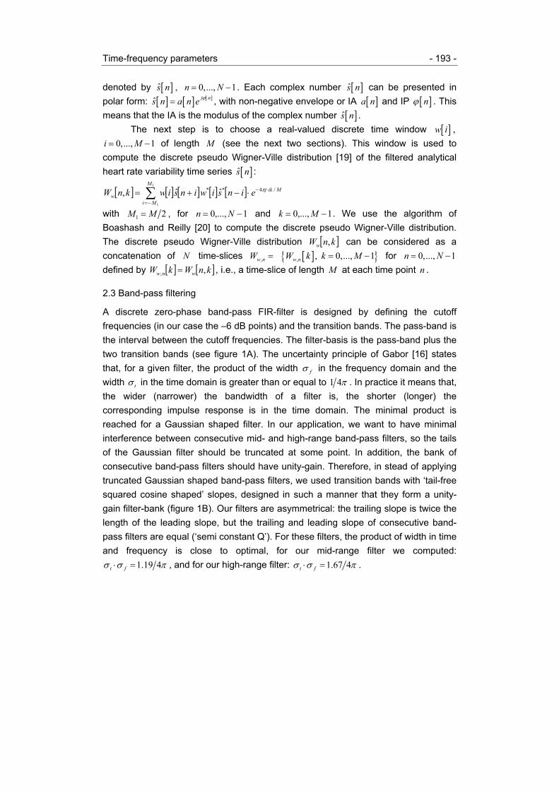
Time-frequency parameters - 193 -
denoted by [ ]s n , 0,..., 1n N= − . Each complex number [ ]s n can be presented inpolar form: [ ] [ ] [ ]ˆ j ns n a n e ϕ= , with non-negative envelope or IA [ ]a n and IP [ ]nϕ . Thismeans that the IA is the modulus of the complex number [ ]s n .
The next step is to choose a real-valued discrete time window [ ]w i ,0,..., 1i M= − of length M (see the next two sections). This window is used to
compute the discrete pseudo Wigner-Ville distribution [19] of the filtered analyticalheart rate variability time series [ ]s n :
[ ] [ ] [ ] [ ] [ ]∑−=
⋅−⋅−+=1
1
/4** ˆˆ,M
Mi
Mikjw einsiwinsiwknW π
with 1 2M M= , for 1,...,0 −= Nn and 1,...,0 −= Mk . We use the algorithm ofBoashash and Reilly [20] to compute the discrete pseudo Wigner-Ville distribution.The discrete pseudo Wigner-Ville distribution [ ]knWw , can be considered as aconcatenation of N time-slices ,w nW = [ ]{ }, , 0,..., 1w nW k k M= − for 0,..., 1n N= −defined by [ ] [ ]knWkW wnw ,, = , i.e., a time-slice of length M at each time point n .
2.3 Band-pass filtering
A discrete zero-phase band-pass FIR-filter is designed by defining the cutofffrequencies (in our case the –6 dB points) and the transition bands. The pass-band isthe interval between the cutoff frequencies. The filter-basis is the pass-band plus thetwo transition bands (see figure 1A). The uncertainty principle of Gabor [16] statesthat, for a given filter, the product of the width fσ in the frequency domain and thewidth tσ in the time domain is greater than or equal to 1 4π . In practice it means that,the wider (narrower) the bandwidth of a filter is, the shorter (longer) thecorresponding impulse response is in the time domain. The minimal product isreached for a Gaussian shaped filter. In our application, we want to have minimalinterference between consecutive mid- and high-range band-pass filters, so the tailsof the Gaussian filter should be truncated at some point. In addition, the bank ofconsecutive band-pass filters should have unity-gain. Therefore, in stead of applyingtruncated Gaussian shaped band-pass filters, we used transition bands with ‘tail-freesquared cosine shaped’ slopes, designed in such a manner that they form a unity-gain filter-bank (figure 1B). Our filters are asymmetrical: the trailing slope is twice thelength of the leading slope, but the trailing and leading slope of consecutive band-pass filters are equal (‘semi constant Q’). For these filters, the product of width in timeand frequency is close to optimal, for our mid-range filter we computed:
1.19 4t fσ σ π⋅ = , and for our high-range filter: 1.67 4t fσ σ π⋅ = .

- 194 - Chapter 9
The center frequency 0f is the midpoint of the filter-basis. Suppose wetranslate the center frequency to the zero frequency, then the filter-basis liessymmetrical around the zero frequency. Suppose the width of the filter-basis is B Hz.Then the new Nyquist frequency will be 1
2nf B= (figure 1C). Therefore, afterdemodulation of the signal with frequency 0f , it is sufficient to sample the filtered
1bf 2cf0f 2tf1cf 1tf 2bf
1.0
0.5
( )H f
2n sF F=
A
Figure1A. The design of a band-pass FIR-filter. The pass-band is the frequencyinterval [ ]1 2,c cf f , defined by the two cutoff frequencies, in our case –6 dB points,
1cf and 2cf . The filter-basis is the interval [ ]1 2,b bf f . The two transition bands[ ]1 1,b tf f and [ ]2 2,t bf f , are ‘squared cosine shaped’ slopes. The trailing slope ismade twice as long as of the leading slope. The center frequency 0f is themidpoint of the basis: ( )0 1 2 / 2b bf f f= + . The signal to be filtered is analytical,therefore there is no pass-band at the negative frequencies.
LOW MID HIGH 2sF
1.0
0.5
( )H f B
Figure 1B. The set of consecutive band-pass filters for the low-, mid-, and high-frequency components constitutes a unity-gain filter-bank. Trailing and leadingslopes of consecutive band-pass filter are equal.

Time-frequency parameters - 195 -
signal with sample rate B Hz. This means that, in the case of an ideal rectangularband-pass filter, the application of the translated low-pass filter in combination withcomplex demodulation will result in an over-sampled signal and the ‘over-samplingratio’ or ‘decimation factor’ DFn is DF sn F B= . In fact, we could decimate or down-sample the time series with a factor DFn and still retain the same information. In thisdown-sampled situation, the adjacent points in time are uncorrelated. In our case wedo not have ideal rectangular band-pass filters, but band-pass filters with squaredcosine shaped transition bands. This means that adjacent points are not trulyindependent.
The decimation factor DFn depends on the sample frequency sF and the widthof the filter-basis. The decimation factor DFn of our mid-range filter is 31. Todetermine the maximal discrete resolution t∆ in time, the Nyquist frequency of thedemodulated band-pass filter was determined to be
2sn
DF
Ffn
= =231
= 0.0645 Hz,
to allow for perfect signal integrity, whilst minimizing dependency between adjacentpoints in time. This leads to an optimal time resolution of 1 2 7.75nt f∆ = = sec (= 31samples). This means that computations over a shorter time interval yield adjacentlydependent results. Or, down-sampling with a factor smaller than 31 yieldsinterpolation. Computations over a longer time interval yield averaged results
1.0
2b nf f′ =1bf ′
( )H f
0.5
1cf ′ 2cf ′2tf ′1tf ′
C
Figure 1C. The filter-basis of the band-pass filter of figure 1A is translated over arange 0f towards the origin, 1 1 0b bf f f′ = − , 2 2 0b bf f f′ = − , etc. This basis of this filterlies symmetrical around the zero frequency. After demodulation of the signal withfrequency 0f , it is sufficient to sample the filtered signal with sample rate 22 bf ′⋅ .

- 196 - Chapter 9
(‘smearing’). Or, down-sampling with a factor larger than 31 yields aliasing.Examining the impulse response of the demodulated mid-range band-pass filter, wefound that there is a minimal dependency in the down-sampled demodulated timeseries over 3 data points (see chapter 7).
We now choose the window length M of the time window of the discretepseudo Wigner-Ville distribution to be DF 31n = points, in the case of the mid-rangeband-pass filter. This means that consecutive Wigner-Ville time-slices are computedover 7.75t∆ = sec. A shorter window leads to adjacently dependent time-slices, alonger window results in smearing. But in the case of the ideal length of 31 points, theadjacent time-slices are not truly independent, they show a minimal dependency over3 slices (see chapter 7).
In the case of our high-range band-pass filter we found that the decimationfactor DFn is 9 and the Nyquist frequency is nf = 2 9 = 0.2222 Hz. The optimal timeresolution is 2.25t∆ = sec (= 9 samples). We now choose the window length M ofthe discrete pseudo Wigner-Ville distribution to be DF 9n = points, and in this casethere is a minimal dependency between adjacent time-slices of 5 slices.
In conclusion, for the remainder of this article, ‘instantaneous’ is referred to asconsecutive points in time only showing a minimal dependency in time. For our mid-range filter, consecutive points are spaced over 7.75t∆ = sec with a dependency of 3points. For our high-range filter, consecutive points are spaced over 2.25t∆ = secwith a dependency of 5 points.
2.4 Implementation, part 2
The length M of the time window of the discrete pseudo Wigner-Ville distribution ischosen to be DFn , the decimation factor belonging to the mid- or high-range band-pass filter. For each time index n , we take the time-slice ,w nW of the discrete pseudoWigner-Ville distribution [ ],wW n k . This is a real data series in the frequency domain.It can be considered as an ‘instantaneous spectrum’, as mentioned above, but it isnot a true density, because it may contain negative values. Therefore, we determinethe squared envelope of each time-slice by computing the discrete analytical dataseries:
[ ],ˆw nW k = [ ],w nW k + [ ],w njHW k
and its squared modulus. We now compute the inverse discrete Fourier transform ofthe squared modulus in the index k :
[ ] [ ]21
ˆˆ ,ˆ,ssw k l w nR n l F W k−
→=

Time-frequency parameters - 197 -
for 1,...,0 −= Ml . We call the resultant [ ]lnR wss ,ˆˆ the discrete pseudo autocorrelationfunction (DPACF).
The computation of the discrete estimator [ ]nfw of the IF and the squaredestimator [ ]nBw
2 of the IB are now straightforward using the expressions:
[ ] [ ][ ]
⋅=
1,Re1,Imarctan
22/
ˆˆ
ˆˆ
nRnRFnf
wss
wsssw π
(5)
and
[ ] [ ][ ]0,1,
1ˆˆ
ˆˆ2
nRnR
nBwss
wssw −= (6)
corresponding with equations (3) and (4). These estimates are instantaneousconform the former section. As mentioned in the first Methods-section ‘Prerequisites’,phase unwrapping is not necessary in the computation of equation (5) and zerodivision in equation (6) cannot occur in case of non-zero signals.
The procedure of computing the envelope of the time-slice ,w nW can be seenas a smearing function in the frequency domain, i.e., convolution with an averagingfilter. It follows that in the τ -domain the inverse Fourier transform is weighted, i.e.,the DPACF is multiplied with a weighting function. But this means that [ ]nBw
2 is abiased squared estimator of the squared IB. The index [ ]nBw
2 , however, is useful asan indicator of irregularities or interference due to other signal components, as will bedemonstrated in the next sections. Therefore, this index is called the instantaneousbandwidth coefficient (IBC). The IBC [ ]nBw
2 is a qualitative index and is chosen insuch a way that it will always have a value between 0 and 1 (note the absence of thefactor 21 π in equation (6), e.g., equation (4)). Value 0 means that there is noamplitude modulation, so the signal is purely frequency modulated (see the Methods-section ‘Prerequisites’); value 1 means that the signal is a noise signal. The estimator
[ ]nfw is useful to calculate the IF and is not biased because both real and imaginarypart of [ ]1,ˆˆ nR wss have been multiplied by the same real factor of the weighting function.
2.5 The behavior of the IF and the IBC
In this section we describe the behavior of the IF and the IBC: 1) when the signal islocally, i.e., for a short period in time, not monocomponent, or, 2) due to the presenceof noise or random phase fluctuations in the original signal.1) A signal is locally multicomponent [12,13,19,23] in the frequency band of interestif there is locally more than one spectral concentration present in the time-varying‘instantaneous spectrum’. For instance, a signal may locally become multicomponentif harmonic or sub-harmonic components arise due to non-sinusoidal shape ofwaveforms. For multicomponent signals, the IF has no meaning [13]. The effect is

- 198 - Chapter 9
that phase shifts at low amplitudes cause discontinuities in the IF and the IBC. Forinstance, suppose ( )ts consists of two sinusoids with different frequencies 2 1f f>[33]:
( ) ( ) ( )( )d1 2 2 sign cos 2 f2 2ˆ 2 cos 2 hjf t j tjf t jf tds t e e f t e π π ππ π π + ⋅= + =
in which ( )2 1 2df f f= − and ( )1 2 2hf f f= + . The signal ( )ts is a complex analyticalsignal and the IA is ( ) ( )2 cos 2 da t f tπ= . The double sinusoid shows phase shifts of2π± at each time the cosine function ( )cos 2 df tπ of the IA changes sign. Phase shifts
cause discontinuities in the IF, because the IF is the derivative (1) of the phase. Itfollows from equation (2) that the IBC is approximated by ( ) ( )2 2 2 2tan 2i d dB t f f tπ π= .Therefore, there are high peaks in the IBC at times where the cosine function
( )cos 2 df tπ changes sign.2) Random phase fluctuations may have various origins. It may be quantizationnoise due to R-wave detection errors. It may also be physiological noise originatingfrom stochastic components of the underlying physiological system. Under pure noiseconditions, neighbouring samples in time are uncorrelated. If noise is present in thesignal, this may result in ‘sudden’ phase shifts. ‘Sudden’ phase shifts, in turn, mayresult in discontinuities in the IF, as explained above. Also, the autocorrelationfunction at 1τ = of a noisy signal is zero in expectation, but varies randomly.Therefore, the IBC (see equations (4) and (6)) of a noisy signal varies randomly andwill show outlier peaks. By nature, the IBC is peaked at all phase shifts.
An illustration of the peaks in the IBC is provided in figure 2B. The middle andlower graph present the IF and the IBC derived from a mid-frequency range heartrate variability time series. High peaks in the IBC coincide with discontinuities in theIF. The deflections in the IF and the IBC are due to aliasing because the samplefrequency is too low to catch the slope of the peaks.
2.6 How to use the IBC?
The IBC may be used to locate irregularities or discontinuities in the IF due to(sudden) phase shifts. The IBC is an index between 0 and 1. A suitable threshold canbe chosen such that IBC-values above this threshold indicate discontinuities in the IF;corresponding segments in time of the IF can be excluded from further analysis andthe time-frequency parameters can now be computed.
However, the IF of a noisy or irregular signal may sometimes behave ‘regular’.In that case, the IBC cannot discriminate between a ‘regular’ IF of an irregular timesegment and an oscillatory time segment of a signal. In general, we assume the IA ofan irregular time segment of a signal to be low-valued in our frequency bands of

Time-frequency parameters - 199 -
interest. It is therefore that an alternative index is defined that involves both the IAand the IBC to discriminate between irregular and oscillatory time segments and,simultaneously, to exclude discontinuities in the IF. This signal is called the‘amplitude-corrected instantaneous bandwidth coefficient (ACIBC)’ and is defined by:
( ) ( )( ) ( )IA
ACIBCIA IBC
tt
t t=
+This is an index between 1 and 0. If the IA is high-valued, the ACIBC is high (close to1). If the signal is irregular, i.e., has a low-valued IA, the ACIBC is low-valued (closeto 0). Upward peaks in the IBC correspond to downward peaks (close to 0) in theACIBC. Therefore, low ACIBC-values mean that the signal is locally irregular anddownward peaks indicate discontinuities in the IF. A threshold can be chosen suchthat ACIBC-values under this threshold indicate irregularities and downward peaksunder this threshold indicate discontinuities in the IF. Figure 2B presents an ACIBCtime series (upper graph) associated with the IBC (lower graph) and the IF (middlegraph) derived from a heart rate variability time series in the mid-frequency band. Theoriginal heart rate variability time series, the mid-frequency heart rate variability, andthe IA are presented in figure 2A.
In this manner, the IBC and the ACIBC are used to exclude or reject certainshort periods of time in the signal under analysis. The rejected periods in time definecorresponding samples of the IF and the IA, which are to be removed from furtheranalysis. The IBC is used to remove discontinuities from the IF, whereas the ACIBCis used for the simultaneous removal of discontinuities from the IF and irregular partsfrom the IA. Threshold levels determine the rejected periods. A threshold level of, forinstance, 0.25 or 25% means that samples with corresponding IBC-values higherthan 0.25 are rejected or, when using the ACIBC, that samples with correspondingACIBC-values lower than 0.75 are rejected. In both cases, a lower threshold levelmeans that, in general, more samples will be rejected and will result in larger rejectedperiods. When a number ( 1≥ ) of adjacent samples is detected for rejection, then ateach side this group is supplemented with 2DFn adjacent samples. Together theyform the rejected period. Thus a rejected period is at least DFn samples wide. Thiswidening is done to also remove the slopes of a discontinuity in the IF. In figure 3A,Bthe rejected periods are shown as windows spanning the discontinuities in the IFincluding the slopes of the discontinuities. The complementary accepted samples arealso grouped in accepted periods (of length 1≥ samples).
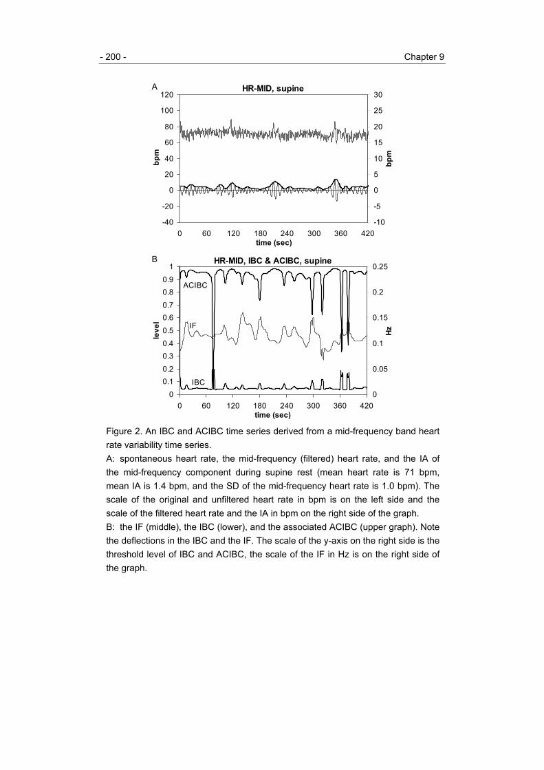
- 200 - Chapter 9
HR-MID, supine
-40
-20
0
20
40
60
80
100
120
0 60 120 180 240 300 360 420time (sec)
bpm
-10
-5
0
5
10
15
20
25
30
bpm
A
HR-MID, IBC & ACIBC, supine
00.10.20.30.40.50.60.70.80.9
1
0 60 120 180 240 300 360 420time (sec)
leve
l
0
0.05
0.1
0.15
0.2
0.25
Hz
ACIBC
IBC
B
IF
Figure 2. An IBC and ACIBC time series derived from a mid-frequency band heartrate variability time series.A: spontaneous heart rate, the mid-frequency (filtered) heart rate, and the IA ofthe mid-frequency component during supine rest (mean heart rate is 71 bpm,mean IA is 1.4 bpm, and the SD of the mid-frequency heart rate is 1.0 bpm). Thescale of the original and unfiltered heart rate in bpm is on the left side and thescale of the filtered heart rate and the IA in bpm on the right side of the graph.B: the IF (middle), the IBC (lower), and the associated ACIBC (upper graph). Notethe deflections in the IBC and the IF. The scale of the y-axis on the right side is thethreshold level of IBC and ACIBC, the scale of the IF in Hz is on the right side ofthe graph.

Time-frequency parameters - 201 -
HR-HIGH, IF & IBC 30, supine
0
0.1
0.2
0.3
0.4
0.5
0 50 100 150 200time (sec)
Hz
0
0.05
0.1
0.15
0.2
0.25
0.3
0.35
leve
l
A
HR-HIGH, IF & IBC 25, supine
0
0.1
0.2
0.3
0.4
0.5
0 50 100 150 200time (sec)
Hz
0
0.05
0.1
0.15
0.2
0.25
0.3
0.35
leve
l
B
Figure 3. IBC threshold levels: the graphs A and B show the same IF of a high-frequency band heart rate variability time series and the effects of differentthreshold levels. The scale of the IF in Hz is on the left side and the threshold levelof the IBC is on the right side of the graph. The IBC is used to locatediscontinuities in the IF and the rejected periods are marked with windows.Rejected periods in graph A are determined by means of an IBC threshold level of30%. The rejected fraction is 3.4%. The IBC threshold level of graph B is 25%,yielding a rejected fraction of 8.1%.

- 202 - Chapter 9
2.7 Definition of the time-frequency parameters
This section defines several time-frequency parameters for each IA and IF timeseries of the mid- and high-frequency band. These parameters take into account theperiods that are accepted or rejected by means of the IBC or the ACIBC. Assumethat the time segment under analysis consists of N samples, the total time of thetime segment is sT N t= ⋅ , because the sample interval is st . The IBC and the ACIBCare used to exclude or reject certain parts or periods within the time segment. Thisleads to rejecting a total number rejN of samples in the rejected periods. Then thetotal duration of the rejected periods is rej rej sT N t= ⋅ . A complementary number ofsamples acc rejN N N= − is accepted. The duration of the accepted periods is
acc acc s rejT N t T T= ⋅ = − .
2.7.1 Time parameters• The Rejected Fraction is the fraction of the time segment that is rejected:
( )RF 100 %rejT T= × .
• The Accepted Fraction is the complementary fraction of the time segment that isaccepted:
( )AF 100 %accT T= × .
2.7.2 IF and IA parameters• The Mean Instantaneous Amplitude is computed with:
( ) [ ]IA 1 IAacc
accn N
N n∈
= ∑after removing the rejected samples from the IF and/or the IA time series: accn N∈means that only accepted samples are used.• The Mean Square Instantaneous Amplitude is computed in the same way:
( ) [ ]22IA 1 IAacc
accn N
N n∈
= ∑The mean square instantaneous amplitude is a measure of the spectral power of thesignal in the frequency band of interest.• The Mean Instantaneous Frequency in the time segment is computed with:
( ) [ ]IF 1 IFacc
accn N
N n∈
= ∑• The Mean Frequency is the weighed mean IF using the square IA as weight. It iscomputed with:
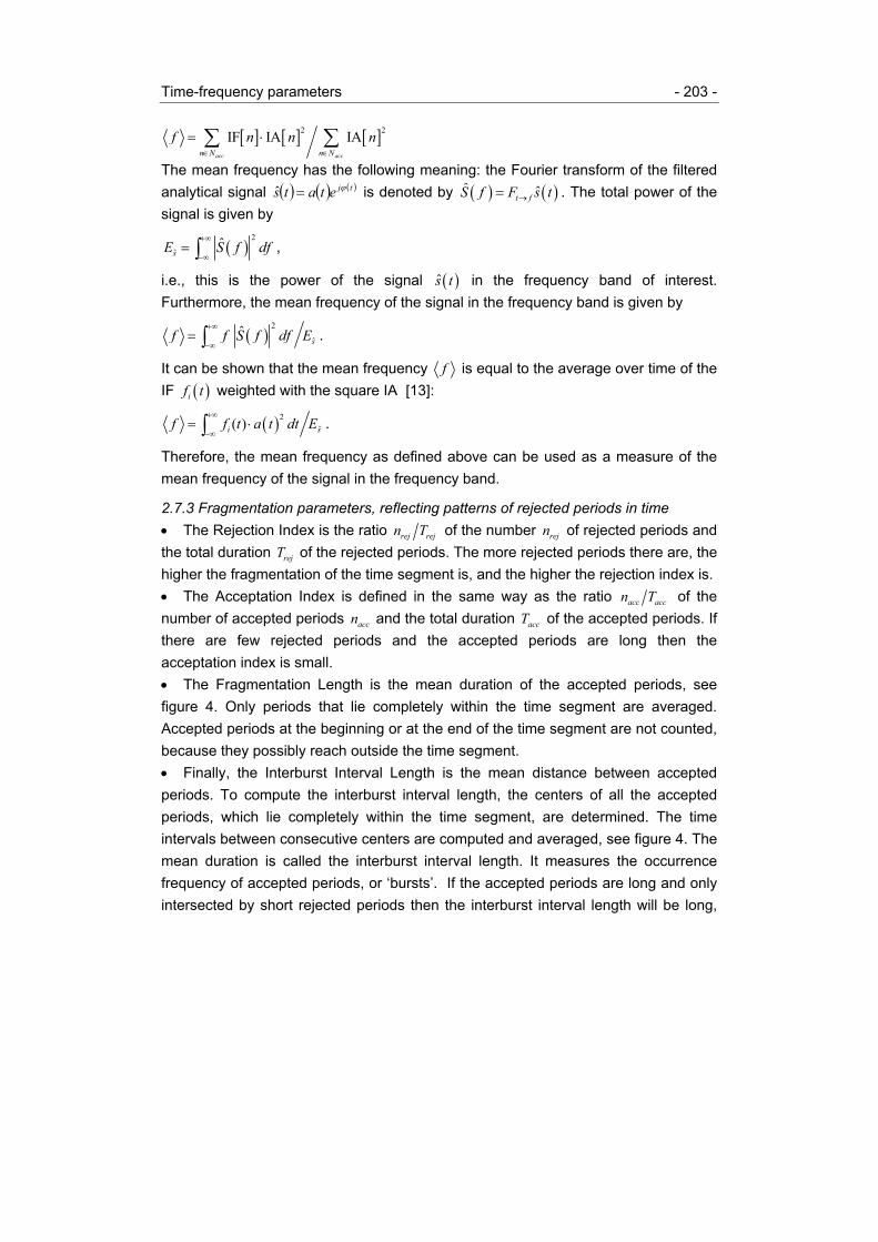
Time-frequency parameters - 203 -
[ ] [ ] [ ]2 2IF IA IAacc accn N n N
f n n n∈ ∈
= ⋅∑ ∑The mean frequency has the following meaning: the Fourier transform of the filteredanalytical signal ( ) ( ) ( )tjetats ϕ=ˆ is denoted by ( ) ( )ˆ ˆt fS f F s t→= . The total power of thesignal is given by
( )2
ˆˆ
sE S f df+∞
−∞= ∫ ,
i.e., this is the power of the signal ( )s t in the frequency band of interest.Furthermore, the mean frequency of the signal in the frequency band is given by
( )2
ˆˆ
sf f S f df E+∞
−∞= ∫ .
It can be shown that the mean frequency f is equal to the average over time of theIF ( )if t weighted with the square IA [13]:
( )2 ˆ( )i sf f t a t dt E+∞
−∞= ⋅∫ .
Therefore, the mean frequency as defined above can be used as a measure of themean frequency of the signal in the frequency band.
2.7.3 Fragmentation parameters, reflecting patterns of rejected periods in time• The Rejection Index is the ratio rej rejn T of the number rejn of rejected periods andthe total duration rejT of the rejected periods. The more rejected periods there are, thehigher the fragmentation of the time segment is, and the higher the rejection index is.• The Acceptation Index is defined in the same way as the ratio acc accn T of thenumber of accepted periods accn and the total duration accT of the accepted periods. Ifthere are few rejected periods and the accepted periods are long then theacceptation index is small.• The Fragmentation Length is the mean duration of the accepted periods, seefigure 4. Only periods that lie completely within the time segment are averaged.Accepted periods at the beginning or at the end of the time segment are not counted,because they possibly reach outside the time segment.• Finally, the Interburst Interval Length is the mean distance between acceptedperiods. To compute the interburst interval length, the centers of all the acceptedperiods, which lie completely within the time segment, are determined. The timeintervals between consecutive centers are computed and averaged, see figure 4. Themean duration is called the interburst interval length. It measures the occurrencefrequency of accepted periods, or ‘bursts’. If the accepted periods are long and onlyintersected by short rejected periods then the interburst interval length will be long,

- 204 - Chapter 9
i.e., the occurrence frequency of accepted periods is low. But, the more rejectedperiods there are, the shorter the interburst interval length will be.
3 Application
3.1 Quantification of duration and number of irregular periods for obtaining time-frequency parameters
To quantify (and correct the IA and IF time series of the mid- and high-frequencyband for) the duration and number of (rejected) periods of irregularities, the followingapproach was used. Based on the instantaneous bandwidth coefficient (IBC) and theamplitude-corrected instantaneous bandwidth coefficient (ACIBC), several thresholdlevels were defined and evaluated for their effectiveness in indicating and removingthe sequential periods of irregularities from IA and IF time series. These thresholdlevels were chosen based on visual inspection by two researchers of the originalheart rate variability time series and the corresponding IA and IF time series of 10min periods of supine rest and orthostatic challenge of 10 healthy subjects and 10patients with autonomic dysfunction showing abnormal mid- and high-frequencyfluctuations (cardiac transplant recipients; autonomic failure). Figure 3A,B illustratesfor the high-frequency band the effect of different and decreasing threshold levels(30% and 25%) of the IBC on the detection of irregularities in the IF time series:choosing the wrong level may lead to either underestimation or overestimation of thepresence of irregularities and thereby influence reliable computation of the time-frequency parameters. As a first approach, our aim was to remove only those periodsfrom the time series that both researchers unequivocally defined as irregularities.
ii ii ii ii
r r r ra a a
Figure 4. The definition of the fragmentation length and the interburst intervallength. The rejected periods of a time segment are marked with r. The meanduration of the accepted periods (a) is the fragmentation length. Interburstintervals are the time intervals between the centers of two consecutive acceptedperiods a, they are marked with ii. Each interburst interval spans a rejected periodr. The mean duration of the interburst intervals is the interburst interval length.

Time-frequency parameters - 205 -
Systematic inspection of our data revealed that for an accurate correction forirregularities of the mid-frequency fluctuations, the ACIBC with a threshold level of 25appeared suitable for most time series, wheres as for the high-frequency band anIBC threshold level of 30 was adequate to quantify unequivocal irregular periods.
3.2 Subjects, procedures, and measurements
Data of 39 healthy volunteers (13 females, 26 males; mean age: 36.6 years, SD:15.3, range: 19 – 68) were obtained from several experiments in which cardio-vascular recordings were made during periods of supine rest and orthostaticchallenge [e.g., 9,34].
The recording sessions for the cardiovascular parameters were alwaysperformed in the morning. After a stabilization period (of at least 15 min), recordingswere obtained during: supine rest (10 min) and orthostatic challenge (active standingor 60 degrees head-up tilt by means of the tilt-table; 10 min). Spontaneousfluctuations in breathing, heart rate, and blood pressure were recorded: the subjectswere asked to relax and to breath regularly, not to speak, to move as little aspossible, and to stay awake.
ECG, BP (Finapress) and respiration were recorded continuously andanalysed according to methods described previously [9,34]. Only time-frequencyanalyses of the spontaneous variations in heart rate during supine rest andorthostatic challenge will be presented in this paper.
Statistical AnalysesThe complete 10-min heart rate variability time series of supine rest was used for thecomputation of the time-frequency parameters. For the standing period, the first 2minutes after standing were discarded because, as a first approach, we wanted todescribe the time-frequency parameters during a steady state situation (last 8 minperiod of standing). For the mid- and high-frequency band separately, mean (SD)values of the time-frequency parameters are presented per condition (supine,standing). Differences in mean heart rate and the time-frequency parameters of themid- and high-frequency band between supine rest and standing were evaluated bymeans of Student’s t-tests for pairwise comparisons. If the parameter was notnormally distributed, a non-parametrical test was applied (Wilcoxon test). Statisticalanalyses were performed using the SPSS for Windows Release 9.0. A p-value of<0.05 was used to indicate a significant effect.

- 206 - Chapter 9
4 Results
Mean heart rate showed a significant increase from supine rest to standing (onaverage, mean % change: +20%; table 1; figure 5A,B).
Time-frequency parameters of the mid-frequency bandFigure 5A,B and 6A,B show typical examples of spontaneous changes in heart rate,IA, and IF of the mid-frequency band during supine rest and orthostatic challenge ofan individual subject. In comparison with supine rest, during standing the IA appearsincreased (figure 5), whereas the IF appears decreased (figure 6). Furthermore, lessdata periods are discarded as irregular periods, resulting in longer fragmentationlengths (figure 6). Figure 5 also illustrates an increase in variability of the mid-frequency band (filtered) heart rate from supine rest to standing. On group level, fromsupine rest to standing, the accepted fraction (+10%), the mean IA (+40%), the meansquare IA (+124%), the rejection index (+13%), and the fragmentation length (+23%)increased significantly, whereas the rejected fraction (-32%), the mean IF (-9%), andthe acceptation index (-26%) showed a significant decrease (table 1).
Time-frequency parameters of the high-frequency bandSpontaneous changes in heart rate, the IA, and the IF of the high-frequency bandduring supine rest and standing of an individual subject are presented in figures 7and 8: from supine rest to standing, the variability of the high-frequency heart rate aswell as the IA of the high-frequency component are decreased (figure 7); the IFappears decreased and there are more rejected periods, resulting in shorterfragmentation lengths (figure 8). On group level, from supine rest to standing, themean IA (-22%), the mean square IA (-135%), the mean IF (-4%), the fragmentationlength (-45%), and the interburst interval length (-40%) decreased significantly (table1). We observed no significant changes from supine rest to standing in the acceptedor rejected fractions.
5 Discussion
5.1 Time-frequency parameters during supine rest and orthostatic challenge
Supine restOn average, 24% of the time periods of the mid- and the high-frequency band weredefined as irregularities/discontinuities, indicating that for 76% of the time periods themonocomponent assumption of our method appeared valid. The mean IF of the mid-frequency band during supine rest was 0.11 Hz (mean cycle length: 9.1 sec),

Time-frequency parameters - 207 -
Table 1: Mean (SD) of heart rate and time-frequency parameters of the mid- andhigh-frequency component during supine rest and standing.
Supine Standing t-test
N=39 mean (SD) mean (SD) t; p values
Heart Rate (bpm) 67.9 (8.1) 81.8 (10.3) -8.6; <.001
Mid-frequency band
Accepted Fraction (%) 76.5 (10.5) 83.9 (12.2) -4.1; <.001
Rejected Fraction (%) 23.6 (10.5) 16.1 (12.2) 4.1; <.001
Mean IA (bpm) 1.15 (0.5) 1.61 (0.9) -3.7; =.001
Mean Square IA (ln) 0.38 (0.8) 0.85 (1.2) -3.4; =.002
Mean IF (Hz) 0.11 (0.007) 0.10 (0.008) 4.2; <.001
Mean Frequency (Hz) 0.11 (0.005) 0.10 (0.006) 5.5; <.001
Acceptation Index*100 2.7 (1.4) 2.0 (1.5) 2.8; =.008
Rejection Index*100 8.0 (1.0) 9.0 (1.6) -4.2; <.001
Fragmentation Length (sec) 44.6 (23.8) 54.8 (32.2) -2.0; =.050
Interburst Interval Length (sec) 57.6 (23.9) 62.7 (26.6) -1.4; NS
High-frequency band
Accepted Fraction (%) 76.4 (14.6) 73.1 (11.8) 1.6; NS
Rejected Fraction (%) 23.6 (14.6) 26.9 (11.7) -1.6; NS
Mean IA (bpm) 1.15 (0.6) 0.90 (0.4) 3.2; =.003
Mean Square IA (ln) 0.31 (0.9) -0.11(0.9) 3.2; =.002
Mean IF (Hz) 0.25 (0.028) 0.24 (0.028) 2.6; =.013
Mean Frequency (Hz) 0.25 (0.025) 0.24 (0.025) 3.2; =.003
Acceptation Index*100 10.3 (7.6) 11.7 (6.7) -1.1; NS
Rejection Index*100 30.1 (2.6) 29.5 (2.4) 1.2; NS
Fragmentation Length (sec) 23.3 (30.9) 12.9 (11.4) 2.3; =.030
Interburst Interval Length (sec) 28.2 (36.8) 16.8 (12.9) 2.0; =0.50
NS: non-significant

- 208 - Chapter 9
HR-MID supine
-40
-20
0
20
40
60
80
100
120
0 120 240 360 480time (sec)
bpm
-10
-5
0
5
10
15
20
25
30
bpm
A
HR-MID standing
-40
-20
0
20
40
60
80
100
120
0 120 240 360 480time (sec)
bpm
-10
-5
0
5
10
15
20
25
30
bpm
B
Figure 5. Spontaneous changes in heart rate, mid-frequency band (filtered) heartrate and the IA of the mid-frequency component during supine rest (A) andorthostatic challenge (B). Mean heart rate increases from 55 pm during supine restto 88 bpm during standing. The SD of the mid-frequency band heart rate increasesfrom 0.9 bpm to 3.0 bpm. Mean IA of the mid-frequency component increasesfrom 1.0 bpm to 3.9 bpm. The scale of the original and unfiltered heart rate in bpmis on the left side and the scale of the filtered heart rate and the IA in bpm on theright side of the graph.
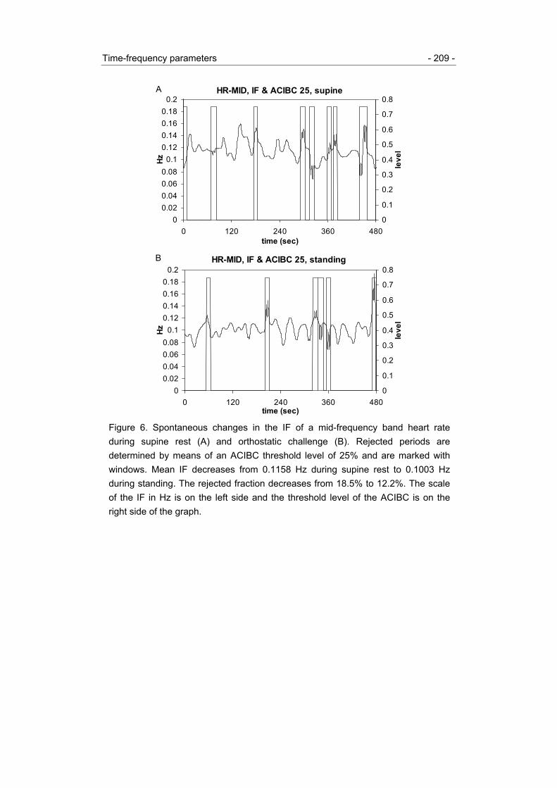
Time-frequency parameters - 209 -
HR-MID, IF & ACIBC 25, supine
00.020.040.060.08
0.10.120.140.160.18
0.2
0 120 240 360 480time (sec)
Hz
0
0.1
0.2
0.3
0.4
0.5
0.6
0.7
0.8
leve
l
A
HR-MID, IF & ACIBC 25, standing
00.020.040.060.08
0.10.120.140.160.18
0.2
0 120 240 360 480time (sec)
Hz
0
0.1
0.2
0.3
0.4
0.5
0.6
0.7
0.8
leve
l
B
Figure 6. Spontaneous changes in the IF of a mid-frequency band heart rateduring supine rest (A) and orthostatic challenge (B). Rejected periods aredetermined by means of an ACIBC threshold level of 25% and are marked withwindows. Mean IF decreases from 0.1158 Hz during supine rest to 0.1003 Hzduring standing. The rejected fraction decreases from 18.5% to 12.2%. The scaleof the IF in Hz is on the left side and the threshold level of the ACIBC is on theright side of the graph.

- 210 - Chapter 9
HR-HIGH supine
-20
0
20
40
60
80
100
120
0 60 120 180 240 300time (sec)
bpm
-5
0
5
10
15
20
25
30
bpm
A
HR-HIGH standing
-20
0
20
40
60
80
100
120
0 60 120 180 240 300time (sec)
bpm
-5
0
5
10
15
20
25
30
bpm
B
Figure 7. Spontaneous changes in heart rate, high-frequency band (filtered) heartrate and the IA of the high-frequency component during supine rest (A) andorthostatic challenge (B). Mean heart rate increases from 69 bpm during supinerest to 99 bpm during standing. The SD of the high-frequency band heart ratedecreases from 1.2 bpm to 0.9 bpm. Mean IA of the high-frequency componentdecreases from 1.7 bpm during supine rest to 1.1 bpm during standing. Thescale of the original and unfiltered heart rate in bpm is on the left side and thescale of the filtered heart rate and the IA in bpm on the right side of the graph.

Time-frequency parameters - 211 -
HR-HIGH, IF & IBC 30, supine
0
0.1
0.2
0.3
0.4
0.5
0 60 120 180 240 300time (sec)
Hz
0
0.05
0.1
0.15
0.2
0.25
0.3
0.35
leve
l
A
HR-HIGH, IF & IBC 30, standing
0
0.1
0.2
0.3
0.4
0.5
0 60 120 180 240 300time (sec)
Hz
0
0.05
0.1
0.15
0.2
0.25
0.3
0.35
leve
l
B
Figure 8. Spontaneous changes in the IF of a high-frequency band heart rateduring supine rest (A) and orthostatic challenge (B), derived of the same dataset, i.e. the high-frequency heart rate, of figure 7. Rejected periods aredetermined by means of an IBC threshold level of 30% and are marked withwindows. Mean IF decreases from 0.2873 Hz during supine rest to 0.2146 Hzduring standing. The rejected fraction increases from 2.1% to 13.6%. The scaleof the IF in Hz is on the left side and the threshold level of the ACIBC is on theright side of the graph.

- 212 - Chapter 9
the mean IF of the high-frequency band was 0.25 Hz (mean cycle length: 4 sec).Under the present conditions, we observed a fragmentation length of 45 sec and aninterburst interval length of 58 sec for the mid-frequency band and a fragmentationlength of 23 sec and an interburst interval length of 28 sec for the high-frequencyband. The large standard deviations of these parameters reflect the large inter-individual variability in fragmentation and interburst interval length.
Orthostatic challengeWhen changing from supine to standing posture, initial changes in heart rate occurthat are different from the steady state variations after prolonged standing (afterabout 2 min) [35]. Although it is interesting to describe the time-frequency variationsof the initial heart rate changes [e.g., 36], in this study our focus was on the time-frequency variations in heart rate during steady state (last 8 min of the 10 minstanding period) to explore the relevance of the characteristics of the oscillatory andirregular periods in the heart rate series and compare it with a steady state situationduring supine rest.
Mid-frequency bandBased on spectral analyses, mid-frequency band power of heart rate has beenshown to increase [e.g., 10,37]. Overall, our results are in line with these studies,although our time-frequency parameters revealed an additional effect of standing onIA and IF: whereas IA increased significantly, IF showed a minor, but significant,decrease. Regarding the characteristics of the oscillatory and irregular periods, therejected fraction decreased during standing (-32%), an effect that was accompaniedby an increase in fragmentation length but no significant change in interburst intervallength. On average, about 84% of the mid-frequency signal could be considered asbeing monocomponent. Apparently, during standing there is an increase inappearance, strength and length of a mid-frequency oscillation as reflected in anincreased amplitude, cycle length, and less interference of irregularities.
High-frequency bandBased on spectral analyses, high-frequency power of heart rate has repeatedly beenshown to decrease as a result of vagal inhibition [e.g., 10,37,38]. Our time-frequencyparameters also revealed a significant decrease of IA, an effect that wasaccompanied by a small, but significant, decrease of IF (mean cycle length increasedfrom 4 to 4.2 sec, probably reflecting a somewhat slower breathing rate duringstanding). In contrast to the mid-frequency band, the rejected fraction showed nosignificant change from supine to standing, although significant decreases infragmentation length and interburst interval length were observed. It is presently

Time-frequency parameters - 213 -
unclear whether these effects are the result of a more variable or complex breathingpattern from supine to standing posture. Cross-analyses with time-frequencychanges in the respiratory signal itself are necessary to further clarify these findings.
5.2 Time-frequency parameters: future developments
As a first approach, the data of this study were quantified by means of selectedthreshold levels of the IBC and the ACIBC. Although these threshold levels werechosen on the basis of visual screening of a sample of heart rate time series ofhealthy subjects and patients with autonomic dysfunction by two researchers, we canpresently not conclude that the thresholds were optimal for every heart rate timeseries. Further studies are necessary to optimize the choice of thresholds. However,computations on the basis of the presently used threshold levels showed that it isinteresting to quantify time-varying characteristics of signal and irregularities. Thesignificant effect of the changing of posture on the amount of irregularities detected,as well as on the fragmentation length and the interburst interval length indicates thatthese parameters may have physiological relevance. Furthermore, it also suggeststhe presence of a periodic process in the occurrence of irregularities that can beinfluenced by external circumstances. However, since the occurrence of irregularitiesand interference can be the result of multiple processes (harmonic or sub-harmoniccomponents, quantization or physiological noise, see the Methods-section: ‘Thebehavior of the IF and the IBC’) and standard deviations in our group were ratherlarge, these processes need to be further elucidated by studying cardiovascularvariability of various patients groups (CHD, hypertension, autonomic failure,neurological and psychiatric disorders) under various conditions (physical strain,psychological stress, cardiovascular and psychoactive drugs).
Complementary to conventional sequential spectral analysis, which has a timeresolution of about 2-5 min, our time-frequency method provides instantaneousinformation of time-varying cardiovascular changes with a time resolution of about 8sec for the mid-frequency band and about 2.5 sec for the high-frequency band. Thishigh time resolution of the time-varying spectral description, provided by IA and IF,may contribute to a more detailed description of the time-varying dynamics ofcardiovascular signals. For instance, periods with phase shifts, i.e., discontinuities inthe IF, may be submitted to further analysis, such as cross-correlation betweendifferent frequency bands or different cardiovascular time series, to investigatepossible dependencies and harmonic relationships between frequency bands. Or,transient changes in cardiovascular variability may be investigated [e.g., 39].Considering the effect of breathing on heart rate variability, it appears essential in

- 214 - Chapter 9
future studies to include analyses of respiratory parameters and perform cross-correlational studies. The method presented in this paper can be directly applied toother cardiovascular signals (e.g., blood pressure) as well as to respiratory signals;computation of time-dependent changes in transfer functions between two signals issimilarly feasible and interesting to perform [7,40].
In summary, we have evaluated a new method to compute time-frequencyparameters from cardiovascular time series. Apart from calculating the IA and the IF,characteristics of the oscillatory and irregular periods can be quantified that may berelevant to further unravel the situational- and state-dependent dynamics ofhomeostatic cardiovascular control processes. As a first approach, the method wasapplied to describe changes in time-frequency parameters and in the characteristicsof the oscillatory and irregular periods from supine to standing posture, under steadystate conditions in healthy subjects. The parameters and characteristicsdiscriminated differentially between supine rest and orthostatic challenge.Furthermore, the method can be applied to other cardiovascular time series providedthey are monocomponent.
Acknowledgements
The authors like to thank prof. ir. K.H. Wesseling of the department TNO-BMI of theUniversity of Amsterdam for his kind help regarding the preparation of this paper.
References
[1] Akselrod S, Gordon D, Madwed JB, Snidman NC, Shannon DC, and Cohen RJ:Hemodynamic regulation: investigation by spectral analysis. Am J Physiol249:M867-M875, 1985.
[2] Kitney RI: Beat-by-beat interrelationships between heart rate, blood pressureand respiration. In: Beat-to-beat Investigation of Cardiovascular Function. R.I.Kitney and O. Rompelman, Eds. Oxford: Oxford University Press, pp 146-178,1985.
[3] Sayers BMcA: Analysis of heart rate variability. Ergonomics 16:17-32, 1973.[4] Sayers BMcA: Signal analysis of heart-rate variability In: The Study of Heart-
Rate Variability. R.I. Kitney and O. Rompelman, Eds. Oxford: Clarendon Press,pp 27-58, 1980.
[5] Kobayashi M and Musha T: 1/f Fluctuations of heartbeat period. IEEE TransBiomed Eng BME-29:456-457, 1982.

Time-frequency parameters - 215 -
[6] Baselli G, Cerutti S, Civardi S, Malliani A, and Pagani M: Cardiovascularvariability signals: towards the identification of a closed-loop model of the neuralcontrol mechanisms. IEEE Trans Biomed Eng BME-35:1033-1046, 1988.
[7] Saul JP, Berger RD, Albracht P, Stein SP, Chen MH, and Cohen RJ: Transferfunction analysis of the circulation: unique insights into cardiovascularregulation. Am J Physiol 261:H1231-H1245, 1991.
[8] Tulen JHM, Man in 't Veld AJ, van Roon AM, Moleman P, van Steenis HG,Blankestijn PJ, and Boomsma F: Spectral analysis of hemodynamics duringinfusions of epinephrine and norepinephrine in men. J Appl Physiol 76(5):1914-1921, 1994.
[9] Tulen JHM, Bruijn JA, de Man KJ, Pepplinkhuizen L, van den Meiracker AH,and Man in 't Veld AJ: Cardiovascular variability in major depressive disorderand effects of imipramine or mirtazapine (Org 3770). J Clin Psychopharmacol16(2):135-145, 1996.
[10] Tulen JHM, Boomsma F, and Man in 't Veld AJ: Cardiovascular control andplasma catecholemines during rest and mental stress: effects of posture.Clinical Science 96:567-576, 1999.
[11] Parati G, Castiglioni P, di Renzo M, Omboni S, Pedotti A, and Mancia G:Sequential spectral analysis of 24-hour blood pressure and pulse interval inhumans. Hypertension 16:414-421, 1990.
[12] Boashash B: Estimating and interpreting the instantaneous frequency of asignal – part 1: fundamentals. Proc IEEE 80(4):520-538, 1992.
[13] Cohen L: Time-Frequency Analysis. Englewood Cliffs, NJ: Prentice Hall, 1995.[14] van Steenis HG, Martens WLJ, and Tulen JHM: Quantification of the dynamic
behaviour over time of narrow-band components present in heart rate variabilityby means of the instantaneous amplitude and frequency. submitted a.
[15] van Steenis HG, Martens WLJ, and Tulen JHM: The instantaneous frequency ofcardiovascular time series: a comparison of methods. submitted b.
[16] Gabor D: Theory of communication. Proc IEE 93(III):429-457, 1946.[17] Ville J: Théorie et application de la notion de signal analytique. Cables et
Transmissions 2A(1):61-74, 1948.[18] Wigner E: On the quantum correction for thermodynamic equilibrium. Phys Rev,
40:749-759, 1932.[19] Boashash B: Time-frequency signal analysis. In: Advances in Spectrum
Analysis and Array Processing, Vol. 1. S. Haykin, Ed. Englewood Cliffs, NJ:Prentice Hall, pp 418-517, 1991.
- 216 - Chapter 9
[20] Boashash B and Reilly A: Algorithms for time-frequency signal analysis. In:Time Frequency Signal Analysis – Methods and Applications, chapter 7. B.Boashash, Ed. Longman Cheshire, 1992.
[21] Oppenheim AV, Schafer RW, and Buck JR: Discrete-Time Signal Processing,2nd edition. Englewood Cliffs, NJ: Prentice Hall, 1999.
[22] Rihaczek A: Signal energy distribution in time and frequency. IEEE Trans.Inform. Theory IT-14:369-374, 1968.
[23] Choi HI and Williams WJ: Improved time-frequency representation ofmulticomponent signals using exponential kernels. IEEE Trans Acoust Speech,Signal Processing ASSP-37:862-871, 1989.
[24] Cohen L and Lee C: Instantaneous bandwidth. In: Time Frequency SignalAnalysis – Methods and Applications, chapter 4. B. Boashash, Ed. LongmanCheshire, 1992.
[25] Bendat JS and Piersol AG: Random Data, Analysis and MeasurementsProcedures, 2nd edition. New York: John Wiley and Sons, Inc., 1986.
[26] Angelsen BAJ: Instantaneous frequency, mean frequency and variance of meanfrequency estimatores for ultrasonic blood velocity doppler signals. IEEE TransBiomed Eng BME-28:733-741, 1981.
[27] Martens WLJ: The fast time frequency transform (F.T.F.T.): a novel on-lineapproach to the instantaneous spectrum. 14th International Conference of theIEEE Engineering in Medicine and Biology Society, 1992, Paris.
[28] Martens WLJ: Segmentation of ‘rhythmic’ and ‘noisy’ components of sleep EEG,heart rate and respiratory signals based on instantaneous amplitude, frequency,bandwidth and phase. 1st joint BMES/EMBS conference 1999, Atlanta.
[29] Bayly EJ: Spectral analysis of pulse frequency modulation in the nervoussystem. IEEE Trans Biomed Eng BME-15:257-265, 1968.
[30] Hyndman BW and Mohn RK: A model of the cardiac pacemaker and its use indecoding the information content of cardiac intervals. Automedica 1:239-252,1975.
[31] Rompelman O: The assessment of fluctuations in heart rate. In: The Study ofHeart Rate Variability. R.I. Kitney and O. Rompelman, Eds. Oxford: ClarendonPress, pp 59-77, 1980.
[32] Rompelman O: Spectral analysis of heart-rate variability. In: Psychophysiologyof Cardiovascular Control. J.F. Orlebeke, G. Mulder, and L.J.P. van Doornen,Eds. New York: Plenum Press, pp 315-331, 1985.
[33] Flandrin P: Time-Frequency / Time-Scale analysis. San Diego: AcademicPress, 1999.

Time-frequency parameters - 217 -
[34] van den Berg F, Tulen JHM, Boomsma F, Noten JBGM, Moleman P, andPepplinkhuizen L: Effects of alprazolam and lorazepam on catecholaminergicand cardiovascular activity to supine rest, mental load and orthostatic challenge.Psychopharmacology 128:21-30, 1996.
[35] Wieling W: Non-invasive continuous recording of heart rate and blood pressurein the evaluation of neurocardiovascular control. In: Autonomic Failure - ATextbook of Clinical Disorders of the Autonomic Nervous System. R Bannisterand CJ Mathias, Eds. Oxford: Oxford University Press, pp 291-311, 1992.
[36] Akselrod S, Os O, Greenberg M, and Keselbrener L: Autonomic response tochange of posture among normal and mild-hypertensive adults: investigation bytime-dependent spectral analysis. J Auton Nerv Syst 64:33-43, 1997.
[37] Vybiral T, Bryg RJ, Maddens ME, and Boden WE: Effect of passive tilt onsympathetic and parasympathetic components of heart rate variability in normalsubjects. Am J Cardiol 63:1117-1120, 1989.
[38] Lipsitz LA, Mietus J, Moody GB, and Goldberger AL: Spectral characteristics ofheart rate variability before and during postural tilt. Circulation 81:1803-1810,1990.
[39] Pola S, Macerata A, Emdin M, and Marchesi C: Estimation of the powerspectral density in nonstationary cardiovascular time series: assessing the roleof the time-frequency representations (TFR). IEEE Trans Biomed Eng BME-43(1):46-59, 1996.
[40] Parati G, Saul JP, di Rienzo M, and Mancia G: Spectral analysis of bloodpressure and heart rate variability in evaluating cardiovascular regulation. Acritical appraisal. Hypertension 25:1276-1286, 1995.

- 218 - Chapter 9

CHAPTER 10SUMMARY AND CONCLUDING REMARKSSAMENVATTING


Summary - 221 -
1 Heart rate variability
Fourier analysis is often performed to study spontaneous short-term variations inheart rate to obtain estimates of neurocardiac activity. In the Fourier spectrum, twopeaks are usually present. One peak near 0.1 and one near 0.3 Hz. The 0.1 Hz peakis probably mediated by the baroreflex and may reflect changes in sympathetic andparasympathetic tone. The 0.3 Hz peak may reflect changes in parasympathetic(vagal) tone. Both peaks have been explained by baroreflex and cardiopulmonary-reflex closed-loop blood pressure control models. The variations in heart rate arecalled heart rate variability (HRV). The frequency bands around the 0.1 and 0.3 Hzpeaks are called the characteristic frequency bands for HRV-analysis. The study ofHRV has provided relevant clinical information: reduced HRV appears to predictcardiac events, cardiovascular mortality, and the onset of hypertension. In psychiatricpatients, reduced HRV has similarly been studied to explain the increased incidenceof cardiovascular mortality and the abnormalities of the autonomic nervous system inaffective and anxiety disorders. Furthermore, some of the cardiovascular(side-)effects of psychoactive drugs can be followed in HRV.
HRV is studied in the time-domain and in the frequency-domain. However,time- and frequency-domain results do not fully describe the properties of an HRV-signal. A frequency-domain description does not reveal the frequency components asthey change over time and the time-domain description does not show the timecomponents as they change in frequency. This calls for techniques that are able tostudy amplitude and frequency fluctuations in HRV in the time-frequency domain,and, furthermore, instantaneously. Instantaneous signal properties are properties thatcan be computed within the time-resolution of the signal. The aim of this researchwas to develop a time-frequency method that allows the quantification ofinstantaneous changes in HRV.
In chapter 2 we described eight representations of HRV. A representation ofHRV was defined as the beat-to-beat information derived from the ECG and orderedin such a way that it is accessible to the analysis techniques and can be related tophysiological processes. A distinction was made between:• equidistant time series: the interbeat interval series and the heart rate series;• non-equidistant time series: the interbeat interval function and the instantaneousheart rate function; and• event series: the cardiac event series, the interbeat interval event series, and theheart rate event series.

- 222 - Chapter 10
Spectral analysis can be applied to each of these HRV-representations.In the study of time-frequency analysis of HRV, we used the low-pass filtered
cardiac event series. This HRV-representation is derived from the cardiac eventseries. The cardiac event series is a spike-train obtained by replacing the R-waves inthe ECG by narrow positive spikes of constant unit impulse generated at the instantsthat the R-waves are detected. This spike-train is filtered with a zero-phase low-passfilter with cutoff frequency of 0.5 Hz. The filtered continuous-time signal is called thelow-pass filtered cardiac event series. After sampling this signal, in our case with asample frequency of 4 Hz, the resulting equidistant time series can be used forfurther computations.
2 Spectral analysis
In chapter 3, the instantaneous heart rate spectrum was introduced and comparedwith the spectrum of counts. The instantaneous heart rate spectrum is the powerspectrum of the heart rate event series. The heart rate event series is obtained fromthe cardiac event series by weighing each spike with the instantaneous heart rateobtained at that instant, multiplied with the duration of the preceding R-R interval. Thespectrum of counts is the power spectrum of the cardiac event series. Aconsequence and drawback of (non-equidistant) event series is the introduction ofharmonic distortion in the spectra. This is inherent to this type of sampling. Harmonicdistortion implies the presence of sideband components of the mean heart rate intothe frequency spectrum below the Nyquist frequency. The spectrum of counts andthe instantaneous heart rate spectrum contained the same spectral information, but itwas found that the harmonic distortion was smaller in the instantaneous heart ratespectrum than in the spectrum of counts.
Chapter 4 summarized the results of our studies performed with the non-equidistant spectral techniques of chapter 3. Based on our previous research toanalyze heart rate and blood pressure variability with non-equidistant spectraltechniques, we have observed significant alterations in the powers of the mid- andhigh-frequency bands. They were associated with:• challenging the cardiovascular system with various drugs (epinephrine,norepinephrine, clonidine, lorazepam) in healthy subjects;• the effects of the antidepressants imipramine and mirtazapine in depressedpatients;• the effects of mental and physical stress tests in healthy subjects, depressedpatients, and patients with autonomic dysfunctions.
Summary - 223 -
Overall, our experiments confirmed that spectral analysis of heart rate andblood pressure variability can be used for the assessment of the dynamics of neuralcardiovascular regulation. However, especially our studies with clinical populationsillustrated that it is essential to control for respiratory changes to improve theinterpretation of spontaneous short-term cardiovascular variations.
3 Time-frequency analysis: the Wigner-Ville distribution
In chapters 5 and 6, the smoothed Wigner-Ville distribution and the exponentialdistribution were applied to HRV-, blood pressure variability and respiratory signals.These signals were obtained under various clinical and experimental circumstances.The applications illustrated the potential of the representations to qualitativelydescribe time-frequency relationships of cardiovascular signals, but failed to providea quantitative evaluation. The exponential distribution proved to be superior to thesmoothed Wigner-Ville distribution because of a better suppression of the cross-terms and a better approximation of the marginal conditions that an ideal time-frequency representation should have.
4 Time-frequency analysis: a new method
In chapter 7 we presented our new method to compute the instantaneous changes inamplitude and frequency within narrow-band HRV-signals. A monocomponent signalis a signal that has only one (time-varying) spectral peak. Our method is applicable toanalytical signals that are monocomponent. HRV-signals were filtered with a band-pass filter corresponding to one of the characteristic frequency bands to make thesignals narrow-band and monocomponent. Subsequently, the instantaneousamplitude and frequency were computed. The squared instantaneous amplitude is ameasure of the time-varying instantaneous power and the instantaneous frequencydefines the time-varying frequency location of the spectral peak, both within a narrowfrequency band. The spread of the spectral peak is measured by means of theinstantaneous bandwidth. In our case, the so-called instantaneous bandwidthcoefficient was computed as a measure of the spread. It was illustrated that theinstantaneous frequency of HRV-signals may show alternately oscillatory andirregular periods in time. The irregularities in the instantaneous frequency occur atsudden shifts in the instantaneous phase. In turn, the phase shifts may be due to thefact that the signal is locally not completely monocomponent or may be due torandom phase fluctuations. The instantaneous bandwidth coefficient was proposedas a time-dependent discriminator between ‘good’ and ‘poor’ fragments in the signal.

- 224 - Chapter 10
By applying a threshold to the instantaneous bandwidth coefficient, oscillatoryperiods can be selected for further analysis and irregular periods rejected or analyzedseparately.
A remark on the instantaneous bandwidth: the variability of a signal in anarrow frequency band is completely described by means of the instantaneousamplitude, frequency, and bandwidth, provided the signal is monocomponent withinthe frequency band. The algorithm we used for the computation of the instantaneousbandwidth produced a biased instantaneous bandwidth, which we have called theinstantaneous bandwidth coefficient. It remains interesting, from signal-analytical aswell as physiological viewpoints, to investigate if it is possible to implement and applya ‘true’ instantaneous bandwidth. The instantaneous frequency can be interpreted asthe average of all frequencies present at an instant, i.e., the conditional average. Theinstantaneous bandwidth can be interpreted as the associated conditional standarddeviation at that instant. It is the spread of frequencies at a particular instant. It isremarkable that the expression for the instantaneous bandwidth of Cohen is onlydependent on the instantaneous amplitude. The ‘true’ instantaneous bandwidthshould be dependent on the instantaneous amplitude and the instantaneousfrequency, since fluctuations in both contribute to the spread. The possibility shouldbe studied to modify the equation of Cohen with (a) phase dependent term(s) suchthat it is a ‘true’ expression for the instantaneous bandwidth while it remainscompatible with the theory of Cohen. Including a phase dependent additive term thatintegrates to zero may be one way to do this.
Chapter 7 also presented a method to derive the shortest possible observationinterval for a narrow frequency band, in particular, the characteristic frequency bands.The observation intervals were inversely related to the bandwidth of the frequencybands, as stated by the uncertainty principle of Gabor. If signal properties such asamplitude and frequency can be computed at such an optimal time-resolution, theproperties are called instantaneous. The time-resolution of the instantaneousamplitude and frequency of the mid-frequency band of HRV was about 8 s. The time-resolution of the high-frequency band was about 2.5 s.
In chapter 8 our method was compared with three other methods to computethe instantaneous frequency of band-limited, monocomponent, and analytical signals,namely:• the discrete time-frequency transform;• the circular mean direction (of the time-slices of the Wigner-Ville distribution);• and the central finite difference (i.e., the derivative) of the phase of the analyticalsignal.

Summary - 225 -
In this chapter it was concluded that only at periods in time where there areirregularities or discontinuities due to phase-shifts, there were numerical differencesbetween the four methods, because each method handled these discontinuitiesdifferently.
In chapter 9, several statistics were defined to quantitatively describe the time-varying spectral contents and the time-varying distribution of oscillatory and irregularperiods. The instantaneous bandwidth coefficient was used to correct theinstantaneous frequency and corresponding periods of the instantaneous amplitudefor irregularities due to the phase-shifts. For fixed time-intervals, the meaninstantaneous amplitude, the mean square instantaneous amplitude, and the meaninstantaneous frequency were computed after removing the irregular segments.Additional statistics were calculated reflecting the total duration of the oscillatory andirregular periods and the distribution of these periods in time. The statistics wereapplied to heart rate data obtained from healthy volunteers during steady statesituations of supine rest and orthostatic challenge. The results indicated that for themid-frequency band about 77% of the total time during supine rest could beconsidered oscillatory, and about 84% during standing. In the high-frequency bandabout 77% of the total time during supine rest was oscillatory, and about 73% duringstanding. From supine rest to orthostatic challenge significant alterations occurred inthe mid-frequency band regarding instantaneous amplitude (increase), instantaneousfrequency (decrease), as well as in the distribution of oscillatory and irregular periods(increase mean duration of the oscillatory periods). In the high-frequency band, theinstantaneous amplitude, frequency and the mean duration of the oscillatory periodsdecreased significantly. These first results illustrated that our statistics were capableof showing significant alterations to a situation of sympathetic activation and vagalinhibition (orthostatic challenge).
5 Advantages of our time-frequency method
The method presented in this thesis allows the quantification of fast and sustainedchanges in cardiovascular regulatory processes, as well as the objective assessmentof disturbances of these processes. The method can improve our insight into thedynamics of cardiovascular regulation in several areas:• Traditional spectral techniques do not adequately describe fast changes in thecharacteristic frequency bands, because several minutes of data are needed forspectral analysis. Our time-frequency method can provide a quantitative analysis offast changes in amplitude and frequency. Therefore, it can be used to study the

- 226 - Chapter 10
reactivity of the cardiovascular system to mental, physical, and (psycho)-pharmacological stimuli in more detail than before.• Certain symptoms of psychiatric patients may induce transient disturbances ofcardiovascular homeostasis. Anxiety, or behavioral symptoms such as tics,compulsive behaviors, or impulsiveness, may result in short-lasting disturbances ofcardiovascular regulatory processes, which may have negative health consequencesin the long-term. It will be interesting to evaluate these cardiovascular disturbancesby means of our time-frequency method to find out whether and how the effects ofthese behavioral symptoms are reflected in the instantaneous bandwidth coefficient.
Our time-frequency method needs to be extended to provide a description ofthe relationships between variations in heart rate, blood pressure, respiration, and/orbehavior over time. Theoretically, application to other variability signals seemspossible if these signals will prove to be monocomponent.
6 Conclusions
The main conclusions of this thesis can be formulated as follows:• A time-frequency representation is a powerful tool to observe the instantaneouschanges in HRV.• The instantaneous amplitude and the instantaneous frequency describe the time-varying fluctuations in specified narrow frequency bands in HRV.• An optimal time-resolution is achieved in terms of Gabor’s uncertainty principle.• The instantaneous bandwidth coefficient discriminates between oscillatory andirregular periods in the instantaneous frequency within a narrow frequency band.• Based on a level crossing of this instantaneous bandwidth coefficient, severalstatistics can be defined describing the corrected time-varying spectral contents andthe time-varying characteristics of the oscillatory and irregular periods.

Samenvatting - 227 -
1 Hartritme-variabiliteit
Het hart klopt niet met een constante regelmaat, maar de tijd tussen twee
opeenvolgende hartslagen varieert. Deze schommelingen in het ritme van de
hartslag zijn spontaan of ze kunnen teweeg gebracht worden door psychische of
lichamelijke inspanning en geneesmiddelen. De hartslag wordt gemeten met behulp
van het electrocardiogram (ECG). Een kenmerkende scherpe piek in het ECG is de
R-top. Deze top treedt op als het hart samentrekt om het bloed in de grote
lichaamsslagader, de aorta, te pompen. De tijd tussen twee opeenvolgende
hartslagen wordt het R-R interval genoemd. Het R-R interval wordt gemeten door in
het ECG de tijd tussen de twee opeenvolgende R-toppen te meten. Het hartritme is
het aantal hartslagen per minuut. De tijd tussen twee opeenvolgende slagen varieert
en deze slag-op-slag variatie wordt hartritme-variabiliteit genoemd (HRV).
Het onderzoek naar HRV heeft belangrijke, klinisch bruikbare informatie
opgeleverd: een verminderde HRV voorspelt de kans op hartfalen, sterfte aan hart-
en vaatziekten en een blijvend verhoogde bloeddruk. Ook bij psychiatrische patiënten
is verminderde HRV onderzocht om de verhoogde kans op sterfte aan hart- en
vaatziekten en de afwijkingen in het autonome zenuwstelsel bij stemmings-
stoornissen, zoals depressie en angststoornissen te verklaren. Bovendien kunnen de
cardiovasculaire effecten van sommige psychoactieve geneesmiddelen gevolgd
worden aan de hand van HRV.
We kunnen HRV onderzoeken in het tijdsdomein, in het frequentie-domein en
in het tijd-frequentie domein. Om dat te doen hebben we een representatie van HRV
nodig.
2 HRV-representaties
In hoofdstuk 2 beschrijven we acht verschillende HRV-representaties. Een HRV-
representatie is gedefinieerd als de slag-op-slag informatie (bijvoorbeeld R-R
intervallen) verkregen uit het ECG en zodanig gerangschikt dat de informatie
verwerkt kan worden door de analysetechnieken en in verband gebracht kan worden
met fysiologische processen. We maken een onderscheid tussen:

- 228 - Chapter 10
• Equidistante tijdreeksen: de hartslag-interval tijdreeks en de hartritme tijdreeks. In
dit geval worden R-R intervallen of hartritmen op volgorde genummerd en uitgezet
als functie van het intervalnummer.
• Niet-equidistante tijdreeksen: de hartslag-interval functie en de instantane
hartritme functie. De lengte van het R-R interval of het hartritme wordt bepaald aan
het eind van elk R-R interval en uitgezet als functie van de tijd. Deze reeksen zijn
niet-equidistant, dit betekent dat de functiewaarden niet regelmatig in de tijd verdeeld
zijn.
• Pulsreeksen: de hartslag pulsreeks, de hartritme pulsreeks en de hartslag-interval
pulsreeks. In het ECG worden de R-toppen gedetecteerd en op elk detectie-tijdstip
wordt er een smalle piek of puls neergezet. De hoogte en breedte van deze puls is
zodanig dat de oppervlakte 1 is. Zo onstaat er een rij pulsen die de hartslag
pulsreeks wordt genoemd. De hartritme pulsreeks wordt verkregen door elke puls in
de hartslag pulsreeks te wegen met het hartritme op dat ogenblik, vermenigvuldigd
met de duur van het voorafgaande R-R interval. De hartslag-interval pulsreeks wordt
verkregen door elke puls in de hartslag pulsreeks te wegen met het kwadraat van het
voorafgaande R-R interval.
• De laagdoorlaat-gefilterde hartslag pulsreeks: dit is een HRV-representatie die
verkregen wordt uit de hartslag pulsreeks die we gebruiken in de tijd-frequentie
analyse van HRV. De hartslag pulsreeks wordt gefilterd met een laagdoorlaat-filter
dat de fase van het signaal niet verandert. Dit betekent dat een gebeurtenis in de tijd,
ook wel een tijdcomponent genoemd, niet verschuift in de tijd als gevolg van het filter.
Voor het kantelpunt, dat is de scheiding tussen doorlaatgebied en spergebied, van dit
filter kiezen we 0.5 Hz. Het gefilterde analoge signaal wordt de laagdoorlaat-
gefilterde hartslag pulsreeks genoemd. Na de bemonstering van dit signaal, in ons
geval met een frequentie van 4 Hz, kan de resulterende discrete en equidistante
tijdreeks gebruikt worden voor verdere analyses.

Samenvatting - 229 -
3 HRV-analyse in het tijdsdomein
Analyses van HRV in het tijdsdomein behelzen o.a. de berekening van het
gemiddelde hartritme en het gemiddelde R-R interval in een bepaald tijdsinterval met
de bijbehorende standaard deviaties. De standaard deviatie is een maat voor het
totale vermogen van de variaties in dat tijdsinterval, respectievelijk de variaties in
hartritme en de variaties in R-R intervallen. De veranderingen in de gemiddelden en
standaard deviaties van achtereenvolgende tijdsintervallen geven informatie over de
veranderingen in HRV over de tijd. Op hun beurt hebben die veranderingen te maken
met veranderingen in het cardiovasculaire regelsysteem. De analyses van HRV in
het tijdsdomein maken meestal gebruik van equidistante tijdreeksen.
4 HRV-analyse in het frequentie-domein
Met behulp van Fourieranalyse kunnen we HRV in het frequentie-domein
onderzoeken. Dit wordt ook wel spectraalanalyse genoemd. Fourieranalyse kan de
schommelingen in het hartritme of de R-R intervallen kwantificeren. Met behulp van
Fourieranalyse kan een signaal geschreven worden als een som van sinusfuncties,
ieder met een specifieke amplitude en frequentie. Er ontstaat zo een een-op-een
relatie tussen amplituden en frequenties van de sinusfuncties. Deze relatie stelt het
signaal voor als functie van de frequentie. Het signaal is hiermee omgezet van een
functie in het tijdsdomein naar een functie in het frequentie-domein. Hierbij gaat geen
informatie verloren. Beide representaties van het signaal bevatten dezelfde
informatie. Bovengenoemde amplituden zijn complexe getallen. Omdat het kwadraat
van de absolute waarde van de amplitude van een sinusfunctie een maat is voor het
vermogen van de sinusfunctie, worden de absolute waarden van de amplituden vaak
gekwadrateerd. Het resultaat, als functie van de frequentie, wordt het vermogens-
spectrum genoemd.
Als een sinusfunctie met een bepaalde frequentie een amplitude heeft die niet
nul is, dan zeggen we dat deze frequentie in het signaal voorkomt. Dus met behulp
van Fourieranalyse kunnen we berekenen welke frequenties in het signaal
voorkomen. Dit worden frequentie-componenten genoemd. Elke frequentie-
component zien we in het vermogensspectrum als een waarde bij de bijbehorende
frequentie. De waarde is gelijk aan het kwadraat van de absolute waarde van de

- 230 - Chapter 10
amplitude van de bijbehorende sinusfunctie. De frequentie-componenten die voor
kunnen komen in de schommelingen in het hartritme signaal van enkele minuten (2-5
min) worden de korte-termijn variaties genoemd.
De spontane korte-termijn variaties worden vaak met behulp van Fourier-
analyse bestudeerd om de neurale activiteit (zenuwactiviteit) van de hersenen naar
het hart te schatten. Daarvan zijn er zijn twee typen: de sympathische en de
parasympathische. Gewoonlijk zijn er twee banden opvallend in het vermogens-
spectrum: een band in de buurt van 0.1 Hz en een band in de buurt van 0.3 Hz.
Waarschijnlijk weerspiegelt de 0.1 Hz band veranderingen in sympathische activiteit.
De 0.3 Hz band weerspiegelt de invloed van de ademhaling op het hartritme en geeft
de veranderingen in parasympathische activiteit weer. De banden mogen een
spreiding hebben en worden daarom ook frequentie-banden genoemd. De
frequentie-banden rond de 0.1 Hz en 0.3 Hz worden de voor de HRV-analyse
kenmerkende frequentie-banden genoemd en wel de middenband en de hoge band.
Modellen van gesloten regelsystemen worden gebruikt om het voorkomen van
beide banden te verklaren. In zo een model wordt de bloeddruk o.a. door de
baroreflex geregeld. Drukopnemers, de zogenaamde baroreceptoren, geven
bloeddrukschommelingen via een zenuwbaan, de baroreflex, door aan de hersenen.
Door middel van sympatische activiteit wordt het hartritme door de hersenen
geregeld om de bloeddrukschommelingen te compenseren. Dit maakt het
regelsysteem gesloten.
Het vermogensspectrum wordt gebruikt om de vermogens in beide banden en
het totale vermogen van de korte-termijn variaties te berekenen. Dit geeft informatie
over de veranderingen in HRV in het frequentie-domein over de tijd. Net als bij de
analyses in het tijdsdomein, hebben die veranderingen te maken met veranderingen
in het cardiovasculaire regelsysteem. Op elk van bovengenoemde HRV-
representaties kan deze Fourieranalyse toegepast worden.
In hoofdstuk 3 introduceren we het instantane hartritme spectrum. Niet het
spectrum is instantaan, maar het hartritme. Het hartritme wordt per slag berekend.
We vergelijken dit spectrum met het 'tel-spectrum' (spectrum of counts). Het
instantane hartritme spectrum is het vermogensspectrum van een hartritme
pulsreeks. Het tel-spectrum is het vermogensspectrum van een hartslag pulsreeks.

Samenvatting - 231 -
Pulsreeksen zijn niet-equidistant, dat betekent dat de pulsen niet op regelmatige
afstanden in de tijd staan. Het gevolg daarvan is dat er harmonische vervorming in
de spectra optreedt. Dit werd in hoofdstuk 3 zijbandvervorming genoemd. Zijbanden
zijn waarden in het spectrum die optreden naast de harmonische frequenties van het
gemiddelde hartritme. Deze waarden zijn op zich niet interessant voor het onderzoek
naar HRV. Harmonische vervorming betekent dat ze kunnen voorkomen in het
frequentie-gebied dat wel interessant is voor de studie naar HRV. Dit gebied geeft
dus geen juiste weergave van de frequentie-componenten in HRV. Het tel-spectrum
en het instantane hartritme spectrum bevatten dezelfde spectrale informatie, dat wil
zeggen, dezelfde frequentie-componenten. In hoofdstuk 3 wordt aangetoond dat de
harmonische vervorming minder is in het instantane hartritme spectrum dan in het
tel-spectrum.
Hoofdstuk 3 beschrijft in het kort ook de methode om van niet-equidistante
bloeddruk- en ademhalingsreeksen het spectrum te berekenen. Deze reeksen zijn
niet-equidistant omdat de waarden bemonsterd worden op de R-top detectie
tijdstippen.
Hoofdstuk 4 vat de resultaten samen van onze studies waarin de spectrale
technieken van hoofdstuk 3 toegepast werden op het hartritme, de bloeddruk en de
ademhaling. Analyse van hartritme- en bloeddruk-variabiliteit toont significante
veranderingen in het vermogen van de middenband en de hoge band aan, gepaard
gaand met:
• de belasting van het cardiovasculaire regelsysteem met diverse farmacologische
middelen (epinephrine, norepinephrine, clonidine, lorazepam) bij gezonde personen;
• de antidepressiva imipramine en mirtazapine bij depressieve patiënten;
• psychische en fysieke inspanningstesten bij gezonde personen, depressieve
patiënten en patiënten met autonome disfuncties.
Over het algemeen bevestigen deze studies dat spectraalanalyse van
hartritme- en bloeddruk-variabiliteit gebruikt kan worden om veranderingen in het
cardiovasculaire regelsysteem te bestuderen. De studies bij patiëntengroepen tonen
aan dat het noodzakelijk is de ademhalingsvariaties er bij te betrekken om de korte-
termijn variaties beter te begrijpen.
- 232 - Chapter 10
5 Tijd-frequentie analyse
Hartritme variabiliteit wordt zowel in het tijdsdomein (als functie van de tijd) als in het
frequentie-domein (als functie van de frequentie) onderzocht. Beide representaties
bevatten dezelfde informatie. Echter, een signaal als functie van frequentie laat niet
zien hoe een frequentie-component verandert in de tijd. En een signaal als functie
van de tijd laat niet zien hoe een tijdcomponent verandert in frequentie. Anders
gezegd, het vermogensspectrum laat zien welke frequentie-componenten er in het
signaal aanwezig zijn, maar laat niet zien wanneer ze voorkomen en ook niet hoe de
amplitude van een frequentie-component varieert in de tijd. Een signaal, als functie
van de tijd, laat zien dat er op een tijdstip activiteit is, maar niet welke frequenties er
op dat tijdstip zijn. Deze beperkingen leidden tot de wens te komen tot een analyse in
een tijd-frequentie domein. Voor dit doel zijn in de laatste decennia signaal
representaties en analyse technieken ontwikkeld waaraan dit proefschrift ook een
bijdrage levert.
De instantane eigenschappen van een signaal zijn eigenschappen die binnen
de tijdsresolutie van het signaal berekend kunnen worden. De tijdsresolutie van een
signaal geeft aan hoe nauwkeurig een gebeurtenis in de tijd gemeten kan worden.
Het is het kleinste tijdsverschil tussen twee gebeurtenissen waarbij ze nog als
afzonderlijke gebeurtenissen waargenomen kunnen worden.
Een tijd-frequentie methode die veranderingen van de kenmerkende
frequentie-componenten (zowel in de tijd als in de frequentie) in HRV instantaan kan
kwantificeren, kan een verbeterde interpretatie van HRV-signalen opleveren. Zeker
als dat met een hoge tijds- en frequentie-resolutie kan. Dat was het doel van dit
onderzoek. We verwachten dat een nauwkeurige tijd-frequentie methode een
belangrijke bijdrage kan leveren aan de studie naar de instantane veranderingen van
de sympatische en parasympatische activiteit en de invloed van fysieke, psychische
en farmacologische prikkels op het cardiovasculaire regelsysteem.
6 De Wigner-Ville distributie
Het vermogensspectrum vertegenwoordigt het vermogen van een signaal uitgesplitst
per frequentie-component. Voor elke frequentie-component die aanwezig is in het
signaal staat er een waarde in het vermogensspectrum dat het gemiddelde

Samenvatting - 233 -
vermogen van de frequentie-component, over de tijd waarover het vermogens-
spectrum berekend is, weergeeft. Zoals al eerder is gezegd, kunnen we niet zien
wanneer een frequentie-component aanwezig is. Om dat te kunnen hebben we een
methode nodig die de verdeling van het vermogen van een frequentie-component
ook in de tijd weergeeft. Zo een weergave van het vermogen van een signaal
gelijktijdig in het tijdsdomein en in het frequentie-domein, dat wil zeggen, als functie
van de tijd en van de frequentie, heet een tijd-frequentie representatie. Een tijd-
frequentie representatie laat de frequentie-componenten zien zoals ze opkomen, in
amplitude variëren en weer uitsterven in de tijd.
Een tijd-frequentie representatie kan gemaakt worden van niet-stationaire
signalen. Stel dat een signaal verdeeld is in tijdsegmenten en voor elk segment wordt
een statistische variabele berekend. Het signaal is stationair als de statistische
variabele per segment niet significant verschilt (zie hoofdstuk 1). Een signaal is niet-
stationair als het tijdsafhankelijke statistische eigenschappen heeft. In een niet-
stationair signaal kunnen de frequentie-componenten sterk variëren. En deze
variaties kunnen we dus zichtbaar maken in een tijd-frequentie representatie.
Een voorbeeld van een tijd-frequentie representatie is de Wigner-Ville
distributie. De appendix staat uitvoerig stil bij deze representatie. Een nadeel van de
Wigner-Ville distributie is het ontstaan van kruistermen. Dit komt omdat de Wigner-
Ville distributie een kwadratisch karakter heeft. Kruistermen zijn sinusvormige
componenten die onstaan tussen twee autotermen, dat wil zeggen tussen twee
frequentie-componenten die enige tijd gelijktijdig aanwezig zijn of tussen twee
tijdcomponenten die beide in een frequentie-interval aanwezig zijn. Het geheel van
autotermen en kruistermen maakt de interpretatie van de Wigner-Ville distributie erg
moeilijk. Varianten van de Wigner-Ville distributie die deze kruistermen onderdrukken
zijn de gladde (smoothed) Wigner-Ville distributie en de exponentiële distributie.
Deze worden in de hoofdstukken 5 en 6 toegepast op hartritme en bloeddruk
variabiliteitssignalen en op ademhalingssignalen. Deze signalen werden verkregen
onder diverse klinische en experimentele omstandigheden. De toepassingen tonen
de waarde aan van de kwalitieve beschrijving van de tijd-frequentie relaties in
cardiovasculaire signalen met behulp van deze representaties. De kwantitatieve
beschrijving blijft echter in gebreke want het is moeilijk om goede kwantitatieve

- 234 - Chapter 10
variabelen te definiëren op basis van deze representaties. De exponentiële distributie
onderdrukt de kruistermen beter dan de gladde Wigner-Ville distributie.
7 Een nieuwe methode
In hoofdstuk 7 presenteren we onze nieuwe methode om de instantane
veranderingen in amplitude en frequentie van HRV-signalen te berekenen. Het HRV-
signaal moet aan een aantal eisen voldoen, namelijk, het signaal moet smalbandig,
monocomponent en analytisch zijn. Een smalbandig signaal is gedefinieerd in een
beperkt frequentie-gebied in het vermogensspectrum, buiten dat gebied heeft het
signaal geen frequentie-componenten. Een monocomponent signaal is een signaal
dat op ieder tijdstip maar één smalle band in het vermogensspectrum heeft. Die band
mag in de tijd wel variëren in amplitude en frequentie. Dus als we op een bepaald
tijdstip een instantaan vermogensspectrum maken, dat is een spectrum dat binnen
de tijdsresolutie is te berekenen, dan heeft dat spectrum maar één band. Deze band
kan een kleine spreiding hebben. Een analytisch signaal is een signaal zonder
negatieve frequentie-componenten. Het signaal is dan per definitie complex. Om de
instantane amplitude, fase en frequentie van een reëel signaal te berekenen, moet
het signaal worden omgezet in een analytisch signaal. Onze methode is toepasbaar
op smalbandige, analytische signalen die monocomponent zijn.
Het HRV-signaal wordt gefilterd om het signaal smalbandig en mono-
component te maken. Dit doen we met een banddoorlaat filter dat de fase van het
signaal niet verandert en waarvan de doorlaatband overeenkomt met een van de
kenmerkende frequentie-banden. Verder heeft dit filter zogenaamde cos2-flanken.
Daardoor heeft het filter in het frequentie-domein steile, bijna ideale flanken. Door te
filteren houden we die frequentie-componenten van het signaal over die in het
vermogensspectrum in de band van 0.1 Hz of in de band van 0.3 Hz liggen. Het
signaal wordt analytisch gemaakt door te filteren met een zogenaamd Hilbertfilter (zie
de appendix). Van dit gefilterde signaal worden de instantane amplitude en
frequentie berekend met een rekenalgoritme dat beschreven is in hoofdstuk 7. De
gekwadrateerde instantane amplitude is een maat voor het tijdsafhankelijke
instantane vermogen van het signaal in een smalle frequentie-band. De instantane
frequentie bepaalt, binnen een smalle frequentie-band, de tijdsafhankelijke

Samenvatting - 235 -
frequentie-locatie van de spectrale band in het vermogensspectrum. De instantane
frequentie kan worden gezien als het gemiddelde van alle frequentie-componenten
die op een tijdstip aanwezig zijn. Er wordt toegelicht dat in de instantane frequentie
van HRV-signalen afwisselend golfvormige en onregelmatige perioden kunnen
voorkomen. De onregelmatigheden werden in de hoofdstukken 7, 8 en 9
toegeschreven aan plotselinge verschuivingen in de instantane fase. De instantane
bandbreedte is de spreiding van de spectrale band. De instantane bandbreedte kan
gezien worden als de standaard deviatie die bij de instantane frequentie hoort. In ons
geval is de instantane bandbreedte coëfficiënt een maat voor de spreiding. We
stellen voor om de instantane bandbreedte coëfficiënt te gebruiken om onderscheid
te maken tussen golfvormige en onregelmatige signaal fragmenten. Door een
drempelniveau aan te leggen in de instantane bandbreedte coëfficiënt, kunnen
golfvormige perioden geselecteerd worden om verder geanalyseerd te worden en
kunnen onregelmatige perioden genegeerd worden of op een aparte manier
geanalyseerd worden.
In hoofdstuk 7 presenteren we ook een methode om in een smalle frequentie-
band, in het bijzonder de kenmerkende frequentie-banden, de resolutie van het
signaal vast te stellen. De resolutie is omgekeerd evenredig met de bandbreedte van
de frequentie-band, zoals de onzekerheidsrelatie van Gabor voorschrijft en hangt
alleen af van de eigenschappen van het gebruikte filter. Deze resolutie wordt hier de
optimale resolutie genoemd (behorend bij het filter). Als signaaleigenschappen zoals
amplitude en frequentie berekend kunnen worden met deze tijdsresolutie, dan
noemen we de eigenschappen instantaan. De tijdsresolutie van de instantane
amplitude en frequentie in de middenband van HRV was ongeveer 8 s. De
tijdsresolutie in de hoge band was ongeveer 2.5 s.
In hoofdstuk 8 vergelijken we onze methode met drie andere methoden die de
instantane frequentie van smalbandige, monocomponent en analytische signalen
kunnen berekenen. Deze methoden zijn:
• de discrete tijd-frequentie transformatie;
• het 'circulaire' gemiddelde (van de tijdsplakjes in de Wigner-Ville distributie);
• en de discrete afgeleide (central finite difference) van de fase van het analytische
signaal.

- 236 - Chapter 10
De conclusie luidt dat er alleen numerieke verschillen tussen de vier methoden zijn
op tijdstippen dat er onregelmatigheden optreden.
In hoofdstuk 9 definiëren we diverse variabelen die kwantitatief de
tijdsafhankelijke frequentie-veranderingen en de verdeling van de golfvormige en de
onregelmatige perioden in de tijd beschrijven. De instantane bandbreedte coëfficiënt
wordt gebruikt om de onregelmatige perioden uit de instantane frequentie en de
overeenkomstige perioden uit de instantane amplitude te halen. Na de verwijdering
van de onregelmatige perioden berekenen we in een vastgesteld tijdsinterval de
gemiddelde instantane amplitude, de gemiddelde gekwadrateerde instantane
amplitude en de gemiddelde instantane frequentie. Andere variabelen geven de
totale duur van de golfvormige en de onregelmatige perioden en de verdeling van
deze perioden in de tijd weer. De statistiek wordt toegepast op hartslagdata van
gezonde vrijwilligers. De data werden verzameld tijdens rustig liggen (steady state)
en tijdens orthostatische belasting, dat is het veroorzaken van een opzettelijke
bloeddrukverandering door te gaan staan. De resultaten geven aan dat tijdens liggen
de middenband voor 77% van de totale duur beschouwd kon worden als bestaande
uit golfvormige perioden. Tijdens staan was dat 84% van de totale duur. De hoge
band was tijdens liggen voor 77% golfvormig, tijdens staan was dat 73%. Na
overgang van liggen naar staan stijgt de instantane amplitude in de middenband
significant, terwijl de instantane frequentie significant daalt. Tevens verandert de
verdeling van de golfvormige en de onregelmatige perioden significant omdat de
gemiddelde duur van de golfvormige perioden vermindert. In de hoge band dalen
zowel de instantane amplitude, de instantane frequentie, als de gemiddelde duur van
de golfvormige perioden. Deze eerste resultaten tonen aan dat onze variabelen de
omslag van rust naar een toestand van sympathische activatie en parasympatische
remming ten gevolge van de orthostatische belasting kunnen weergeven.
8 De voordelen van onze tijd-frequentie methode
De methode, die we in dit proefschrift presenteren, kan snelle en langdurige variaties
in het cardiovasculaire regelsysteem kwantificeren en bovendien de verstoring van
het systeem objectief vaststellen. Deze methode kan op verschillende manieren ons
inzicht in het dynamische gedrag van het cardiovasculair regelsysteem verbeteren:

Samenvatting - 237 -
• De gebruikelijke spectraalanalyse kan de snelle veranderingen in de
kenmerkende frequentie-banden niet voldoende beschrijven omdat er telkens enkele
minuten nodig zijn voor een spectraalanalyse. Onze tijd-frequentie methode kan de
snelle veranderingen in amplitude en frequentie kwantitatief analyseren. De methode
kan dus gebruikt worden om vast te stellen hoe het cardiovasculaire regelsysteem
reageert op psychische, lichamelijke en (psycho-) farmacologische prikkels, en kan
dat gedetailleerder dan voorheen.
• Bepaalde symptomen bij psychiatrische patiënten (angst, tics, dwangmatig en
impulsief gedrag) kunnen kortdurende verstoringen in het cardiovasculaire evenwicht
veroorzaken. Die verstoringen van het cardiovasculair regelsysteem kunnen op de
lange duur een negatieve uitwerking op de gezondheid tot gevolg hebben. Het kan
interessant zijn deze verstoringen te onderzoeken met onze tijd-frequentie methode
om te zien of en hoe deze psychische symptomen zijn weerspiegeld in de instantane
bandbreedte coëfficiënt.
Onze tijd-frequentie methode kan uitgebreid worden om een beschrijving te
kunnen geven van de relaties in de tijd tussen veranderingen in hartritme, bloeddruk,
ademhaling en gedrag. Het lijkt theoretisch mogelijk om de methode toe te passen op
andere variabiliteitssignalen, mits deze monocomponent zijn.
9 Conclusies
De belangrijkste conclusies van dit proefschrift zijn:
• Een tijd-frequentie representatie is een belangrijk hulpmiddel om de instantane
veranderingen in HRV te verkennen.
• In een smalle frequentie-band beschrijven de instantane amplitude en de
instantane frequentie de amplitude- en frequentie-schommelingen in HRV in de tijd.
• Een optimale tijdsresolutie is bereikt overeenkomstig de onzekerheidsrelatie van
Gabor.
• In een smalle frequentie-band kan de instantane bandbreedte coëfficiënt de
golfvormige en de onregelmatige perioden in de instantane frequentie vaststellen.
• Door het aanbrengen van niveau's in de instantane bandbreedte coëfficiënt kan
de instantane frequentie en amplitude gecorrigeerd worden op onregelmatige
perioden. Een aantal variabelen kunnen de gecorrigeerde frequentie-veranderingen

- 238 - Chapter 10
en de verdeling van de golfvormige en de onregelmatige perioden in de tijd
kwantitatief beschrijven.

APPENDIXTIME-FREQUENCY ANALYSISGLOSSARYABBREVIATIONS


Time-frequency analysis - 241 -
Time-frequency representations have become a common tool in signal analysis.During the past decades time-frequency methods were developed and applied tovarious bio-medical signals. Each method has its own features and limitations andthe literature of time-frequency analysis is extensive. To put our method in context,this section summarizes time-frequency representations that are used in bio-medicalsignal processing.
Section 2 reviews the short-time Fourier transform. This is one of the oldesttime-frequency representations and used in the study of heart rate variability (HRV).Section 3 reviews the wavelet transform. This is a recent time-frequencyrepresentation and still in development. Section 4 describes an approach based onthe characterization of time-frequency representations by means of a kernel-function,called Cohen’s general class of time-frequency representations. Section 5 reviewssome special time-frequency representations that are less known.
1 Introductory remarks
A distribution that represents the power of a signal simultaneously in time andfrequency is called a (joint) time-frequency representation (e.g., Cohen p:82, 1995).Time-frequency signal analysis does not assume stationarity (e.g., Boashash p:418,1991). A signal is said to be non-stationary, if it has time-varying statistical properties.Suppose a signal is divided in segments and for each segment a statistic iscomputed. Possibly, the statistics differ from segment to segment. When thedifferences are significant, the signal is called non-stationary (see section 2 ofchapter 1). The statistical test probably depends on the length of the segments.However, regardless of the length of the segment, if a test demonstrates that a signalis non-stationary, one can still apply time-frequency analysis to this signal. If a signalis non-stationary, there may be significant changes of the frequency components intime (e.g., Boashash p:418, 1991). Transient components can be described with atime-frequency representation.
To interpret a time-frequency representation as a power distribution in thetime-frequency plane, a representation should have a number of ‘desirable’properties. For now, we mention only four ‘desirable’ properties P1, P2, P3, and P4for a time-frequency representation ( ),T t f of a signal ( )x t with Fourier transform
( )X f :P1: a time-frequency representation should be real and non-negative: ( ), 0T t f ≥ ;P2: integration over time yields the power spectral density of the signal:
( ),T t f dt+∞
−∞∫ = ( ) 2X f ;

- 242 - Appendix
P3: integration over frequency yields the instantaneous power of the signal:
( ),T t f df+∞
−∞∫ = ( ) 2x t ;
P4: The first moments of the time-frequency representation yields theinstantaneous frequency ( )if t of the signal, i.e., the instantaneous frequency is theconditional average of the time-frequency representation at a given time:
( )( )
,
,
f T t f df
T t f df
+∞
−∞+∞
−∞
⋅∫∫
= ( )if t .
One can also say that P1, P2, P3, and P4 are conditions that a time-frequencyrepresentation should satisfy. For instance, to interpret a time-frequencyrepresentation as a power distribution, condition P1 should be satisfied. Or, ifcondition P3 is not satisfied, the time-frequency representation ( ),T t f cannot beinterpreted locally as an instantaneous spectrum, i.e., a distribution of the frequenciespresent in the signal at time t (see section 4 of chapter 2). This appliescorrespondingly to condition P2. P2 and P3 are called the marginal properties orconditions. These properties and requirements of time-frequency representations are,among others, discussed by Boashash (pp:437-438, 1991), Kootsookos et al. (1992),Hlawatsch et al. (pp:32-34, 1992) and Williams (p:16, 1997) (see chapters 5 and 6).
2 The short-time Fourier transform
One of the oldest and frequently used time-frequency representations is the short-time Fourier transform. A complex window ( )w t , centered around the time origin0t = , is shifted in equal steps along the time axis. After each time-step, the Fourier
transform of the data segment of the signal ( )x t within the time-window is computed:
( )STFT ,t f = ( ) ( )* 2 jfx w t e dπ ττ τ τ+∞ −
−∞−∫ .
A possible window function is the Gaussian function as used by Gabor (1946). Thesquared modulus of the short-time Fourier transform is the time-varying powerspectral density of the signal ( )x t and is called the spectrogram:
( )STFT ,P t f = ( ) 2STFT ,t f .
At each instant t , ( )STFT ,P t f reflects the power of the frequency components.Condition P1 is satisfied. A drawback of the short-time Fourier transform is that thesignal and derived parameters are modified by the properties of the time-window.This means that the marginal conditions P2 and P3, and condition P4 are not

Time-frequency analysis - 243 -
satisfied, i.e., the instantaneous frequency cannot be computed as the conditionalaverage of the time-frequency representation at a given time (e.g., Cohen pp:97-101,1995). An example of a spectrogram of a low-pass filtered cardiac event series isfigure A1.
Both the time-resolution t∆ and the frequency-resolution f∆ are dependenton the time-window chosen for the short-time Fourier transform. They are constantthroughout the entire time-frequency plane (see figure A2). The frequency-resolutionof the time-frequency plane is f∆ . This means that two frequency components (twosinusoids) can only be discriminated if they are more than f∆ apart. The time-resolution is t∆ , which means that two delta pulses can only be discriminated if theyare more than t∆ apart. Resolution in time and frequency are linked. They cannot bemade arbitrarily small simultaneously because of the uncertainty principle of Gabor(1946), which states that: 1 4t f π∆ ∆ ≥ . Therefore, there is a trade-off between timeand frequency localization. A wide time-window yields a poor time-resolution and agood frequency-resolution (figure A2A). A narrow time-window yields a good time-resolution and a poor frequency-resolution (figure A2B). However, the width of thetime-window has to be chosen carefully, because a data segment within a wide time-window may be non-stationary. The short-time Fourier transform is discussed, among
Figure A1. An example of a spectrogram of the first 118 s of the low-pass filteredcardiac event series shown in figure 2A of chapter 1.

- 244 - Appendix
others, by Rioul et al. (pp:15-17, 1991), Hlawatsch et al. (pp:23-28, 1992), Cohen(ch.7, 1995), and Qian et al. (pp:46-52, 1996).
Keselbrener et al. (1996) implemented an adaptive method, closely related tothe short-time Fourier transform, which can be seen as a precursor to the waveletapproach. The method chooses a wide time-window at the lowest frequencycomponent, implying a good frequency-resolution, and narrower time-windows athigher frequency components with increasing time-resolution. They applied thismethod to HRV-data to quantify with a high time-resolution the effects of vagal stimuliand the transient autonomic changes during a transition from supine to standing innormal subjects and unmedicated mildly hypertensive subjects. Due to the changesin position, sudden changes in heart rate and arterial blood pressure were observed.Their time-frequency method made it possible to hypothesize about the decreasingparasympathetic drive, reflected in the high-frequency components of HRV, and theincreasing sympathetic drive, reflected in the low-frequency components of bloodpressure variability, during the transition (Akselrod et al., 1997).
f
t( )0, 0
f∆t∆
A
f
t( )0,0
B
f∆
t∆
Figure A2. The constant time-frequency resolution of the short-time Fouriertransform is illustrated by rectangles in the time-frequency plane (e.g., Rioul et al.p:16, 1991; Qian et al. p:78, 1996). Each rectangle has time-duration t∆ andbandwidth f∆ . Each rectangle has constant area t f∆ ∆ . A: a wide time-window; B:a narrow time-window.

Time-frequency analysis - 245 -
3 The wavelet transform
In the computation of the short-time Fourier transform, both the time-resolution t∆and the frequency-resolution f∆ of the time-frequency plane are dependent on thechosen time-window. Time- and frequency-resolution are fixed throughout the entiretime-frequency plane (see figure A2 of section 2) and they cannot be made arbitrarilysmall simultaneously because of the uncertainty principle of Gabor. A signalconsisting of abrupt changes of short duration superimposed on slow componentswith long periods, can be analyzed with a short time-window, i.e., with an optimaltime-resolution to discriminate the transient events. Alternatively, it can be analyzedwith a long time-window, i.e., with an optimal frequency-resolution to discriminate theslow frequency components. With the short-time Fourier transform it cannot beanalyzed with both simultaneously.
In contrast to the short-time Fourier transform, the wavelet transform uses ashort window at high frequencies and a long window at low frequencies. This time-window is not only localized in time through time-shifting, but also localized infrequency, through time-scaling. This means that at high frequencies, there is a goodtime-resolution and events of short duration are discriminated in time, and at lowfrequencies, there is a good frequency-resolution, i.e., long and slow components arediscriminated in frequency. As a result, t∆ and f∆ vary in the time-frequency planeand a multi-resolution time-frequency representation of the signal is obtained (seefigure A4 below).
The wavelet transform is a decomposition of a signal onto a set of orthogonalfunctions. Wavelet analysis is a method that, through this decomposition, analyzesthe variations of the power of a signal localized in time as well as in frequency. Let Vbe a function space of which each function x can be written as a linear combinationof functions { }, ..., 1,0,1,...m mψ = − in V:
( )x t = ( )m mm
a tψ∞
=−∞∑ . (A1)
In such a space there exist a set { }ˆ , ..., 1,0,1,...m mψ = − of functions in V, such thateach coefficient ma can be written as:
ma = ( ) ( )ˆmx t t dtψ+∞ ∗
−∞∫ . (A2)
The functions mψ are called synthesis functions, and the functions ˆmψ are calledanalysis functions. The right hand side of the expression (A1) is the decomposition ofthe function x onto { }, ..., 1,0,1,...m mψ = − . For example, if
( )m tψ = ( )ˆm tψ = 2 mj t
Teπ
,

- 246 - Appendix
then expression (A1) is the Fourier series of x and the coefficients ma in (A2) are theFourier coefficients of x .
A function ( )tψ , called the mother wavelet, is chosen. Three examples ofmother wavelets are shown in figure A3. Assume that the mother wavelet is centeredin the time- and frequency-domain around time 0t = and center frequency 0f f= .The duration tσ is the standard deviation of ( )tψ with respect to 0t = . A wavelet hasa band-pass like spectrum. The standard deviation of the spectrum with respect to
0f f= is the bandwidth fσ .
The time-resolution t∆ indicates how accurately in time an event can bemeasured; it is the minimum difference in time between two peaks so that they stillcan be resolved as distinct peaks in time. Two delta pulses that are less than t∆ in
Daubechies 2 Wavelet
time
A
Coiflet 2 Wavelet
time
B
Symlet 8 Wavelet
time
C
Figure A3. Three examples of mother wavelets. A: a Daubechies wavelet; B: aCoiflet wavelet; C: a Symlet wavelet.
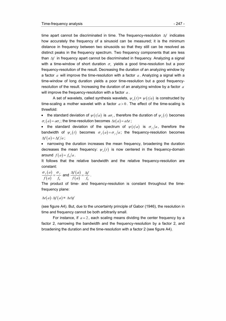
Time-frequency analysis - 247 -
time apart cannot be discriminated in time. The frequency-resolution f∆ indicateshow accurately the frequency of a sinusoid can be measured; it is the minimumdistance in frequency between two sinusoids so that they still can be resolved asdistinct peaks in the frequency spectrum. Two frequency components that are lessthan f∆ in frequency apart cannot be discriminated in frequency. Analyzing a signalwith a time-window of short duration tσ yields a good time-resolution but a poorfrequency-resolution of the result. Decreasing the duration of an analyzing window bya factor a will improve the time-resolution with a factor a . Analyzing a signal with atime-window of long duration yields a poor time-resolution but a good frequency-resolution of the result. Increasing the duration of an analyzing window by a factor awill improve the frequency-resolution with a factor a .
A set of wavelets, called synthesis wavelets, ( )a tψ = ( )t aψ is constructed bytime-scaling a mother wavelet with a factor 0a > . The effect of the time-scaling isthreefold:• the standard deviation of ( )t aψ is taσ , therefore the duration of ( )a tψ becomes
( )t ta aσ σ= ; the time-resolution becomes ( )t a a t∆ = ∆ ;• the standard deviation of the spectrum of ( )t aψ is f aσ , therefore thebandwidth of ( )a tψ becomes ( )f fa aσ σ= ; the frequency-resolution becomes
( )f a f a∆ = ∆ ;• narrowing the duration increases the mean frequency, broadening the durationdecreases the mean frequency: ( )a tψ is now centered in the frequency-domainaround ( ) 0f a f a= .It follows that the relative bandwidth and the relative frequency-resolution areconstant:
( )( ) 0
f faf a fσ σ
= and ( )( ) 0
f a ff a f∆ ∆
= .
The product of time- and frequency-resolution is constant throughout the time-frequency plane:
( ) ( )t a f a∆ ⋅∆ = t f∆ ∆
(see figure A4). But, due to the uncertainty principle of Gabor (1946), the resolution intime and frequency cannot be both arbitrarily small.
For instance, if 2a = , each scaling means dividing the center frequency by afactor 2, narrowing the bandwidth and the frequency-resolution by a factor 2, andbroadening the duration and the time-resolution with a factor 2 (see figure A4).

- 248 - Appendix
A continuous wavelet transform is defined as the decomposition locally attime t and frequency f of a signal ( )x t in V onto the analysing wavelets ( )ˆa tψ :
( )CWT ,f t = ( ) ( )*ˆax t dα ψ α α+∞
−∞−∫ ,
in which f and a are related by: 0a f f= . The square of the modulus of thecontinuous wavelet transform is called the scalogram of ( )x t :
( )CWT ,P f t = ( ) 2CWT ,f t .
f
t( )0 , 0
( )f a∆
( )t a∆level 3
level 1
level 2
level 4
0 2f
Figure A4. The time-frequency resolution of the wavelet transform is illustrated byrectangles in the time-frequency plane. Each rectangle has time-resolution
( )t a a t∆ = ∆ and frequency-resolution ( )f a f a∆ = ∆ . Each rectangle has constantarea t f∆ ∆ . At high frequencies, there is a better time-resolution and a poorerfrequency-resolution than at low frequencies. This means that two delta pulsescan be discriminated in time at high frequencies. Two sinusoids cannot bediscriminated in frequency at high frequencies. At low frequencies, time-resolutionis poorer but frequency-resolution is better. This means that two delta pulsescannot be discriminated in time at low frequencies. Two sinusoids can bediscriminated in frequency at low frequencies. 0f is the center of the motherwavelet in the frequency-domain. The levels are the levels of decomposition of thesignal into frequency bands.

Time-frequency analysis - 249 -
Because the continuous wavelet transform is a decomposition onto an orthogonalbasis, it follows that
( ) 2CWT ,f t df dt+∞ +∞
−∞ −∞∫ ∫equals the total energy of the signal ( )x t . This means that the scalogram
( ) 2CWT ,f t is a distribution of the energy of the signal in the time-frequency domainexpressed in power per frequency unit. The scalogram satisfies condition P1, butdoes not satisfy the marginal conditions P2 and P3 (see section 1).
Let 2a = and denote in this case the synthesis wavelets with ( )m tψ = ( )2mtψ ,for m∈ . The scaled wavelet ( )m tψ is centered around 0 2
mmf f= , the bandwidth is
( ) 2mf m f∆ = ∆ , and the duration is ( ) 2mt m t∆ = ∆ . Let ( )x t be a signal in V. Becausethe synthesis wavelets are localized in time at 0t = , we cannot decompose ( )x t ontothe set of synthesis wavelets ( )m tψ . But at each time 2mt k= , k is an integer, it ispossible to decompose ( )x t locally onto a set of time-shifted synthesis wavelets
( )2mm t kψ − , which are localized at 2mt k= . In other words, there exists a dualwavelet ( )ˆ tψ and dual analysis wavelets ( )ˆm tψ = ( )ˆ 2mtψ such that, for each signal( )x t in V, we can write:
( )x t = ( ), 2mm k mm k
c t kψ∞ ∞
=−∞ =−∞
−∑ ∑ , (A3)
with:
,m kc = ( ) ( )*ˆ 2mmx k dα ψ α α+∞
−∞−∫ . (A4)
The right hand side of equation (A3) is called the reconstruction of ( )x t . Thenumbers ,m kc are called wavelet coefficients. The right hand side of equation(A4) is called a wavelet transform of ( )x t :
( )WT ,m k = ( ) ( )*ˆ 2mmx k dα ψ α α+∞
−∞−∫ .
Note that this is a convolution of ( )x t with the function ( )ˆm tψ − . The scalogram:
( )WT ,P m k = ( ) 2WT ,m k =2
,m kc .
is the distribution of the energy of the signal in the time-frequency domain.In the case of a sampled signal, the wavelet transform produces a wavelet
coefficient ,m kc in each rectangle of figure A4. In this case m ranges from 1 to ∞ ,because the highest frequency is the sample frequency divided by 2. m is called thelevel of the decomposition. Figure A4 shows four levels. Each level coincides with afrequency band. Each level contains a signal component. We can use the waveletcoefficients of a level to reconstruct the signal component of that level, i.e., the signal

- 250 - Appendix
component of ( )x t in that frequency band. This requires the reconstruction of thethm -level component ( )mx t of ( )x t :
( )mx t = ( ), 2mm k mkc t kψ −∑ (A5)
Note that
( )x t = ( )1
mmx t
∞
=∑ .
Furthermore, an thm -level partial reconstruction ( )mx t of ( )x t can be made by:
( )mx t = ( )ii mx t
∞
=∑ ,
i.e., all the level components ( )ix t are summed up to the component of level m . Onecan say that the thm -level partial reconstruction is an approximation of the signalconsisting of the low frequency components up to the frequency component of levelm .
The literature on wavelet theory is very extensive. We mention only: Rioul etal. (1991), Hlawatsch et al. (1992), Chui (1992), Newland (ch.17, 1993), Akay (ch.8,1996), Qian et al. (ch.2 and 4, 1996), and Jensen et al. (2001).
An exampleFigure A6A presents an IBI-series of 128 s. The series is interpolated andequidistantly resampled with a sample frequency sF = 16 Hz, i.e., the number of dataN = 2048. The time-resolution t∆ = 0.0625 s. We want to analyze this time serieswith the wavelet transform. For this example we have chosen the Coiflet 2 waveletshown in figure A3B. This wavelet is scaled by the algorithm in such a way that theduration tσ = 0.0625 s, the bandwidth fσ = 8 Hz, and such that the wavelet iscentered around 0f = 12 Hz. Then the wavelet transform computes the waveletcoefficients ,m kc for a number of levels m .
For the first level, 1m = , the center frequency of the scaled wavelet ( )1 tψ is
1f = 0 2f = 6 Hz, the bandwidth ( )1fσ = 2fσ = 4 Hz, and the duration ( )1tσ = 2 tσ =0.125 s. This means that level 1 coincides with the frequency band 1B = [2,4] Hz. Thetime-resolution in this band is twice the original time-resolution, i.e., ( )1t∆ = 0.125 s,so the wavelet transform only computes 1N = / 2N wavelet coefficients 1,kc . For thesecond level, 2m = , 2f = 0 4f = 3 Hz, ( )2fσ = 4fσ = 2 Hz, ( )2tσ = 4 tσ = 0.25 s,
( )2t∆ = 0.25 s, and 2B = [2,4] Hz. The wavelet transform computes 2N = / 4Nwavelets coefficients 2,kc . Table A1 summarizes this for the first nine levels. In thistable, ( )t m∆ is not only the time-resolution of the frequency band mB , but also theduration of the wavelet mψ . Figure A5 shows the band-pass like power spectral

Time-frequency analysis - 251 -
densities of the scaled synthesis wavelets ( )5 tψ , ( )6 tψ , ( )7 tψ , and ( )8 tψ , withdecreasing center frequencies and decreasing bandwidths.
m mf ( )f m∆ ( )t m∆ mB mN1 6 4 0.125 [4,8] 10242 3 2 0.25 [2,4] 5123 1.5 1 0.5 [1,2] 2564 0.75 0.5 1 [0.5,1] 1285 0.375 0.25 2 [0.25,0.5] 646 0.1875 0.125 4 [0.125,0.25] 327 0.09375 0.0625 8 [0.0625,0.125] 168 0.046875 0.03125 16 [0.03125,0.0625] 89 0.0234375 0.015625 32 [0.015625,0.03125] 4
m 0 2mf 2mf∆ 2m t∆ ( ) ( ),
2 2m m
f m f mf f
∆ ∆ − +
2mN
Table A1. Summary of center frequencies, frequency-resolutions, time-resolutions,frequency bands, and number of points for 9 levels of decomposition.
Coiflet Wavelets (levels 5,6,7,8)
0 0.1 0.2 0.3 0.4 0.5 0.6frequency (Hz)
a.u.
level 8 level 7 level 6 level 5
Figure A5. The scaled synthesis Coiflet wavelets of levels 5, 6, 7, and 8 in thefrequency domain. The power spectral densities are band-pass like. Table A1 liststhe values of the increasing center frequencies and bandwidths.

- 252 - Appendix
Level 5: 0.25-0.5 Hz
00.20.40.60.8
1
0 16 32 48 64 80 96 112 128
B
Level 6: 0.125-0.25 Hz
00.20.40.60.8
1
0 16 32 48 64 80 96 112 128
C
Level 7: 0.0625-0.125 Hz
00.20.40.60.8
1
0 16 32 48 64 80 96 112 128
D
Level 8: 0.03125-0.0625 Hz
00.20.40.60.8
1
0 16 32 48 64 80 96 112 128
E
IBI
0.6
0.8
1
1.2
0 16 32 48 64 80 96 112 128time (s)
sA
Figure A6. The scalogram ( )WT ,P m k =2
,m kc for the levels m =5,6,7, and 8.
The Coiflet wavelet of figure A3 is used. A: the original IBI time series. We usedthe IBI-data of the Physiological Time-Frequency Analysis Package developed byHoutveen (2001). B,C,D,E: the 5th-, 6th-, 7th-, and 8th-level scalogram; they presentthe distribution of the energy of the signal in the frequency bands B5= [0.25,0.5],B6= [0.125,0.25], B7= [0.0625,0.125], and B8= [0.03125,0.0625] Hz, respectively.

Time-frequency analysis - 253 -
Level 5: 0.25-0.5 Hz
-0.3-0.2-0.1
00.10.20.3
0 16 32 48 64 80 96 112 1280.60.70.80.911.11.2
level 5IBI
A
Level 6: 0.125-0.25 Hz
-0.3-0.2-0.1
00.10.20.3
0 16 32 48 64 80 96 112 1280.60.70.80.911.11.2
level 6IBI
B
Level 7: 0.0625-0.125 Hz
-0.3-0.2-0.1
00.10.20.3
0 16 32 48 64 80 96 112 1280.60.70.80.911.11.2
level 7IBI
C
Level 8: 0.03125-0.0625 Hz
-0.3-0.2-0.1
00.10.20.3
0 16 32 48 64 80 96 112 1280.60.70.80.911.11.2
level 8IBI
D
Figure A7. Reconstructed components. The Coiflet wavelet of figure A3 is used.A,B,C,D: the 5th-, 6th-, 7th-, and 8th-level components of the signal in comparisonwith the original IBI time series. These components are the components of thesignal in the frequency bands B5= [0.25,0.5], B6= [0.125,0.25], B7= [0.0625,0.125],and B8= [0.03125,0.0625] Hz, respectively.

- 254 - Appendix
For each level m , the scalogram can be computed, using the waveletcoefficients of that level. The scalogram reflects the spectral density of the signal( )x t in the time-frequency domain at frequency 0 2
mmf f= , i.e., in frequency band
mB . For the levels 5, 6, 7, and 8 the scalograms are plotted in figures A6B, C, D, andE, respectively.
How does the signal component of ( )x t in the frequency band mB look like?For this we have to reconstruct the thm -level component ( )mx t of ( )x t , usingequation (A5). The 5th-, 6th-, 7th-, and 8th-level components are shown in figure A7A,B, C, and D, respectively. For instance, the 7th-level component is the component of( )x t in frequency band [0.0625,0.125] Hz, i.e., the 0.1 Hz rhythm. Finally, the 7th-
level partial reconstruction ( )7x t of ( )x t is shown in figure A8. One can say that( )7x t is equal to ( )x t without the high frequencies above 0.125 Hz.
Comparison with our methodThe method described in chapter 7 computes the instantaneous frequency of amonocomponent signal exactly at an optimal time-resolution. A monocomponentsignal is a signal that has only one (time-varying) spectral peak. The accuracy withwhich the frequency of a frequency component can be determined with a wavelettransform depends on the bandwidth fσ . If the frequency band ranges from 0.07 to0.15 Hz, i.e., the bandwidth is 0.08 Hz, a component of 0.1 Hz cannot be determinedaccurately in frequency. Due to the trade-off between duration and bandwidth, a
Level 7 partial reconstruction
0.6
0.8
1
1.2
0 16 32 48 64 80 96 112 128time (s)
s
signalreconstruction
Figure A8. Signal reconstruction. Shown is the 7th-level partial reconstruction ofthe original IBI time series. This approximation equals the signal without thefrequencies above 0.125 Hz.

Time-frequency analysis - 255 -
better frequency-resolution requires a longer time-interval. Therefore, the wavelettransform cannot reach the accuracy of our method.
Figure A5 shows the frequency transfer functions on a linear frequency andamplitude scale of the Coiflet wavelets at levels 8, 7, 6, and 5, i.e., a wavelet filter-bank. Their center frequencies and bandwidths increase each time with a factor 2(see the table above). Our filter-bank of cos2-shaped filters was designed conformthe physiological definitions of the HRV components, with ‘unity-gain’ behavior, andan optimal f tσ σ product according to Gabor (see chapter 7). Comparing these twofilter-banks, we can make the following comments.• The wavelet filter-bank does not show ‘unity-gain’ behavior.• The filters of the wavelet filter-bank show an overshoot in their pass-bands of60%, so depending on the frequency of the components, they will be substantiallyattenuated or affected, whereas our filters have an overshoot better than 0.1%.• Also in the stop-band of the wavelet filters, there is an attenuation of only 40 dB(1%), so various components will still show minor leakage from adjacent filters; theattenuation in the stop-band of our filters is better than 80 dB.
There is also a remark of a fundamental nature. It is emphasized here thatonly the squared modulus (or ‘power-density’) of the wavelet transform is utilized (i.e.,the scalogram, figure A6). It can be compared to the square of our instantaneousamplitude (see chapter 7). In our method, we also utilize the phase informationcontained in the complex analytical signals to yield the instantaneous frequency andbandwidth. The latter is extensively explored regarding its potential to separateoscillatory and irregular (‘noisy’) periods of the signal over time (chapters 7, 8, and 9).
4 Cohen’s general class of time-frequency representations
This section reviews an approach based on the characterization of time-frequencyrepresentations by means of a kernel-function. By constructing special kernel-functions one can produce representations with desirable properties. This led toCohen’s general class of time-frequency representations.
4.1 The Wigner-Ville distribution
The Wiener-Khinchine theorem states that the power spectral density ( )S f of astationary stochastic process ( )x t is the Fourier transform of the auto-correlationfunction ( )R τ of the process (e.g., Bendat et al. p:121, 1986):
( )S f = ( )fF Rτ τ→ = ( ) 2 jfR e dπ ττ τ+∞ −
−∞∫ .

- 256 - Appendix
To compute the power spectral density of an HRV-signal, this signal has to bestationary. What if an HRV-signal is not stationary? If a signal is not stationary, onehas to consider the time-dependent auto-correlation and power spectral densityfunctions. The time-dependent auto-correlation function of an analytical signal ( )s t(see the appendix of chapter 6) is defined as the product of two points of the signallying symmetrically around time t at distance 2τ (e.g., Qian et al. p:104, 1996;Bendat et al. p:456, 1986):
( ),R t τ = *ˆ ˆ2 2
s t s tτ τ + ⋅ −
in which τ is called the time-shift or time-lag variable. The time-dependent auto-correlation function is also called local auto-correlation function (Cohen p:137, 1995)or instantaneous auto-correlation function (Steeghs p:30, 1997; Williams p:8, 1997).
The Fourier transform of the local auto-correlation function with respect to thetime-shift variable τ is called the Wigner-Ville distribution (Wigner, 1932; Ville,1948):
( )WVD ,t f = ( ),fF R tτ τ→ = ( ) 2, jfR t e dπ ττ τ+∞ −
−∞∫ .
For a discussion of the Wigner-Ville distribution see for instance Claasen et al.(1980a; 1980b; 1980c), Boashash (1991; 1992), Cohen (ch.8, 1995), Qian et al.(ch.5, 1996), and Steeghs (pp:29-47, 1997). The Wigner-Ville distribution isinterpreted as a power spectral density function, representing the power of the signal( )x t for each point ( ),t f of the time-frequency plane. The Wigner-Ville distribution
satisfies the marginal conditions P2 and P3 and the total power of the Wigner-Villedistribution in the time-frequency plane equals the total power of the signal.Furthermore, the Wigner-Ville distribution satisfies condition P4: it is possible to usethe Wigner-Ville distribution to compute the instantaneous frequency of the signal(see chapters 7 and 8).
4.2 Cross-terms
The Wigner-Ville distribution is not a true density because it may become negativedue to cross-terms: the Wigner-Ville distribution does not satisfy condition P1. Thecross-terms are due to the bilinear nature of the Wigner-Ville distribution (seeequation A14). Suppose ( )ts consists of two independent pure sinusoids withdifferent frequencies 2 1f f> :
( )ts = 12 jf te π + 22 jf te π .
The Wigner-Ville distribution of this analytical function is:

Time-frequency analysis - 257 -
( )WVD ,t f = ( )1f fδ − + ( )2f fδ − + ( ) ( )2 cos 2h df f f tδ − ⋅ (A6)
in which ( )1 2 2hf f f= + , ( )2 1 2df f f= − , and ( )δ ⋅ is the Dirac delta-function. Thefirst two terms on the right hand side of (A6) are the auto-terms associated with thetwo sinusoids. The third term is a so-called cross-term. In the time-frequency plane, itis located halfway between the two auto-terms at frequency ( )1 2 2hf f f= + . Thecross-term is a sinusoid with frequency ( )2 1 2df f f= − , i.e., the difference of thefrequencies of the two original sine waves. The same applies to two delta-functions intime at different instants 2 1t t> :
( )s t = ( )1t tδ − + ( )2t tδ − .
The Wigner-Ville distribution of ( )s t is:
( )WVD ,t f = ( )1t tδ − + ( )2t tδ − + ( ) ( )2 cos 2h dt t ftδ π− ⋅ (A7)
in which ( )1 2 2ht t t= + and ( )2 1 2dt t t= − . The first two terms on the right hand side of(A7) are the auto-terms associated with the two events in time. The third term is a so-called cross-term. In the time-frequency plane, it is located halfway between the twoauto-terms at time ( )1 2 2ht t t= + . The cross-term is a sinusoid with frequency
( )2 1 2dt t t= − .This means that between each two frequency components (time components)
present in a signal, there appears a cross-term in the time-frequency plane. They canalso occur at the location of the auto-terms. One can say that cross-terms areundesirable because they obscure the Wigner-Ville distribution and make it difficult tointerpret the distribution. Therefore, one may want to suppress the cross-terms. Theambiguity function plays a role in suppressing the cross-terms of the Wigner-Villedistribution. This is discussed in the next sections. However, if the Wigner-Villedistribution is used to compute signal-parameters one may need the cross-terms;suppressing the cross-terms may lead to incorrect outcomes. An example of aWigner-Ville distribution with cross-terms is given in figure 4 of chapter 5. Cross-terms are discussed in chapters 5 and 6, and for instance by Cohen (pp:124-127,1995), Qian et al. (pp:112-118, 1996). Though very small, the spectrogram and thescalogram include also cross-terms (Kadambe et al., 1992; Kootsookos et al., 1992).
4.3 The ambiguity function
The inverse Fourier transform of the local auto-correlation function with respect to thetime variable is called the ambiguity function (e.g., Boashash p:437, 1991; Cohenp:96, 1995; Qian et al. p:132, 1996; Steeghs p:36, 1997):
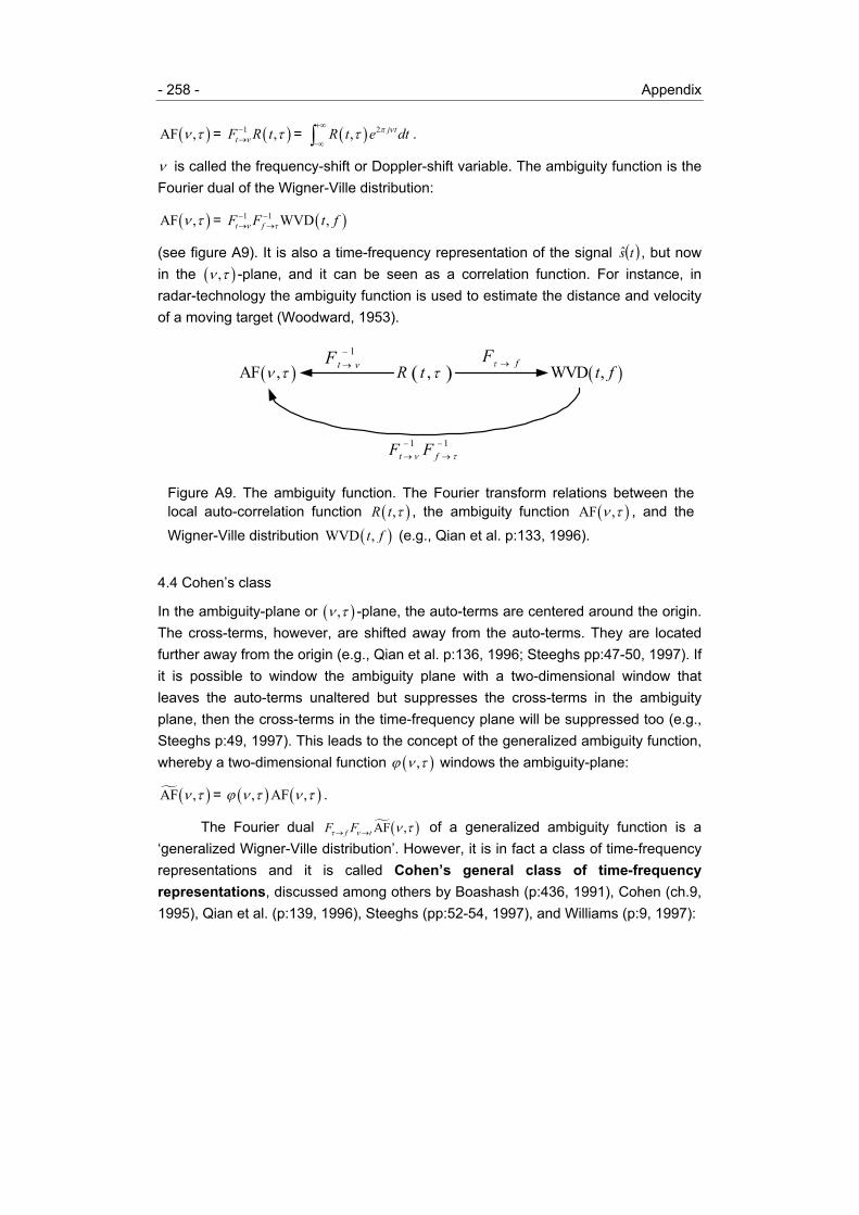
- 258 - Appendix
( )AF ,ν τ = ( )1 ,tF R tν τ−→ = ( ) 2, j tR t e dtπ ντ
+∞
−∞∫ .
ν is called the frequency-shift or Doppler-shift variable. The ambiguity function is theFourier dual of the Wigner-Ville distribution:
( )AF ,ν τ = ( )1 1 WVD ,t fF F t fν τ− −→ →
(see figure A9). It is also a time-frequency representation of the signal ( )ts , but nowin the ( ),ν τ -plane, and it can be seen as a correlation function. For instance, inradar-technology the ambiguity function is used to estimate the distance and velocityof a moving target (Woodward, 1953).
4.4 Cohen’s class
In the ambiguity-plane or ( ),ν τ -plane, the auto-terms are centered around the origin.The cross-terms, however, are shifted away from the auto-terms. They are locatedfurther away from the origin (e.g., Qian et al. p:136, 1996; Steeghs pp:47-50, 1997). Ifit is possible to window the ambiguity plane with a two-dimensional window thatleaves the auto-terms unaltered but suppresses the cross-terms in the ambiguityplane, then the cross-terms in the time-frequency plane will be suppressed too (e.g.,Steeghs p:49, 1997). This leads to the concept of the generalized ambiguity function,whereby a two-dimensional function ( ),ϕ ν τ windows the ambiguity-plane:
( )AF ,ν τ = ( ) ( ), AF ,ϕ ν τ ν τ .
The Fourier dual ( )AF ,f tF Fτ ν ν τ→ → of a generalized ambiguity function is a‘generalized Wigner-Ville distribution’. However, it is in fact a class of time-frequencyrepresentations and it is called Cohen’s general class of time-frequencyrepresentations, discussed among others by Boashash (p:436, 1991), Cohen (ch.9,1995), Qian et al. (p:139, 1996), Steeghs (pp:52-54, 1997), and Williams (p:9, 1997):
( )AF ,ν τ ( )WVD ,t f( ),R t τ1
tF ν−→ fFτ →
1 1t fF Fν τ− −→ →
Figure A9. The ambiguity function. The Fourier transform relations between thelocal auto-correlation function ( ),R t τ , the ambiguity function ( )AF ,ν τ , and theWigner-Ville distribution ( )WVD ,t f (e.g., Qian et al. p:133, 1996).

Time-frequency analysis - 259 -
( ),t fρ = ( ) ( )1, ,f t tF F F R tτ ν νϕ ν τ τ−→ → → = ( ) ( ) 2 2 2, , j u jt jfR u e dud dπ ν π ν π τϕ ν τ τ ν τ
+∞ +∞ +∞ + − −
−∞ −∞ −∞∫ ∫ ∫
(see figure A10).
The two-dimensional window ( ),ϕ ν τ of the ambiguity-plane is referred to as thekernel of the time-frequency representation (e.g., Claasen et al., 1980c; Steeghsp:54). The Wigner-Ville distribution belongs to Cohen’s general class and has kernel( ),ϕ ν τ = 1. Other time-frequency representations belonging to Cohen’s general class
are the spectrogram with kernel
( ),ϕ ν τ = * 2
2 2j uw u w u e duπ ντ τ+∞ −
−∞
+ − ∫
in which ( )w t is the window function (see section 2), and the Rihaczek distribution(Rihaczek, 1968) with kernel
( ),ϕ ν τ = 2je πντ ,
(e.g., Boashash, p:434, 1991; Cohen p:138, 1995; Williams p.7, 1997).The first approach to suppress the cross-terms was the application of a
‘smooth’-kernel. The cross-terms were suppressed by smoothing the Wigner-Villedistribution with a two-dimensional filter. This resulting representation is called asmoothed Wigner-Ville distribution (see chapter 5) (e.g., Boashash p:472, 1991;Novak, 1993a). Choi et al. (1989) applied an exponential kernel:
( ),ϕ ν τ = 2 2
e ν τ σ− .
( )AF ,ν τ
( ),t fρ
( ),R t τ1
tF ν−→ fFτ →
( ),R t τtFν →( ),ϕ ν τ ⊗
( )AF ,ν τ
( )WVD ,t f
fFτ →
Figure A10. Cohen’s general class of time-frequency representations. The Fouriertransform relations between the generalized local auto-correlation function ( ),R t τ ,
the generalized ambiguity function ( )AF ,ν τ , and Cohen’s general class of time-frequency representations (e.g., Cohen pp:136-139, 1995).

- 260 - Appendix
The generalized distribution with this kernel is called the exponential distribution(see chapter 6).
To satisfy the ‘desirable’ conditions of time-frequency representations (section1) the kernel ( ),ϕ ν τ is subject to various restrictions and not every kernel can beapplied. By constructing special kernel-functions with special constraints one canproduce representations with prescribed, desirable properties. The construction ofspecial kernels was also inspired by the question how to get rid of the cross-terms inthe Wigner-Ville distribution. This leads to the so-called cross-term reducing ‘cone-kernel’ applied in the ZAM-distribution, and a class of cross-term reducing ‘bowtie’shaped kernels. Members of Cohen’s class that have cross-term reducing kernelsare called reduced interference distributions. These are discussed for instance by:Boashash (pp:438,445-451, 1991), Zhao et al. (1991), Hlawatsch et al. (p:41, 1992),Kootsookos et al. (1992), Cohen (pp:141-149, 1995), and Williams (pp:8-20, 1997).
4.5 Applications
Novak et al. (1993a; 1993b; 1999) used time-frequency methods based on a Wigner-Ville distribution to graphically inspect the time-varying frequency contents and thecross time-frequency representation of and between cardiorespiratory signals. Polaet al. (1996) computed the power spectral density of HRV during autonomic tests (tilttest, phenylephrine administration, and Valsalva manoeuvre) by means of severaltime-frequency methods. They included the spectrogram, a smoothed Wigner-Villedistribution, and the exponential distribution. The spectrogram does not satisfy themarginal conditions. It may have a good time-resolution, though. However, thespectrogram is not very accurate in describing transients, because the time-resolution is dependent on the time-window. The smoothed Wigner-Ville distributionand the exponential distribution have a good time-resolution and both can detecttransients with an accuracy of a few samples. Furthermore, a local power spectraldensity may be estimated, but results are dependent on the suppression of the cross-terms.
5 Other time-frequency representations
A fixed kernel is not capable of suppressing all the cross-terms in the ambiguityplane. Under the condition that the auto-terms and the cross-terms are separated inthe ambiguity plane, Baraniuk et al. (1993a) developed an adaptive algorithm thatsuppresses the cross-terms that lie away from the auto-terms. This means that thealgorithm produces an adaptive kernel that is 1 in the region of the auto-terms that lie

Time-frequency analysis - 261 -
around the origin of the ambiguity plane, 0 outside this region, and has smoothedges. The ambiguity function is multiplied with this kernel and the resulting time-frequency representation (i.e., the Fourier dual) is called the adaptive optimalkernel time-frequency representation (Baraniuk et al., 1993a; 1993b; 1994; Joneset al., 1995). In fact, the adaptive optimal kernel is signal dependent. Therefore thisrepresentation does not belong to Cohen’s general class. However, it is expectedthat this dependency guarantees a good performance for a broad class of signals,because the locations of the auto- and cross-terms depend on the signal (Baraniuk etal., 1993b). The adaptive optimal kernel time-frequency representation generallydoes not satisfy the conditions of an ideal time-frequency representation, forinstance, the marginal conditions. Furthermore, it may not be possible to derive theinstantaneous frequency because it contains no phase information. It may still beinteresting to apply this representation because of the very good visualization of thetime-varying fluctuations in HRV. Pattern recognition analysis may be applied to theadaptive optimal kernel time-frequency representation to identify and describeclusters of activity in the time-frequency plane.
The Gabor representation is a decomposition of the signal onto a basis oftime-shifted and frequency modulated Gaussian functions (compare this with theshort-time Fourier transform and the wavelet transform) (e.g., Hlawatsch et al. pp:28-29, 1992; Qian et al. p:52, 1996).
Another time-frequency representation is the fast time-frequency transformand its general formulation, the discrete time-frequency transform (Martens, 1992;1999). This algorithm is the joint computation of the instantaneous amplitude andinstantaneous frequency of an analytical signal in certain predefined narrowfrequency bands. After filtering the signal, the instantaneous amplitude is themodulus of the resultant analytical signal, and the instantaneous frequency isestimated by means of the argument of the local auto-correlation function of thesignal (see chapter 8).
References
Akselrod S, Oz O, Greenberg M, and Keselbrener L. Autonomic response to changeof posture among normal and mild-hypertensive adults: investigation by time-dependent spectral analysis. J Autonomic Nervous System 64:33-43, 1997.
Akay M. Detection and estimation methods for biomedical signals. San Diego CA:Academic Press Inc, 1996, ISBN 0120471434.

- 262 - Appendix
Baraniuk RG and Jones DL. A signal-dependent time-frequency representation:optimal kernel design. IEEE Trans Signal Proc SP-41(4):1589-1602, 1993a.
Baraniuk RG and Jones DL. Signal-dependent time-frequency analysis using aradially Gaussian kernel. Signal Proc 32:263-284, 1993b.
Baraniuk RG and Jones DL. A signal-dependent time-frequency representation: fastalgorithm for optimal kernel design. IEEE Trans Signal Proc SP-42(1):134-145,1994.
Bendat JS and Piersol AG. Random Data, Analysis and Measurements Procedures,2nd edition. New York: John Wiley and Sons, Inc., 1986.
Boashash B. Time-frequency signal analysis. In: Advances in Spectrum Analysis andArray Processing, Vol. 1. S. Haykin, Ed. Englewood Cliffs, NJ: Prentice Hall,pp:418-517, 1991.
Boashash B. Estimating and interpreting the instantaneous frequency of a signal –part 1: fundamentals. Proc IEEE 80(4):520-538, 1992.
Choi HI and Williams WJ. Improved time-frequency representation of multicomponentsignals using exponential kernels. IEEE Trans Acoust Speech, SignalProcessing ASSP-37:862-871, 1989.
Chui CK. An Introduction to Wavelets. New York: Academis Press, 1992.Claassen TACM and Mecklenbräuker WFG. The Wigner distribution - a tool for time-
frequency signal analysis, part I: continuous-time signals. Philips Res J 35:217-250, 1980a.
Claassen TACM and Mecklenbräuker WFG. The Wigner distribution - a tool for time-frequency signal analysis, part II: discrete-time signals. Philips Res J 35:276-300, 1980b.
Claassen TACM and Mecklenbräuker WFG. The Wigner distribution - a tool for time-frequency signal analysis, part III: relations with other time-frequency signalanalysis. Philips Res J 35:372-389, 1980c.
Cohen L. Time-Frequency Analysis. Englewood Cliffs, NJ: Prentice Hall Inc, 1995,ISBN 0135945321.
Gabor D. Theory of communication. Proc IEE 93(III):429-457, 1946.Hlawatsch F and Boudreaux-Bartels GF. Linear and quadratic time-frequency signal
representations. IEEE Sig Proc Magazine 9:21-67, 1992.Houtveen JH. Psychological and physiological responses to stress (Ph.D. Thesis).
Amsterdam: University of Amsterdam, 2001.Jensen A and la Cour-Harbo A. Ripples in Mathematics – The Discrete Wavelet
Transform. Berlin-Heidelberg-New York: Springer-Verlag, 2001, ISBN3540416625.

Time-frequency analysis - 263 -
Jones DL and Baraniuk RG. An adaptive optimal-kernel time-frequencyrepresentation. IEEE Trans Signal Proc SP-43(10):2361-2371, 1995.
Kadambe S and Boudreaux-Bartels G. A comparison of the existence of ‘cross terms’in the Wigner distribution and the squared magnitude of the wavelet transformand the short time Fourier transform. IEEE Trans Acoust Speech Signal Proc40(10):2498-2517, 1992.
Keselbrener L and Akselrod S. Selective discrete Fourier transform algorithm fortime-frequency analysis: method and application on simulated andcardiovascular signals. IEEE Trans Biomed Eng BME-43(8):789-802, 1996.
Kootsookos PJ, Lovell BC, and Boashash B. A unified approach to the STFT, TFDsand instantaneous frequency. IEEE Trans. Signal Processing 40:1971-1982,1992.
Martens WLJ. The fast time frequency transform (F.T.F.T.): a novel on-line approachto the instantaneous spectrum. 14th International Conference of the IEEEEngineering in Medicine and Biology Society, 1992, Paris.
Martens WLJ. Segmentation of ‘rhythmic’ and ‘noisy’ components of sleep EEG,heart rate and respiratory signals based on instantaneous amplitude, frequency,bandwidth and phase. 1st joint BMES/EMBS conference 1999, Atlanta.
Newland DE. An Introduction to Random Vibrations, Spectral and Wavelet Analysis,3rd edition. New York: Longman Scientific & Technical, 1993, ISBN0582215846.
Novak P and Novak V. Time/frequency mapping of the heart rate, blood pressure andrespiratory signals. Medical & Biological Engineering & Computing 31(2):103-110, 1993a.
Novak V and Novak P, de Champlain J, Le Blanc AR, Martin R, and Nadeau R.Influence of respiration on heart rate and blood pressure fluctuations. Journal ofApplied Physiology 74(2):617-626, 1993b.
Novak V, Reeves AL, Novak P, Low PA, and Sharbrough FW. Time-frequencymapping of R-R interval during complex partial seizures of temporal lobe origin.Journal of the Autonomic Nervous System 77(2-3):195-202, 1999.
Pola S, Macerata A, Emdin M, and Marchesi C. Estimation of the power spectraldensity in nonstationary cardiovascular time series: assessing the role of thetime-frequency representations (TFR). IEEE Trans Biomed Eng BME-43(1):46-59, 1996.
Qian S and Chen D. Joint time-Frequency Analysis – Methods and Applications.Upper Saddle River, NJ: Prentice Hall Inc, 1996, ISBN 0132543842.

- 264 - Appendix
Rihaczek A. Signal energy distribution in time and frequency. IEEE Trans. Inform.Theory IT-14:369-374, 1968.
Rioul O and Vetterli M. Wavelets and signal processing. IEEE Sig Proc Magazine9:14-38, 1991;
Steeghs P. Local power spectra and seismic interpretation (Ph.D. Thesis). Delft: DelftUniversity of Technology, 1997.
Ville J. Théorie et application de la notion de signal analytique. Cables etTransmissions 2A(1):61-74, 1948.
Wigner E. On the quantum correction for thermodynamic equilibrium. Phys Rev40:749-759, 1932.
Williams WJ. Recent advances in time-frequency representations: some theoreticalfoundations. In: Time frequency and wavelets in biomedical signal processing.Akay M (ed). John Wiley & Sons, Inc. pp:3-43, 1997, ISBN: 0780311477
Woodward PM. Probability and information theory with application to radar. London:Pergamon Press, 1953.
Zhao Y, Atlas E, and Marks RJ. The use of cone-shaped kernels for generalizedtime-frequency representations on nonstationary signals. IEEE Trans AcoustSpeech Signal Processing ASSP-38:1084-1091, 1990.

Glossary - 265 -
Glossary
AliasingThis is an error that occurs when the sampling frequency is lower than twice thehighest frequency contained in the signal.
Ambiguity functionThe inverse Fourier transform of the local auto-correlation function with respect tothe time variable is called the ambiguity function:
( )AF ,ν τ = ( )1 ,tF R tν τ−→ = ( ) 2, j tR t e dtπ ντ
+∞
−∞∫ ,
ν is called the frequency-shift or Doppler-shift variable. The ambiguity function playsa role in suppressing the cross-terms of the Wigner-Ville distribution.
Analytic(al) signalAn analytical signal is a signal that has no negative frequency components,equivalently, a signal of which the Fourier transform is equal to 0 for frequencieslower than 0. The analytical signal ( )ts associated with a real signal ( )x t allows us todefine the instantaneous amplitude, instantaneous phase, and instantaneousfrequency of the real signal ( )x t .
Autocorrelation functionThe autocorrelation function of a complex signal ( )s t is defined by:
( ) ( ) ( )R s t s t dtτ τ+∞ ∗
−∞= +∫
This is a measure of the dependence of a value of a signal at one time on the valuesof the signal at another time. The autocorrelation function may be used to detect adeterministic component masked in a random background, because theautocorrelation function of deterministic data persist over all time displacements,while the autocorrelation function of stochastic processes tends to zero if the timedisplacement becomes large (for zero-mean time series).
Auto-termAn auto-term represents the power in the time-frequency plane of a frequency-component or a time-component present in a signal.

- 266 - Appendix
Cardiac event seriesA cardiac event series is an HRV-representation obtained by representing each R-wave by a narrow positive spike of constant unit area generated at the R-waveoccurrence time.
Central Finite DifferenceA discrete estimator of the instantaneous frequency is the discrete derivative of thephase [ ]nϕ of the discrete analytical time series [ ] [ ] [ ]njenans ϕ=ˆ . The estimator is thesymmetrical discrete derivative:
[ ] [ ] [ ]( )
12 2 1i
s
n k n kf n
k tϕ ϕ
π + − −
= ⋅ + .
( st is the sample interval.) The discrete differentiation of [ ]nϕ must be obtained bysubtracting phases at uncorrelated points [ ]n kϕ + and [ ]n kϕ − .
Characteristic frequency components, bands, or rhythmsIn the range of short-term variability, three bands can often be distinguished in the
power spectrum at frequencies near 0.04, 0.1, and 0.3 Hz. The first band, at 0.04Hz, is of uncertain origin. The 0.1 Hz band is probably mediated by the baroreflexand reflects the variable sympathetic and parasympathetic tone of the autonomicnervous system. The band near 0.3 Hz may reflect parasympathetic (vagal) tonelinked with respiration. In the study of HRV, these bands are called the characteristicfrequency components, bands, or rhythms.
Circular mean directionAn estimate of the instantaneous frequency is the circular mean direction of the
discrete Wigner-Ville distribution:
[ ] [ ]1
2 /
0
/ 2 arg ,2
Nj k Ns
ik
Ff n W n k e π
π
−⋅
=
= ⋅ ⋅∑
Cross-termA limitation of the Wigner-Ville distribution is the appearance of cross-terms. Theyare sinusoidal components that appear between two auto-terms. This means thatbetween two frequency-components that are simultaneously present in a time-interval or between two time-components that are both present in a frequency-interval, there appears a cross-term in the time-frequency plane. The cross-terms are

Glossary - 267 -
due to the bilinear nature of the Wigner-Ville distribution. One can say that cross-terms are undesirable because they obscure the Wigner-Ville distribution and make itdifficult to interpret the distribution.
Discrete time-frequency transformThe discrete time-frequency transform is the general formulation of the fast time-frequency transform.
Discrete Wigner-Ville distributionThe discrete Wigner-Ville distribution of an discrete analytical time series [ ]s n ,
0,..., 1n N= − is defined by:
[ ] [ ] [ ]1
1
* 4 /ˆ ˆ,N
j ik N
i NW n k s n i s n i e π− ⋅
=−
= + − ⋅∑
in which 1 2N N= .
ECGThe electrocardiogram.
EnvelopeInstantaneous amplitude.
Fast time-frequency transformThis algorithm is the joint computation of the instantaneous amplitude andinstantaneous frequency of an analytical signal ( )ts in certain predefined narrowfrequency bands. After filtering the signal, the instantaneous amplitude is themodulus of the resultant analytical signal, and the instantaneous frequency isestimated by means of the argument of the local auto-correlation function of thesignal ( )ts .
( ) ( )ˆˆ1 arg ,12i ssf t R tπ
≈
Fourier analysisBy means of Fourier analysis, a time-domain function ( )x t can be investigated in thefrequency-domain. This is also called spectral analysis. A function ( )x t can bewritten as a sum of sinus-functions, each with a specific amplitude and frequency.

- 268 - Appendix
There is a ono-to-one relationship between amplitudes and frequencies and thisrelationship represents the function as a function of frequency. This transforms thefunction from the time-domain to the frequency-domain and is called the Fouriertransform. The square of the absolute value of the amplitude of a sinusoid is ameasure of the power of the sinusoid. Therefore, the absolute values of theamplitudes are often squared. The result, as function of the frequency, is called the
power spectrum.
Fourier transformThe Fourier transform ( )X f of a real or complex function ( )x t is defined by:
( ) ( ) 2 jftX f x t e dtπ+∞ −
−∞= ∫ .
See also Fourier analysis.
Frequency resolutionThe frequency-resolution f∆ indicates how accurately the frequency of a sinusoidcan be measured; it is the minimum distance in frequency between two sinusoids sothat they still can be resolved as distinct peaks in the power spectrum. Twofrequency components that are less than f∆ in frequency apart cannot bediscriminated in frequency.
Heart rateHeart rate is the number of heartbeats per unit time, conventionally, per minute.
Heart rate event seriesThe spikes of a cardiac event series represent the R-wave occurrence times. Eachspike is weighed with the inverse of the value of the interbeat interval obtained at thatR-wave occurrence time, multiplied with the duration of the preceding R-R interval.The result is called the heart rate event series.
Heart rate variability (HRV)The beat-to-beat fluctuations in heart rate are called heart rate variability.
HRVHeart rate variability.

Glossary - 269 -
HRV-representationA representation of HRV is defined as the beat-to-beat information derived fromthe ECG and ordered in such a way that it is accessible to the analysis techniquesand can be related to physiological processes.
InstantaneousInstantaneous signal properties are properties that can be computed within the time-resolution of the signal. Computations of a property over a shorter time interval yieldadjacently dependent values in time; if computed over a longer time interval, thevalues will be averaged.
Instantaneous amplitudeLet ( ) ( ) ( )ˆ j ts t a t e ϕ= be an analytical signal. The instantaneous amplitude orenvelope is the modulus ( )ta of ( )ts . The squared instantaneous amplitude is ameasure of the time-varying instantaneous power or energy per unit time of thesignal within a narrow frequency band.
Instantaneous bandwidthThe instantaneous frequency defines the time-varying frequency location of thespectral peak within a narrow frequency band. Due to a stochastic component, thespectral peak can have a spread. The instantaneous frequency is the average of thespread. The width (in the frequency direction) of the spread of the spectral peak ismeasured by means of the instantaneous bandwidth, being the associated standarddeviation of the average instantaneous frequency.
Instantaneous bandwidth coefficientThe so-called instantaneous bandwidth coefficient is computed by our method as ameasure of the instantaneous bandwidth. The instantaneous bandwidth coefficientmay serve as a time-varying segmentator of oscillatory versus irregular periods: lowvalues indicate oscillatory properties, high values indicate irregularities.
Instantaneous frequencyLet ( ) ( ) ( )ˆ j ts t a t e ϕ= be an analytical signal. The instantaneous frequency ( )if t isdefined as the derivative of the instantaneous phase ( )tϕ of ( )ts :
( ) ( )tdtdtfiϕ
π21
= .

- 270 - Appendix
The instantaneous frequency defines the time-varying frequency location of thespectral peak within a narrow frequency band. Due to a stochastic component, thespectral peak can have a spread. The instantaneous frequency is the average of thespread. The width of the spread is called the instantaneous bandwidth.
Instantaneous heart rateThis is the reciprocal of an interbeat interval.
Instantaneous heart rate spectrumThis is a power spectrum of a heart rate event series.
Instantaneous phaseLet ( ) ( ) ( )ˆ j ts t a t e ϕ= be an analytical signal. The instantaneous phase is defined asthe argument ( )tϕ of ( )ts .
Instantaneous spectrumThe time-varying power spectrum of a signal that can be computed within the
time-resolution of the signal.
Interbeat intervalTime duration between two consecutive R-waves in the ECG.
Integral pulse frequency modulation modelSystem that transforms a continuous input signal into an event series.
Local autocorrelation functionThe local auto-correlation function (also called: time-dependent or instantaneousauto-correlation function) of an analytical signal ( )s t is defined as the product oftwo points of the signal lying symmetrically around time t at distance 2τ :
( ),R t τ = *ˆ ˆ2 2
s t s tτ τ + ⋅ −
,
in which τ is called the time-shift or time-lag variable.

Glossary - 271 -
Low-pass filtered cardiac event seriesThe low-pass filtered cardiac event series is an HRV-representation that is derivedfrom a cardiac event series. This spike-train of a cardiac event series is filteredwith a zero-phase low-pass filter. Often a cutoff frequency of 0.5 Hz is used. Thefiltered continuous-time signal is called the low-pass filtered cardiac event series.After sampling this signal the resulting equidistant time series can be used for furthercomputations.
MonocomponentA monocomponent signal is a signal that has only one (time-varying) spectral band.
MulticomponentA signal is multicomponent means that the signal’s energy is locally distributed in twoor more frequency bands.
Non-stationaryA signal is said to be non-stationary, if it has time-varying statistical properties.Suppose a signal is divided in segments and for each segment a statistic iscomputed. Possibly, the statistics differ from segment to segment. When thedifferences are significant, the signal is called non-stationary.
Power spectrumPower spectral density.
Power spectral density (function)The power spectral density or power spectrum describes how the power (or variance)of a time series is distributed with frequency. See also Fourier analysis.
R-R intervalInterbeat interval.
SamplingExtraction of discrete numeric data from an analog continuous signal.
Sampling frequencyRate of extraction of discrete numeric data from an analog continuous signal.

- 272 - Appendix
Short-term variabilityThe beat-to-beat fluctuations in heart rate present in periods up to several minutes(2-5 min) are called short-term variability.
Spectral analysisFourier analysis.
Spectrum of countsA spectrum of counts is the power spectrum of a cardiac event series.
StationarySee non-stationary.
Time-frequency representationA distribution that represents the power of a signal simultaneously in time andfrequency is called a (joint) time-frequency representation. Time-frequencydistributions are used to study non-stationary signals: they give a spectralrepresentation of the signal which is function of time.
Time resolutionThe time-resolution t∆ indicates how accurately in time an event can be measured; itis the minimum difference in time between two peaks so that they still can beresolved as distinct peaks in time. Two delta pulses that are less than t∆ in timeapart cannot be discriminated in time.
Time sliceA time-slice tT at time t of a time-frequency distribution ( ),T t f is defined by
tT = ( ){ }, , allT t f f . Each time-slice can be viewed as an instantaneous spectrum.
Uncertainty principle of GaborGabor stated that, for a given filter, the product of the width in the time-domain tσand the width in the frequency-domain fσ is greater than or equal to 1 4π . Inequation: 1 4t fσ σ π⋅ ≥ . This means that, the wider (or narrower) the bandwidth of afilter is, the shorter (or longer) the corresponding impulse response is in the time-domain. The minimal product is reached for a normal distribution, which is aGaussian shaped filter. Any other filter shape will deviate from a minimal product.

Glossary - 273 -
Wigner-Ville distributionThe Wigner-Ville distribution is a time-frequency representation defined as the
Fourier transform of the local auto-correlation function with respect to the time-shift variable τ :
( )WVD ,t f = ( ),fF R tτ τ→ = ( ) 2, jfR t e dπ ττ τ+∞ −
−∞∫ .
Zero-phase filterA filter that cannot change the phase of a signal.
Reference
Working Group on Blood Pressure and Heart Rate Variability of the EuropeanSociety of Hypertension. Glossary of terms used in time series analysis ofcardiovascular data. Http://www.cbi.polimi.it/glossary/glossary.html

- 274 - Appendix
Abbreviations
ACF autocorrelation functionAM amplitude modulationBP blood pressureCFD central finite differenceCMD circular mean directionCZT chirp Z-transformCWT color word testDBP diastolic blood pressureDED discrete exponential distributionDFT discrete Fourier transformDPACF discrete pseudo autocorrelation functionDTFT discrete time frequency transformDWVD discrete Wigner-Ville transformECG electrocardiogramED exponential distributionFFT fast Fourier transformFM frequency modulationFTFT fast time frequency transformHR heart rateIBI interbeat intervalIHRS instantaneous heart rate spectrumIPFM integrated pulse frequency modulationLPFCES low-pass filtered cardiac event seriesPAF pure autonomic failurePSD power spectral densityRSP respirationSBP systolic blood pressureSOC spectrum of countsSTFT short-time Fourier transformTFD time-frequency distributionTFR time-frequency representationUTS uncorrelated time slicesWD Wigner transformWVD Wigner-Ville transform

DANKWOORDCURRICULUM VITAELIST OF PUBLICATIONS


- 277 -
Dankwoord
De werkzaamheden beschreven in dit proefschrift werden uitgevoerd op de afdelingPsychiatrie van het Erasmus MC.
Beste professor Michiel Hengeveld, als hoofd van de afdeling Psychiatrie hebjij me de mogelijkheid gegeven om wetenschappelijk onderzoek te doen. Voor deafdeling ben ik een vreemde eend in de bijt, want wat doet een wiskundige dietechnisch cardiovasculair onderzoek doet op een afdeling Psychiatrie? Toch had jevertrouwen in me. Hartelijk dank daarvoor en voor het faciliterend werk dat je voorme hebt verricht. In verband met een moeilijke situatie op onze afdeling heb je ditwerk overgenomen van professor Lolke Pepplinkhuizen. Beste Lolke, ik wil jebedanken voor je initiërend werk en ik betreur het dat de zaken zo gelopen zijn.
Beste professor Karel Wesseling, je hebt veel werk in dit proefschrift zitten enheel veel heb ik van je geleerd. Hartelijk dank voor het vertrouwen dat je in mij steldeen voor alles wat je voor me hebt gedaan.
Beste professor Arie Man in 't Veld, het is jammer dat je om persoonlijkeomstandigheden mij niet langer kon begeleiden. Ik wil je bij deze bedanken voor jouwaandeel in het werk.
Beste doctor Joke Tulen, mijn dagelijkse begeleidster. Om jou te bedankenschieten woorden eigenlijk te kort. Ik heb zoveel van je geleerd. Je hebt me de ruimtegelaten een eigen richting te zoeken in het wetenschappelijk onderzoek. Ik wil jebedanken voor je leiding, je geduld, je vertrouwen en je vriendschap. Ik ben jeerkentelijk voor het vele werk dat je voor me verzet hebt. We werken al heel langsamen en ik hoop dat onze samenwerking nog vele jaren zal duren. Van nu af aanzal ik weer meer tijd hebben voor het lab.
Beste Wim Martens, mijn tweede dagelijkse begeleider. Ik wil je bedankenvoor de vele inspirerende en vruchtbare gesprekken. Veel signaal-analyse heb je mijgeleerd en altijd had je het geduld om het me nog een keer uit te leggen. Ik hoop nogveel met je te kunnen samenwerken.
Ik wil de leden van de kleine en grote promotiecommissie bedanken voor hun(lees)werk en de bereidheid plaats te nemen in de commissies. Beste professorSolange Akselrod, hartelijk dank voor je bereidheid over te komen uit Tel Aviv om inmijn promotiecommissie plaats te nemen.
Beste dominee Peter van Helden en lieve Jolanda Geerlings, jullie hebben mijer doorheen geholpen toen de dagen voor mij wel erg donker waren. Jullie beurdenmij op door, ieder op eigen wijze, veel met mij te praten. Dank jullie wel.

- 278 -
Beste Anita Volkers en beste Dirk Stronks, mijn mede promovendi, dank julliewel voor jullie collegiale samenwerking, steun en gezelligheid.
Voor alles wat jullie voor me hebben gedaan, wil ik bedanken: de afdelingPsychiatrie; het secretariaat, met name Tini Zaanen en Marga Bosbaan; mijn lieveparanimfen Jannie Teekman en Jolanda Geerlings; de afdeling KlinischeNeurofysiologie, Karel Mechelse, Ton Mus en Lourens van Briemen; de HTS-stagiaires; de koffiekamerkletsgroep; hervormde en gereformeerde gemeenteleden,voor jullie belangstelling; mijn lieve ouders; mijn zusters Martha, Riet en Willy enbroer Jan, jammer dat onze vader, moeder en Rien dit niet meer mee kunnen maken;en iedereen die ik niet vergeten ben maar hier niet met name kan noemen.
Tot slot, dank en eer ik de Eeuwige.

- 279 -
Curriculum Vitae
Huibert Goosen (Hugo) van Steenis werd op 19 april 1952 geboren te Herwijnen. Hijdoorliep het MULO-B en het HAVO en ging in 1970 wiskunde studeren aan deRijksuniversiteit Utrecht. Daar deed hij eerst de leraren-opleiding MO-B wiskunde. Naeen wiskundige specialisatie in de algemene topologie (gegeneraliseerde metrischeruimten) werd het doctoraal examen behaald in juni 1979. Van 1979 tot 1981vervulde hij zijn vervangende dienstplicht bij de afdeling Neurologie van de ErasmusUniversiteit Rotterdam. Daarna volgde in oktober 1982 een aanstelling als computer-programmeur op de afdeling Klinische Neurofysiologie van het AcademischZiekenhuis Rotterdam-Dijkzigt. In april 1995 kreeg hij een aanstelling alswetenschappelijk onderzoeker bij het Instituut Psychiatrie van de ErasmusUniversiteit Rotterdam. Daar is hij medewerker van het PsychofysiologischLaboratorium. Onder leiding van het hoofd van het laboratorium, dr. Joke Tulen,kwam hij tot de samenstelling van dit proefschrift.

- 280 -
List of publications:
[1] Tulen JHM, Moleman P, van Steenis HG, Boomsma F. Characterization ofstress reactions to the Stroop Color Word Test. Pharmacology Biochemistry &Behavior, 32(1):9-15, 1989.
[2] Tulen JHM, Moleman P, Boomsma F, van Steenis HG, van den Heuij VJHM.Dose-dependent effects of intravenous lorazepam on cardiovascular activity,plasma catecholamines and psychological function during rest and mentalstress. Psychopharmacology, 105:77-83, 1991.
[3] Tulen JHM, Man in 't Veld AJ, van Steenis HG, Mechelse K. Sleep patterns andblood pressure variability in patients with pure autonomic failure. ClinicalAutonomic Research, 1:309-315, 1991.
[4] van Steenis HG, Tulen JHM. A comparison of two methods to calculate theheart rate spectrum based on non-equidistant sampling. In: Proceedings of the13th Annual International Conference of the IEEE Engineering in Medicine andBiology Society, J.H. Nagel, W.M. Smith (eds.). IEEE, vol. 13(2): 670-671,1991.
[5] Tulen JHM, Moleman P, van de Wetering BJM, Kruijk M, von Saher RA,Boomsma F, van Steenis HG, Man in 't Veld AJ. Responses to cumulativedoses of clonidine in healthy volunteers: cardiovascular, noradrenergic andsubjective parameters. European Neuropsychopharmacology, 1(3):466, 1991.
[6] Tulen JHM, van de Wetering BJM, Kruijk M, von Saher RA, Moleman P, vanSteenis HG, Boomsma F, Man in 't Veld AJ. Cardiovascular, noradrenergic andsedative responses to four doses of clonidine in a placebo-controlled design.Biological Psychiatry, 32:485-500, 1992.
[7] Tulen JHM, Man in 't Veld AJ, van Roon AM, Moleman P, van Steenis HG,Blankestijn PJ, Boomsma F. Spectral analysis of haemodynamics during'stress-levels' of adrenaline and noradrenaline. Psychophysiology,29(suppl):S71, 1992 (Abstract).
[8] Tulen JHM, Mulder G, Pepplinkhuizen L, Man in 't Veld AJ, van Steenis HG,Moleman P. Effects of lorazepam on cardiovascular variability during rest andmental stress. Psychophysiology, 29(suppl):S71, 1992 (Abstract).
[9] Tulen JHM, Moleman P, Blankestijn PJ, Man in 't Veld AJ, van Steenis HG,Boomsma F. Psychological, cardiovascular and endocrine changes to 6 hoursof continuous infusion of epinephrine or norepinephrine in healthy volunteers.Psychosomatic Medicine, 55:61-69, 1993.

- 281 -
[10] Tulen JHM, Smeets FML, Man in 't Veld AJ, van Steenis HG, van de WeteringBJM, Moleman P. Cardiovascular variability after clonidine challenge:assessment of dose-dependent temporal effects by means of spectral analysis.Journal of Cardiovascular Pharmacology, 22:112-119, 1993.
[11] Tulen JHM, van de Wetering BJM, Luteijn LB, Boomsma F, Smeets F, vanSteenis HG. Stability of baselines in a repeated measurement design: Details ofcardiovascular variability, plasma catecholamines, and subjective mood.Journal of Psychophysiology, 7(1):85, 1993 (Abstract).
[12] Tulen JHM, van de Wetering BJM, Kruijk M, von Saher R, Moleman P,Boomsma F, van Steenis HG, Man in 't Veld AJ. Dose-related effects ofclonidine i.v. on subjective mood, cardiovascular activity, and noradrenergicfunction in healthy volunteers. Journal of Psychophysiology, 7(1):86, 1993(Abstract).
[13] van Steenis HG, Tulen JHM. Wigner-Ville time-frequency signal analysis ofspontaneous fluctuations in cardiovascular time series. In: Extended Abstracts.Vijfde Workshop Computers in de Psychologie, F.J. Maarse, K.M.G. KattenpoelOude Heerink (eds.), 6-7 mei, 1993. Nijmeegs Instituut voor Cognitie enInformatie, Katholieke Universiteit Nijmegen, pp:88-90. ISBN 90-373-0189-4.
[14] Tulen JHM, Mulder G, Pepplinkhuizen L, Man in 't Veld AJ, van Steenis HG,Moleman P. Effects of lorazepam on cardiac vagal tone during rest and mentalstress: assessment by means of spectral analysis. Psychopharmacology,114:81-89, 1994.
[15] Tulen JHM, Man in 't Veld AJ, van Roon AM, Moleman P, van Steenis HG,Blankestijn PJ, Boomsma F. Spectral analysis of hemodynamics duringinfusions of epinephrine or norepinephrine in men. Journal of AppliedPhysiology, 76:1914-1921, 1994.
[16] van Steenis HG, Tulen JHM, Mulder LJM. Heart rate variability spectra basedon non-equidistant sampling: the spectrum of counts and the instantaneousheart rate spectrum. Medical Engineering and Physics 16:355-362, 1994.
[17] Tulen JHM, van Steenis HG, Martens WLJ, Man in 't Veld AJ. Functionalrequirements for an ambulatory hemodynamic monitor. In: Dynamic analysisusing body fixed sensors, P.H. Veltink, R.C. van Lummel (eds.). The Hague,McRoberts BV, pp:113-114, 1994. ISBN 90-9007328-0.
[18] van Steenis HG, Tulen JHM. Examining nonequidistantly-sampledcardiovascular time series by means of the Wigner-Ville distribution. In: F.J.Maarse, A.E. Akkerman, A.N. Brand, L.J.M. Mulder, M.J. van der Stelt (eds.),

- 282 -
Computers in Psychology: Applications, methods, and instrumentation. Lisse:Swets & Zeitlinger. Chapter 13, pp:151-166, 1994. ISSN 0925-9244.
[19] Tulen JHM, van Steenis HG, Pepplinkhuizen L, Man in 't Veld AJ. Quantificationof autonomic cardiac regulation in psychopharmacological research. In:Measurement of heart rate and blood pressure variability in man. Methods,mechanisms and clinical applications of continuous finger blood pressuremeasurement. A.J. Man in 't Veld, G.A. van Montfrans, G.J. Langewouters, K.I.Lie, G. Mancia (eds.). Van Zuiden Communications B.V., Alphen aan den Rijn,The Netherlands, 1995, chapter 8, pp:61-72. ISBN 90-75141-14-9.
[20] van den Meiracker AH, Tulen JHM, Man in 't Veld AJ, van Steenis HG, BalkAHMM, Schalekamp MADH. Autonomic nervous system activity and short-termblood pressure variability. In: Measurement of heart rate and blood pressurevariability in man. Methods, mechanisms and clinical applications of continuousfinger blood pressure measurement. A.J. Man in 't Veld, G.A. van Montfrans,G.J. Langewouters, K.I. Lie, G. Mancia (eds.). Van Zuiden CommunicationsB.V., Alphen aan den Rijn, The Netherlands, 1995, chapter 9, pp:73-80. ISBN90-75141-14-9.
[21] van Steenis HG, Tulen JHM. Time-frequency analysis of cardiovascular signalsusing the exponential distribution. Psychophysiology 32(supplement 1):S73,1995 (abstract).
[22] van Steenis HG, Tulen JHM. The exponential distribution applied tononequidistantly sampled cardiovascular time series. Computers andBiomedical Research 29:174-193, 1996.
[23] Tulen JHM, van den Berg F, Bussmann JBJ, van Herel ECG, van Steenis HG.Ambulatory monitoring of kinematic and physiological parameters inpsychophysiological research. In: Zesde Workshop Computers in dePsychologie. Beurs voor Computertoepassingen in de Gedragswetenschappen,B.P.L.M. den Brinker, P.J. Beek, A.P. Hollander, R.T. Nieuwboer (eds.). IFKB,Amsterdam 2-3 mei 1996, pp:132-134. ISBN 90-9009529-2.
[24] Tulen JHM, Bussmann JBJ, van Steenis HG, Pepplinkhuizen L, Man in 't VeldAJ. A novel tool to quantify physical activities: ambulatory accelerometry inpsychopharmacology. Journal of Clinical Psychopharmacology 17:202-207,1997.
[25] van Steenis HG, Tulen JHM. The effect of physical activities on cardiovascularvariability in ambulatory situations. In: Proceedings - 19th InternationalConference - IEEE/EMBS, Oct. 30 - Nov. 2, 1997, Chicago, Il., USA, pp: 105-108. ISBN: 0-7803-4262-3.
- 283 -
[26] Tulen JHM, Bussmann JBJ, van Steenis HG, van den Berg F, van Herel ECG.Accelerometry in cardiovascular psychophysiology: new perspectives forambulatory research. In: Cognitive ergonomics, clinical assessment andcomputer-assisted learning, B.P.L.M. den Brinker, P.J. Beek, A.N. Brand, F.J.Maarse, L.J.M. Mulder (eds). Lisse: Swets & Zeitlinger, pp:176-186, 1999, ISBN90-265-1553-7.
[27] van Steenis HG, Martens WLJ, Tulen JHM. A new method to estimate theinstantaneous frequency and bandwidth of cardiovascular time series. In:Proceedings of The First Joint BMES/EMBS Conference ‘Serving humanity,Advancing technology’, Oct. 13-16, 1999, Atlanta, USA, pp: 1011. ISBN: 0-7803-5683-7.
[28] van Steenis HG, Martens WLJ, Tulen JHM. Quantification of the dynamicbehavior over time of narrow-band components present in heart rate variabilityby means of the instantaneous amplitude and frequency. Submitted.
[29] van Steenis HG, Martens WLJ, Tulen JHM. The instantaneous frequency ofcardiovascular time series: a comparison of methods. Computer Methods andPrograms in Biomedicine, accepted.
[30] van Steenis HG, Martens WLJ, Tulen JHM. Time-frequency parameters of heartrate variability – using instantaneous amplitude and frequency to unravel thedynamics of cardiovascular control processes. IEEE Engineering in Medicineand Biology Magazine, in press.

- 284 -