Hidden Process Models

Rebecca HutchinsonMay 26, 2006

Thesis ProposalCarnegie Mellon University

Computer Science Department

2

Talk Outline

• Motivation: fMRI (functional Magnetic Resonance Imaging) data.

• Problem: new kind of probabilistic time series modeling.

• Solution: Hidden Process Models (HPMs).

• Results: preliminary experiments with HPMs.

• Extensions: proposed improvements to HPMs.

3

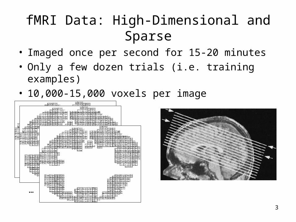
fMRI Data: High-Dimensional and Sparse

…

• Imaged once per second for 15-20 minutes• Only a few dozen trials (i.e. training examples)• 10,000-15,000 voxels per image

4

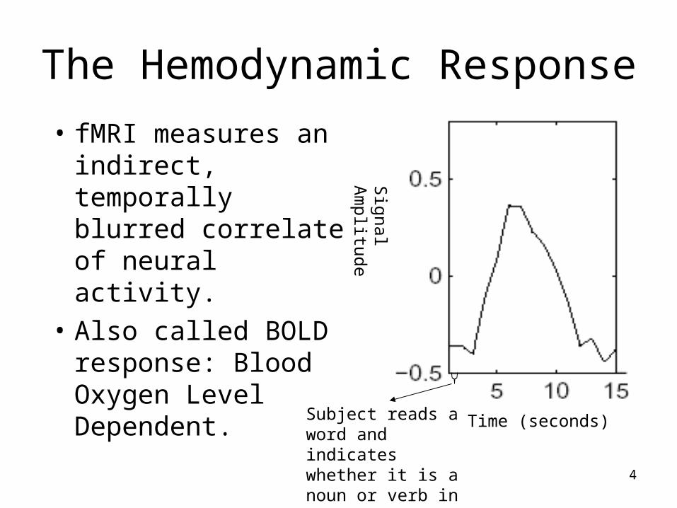
The Hemodynamic Response

Sig

nal

Am

plitu

de

Time (seconds)Subject reads aword and indicates whether it is a noun or verb in less than a second.

• fMRI measures an indirect, temporally blurred correlate of neural activity.

• Also called BOLD response: Blood Oxygen Level Dependent.

5

Study: Pictures and Sentences

• Task: Decide whether sentence describes picture correctly, indicate with button press.

• 13 normal subjects, 40 trials per subject.• Sentences and pictures describe 3 symbols: *,

+, and $, using ‘above’, ‘below’, ‘not above’, ‘not below’.

• Images are acquired every 0.5 seconds.

Read Sentence

View Picture Read Sentence

View PictureFixation

Press Button

4 sec. 8 sec.t=0

Rest

6

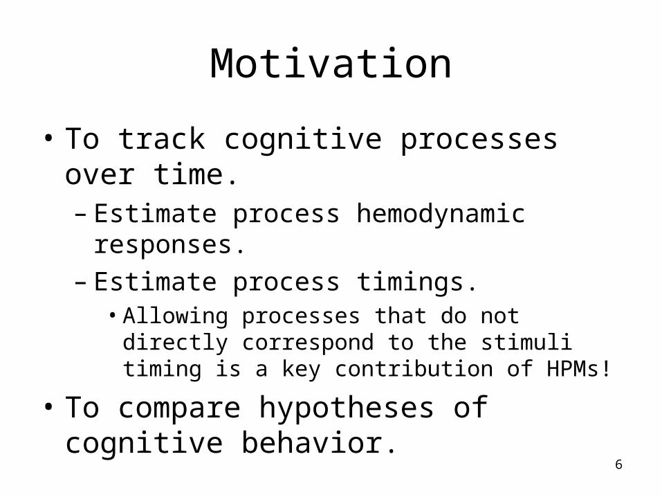
Motivation

• To track cognitive processes over time. – Estimate process hemodynamic responses.– Estimate process timings.

• Allowing processes that do not directly correspond to the stimuli timing is a key contribution of HPMs!

• To compare hypotheses of cognitive behavior.

7

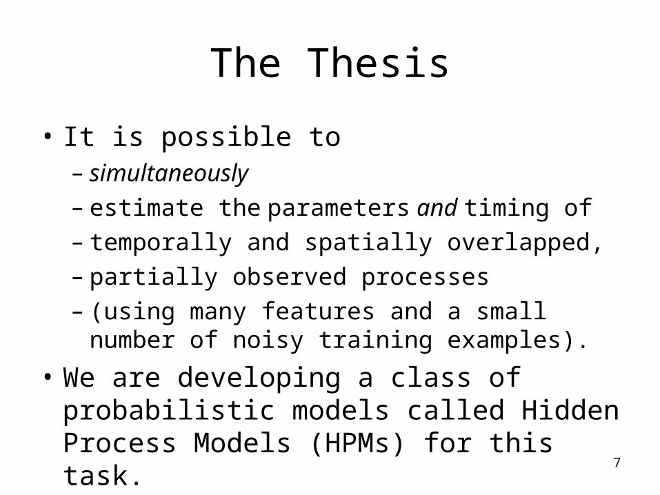
The Thesis

• It is possible to – simultaneously – estimate the parameters and timing of – temporally and spatially overlapped, – partially observed processes– (using many features and a small number of

noisy training examples).

• We are developing a class of probabilistic models called Hidden Process Models (HPMs) for this task.

8

Related Work in fMRI

• General Linear Model (GLM)– Must assume timing of process onset to

estimate hemodynamic response– Dale99

• 4-CAPS and ACT-R– Predict fMRI data rather than learning

parameters of processes from the data– Anderson04, Just99

9

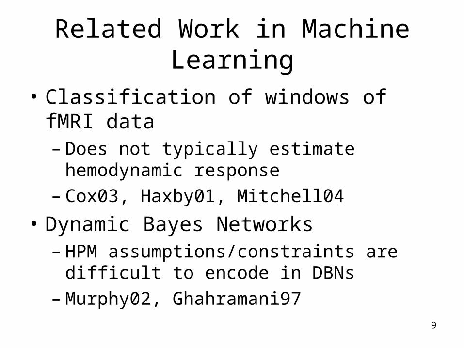
Related Work in Machine Learning

• Classification of windows of fMRI data– Does not typically estimate hemodynamic

response– Cox03, Haxby01, Mitchell04

• Dynamic Bayes Networks– HPM assumptions/constraints are difficult to

encode in DBNs– Murphy02, Ghahramani97

10

HPM Modeling Assumptions

• Model latent time series at process-level. • Process instances share parameters

based on their process types. • Use prior knowledge from experiment

design. • Sum process responses linearly.

11

HPM Formalism (Hutchinson06)

HPM = <H,C,,>H = <h1,…,hH>, a set of processes

h = <W,d,,>, a processW = response signature

d = process duration

= allowable offsets

= multinomial parameters over values in

C = <c1,…, cC>, a set of configurations

c = <1,…,L>, a set of process instances = <h,,O>, a process instance

h = process ID = associated stimulus landmark

O = offset (takes values in h)

= <1,…,C>, priors over C

= <1,…,V>, standard deviation for each voxel

Notation: parameter(entity)e.g. W(h) is the response signature of process h, and O() is the offset of process instance .

12

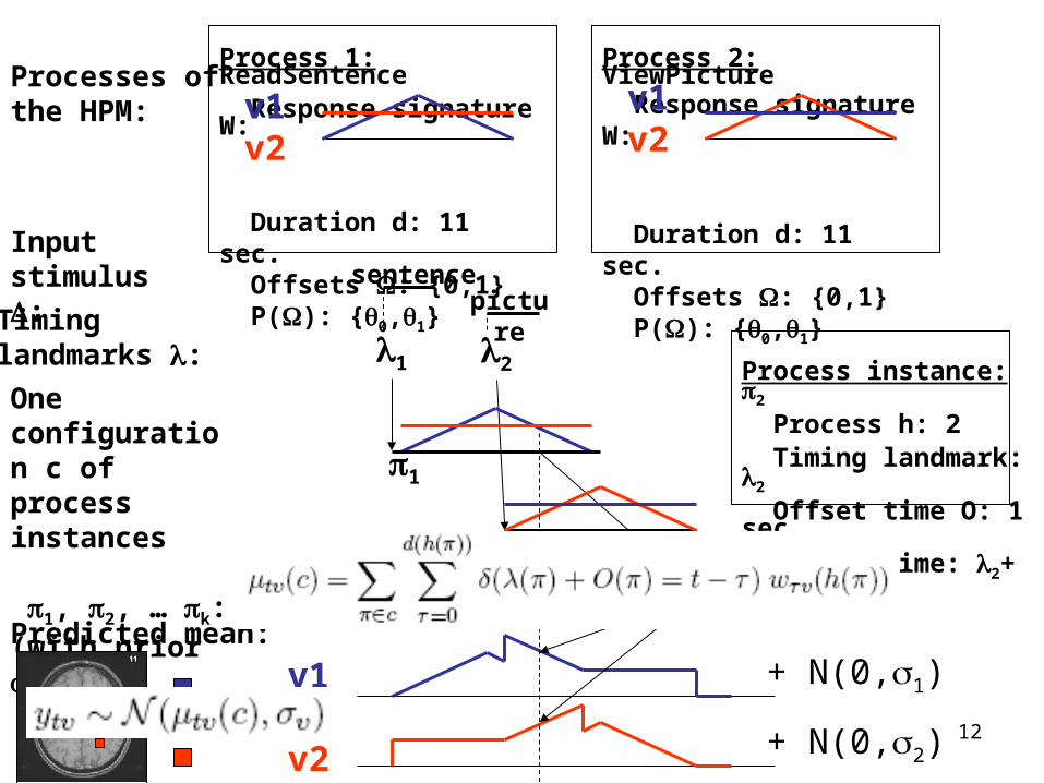
Process 1: ReadSentence Response signature W:

Duration d: 11 sec. Offsets : {0,1} P(): {0,1}

One configuration c of process instances 1, 2, … k: (with prior c)

Predicted mean:

Input stimulus :

1

Timing landmarks : 21

2

Process instance: 2 Process h: 2 Timing landmark: 2

Offset time O: 1 sec (Start time: 2+ O)

sentencepicture

v1v2

Process 2: ViewPicture Response signature W:

Duration d: 11 sec. Offsets : {0,1} P(): {0,1}

v1v2

Processes of the HPM:

v1

v2

+ N(0,1)

+ N(0,2)

13

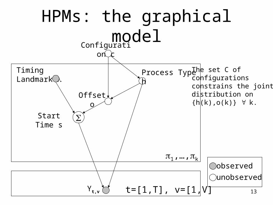
HPMs: the graphical model

Offset o

Process Type h

Start Time s

observed

unobserved

Timing Landmark

Yt,v

1,…,k

t=[1,T], v=[1,V]

The set C of configurations constrains the joint distribution on {h(k),o(k)} k.

Configuration c

14

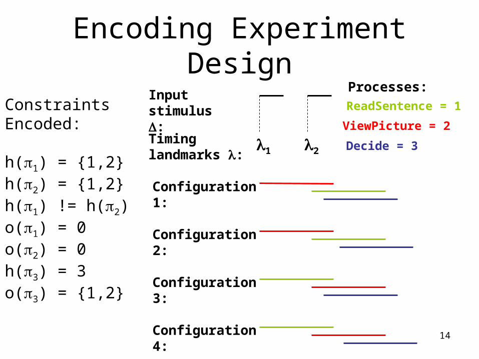
Encoding Experiment Design

Configuration 1:

Input stimulus :

Timing landmarks :

21

ViewPicture = 2

ReadSentence = 1

Decide = 3

Configuration 2:

Configuration 3:

Configuration 4:

Constraints Encoded:

h(1) = {1,2}h(2) = {1,2}h(1) != h(2)o(1) = 0o(2) = 0h(3) = 3o(3) = {1,2}

Processes:

15

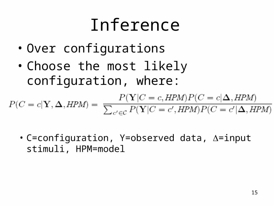
Inference• Over configurations

• Choose the most likely configuration, where:

• C=configuration, Y=observed data, =input stimuli, HPM=model

16

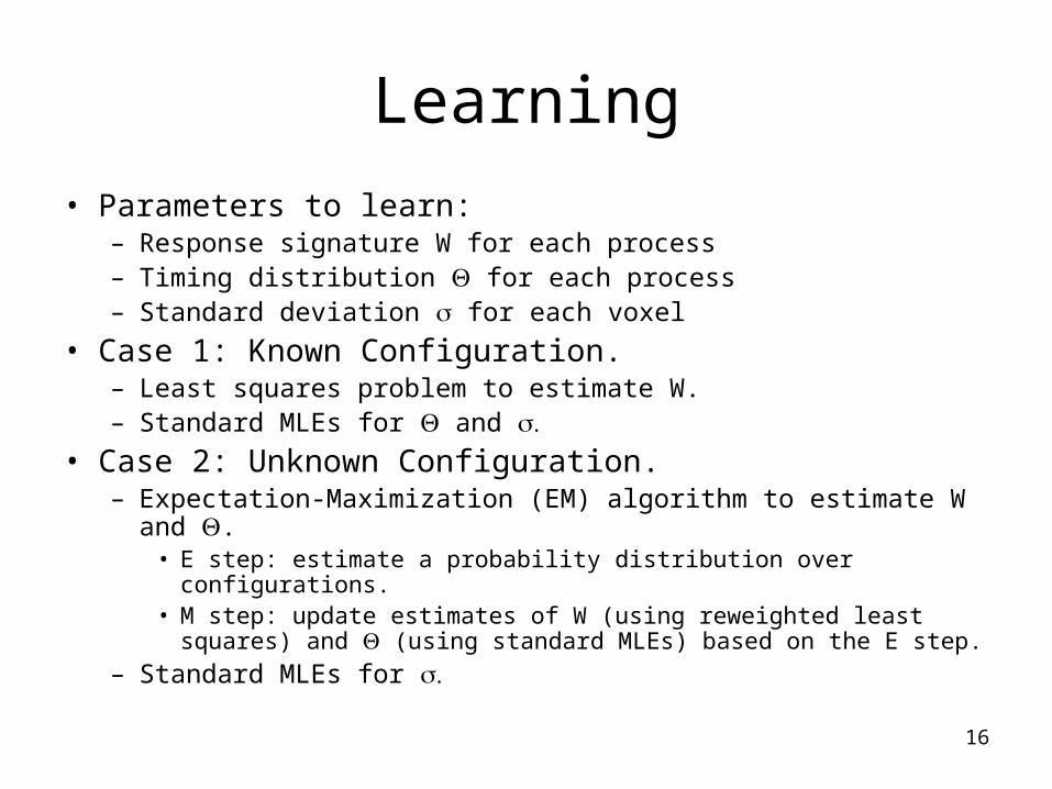
Learning

• Parameters to learn:– Response signature W for each process– Timing distribution for each process – Standard deviation for each voxel

• Case 1: Known Configuration.– Least squares problem to estimate W.– Standard MLEs for and

• Case 2: Unknown Configuration.– Expectation-Maximization (EM) algorithm to estimate W and .

• E step: estimate a probability distribution over configurations.• M step: update estimates of W (using reweighted least squares) and

(using standard MLEs) based on the E step.

– Standard MLEs for

17

Case 1: Known Configuration

• Following Dale99, use GLM.

• The (known) configuration generates a TxD convolution matrix X:

1 0 0 0 0 0 0 0 0 0 1 0 1 0 0 1 0 00 0 1 0 1 0 0 1 00 0 0 0 0 1 0 0 1… … …

d(1) d(3)

t=1t=2t=3t=4…

Configuration:1: h=1, start=12: h=2, start=23: h=3, start=2

D=hd(h)

T

d(2)

For this example, d(1)=d(2)=d(3)=3.

18

Case 1: Known Configuration

T

V

=

1 0 0 0 0 0 0 0 0 0 1 0 1 0 0 1 0 00 0 1 0 1 0 0 1 00 0 0 0 0 1 0 0 1… … …

d(1) d(3)d(2)

d(1)

d(3)

d(2)

V

W(1)

W(2)

W(3)

Y

19

Case 2: Unknown Configuration

• E step: Use the inference equation to estimate a probability distribution over the set of configurations.

• M step: Use the probabilities computed in the E-step to form weights for the least-squares procedure for estimating W.

20

Case 2: Unknown Configuration• Convolution matrix models several choices for

each time point.

1 0 0 0 0 0 0 0 0 0 0 0 1 0 0 0 0 00 1 0 0 0 0 0 0 00 0 0 0 1 0 0 0 0… … … 0 0 1 0 0 0 0 1 0 0 0 1 0 0 0 0 0 10 0 0 0 0 1 0 1 00 0 0 0 0 1 0 0 1... … …

d(1) d(3)

t=1t=1t=2t=2…t=18t=18t=18t=18…

T’>T

d(2)Configurations for each row:

3,41,23,41,2…3412…

21

Case 2: Unknown Configuration

1 0 0 0 0 0 0 0 0 0 0 0 1 0 0 0 0 00 1 0 0 0 0 0 0 00 0 0 0 1 0 0 0 0… … …

d(1) d(3)

e1e2e3e4…

d(2)

Y=

W

3,41,23,41,2…

Configurations: Weights:

e1 = P(C=3|Y,Wold,old,old) + P(C=4|Y,Wold,old,old)

• Weight each row with probabilities from E-step.

22

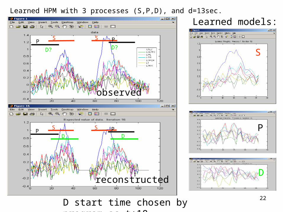
Learned HPM with 3 processes (S,P,D), and d=13sec.

P PS S

D?

observed

Learned models:

S

P

D

D start time chosen by program as t+18

reconstructed

P PS S

D D

D?

23

Results: Model Selection

• Use cross-validation to choose a model. – GNB = Gaussian Naïve Bayes– HPM-2 = HPM with ViewPicture, ReadSentence– HPM-3 = HPM-2 + Decide

Accuracy predictingpicture vs. sentence(random = 0.5)

Data log likelihood

Subject: A B C

GNB 0.725 0.750 0.750

HPM-2 0.750 0.875 0.787

HPM-3 0.775 0.875 0.812

GNB -896 -786 -476

HPM-2 -876 -751 -466

HPM-3 -864 -713 -447

24

Synthetic Data Results

• Timing of synthetic data mimics the real data, but we have ground truth.

• Can use to investigate effects of– signal to noise ratio– number of voxels– number of training examples

• on– training time– cross-validated classification accuracy– cross-validated data log-likelihood

25

26

Recall Motivation

• To track cognitive processes over time. – Estimate process hemodynamic responses.– Estimate process timings.

• Allowing processes that do not directly correspond to the stimuli timing is a key contribution of HPMs!

• To compare hypotheses of cognitive behavior.

27

Proposed Work

• Goals: – Increase efficiency.

• fewer parameters• better accuracy from fewer examples• faster inference and learning

– Handle larger, more complex problems.• more voxels• more processes• fewer assumptions

• Research areas:– Model Parameterization– Timing Constraints– Learning Under Uncertainty

28

Model Parameterization

• Goals:– Improve biological plausibility of learned responses.– Decrease the number of parameters to be estimated

(improving sample complexity).

• Tasks:– Parameter sharing across voxels– Parametric form for response signatures – Temporally smoothed response signatures

29

Timing Constraints

• Goals:– Specify experiment design domain knowledge more

efficiently.– Improve the computational and sample complexities

of the HPM algorithms.

• Tasks:– Formalize limitations in terms of fMRI experiment

design.– Improve the specification of timing constraints.– Develop more efficient exact and/or approximate

algorithms.

30

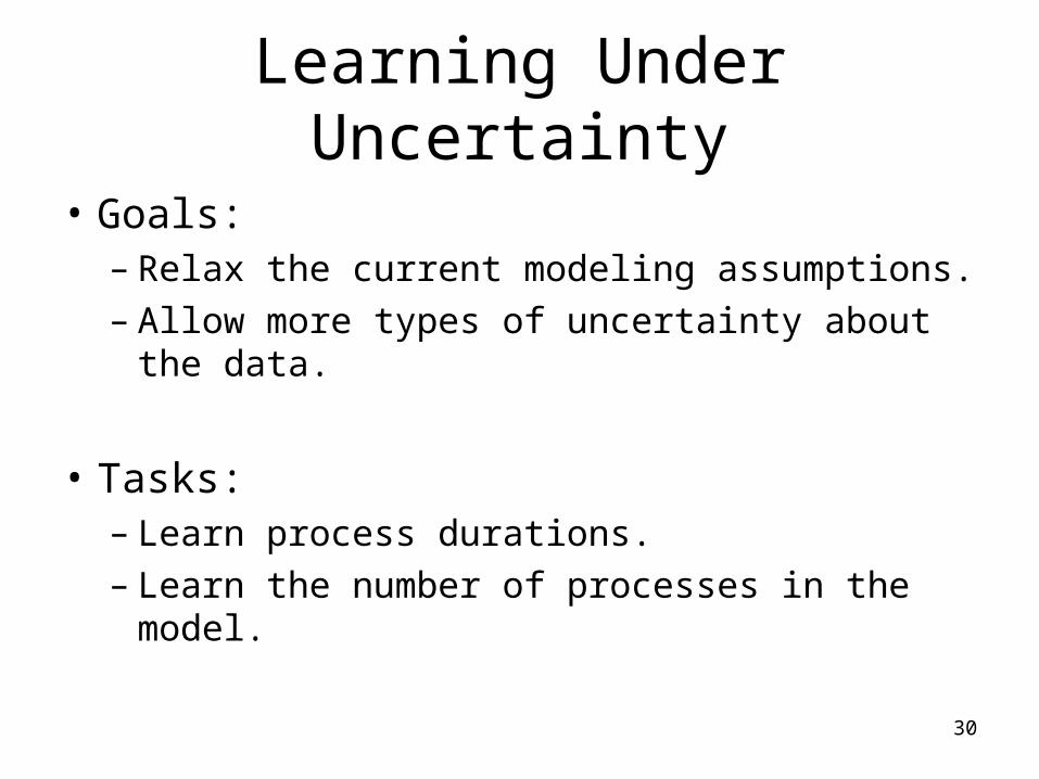
Learning Under Uncertainty

• Goals:– Relax the current modeling assumptions.– Allow more types of uncertainty about the

data.

• Tasks:– Learn process durations.– Learn the number of processes in the model.

31

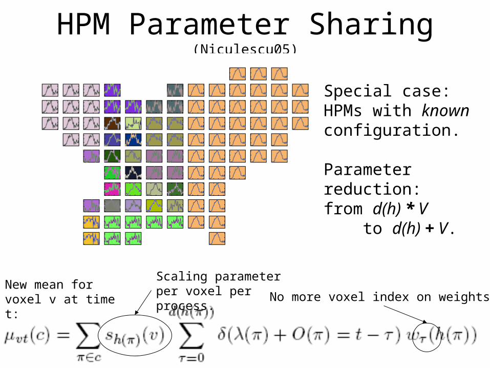
HPM Parameter Sharing (Niculescu05)

Special case: HPMs with known configuration.

Parameter reduction:from d(h) * V to d(h) + V.

Scaling parameter per voxel per process. No more voxel index on weights.

New mean for voxel v at time t:

32

Extension to Unknown Timing• Simplifying assumptions:

1. No clustering. All voxels share a response.

2. Voxels that share a response for one process share a response for all processes.

• Algorithm notes:– Residual is linear in shared response

parameters and in scaling parameters, so minimize iteratively.

– Empirically, convergence occurs within 3-5 iterations.

33

Iterative M-step: Step 1

=

W(1)

W(2)

W(3)

T’xDfor v1

T’xDfor v2

Replace ones of convolution matrix with shv. Repeat for all v.

No more voxel index here. Single column of parameters describing the shared responses.

New shape:T’V x 1

s110 0 0 0 0 0 0 0 0 0 0 s21 0 0 0 0 00 s11 0 0 0 0 0 0 00 0 0 0 s21 0 0 0 0… … …

d(1) d(3)d(2)

Ys120 0 0 0 0 0 0 0 0 0 0 s22 0 0 0 0 00 s12 0 0 0 0 0 0 00 0 0 0 s22 0 0 0 0… … …

• Using current estimates of S, re-estimate W.

34

Y =

s11 … s1V

s11 … s1V

… … …s11 .... s1V

s21 … s2V

… … …s21 ... s2V

… … …sH1 .... sHV

Each column has the scaling parameters for a voxel. The parameter for each process is replicated over its duration.

d(1)

Need to constrain these parameter sets to be equal.

Original size convolution matrix.Ones replaced with W estimates.

Iterative M-step: Step 2• Using current estimates of W, re-estimate S.

d(1) d(3)d(2)

Original size data matrix.

w110 0 0 0 0 0 0 0 0 0 0 w210 0 0 0 00 w12 0 0 0 0 0 0 00 0 0 0 w22 0 0 0 0… … …

35

Next Step?

• Implement this approach.

• Anticipated memory issues:– Replicating the convolution matrix for each

voxel in step 1. – Working on exploiting sparsity/structure of

these matrices.

• Add clustering back in

• Adapt for other parameterizations of response signatures

36

Response Signature Parameters

• Temporal smoothing

• Gamma functions

• Hemodynamic basis functions

37

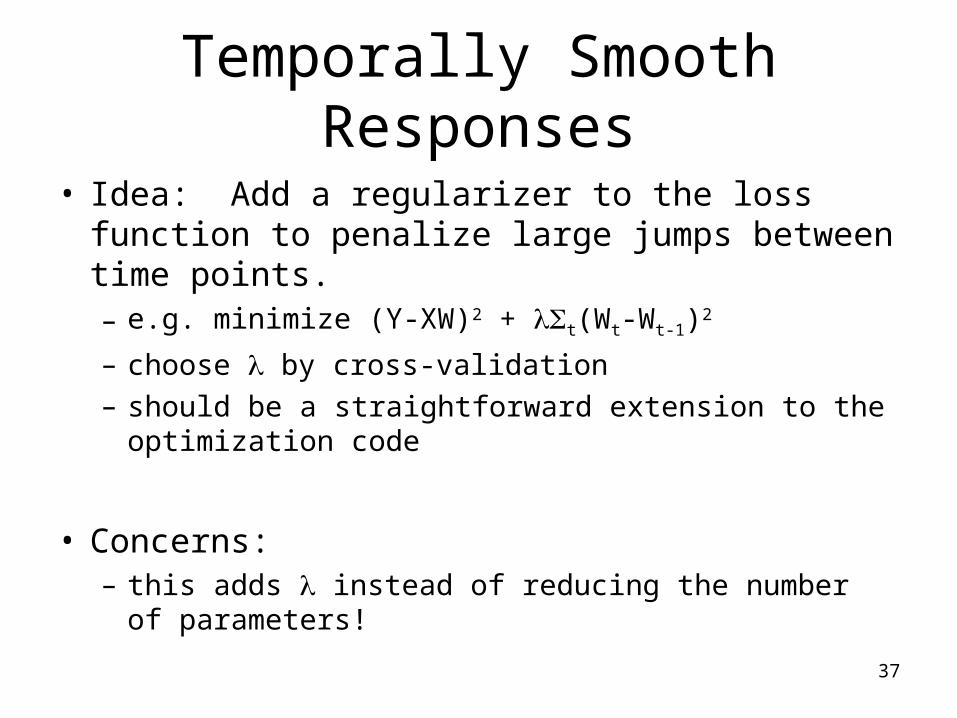
Temporally Smooth Responses

• Idea: Add a regularizer to the loss function to penalize large jumps between time points.– e.g. minimize (Y-XW)2 + t(Wt-Wt-1)2

– choose by cross-validation– should be a straightforward extension to the

optimization code

• Concerns:– this adds instead of reducing the number of

parameters!

38

Gamma-shaped Responses• Idea: Use a gamma function with 3 parameters

for each process response signature (Boynton96).

– a controls amplitude– controls width of peak– n controls delay of peak

• Questions:– Are gamma functions a reasonable modeling

assumption?– Details of how to fit parameters in M-step?

Seconds

Sig

nal A

mpl

itude

a

n

39

Hemodynamic Basis Functions

• Idea: Process response signatures are weighted sum of basis functions.– parameters are weights on n basis functions– e.g. gammas with different sets of parameters– learn process durations “for free” with variable length

basis functions– share basis functions across voxels and processes

• Questions:– How to choose/learn basis? (Dale99)

40

Schedule

• August 2006– Parameter sharing.– Progress on model parameterization.

• December 2006– Improved expression of timing constraints.– Corresponding updates to HPM algorithms.

• June 2007– Application of HPMs to an open cognitive science

problem.

• December 2007– Projected completion.

41

ReferencesJohn R. Anderson, Daniel Bothell, Michael D. Byrne, Scott Douglass, Christian Lebiere, and Yulin Qin. An integrated theory of the mind. Psychological Review, 111(4):1036–1060, 2004. http://act-r.psy.cmu.edu/about/.

Geoffrey M. Boynton, Stephen A. Engel, Gary H. Glover, and David J. Heeger. Linear systems analysis of functional magnetic resonance imaging in human V1. The Journal of Neuroscience, 16(13):4207–4221, 1996.

David D. Cox and Robert L. Savoy. Functional magnetic resonance imaging (fMRI) ”brain reading”: detecting and classifying distributed patterns of fMRI activity in human visual cortex. NeuroImage, 19:261–270, 2003.

Anders M. Dale. Optimal experimental design for event-related fMRI. Human Brain Mapping, 8:109–114, 1999.

Zoubin Ghahramani and Michael I. Jordan. Factorial hidden Markov models. Machine Learning, 29:245–275, 1997.

James V. Haxby, M. Ida Gobbini, Maura L. Furey, Alumit Ishai, Jennifer L. Schouten, and Pietro Pietrini. Distributed and overlapping representations of faces and objects in ventral temporal cortex. Science, 293:2425–2430, September 2001.

Rebecca A. Hutchinson, Tom M. Mitchell, and Indrayana Rustandi. Hidden Process Models. To appear at International Conference on Machine Learning, 2006.

Marcel Adam Just, Patricia A. Carpenter, and Sashank Varma. Computational modeling of high-level cognition and brain function. Human Brain Mapping, 8:128–136, 1999. http://www.ccbi.cmu.edu/project 10modeling4CAPS.htm.

Tom M. Mitchell et al. Learning to decode cognitive states from brain images. Machine Learning, 57:145–175, 2004.

Kevin P. Murphy. Dynamic bayesian networks. To appear in Probabilistic Graphical Models, M. Jordan, November 2002.

Radu Stefan Niculescu. Exploiting Parameter Domain Knowledge for Learning in Bayesian Networks. PhD thesis, Carnegie Mellon University, July 2005. CMU-CS-05-147.