heat balance in levitation melting: sample cooling by ... balance in levitation melting... · of...

©2015 Old City Publishing, Inc.Published by license under the OCP Science imprint,

a member of the Old City Publishing Group

High Temperatures-High Pressures, Vol. 44, pp. 429–450Reprints available directly from the publisherPhotocopying permitted by license only

429

*Corresponding author: [email protected]

Heat balance in levitation melting: Sample cooling by forced gas

convection in Helium

GeorG Lohöfer1* and Stephan Schneider

Institut für Materialphysik im Weltraum, Deutsches Zentrum für Luft- und Raumfahrt (DLR), 51170 Köln, Germany

Received: March 24, 2015. Accepted: April 14, 2015.

Electromagnetic levitation melting is a containerless processing technique for liquid metals requiring non-contact diagnostic tools. In order to prop-erly perform such experiments, a precise knowledge of the temperature-time behaviour of the metal sample resulting from the heat balance between its heating and cooling during the processing is a prerequisite. In two preceding papers we provided the necessary theoretical back-ground for the inductive heat input by the high frequency magnetic levita-tion field and the heat loss due to radiation and heat conduction through a surrounding process gas atmosphere and defined the set of experiments needed for obtaining the key parameters of the thermal model. In the pres-ent paper we extend the previous work by investigating theoretically and, at hand of further tests under microgravity, experimentally the influence of the sample cooling by forced gas convection at low Péclet number in a surrounding Helium atmosphere.

Keywords: Electromagnetic levitation, containerless processing, microgravity, gas cooling, forced convection

1 INTRODUCTION

The present work is the third one in a series of publications [1,2] investigat-ing on the basis of the energy balance between heating and cooling the temperature-time behaviour of a metal sample processed containerlessly in

430 G. Lohöfer and S. Schneider

an electromagnetic levitation facility. It is motivated by the fact, that elec-tromagnetic levitation is a widely-used, simple and robust method for the containerless, and thus mechanically and chemically unaffected, handling of hot metallic melts during the measurement of their thermophysical prop-erties or the study of their solidification behaviour [3,4].

This technique applies inhomogeneous, high frequency (≈300 kHz) electromagnetic fields, which are generated by alternating currents flowing through suitably shaped levitation coils, to induce eddy currents in a small (∅≈6 mm) metallic specimen inside the coil. Together with the original mag-netic fields these eddy currents generate a Lorentz force which levitates the metal against earth’s gravity. Furthermore, the eddy currents heat and melt the specimen due to resistive losses [3].

Performed on earth under gravity, electromagnetic levitation has, how-ever, several drawbacks. The strong magnetic force field, necessary to levitate the liquid metal against gravity

• penetratesintothematerialandgeneratesturbulentfluidflowsthatcauseunsteady disturbances (oscillations) of the droplet surface.

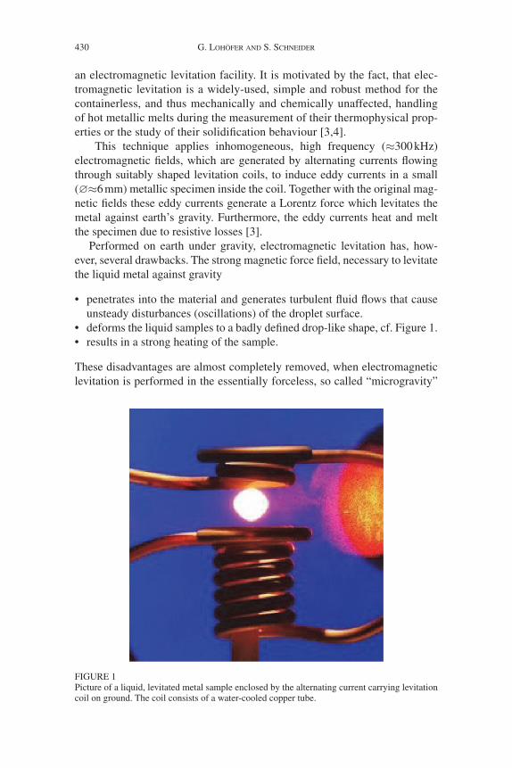
• deformstheliquidsamplestoabadlydefineddrop-likeshape,cf.Figure1.• resultsinastrongheatingofthesample.

These disadvantages are almost completely removed, when electromagnetic levitation is performed in the essentially forceless, so called “microgravity”

FIGurE 1Picture of a liquid, levitated metal sample enclosed by the alternating current carrying levitation coil on ground. The coil consists of a water-cooled copper tube.

heat BaLance in Levitation MeLtinG 431

(µg) environment, which is realised within the ≈20 seconds lasting free fall time during parabolic flights of aircrafts [5], within the ≈5 minutes lasting free fall time during sounding rocket missions or indefinitely long inside the “International Space Station” (ISS) [6]. under this condition the lifting force can strongly be reduced, and heating and positioning of the sample can be performed independently by two superposed magnetic fields [7]. Further-more, the resulting spherical shape and the absence of the gravity driven free convection of the surrounding gas atmosphere simplifies the modelling of the energy balance of the levitated sample. For all of the above mentioned carri-ers the “German Aerospace Center” (DLr) or the “European Space Agency” (ESA) provide dedicated electro magnetic levitation facilities, which are all very similar as far as the heating and cooling conditions for the levitated samples are concerned.

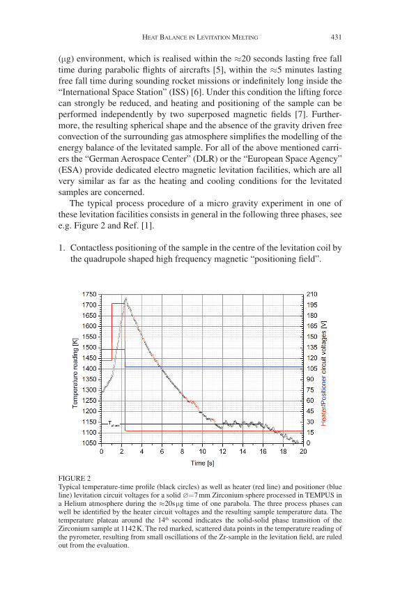
The typical process procedure of a micro gravity experiment in one of these levitation facilities consists in general in the following three phases, see e.g. Figure 2 and ref. [1].

1. Contactless positioning of the sample in the centre of the levitation coil by the quadrupole shaped high frequency magnetic “positioning field”.

FIGurE 2Typical temperature-time profile (black circles) as well as heater (red line) and positioner (blue line) levitation circuit voltages for a solid ∅=7 mm Zirconium sphere processed in TEMPuS in a Helium atmosphere during the ≈20s µg time of one parabola. The three process phases can well be identified by the heater circuit voltages and the resulting sample temperature data. The temperature plateau around the 14th second indicates the solid-solid phase transition of the Zirconium sample at 1142 K. The red marked, scattered data points in the temperature reading of the pyrometer, resulting from small oscillations of the Zr-sample in the levitation field, are ruled out from the evaluation.


2. Inductive heating and melting of the sample by the additional high fre-quency dipole shaped magnetic “heating field”.

3. Deactivation of the heating field and reduction of the positioning field, so that the liquid sample cools freely down. During this phase of minimal external impact the different experiments at the sample are performed.

In order to properly perform such an experiment procedure in these facilities, a precise prediction of the sample temperature on the basis of the heat balance between heating and cooling of the sample is a prerequisite, especially if the processing is performed fully automated and remotely.

In a preceding paper [1] we already provided the necessary theoretical background for the inductive heat input by the high frequency magnetic levi-tation fields and the heat loss due to radiation and, if carried out in a gas atmosphere, heat conduction through the surrounding gas. In a second paper [2] we extended and partly improved the previous work by detailed investiga-tions of the influence of the sample cooling by pure heat conduction in an Argon and Helium process atmosphere.

Subject of the present work is the detailed study of the heat balance of a sample under the additional influence of a forced convection cooling in a Helium gas flow. Since almost all theoretical models found in the literature to this subject deal with incompressible fluids or, if they consider compressible gases [9], are difficult to apply to practical cases, we derive in Sec. 3 a simple theoretical model on the basis of reasonable physical assumptions, and under the condition of a small Péclet number, i.e., for well conducting gases at low flow speeds. This model is then checked experimentally using a solid, spher-ical test sample of pure Zirconium (Zr) levitated in the TEMPuS parabolic flight facility during several parabolas, flown on board the “zero-g” aircraft of “Novespace” [5]. Each parabola provided a reduced (≈1/100) sample weight within a time span of ≈20 seconds. Zirconium has the advantage, that its a→b phase transition in the solid state at 1142 K is well recognizable in the pyrometrically measured temperature signal and can therefore also be used for a calibration of this signal. The micro-g environment has the additional advantage to avoid the disturbing gravity driven convection. It turns out, that our theoretical model fits very well to the experimental results found for the forced convection cooling in a Helium gas flow.

We also performed these experiments in an Argon atmosphere, where the additional influence of a forced Argon gas flow on the sample cooling has been measured. However, due to the low thermal conductivity of Argon com-pared to that of Helium, the requirement of a small Péclet number is violated and our theoretical model fails in this case. Thus, we will leave the presenta-tion of the Argon results and the derivation of a suitable theoretical descrip-tion to a later publication.

Although the resulting thermal model is adapted to the TEMPuS and the other µg electromagnetic levitation facilities, it is of sufficient generality to be


transferred also to any ground based electromagnetic levitation facility. In this case, however, also gravity driven natural convection cooling of the sam-ple by the surrounding process gas atmosphere has to be taken into account.

2 EXPERIMENTAL SITUATION

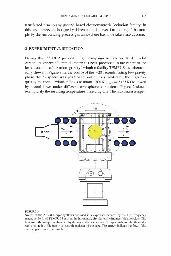
During the 25th DLr parabolic flight campaign in October 2014 a solid Zirconium sphere of 7 mm diameter has been processed in the centre of the levitation coils of the micro gravity levitation facility TEMPuS, as schemati-cally shown in Figure 3. In the course of the ≈20 seconds lasting low gravity phase the Zr sphere was positioned and quickly heated by the high fre-quency magnetic levitation fields to about 1700 K (Tmelt = 2125 K) followed by a cool-down under different atmospheric conditions. Figure 2 shows exemplarily the resulting temperature-time diagram. The maximum temper-

FIGurE 3Sketch of the Zr test sample (yellow) enclosed in a cage and levitated by the high frequency magnetic fields of TEMPuS between the horizontal, circular coil windings (black circles). The heat from the sample is absorbed by the internally water cooled copper coils and the thermally well conducting silicon nitride ceramic pedestal of the cage. The arrows indicate the flow of the cooling gas around the sample.


ature of 1700 K was still low enough for the sample to cool in a surrounding Helium atmosphere to its solid phase transition temperature at 1142 K, which is used as calibration point for the contactless pyrometric tempera-ture measurement.

During the 5 flown parabolas, the following 5 different cooling conditions for the solid, spherical Zr test sample have been set:

1st Parabola: Cooling in a static Helium gas atmosphere.2nd–5th Parabola: Cooling in the Helium atmosphere with an additional gas

flow, driven by a circulation pump at motor voltages of 5V, 9V, 13V and 16.9V, respectively.

• DuringallexperimentcyclesthepressureoftheHeliumatmospheresur-rounding the sample was 350 ± 2 mbar.

• Duringallcoolingcyclesthevoltagegeneratingthemagneticpositioningfield has constantly been set to 108V and the voltage generating the mag-netic heating field to 18V, so that the induced power from the magnetic levitation fields was always the same.

• Duetotheweightlessnessduringthesamplecoolingphasegravitydrivennatural convection cooling in the surrounding gas could be neglected.

The detailed properties of the solid Zirconium test sphere were [8]:

• Meltingtemperature:TM = 2125 K.• Solidphasetransitiontemperature:Tphase = 1142 K.• Meanspecificheatinthesolidbetween1200 K < T < 1600 K: cp = 0.334

[Ws/(gK)].• Samplemass:m = 1.17 g.• Sampleradius:a = 3.50 mm.

3 PHYSICAL BASICS

The basis for the temperature behaviour of the sample inside the TEMPuS facility is provided by the heat balance equation, the detailed derivation of which is described in [1].

dE t

dtm c

dT t

dtP t P T t P T t Pp

ind radgascon

gasfl( ) ( )

( ) ( ( )) ( ( ))= = − − − oow T t( ( )) (1)

The internal energy change dE / dt of the levitated material results in a time dependent temperature change dT / dt depending on the temperature T, the mass m, and the specific heat cp of the spherical isothermal sample. The con-sidered external power in- and output is due to


• Pind, which denotes the inductive heat transfer from both high frequency electromagnetic levitation fields of TEMPuS to the sample. Pind was the same during all cooling phases.

• Prad (T), which denotes the temperature dependent radiative heat transfer between the sample and its environment (sample holder, vacuum container, coil). Since the sample surface and the environment remained always the same, this function did not change during all cooling phases.

• P Tgascon ( ), which denotes the temperature dependent heat transfer between

the sample and its environment (sample holder, vacuum container, coil) solely by heat conduction through the static surrounding gas atmo-sphere. Since for the same atmosphere the environment remained always the same, this function did not change during the corresponding cooling cycles.

• P Tgasflow ( ), which denotes the temperature dependent heat transfer between

the sample and its environment (sample holder, vacuum container, coil) solely by forced convection in the surrounding gas atmosphere.

Whereas the functions Pind, Prad (T) and P Tgascon ( ), where the indices “gas” or

“g” stand here for “He” or “Ar”, have already been investigated in [1] and [2], the function P THe

flow ( ) will be investigated in detail in the present work. To keep the calculations via Eq. (1) and the determination of the material spe-cific quantities from measured temperature-time diagrams manageable, it will be assumed, that:

• All samplematerial specificquantitiesareconsidered tobe temperatureindependent.

3.1 Heat conduction cooling modelFor pure heat conduction in an Argon or Helium gas a model for the tempera-ture dependence of the sample power loss has already been derived in [1] and [2]

P Ta

a bT dT

a

a bTgas

con

gg g g

K

T

g

g

g

g( ) ( ) ,=−

=− +

⋅ −∫ +4

1

4

1 1300

0 1πλ

π λ

αα (( )300 1

K gα +( ), (2)

where the pressure independent kinetic model for the thermal conductivity of a gas

λ λ αg g g gT T g( ) ,= ⋅0 , (3)

has been used. Here T denotes the temperature of the isothermal sample and Tg that of the particular gas. The coefficients ag and l0,g and bg for Argon and Helium gas are listed in Table 1.


Equation (2), which describes the real situation in TEMPuS relatively well, has been derived under the simplifying assumption of a radially symmetric heat flow through the gas from the spherical sample of temperature T and radius a to a radially symmetric heat sink of 300 K a distance bg away from the sample centre, see the dashed lines in Figure 3.

3.2 Forced gas flow cooling modelConvective gas cooling means, that heat from the hot sample is not only transported by diffusion (conduction) through the gas to the cold heat sink but also by a superposed movement of the gas. Analogue to the calculations of the pure heat conduction in [1] the general equations, relevant for this extended situation are the heat conservation equation [10, Sec. 3.2]

ρg p g g g gcont c

d

dtT t

d

dtp t t( , ) ( , ) ( , ) ( , ),x x x j x− = −∇⋅ , (4)

where under consideration of Eq. (3)

j x x x xgcon

g g gg

g

t T t T t T tg

g( , ) : ( ( , )) ( , ) ( , ),= − ∇ = −+

∇ +λλ

αα0 1

1 (5)

describes the heat flow density by conduction in the gas, and the mass conser-vation equation

∂∂

+∇⋅( ) =t

t t tg gρ ρ( , ) ( , ) ( , )x v x x 0 . (6)

In these equations ρg(x, t), ρg(x, t), and v(x, t) denote the mass density, the pressure and the velocity field of the moving gas, respectively, and cp,g its specific heat (related to the mass) at constant pressure. The above equations are simplified by the following considerations:

1. In Eq. (4) a possible heat generation in the gas by the viscous shear flow, which is however much smaller than the heat input from the hot sample, has already been neglected.

2. Helium and Argon, which we use for cooling, can be considered as one-atomic ideal gases, satisfying the ideal gas law

TAbLE 1Heat conduction coefficients for He- and Ar-gas

gas ag λ0,g[W /(m · Kag + 1)] bg [mm]

He 0.7 2.86 10-3 14.4

Ar 0.7 3.39 10-4 9.55


p t RT t t mg g g mol( , ) ( , ) ( , ) /x x x= ρ and the relation c m Rp g mol, /= 5 2

where mmol denotes the molar mass of the gas and R the universal gas con-stant.

3. As long as the flow of the cooling gas around the spherical sample remains laminar and below a speed of ≈50 m/s, the pressure in the gas may consid-ered to be constant, i.e., p t pg ( , )x = ∞. This follows from the fact, that the maximum pressure in the flow occurs at the stagnation point in front of the object, where (for an inviscid gas) [11]

p p v pm v

RTp

s

mgmol

,max //

= + = +

< +∞ ∞ ∞ ∞∞

∞∞

−ρ 22

52

2 12

1 1022

2

∞v

Here p∞, ρ∞, T K∞ = 300 and v∞ are the constant values of pressure, den-sity, temperature and uniform flow speed of the gas far from the sphere.

4. Due to an estimation performed in [1], showing that the temperature equilibration in the gas proceeds much quicker than the temperature change of the sample, only the steady parts of both balance equations (4) and (6) need to be considered, i.e., terms containing the partial time deriv-ative ∂ ∂t (also in d dt t/ /≡ ∂ ∂ + ⋅∇v ) may be disregarded.

Taking these results into account, the heat balance equation (4) assumes the steady form

∇⋅ +

=j x j xg

congflow( ) ( ) 0, (7)

where

j x v xgflow p( ) : / ( )= ∞5 2 (8)

can be interpreted as convective heat flow density, and the mass balance equa-tion (6) now reads

∇⋅

=v x x( ) / ( )Tg 0. (9)

Volume integration of Eq. (7) over a spherical shell S(r) inside the gas, which is bordered at its inside by the spherical sample and at is outside by a spheri-cal surface of radius r, see Figure 4, yields

sample spherical outersurface boundary of S(r)

spherical outerboundary of S(r)

0 ( ) ( ) ( ) ( ) ( ) ( ) ( ) ( )

5( ( )) ( ) ( ) ( ) ( ) (2

con flow con flowsample g g g g

gas g g g

dS dS

P T T dS p dSr

λ ∞

= − ⋅ + + ⋅ +

∂= − + − + ⋅

∂

∫ ∫

∫

n x j x j x x n x j x j x x

x x x n x v xspherical outerboundary of S(r)

)∫ x. (10)


Here the Gauss’s integral theorem has been used, and n as well as nsample denote the radial outwardly directed normal vectors on the corresponding surfaces. The above result considers, that the normal component of the gas flow on the sample surface disappears n vsample ⋅ = 0 , and that the

integral n jsample gcon dS⋅∫sample

surface

over the sample surface corresponds to the

total heat flow (power) Pgas from the sample into the gas.To obtain the real velocity field v(x) of the cooling gas flowing around the

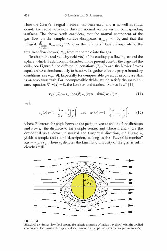
sphere, which is additionally disturbed in the present case by the cage and the coils, see Figure 3, the differential equations (7), (9) and the Navier-Stokes equation have simultaneously to be solved together with the proper boundary conditions, see e.g. [9]. Especially for compressible gases, as in our case, this is an ambitious task. For incompressible fluids, which satisfy the mass bal-ance equation ∇⋅ =v x( ) 0, the laminar, undisturbed “Stokes flow” [11]

v nSt nr v w r w r( , ) : cos( ) ( ) sin( ) ( )θ θ θ τ= −[ ]∞ τ (11)

with

w ra

r

a

rn ( ) := − +

1

3

2

1

2

3

and w ra

r

a

rτ ( ) := − −

1

3

4

1

4

3

, (12)

where q denotes the angle between the position vector and the flow direction and r : | |= x the distance to the sample centre, and where n and τ are the orthogonal unit vectors in normal and tangential direction, see Figure 4, yields a simple and sound description, as long as the “reynolds number” Re : /= ∞v a gν , where vg denotes the kinematic viscosity of the gas, is suffi-ciently small.

FIGurE 4Sketch of the Stokes flow field around the spherical sample of radius a (yellow) with the applied coordinates. The crosshatched spherical shell around the sample indicates the integration area S(r).


To approximate the Stokes flow to our situation of a compressible gas, where the mass balance equation (9) holds, we suppose tentatively

v x v x x( ) ( ) ( )= ∞St gT T , (13)

so that v(x) now satisfies Eq. (9) and approaches the Stokes flow away from the sample where T T Kg ( )x ≈ =∞ 300 . We leave it to the experimental check in Sec. 4 to judge, whether this simple modification, which does not consider the Navier-Stokes equation, is acceptable or not.

3.2.1 Forced convection at low Péclet numberIn deriving the power loss for the pure heat conduction (| ( ) |v x = 0) in [1], which resulted in Eq. (2), a spherically symmetric temperature distribution T T rg g( ) ( )x = in the gas around the sample has been assumed for simplicity, i.e., a dependence on the radial coordinate r : | |= x only. Consequently, also the heat sink of the resulting purely radial heat flow far away from the sample, where the gas is cooled down to the ambient temperature T K∞ = 300 , has to consist in this case of a spherical surface of radius bg, see Sec. 3.1, which means that

T b Tg g( ) = ∞. (14)

regardless of the complicated, non-spherical geometry of the heat sinks near the sample (coil, cage pedestal, vacuum chamber), see Figure 3, Eq. (2) describes the real situation pretty well, as can be seen from the experimental results found in [2]. under these conditions Eq. (10) immediately results for r = bg in

P P b T bT r

rgas gascon

g g g gg

r bg

= = −∂

∂=

: ( ( ))( )

4 2π λ

. (15)

If the gas additionally moves with a velocity | ( ) |v x ≠ 0, as visualised in Figure 4, this simple spherically symmetric temperature distribution T rg ( ) of the gas does no longer hold and the real temperature field has in general to be calculated from the partial differential equations (7) and (9) together with the Navier-Stokes equation for the compressible flow field. If however the con-vective heat flow, defined in Eq. (8), is small compared to the conductive one, defined in Eq. (5), which means that the relation between both, characterized by the dimensionless local Péclet number, satisfies

j x

j xx

v x

x x

gflow

gcon

g g g

Pep

T T

( )

( )( ) :

( )

( ( )) ( )≈ =

∇<<∞5

21

λ, (16)


it is reasonable to assume, that the resulting temperature distribution Tg (x) in the gas consists of the original spherical temperature distribution T rg ( ), how-ever, locally shifted in flow direction v x v x( )/ | ( ) | proportional to a small dis-tance of the order of a Pe(x), where the sample radius a is considered to be the typical length scale in the system

T T C a Pe T r C a Peg g g( ) ( )( )

| ( ) |( ) ( )

(x x x

v xv x

xv x

≈ −

≈ −

))

| ( ) |( )

( )( ) ( )

( ( )) (

v xx v x n

x

⋅∇

= −⋅

∇∞

∞

T r

T r CT

T

a p

T T

g

gg St

g g g

5

2 λ xx)

( )

( )( )

( ( ))cos( )

∂

∂

≈ +

∞ ∞

∞

T r

r

T r Ca p v w r

T r T

g

gn

g g

15

2 λθ

. (17)

Above, the shifted � …Tg ( ) was expanded around each point x in the space up to the linear order in Pe(x), and the Eqs. (16), (13) and (11) were inserted. Furthermore, since according to Eq. (17) T T r O Peg g( ) ( ) ( )x = +( ) 1 , and since terms of higher order than O(Pe) should be neglected, Tg(x) on the right hand side of (17) could everywhere be replaced by T rg ( ). The a priory unknown constant of proportionality C > 0 in Eq. (17) is assumed to be of O(1) and must be determined experimentally by a fit to measurement values.

under consideration of the Eqs. (3) and (15) and with the above result for Tg(x) the first integral of Eq. (10) then results for r = bg in

−∂∂

=−

∫ λλ

g g gTr

T dS( ( )) ( ) ( )x x xspherical outerboundary of S(b )g

0,, ( ) ( )g

ggr

T dSg

α

λ

α

+∂∂

=−

+∫11 x x

spherical outerboundary of S(b )g

00 2 1 1

01

2 1, ( ) ( ( )) cos sing

gg gb

rT r O Pe r dg g

απ θ θ θα α

π

+∂∂

+( )

+ +

∫

≈ −∂

∂=

=

=

r b

g g g gg

r b

gascon

g

g

b T bT r

rP T4 2π λ ( ( ))

( )( )

, (18)

after Taylor’s theorem has been applied to the integrand and terms of higher order than O(Pe) have been neglected. With the Eqs. (13), (11), (17) and (14) the third term of Eq. (10) yields for r = bg

5

2

5

2p dS

p v

T∞∞ ∞⋅ =∫ n x v x x( ) ( ) ( )

spherical outerboundary of S(b )g

∞∞ =

∞ ∞

∫

≈

w r r T d

C ba p v

n g

r b

g

g

( ) ( ) cos sin2

25

3

2

0

22

π θ θ θ

π

π

x

22 2w b

Tn g

g

( )

( )λ ∞

, (19)


after terms of higher order than O(Pe) have been neglected. With these results Eq. (10) finally yields

P T P T Pgas gascon

gasflow( ) ( )= + . (20)

In Eq. (20) P Tgascon ( ) just corresponds to the sample power loss by pure heat

conduction through a static gas atmosphere, already provided by Eq. (2), and

P C a b a b p vgasflow

g g g: / /= −( ) ∞ ∞1 3 2 2 , (21)

where in our case due to ( / ) .a bg2 0 07< only terms of O a bg( / ) in w bn g

2 ( ) have been considered, describes the sample power loss by the additional movement of the gas. The constant Cg > 0 in Eq. (21) combining bg, λ0,g, and ag is purely gas type and facility specific and can be determined experi-mentally by a fit to measured values. It is remarkable that Pgas

flow does not depend on the sample temperature T.

As we will see below by a check with experimental data, Eq. (20), com-posed of Eq. (2) and (21), yields a good description of the thermal power loss from the sample by forced convection in the thermally very well conducting Helium gas. For the poorly conducting Argon gas however, where according to Table 1 λ λAr He≈ 0 1. , this equation fails, because the condition of Eq. (16) is no longer satisfied. Here, we only note this result for the Argon gas and leave its presentation to a later publication. Therefore, in this section all indi-ces “gas” or “g” represent “He” only.

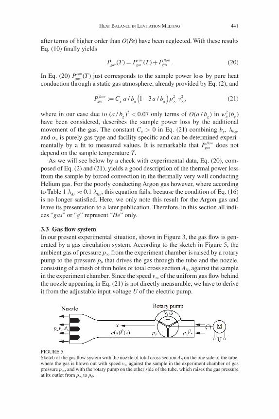
3.3 Gas flow systemIn our present experimental situation, shown in Figure 3, the gas flow is gen-erated by a gas circulation system. According to the sketch in Figure 5, the ambient gas of pressure p∞ from the experiment chamber is raised by a rotary pump to the pressure pp that drives the gas through the tube and the nozzle, consisting of a mesh of thin holes of total cross section AN, against the sample in the experiment chamber. Since the speed v∞ of the uniform gas flow behind the nozzle appearing in Eq. (21) is not directly measurable, we have to derive it from the adjustable input voltage U of the electric pump.

FIGurE 5Sketch of the gas flow system with the nozzle of total cross section AN on the one side of the tube, where the gas is blown out with speed v∞ against the sample in the experiment chamber of gas pressure p∞, and with the rotary pump on the other side of the tube, which raises the gas pressure at its outlet from p∞ to pP.


The power unit of the pump consists of a direct-current motor. According to [12, Chap. 13], its input voltage U is linearly related to its rotational fre-quency n

. and its torque M via U c n c Mm m= +1 2 , where cm1 and cm2 are two

positive, motor specific constants. Neglecting small frictional forces, the torque M, exerted on the motor from the pumping unit, is essentially propor-tional to the forces applied on the vanes of the pump, which result from the pressure difference between its outlet and inlet, i.e., M p pP∝ − ∞. On the other hand the volume flow V

.P into the pumping unit at its inlet just corre-

sponds to the pump specific volume VP which per turn is shoved through the pump, see Figure 5, times its rotational frequency n

. , i.e., V V nP P= ⋅ . Thus,

the relation between the accessible motor input voltage and the conditions in the gas flow system now reads

U c V c p pP P= + − ∞1 2 ( ) (22)

where c1 and c2 are two positive constants, specific of the pumping unit. A relation between the conditions at the nozzle exit and in the tube is pro-

vided by the stationary form of the mass conservation equation (6). Taking the ideal gas law under the assumption of isothermal conditions in the tube into account, it reads ∇⋅[ ]=v x x( ) ( )p 0. Volume integration of this equation over the tube from the nozzle exit to any point x in the tube, thereby using the Gauss integral theorem, results in

p v A p x v x A x p x V x p VN P∞ ∞ ∞= ≡ =( ) ( ) ( ) ( ) ( ) , (23)

where v(x) as well as v∞ represent the respective mean gas speeds at the point x in the tube and behind the nozzle, averaged over the corresponding cross sections A(x) and AN. The quantity V x v x A x( ) : ( ) ( )= defines the mean volume flow at the point x in the tube.

To obtain the unknown pressure pp at the pump outlet, the local Hagen-Poiseuille law [11]

V xR x dp x

dxg

( )( ) ( )

= −πη

4

8

is used. It relates the volume flow of a fluid of viscosity ηg at any point x in a circular tube of radius R(x) to the local pressure drop. Elimination of V

.(x) by

Eq. (23) and integration of the resulting differential equation along the flow direction from the pump outlet at pressure pp to the nozzle exit at pressure p∞ yields

p p c v pP g= +∞ ∞ ∞1 3η , (24)


where c3 is a positive, flow system specific constant. The solution of the qua-dratic equation for v∞, resulting from the insertion of the Eqs. (23) and (24) into Eq. (22), finally yields

v c cU p cc

c

cU

pgg

g

∞ ∞ ∞∞

= + +( ) − ++( )

1 1 12

12

, (25)

where p p∞ ∞=: / 350 mbar defines the normalized ambient pressure. The positive, gas type specific constant cg g∝ η as well as the two positive flow system specific constants c∞ and c have to be determined by a fit to experi-mental values.

For large and small pump voltages U, where Eq. (25) behaves as v c cU

U∞ →∞ ∞ → and v c c c c UU g g∞ → ∞ → − +

01 1[ / ( )] , respectively, it

becomes immediately evident, that the two constants c∞ and c are strongly correlated. Therefore, without significantly changing the functional behav-iour of (25), c can arbitrarily be set to c V= −1 1[ ], so that the relation between v∞ and U now reads

v c U p cc

c

U

pgg

g

∞ ∞ ∞∞

≈ + +( ) − ++( )

1 1 12

12

, (26)

with the normalized pump voltage U U V: / [ ]= 1 , and with only the two con-stants c∞ and cg that have to be determined by a fit to experimental values.

4 EXPERIMENTAL RESULTS

To obtain experimentally the sample power loss in the case, that the sample in the gas atmosphere is subjected to an additional forced gas flow, we apply Eq. (1) on the cooling ranges of the temperature-time diagrams measured for the Zr test sample during the parabolas No. 2 – No. 5, see Sec. 2

m cdT t

dtP P T P T P Tp

gas flow

ind radgascon

gasflow( )

( ) ( ) ( )−

= − − − . (27)

The sum of the induced electrical power input term Pind, the radiation power loss function Prad (T) and the heat conduction power loss function in the gas P Tgas

con ( ) on the right hand side of Eq. (27), can be obtained, if Eq. (27) is applied on the cooling range of the temperature-time diagram measured for the Zr test sample during parabola No. 1, where P Tgas

flow ( ) = 0, see Sec. 2

m cdT t

dtP P T P Tp

gas stat

ind radgascon( )

( ) ( )−

= − − .


Then the measured power loss, solely by the convective gas flow, results for our Zr test sample in

P TWs

K

dT

dtT

dT

dtTgas

flow

gas stat gas flo

( ) . ( ) ( )=

−− −

0 391ww

(28)

where its value of mcp has be inserted. This measured temperature dependent

power loss function P Tgasflow ( ) will then be compared with the physical model

equation (21) and (26) for Helium to check its applicability and to obtain the unknown constants of the model.

4.1 Sample cooling in Helium

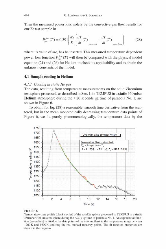
4.1.1 Cooling in static He gasThe data, resulting from temperature measurements on the solid Zirconium test sphere processed, as described in Sec. 1, in TEMPuS in a static 350 mbar Helium atmosphere during the ≈20 seconds µg time of parabola No. 1, are shown in Figure 6.

To obtain for Eq. (28) a reasonable, smooth time derivative from the scat-tered, but in the mean monotonically decreasing temperature data points of Figure 6, we fit, purely phenomenologically, the temperature data by the

FIGurE 6Temperature-time profile (black circles) of the solid Zr sphere processed in TEMPuS in a static 350 mbar Helium atmosphere during the ≈20 s µg time of parabola No. 1. An exponential func-tion (green line) is fitted to the data points of the cooling flank in the temperature range between 1200 K and 1600 K omitting the red marked runaway points. The fit function properties are shown in the diagram.


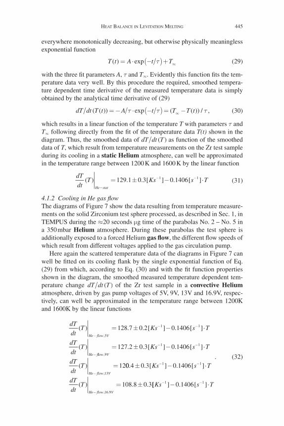
everywhere monotonically decreasing, but otherwise physically meaningless exponential function

T t A t T( ) exp= ⋅ −( )+ ∞τ (29)

with the three fit parameters A, t and T∞. Evidently this function fits the tem-perature data very well. by this procedure the required, smoothed tempera-ture dependent time derivative of the measured temperature data is simply obtained by the analytical time derivative of (29)

dT dt T t A t T T t( ( )) exp ( ( )) /= − ⋅ −( ) = −∞τ τ τ , (30)

which results in a linear function of the temperature T with parameters t and T∞ following directly from the fit of the temperature data T(t) shown in the diagram. Thus, the smoothed data of dT dt T( ) as function of the smoothed data of T, which result from temperature measurements on the Zr test sample during its cooling in a static Helium atmosphere, can well be approximated in the temperature range between 1200 K and 1600 K by the linear function

dT

dtT Ks s T

He stat

( ) [ ] . [ ]−

− −= ± − ⋅129.1 0.3 1 10 1406 (31)

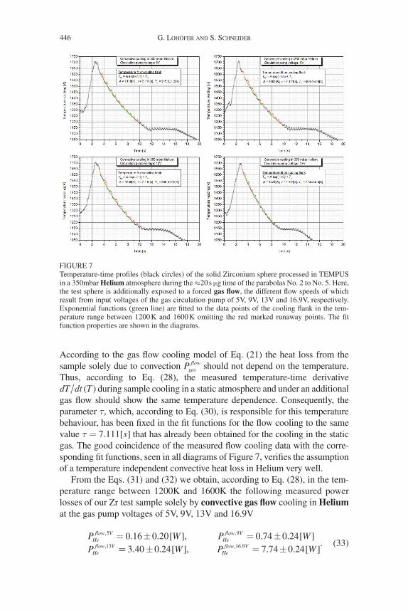
4.1.2 Cooling in He gas flowThe diagrams of Figure 7 show the data resulting from temperature measure-ments on the solid Zirconium test sphere processed, as described in Sec. 1, in TEMPuS during the ≈20 seconds µg time of the parabolas No. 2 – No. 5 in a 350 mbar Helium atmosphere. During these parabolas the test sphere is additionally exposed to a forced Helium gas flow, the different flow speeds of which result from different voltages applied to the gas circulation pump.

Here again the scattered temperature data of the diagrams in Figure 7 can well be fitted on its cooling flank by the single exponential function of Eq. (29) from which, according to Eq. (30) and with the fit function properties shown in the diagram, the smoothed measured temperature dependent tem-perature change dT dt T( ) of the Zr test sample in a convective Helium atmosphere, driven by gas pump voltages of 5V, 9V, 13V and 16.9V, respec-tively, can well be approximated in the temperature range between 1200K and 1600K by the linear functions

dT

dtT Ks s T

dT

dtT

He flow V

He f

( ) [ ] . [ ]

( )

,−

− −

−

= ± − ⋅5

1 10 1406128.7 0.2

llow V

He flow V

Ks s T

dT

dtT

,

,

[ ] . [ ]

( )

9

1 1

13

0 1406= ± − ⋅

=

− −

−

127.2 0.3

1200.4 0.3

108.8 0.3

± − ⋅

= ±

− −

−

[ ] . [ ]

( ), .

Ks s T

dT

dtT

He flow V

1 1

16 9

0 1406

[[ ] . [ ]Ks s T− −− ⋅1 10 1406

. (32)


FIGurE 7Temperature-time profiles (black circles) of the solid Zirconium sphere processed in TEMPuS in a 350mbar Helium atmosphere during the ≈20 s µg time of the parabolas No. 2 to No. 5. Here, the test sphere is additionally exposed to a forced gas flow, the different flow speeds of which result from input voltages of the gas circulation pump of 5V, 9V, 13V and 16.9V, respectively. Exponential functions (green line) are fitted to the data points of the cooling flank in the tem-perature range between 1200 K and 1600 K omitting the red marked runaway points. The fit function properties are shown in the diagrams.

According to the gas flow cooling model of Eq. (21) the heat loss from the sample solely due to convection Pgas

flow should not depend on the temperature. Thus, according to Eq. (28), the measured temperature-time derivative dT dt T( ) during sample cooling in a static atmosphere and under an additional gas flow should show the same temperature dependence. Consequently, the parameter t, which, according to Eq. (30), is responsible for this temperature behaviour, has been fixed in the fit functions for the flow cooling to the same value τ = 7 111. [ ]s that has already been obtained for the cooling in the static gas. The good coincidence of the measured flow cooling data with the corre-sponding fit functions, seen in all diagrams of Figure 7, verifies the assumption of a temperature independent convective heat loss in Helium very well.

From the Eqs. (31) and (32) we obtain, according to Eq. (28), in the tem-perature range between 1200K and 1600K the following measured power losses of our Zr test sample solely by convective gas flow cooling in Helium at the gas pump voltages of 5V, 9V, 13V and 16.9V

P W P WP

Heflow V

Heflow V

Heflow V

, ,

,

. . [ ], . . [ ]5 9

13

0 16 0 20 0 74 0 24= ± = ±== ± = ±3 40 0 24 7 74 0 2416 9. . [ ], . . [ ], .W P WHe

flow V . (33)


4.2 Comparison with the physical modelEssentially two properties of our theoretical gas flow cooling model (21), describing the heat loss Pgas

flow from the sample solely due to a forced gas flow, shall be checked in the present paper at hand of measured values.

1. For a Helium gas atmosphere: PHeflow is independent of the sample tempera-

ture T .2. For a Helium gas atmosphere: P vHe

flow ∝ ∞2 , where v∞ is described by Eq. (26).

The first property of our theoretical gas flow cooling model (21) has already very well been confirmed by the results of the preceding section. The second property is checked in the following.

The relation between PHeflow and U, which results from the combination of

the Eqs. (21) and (26), reads

Pa

b

a

bp C U p cHe

flow U

He HeHe He

, = −

+ +( ) − +∞ ∞13

1 1 121

22

12

2

c

c

U

pHe

He+( )

∞

(34)

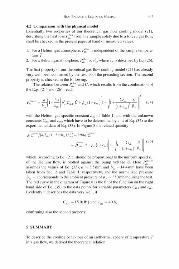
with the Helium gas specific constant bHe of Table 1, and with the unknown constants CHe1 and cHe, which have to be determined by a fit of Eq. (34) to the experimental data of Eq. (33). In Figure 8 the related quantity

P a b a b p P

C U p c

Heflow U

He He Heflow U

He He

, ,.1 3 3 90

1

2

1

−( )( ) =

= + +

∞

∞

(( ) − ++( )

∞

1 12

12

c

c

U

pHe

He

(35)

which, according to Eq. (21), should be proportional to the uniform speed v∞ of the Helium flow, is plotted against the pump voltage U. Here PHe

flow U, assumes the values of Eq. (33), a = 3.5 mm and bHe = 14 4. mm have been taken from Sec. 2 and Table 1, respectively, and the normalized pressure p∞ = 1 corresponds to the ambient pressure of p∞ = 350 mbar during the test. The red curve in the diagram of Figure 8 is the fit of the function on the right hand side of Eq. (35) to the data points for variable parameters CHe1 and cHe. Evidently it describes the data very well, if

C WHe1 15 0= . [ ] and cHe = 40 8. ,

confirming also the second property.

5 SUMMARY

To describe the cooling behaviour of an isothermal sphere of temperature T in a gas flow, we derived the theoretical relation


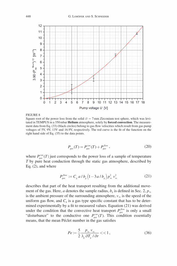
P T P T Pgas gascon

gasflow( ) ( )= + , (20)

where P Tgascon ( ) just corresponds to the power loss of a sample of temperature

T by pure heat conduction through the static gas atmosphere, described by Eq. (2), and where

P C a b a b p vgasflow

g g g: / /= −( ) ∞ ∞1 3 2 2 (21)

describes that part of the heat transport resulting from the additional move-ment of the gas. Here, a denotes the sample radius, bg is defined in Sec. 2, p∞ is the ambient pressure of the surrounding atmosphere, v∞ is the speed of the uniform gas flow, and Cg is a gas type specific constant that has to be deter-mined experimentally by a fit to measured values. Equation (21) was derived under the condition that the convective heat transport Pgas

flow is only a small “disturbance” to the conductive one P Tgas

con ( ). This condition essentially means, that the mean Péclet number in the gas satisfies

Pep v

T rg g

:/

=∂ ∂

<<∞ ∞5

21

λ, (36)

FIGurE 8Square root of the power loss from the solid ∅ = 7 mm Zirconium test sphere, which was levi-tated in TEMPuS in a 350 mbar Helium atmosphere, solely by forced convection. The measure-ment data from Eq. (33) (black circles) belong to gas flow velocities which result from gas pump voltages of 5V, 9V, 13V and 16.9V, respectively. The red curve is the fit of the function on the right hand side of Eq. (35) to the data points.


where λg is the thermal conductivity and ∂ ∂T rg / the temperature gradient in the gas. Furthermore, Eq. (21) bases on the assumption that the flow field v(x) of the compressible cooling gas can be related via Eq. (13) to the well-known “Stokes flow” vSt(x), describing the flow of an incompressible fluid around a sphere. It is remarkable, that Pgas

flow of Eq. (21) does not depend on the sample temperature T.

In our present experimental situation the gas flow is generated by a circu-lation pump driving the gas from the experiment chamber through a nozzle against the sample, see Figure 3. Since, contrary to the input voltage U of the electric pump, the speed v∞ of the uniform gas flow appearing in Eq. (21) is not directly measurable, we derived in Eq. (26) a relation between these two quantities. Inserted into Eq. (21), we finally obtained

Pa

b

a

bp C U p cgas

flow U

g gg g

, = −

+ +( ) − +∞ ∞1

31 1 1

22

1

cc

c

U

pg

g12

2

+( )

∞

, (34)

where p p∞ ∞=: / 350mbar defines the normalized ambient pressure in the experiment chamber and U U V: /= 1 the normalized pump voltage. The two positive, gas type specific constants cg g∝ η and Cg1 have to be determined by a fit to experimental values.

To check Eq. (34), we measured the temperature time behaviour of a solid spherical Zirconium sample levitated in TEMPuS under different atmo-spheric conditions (static Helium/Argon gas, Helium/Argon gas flow at dif-ferent pump voltages) within the ≈20 seconds weightlessness time of several parabolas flown during a parabolic flight mission of TEMPuS. A sketch of the sample and its environment is shown in Figure 3. Due to the weightless-ness the otherwise additionally occurring natural convection cooling in the surrounding gas atmosphere didn’t occur. It turned out, that our forced con-vection model (34) fits very well to the measured heat loss in a streaming Helium atmosphere, if the TEMPuS facility specific constants cg and Cg1 assume the values

C WHe1 15 0= . [ ] and cHe = 40 8. .

Contrary to Helium gas, the forced convection model (34) does not fit to the power loss measured in a streaming Argon atmosphere. We assume the rea-son for this in the poor thermal conductivity λAr of the Argon gas, which, according to Table 1, is by about one order of magnitude smaller than that λHe of Helium, and the resulting violation of the requirement of a small Péclet number (36). Here, we only note this result and leave the presentation of the measurement data together with a suitable theoretical description to a later publication.


Together with the results for the induced electrical power Pind (t), the power loss by radiation Prad (T(t)) and the power loss by heat conduction P T tgas

con ( ( )) (see Eq. (2)), derived in [1] and [2], Eq. (34) completes the heat balance equation (1)

m cdT t

dtP t P T t P T t P T tp

ind radgascon

gasflow( )

( ) ( ( )) ( ( )) ( ( ))= − − − ,

which, after a numerical integration, allows to predict, with sufficient accu-racy, the temperature-time behaviour of a sample levitated in the TEMPuS facility.

ACKNOWLEDGMENTS

The authors thank the space agency of the “German Aerospace Center” (DLr), bonn for enabling us to perform the experiments during the 25th DLr parabolic flight campaign 2014. Furthermore, they thank the pilots and crew members of “Novespace”, bordeaux for the almost jitter-free execution of the parabolic flights and the members of the TEMPuS team for the operation of the TEMPuS facility.

REFERENCES

[1] G. Lohöfer and I. Egry, High Temp.-High Press. 42 (2013) 175–202. [2] G. Lohöfer and S. Schneider, High Temp.-High Press. 44 (2015) 147–162. [3] J. brillo, G. Lohöfer, F. Schmidt-Hohagen, S. Schneider and I. Egry, Int. J. Materials and

Product Technology 26 (2006) 247–273. [4] D. Herlach, r. Cochrane, I. Egry, H. Fecht and L. Greer, International Materials Review 38

(1993) 273–347. [5] 25th DLR Parabolic flight campaign, 20th–31st October 2014, Practical and Technical Infor-

mation, DI-2014-ed1-en, Novespace, bordeaux-Mérignac, Mars 2014. See also: www.novespace.com.

[6] I. Egry and D. Voss, JASMA 27 (2010) 178–182. [7] G. Lohöfer and J. Piller, Proc. 40th AIAA Aerospace Sciences Meeting & Exhibit, 14.–17.

January 2002, reno, u.S.A, paper no.: AIAA 2002–0764. [8] N. D. Milosevic and K. D. Maglic, Int. J. Thermophys. 27 (2006) 1140–1159. [9] D. r. Kassoy, T. C. Adamson and A. F. Messiter, Phys. Fluids 9 (1966) 671–681.[10] H. D. baehr and K. Stephan, Heat and Mass Transfer, Springer, berlin 2011.[11] E. Guyon, J.-P. Hulin, L. Petit and C. D. Mitescu, Physical Hydrodynamics, Oxford

university Press, New York, 2001.[12] N. Mohan, T. M. undeland and W. P. robins, Power Electronics, 3rd ed., Wiley, New York,

2003.

heat balance in levitation melting: sample cooling by ... balance in levitation melting... · of...

Documents