hawkes learning systems math courseware specialists discovering relationships chapter 5 copyright ©...

HAWKES LEARNING SYSTEMS

math courseware specialists

Discovering Relationships

Chapter 5

Copyright © 2010 by Hawkes Learning

Systems/Quant Systems, Inc.

All rights reserved.





Objectives:

• Creating a scatter plot.• Calculating the correlation coefficient.


Sections 5.2-5.5 Scatter Plots and Correlation



• In previous chapters, the statistical summary measurements, like the mean, variance, and proportions, were all concerned with describing univariate data (measurements from one variable).

• To understand the relationship between two variables, data on both variables need to be collected. This type of data is called bivariate data.

• With bivariate data, two observations are recorded from some entity.

• Important questions to ask yourself when you encounter bivariate data:

• How was the data obtained?• What exactly does the data measure?• Is the data measured accurately?


Section 5.1 Bivariate Data

Bivariate Data:



• Detecting a relationship between two variables often begins with a graph.

• In the case of bivariate data, a scatterplot is the traditional explanatory graphical method to display the relationship between two variables.• In a scatterplot, measurements are plotted in pairs with one variable plotted on each axis.• When examining the scatterplot we are trying to draw conclusions concerning the overall pattern of the data.

• Questions to ask yourself when analyzing a scatterplot:

Does the pattern roughly follow a line?Is the pattern upward sloping or downward sloping?

Are the data values tightly clustered or widely dispersed?Are there significant deviations from the pattern?

Scatterplot:


Section 5.2 Looking for Patterns in the Data



x

y y

x

• In these two scatterplots the data are strongly related and fall in a straight line.• In the scatterplot to the left the slope is positive, meaning as the X variable increases the Y variable increases as well.• In the plot to the right the relationship is negative; as the X variable increases, the Y variable decreases. • This is also called an inverse relationship.



Strong Relationships:



y

x

y

x

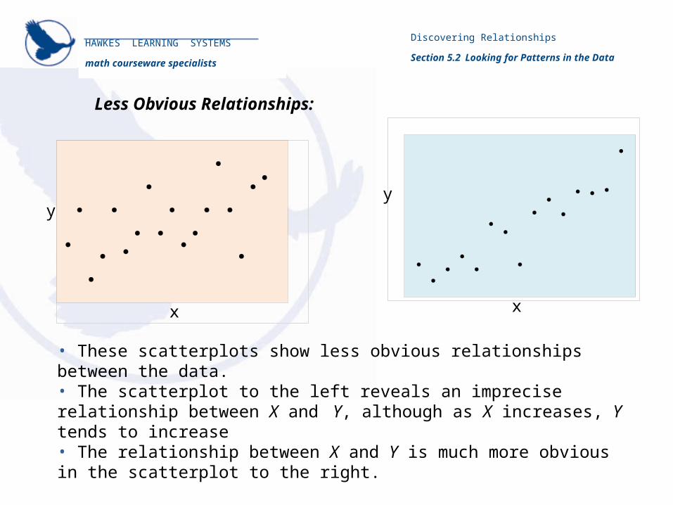
• These scatterplots show less obvious relationships between the data.• The scatterplot to the left reveals an imprecise relationship between X and Y, although as X increases, Y tends to increase• The relationship between X and Y is much more obvious in the scatterplot to the right.



Less Obvious Relationships:



• The scatterplot to the left reveals a downward sloping relationship between X and Y.• The relationship is not as exact as we saw earlier with the straight lines.• The right scatterplot has no apparent relationship between X and Y.

x x

y y



Less Obvious Relationships:



• Consider the problem of deciding how long to study for an upcoming test.

• If we knew the exact relationship between time spent studying and the grade received, it could be useful in allocating study time.

• One method of defining a precise relationship between two or more variables is with the use of a mathematical model.

• Suppose, for example, the relationship between test and study time was given by the linear equation below:

Test Score = 45 + 3.8 (hours of study time).


Section 5.3 Building a Model

Building a Model:



Test Score = 45 + 3.8 (hours of study time)

• If this mathematical model is accurate, then anyone would be able to control his/her destiny. If a person only studied 10 hours, according to the model his/her test score would be:

Test Score = 45 + 3.8 (10) = 83.

• If this score is not high enough, then study 12 hours:

Test Score = 45 + 3.8 (12) = 90.6.

• If you had to make a 95 on the test, how many hours do you have to study?

95 = 45 + 3.8 (hours of study time)

hours of study time =



Building a Model:

95 4513.16.

3.8



• Sorry folks, but there is no model that can precisely predict a test score just on the basis of time studied; there are many variables that affect your test score.

• But suppose there was a model which, though imperfect, fairly reliably predicted test scores based on the hours studied.

Test Score = 45 + 3.8 (hours of study time) + error

• The new model admits the possibility of error. Now if someone studies 10 hours, the model would predict

Test Score = 45 + 3.8 (10) = 83 + error



Error in a Model:



• A linear relationship is graphically described as a line.

• Mathematically, a line is a set of points that satisfy the functional relationship

where m is the slope of the line and b is the point where the function crosses the Y-axis, which is called the Y-intercept.

y mx b

• If two variables appear be related in a straight line manner, we can use a linear equation to model their relationship.

• Very few observed relationships are exactly linear, although most follow an inexact linear pattern.



Linear Relationship:



The relationship in the figure above is the linear equationy = 5x + 3.

In this case m = 5 and b = 3.

Together the slope and the intercept are called the parameters of a linear equation. That is, they completely define the equation of the line.

y =

mx

+

b

b

y

x

The slope determines if the line slopes upward (positive slope) or if the line slopes downward (negative slope).



Linear Equation:



When linear relationships exist, the data will have a tendency to move together.

As X increases, Y increases As X increases, Y decreases

As X increases, Y does not change in a predictable way



Linear Relationships:



• A scatter diagram is a useful exploratory tool for detecting relationships between two variables.• Eventually a researcher will want to know the strength of the relationship between the two variables• Karl Peterson developed the correlation coefficient, r, to measure the degree of linear relationship. • The correlation coefficient is an index number used to summarize the strength of the linear relationship.

1

1

1

ni i

i x y

x x y yr

n s s

1 1r

Do and look familiar?i i

x y

x x y ys s


Section 5.4 Measuring the Degree of Linear Relationship

Correlation Coefficient:



is a - score that shows how far deviates

from its mean.

i

y

y yz y

s

is a score that shows how far deviates

from its mean.

i

x

x xz - x

s

• Both are measured in standard deviation units.

• Summing the products of these deviation measures for each data pair determines the sign of the correlation coefficient.

• It does not matter whether you sum Y with X or X with Y; you will still get the same value of r.



Deviation Measures:



• When r is positive, there is a tendency for Y to increase as X increases.

• If both of the deviations are positive, then each of the observations is above the mean.

• If both are negative, the each is below the mean.

• When one of the variables is above its mean, the other variable tends to be above its mean.

• If one variable is below its mean, the other tends to be below its mean.

Positive Relationships:





The mean of x

The mean of Y

Points below the means of X and Y

Points above the means of X and Y

In group A, since the deviations are positive and are positive,

the expression is positive.

i i

i i

x y

x x y y

x x y y

s s

In group B, since the deviations are negative and are negative,

the expression is positive.

i i

i i

x y

x x y y

x x y y

s s



Positive Relationship:



The mean of x

The mean of Y

Points above the mean of X, below the mean of Y

Points below the mean of X, above the mean of Y

In group C, since the deviations are negative and are positive,

the expression is negative.

i i

i i

x y

x x y y

x x y y

s s

In group D, since the deviations are positive and are negative,

the expression is negative.

i i

i i

x y

x x y y

x x y y

s s



Negative Relationship:



• The correlation coefficient, r, measures the degree of linear relationship.

• The value of r is always between −1 and 1.

• A value of r near − 1 or +1 means the data is tightly bundled around a line.

• A value of r near − 1 or +1 means that it would be very easy to predict one of the variables by using the other.

• Positive association is indicated by a plus sign and an upward sloping relationship.

• Negative association is indicated by a minus sign and a negatively sloping relationship.

• A value of r near zero means there is no linear relationship.



Properties of the Correlation Coefficient:



• Suppose that a high correlation has been observed between the weekly sales of ice cream and the number of snake bites each week. It seems unlikely that ice cream sales would cause snakes to bite people or that more snake bites would cause higher ice cream sales.

• The apparent relationship is an illusion caused by a phenomenon called common response. This means that both variables are related to a third variable.

• A high correlation does not imply causation.

Correlation Pitfalls:


Section 5.5 Avoiding Some Correlation Pitfalls



• Correlating summary measures (such as means) will tend to provide an inflated correlation measurement.

• Ignoring the variation of the individual values magnifies the correlation measure and gives a somewhat distorted view of the underlying relationship.

• Suppose there is a good reason to believe that a causal relationship exists between two variables, but when a correlation is performed the value of the correlation is near zero, indicating no association.

• A low correlation could indicate that no linear relationship exists.

Correlation Pitfalls:





In the figure above, the relationship between X and Y is not a straight line. The correlation measure for these points is going to be very close to zero. Yet there does appear to be a strong relationship between X and Y. The kind of relationship exhibited by this data is called a quadratic relationship.

Nonlinear Relationship:





For example:• The variable Y is dependent on X. As X changes, Y changes.• Such a relationship should produce a significant correlation

measure.• But also suppose there is another variable Z, which also affects Y. • As Z changes so does Y. Changes in Z could mask the changes

caused by X.

XY

Z



Confounding:

• Another problem that can produce low correlations is confounding. Confounding occurs when more than one variable affects the dependent variable.





• Finding the Least Squares Line• Determining the slope of the line.• Calculating the y-intercept of the line.• Evaluating the fit of the model.


Sections 5.6-5.9 Fitting a Linear Model

Objectives:



• In the previous section the correlation coefficient is used to measure the degree of linear relationship between two variables.

• However, the correlation coefficient does not describe the exact linear association between X and Y.

• Regression analysis determines the specific relationship between X and Y.

• Using regression analysis we may be able to use X to predict Y.


Section 5.6 Defining a Linear Relationship – Regression

Analysis

Regression Analysis:



• Recall, the equation of a line is

.y mx b m slopeb - intercept y

• However, traditional statistics uses different symbols for the slope and intercept in the equation of a line. Instead of , let be the symbol used to describe the y-intercept and be the symbol used to represent the slope of the line.

0bb1b

• Using this new set of symbols, the equation of the line becomes

0 1 .y b b x




Analysis



• The linear equation relation X to Y is referred to as a mathematical model.

Y is called the dependent variable. X is called the independent variable.

• Now we are ready to look at examples of linear relationships.



Analysis




• Let b0=3 and b1=2, this specifies the line Y = 3 + 2X.

• Let b0= 8 and b1= −2, this specifies the line Y = 8 − 2X.

Example:



Analysis



What about fitting a line to this data set.Does line A fit the data?

What about B? C?

To find the best line, we need to come up with a method of summarizing how close each line is to the data.



Analysis

Defining a Linear Relationship:



Observed value

If we plug in x=4 in our model we get

X Y

2 3

4 2

5 6

8 5

9 8

The data to the left was plotted in the plot to the

right.

Next, try to draw a line through the points.No straight line passes through the points.

However, Y = 1 + 0.7X seems to fit the data reasonably well.

How well does the line fit the data?



Analysis

Defining a Linear Relationship:



• To determine how well the line fits the data, first we need to look at the error.

• Error = observed Y – predicted Y = 2 – 3.8 = – 1.8.Using symbols,

• The error reflects how far each observation is from the line. Examining the errors suggests how well the line fits the data, but negative error can cancel out positive error.

• By squaring the error, we get positive data that can be used as a criterion for selecting the best fitting line.

ˆy y error 2 3.8 1.8.

ˆ y y observed and predicted , soY Y



Analysis

Error:



22 2

0 1ˆSSE error i i i iiy y y b b x

• SSE can be used as a criterion for selecting the best fitting line through a set of points. If SSE is zero, then the model fits the data exactly and the observed data must lie in a straight line.

• If line A’s SSE is larger than line B’s then line B fits the data better than line A.

• The best line is called the Least Squares Line, and has the smallest SSE.



Analysis

Sum of Squared Errors (SSE):



Observed versus Predicted Values

Observed Observed Predicted Y Error2

2 3 4 2 5 6 8 5 9 8

YX2.4 = 1 + 0.7(2)

3.8 = 1 + 0.7(4)

4.5 = 1 + 0.7(5)

6.6 = 1 + 0.7(8)

7.3 = 1 + 0.7(9)

3 – 2.4 = +0.6

2 – 3.8 = – 1.8

6 – 4.5 = +1.5

5 – 6.6 = – 1.6

8 – 7.3 = +0.7

error 0.6 = 2SSE error 8.90

0.36

3.24

2.25

2.56

0.49

Use this chart to determine the distance from the observed points to the line Y = 1 + 0.7X.

ˆ Y Y error ˆ 1 .7Y X



Analysis

Example:



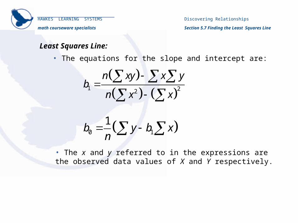
1 22

n xy x yb

n x x

0 1

1b y b x

n

• The equations for the slope and intercept are:

• The x and y referred to in the expressions are the observed data values of X and Y respectively.


Section 5.7 Finding the Least Squares Line

Least Squares Line:



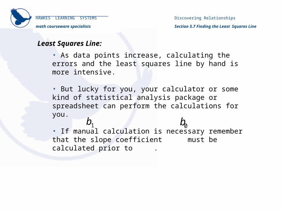
• As data points increase, calculating the errors and the least squares line by hand is more intensive.

• But lucky for you, your calculator or some kind of statistical analysis package or spreadsheet can perform the calculations for you.

• If manual calculation is necessary remember that the slope coefficient must be calculated prior to .0b1b


Section 5.7 Finding the Least Squares Line

Least Squares Line:

hawkes learning systems math courseware specialists discovering relationships chapter 5 copyright ©...

Documents