has the business cycle changed and why? - nber.org · department of economics and the woodrow...
TRANSCRIPT
This PDF is a selection from a published volumefrom the National Bureau of Economic Research
Volume Title: NBER Macroeconomics Annual 2002,Volume 17
Volume Author/Editor: Mark Gertler and KennethRogoff, editors
Volume Publisher: MIT Press
Volume ISBN: 0-262-07246-7
Volume URL: http://www.nber.org/books/gert03-1
Conference Date: April 5-6, 2002
Publication Date: January 2003
Title: Has the Business Cycle Changed and Why?
Author: James H. Stock, Mark W. Watson
URL: http://www.nber.org/chapters/c11075
James H. Stock and Mark W. Watson DEPARTMENT OF ECONOMICS AND THE KENNEDY SCHOOL OF GOVERNMENT, HARVARD UNIVERSITY, AND NBER; AND DEPARTMENT OF ECONOMICS AND THE WOODROW WILSON SCHOOL, PRINCETON UNIVERSITY, AND NBER
Has the Business Cycle Changed and Why?
1. Introduction The U.S. economy has entered a period of moderated volatility, or quies- cence. The long expansion of the 1990s, the mild 2001 recession, and the current moderate recovery reflect a trend over the past two decades to- wards moderation of the business cycle and, more generally, reduced vol- atility in the growth rate of GDP.
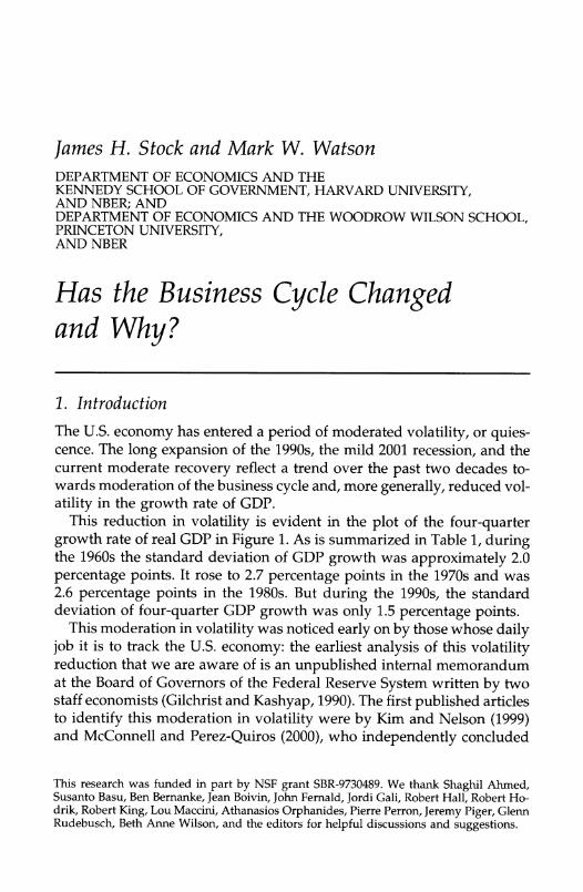
This reduction in volatility is evident in the plot of the four-quarter growth rate of real GDP in Figure 1. As is summarized in Table 1, during the 1960s the standard deviation of GDP growth was approximately 2.0 percentage points. It rose to 2.7 percentage points in the 1970s and was 2.6 percentage points in the 1980s. But during the 1990s, the standard deviation of four-quarter GDP growth was only 1.5 percentage points.
This moderation in volatility was noticed early on by those whose daily job it is to track the U.S. economy: the earliest analysis of this volatility reduction that we are aware of is an unpublished internal memorandum at the Board of Governors of the Federal Reserve System written by two staff economists (Gilchrist and Kashyap, 1990). The first published articles to identify this moderation in volatility were by Kim and Nelson (1999) and McConnell and Perez-Quiros (2000), who independently concluded
This research was funded in part by NSF grant SBR-9730489. We thank Shaghil Ahmed, Susanto Basu, Ben Beranke, Jean Boivin, John Femald, Jordi Gali, Robert Hall, Robert Ho- drik, Robert King, Lou Maccini, Athanasios Orphanides, Pierre Perron, Jeremy Piger, Glenn Rudebusch, Beth Anne Wilson, and the editors for helpful discussions and suggestions.
160 * STOCK & WATSON
Figure 1 ANNUAL GROWTH RATES OF GDP
v- i i
0 l
I I I I I I I I
1960 1965 1970 1975 1980 1985 1990 1995 2000 2005
Year
Table 1 SUMMARY STATISTICS FOR FOUR-QUARTER GROWTH IN REAL GDP, 1960-2001
Sample period Mean (%) Standard deviation (%)
1960-2001 3.3 2.3 1960-1969 4.3 2.0 1970-1979 3.2 2.7 1980-1989 2.9 2.6 1990-2001 3.0 1.5
Notes: Summary statistics are shown for 100 x ln(GDP,/GDPt 4), where GDP, is the quarterly value of real GDP.
that there was a sharp decline, or break, in the volatility of U.S. GDP growth in the first quarter of 1984. The moderation was also documented by Simon (2000). These papers have stimulated a substantial recent litera- ture, much of it yet unpublished, that characterizes this decline in volatil- ity and searches for its cause.1
1. See Ahmed, Levin, and Wilson (2002), Basistha and Startz (2001), Blanchard and Simon (2001), Boivin and Giannoni (2002a, 2002b), Chauvet and Potter (2001), Feroli (2002), Go-
I I
I /
Has the Business Cycle Changed and Why? ? 161
This article has two objectives. The first is to provide a comprehensive characterization of the decline in volatility using a large number of U.S. economic time series and a variety of methods designed to describe time-
varying time-series processes. In so doing, we review the literature on the moderation and attempt to resolve some of its disagreements and discrep- ancies. This analysis is presented in Sections 2, 3, and 4. Our empirical analysis and review of the literature leads us to five conclusions:
1. The decline in volatility has occurred broadly across the U.S. economy: since the mid-1980s, measures of employment growth, consumption growth, and sectoral output typically have had standard deviations 60% to 70% of their values during the 1970s and early 1980s. Fluctua- tions in wage and price inflation have also moderated considerably.
2. For variables that measure real economic activity, the moderation
generally is associated with reductions in the conditional variance in time-series models, not with changes in the conditional mean; in the
language of autoregressions, the variance reduction is attributable to a smaller error variance, not to changes in the autoregressive coefficients. This conclusion is consistent with the findings of Ahmed, Levin, and Wilson (2002), Blanchard and Simon (2001), Pagan (2000), and Sensier and van Dijk (2001).
3. An important unresolved question in the literature is whether the mod- eration was a sharp break in the mid-1980s, as initially suggested by Kim and Nelson (1999) and McConnell and Perez-Quiros (2000), or
part of an ongoing trend, as suggested by Blanchard and Simon (2001). In our view the evidence better supports the break than the trend char- acterization; this is particularly true for interest-sensitive sectors of the
economy such as consumer durables and residential investment. 4. Both univariate and multivariate estimates of the break date center on
1984. When we analyze 168 series for breaks in their conditional vari- ance, approximately 40% have significant breaks in their conditional variance in 1983-1985. Our 67% confidence interval for the break date in the conditional variance of four-quarter GDP growth (given past values of GDP growth) is 1982:4 to 1985:3, consistent with Kim and Nelson's (1999) and McConnell and Perez-Quiros's (2000) estimate of 1984:1.
5. This moderation could come from two nonexclusive sources: smaller unforecastable disturbances (impulses) or changes in how those distur-
lub (2000), Herrera and Pesavento (2002), Kahn, McConnel, and Perez-Quiros (2001), Kim, Nelson, and Piger (2001), Pagan (2000), Primiceri (2002), Ramey and Vine (2001), Sensier and van Dijk (2001), Simon (2001), Sims and Zha (2002), and Wamock and Warnock (2001). These papers are discussed below in the context of their particular contribution.
162 * STOCK & WATSON
bances propagate through the economy (propagation). Although the propagation mechanism (as captured by VAR lag coefficients) ap- pears to have changed over the past four decades, these changes do not account for the magnitude of the observed reduction in vola-
tility. Rather, the observed reduction is associated with a reduction in the magnitude of VAR forecast errors, a finding consistent with the multivariate analyses of Ahmed, Levin, and Wilson (2002), Boivin and Giannoni (2002a, 2002b), Primiceri (2002), Simon (2001), and Sims and Zha (2002), although partially at odds with Cogley and Sargent (2002).
The second objective of this article is to provide new evidence on the
quantitative importance of various explanations for this "great modera- tion." These explanations fall into three categories. The first category is
changes in the structure of the economy. Candidate structural changes include the shift in output from goods to services (Burns, 1960; Moore and Zarnowitz 1986), information-technology-led improvements in inventory management (McConnell and Perez-Quiros, 2000; Kahn, McConnel, and Perez-Quiros, 2001, 2002), and innovations in financial markets that facili- tate intertemporal smoothing of consumption and investment (Blanchard and Simon, 2001). The second category is improved policy, in particular improved monetary policy (e.g., Taylor, 1999b; Cogley and Sargent, 2001), and the third category is good luck, that is, reductions in the variance of
exogenous structural shocks. We address these explanations in Section 5. In brief, we conclude that
structural shifts, such as changes in inventory management and financial markets, fail to explain the timing and magnitude of the moderation docu- mented in Sections 2-4. Changes in U.S. monetary policy seem to account for some of the moderation, but most of the moderation seems to be attrib- utable to reductions in the volatility of structural shocks. Altogether, we estimate that the moderation in volatility is attributable to a combination of improved policy (10-25%), identifiable good luck in the form of pro- ductivity and commodity price shocks (20-30%), and other, unknown forms of good luck that manifest themselves as smaller reduced-form forecast errors (40-60%); as discussed in Section 5, these percentages have
many caveats.
2. Reductions in Volatility throughout the Economy This section documents the widespread reduction in volatility in the 1990s and provides some nonparametric estimates of this reduction for 22 major economic time series. We begin with a brief discussion of the data.
Has the Business Cycle Changed and Why? * 163
2.1 DATA AND TRANSFORMATIONS
In all, we consider data on 168 quarterly macroeconomic time series from 1959:1 to 2001:3. The U.S. data represent a wide range of macroeco- nomic activity and are usefully grouped into six categories: (1) NIPA de-
compositions of real GDP, (2) money, credit, interest rates, and stock
prices, (3) housing, (4) industrial production, (5) inventories, orders, and sales, (6) employment. In addition, we consider industrial production for five other OECD countries. Seasonally adjusted series were used when available.
Most of our analysis uses these quarterly data, transformed to eliminate trends and obvious nonstationarity. Specifically, most real variables were transformed to growth rates (at an annual rate), prices and wages were transformed to changes in inflation rates (at an annual rate), and interest rates were transformed to first differences. For some applications (such as the data description in Section 2.2) we use annual growth rates or annual differences of the quarterly data. For variable transformed to growth rates, say Xt, this means that the summary statistics are reported for the series 100 x ln(Xt/X -4). For prices and wages, the corresponding transfor- mation is 100 X [ln(Xt/Xt-l)
- ln(Xt-4/Xt-5)], and for interest rates the transformation is Xt - Xt-4. Definitions and specific transformations used for each series are listed in Appendix B.
2.2 HISTORICAL VOLATILITY OF MAJOR ECONOMIC TIME SERIES
2.2.1 Volatility by Decade Table 2 reports the sample standard deviation of 22 leading macroeconomic time series by decade (2000 and 2001 are included in the 1990s). Each decade's standard deviation is presented rela- tive to the full-sample standard deviation, so a value less than one indi- cates a period of relatively low volatility. All series were less volatile in the 1990s than over the full sample, and all but one series (consumption of nondurables) were less volatile in the 1990s than in the 1980s. On the demand side, the 1990 relative standard deviations ranged from 0.65 (gov- ernment spending and residential investment) to 0.89 (nonresidential in- vestment). On the production side, the standard deviations during the 1990s, relative to the full sample, range from 0.65 (durable goods produc- tion) to 0.87 (services). Comparable volatility reductions are found when standard deviations are compared before and after the 1984:I break date of Kim and Nelson (1999) and McConnell and Perez-Quiros (2000) (Table 2, final column).
This decline in volatility is reflected in other series as well. For example, the relative standard deviation of annual growth of nonagricultural em-
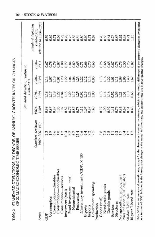
Table 2 STANDARD DEVIATIONS, BY DECADE, OF ANNUAL GROWTH RATES OR CHANGES OF 22 MACROECONOMIC TIME SERIES
Standard deviation, relative to 1960-2001
Standard deviation Standard deviation 1960- 1970- 1980- 1990- 1984-2001,
Series 1960-2001 (%) 1969 1979 1989 2001 relative to 1960-1983
GDP Consumption
Consumption-durables Consumption-nondurables Consumption-services
Investment (total) Fixed investment-total
Nonresidential Residential
A(inventory investment) / GDP, x 100 Exports Imports Government spending
Production Goods (total)
Nondurable goods Durable goods
Services Structures
Nonagricultural employment Price inflation (GDP deflator) 90-day T-bill rate 10-year T-bond rate
2.3 1.9 6.6 1.8 1.2
10.4 6.7 6.7
13.4 0.6 6.4 7.2 2.5
3.6 7.3 2.5 1.1 6.2 1.7 0.4 1.7 1.2
0.98 1.18 0.97 1.17 0.87 1.18 1.06 1.22 1.07 0.84 0.82 1.15 0.77 1.29 0.87 1.17 0.78 1.25 1.12 0.92 1.07 1.13 0.87 1.24 1.40 1.00
0.97 1.13 1.00 1.14 0.92 1.16 1.41 0.52 0.73 1.33 0.94 1.21 0.69 1.51 0.51 1.10 0.43 0.65
1.14 0.67 1.07 0.78 1.13 0.79 0.81 0.87 1.20 0.88 1.22 0.77 1.04 0.84 1.06 0.89 1.23 0.65 1.22 0.71 1.12 0.66 1.14 0.70 0.85 0.65
1.13 0.76 1.16 0.68 1.22 0.65 1.01 0.87 1.11 0.73 1.09 0.73 1.06 0.50 1.43 0.75 1.67 0.82
Notes: NIPA series are annual growth rates, except for the change in inventory investment, which is the annual difference of the quarterly change in inventories as a fraction of GDP. Inflation is the four-quarter change in the annual inflation rate, and interest rates are in four-quarter changes.
z V3 R RO
0_>
6 0.59 0.62 0.71 0.66 0.73 0.78 0.75 0.87 0.52 0.80 0.60 0.71 0.69
0.70 0.63 0.61 0.73 0.67 0.62 0.48 0.71 1.13
Has the Business Cycle Changed and Why? ? 165
ployment in the 1990s was 0.73. The 1990s were also a period of quies- cence for inflation: changes in annual price inflation, measured by the GDP deflator, has a relative standard deviation of 0.50. As noted by Kim, Nelson, and Piger (2001), Watson (1999), and Basistha and Startz (2001), the situation for interest rates is somewhat more complex. Although the variance of interest rates decreased across the term structure, the decrease was more marked at the short than at the long end, that is, the relative
volatility of long rates increased.
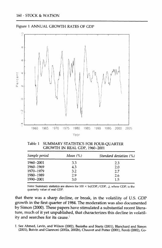
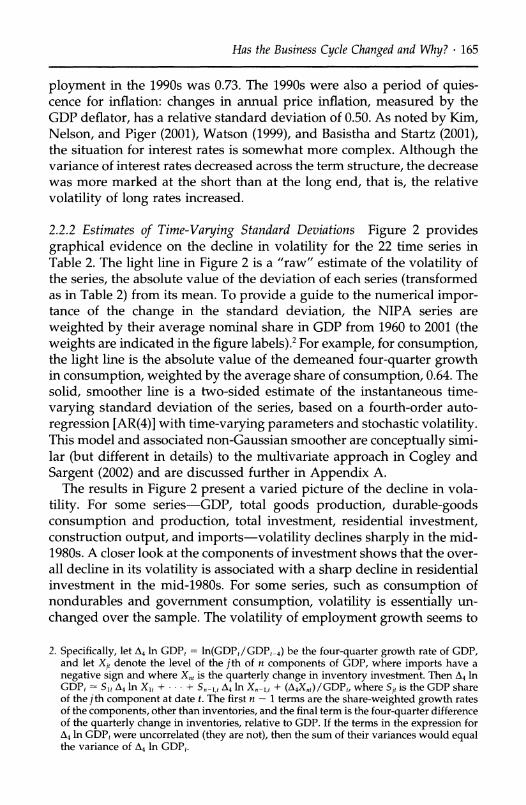
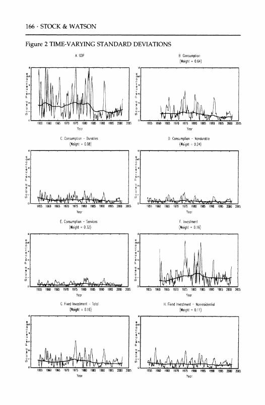
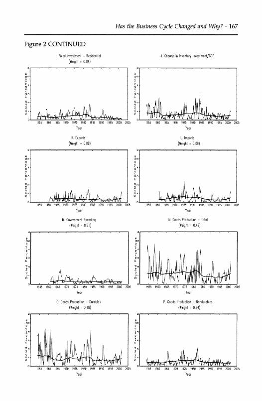
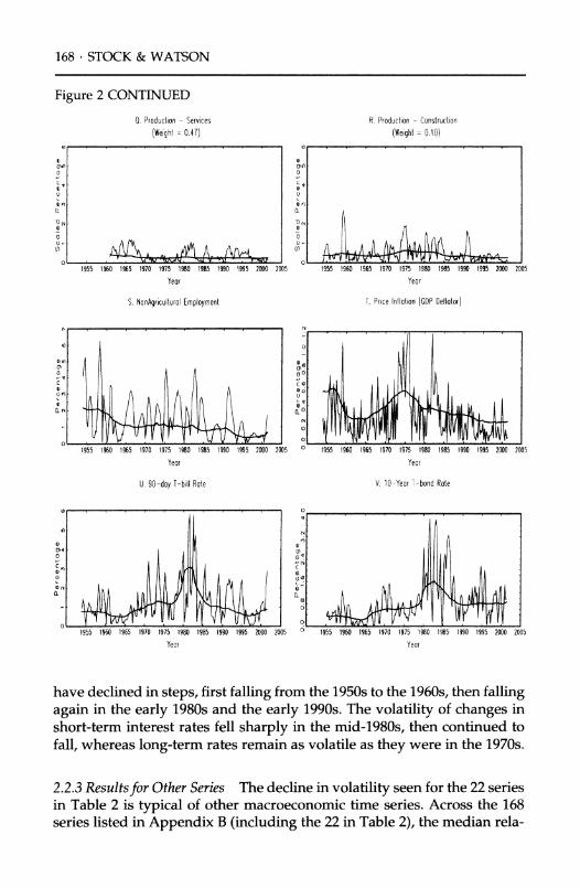
2.2.2 Estimates of Time-Varying Standard Deviations Figure 2 provides graphical evidence on the decline in volatility for the 22 time series in Table 2. The light line in Figure 2 is a "raw" estimate of the volatility of the series, the absolute value of the deviation of each series (transformed as in Table 2) from its mean. To provide a guide to the numerical impor- tance of the change in the standard deviation, the NIPA series are
weighted by their average nominal share in GDP from 1960 to 2001 (the weights are indicated in the figure labels).2 For example, for consumption, the light line is the absolute value of the demeaned four-quarter growth in consumption, weighted by the average share of consumption, 0.64. The solid, smoother line is a two-sided estimate of the instantaneous time-
varying standard deviation of the series, based on a fourth-order auto-
regression [AR(4)] with time-varying parameters and stochastic volatility. This model and associated non-Gaussian smoother are conceptually simi- lar (but different in details) to the multivariate approach in Cogley and
Sargent (2002) and are discussed further in Appendix A. The results in Figure 2 present a varied picture of the decline in vola-
tility. For some series-GDP, total goods production, durable-goods consumption and production, total investment, residential investment, construction output, and imports-volatility declines sharply in the mid- 1980s. A closer look at the components of investment shows that the over- all decline in its volatility is associated with a sharp decline in residential investment in the mid-1980s. For some series, such as consumption of nondurables and government consumption, volatility is essentially un-
changed over the sample. The volatility of employment growth seems to
2. Specifically, let A4 In GDPt = ln(GDP,/GDPt-4) be the four-quarter growth rate of GDP, and let Xjt denote the level of the jth of n components of GDP, where imports have a negative sign and where X,, is the quarterly change in inventory investment. Then A4 In GDPt I Sl A4 In X1t + * * + Sn,-,t A4 In Xn -, + (A4Xnt)/GDPt, where Sj, is the GDP share of the jth component at date t. The first n - 1 terms are the share-weighted growth rates of the components, other than inventories, and the final term is the four-quarter difference of the quarterly change in inventories, relative to GDP. If the terms in the expression for A4 In GDPt were uncorrelated (they are not), then the sum of their variances would equal the variance of A4 In GDP,.
166 * STOCK & WATSON
Figure 2 TIME-VARYING STANDARD DEVIATIONS
A. GOP
v 0 0 c o)
D o o o
-D 0 (/
Year
C. Consumption - Durobles
(Weight = 0.08) ?
.
,, I
. .
a>1
o
o om Cn
0 0u
1
V)
1955 1960 1965 1970 1975 1980 1985 1990 1995 2000 2
Yeor
E. Consumption - Services
(Weight = 0.32)
B. Consumption (Weight 0.64)
1955 1960 1965 1970 1975 1980 1985 1990 1995 2000 20(
Year
. Consumption - Nonduroble
(Weight = 0.24)
m) o
0
or
o_
0
U)
1955 1960 1965 1970 1975 1980 1985 1990 1995 2000 2005
Year
F. Investment
(Weight = 0.16)
o 0t
c
a- 1L
1955 1960 1965 1970 1975 1980 1985 1990 1995 2000
Yeor
2005
G. Fixed Investment - Totol
(Weight =0.16) . . . . . . . . .
1960 1965 1970 1975 1980 1985 1990 1995 2000
Yeor
H. Fixed Investment - Nonresidentiol
(Weight =0.11)
o
a
N) ( t~
1955 1960 1965 1970 1975 1980 1985 1990 1995 2000
Year 2005 1955 1960 1965 1970 1975 1980 1985 1990 1995 2000 2005
Year
o
o
ur
1
fC. a- Dn 0
N . . . .... . .-.. .. . ..... O I '.. 1 ....-.. IV . , -
UJ . ,,I.
V . . . . . ... .. . . . . . ..
w , . 1 .
u .. . . . . O .* -. . . . . . ... .
.
vi AMA'1iAL\,AP
Has the Business Cycle Changed and Why? ? 167
Figure 2 CONTINUED
I. Fixed Investment - Residential
(Weight = 0.04)
o
0
o OUn
D
O-
_ ()
A4~~AAA, AVN.- 1955 1960 1965 1970 1975 1980 1985 1990 1995 2000 2005
Year
K. Exports (Weight = 0.08)
J. Change in Inventory Investment/GOP
0 0)'n
c 1
u
u - (nov&
1955 1960 1965 1970 1975 1980 1985 1990 1995 2000 2005
Year
L. Imports (Weight = 0.09)
o o
o
0 5
1)
0
u (f)
ID)
N-
1955 1960 1965 1970 1975 1980 1985 1990 1995 2000 200"
Year
M. Government Spending (Weight= 021)
nu-
,n
1955 1960 1965 1970 1975 1980 1985 1990 1995 2000 200
Year
0. Goods Production - Durables
(Weight = 0.18)
in .......
1955 1960 1965 1970 1975 1980 1985 1990 1995 2000 200
Year
N. Goods Production - Total
(Weight = 0.42)
i) I
1955 1960 1965 1970 1975 1980 1985 1990 1995 2000 20(
Year
P. Goods Production - Nondurables
(Weight 0.24) uo....
o
u L o)
cN 0u t A.I
Year 1955 1960 1965 1970 1975 1980 1985 1990 1995 2000 2005
Year
o
o
n
0
o1
t0
a-
U)
,u . . . . . to
r) .. I . . - ? ,- * I ./ I- .
I . I , I ..... - . .I .
O , ' I r I ,
. I . I v . IY w I,
- ,
5
c
aI c
a
5
168 STOCK & WATSON
Figure 2 CONTINUED
O. Production -Services
(Weight 0.47)
D o De- Of1
'U Cdr )
- o
Q_
1955 1960 1965 1970 1975 1980 1985 1990 1995 2000 2005
Year
S. NonAgriculturol Employment
R. Production - Construction
(Weight - 0.10)
LAV 4\fV I 1955 1960 1965 1970 1975 1980 1985 1990 1995 2000
Year
I. Price Inflation (GDP Deflotor)
20
Yeor Year
U. 90-doy T-bill Rote V. 10-Year T-bond Rate
Yeor Year
have declined in steps, first falling from the 1950s to the 1960s, then falling again in the early 1980s and the early 1990s. The volatility of changes in short-term interest rates fell sharply in the mid-1980s, then continued to fall, whereas long-term rates remain as volatile as they were in the 1970s.
2.2.3 Resultsfor Other Series The decline in volatility seen for the 22 series in Table 2 is typical of other macroeconomic time series. Across the 168 series listed in Appendix B (including the 22 in Table 2), the median rela-
t o o Q. t1 c I c
0.
ili
15
Has the Business Cycle Changed and Why? * 169
tive standard deviation in the 1990s is 0.73, and 78% of the series had a relative standard deviation less than 0.85 in the 1990s. For example, the relative standard deviation of the overall index of industrial production in the 1990s was 0.63; this reduction is also found in the various industrial
production sectors, with sectoral relative standard deviations ranging from 0.59 (consumer goods) to 0.77 (utilities). Orders and inventories showed a similar decline in volatility; the average relative standard devia- tion was 0.68 for these series in the 1990s. As discussed in more detail by Wamock and Wamock (2001), the standard deviation of employment also fell in most sectors (the exceptions being contract construction, FIRE, services, and wholesale and retail trade, where the relative standard de- viations are close to one). Although broad measures of inflation show marked declines in volatility, some producer prices showed little decrease or an increase in volatility, and the overall index of producer prices has a relative standard deviation close to one.
Finally, as discussed in Blanchard and Simon (2001) and Simon (2001), the decrease in volatility is not unique to the United States. The relative standard deviation of industrial production indexes for several other de-
veloped countries were low in the 1990s. However, some countries
(France, Japan, and Germany) also experienced low variability in the 1980s and experienced somewhat more variability in the 1990s.
2.2.4 Implicationsfor Recessions and Expansions Because recessions are de- fined as periods of absolute decline in economic activity, reduced volatil-
ity with the same mean growth rate implies fewer and shorter recessions. As discussed further by Kim and Nelson (1999), Blanchard and Simon
(2001), Chauvet and Potter (2001), and Pagan (2000), this suggests that the decrease in the variance of GDP has played a major role in the in- creased length of business-cycle expansions over the past two decades.
2.3 SUMMARY
The moderation in volatility in the 1990s is widespread (but not universal) and appears in both nominal and real series. When the NIPA series are
weighted by their shares in GDP, the decline in volatility is most pro- nounced for residential investment, output of durable goods, and output of structures. The decline in volatility appears both in measures of real economic activity and in broad measures of wage and price inflation. For the series with the largest declines in volatility, volatility seems to have fallen sharply in the mid-1980s, but to draw this conclusion with confi- dence we need to apply some statistical tests to distinguish distinct breaks from steady trend declines in volatility, a task taken up in the next section.
170 * STOCK & WATSON
3. Dating the Great Moderation The evidence in Section 2 points toward a widespread decline in volatil-
ity throughout the economy. In this section, we consider whether this decline is associated with a single distinct break in the volatility of these series and, if so, when the break occurred. We study the issue of a break in the variance, first using univariate methods, and then using multivari- ate methods. We begin by examining univariate evidence on whether the change in the variance is associated with changes in the conditional mean of the univariate time-series process or changes in the conditional variance.
3.1 CHANGES IN MEAN VS. CHANGES IN VARIANCE: UNIVARIATE EVIDENCE
The changes in the variance evident in Figure 2 could arise from changes in the autoregressive coefficients (that is, changes in the conditional mean of the process, given its past values), changes in the innovation variance (that is, changes in the conditional variance), or both. Said differently, the
change in the variance of a series can be associated with changes in its
spectral shape, changes in the level of its spectrum, or both. Research on this issue has generally concluded that the changes in variance are associated with changes in conditional variances. This conclusion was reached by Blanchard and Simon (2001) for GDP and by Sensier and van
Dijk (2001) using autoregressive models, and by Ahmed, Levin, and Wil- son (2002) using spectral methods. Kim and Nelson (1999) suggest that both the conditional mean and conditional variance of GDP changed, al-
though Pagan (2000) argues that the changes in the conditional mean function are quantitatively minor. Cogley and Sargent (2002) focus on the inflation process and conclude that although most of the reduction in
volatility is associated with reductions in the innovation variance, some seems to be associated with changes in the conditional mean.3
3.1.1 Testsfor Time-Varying Means and Variances We take a closer look at the issue of conditional means vs. conditional variances using a battery of break tests, applied to time-varying autoregressive models of the 168 series listed in Appendix B. The tests look for changes in the coefficients in the AR model
3. Cogley and Sargent (2001, 2002) are especially interested in whether there has been a change in the persistence of inflation. The evidence on this issue seems, however, to be sensitive to the statistical method used: Pivetta and Reis (2001) estimate the largest root in the inflation process to have stably remained near one from 1960 to 2000. Because our focus is volatility, not persistence, we do not pursue this interesting issue further.
Has the Business Cycle Changed and Why? ? 171
yt = at (L)y + (L)t- , (1)
where
aCI + (t(L), t K-, o2, t T, Oct + t(L) = . and Var(?,) =
C t a2 + t2(L), t > K, 2/L, t > T,
where ?1(L) and O2(L) are lag polynomials and K and T are break dates in, respectively, the conditional mean and the conditional variance. This formulation allows for the conditional mean and the conditional variance each to break (or not) at potentially different dates.
We use the formulation (1) to test for changes in the AR parameters. First, the heteroscedasticity-robust Quandt (1960) likelihood ratio (QLR) statistic [also referred to as the sup-Wald statistic; see Andrews (1993)] is used to test for a break in the conditional mean. Throughout, QLR statis- tics are computed for all potential break dates in the central 70% of the
sample. We test for a break in the variance at an unknown date T by computing the QLR statistic for a break in the mean of the absolute value of the residuals from the estimated autoregression (1), where the auto-
regression allows for a break in the AR parameters at the estimated break date K (see Appendix A). Although the QLR statistic is developed for the
single-break model, this test has power against other forms of time varia- tion such as drifting parameters (Stock and Watson, 1998): rejection of the no-break null by the QLR statistic is evidence of time variation, which
may or may not be of the single-break form in (1).
3.1.2 Estimated Break Dates and Confidence Intervals In addition to testing for time-varying AR parameters, in the event that the QLR statistic rejects at the 5% level we report OLS estimates of the break dates K (AR coeffi- cients) and T (innovation variance), and 67% confidence intervals com-
puted following Bai (1997).4
3.1.3 Results Results for the 22 series are summarized in Table 3. For GDP, the QLR statistic fails to reject the null hypothesis of no break in the coefficients of the conditional mean. In contrast, the null hypothesis of no break in the conditional variance is rejected at the 1% significance level. The break date is estimated to be 1983:2, which is consistent with estimated break dates reported by McConnell and Perez-Quintos (2001)
4. The break estimator has a non-normal, heavy-tailed distribution, so 95% intervals com- puted using Bai's (1997) method are so wide as to be uninformative. We therefore deviate from convention and report 67% confidence intervals.
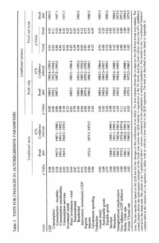
Table 3 TESTS FOR CHANGES IN AUTOREGRESSIVE PARAMETERS
Conditional variance
Conditional mean Break only Trend and break
67% 67% p-Value Break Confidence Break Confidence Break
Series p-Value date interval p-Value date interval Trend Break date
GDP 0.98 0.00 1983:2 1982:4-1985:3 0.63 0.00 1983:2
Consumption 0.55 0.00 1992:1 1991:3-1994:1 0.00 0.11 Consumption-durables 0.04 1987:3 1987:1-1988:1 0.00 1987:3 1987:2-1990:2 0.68 0.03 1987:3
Consumption-nondurables 0.00 1991:4 1991:2-1992:2 0.08 0.96 0.80
Consumption-services 0.00 1969:4 1969:2-1970:2 0.18 0.03 0.00 1971:3 Investment (total) 0.05 0.13 0.06 0.25
Fixed investment-total 0.69 0.01 1983:3 1983:1-1986:4 0.65 0.07 Nonresidential 0.47 0.70 0.69 0.60 Residential 0.10 0.00 1983:2 1983:1-1985:2 0.08 0.00 1983:2
A(inventory investment) /GDP 0.91 0.04 1988:1 1987:3-1992:2 0.00 0.10
Exports 0.09 0.00 1975:4 1975:2-1978:2 0.95 0.75
Imports 0.00 1972:4 1972:2-1973:2 0.00 1986:2 1986:1-1988:1 0.96 0.05 1986:2 Goverment spending 0.06 0.45 0.33 0.65
Production Goods (total) 0.92 0.00 1983:4 1983:2-1986:4 0.54 0.03 1983:3
Nondurable goods 0.09 0.00 1983:4 1983:3-1987:1 0.00 0.29 Durable goods 0.77 0.02 1985:2 1984:3-1989:1 0.33 0.02 1985:2
Services 0.00 1968:3 1968:1-1969:1 0.98 0.69 0.92 Structures 0.02 1991:3 1991:1-1992:1 0.02 1984:2 1983:4-1988:1 0.42 0.03 1984:2
Nonagricultural employment 0.03 1981:2 1980:4-1981:4 0.00 1983:2 1982:4-1985:3 0.00 0.02 1973:3 Price inflation (GDP deflator) 0.00 1973:2 1972:4-1973:4 0.11 0.00 0.00 1971:2
90-day T-bill rate 0.00 1981:1 1980:3-1981:3 0.01 1984:4 1984:2-1988:1 0.00 0.00 1984:4
10-year T-bond rate 0.02 1981:1 1980:3-1981:3 0.00 1979:3 1972:2-1980:1 0.02 0.00 1979:3
Notes: The test results are based on the QLR test for the changes in the coefficients of an AR(4). The first column shows the p-value for the QLR-test break test statistic. The second column shows the least-squares estimates of the break date (when the QLR statistic is significant at the 5% level), and the final column shows the 67% confidence interval for the break date. The results in the "Conditional Mean" columns correspond to the parameters a and i in equation (1). The results in the "Conditional Variance" columns refer to the variance of e, in equation (1), either with or without a time trend in the QLR regression. The tests are described in more detail in Appendix A.
Has the Business Cycle Changed and Why? ? 173
and Kim, Nelson, and Piger (2001). The 67% confidence interval for the break date is precise, 1982:4-1985:3, although (for reasons discussed in footnote 4) the 95% confidence interval is rather wide, 1982:1-1989:4.
The results for the components of GDP indicate that although several series (such as the components of consumption) reveal significant time variation in the conditional-mean coefficients, the estimated break dates and confidence intervals do not coincide with the timing of the reductions in volatility evident in Figure 2. In contrast, for ten of the seventeen NIPA
components there are significant changes in the conditional variance, and for eight of those ten series the break in the conditional variance is esti- mated to be in the mid-1980s. Thus, like Kim, Nelson, and Piger (2001), who use Bayesian methods, we find breaks in the volatility of many components of GDP, not just durable-goods output as suggested by McConnell and Perez-Quiros (2000). Durables consumption, total fixed investment, residential investment, imports, goods production, and em-
ployment all exhibit significant breaks in their conditional volatility with break dates estimated in the mid-1980s.
3.1.4 Estimates Based on the Stochastic Volatility Model As another check on this conclusion, we recalculated the estimates of the instantaneous variance based on the stochastic volatility model (the smooth lines in Fig- ure 2), with the restriction that the AR coefficients remain constant at their
full-sample OLS estimated values. The resulting estimated instantaneous standard deviations (not reported here) were visually very close to those
reported in Figure 2. The most substantial differences in the estimated instantaneous variance was for price inflation, in which changes in the conditional-mean coefficients in the 1960s contributed to changes in the estimated standard deviation. These results are consistent with the con- clusion drawn from Table 3 that the reduction in the variance of these series is attributable to a reduction in the conditional variance.
3.1.5 Resultsfor Other Series Results for additional time series are summa- rized in Table 10 in Appendix A. There is evidence of widespread instabil-
ity in both the conditional mean and the conditional variance. Half of the 168 series show breaks in their conditional-mean parameters [consistent with the evidence in Stock and Watson (1996)]. Strikingly, the hypothesis of a constant variance is rejected in two-thirds of the series. Sensier and van Dijk (2001) find a similar result in their analysis of 215 U.S. macroeco- nomic time series. The breaks in the conditional means are mainly concen- trated in the 1970s. In contrast, the breaks in the conditional variances are concentrated in the 1980s or, for some series, the early 1990s. Thus, the
timing of the reduction in the unconditional variance of these series in
174 . STOCK & WATSON
the 1980s and 1990s coincides with the estimated breaks in the conditional variance, not with the estimated breaks in the conditional means.
3.2 IS THE MODERATION A TREND OR A BREAK?
Kim and Nelson (1999) and McConnell and Perez-Quiros (2000) modeled the volatility reduction using Markov switching models; like the AR model (1) with coefficient breaks, the Markov switching model treats the moderation as a discrete event, which they independently dated as oc-
curring in 1984:1. After examining evidence on rolling standard deviations, however, Blanchard and Simon (2001) argued that the volatility reduc- tion was better viewed as part of a longer trend decline, in which the high volatility of the late 1970s and early 1980s was a temporary aberration.
To elucidate this trend-vs.-break debate, we conduct some additional tests using a model that nests the two hypotheses. Specifically, the QLR test for a change in the standard deviation in Section 3.1 was modified so that the model for the heteroscedasticity includes a time trend as well as the break. That is, the QLR test is based on the regression I tl = 70 +
Ylt + 72dt(T) + ilt, where dt(T) is a binary variable that equals 1 if t - T and equals zero otherwise, and rl, is an error term; the modified QLR test looks for breaks for values of T in the central 70% of the sample.
The results are reported in the final columns of Table 3. For GDP, the coefficient on the time trend is not statistically significantly different from zero, while the hypothesis of no break (maintaining the possibility of a time trend in the standard deviation) is rejected at the 1% significance level. The estimated break date in GDP volatility is 1983:2, the same whether a time trend is included in the specification or not. For GDP, then, this evidence is consistent with the inference drawn from the estimated instantaneous standard deviation plotted in Figure 2: the sharp decline in the volatility of GDP growth in the mid-1980s is better described as a discrete reduction in the variance than as part of a continuing trend to- wards lower volatility.
The results in Table 2 suggest that the break model is also appropriate for many of the components of GDP, specifically nondurables consump- tion, residential fixed investment, imports, total goods production, pro- duction of durables, and production of construction. For these series, the estimated break dates fall between 1983:2 and 1987:3. Consumption of durables and production of nondurables, however, seem to be better de- scribed by the trend model. A few of the components of GDP, such as
exports, are not well described by either model. These conclusions based on Table 2 are consistent with those based on
the smoothed volatility plots in Figure 2: there was a sharp decline, or
Has the Business Cycle Changed and Why? ? 175
break, in the volatility of GDP growth and some of its components, most
strikingly residential investment, durable-goods output, and output of construction, while other components and time series show more compli- cated patterns of time-varying volatility.
3.3 MULTIVARIATE ESTIMATES OF BREAK DATES
In theory, a common break date can be estimated much more precisely when multiple-equation methods are used [see Hansen (2001) for a re- view]. In this section, we therefore use two multivariate methods in an
attempt to refine the break-date confidence intervals of Section 3.1, one based on low-dimensional VARs, the other based on dynamic factor models.
3.3.1 Common Breaks in VARs To estimate common breaks across multi-
ple series, we follow Bai, Lumsdaine, and Stock (1998) and extend the univariate autoregression in (1) to a VAR. The procedure is the same as described in Section 3.1, except that, to avoid overfitting, the VAR coeffi- cients were kept constant. The hypothesis of no break is tested against the alternative of a common break in the system of equations using the QLR statistic computed using the absolute values of the VAR residuals. We also report the OLS estimator of the break date in the mean absolute residual and the associated 67% confidence interval, computed using the formulas in Bai, Lumsdaine, and Stock (1998).
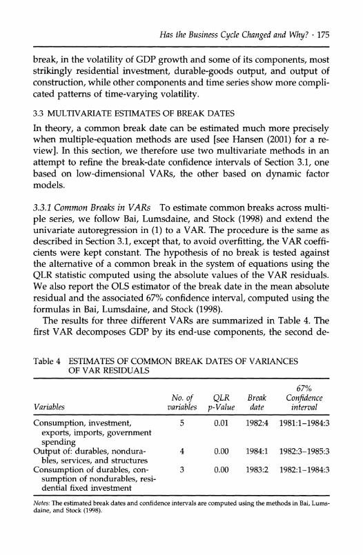
The results for three different VARs are summarized in Table 4. The first VAR decomposes GDP by its end-use components, the second de-
Table 4 ESTIMATES OF COMMON BREAK DATES OF VARIANCES OF VAR RESIDUALS
67% No. of QLR Break Confidence
Variables variables p-Value date interval
Consumption, investment, 5 0.01 1982:4 1981:1-1984:3 exports, imports, government spending
Output of: durables, nondura- 4 0.00 1984:1 1982:3-1985:3 bles, services, and structures
Consumption of durables, con- 3 0.00 1983:2 1982:1-1984:3 sumption of nondurables, resi- dential fixed investment
Notes: The estimated break dates and confidence intervals are computed using the methods in Bai, Lums- daine, and Stock (1998).
176 * STOCK & WATSON
composes GDP by its production components, and the third focuses on the more durable components of demand by individuals, consumption of nondurables and durables, and residential fixed investment. In each, the hypothesis of a constant variance is rejected at the 1% significance level. The estimated break dates range from 1982:4 to 1984:1, with 67% confidence intervals that are tight and similar to the 67% confidence inter- val based on the univariate analysis of GDP growth.
3.3.2 Evidence Based on Factor Models Dynamic factor models provide a
complementary way to use information on multiple variables to estimate the volatility break date. Chauvet and Potter (2001) use Bayesian methods to analyze a dynamic factor model of nine measures of economic activity (including GDP, industrial production, consumption, sales, and employ- ment). Their model allows for breaks in the autoregressive coefficients and variance of the single common dynamic factor. They find strong evidence for a break in the variance of the common factor, and the poste- rior distribution for the break date places almost all the mass in 1983 or 1984.
This analysis can be extended to higher-dimensional systems by using the principal components of the data to estimate the space spanned by the
postulated common dynamic factors (Stock and Watson, 2001). Previous
empirical work (Stock and Watson, 1999, 2001) has shown that the first
principal component computed using the series such as those in Appen- dix B captures a large fraction of the variation in those series, and that the first principal component can be thought of as a real activity factor. Like GDP, this factor has a significant break in its conditional variance, with an estimated break date of 1983:3 and a 67% confidence interval of 1983:2 to 1986:3.
3.4 SUMMARY
The results in this section point to instability both in conditional-mean functions and in conditional variances. The weight of the evidence, how- ever, suggests that the reductions in volatility evident in Table 1 and
Figure 2 are associated with changes in conditional variances (error vari- ances), rather than changes in conditional means (autoregressive coeffi- cients). Analysis of the full set of 168 series listed in Appendix B provides evidence of a widespread reduction in volatility, with the reduction gen- erally dated in the mid-1980s. For most series, this conclusion is un-
changed when one allows for the possibility that the volatility reduction could be part of a longer trend. Accordingly, we conclude that for most series the preferred model is one of a distinct reduction in volatility rather than a trend decline.
Has the Business Cycle Changed and Why? ? 177
This view of a sharp moderation rather than a trend decline is particu- larly appropriate for GDP and some of its more durable components. Fol-
lowing McConnell and Perez-Quiros (2000), much of the literature focuses on declines in volatility in the production of durable goods; however, like Kim, Nelson, and Piger (2001), we find significant reductions in volatility in other series. Our results particularly point to large reductions in the variance of residential fixed investment and output of structures, both of which are highly volatile. The finding of a break in volatility in the mid- 1980s is robust, and univariate and multivariate confidence intervals for the break date are tightly centered around 1983 and 1984.
4. Impulse or Propagation? The univariate analysis of Section 3.1 suggests that most of the moder- ation in volatility of GDP growth is associated with a reduction in its conditional variance, not changes in its conditional mean. But does this conclusion hold when multiple sources of information are used to com-
pute the conditional mean of output growth? Several recent studies (Ahmed, Levin, and Wilson 2001; Boivin and Giannoni, 2002a; 2002b; Primiceri (2002); Simon, 2000) have examined this question using vector
autoregressions, and we adopt this approach here. Specifically, in the con- text of reduced-form VARs, is the observed reduction in volatility associ- ated with a change in the magnitude of the VAR forecast errors (the impulses), in the lag dynamics modeled by the VAR (propagation), or both?
4.1 THE COUNTERFACTUAL VAR METHOD
Because the results of Sections 3.2 and 3.3 point to a distinct break in
volatility in 1983 or 1984, in this section we impose the break date 1984:1 found by Kim and Nelson (1999) and McConnell and Perez-Quiros (2000). Accordingly, we use reduced-form VARs estimated over 1960-1983 and 1984-2001 to estimate how much of the reduction in the variance of GDP is due to changes in the VAR coefficients and how much is due to changes in the innovation covariance matrix. Each VAR has the form
Xt = <i(L)Xt_- + ut, Var(u) = i,, (2)
where Xt is a vector time series and the subscript i = 1, 2 denotes the first and second subsample [the intercept is omitted in (2) for notational convenience but is included in the estimation]. Let Bij be the matrix of coefficients of the jth lag in the matrix lag polynomial Bi(L) = [I -
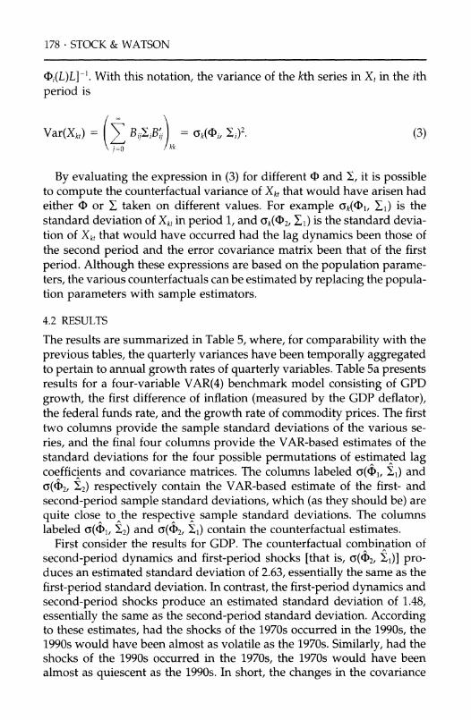
178 . STOCK & WATSON
4)i(L)L]-'. With this notation, the variance of the kth series in Xt in the ith period is
Var(Xkt) = B( j Bi,B =Ck(cI, ,)2. (3) j-Q kk
By evaluating the expression in (3) for different D and X, it is possible to compute the counterfactual variance of Xkt that would have arisen had either D or Z taken on different values. For example c(k(4)l, 1) is the standard deviation of Xkt in period 1, and ok(02, 1) is the standard devia- tion of Xkt that would have occurred had the lag dynamics been those of the second period and the error covariance matrix been that of the first
period. Although these expressions are based on the population parame- ters, the various counterfactuals can be estimated by replacing the popula- tion parameters with sample estimators.
4.2 RESULTS
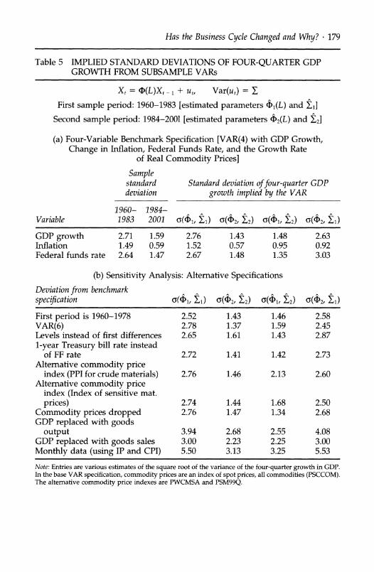
The results are summarized in Table 5, where, for comparability with the
previous tables, the quarterly variances have been temporally aggregated to pertain to annual growth rates of quarterly variables. Table 5a presents results for a four-variable VAR(4) benchmark model consisting of GPD
growth, the first difference of inflation (measured by the GDP deflator), the federal funds rate, and the growth rate of commodity prices. The first two columns provide the sample standard deviations of the various se- ries, and the final four columns provide the VAR-based estimates of the standard deviations for the four possible permutations of estimated lag coefficients and covariance matrices. The columns labeled c(01, Si) and C(42, / 2) respectively contain the VAR-based estimate of the first- and
second-period sample standard deviations, which (as they should be) are
quite close to the respective sample standard deviations. The columns labeled c(01,, 12) and ao(02, 1) contain the counterfactual estimates.
First consider the results for GDP. The counterfactual combination of
second-period dynamics and first-period shocks [that is, a(4)2, 1)] pro- duces an estimated standard deviation of 2.63, essentially the same as the
first-period standard deviation. In contrast, the first-period dynamics and
second-period shocks produce an estimated standard deviation of 1.48, essentially the same as the second-period standard deviation. According to these estimates, had the shocks of the 1970s occurred in the 1990s, the 1990s would have been almost as volatile as the 1970s. Similarly, had the shocks of the 1990s occurred in the 1970s, the 1970s would have been almost as quiescent as the 1990s. In short, the changes in the covariance
Has the Business Cycle Changed and Why? * 179
Table 5 IMPLIED STANDARD DEVIATIONS OF FOUR-QUARTER GDP GROWTH FROM SUBSAMPLE VARs
Xt = D(L)Xt -1 + Ut, Var(ut) = E
First sample period: 1960-1983 [estimated parameters 11(L) and El]
Second sample period: 1984-2001 [estimated parameters 42(L) and 2]
(a) Four-Variable Benchmark Specification [VAR(4) with GDP Growth, Change in Inflation, Federal Funds Rate, and the Growth Rate
of Real Commodity Prices]
Sample standard deviation
1960- 1984- 1983 2001 Variable
Standard deviation offour-quarter GDP growth implied by the VAR
(Ti2, ?1)
GDP growth 2.71 1.59 2.76 1.43 1.48 2.63 Inflation 1.49 0.59 1.52 0.57 0.95 0.92 Federal funds rate 2.64 1.47 2.67 1.48 1.35 3.03
(b) Sensitivity Analysis: Alternative Specifications Deviation from benchmark specification o(4i, 1) (62, 2) o(T, 12) (D2 X1)
First period is 1960-1978 2.52 1.43 1.46 2.58 VAR(6) 2.78 1.37 1.59 2.45 Levels instead of first differences 2.65 1.61 1.43 2.87 1-year Treasury bill rate instead
of FF rate 2.72 1.41 1.42 2.73 Alternative commodity price
index (PPI for crude materials) 2.76 1.46 2.13 2.60 Alternative commodity price
index (Index of sensitive mat. prices) 2.74 1.44 1.68 2.50
Commodity prices dropped 2.76 1.47 1.34 2.68 GDP replaced with goods
output 3.94 2.68 2.55 4.08 GDP replaced with goods sales 3.00 2.23 2.25 3.00 Monthly data (using IP and CPI) 5.50 3.13 3.25 5.53
Note: Entries are various estimates of the square root of the variance of the four-quarter growth in GDP. In the base VAR specification, commodity prices are an index of spot prices, all commodities (PSCCOM). The alternative commodity price indexes are PWCMSA and PSM99Q.
(Y(1, t) 0(62 2) ,( 1,),
180- STOCK & WATSON
matrix of the unforecastable components of the VARs-the impulses- account for virtually all of the reduction in the observed volatility of
output.
4.3 SENSITIVITY ANALYSIS AND COMPARISON WITH THE LITERATURE
The sensitivity of this finding to changes in the model specification or
assumptions is investigated in Table 5b. The conclusion from the bench- mark model-that it is impulses, not shocks, that are associated with the variance reduction-is robust to most changes reported in that table. For
example, similar results obtain when the first period is changed to end in 1978 (the second period remains 1984-2001); when log GDP, inflation, and the interest rate are used rather than their first differences; when
monthly data are used; and when GDP is replaced with goods output or sales. Dropping the commodity spot price index does not change the results, nor does using an alternative index of sensitive-materials prices [a smoothed version of which is used by Christiano, Eichenbaum, and Evans (1999)]. Curiously, however, replacing the commodity price index
by the produce price index for crude materials does change the conclu- sions somewhat, giving some role to propagation. The weight of this evi- dence, however, suggests that changes in the propagation mechanism
play at most a modest role in explaining the moderation of economic
activity. The substantive conclusions drawn from Table 5 are similar to Primi-
ceri's (2002), Simon's (2000), and (for the same sample periods) Boivin and Giannoni's (2002a, 2002b). Ahmed, Levin, and Wilson (2002) con- clude that most of the reduction in variance stems from smaller shocks, but give some weight to changes in the propagation mechanism. The main source of the difference between our results and theirs appears to be that Ahmed, Levin, and Wilson (2002) measure commodity prices by the pro- ducer price index for crude materials.
4.4 CONCLUSIONS
The estimates in Table 5 suggest that most, if not all, of the reductions in the variance of the four-quarter growth of GDP are attributable to changes in the covariance matrix of the reduced-form VAR innovations, not to changes in the VAR lag coefficients (the propagation mechanism). These changes in reduced-form VAR innovations could arise either from reduc- tions in the variance of certain structural shocks or from changes in how those shocks impact the economy, notably through changes in the struc- ture of monetary policy. To sort out these possibilities, however, we need
Has the Business Cycle Changed and Why? ? 181
to move beyond reduced-form data description and consider structural economic models, a task taken up in the next section.
5. Explanations for the Great Moderation What accounts for the moderation in the volatility of GDP growth and, more generally, for the empirical evidence documented in Sections 2-4? In this section, we consider five potential explanations. The first is that the reduction in volatility can be traced to a change in the sectoral com-
position of output away from durable goods. The second potential ex-
planation, proposed by McConnell and Perez-Quiros (2000), is that the reduction in volatility is due to new and better inventory management practices. The third possibility emphasizes the volatility reduction in resi- dential fixed investment. The fourth candidate explanation is that the structural shocks to the economy are smaller than they once were: we
simply have had good luck. Finally, we consider the possibility that the reduction in volatility is, at least in part, attributable to better macroeco- nomic policy, in particular better policymaking by the Federal Reserve Board.
5.1 CHANGES IN THE SECTORAL COMPOSITION
The service sector is less cyclically sensitive than the manufacturing sec- tor, so, as suggested by Burs (1960) and Moore and Zamowitz (1986), the shift in the United States from manufacturing to services should lead to a reduction in the variability of GDP. Blanchard and Simon (2001), McConnell and Perez-Quiros (2000), and Wamock and Wamock (2001) investigated this hypothesis and concluded that this sectoral shift hypoth- esis does not explain the reduction in volatility. The essence of Blanchard and Simon's (2001) and McConnell and Perez-Quiros's (2000) argument is summarized in Table 6a. The standard deviation of annual GDP growth fell from 2.7% during 1960-1983 to 1.6% during 1984-2001; when the out-
put subaggregates of durables, nondurables, services, and structures are combined using constant 1965 shares, the resulting standard deviations for the two periods are 3.1% and 1.8%. Thus, autonomously fixing the
output shares of the different sectors yields essentially the same decline in the standard deviation of GDP growth as using the actual, changing shares. Mechanically, the reason for this is that the volatility of output in the different sectors has declined across the board. Moreover, the sectors with the greatest volatility-durables and structures-also have output shares that are essentially constant.
The same result is evident if (like Warock and Warnock, 2001) one
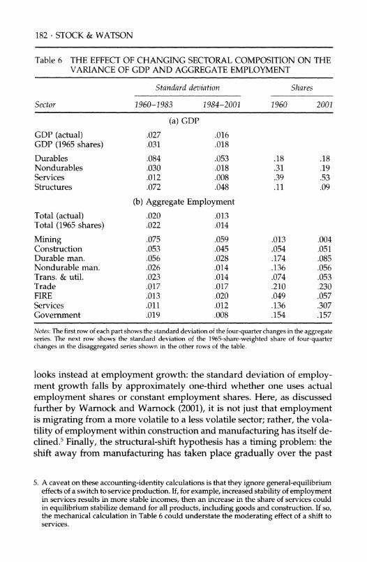
182 * STOCK & WATSON
Table 6 THE EFFECT OF CHANGING SECTORAL COMPOSITION ON THE VARIANCE OF GDP AND AGGREGATE EMPLOYMENT
Standard deviation Shares
Sector 1960-1983 1984-2001 1960 2001
(a) GDP
GDP (actual) .027 .016 GDP (1965 shares) .031 .018
Durables .084 .053 .18 .18 Nondurables .030 .018 .31 .19 Services .012 .008 .39 .53 Structures .072 .048 .11 .09
(b) Aggregate Employment Total (actual) .020 .013 Total (1965 shares) .022 .014
Mining .075 .059 .013 .004 Construction .053 .045 .054 .051 Durable man. .056 .028 .174 .085 Nondurable man. .026 .014 .136 .056 Trans. & util. .023 .014 .074 .053 Trade .017 .017 .210 .230 FIRE .013 .020 .049 .057 Services .011 .012 .136 .307 Government .019 .008 .154 .157
Notes: The first row of each part shows the standard deviation of the four-quarter changes in the aggregate series. The next row shows the standard deviation of the 1965-share-weighted share of four-quarter changes in the disaggregated series shown in the other rows of the table.
looks instead at employment growth: the standard deviation of employ- ment growth falls by approximately one-third whether one uses actual
employment shares or constant employment shares. Here, as discussed further by Warnock and Wamock (2001), it is not just that employment is migrating from a more volatile to a less volatile sector; rather, the vola-
tility of employment within construction and manufacturing has itself de- clined.5 Finally, the structural-shift hypothesis has a timing problem: the shift away from manufacturing has taken place gradually over the past
5. A caveat on these accounting-identity calculations is that they ignore general-equilibrium effects of a switch to service production. If, for example, increased stability of employment in services results in more stable incomes, then an increase in the share of services could in equilibrium stabilize demand for all products, including goods and construction. If so, the mechanical calculation in Table 6 could understate the moderating effect of a shift to services.
Has the Business Cycle Changed and Why? ? 183
four decades, whereas the analysis of Sections 2-4 suggests a sharp mod- eration in volatility in the mid-1980s.
5.2 CHANGES IN INVENTORY MANAGEMENT
McConnell and Perez-Quiros (2000) proposed that new inventory man-
agement methods, such as just-in-time inventory management, are the source of the reduction in volatility in GDP; this argument is elaborated
upon by Kahn, McConnell and Perez-Quiros (2001, 2002). The essence of their argument is that the volatility of production in manufacturing fell
sharply in the mid-1980s, but the volatility of sales did not; they found a
statistically significant break in output variability, especially in durables
manufacturing, but not in sales variability. They concluded that changes in inventory management must account for this discrepancy. Moreover, they suggested that the decline in the variance of goods production fully accounts for the statistical significance of the decline in GDP, so that un-
derstanding changes in inventory behavior holds the key to understand-
ing the moderation in GDP volatility. Unlike the sectoral-shift hypothesis, timing works in favor of this inventory-management hypothesis, for new
inventory management methods relying heavily on information technol-
ogy gained popularity during the 1980s. This bold conjecture-that micro-level changes in inventory manage-
ment could have major macroeconomic consequences-has received a
great deal of attention. Our reading of this research suggests, however, that upon closer inspection the inventory-management hypothesis does not fare well. The first set of difficulties pertain to the facts themselves. The stylized fact that production volatility has fallen but sales volatility has not is not robust to the method of analysis used or the series consid- ered. Ahmed, Levin, and Wilson (2002) find statistically significant evi- dence of a break in final sales in 1983:3 using the Bai-Perron (1998) test; Herrera and Pesavento (2002) use the QLR test and find a break in the variance of the growth of sales in nondurables manufacturing (estimated by least squares to be in 1983:3) and in durables manufacturing (in 1984: 1), as well as in many two-digit sectors; and Kim, Nelson, and Piger (2001) find evidence of a decline in volatility of aggregate final sales and in dura- ble goods sales using Bayesian methods.
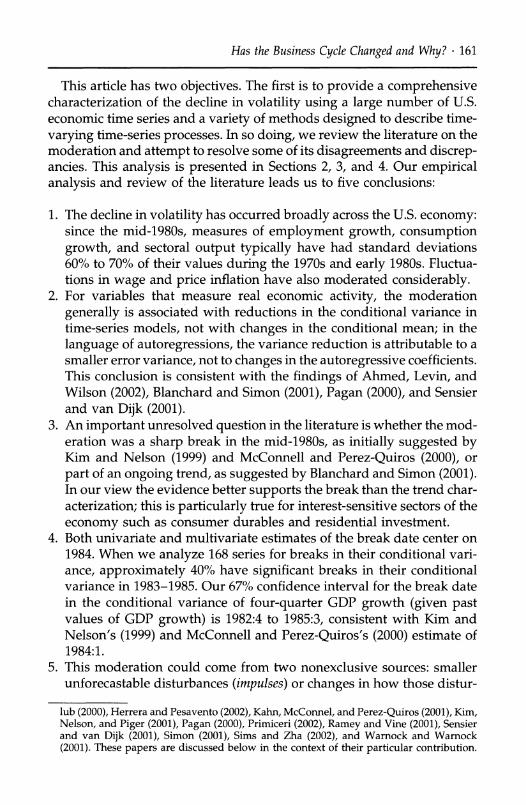
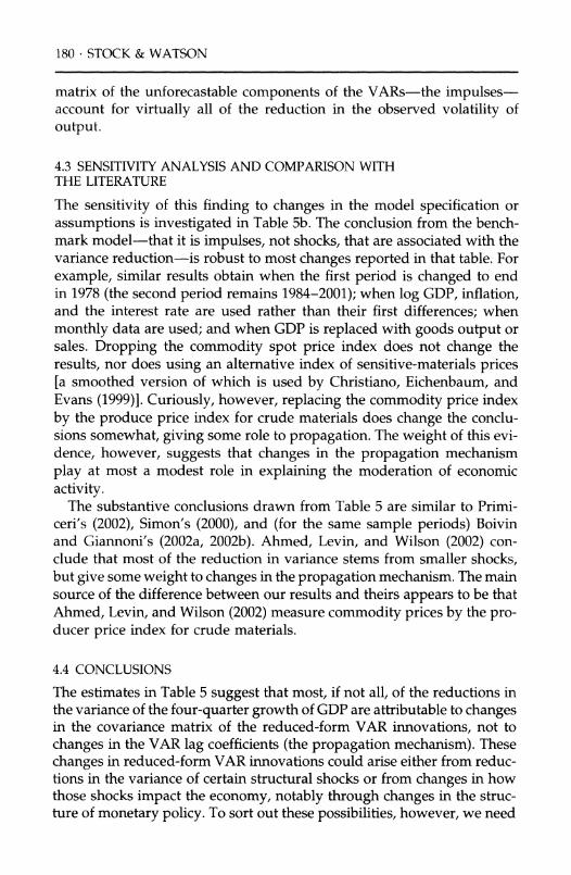
Our break-test results for sales (see Table 10) are consistent with this more recent literature: we find statistically significant breaks in the vari- ance of total final sales and final sales of durable goods. Like Kim, Nelson, and Piger (2001), we date the break in the variance of durable-goods sales to the early 1990s, whereas the break in the variance of production is dated to the mid-1980s. Although the confidence intervals for the break dates in durables production and sales are wide, the 67% confidence inter-
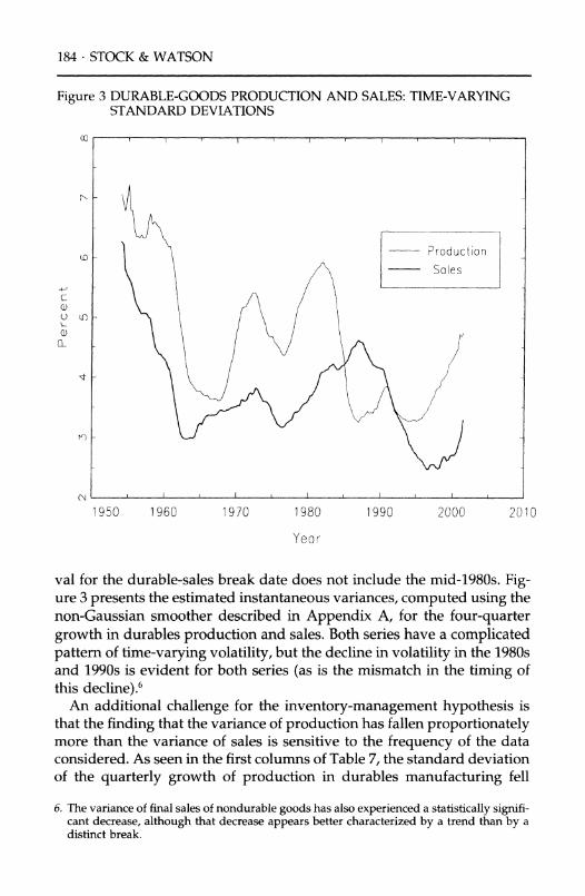
184 STOCK & WATSON
Figure 3 DURABLE-GOODS PRODUCTION AND SALES: TIME-VARYING STANDARD DEVIATIONS
- Production Sales
/I
r,
1950 1960 1970 1980 1990 2000 2010
Year
val for the durable-sales break date does not include the mid-1980s. Fig- ure 3 presents the estimated instantaneous variances, computed using the non-Gaussian smoother described in Appendix A, for the four-quarter growth in durables production and sales. Both series have a complicated pattern of time-varying volatility, but the decline in volatility in the 1980s and 1990s is evident for both series (as is the mismatch in the timing of this decline).6
An additional challenge for the inventory-management hypothesis is that the finding that the variance of production has fallen proportionately more than the variance of sales is sensitive to the frequency of the data considered. As seen in the first columns of Table 7, the standard deviation of the quarterly growth of production in durables manufacturing fell
6. The variance of final sales of nondurable goods has also experienced a statistically signifi- cant decrease, although that decrease appears better characterized by a trend than by a distinct break.
c 6)
-
._
I I I i i l l i l
( ... I
00
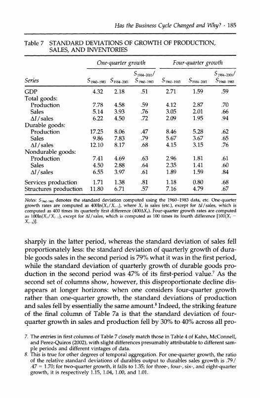
Has the Business Cycle Changed and Why? ? 185
Table 7 STANDARD DEVIATIONS OF GROWTH OF PRODUCTION, SALES, AND INVENTORIES
One-quarter growth Four-quarter growth
S1984-2001/ S1984-2001/ Series S 1960-1983 S 1984-2001 S 1960-1983 S 1960-1983 S 1984-2001 S 1960-1983
GDP 4.32 2.18 .51 2.71 1.59 .59 Total goods:
Production 7.78 4.58 .59 4.12 2.87 .70 Sales 5.14 3.93 .76 3.05 2.01 .66 AI / sales 6.22 4.50 .72 2.09 1.95 .94
Durable goods: Production 17.25 8.06 .47 8.46 5.28 .62 Sales 9.86 7.83 .79 5.67 3.67 .65 AI/sales 12.10 8.17 .68 4.15 3.15 .76
Nondurable goods: Production 7.41 4.69 .63 2.96 1.81 .61 Sales 4.50 2.88 .64 2.35 1.41 .60 AI/sales 6.55 3.97 .61 1.89 1.59 .84
Services production 1.71 1.38 .81 1.18 0.80 .68 Structures production 11.80 6.71 .57 7.16 4.79 .67
Notes: S1960-1983 denotes the standard deviation computed using the 1960-1983 data, etc. One-quarter growth rates are computed as 4001n(X,/X_ ), where X, is sales (etc.), except for AI/sales, which is computed as 400 times its quarterly first difference (400AX,). Four-quarter growth rates are computed as 1001n(X,/X, _), except for AI/sales, which is computed as 100 times its fourth difference [100(X, -
X,-4)].
sharply in the latter period, whereas the standard deviation of sales fell
proportionately less: the standard deviation of quarterly growth of dura- ble goods sales in the second period is 79% what it was in the first period, while the standard deviation of quarterly growth of durable goods pro- duction in the second period was 47% of its first-period value.7 As the second set of columns show, however, this disproportionate decline dis-
appears at longer horizons: when one considers four-quarter growth rather than one-quarter growth, the standard deviations of production and sales fell by essentially the same amount.8 Indeed, the striking feature of the final column of Table 7a is that the standard deviation of four-
quarter growth in sales and production fell by 30% to 40% across all pro-
7. The entries in first columns of Table 7 closely match those in Table 4 of Kahn, McConnell, and Perez-Quiros (2002), with slight differences presumably attributable to different sam- ple periods and different vintages of data.
8. This is true for other degrees of temporal aggregation. For one-quarter growth, the ratio of the relative standard deviations of durables output to durables sales growth is .79/ .47 = 1.70; for two-quarter growth, it falls to 1.35; for three-, four-, six-, and eight-quarter growth, it is respectively 1.15, 1.04, 1.00, and 1.01.
186 . STOCK & WATSON
duction sectors: durables, nondurables, services, and structures. This
suggests that, to the extent that information technology has facilitated
using inventories to smooth production, this effect is one of smoothing across months or across adjacent quarters. At the longer horizons of inter- est in business-cycle analysis, such as the four-quarter growth rates con- sidered in this paper, the declines in volatility of production and sales have been effectively proportional, suggesting no role for improved in-
ventory management in reducing volatility at longer horizons. The inventory-management hypothesis confronts other difficulties as
well. As emphasized by Blinder and Maccini (1991) and Ramey and West (1999), most inventories in manufacturing are raw materials or work-in-
progress inventories, which do not play a role in production smoothing (except avoiding raw-material stockouts). One would expect inventory- sales ratios to decline if information technology has an important impact on aggregate inventories; however, inventory-sales ratios have declined
primarily for raw materials and work-in-progress inventories, and in fact have risen for finished-goods inventories and for retail and wholesale trade inventories. Information technology may have improved the man-
agement of finished-goods inventories, but this improvement is not re- flected in a lower inventory-sales ratio for finished goods.
Ramey and Vine (2001) offer a different explanation of the relative de- cline in the variance of production at high frequencies, relative to sales.
They suggest that a modest reduction in the variance of sales can be mag- nified into a large reduction in the variance of production because of nonconvexities in plant-level cost functions. In their example, a small re- duction in the variance of auto sales means that sales fluctuations can be met through overtime rather than by (for example) adding temporary shifts, thereby sharply reducing the variance of output and employee- hours.
None of this evidence is decisive. Still, in our view it suggests that the reduction of volatility is too widespread across sectors and across produc- tion and sales (especially at longer horizons) to be consistent with the view that inventory management plays a central role in explaining the
economywide moderation in volatility.
5.3 RESIDENTIAL HOUSING
Although residential fixed investment constitutes a small share of GDP, historically it has been highly volatile and procyclical. The estimated in- stantaneous variance of the four-quarter growth in residential investment is 14.2 percentage points in 1981, but this falls to 6.0 percentage points in 1985. As is evident in Figure 2, even after weighting by its small share in GDP, the standard deviation fell during the mid-1980s by approximately
Has the Business Cycle Changed and Why? * 187
the same amount as did the share-weighted standard deviation of durable-
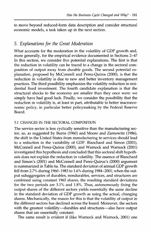
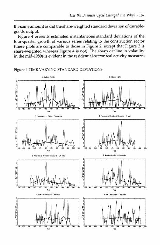
goods output. Figure 4 presents estimated instantaneous standard deviations of the
four-quarter growth of various series relating to the construction sector
(these plots are comparable to those in Figure 2, except that Figure 2 is
share-weighted whereas Figure 4 is not). The sharp decline in volatility in the mid-1980s is evident in the residential-sector real activity measures
Figure 4 TIME-VARYING STANDARD DEVIATIONS
A. Building Permits B. Housing Storts
Yeor Yeor
C. Ermpoyment -- Contract Construction D. Purchases of Residential Structures - I-unit
Year Year
E. Purchases of Residential Structures - 2+ units F. New Construction -- Residentiol
/ 1950 1955 1960 1965 1970 1975 1980 1985 1990 1995 2000 r
Year
G. New Construction -- Commercial
Io~~~ I
o
0 1
o1950 1955 1960 1965 1970 1975 1980 1985 1990 1995 2000 2005
Yeor
H. New Construction -- Industriol
I
e
o
e
aI
)5

188 . STOCK & WATSON
of building permits, housing starts, and real private residential construc- tion put in place. In contrast, nonresidential construction does not show
any volatility reduction: the variance of real industrial construction is ap- proximately constant, while the variance of real commercial construction is constant and then increases slightly during the 1990s. As noted by War- nock and Warock (2001), employment in total contract construction (which includes residential and nonresidential) also shows a decline in
volatility, although it is not as sharp as for the output measures. Intrigu- ingly, the decline in volatility of purchases of residential structures is more distinct for single-unit than for multiunit residences.
There are a variety of potential explanations for this marked decline in
volatility in the residential sector. One explanation emphasizes structural
changes in the market for home loans. As discussed in detail by McCarthy and Peach (2002), the mortgage market underwent substantial regulatory and institutional changes in the 1970s and 1980s. These changes included the introduction of adjustable-rate mortgages, the development of the sec-
ondary market for bundled mortgages, and the decline of thrifts and
growth of nonthrift lenders. To the extent that these changes reduced or eliminated credit rationing from the mortgage market, so that mortgages became generally available at the stated interest rate for qualified borrow- ers, they could have worked to reduce the volatility of demand for new
housing. According to this explanation, this autonomous decline in the
volatility of residential investment in turn spills over into a reduction of
volatility of aggregate demand. A difficulty with this explanation, how- ever, is that these institutional developments took time, and the drop in
volatility observed in Figure 4 is quite sharp. Moreover, McCarthy and Peach (2002) present evidence that although the impulse response of resi- dential investment to a monetary shock changed in the mid-1980s, the ultimate effect of a monetary shock on residential investment was essen-
tially unchanged; their results are, however, based on a Cholesky-factored VAR, and without a structural identification scheme they are hard to in-
terpret. Additional work is needed to ascertain if there is a relation be- tween the developments in the mortgage market and the stabilization of real activity in residential construction.9
9. U.S. financial markets generally, not just mortgage markets, developed substantially from the 1970s to 1990s. Blanchard and Simon (2001) suggest that increased consumer access to credit and equity ownership could have facilitated intertemporal smoothing of con- sumption, which in turn led to a reduction in aggregate volatility. Bekaert, Harvey, and Lundblad (2002) report empirical evidence based on international data that countries that liberalize equity markets experience a subsequent reduction in the volatility of economic growth. In the U.S., however, general financial market developments, like those in the mortgage market, took place over decades, whereas we estimate a sharp volatility reduc- tion in the mid-1980s: it seems the timing of the financial market developments in the U.S. does not match the timing of the reduction in volatility.
Has the Business Cycle Changed and Why? * 189
Other explanations suggest a more passive role for housing, that is, the reduction in housing volatility could be a response to the reduction in
general shocks to the economy. For example, if the decision to purchase a home is based in part on expected future income, and if expected future income is less volatile, then home investment should be less volatile. A
difficulty with this explanation is that, although the volatility of four-
quarter GDP growth has diminished, it is not clear that the volatility of
changes in permanent income has fallen. In fact, if there is a break in the variance of consumption of services, it is in the early 1970s and we do not find a statistically significant break in durables consumption (see Table 3). To the extent that nondurables consumption is a scaled measure of
permanent income, the variance of permanent income does not exhibit a
statistically significant break in the 1980s. This argument is quantified by Kim, Nelson, and Piger (2001), who in fact conclude that the reduction in the variance of GDP growth is associated with a decrease in the vari- ance of its cyclical, but not its long-run, component.
A related candidate explanation emphasizes the role of mortgage rates rather than expected incomes: the reduction in volatility of housing in- vestment reflects reduced volatility of expected real long-term rates. This is consistent with the reduction in the volatility of long and short interest rates in Figure 2, at least relative to the late 1970s and early 1980s. It is also consistent with the reduction in the volatility of durable-goods con-
sumption, sales, and production, which in part entail debt financing by consumers. To investigate this hypothesis, however, one would need to
develop measures of the expected variance of the ex ante real mortgage rate, to see how these measures changed during the 1980s, and to integrate this into a model of housing investment-topics that are left to future work.
5.4 SMALLER SHOCKS
The reduced-form VAR analysis of Section 4 suggested that most, possibly all, of the decline in the variance of real GDP growth is attributable to
changes in the covariance matrix of the VAR innovations. In this sec- tion, we attempt to pinpoint some specific structural shocks that have moderated. We consider five types of shocks: money shocks, fiscal shocks, productivity shocks, oil price shocks, and shocks to other commodity prices.
5.4.1 Money Shocks Over the past fifteen years, there has been consid- erable research devoted to identifying shocks to monetary policy and to measuring their effects on the macroeconomy. Two well-known ap- proaches, both using structural VARs but different identifying assump-

190 * STOCK & WATSON
tions, are Bemanke and Mihov (1998) (BM) and Christiano, Eichenbaum, and Evans (1997) (CEE) [see Christiano, Eichenbaum, and Evans (1999) for a survey]. Using structural VARs, we have implemented the BM and CEE identification strategies and computed the implied money shocks in the early (pre-1984) and late (post-1984) sample periods. Our specifica- tions are the same as used by those authors, although we extend their datasets.10 Bernanke and Mihov suggest that monetary policy shifted over the sample period, so we include a specification that incorporates this shift.
The standard deviation of the BM and CEE monetary shocks in the 1984-2001 sample period, relative to the standard deviation in the earlier
period, are reported in the first block of Table 8. Since the money shocks were very volatile during 1979-1983, results are shown for early sample periods that include and that exclude 1979-1983. The results suggest a marked decrease in the variability of monetary shocks for both CEE and BM identifications. The relative standard deviations over 1984-2001 are
roughly 0.50 when the early sample includes 1979-1983, and 0.75 when that period is excluded.
5.4.2 Fiscal Shocks Blanchard and Perotti (2001) identify shocks to taxes and government spending using a VAR together with an analysis of the automatic responses of these variables to changes in real income and in- flation. The next two rows of Table 8 show results for their shocks.1 There has been some moderation in both shocks; the standard deviation of tax shocks has fallen by approximately 20%.
5.4.3 Productivity Shocks Standard measures of productivity shocks, such as the Solow residual, suffer from measurement problems from variations in capacity utilization, imperfect competition, and other sources. While there have been important improvements in methods and models for
measuring productivity (for example, see Basu, Ferald, and Kimball, 1999), there does not seem to be a widely accepted series on productivity shocks suitable for our purposes. Instead we have relied on a method
suggested by Gali (1999) that, like the money and fiscal shocks, is based on a structural VAR. In particular, Gali associates productivity shocks with those components of the VAR that lead to permanent changes in
10. In our version of BM we use industrial production instead of their monthly interpolated GDP, because their series, and the related series in Bemanke, Gertler, and Watson (1997), end in 1997.
11. We thank Roberto Perotti for supplying us with the data and computer programs used to compute these shocks.
Has the Business Cycle Changed and Why? ? 191
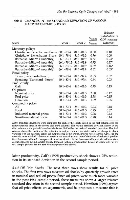
Table 8 CHANGES IN THE STANDARD DEVIATION OF VARIOUS MACROECONOMIC SHOCKS
Relative contribution to
perod2 GDP variance Shock Period 1 Period 2 Speriod 1 reduction
Monetary policy: Christiano-Eichenbaum-Evans 60:1-83:4 84:1-01:3 0.50 0.10 Christiano-Eichenbaum-Evans 60:1-78:4 84:1-01:3 0.76 0.00 Bemanke-Mihov-1 (monthly) 66:1-83:4 84:1-01:9 0.57 0.23* Bemanke-Mihov-1 (monthly) 66:1-78:12 84:1-01:9 0.75 0.27* Beranke-Mihov-2 (monthly) 66:1-83:12 84:1-01:9 0.39 0.16* Beranke-Mihov-2 (monthly) 66:1-78:4 84:1-01:9 0.62 0.05*
Fiscal policy: Taxes (Blanchard-Perotti) 60:1-83:4 84:1-97:4 0.83 0.02 Spending (Blanchard-Perotti) 60:1-83:4 84:1-97:4 0.94 0.03
Productivity: Gali 60:1-83:4 84:1-01:3 0.75 0.15
Oil prices: Nominal price 60:1-83:4 84:1-01:3 2.80 -0.12 Real price 60:1-83:4 84:1-01:3 2.98 -0.15 Hamilton 60:1-83:4 84:1-01:3 1.09 0.05
Commodity prices: All 60:1-83:4 84:1-01:3 0.73 0.18 Food 60:1-83:4 84:1-01:3 0.75 0.07 Industrial-material prices 60:1-83:4 84:1-01:3 0.78 0.13 Sensitive-material prices 60:1-83:4 84:1-01:3 0.78 0.14
Notes: Standard deviations were computed for each of the shocks listed in the first column over the sample periods listed in the second and third columns. The relative standard deviation shown in the third column is the period-2 standard deviation divided by the period-1 standard deviation. The final column shows the fraction of the reduction in output variance associated with the change in shock variance. For the quarterly series the output series is the annual growth rate of annual GDP. For the monthly series marked * the output series is the annual growth rate of the index of industrial produc- tion. Beranke-Mihov-1 corresponds to shocks estimated in the Bemanke-Mihov model with constant coefficients over the full sample period. Bemanke-Mihov-2 shocks allow the coefficients to differ in the two sample periods. See the text for description of the shocks.
labor productivity. Gali's (1999) productivity shock shows a 25% reduc- tion in its standard deviation in the second sample period.
5.4.4 Oil Price Shocks The next three rows show results for oil price shocks. The first two rows measure oil shocks by quarterly growth rates in nominal and real oil prices. Since oil prices were much more variable in the post-1984 sample period, these measures show a larger relative standard deviation in the second sample period. Hamilton (1996) argues that oil-price effects are asymmetric, and he proposes a measure that is
192 * STOCK & WATSON
the larger of zero and the percentage difference between the current price and the maximum price during the past year. Using Hamilton's measure, there has been essentially no change in the variability of oil shocks across the two sample periods.
5.4.5 Other Commodity Price Shocks The final four rows show results for broader commodity price measures: an aggregate index of commodity prices (the same measure often included in VAR models), an index for food, an index for industrial materials, and an index for sensitive materials. Results are shown for nominal growth rates (commodity price inflation); the results for real growth rates are essentially identical. These series show a marked reduction in volatility, with standard deviations falling between 20% and 30% in the second sample period relative to the first period.
5.4.6 Importance of These Reductions Whether the reductions in the vari- ances of the structural shocks can explain the moderation in GDP depends on the importance of these shocks in determining output growth. The final column of Table 8 reports the fraction of the reduction in the variance of four-quarter GDP growth that is explained by the change in the vari- ance of the shock in that row. For example, the reduction in the variance of the CEE monetary-policy shock explains 10% of the reduction in the variance of GDP growth when the first period ends in 1983 (but none of the reduction when the first period ends in 1978). The BM shock explains more of the reduction, at least in some specifications, although that per- centage reduction is not directly comparable to the other rows because it
pertains to industrial production. Fiscal-policy shocks make a negligible contribution, and oil price shocks either make a negligible contribution (the Hamilton shock) or go the wrong way, because oil price volatility increased in the second period. Productivity and commodity price shocks seem to have made modest contributions, in the neighborhood of 15%, to the reduction in the variance of four-quarter GDP growth.
It is tempting to add up the entries in the final column to produce a
composite number, but the result would be misleading. If these are true structural shocks, they should be uncorrelated with each other, but they are not; there is, in fact, considerable disagreement about whether these series are plausible proxies for the structural shocks they purport to esti- mate (e.g. Rudebusch, 1998). This said, although these shocks appear to
explain some of the observed reduction in the volatility, most-perhaps three-fourths-of the reduction in volatility is not explained by the reduc- tion in volatility of these shocks.
Has the Business Cycle Changed and Why? ? 193
5.5 CHANGES IN POLICY
An important candidate for the moderation in GDP growth is improved monetary policy.12 Most importantly, the timing is right: empirical studies
suggest that monetary policy changed significantly in the Volcker-
Greenspan era relative to earlier times. For example, Taylor (1999b), Clar- ida, Gali, and Gertler (2000), and Boivin and Giannoni (2002b) estimate
large increases in the inflation response in Taylor-type monetary policy rules for the short-term interest rate. Moreover, developments in financial markets are consistent with a shift in monetary policy. Although short rates are less variable than they were before 1984, they seem to be more
persistent: Watson (1999) reports that the (median unbiased) estimate of the largest AR root for monthly observations of the federal funds rate increased from 0.96 in the 1965-1978 sample period to 1.00 in the 1985- 1998 sample period.13 This increase in persistence has a large effect on the variance of expected future values of the federal funds rate, and hence on the expectations component of long-term rates. Indeed, while the vari- ance of short rates declined in the second sample period, the variance of
long rates, relative to that of short rates, increased. Taking this together with the evidence on changing Taylor-rule coefficients, it appears that the Fed has become more responsive to movements in inflation and out-
put and that these responses have led to increases in the variability of (medium- and long-term) interest rates.
There now are a number of studies examining the extent to which this
change in monetary policy-more precisely, this change in the rule ap- proximating monetary policy-caused the reduction of the variance of
output growth and/or inflation; see Boivin and Giannoni (2002a, 2002b), Clarida, Gali and Gertler (2000), Cogley and Sargent (2001), Gali, Lopez- Salido, and Valles (2002), Primiceri (2002), and Sims and Zha (2002). This is a challenging task: to evaluate the effect of a change in the monetary- policy rule, it is necessary to specify a model of the economy that is argu- ably invariant to the policy shift, that is, to specify a plausible structural model for the economy. The general strategy in this literature has been to combine some structural reasoning with VARs that permit the model to fit the dynamics in the data, but within this general framework the details of the approach differ widely. In this subsection, we perform these
12. As Taylor (2000) argues, fiscal policy is not a likely candidate. For example, Auerbach and Feenberg (2000) show that fiscal automatic stabilizers in 1995 were roughly at their same level as in the early 1960s, and if anything were higher in the late 1970s and early 1980s (because of high inflation and the lack of indexation of the tax code).
13. Similar results, obtained using different methods, are reported by Kim, Nelson, and Piger (2001) and Basistha and Startz (2001).
194 STOCK & WATSON
counterfactual policy evaluation calculations using a four-variable struc- tural VAR with GDP growth (y), GDP deflator inflation (n), the one-year Treasury bill rate (R), and commodity prices (PSCCOM, z).
5.5.1 Model Specification and Identification The structural VAR identifica- tion scheme is based on a structural model with an IS equation, a forward-
looking New Keynesian Phillips curve, a forward-looking Taylor-type monetary-policy rule, and an exogenous process for commodity prices:
yt = Ort + lags + Ey,t, (4)
it = yY(6)t + lags + ?,,t, (5)
rt = t ,Trlt+h/t + pyYl/t + lags + r,t, (6)
Zt = lags + oXyy,t + OCalT,t + CrEr,t + Ez,t, (7)
where rt = Rt - ft+k/t is the real interest rate; itt+k/t is the expected average inflation rate over the next k periods, where k is the term of the interest rate R; Y(6)t = 7r=o8'iy -/t is the discounted expected future output gap; and yia/t is the expected future average output gap over the next h pe- riods. We have used generic notation "lags" to denote unrestricted lags of variables in each of these equations.
Equation (4) is an IS relation. Equation (5) is a hybrid New Keynesian Phillips curve. If 8, the discount factor used to construct Y(6)t, is equal to 0, then this is a traditional formulation of the relation. More recent for- mulations based on price stickiness [discussed, for example, in Gali and Gertler (1999), Goodfriend and King (1997), and Rotemberg and Wood- ford (1997, 1999)] express Tt as a function of the output gap (as a proxy for marginal cost) and expected future inflation. Solving this equation forward yields (5) with 8 = 1. Allowing forward-looking and backward-
looking price setting yields (5) with 8 interpreted as the weight on for- ward inflation (Gali and Gertler, 1999). Equation (6) is a forward-looking Taylor rule, written in terms of the real interest rate. The parameter h indexes the horizon. For simplicity we use the same interest rate in (4) and (6), although in principle one would like to use long rates in (4) and short rates in (6).14 We use the 1-year interest rate as a compromise be- tween a long and short rate. Similarly, in our benchmark specification we use a 1-year horizon in (6), so that h = 4, but investigate the robustness of this as well. The commodity-price equation (7) plays no structural role
14. Both long and short rates could be included by adding a term structure equation as in Bemanke, Gertler, and Watson (1997).
Has the Business Cycle Changed and Why? ? 195
in the analysis, but, as is conventional, commodity prices are included to
help forecast future values of inflation and the output gap. As usual, the E's are taken to be mutually uncorrelated structural shocks.
5.5.2 Estimation Our estimation strategy relies on a priori knowledge of the three key parameters 0 (the slope of the IS function), y (the slope of the Phillips relation), and 6 (the parameter governing the forward-looking nature of the Phillips relation). Given these parameters, estimation pro- ceeds as follows. First, projecting all variables on lags produces a version of (4)-(7) in which the variables are replaced by reduced-form VAR re- siduals. (The forecasts of the output gap and inflation are computed by the VAR, so that innovations in these variables are also functions of the reduced-form VAR innovations.) We suppose that the forecast errors as- sociated with trend output are negligible, so we replace innovations in the expected future gap with innovations in expected future output. Then, with 0, 6 and y given, the errors cy and E? follow from (4) and (5). These errors are in turn used as instruments to estimate the parameters in the
Taylor rule, yielding ?r. The unknown coefficients in (7) can then be deter- mined by OLS. We assume that the parameters 0, 6, and y remain constant over the entire sample period, but we allow the parameter of the Taylor rule to change. We also allow the coefficients in equation (7) to change.
There is considerable disagreement about the values of the parameters 0, y, and 6 in the literature [see Rudebusch (2002)]. In our benchmark model, we set 0 = -0.2, y = 0.3, and 6 = 0.5. When simulating small
quantitative models, a larger value for 0 is sometimes used (e.g. 0 = -1), but large values of 0 are difficult to reconcile with IS slope estimates com-
puted by traditional methods (which often find values of 0 = - 0.1 or smaller). The value y = 0.3 was used by Clarida, Gali, and Gertler (2000) in their simulations of the effects of changes in monetary policy on output and inflation variability. Traditional estimates of the Phillips curve (for example, Staiger, Stock, and Watson, 2001) suggest values of y around 0.1. The value of 6 has also been the subject of controversy. Backward- looking models (such as Rudebusch, and Svensson 1999) set 6 = 0, Gali and Gertler (1999) estimate 6 to be approximately 0.6, and many models are simulated with 6 = 1.0.
Table 9 summarizes the results for these benchmark parameter values. Results are presented for the 1960-1978 and 1984-2001 sample periods. The estimated Taylor-rule coefficients (Table 9a) are consistent with what others have found. The inflation response in the first period is negative (remember that we specify the Taylor rule using the real interest rate), and the output coefficient is small. In the second period both the inflation and output coefficients are significantly higher.
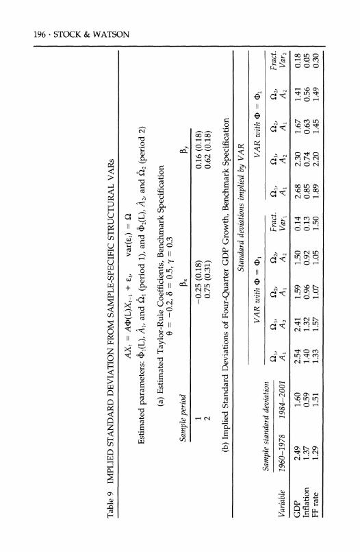
Table 9 IMPLIED STANDARD DEVIATION FROM SAMPLE-SPECIFIC STRUCTURAL VARs
AXt = Ad)(L)Xt,l + ?t, var(Et) =
Estimated parameters: li(L), Al, and Ql (period 1), and D2(L), A2, and Q2 (period 2)
(a) Estimated Taylor-Rule Coefficients, Benchmark Specification 0 = -0.2, 6 = 0.5, y = 0.3
Sample period P Py
1 -0.25 (0.18) 0.16 (0.18) 2 0.75 (0.31) 0.62 (0.18)
(b) Implied Standard Deviations of Four-Quarter GDP Growth, Benchmark Specification
Standard deviations implied by VAR
VAR with do = 4 l VAR with D = 4 2 Sample standard deviation
Ql, Ql, Q2, Q2, Fract. Ql, Ql, Q2, Q2, Fract. Variable 1960-1978 1984-2001 A1 A2 A1 A2 Varl A1 A2 A1 A2 Var2
GDP 2.49 1.60 2.54 2.41 1.59 1.50 0.14 2.68 2.30 1.67 1.41 0.18 Inflation 1.37 0.59 1.40 1.32 0.96 0.92 0.13 0.85 0.74 0.63 0.56 0.05 FF rate 1.29 1.51 1.33 1.57 1.07 1.05 1.50 1.89 2.20 1.45 1.49 0.30
'IC .D
R?
Z
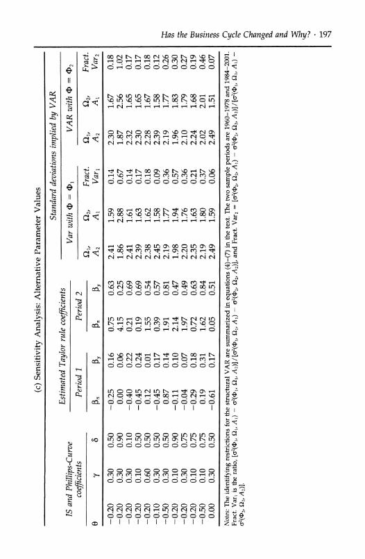
(c) Sensitivity Analysis: Alternative Parameter Values
Standard deviations implied by VAR Estimated Taylor rule coefficients
IS and Phillips-Curve , Var with (f = - VAR with 4i -= (2 coefficients Period 1 Period 2
Q , QPP2, Fract. 12 , Q2, Fract. 0 Y 6 P Py P Pay A2 A1 Varl A2 A1 Var2
-0.20 0.30 0.50 -0.25 0.16 0.75 0.63 2.41 1.59 -0.20 0.30 0.90 0.00 0.06 4.15 0.25 1.86 2.88 -0.20 0.30 0.10 -0.40 0.22 0.21 0.69 2.41 1.61 -0.20 0.10 0.50 -0.45 0.24 0.19 0.69 2.39 1.63 -0.20 0.60 0.50 0.12 0.01 1.55 0.54 2.38 1.62 -0.10 0.30 0.50 -0.45 0.17 0.39 0.57 2.45 1.58 -0.50 0.30 0.50 0.87 0.14 1.91 0.81 2.19 1.77 -0.20 0.10 0.90 -0.11 0.10 2.14 0.47 1.98 1.94 -0.20 0.30 0.75 -0.04 0.07 1.97 0.49 2.20 1.76 -0.20 0.10 0.75 -0.29 0.18 0.72 0.63 2.35 1.63 -0.50 0.10 0.75 0.19 0.31 1.62 0.84 2.19 1.80
0.00 0.30 0.50 -0.61 0.17 0.05 0.51 2.49 1.59
0.14 2.30 1.67 0.67 1.87 2.56 0.14 2.32 1.65 0.17 2.30 1.65 0.18 2.28 1.67 0.09 2.39 1.58 0.36 2.19 1.77 0.57 1.96 1.83 0.36 2.10 1.79 0.21 2.24 1.68 0.37 2.02 2.01 0.06 2.49 1.51
Notes: The identifying restrictions for the structural VAR are summarized in equations (4)-(7) in the text. The two sample periods are 1960-1978 and 1984-2001. Fract. Var, is the ratio, [a2(1I, Qi, A1) - a2(l, lQ1, A2)]/[2(1, i, Q1, A,) - o2(f2, 22, A2)], and Fract. Var2 = [a2(c2, Q2, Al) - 2((D2, Q2, A2)]/[(y2((,, il, Al) - O2(cD2, l2, A2)].
rl+
;Z m
vZ
;t
;t
tn
143 r3 m
0.18 1.02 0.17 0.17 0.18 0.12 0.26 0.30 0.27 0.19 0.46 0.07
198 STOCK & WATSON
Armed with these estimated parameters, we can use the structural VAR to compute the implied variability of output growth, changes in inflation, and interest rates. The calculations are analogous to those carried in Sec- tion 4, except now the VAR is characterized by three sets of parameters: (4, the VAR distributed lag coefficients (just as in Section 4); ?Q, the covariance matrix of the structural shocks (?y, Ec, ?r, z); and A, the structural coeffi- cients (0, y, 6, [3, 3y, ocy, oc, ra) that link the structural and reduced form errors. We present results for the triples a(;i, Qi, Ak), for i, j, k = 1, 2
corresponding to the two sample periods. The results are shown in Table 9b. Using (lI, 2i, A1), the standard
deviation of the four-quarter growth rate of GDP is 2.54%. Using (42, Q2,
A2), the corresponding value is 1.41%. These are close to the estimates of the standard deviation of output growth computed directly from the sam-
ple moments of GDP. How much of this change in the variability of out-
put can be attributed to shocks (Q), and how much to policy (A)? The standard deviation of output using ((1, Q2, A1) is 1.59; using (01, Ql, A2), it is 2.41. These results suggest that 14% of the decrease in variance in output growth is associated with changes in the monetary-policy coefficients.l5 Said differently, most of the reduction in variability in output stems from smaller shocks, not from changes in the monetary-policy coefficients.
The results for other sets of parameter values are shown in Table 9c. To save space, this table only reports the estimated Taylor-rule coefficients for each subsample and the implied variability of output growth for the four counterfactual simulations. Looking across these results, the esti- mated effect of the change in monetary policy is larger when the IS curve is more elastic (0 is more negative), when the output gap receives more
weight in the Phillips curve (y is larger), and when the New Keynesian Phillips curve is more forward looking (5 is larger).
One notable special case is when 0 = 0, so that monetary policy has no effect on output growth within the period; this corresponds to a common
VAR-identifying restriction [see the discussion in Christiano, Eichen- baum, and Evans (1999)]. This assumption implies that the change in
monetary policy had little to do with the decline in output growth volatil-
ity (the estimated contribution to the variance reduction when 0 = 0, y =
0.3, and 6 = 0.5 is approximately 6%). For most of the parameter combina- tions examined in Table 9c, however, the estimated contribution of the
change in monetary policy to the reduction in the variance of four-quarter GDP growth falls in the range of 10% to 25%. Estimates with very large contributions are associated with implausibly large coefficients on infla-
15. The total decrease in the variance of output estimated using the VAR is 2.542 - 1.412. The estimated decrease associated with the change in A is 2.542 - 2.412. The ratio is 0.14.
Has the Business Cycle Changed and Why? * 199
tion in the estimated second-period Taylor rule (inflation responses of 4 or more).
5.5.3 Other Sensitivity Checks We performed a number of other sensitivity checks. These included reducing the horizon in the Taylor rule to one quarter; dropping the commodity price index from the VAR; replacing the commodity price index with the estimated first factor (principal com- ponent) constructed from the series listed in Appendix B [as suggested by Bemanke and Boivin's (2000) factor-augmented VARs]; and carrying out the counterfactuals holding the parameters a fixed at their period-1 values. The results from these models are similar to results from the speci- fications reported in Table 9 and, to save space, are not reported.
5.5.4 Summary Even within the stylized model of equations (4)-(7), there is considerable uncertainty about whether the widely perceived shift in monetary policy in the 1980s produced the moderation of output vola- tility. For the benchmark parameter values, and for other values that produce estimates of monetary reaction functions consistent with those discussed elsewhere in the literature, our calculations attribute perhaps 10% to 25% of the reduction in the variance of four-quarter GDP growth to improved monetary policy.
6. Conclusions and Remaining Questions There is strong evidence of a decline in the volatility of economic activity, both as measured by broad aggregates and as measured by a wide variety of other series that track specific facets of economic activity. For real GDP growth, the decline is, we think, best characterized as a sharp drop in the mid-1980s. This sharp decline, or break, in the volatility in real GDP growth is mirrored by declines in the variance of the four-quarter growth rates of consumption and production of durable goods, in residential fixed investment, and in the production of structures. Not all series, how- ever, have exhibited this sharp drop in volatility, and for some series the decline in their variance is better characterized as a trend or, possibly, an episodic return to the relative quiescence of the 1960s.
Our search for the causes of this great moderation has not been com- pletely successful, nor does one find a compelling case in the literature for a single cause. On the positive side, we find some role for improved monetary policy; our estimates suggest that the Fed's more aggressive response to inflation since the mid-1980s has contributed perhaps 10% to 25% of the decline in output volatility. In addition, we find some role for identifiable shocks, such as less volatile productivity shocks and commod-
200 . STOCK & WATSON
ity price shocks, in reducing the variance of output growth. But this leaves
much-perhaps half-of the decline in volatility unaccounted for. The shift away from manufacturing and towards services does not seem to
explain the moderation; nor do improvements in inventory management arising from information technology seem to us to be a source of the re- ductions in volatility of four-quarter GDP growth, although improved inventory management could help to smooth production within the month or quarter. Our reduced-form evidence suggests that this reduc- tion in volatility is associated with an increase in the precision of forecasts of output growth (and of other macroeconomic variables), but to a consid- erable extent we have not identified the specific source of the reduced forecast errors.
These results provide some clues for future work. Among the compo- nents of GDP, the clearest concomitant declines appear in durable goods (both consumption and production), in output of structures, and in residen- tial investment. The declines in volatility appear in a variety of measures of residential (but not nonresidential) construction, and further investiga- tion of the role of the housing sector in the moderation is warranted.
To the extent that improved policy gets some of the credit, then one can
expect at least some of the moderation to continue as long as the policy regime is maintained. But because most of the reduction seems to be due to good luck in the form of smaller economic disturbances, we are left with the unsettling conclusion that the quiescence of the past fifteen years could well be a hiatus before a return to more turbulent economic times.
Appendix A. Time-Series Methods This appendix describes the stochastic volatility model used to compute the smoothed estimates in Figures 2-4 and the variance-break tests in Tables 3 and 10.
A.1 STOCHASTIC VOLATILITY MODEL
The smoothed instantaneous standard deviations were estimated using a stochastic volatility model with time-varying autoregressive coefficients.
Specifically, let yt follow the time-varying AR process
p
yt = jtyt-j + GtEt,
j=l
(jt = Ojt-i + CjTjt,
In Io = In (t_ - + t,t
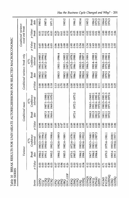
Table 10 BREAK RESULTS FOR UNIVARIATE AUTOREGRESSIONS FOR SELECTED MACROECONOMIC TIME SERIES
Conditional variance: Variance Conditional mean Conditional variance: break only trend and break
67% 67% 67% Break Confidence Break Confidence Break Confidence p-Value: p-Value: Break
Series p-Value date interval p-Value date interval p-Value date interval trend break date
GDPQ 0.00 1984:2 1983:3-1987:1 0.98 0.00 1983:2 1982:4-1985:3 0.65 0.00 1983:2 GCQ 0.00 1993:1 1992:3-1996:2 0.55 0.00 1992:1 1991:3-1994:1 0.00 0.12 GCDQ 0.00 1991:1 1990:4-1994:1 0.04 1987:3 1987:1-1988:1 0.00 1987:3 1987:2-1990:2 0.69 0.02 1987:3 GCNQ 0.38 0.00 1991:4 1991:2-1992:2 0.08 0.96 0.79 GCSQ 0.03 1993:2 1992:2-1998:4 0.00 1969:4 1969:2-1970:2 0.18 0.03 0.00 1971.3
GPIQ 0.07 0.05 0.13 0.06 0.26 GIFQ 0.02 1984:2 1982:4-1989:3 0.69 0.01 1983:3 1983:1-1986:4 0.66 0.07 GINQ 0.84 0.47 0.70 0.69 0.61 GIRQ 0.01 1983:3 1982:4-1989:1 0.10 0.00 1983:2 1983:1-1985:2 0.08 0.00 1983:2 DGV_GDP 0.26 0.91 0.04 1988:1 1987:3-1992:2 0.00 0.10
GEXQ 0.03 1973:1 1972:4-1978:1 0.09 0.00 1975:4 1975:2-1978:2 0.95 0.75 GIMQ 0.00 1985:3 1985:1-1990:2 0.00 1972:4 1972:2-1973:2 0.00 1986:2 1986:1-1988:1 0.96 0.05 1986.2 GGEQ 0.65 0.06 0.45 0.33 0.66 GOQ 0.01 1984:2 1983:2-1989:3 0.92 0.00 1983:4 1983:2-1986:4 0.54 0.02 1983:4 GODQ 0.04 1984:1 1983:4-1992:2 0.09 0.00 1983:4 1983:3-1987:1 0.00 0.30
GONQX 0.12 0.77 0.02 1985:2 1984:3-1989:1 0.34 0.02 1985:2 GOOSQ 0.00 1967:1 1965:3-1968:1 0.00 1968:3 1968:1-1969:1 0.98 0.69 0.93 GOCQ 0.01 1984:2 1983:1-1988:3 0.02 1991:3 1991:1-1992:1 0.02 1984:2 1983:4-1988:1 0.43 0.03 1984.2 LPNAG 0.03 1984:4 1981:1-1987:3 0.03 1981:2 1980:4-1981:4 0.00 1983:2 1982:4-1985:3 0.00 0.01 1973:3 GDPD 0.37 0.00 1973:2 1972:4-1973:4 0.11 0.00 0.00 1971:2
FYGM3 0.71 0.00 1981:1 1980:3-1981:3 0.01 1984:4 1984:2-1988:1 0.00 0.00 1984:4 FYGT10 0.01 1979:3 1975:4-1981:1 0.02 1981:1 1980:3-1981:3 0.00 1979:3 1972:2-1980:1 0.02 0.00 1979:3 GGFENQ 0.49 0.00 1972:2 1971:4-1972:4 0.00 1987:4 1984:2-1989:4 0.00 0.04 1974:3 GOSQ 0.03 1993:4 1993:2-2000:1 0.50 0.39 0.10 0.21 GODSQ 0.00 1991:1 1990:4-1997:1 0.06 0.05 0.55 0.06
co 'z-
to
;I
C)
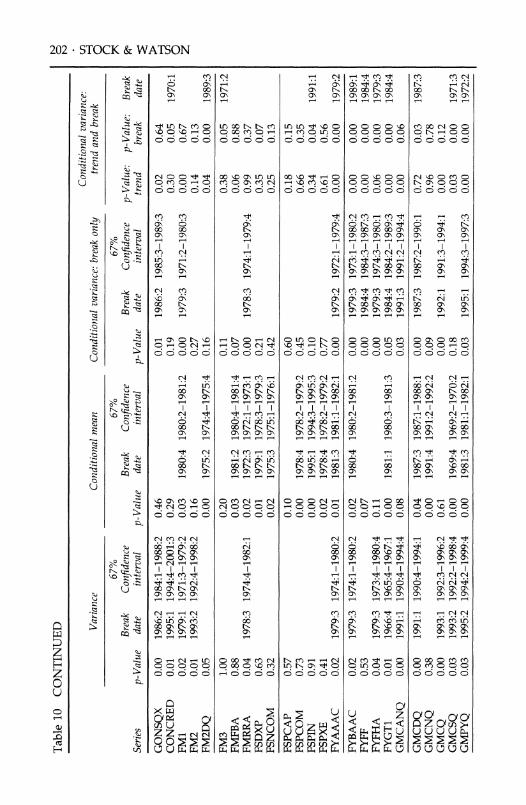
Table 10 CONTINUED
Conditional variance: Variance Conditional mean Conditional variance: break only trend and break
67% 67% 67% Break Confidence Break Confidence Break Confidence p-Value: p-Value: Break
Series p-Value date interval p-Value date interval p-Value date interval trend break date
GONSQX 0.00 1986:2 1984:1-1988:2 0.46 0.01 1986:2 1985:3-1989:3 0.02 0.64 CONCRED 0.01 1995:1 1994:4-2001:3 0.29 0.19 0.30 0.05 1970:1 FM1 0.02 1979:1 1971:3-1979:2 0.03 1980:4 1980:2-1981:2 0.00 1979:3 1971:2-1980:3 0.00 0.67 FM2 0.01 1993:2 1992:4-1998:2 0.16 0.27 0.14 0.13 FM2DQ 0.05 0.00 1975:2 1974:4-1975:4 0.16 0.04 0.00 1989:3
FM3 1.00 0.20 0.11 0.38 0.05 1971:2 FMFBA 0.88 0.03 1981:2 1980:4-1981:4 0.07 0.06 0.88 FMRRA 0.04 1978:3 1974:4-1982:1 0.02 1972:3 1972:1-1973:1 0.00 1978:3 1974:1-1979:4 0.99 0.37 FSDXP 0.63 0.01 1979:1 1978:3-1979:3 0.21 0.35 0.07 FSNCOM 0.32 0.02 1975:3 1975:1-1976:1 0.42 0.25 0.13
FSPCAP 0.57 0.10 0.60 0.18 0.15 FSPCOM 0.73 0.00 1978:4 1978:2-1979:2 0.45 0.66 0.35 FSPIN 0.91 0.00 1995:1 1994:3-1995:3 0.10 0.34 0.04 1991:1 FSPXE 0.41 0.02 1978:4 1978:2-1979:2 0.77 0.61 0.56 FYAAAC 0.02 1979:3 1974:1-1980:2 0.01 1981:3 1981:1-1982:1 0.00 1979:2 1972:1-1979:4 0.00 0.00 1979:2
FYBAAC 0.02 1979:3 1974:1-1980:2 0.02 1980:4 1980:2-1981:2 0.00 1979:3 1973:1-1980:2 0.00 0.00 1989:1 FYFF 0.53 0.07 0.00 1984:4 1984:3-1987:3 0.00 0.00 1984:4 FYFHA 0.04 1979:3 1973:4-1980:4 0.11 0.00 1979:3 1974:3-1980:1 0.06 0.00 1979:3 FYGT1 0.01 1966:4 1965:4-1967:1 0.00 1981:1 1980:3-1981:3 0.05 1984:4 1984:2-1989:3 0.00 0.00 1984:4 GMCANQ 0.00 1991:1 1990:4-1994:4 0.08 0.03 1991:3 1991:2-1994:4 0.00 0.06
GMCDQ 0.00 1991:1 1990:4-1994:1 0.04 1987:3 1987:1-1988:1 0.00 1987:3 1987:2-1990:1 0.72 0.03 1987:3 GMCNQ 0.38 0.00 1991:4 1991:2-1992:2 0.09 0.96 0.78 GMCQ 0.00 1993:1 1992:3-1996:2 0.61 0.00 1992:1 1991:3-1994:1 0.00 0.12 GMCSQ 0.03 1993:2 1992:2-1998:4 0.00 1969:4 1969:2-1970:2 0.18 0.03 0.00 1971:3 GMPYQ 0.03 1995:2 1994:2-1999:4 0.00 1981:3 1981:1-1982:1 0.03 1995:1 1994:3-1997:3 0.00 0.00 1972:2
tC
(f1 H
-z
z
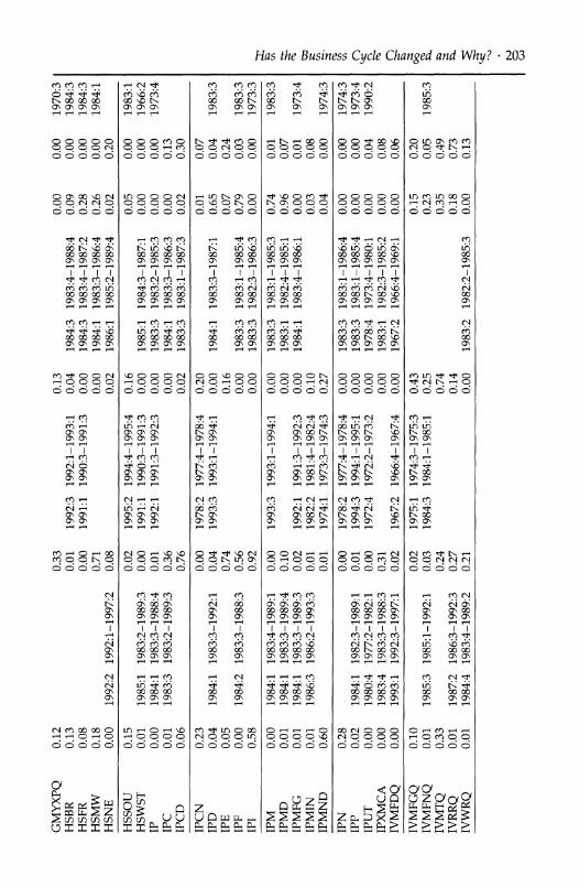
0.12 0.33 0.13 0.01 0.08 0.00 0.18 0.71 0.00 1992:2 1992:1-1997:2 0.08
0.13 1992:3 1992:1-1993:1 0.04 1984:3 1983:4-1988:4 1991:1 1990:3-1991:3 0.00 1984:3 1983:4-1987:2
0.00 1984:1 1983:3-1986:4 0.02 1986:1 1985:2-1989:4
HSSOU 0.15 0.02 1995:2 1994:4-1995:4 0.16 0.05 0.00 1983:1 HSWST 0.01 1985:1 1983:2-1989:3 0.00 1991:1 1990:3-1991:3 0.00 1985:1 1984:3-1987:1 0.00 0.00 1966:2 IP 0.00 1984:1 1983:3-1988:4 0.01 1992:1 1991:3-1992:3 0.00 1983:3 1983:2-1985:3 0.00 0.00 1973:4 IPC 0.01 1983:3 1983:2-1989:3 0.36 0.00 1984:1 1983:3-1986:3 0.00 0.13 IPCD 0.06 0.76 0.02 1983:3 1983:1-1987:3 0.02 0.30
IPCN 0.23 0.00 1978:2 1977:4-1978:4 0.20 0.01 0.07 IPD 0.04 1984:1 1983:3-1992:1 0.04 1993:3 1993:1-1994:1 0.00 1984:1 1983:3-1987:1 0.65 0.04 1983:3 IPE 0.05 0.74 0.16 0.07 0.24 IPF 0.00 1984:2 1983:3-1988:3 0.56 0.00 1983:3 1983:1-1985:4 0.79 0.03 1983:3 IPI 0.58 0.92 0.00 1983:3 1982:3-1986:3 0.00 0.00 1973:3
IPM 0.00 1984:1 1983:4-1989:1 0.00 1993:3 1993:1-1994:1 0.00 1983:3 1983:1-1985:3 0.74 0.01 1983:3 IPMD 0.01 1984:1 1983:3-1989:4 0.10 0.00 1983:1 1982:4-1985:1 0.96 0.07 IPMFG 0.01 1984:1 1983:3-1989:3 0.02 1992:1 1991:3-1992:3 0.00 1984:1 1983:4-1986:1 0.00 0.01 1973:4 IPMIN 0.01 1986:3 1986:2-1993:3 0.01 1982:2 1981:4-1982:4 0.10 0.03 0.08 IPMND 0.60 0.01 1974:1 1973:3-1974:3 0.27 0.04 0.00 1974:3
IPN 0.28 0.00 1978:2 1977:4-1978:4 0.00 1983:3 1983:1-1986:4 0.00 0.00 1974:3 IPP 0.02 1984:1 1982:3-1989:1 0.01 1994:3 1994:1-1995:1 0.00 1983:3 1983:1-1985:4 0.00 0.00 1973:4 IPUT 0.00 1980:4 1977:2-1982:1 0.00 1972:4 1972:2-1973:2 0.00 1978:4 1973:4-1980:1 0.00 0.04 1990:2 IPXMCA 0.00 1983:4 1983:3-1988:3 0.31 0.00 1983:1 1982:3-1985:2 0.00 0.08 IVMFDQ 0.00 1993:1 1992:3-1997:1 0.02 1967:2 1966:4-1967:4 0.00 1967:2 1966:4-1969:1 0.00 0.06
IVMFGQ 0.10 0.02 1975:1 1974:3-1975:3 0.43 0.15 0.20 IVMFNQ 0.01 1985:3 1985:1-1992:1 0.03 1984:3 1984:1-1985:1 0.25 0.23 0.05 1985:3 IVMTQ 0.33 0.24 0.74 0.35 0.49 IVRRQ 0.01 1987:2 1986:3-1992:3 0.27 0.14 0.18 0.73 IVWRQ 0.01 1984:4 1983:4-1989:2 0.21 0.00 1983:2 1982:2-1985:3 0.00 0.13
v)
cr
?-
t Nl3
GMYXPQ HSBR HSFR HSMW HSNE
0.00 0.09 0.28 0.26 0.02
0.00 1970:3 0.00 1984:3 0.00 1984:3 0.00 1984:1 0.20
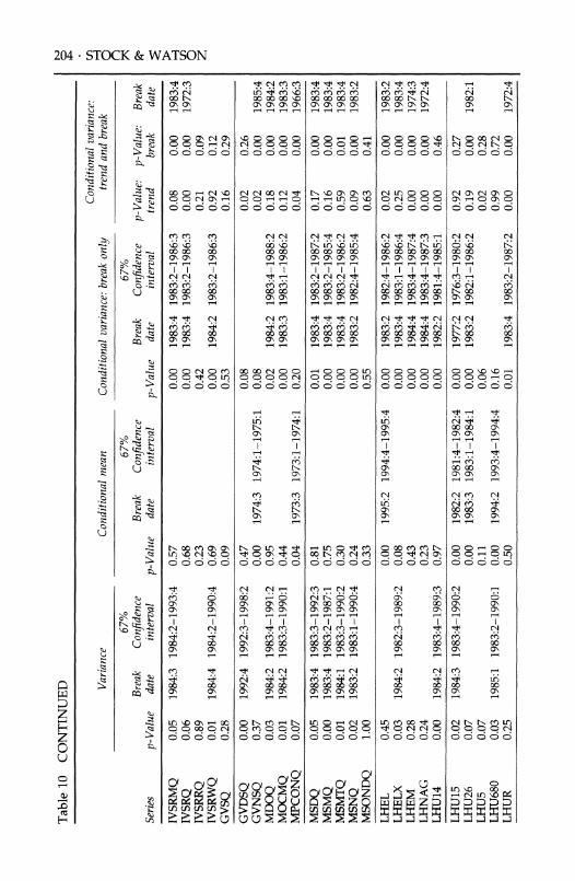
Table 10 CONTINUED
Conditional variance: Variance Conditional mean Conditional variance: break only trend and break
67% 67% 67% Break Confidence Break Confidence Break Confidence p-Value: p-Value: Break
Series p-Value date interval p-Value date interval p-Value date interval trend break date
IVSRMQ 0.05 1984:3 1984:2-1993:4 0.57 0.00 1983:4 1983:2-1986:3 0.08 0.00 1983:4 IVSRQ 0.06 0.68 0.00 1983:4 1983:2-1986:3 0.00 0.00 1972:3 IVSRRQ 0.89 0.23 0.42 0.21 0.09 IVSRWQ 0.01 1984:4 1984:2-1990:4 0.69 0.00 1984:2 1983:2-1986:3 0.92 0.12 GVSQ 0.28 0.09 0.53 0.16 0.29
GVDSQ 0.00 1992:4 1992:3-1998:2 0.47 0.08 0.02 0.26 GVNSQ 0.37 0.00 1974:3 1974:1-1975:1 0.08 0.02 0.00 1985:4 MDOQ 0.03 1984:2 1983:4-1991:2 0.95 0.02 1984:2 1983:4-1988:2 0.18 0.00 1984:2 MOCMQ 0.01 1984:2 1983:3-1990:1 0.44 0.00 1983:3 1983:1-1986:2 0.12 0.00 1983:3 MPCONQ 0.07 0.04 1973:3 1973:1-1974:1 0.20 0.04 0.00 1966:3
MSDQ 0.05 1983:4 1983:3-1992:3 0.81 0.01 1983:4 1983:2-1987:2 0.17 0.00 1983:4 MSMQ 0.00 1983:4 1983:2-1987:1 0.75 0.00 1983:4 1983:2-1985:4 0.16 0.00 1983:4 MSMTQ 0.01 1984:1 1983:3-1990:2 0.30 0.00 1983:4 1983:2-1986:2 0.59 0.01 1983:4 MSNQ 0.02 1983:2 1983:1-1990:4 0.24 0.00 1983:2 1982:4-1985:4 0.09 0.00 1983:2 MSONDQ 1.00 0.33 0.55 0.63 0.41 LHEL 0.45 0.00 1995:2 1994:4-1995:4 0.00 1983:2 1982:4-1986:2 0.02 0.00 1983:2 LHELX 0.03 1984:2 1982:3-1989:2 0.08 0.00 1983:4 1983:1-1986:4 0.25 0.00 1983:4 LHEM 0.28 0.43 0.00 1984:4 1983:4-1987:4 0.00 0.00 1974:3 LHNAG 0.24 0.23 0.00 1984:4 1983:4-1987:3 0.00 0.00 1972:4 LHU14 0.00 1984:2 1983:4-1989:3 0.97 0.00 1982:2 1981:4-1985:1 0.00 0.46 LHU15 0.02 1984:3 1983:4-1990:2 0.00 1982:2 1981:4-1982:4 0.00 1977:2 1976:3-1980:2 0.92 0.27 LHU26 0.07 0.00 1983:3 1983:1-1984:1 0.00 1983:2 1982:1-1986:2 0.19 0.00 1982:1 LHU5 0.07 0.11 0.06 0.02 0.28 LHU680 0.03 1985:1 1983:2-1990:1 0.00 1994:2 1993:4-1994:4 0.16 0.99 0.72 LHUR 0.25 0.50 0.01 1983:4 1983:2-1987:2 0.00 0.00 1972:4
(rq z ?
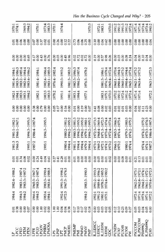
LP 0.01 1984:4 1982:4-1988:2 0.01 1981:3 1981:1-1982:1 0.00 1982:1 1981:4-1984:1 0.00 0.01 1970:1 LPCC 0.38 0.01 1966:3 1966:1-1967:1 0.00 1984:1 1983:3-1986:3 0.00 0.00 1974:1 LPED 0.00 1984:3 1983:1-1987:4 0.34 0.00 1983:3 1983:2-1985:4 0.00 0.06 LPEM 0.00 1984:2 1983:3-1987:2 0.08 0.00 1983:1 1982:4-1984:4 0.00 0.00 1969:3 LPEN 0.07 0.02 1995:1 1994:3-1995:3 0.00 1984:2 1983:4-1986:2 0.65 0.00 1984:2
LPFR 0.00 1966:4 1965:3-1967:1 0.00 1987:2 1986:4-1987:4 0.38 0.17 0.07 LPGD 0.00 1984:2 1983:2-1987:4 0.24 0.00 1982:1 1981:4-1984:1 0.00 0.00 1970:1 LPGOV 1.00 0.49 0.79 0.43 0.37 LPHRM 0.02 1983:4 1983:3-1990:4 0.04 1995:1 1994:3-1995:3 0.00 1983:3 1982:4-1986:4 0.00 0.02 1973:4 LPMOSA 0.00 1984:1 1983:4-1988:3 0.61 0.00 1983:3 1983:1-1985:3 0.76 0.01 1983:3
LPS 1.00 0.27 0.05 1978:2 1976:4-1982:4 0.00 0.00 1970:1 LPSP 1.00 0.41 0.17 0.03 0.26 LPT 0.04 1992:4 1991:3-1998:2 0.28 0.00 1991:1 1990:3-1993:2 0.00 0.00 1974:4 PMCP 0.04 1972:3 1967:3-1974:3 0.01 1980:4 1980:2-1981:2 0.16 0.45 0.12 PMDEL 0.38 0.00 1994:4 1994:2-1995:2 0.00 1981:4 1981:3-1983:2 0.96 0.22
PMEMP 0.17 0.01 1981:1 1980:3-1981:3 0.01 1983:1 1982:3-1986:3 0.02 0.73 PMI 0.10 0.00 1994:4 1994:2-1995:2 0.00 1984:4 1984:2-1987:4 0.72 0.06 PMNO 0.17 0.00 1994:4 1994:2-1995:2 0.19 0.02 0.06 PMNV 0.02 1984:2 1983:3-1990:3 0.00 1979:3 1979:1-1980:1 0.00 1977:1 1976:3-1978:2 0.72 0.25 PMP 0.18 0.00 1994:4 1994:2-1995:2 0.07 0.00 0.00 1970:3
R-LEHCC 0.00 1992:1 1991:2-1993:3 0.00 1973:1 1972:3-1973:3 0.41 0.19 0.10 LEHCC 0.03 1991:2 1989:4-1996:2 0.05 1969:2 1968:4-1969:4 0.08 0.00 0.00 1972:1 R-LEHM 0.03 1980:1 1978:2-1985:2 0.00 1972:1 1971:3-1972:3 0.00 1983:1 1981:3-1986:1 0.57 0.04 1983:1 LEHM 0.02 1975:1 1974:4-1980:2 0.01 1974:2 1973:4-1974:4 0.02 1975:1 1974:3-1978:4 0.98 0.62 GDC 0.05 0.02 1973:2 1972:4-1973:4 0.03 1970:3 1965:4-1972:4 0.06 0.00 1970:3
PUNEW 0.12 0.00 1966:1 1965:3-1966:3 0.01 1970:2 1960:1-1970:4 0.00 0.00 1991:2 PUXF 0.10 0.00 1975:2 1974:4-1975:4 0.02 1991:2 1990:4-1994:3 0.03 0.00 1991:2 PUXHS 0.23 0.08 0.01 1972:4 1960:1-1973:2 0.00 0.00 1991:3 PUXM 0.09 0.00 1980:1 1979:3-1980:3 0.03 1991:2 1990:4-1994:4 0.08 0.00 1991:2 PW 0.27 0.01 1974:4 1974:2-1975:2 0.00 1972:4 1965:1-1973:4 0.24 0.00 1972:4
PSCCOM 0.05 1972:4 1962:2-1973:1 0.21 0.04 1971:4 1962:1-1973:2 0.04 0.00 1971:4 R-PSCCOM 0.03 1971:4 1962:4-1972:1 0.13 0.02 1971:4 1963:4-1973:2 0.00 0.00 1971:4 PSM99Q 0.04 1973:4 1964:2-1974:1 0.01 1974:4 1974:2-1975:2 0.11 0.10 0.00 1973:4 R_PSM99Q 0.05 1971:4 1961:1-1972:1 0.01 1974:1 1973:3-1974:3 0.23 0.04 0.00 1973:4 PU83 0.00 1972:2 1970:4-1972:3 0.00 1987:2 1986:4-1987:4 0.00 1972:2 1963:1-1972:3 0.00 0.04 1990:2
m
a V, n
m
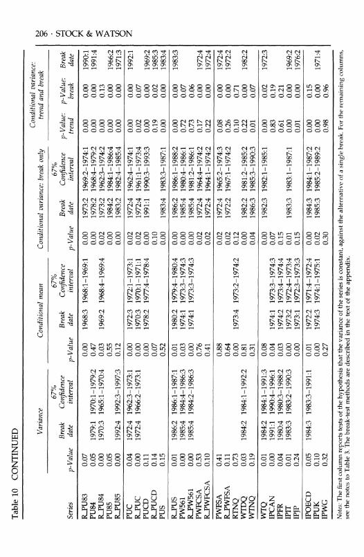
Table 10 CONTINUED
Conditional variance: Variance Conditional mean Conditional variance: break only trend and break
67% 67% 67% Break Confidence Break Confidence Break Confidence p-Value: p-Value: Break
Series p-Value date interval p-Value date interval p-Value date interval trend break date
R_PU83 0.07 0.00 1968:3 1968:1-1969:1 0.00 1973:2 1969:2-1974:1 0.00 0.00 1990:1 PU84 0.05 1979:1 1970:1-1979:2 0.47 0.00 1978:2 1968:4-1979:2 0.00 0.00 1991:4 R_PU84 0.00 1970:3 1965:1-1970:4 0.03 1969:2 1968:4-1969:4 0.02 1973:2 1962:3-1974:2 0.00 0.13 PU85 0.05 0.55 0.00 1984:2 1984:1-1986:4 0.00 0.00 1966:2 RJPU85 0.00 1992:4 1992:3-1997:3 0.12 0.00 1983:2 1982:4-1985:4 0.00 0.00 1971:3 PUC 0.04 1972:4 1962:3-1973:1 0.00 1972:3 1972:1-1973:1 0.02 1972:4 1962:4-1974:1 0.00 0.00 1992:1 R_PUC 0.00 1972:4 1966:2-1973:1 0.00 1970:3 1970:1-1971:1 0.02 1972:4 1961:1-1973:4 0.02 0.07 PUCD 0.11 0.00 1978:2 1977:4-1978:4 0.00 1991:1 1990:3-1993:3 0.00 0.00 1969:2 R-PUCD 0.14 0.07 0.10 0.19 0.02 1985:3 PUS 0.15 0.52 0.00 1983:4 1983:3-1987:1 0.00 0.00 1983:4 R-PUS 0.01 1986:2 1986:1-1987:1 0.01 1980:2 1979:4-1980:4 0.00 1986:2 1986:1-1988:2 0.00 0.00 1983:3 PW561 0.00 1985:4 1984:4-1986:3 0.03 1974:1 1973:3-1974:3 0.00 1985:4 1980:4-1986:1 0.72 0.07 R_PW561 0.00 1985:4 1984:2-1986:3 0.00 1974:1 1973:3-1974:3 0.00 1985:4 1981:2-1986:1 0.73 0.06 PWFCSA 0.53 0.76 0.02 1972:4 1964:4-1974:2 0.17 0.00 1972:4 R_PWFCSA 0.10 0.41 0.02 1972:4 1964:1-1974:2 0.22 0.00 1972:4 PWFSA 0.41 0.88 0.02 1972:4 1965:2-1974:3 0.08 0.00 1972:4 R_PWFSA 0.11 0.64 0.02 1972:2 1967:1-1974:2 0.26 0.00 1972:2 RTNQ 0.73 0.00 1973:4 1973:2-1974:2 0.12 0.10 0.71 WTDQ 0.03 1984:2 1984:1-1992:2 0.81 0.00 1982:2 1981:2-1985:2 0.22 0.00 1982:2 WTNQ 0.19 0.31 0.04 1986:3 1985:3-1990:3 0.01 0.07 WTQ 0.01 1984:2 1984:1-1991:3 0.08 0.00 1982:3 1982:1-1985:1 0.00 0.02 1972:3 IPCAN 0.00 1991:1 1990:4-1996:1 0.04 1974:1 1973:3-1974:3 0.07 0.83 0.19 IPFR 0.04 1980:4 1980:3-1988:2 0.03 1974:2 1973:4-1974:4 0.15 0.61 0.21 IPIT 0.01 1983:3 1983:2-1990:3 0.00 1973:2 1972:4-1973:4 0.01 1983:3 1983:1-1987:1 0.00 0.00 1969:2 IPJP 0.24 0.00 1973:1 1972:3-1973:3 0.15 0.01 0.00 1976:2
IPOECD 0.05 1984:3 1983:3-1991:1 0.01 1972:2 1971:4-1972:4 0.00 1984:3 1984:1-1987:2 0.00 0.15 IPUK 0.10 0.00 1974:3 1974:1-1975:1 0.02 1985:3 1985:2-1989:2 0.00 0.00 1971:4 IPWG 0.32 0.27 0.30 0.98 0.96
Notes: The first column reports tests of the hypothesis that the variance of the series is constant, against the alternative of a single break. For the remaining columns, see the notes to Table 3. The break-test methods are described in the text of the appendix.
O" (.
0
cZ C,)
z
Has the Business Cycle Changed and Why? ? 207
where Et, llt,..., Tlpt are i.i.d. N(0, 1) and independently distributed, and where it is distributed independently of the other shocks. To allow for large jumps in the instantaneous innovation variance t
2 (and thereby capture a possible break in the variance), we use a mixture-of-normals model for ,t; specifically, t i distributed N(0, r2) with probability q and N(0, r2) with probability 1 - q. The series yt is standardized before the
computations, and we set Cj = 7/T, a value consistent with previous estimates of parameter drift in autoregressions. For these calculations, we set t1 = 0.04, T2 = 0.2, q = 0.95, and p = 4.
The non-Gaussian smoother for the time-varying parameters is com-
puted using Markov-chain Monte Carlo (MCMC) methods. Let Y denote
yi, ? , T, let A denote {jt, j = 1,..., p, t = 1,..., T), and let S denote G1,. .., oTr. The MCMC algorithm iterates between the three conditional distributions of YIA, S, of AlY, S, and of S A, Y. The first two of these conditional distributions are normal, given the stated assumptions. The third distribution, however, is non-normal and-as suggested by Shep- hard (1994)-is computed by approximating the distribution of In e? (which is the distribution of the logarithm of a chi-squared random vari- able with one degree of freedom) by a mixture-of-normals distribution; the means and variances of the mixture (and the mixture weights) were chosen to match the first four moments of the log X2 distribution. Initial conditions were set using a flat prior, and a diffuse conjugate prior was used for the parameter values.
Given the smoothed parameter values, the estimated instantaneous au- tocovariances of yt are computed using O2T and ajtlT, the conditional means of ct and aoj given yl, . . ., Y. The smoothed instantaneous variances of
four-quarter growth rates were computed by temporal aggregation of the instantaneous autocovariance function.
A.2 VARIANCE-BREAK TESTS
To test for a break in the unconditional variance (the first column of Table 10), the absolute value of the demeaned series (e.g., the absolute value of demeaned four-quarter growth in GDP) was regressed against a constant and a binary variable 1 (t - z) for the break date. The QLR statistic is the squared heteroscedasticity- and autocorrelation-robust t-statistic on the break indicator, maximized over T in the central 70% of the sample.
The tests for a break in the conditional variance were computed as fol- lows. Let et(K) denote the errors in the autoregression in (1), where the AR coefficients break at date K, and let ?t(K) denote the OLS residuals estimated with a break in the AR coefficients at date K. Under the null hypothesis that there is no break in the variance, E I ?t(K) I is constant; under the alternative hypothesis that there is a break at date ', we have El Et(K) I =

208 ? STOCK & WATSON
(o + X l(t - z), where o1 is the first-period standard deviation and X is the difference between the standard deviations before and after the break. We therefore test for a break by computing the QLR statistic in the regres- sion of I?(K) I against a constant and the binary variable l(t - t), using homoscedastic standard errors (which are valid under the null), where K
is the least-squares estimator of the break date in the AR coefficients. Ta- ble 3 also reports results for a trend-augmented version of this regression, in which I?t(K)I was regressed against a constant, l(t 'r), and the time trend t, as well as the p-value for the test that the coefficient on t is zero in the regression in which T = T. Critical values for the QLR statistic [the squared t-statistic on l(t - z), maximized over z] in this trend-augmented regression were computed by Monte Carlo simulation. In all cases, the search over T was conducted in the central 70% of the sample.
Confidence intervals for the conditional-variance break date were com-
puted using the least-squares estimator from the regression of I?f(iK) against a constant and l(t >- ). If there is a break, the variance of the error term in this regression differs before and after the break, requiring a modification to Bai's (1997) limiting distribution for the least-squares break-date estimator. This modification entails scaling the distribution
differently on either side of the break, by the appropriate estimated vari- ance. The confidence interval for the break date is then obtained by in-
verting the test of the break date, based on this distribution. This results in asymmetric confidence intervals that express greater uncertainty about the break date in the low- than in the high-volatility period. The same method applies to the unconditional-variance break date, except the de-
pendent variable is the absolute value of the demeaned series and HAC standard errors are used as discussed in Bai (1997).
Results for all 168 series are summarized in Table 10.
Appendix B. Data
Table 11 lists the time series used in the empirical analysis. The series were either taken directly from the DRI-McGraw Hill Basic Economics database, in which case the original mnemonics are used, or produced by authors' calculations based on data from that database, in which case the authors' calculations and original DRI-McGraw Hill series mnemon- ics are summarized in the data description field. Following the series name is a transformation code and a short data description. The transfor- mations are (1) level of the series; (2) first difference; (3) second difference; (4) logarithm of the series; (5) first difference of the logarithm; (6) sec- ond difference of the logarithm. The following abbreviations appear in the data descriptions: sa = seasonally adjusted; nsa = not seasonally
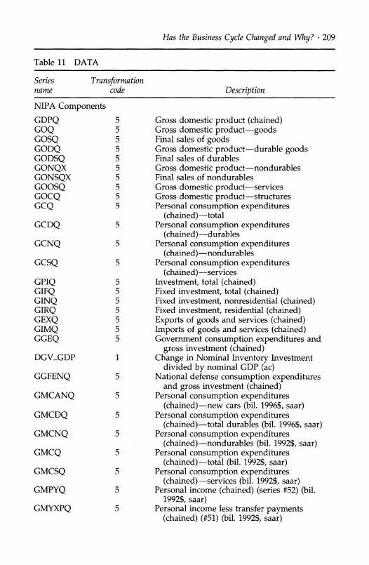
Has the Business Cycle Changed and Why? ? 209
Table 11 DATA
Series Transformation name code Description
NIPA Components
GDPQ GOQ GOSQ GODQ GODSQ GONQX GONSQX GOOSQ GOCQ GCQ
GCDQ
GCNQ
GCSQ
GPIQ GIFQ GINQ GIRQ GEXQ GIMQ GGEQ
DGV_GDP
GGFENQ
GMCANQ
GMCDQ
GMCNQ
GMCQ
GMCSQ
GMPYQ
GMYXPQ
5 Gross domestic product (chained) 5 Gross domestic product-goods 5 Final sales of goods 5 Gross domestic product-durable goods 5 Final sales of durables 5 Gross domestic product-nondurables 5 Final sales of nondurables 5 Gross domestic product-services 5 Gross domestic product-structures 5 Personal consumption expenditures
(chained)-total 5 Personal consumption expenditures
(chained)-durables 5 Personal consumption expenditures
(chained)-nondurables 5 Personal consumption expenditures
(chained)-services 5 Investment, total (chained) 5 Fixed investment, total (chained) 5 Fixed investment, nonresidential (chained) 5 Fixed investment, residential (chained) 5 Exports of goods and services (chained) 5 Imports of goods and services (chained) 5 Government consumption expenditures and
gross investment (chained) 1 Change in Nominal Inventory Investment
divided by nominal GDP (ac) 5 National defense consumption expenditures
and gross investment (chained) 5 Personal consumption expenditures
(chained)-new cars (bil. 1996$, saar) 5 Personal consumption expenditures
(chained)-total durables (bil. 1996$, saar) 5 Personal consumption expenditures
(chained)-nondurables (bil. 1992$, saar) 5 Personal consumption expenditures
(chained)-total (bil. 1992$, saar) 5 Personal consumption expenditures
(chained)-services (bil. 1992$, saar) 5 Personal income (chained) (series #52) (bil.
1992$, saar) 5 Personal income less transfer payments
(chained) (#51) (bil. 1992$, saar)
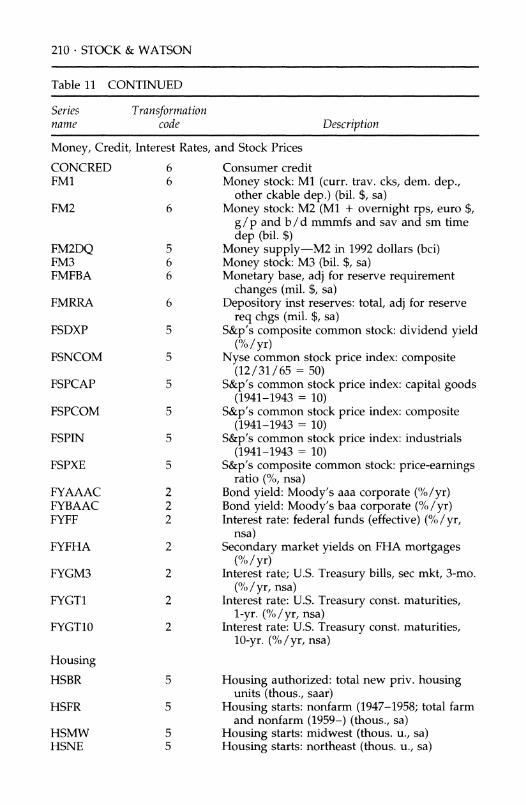
210 STOCK & WATSON
Table 11 CONTINUED
Series Transformation name code Description
Money, Credit, Interest Rates, and Stock Prices
6 Consumer credit 6 Money stock: M1 (curr. trav. cks, dem. dep.,
other ckable dep.) (bil. $, sa) 6 Money stock: M2 (M1 + overnight rps, euro $,
g/p and b/d mmmfs and sav and sm time dep (bil. $)
5 Money supply-M2 in 1992 dollars (bci) 6 Money stock: M3 (bil. $, sa) 6 Monetary base, adj for reserve requirement
changes (mil. $, sa) 6 Depository inst reserves: total, adj for reserve
req chgs (mil. $, sa) 5 S&p's composite common stock: dividend yield
(% / yr) 5 Nyse common stock price index: composite
(12/31/65 = 50) 5 S&p's common stock price index: capital goods
(1941-1943 = 10) 5 S&p's common stock price index: composite
(1941-1943 = 10) 5 S&p's common stock price index: industrials
(1941-1943 = 10) 5 S&p's composite common stock: price-earnings
ratio (%, nsa) 2 Bond yield: Moody's aaa corporate (%/yr) 2 Bond yield: Moody's baa corporate (%/yr) 2 Interest rate: federal funds (effective) (%/yr,
nsa) 2 Secondary market yields on FHA mortgages
(% / yr) 2 Interest rate; U.S. Treasury bills, sec mkt, 3-mo.
(% / yr, nsa) 2 Interest rate: U.S. Treasury const. maturities,
1-yr. (%/yr, nsa) 2 Interest rate: U.S. Treasury const. maturities,
10-yr. (%/yr, nsa)
5 Housing authorized: total new priv. housing units (thous., saar)
5 Housing starts: nonfarm (1947-1958; total farm and nonfarm (1959-) (thous., sa)
5 Housing starts: midwest (thous. u., sa) 5 Housing starts: northeast (thous. u., sa)
CONCRED FM1
FM2
FM2DQ FM3 FMFBA
FMRRA
FSDXP
FSNCOM
FSPCAP
FSPCOM
FSPIN
FSPXE
FYAAAC FYBAAC FYFF
FYFHA
FYGM3
FYGT1
FYGT10
Housing HSBR
HSFR
HSMW HSNE
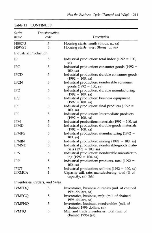
Has the Business Cycle Changed and Why? ? 211
Table 11 CONTINUED
Series Transformation name code
HSSOU 5 HSWST 5
Industrial Production
IP 5
IPC 5
IPCD 5
IPCN 5
IPD 5
IPE 5
IPF 5
IPI 5
IPM 5 IPMD 5
IPMFG 5
IPMIN 5 IPMND 5
IPN 5
IPP 5
IPUT 5 IPXMCA 1
Inventories, Orders, and Sales
IVMFDQ 5
IVMFGQ 5
IVMFNQ 5
IVMTQ 5
Description
Housing starts: south (thous. u., sa) Housing starts: west (thous. u., sa)
Industrial production: total index (1992 = 100, sa)
Industrial production: consumer goods (1992 = 100, sa)
Industrial production: durable consumer goods (1992 = 100, sa)
Industrial production: nondurable consumer
goods (1992 = 100, sa) Industrial production: durable manufacturing
(1992 = 100, sa) Industrial production: business equipment
(1992 = 100, sa) Industrial production: final products (1992 =
100, sa) Industrial production: Intermediate products
(1992 = 100, sa) Industrial production: materials (1992 = 100, sa) Industrial production: durable-goods materials
(1992 = 100, sa) Industrial production: manufacturing (1992 =
100, sa) Industrial production: mining (1992 = 100, sa) Industrial production: nondurable-goods mate-
rials (1992 = 100, sa) Industrial production: nondurable manufactur-
ing (1992 = 100, sa) Industrial production: products, total (1992 =
100, sa) Industrial production: utilities (1992 = 100, sa) Capacity util. rate: manufacturing, total (% of
capacity, sa) (frb)
Inventories, business durables (mil. of chained 1996 dollars, sa)
Inventories, business, mfg. (mil. of chained 1996 dollars, sa)
Inventories, business, nondurables (mil. of chained 1996 dollars, sa)
Mfg. and trade inventories: total (mil. of chained 1996) (sa)
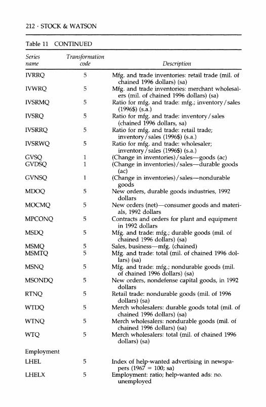
212 * STOCK & WATSON
Description
5 Mfg. and trade inventories: retail trade (mil. of chained 1996 dollars) (sa)
5 Mfg. and trade inventories: merchant wholesal- ers (mil. of chained 1996 dollars) (sa)
5 Ratio for mfg. and trade: mfg.; inventory/sales (1996$) (s.a.)
5 Ratio for mfg. and trade: inventory/sales (chained 1996 dollars, sa)
5 Ratio for mfg. and trade: retail trade; inventory/sales (1996$) (s.a.)
5 Ratio for mfg. and trade: wholesaler; inventory/sales (1996$) (s.a.)
1 (Change in inventories)/sales-goods (ac) 1 (Change in inventories)/sales-durable goods
(ac) 1 (Change in inventories)/ sales-nondurable
goods 5 New orders, durable goods industries, 1992
dollars 5 New orders (net)-consumer goods and materi-
als, 1992 dollars 5 Contracts and orders for plant and equipment
in 1992 dollars 5 Mfg. and trade: mfg.; durable goods (mil. of
chained 1996 dollars) (sa) 5 Sales, business-mfg. (chained) 5 Mfg. and trade: total (mil. of chained 1996 dol-
lars) (sa) 5 Mfg. and trade: mfg.; nondurable goods (mil.
of chained 1996 dollars) (sa) 5 New orders, nondefense capital goods, in 1992
dollars 5 Retail trade: nondurable goods (mil. of 1996
dollars) (sa) 5 Merch wholesalers: durable goods total (mil. of
chained 1996 dollars) (sa) 5 Merch wholesalers: nondurable goods (mil. of
chained 1996 dollars) (sa) 5 Merch wholesalers: total (mil. of chained 1996
dollars) (sa)
5 Index of help-wanted advertising in newspa- pers (1967 = 100; sa)
5 Employment: ratio; help-wanted ads: no. unemployed
Table 11 CONTINUED
Series Transformation name code
IVRRQ
IVWRQ
IVSRMQ
IVSRQ
IVSRRQ
IVSRWQ
GVSQ GVDSQ
GVNSQ
MDOQ
MOCMQ
MPCONQ
MSDQ
MSMQ MSMTQ
MSNQ
MSONDQ
RTNQ
WTDQ
WTNQ
WTQ
Employment LHEL
LHELX
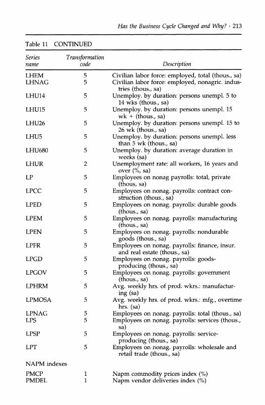
Has the Business Cycle Changed and Why? * 213
Table 11 CONTINUED
Series Transformation name code Description
5 Civilian labor force: employed, total (thous., sa) 5 Civilian labor force: employed, nonagric. indus-
tries (thous., sa) 5 Unemploy. by duration: persons unempl. 5 to
14 wks (thous., sa) 5 Unemploy. by duration: persons unempl. 15
wk + (thous., sa) 5 Unemploy. by duration: persons unempl. 15 to
26 wk (thous., sa) 5 Unemploy. by duration: persons unempl. less
than 5 wk (thous., sa) 5 Unemploy. by duration: average duration in
weeks (sa) 2 Unemployment rate: all workers, 16 years and
over (%, sa) 5 Employees on nonag payrolls: total, private
(thous, sa) 5 Employees on nonag. payrolls: contract con-
struction (thous., sa) 5 Employees on nonag. payrolls: durable goods
(thous., sa) 5 Employees on nonag. payrolls: manufacturing
(thous., sa) 5 Employees on nonag. payrolls: nondurable
goods (thous., sa) 5 Employees on nonag. payrolls: finance, insur.
and real estate (thous., sa) 5 Employees on nonag. payrolls: goods-
producing (thous., sa) 5 Employees on nonag. payrolls: government
(thous., sa) 5 Avg. weekly hrs. of prod. wkrs.: manufactur-
ing (sa) 5 Avg. weekly hrs. of prod. wkrs.: mfg., overtime
hrs. (sa) 5 Employees on nonag. payrolls: total (thous., sa) 5 Employees on nonag. payrolls: services (thous.,
sa) 5 Employees on nonag. payrolls: service-
producing (thous., sa) 5 Employees on nonag. payrolls: wholesale and
retail trade (thous., sa)
NAPM indexes
PMCP PMDEL
1 Napm commodity prices index (%) 1 Napm vendor deliveries index (%)
LHEM LHNAG
LHU14
LHU15
LHU26
LHU5
LHU680
LHUR
LP
LPCC
LPED
LPEM
LPEN
LPFR
LPGD
LPGOV
LPHRM
LPMOSA
LPNAG LPS
LPSP
LPT
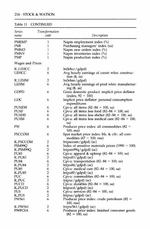
214 * STOCK & WATSON
Table 11 CONTINUED
Series Transformation name code Description
PMEMP PMI PMNO PMNV PMP
Wages and Prices
R-LEHCC LEHCC
R-LEHM LEHM
GDPD
GDC
PUNEW PUXF PUXHS PUXM
PW
PSCCOM
R-PSCCOM PSM99Q R_PSM99Q PU83 R_PU83 PU84 R-PU84 PU85 R-PU85 PUC R-PUC PUCD R_PUCD PUS R_PUS PW561
R-PW561 PWFCSA
1 1 1 1 1
Napm employment index (%) Purchasing managers' index (sa) Napm new orders index (%) Napm inventories index (%) Napm production index (%)
2 ln(lehcc/ gdpd) 6 Avg hourly earnings of constr wkrs: construc-
tion ($, sa) 2 ln(lehm/gdpd) 6 Avg hourly earnings of prod wkrs: manufactur-
ing ($, sa) 6 Gross domestic product: implicit price deflator
(index, 92 = 100) 6 Implicit price deflator: personal consumption
expenditures 6 Cpi-u: all items (82-84 = 100, sa) 6 Cpi-u: all items less food (82-84 = 100, sa) 6 Cpi-u: all items less shelter (82-84 = 100, sa) 6 Cpi-u: all items less medical care (82-84 = 100,
sa) 6 Producer price index: all commodities (82 =
100, nsa) 6 Spot market price index: bls. & crb.: all com-
modities (67 = 100, nsa) 2 ln(psccom/gdpd) (ac) 6 Index of sensitive materials prices (1990 = 100) 2 ln(psm99q/gdpd) (ac) 6 Cpi-u: apparel & upkeep (82-84 = 100, sa) 2 ln(pu83 / gdpd) (ac) 6 Cpi-u: transportation (82-84 = 100, sa) 2 ln(pu84/gdpd) (ac) 6 Cpi-u: medical care (82-84 = 100, sa) 2 ln(pu85 /gdpd) (ac) 6 Cpi-u: commodities (82-84 = 100, sa) 2 ln(puc / gdpd) (ac) 6 Cpi-u: durables (82-84 = 100, sa) 2 ln(pucd/gdpd) (ac) 6 Cpi-u: services (82-84 = 100, sa) 2 ln(pus / gdpd) (ac) 6 Producer price index: crude petroleum (82 =
100, nsa) 2 ln(pw561 /gdpd) (ac) 6 Producer price index: finished consumer goods
(82 = 100, sa)
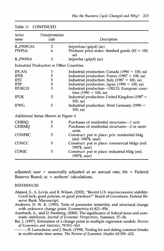
Has the Business Cycle Changed and Why? * 215
Table 11 CONTINUED
Series Transformation name code Description
R_PWFCSA 2 ln(pwfcsa/gdpd) (ac) PWFSA 6 Producer price index: finished goods (82 = 100,
sa) R_PWFSA 2 ln(pwfsa / gdpd) (ac)
Industrial Production in Other Countries
IPCAN 5 Industrial production: Canada (1990 = 100, sa) IPFR 5 Industrial production: France (1987 = 100, sa) IPIT 5 Industrial production: Italy (1987 = 100, sa) IPJP 5 Industrial production: Japan (1990 = 100, sa) IPOECD 5 Industrial production-OECD, European coun-
tries (1990 = 100, sa) IPUK 5 Industrial production: United Kingdom (1987 =
100, sa) IPWG 5 Industrial production: West Germany (1990 =
100, sa)
Additional Series Shown in Figure 4
GFIRSQ 5 Purchases of residential structures-1 unit GFIRMQ 5 Purchases of residential structures-2 or more
units CONFRC 5 Construct. put in place: priv residential bldg
(mil. 1987$, saar) CONCC 5 Construct. put in place: commercial bldgs (mil.
1987$, saar) CONIC 5 Construct. put in place: industrial bldg (mil.
1987$, saar)
adjusted; saar = seasonally adjusted at an annual rate; frb = Federal Reserve Board; ac = authors' calculations.
REFERENCES
Ahmed, S., A. Levin, and B. Wilson. (2002). "Recent U.S. macroeconomic stability: Good luck, good policies, or good practices?" Board of Governors, Federal Re- serve Bank. Manuscript.
Andrews, D. W. K. (1993). Tests of parameter instability and structural change with unknown change point. Econometrica 61:821-856.
Auerbach, A., and D. Feenberg. (2000). The significance of federal taxes and auto- matic stabilizers. Journal of Economic Perspectives, Summer, 37-56.
Bai, J. (1997). Estimation of a change point in multiple regression models. Review of Economics and Statistics 79:551-563.
,R. Lumsdaine, and J. Stock. (1998). Testing for and dating common breaks in multivariate time series. The Review of Economic Studies 65:395-432.
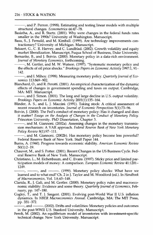
216 STOCK & WATSON
,and P. Perron. (1998). Estimating and testing linear models with multiple structural changes. Econometrica 66:47-78.
Basistha, A., and R. Startz. (2001). Why were changes in the federal funds rates smaller in the 1990s? University of Washington. Manuscript.
Basu, S., J. Fernald, and M. Kimball. (1999). Are technology improvements con- tractionary? University of Michigan. Manuscript.
Bekaert, G., C. R. Harvey, and C. Lundblad. (2002). Growth volatility and equity market liberalization. Manuscript, Fuqua School of Business, Duke University.
Beranke, B., and J. Boivin. (2000). Monetary policy in a data-rich environment. Journal of Monetary Economics, forthcoming.
, M. Gertler, and M. W. Watson. (1997). "Systematic monetary policy and the effects of oil price shocks." Brookings Papers on Economic Activity 1997:1, 91- 142.
and I. Mihoy. (1998). Measuring monetary policy. Quarterly Journal of Eco- nomics 113:869-902.
Blanchard, 0., and R. Perotti. (2001). An empirical characterization of the dynamic effects of changes in government spending and taxes on output. Cambridge, MA: MIT. Manuscript.
, and J. Simon. (2001). The long and large decline in U.S. output volatility. Brookings Papers on Economic Activity 2001(1):135-164.
Blinder, A. S., and L. J. Maccini. (1991). Taking stock: A critical assessment of recent research on inventories. Journal of Economic Perspectives 5(1):73-96.
Boivin, J. (2000). The Fed's conduct of monetary policy: Has it changed and does it matter? Essays on the Analysis of Changes in the Conduct of Monetary Policy. Princeton University. PhD Dissertation, Chapter 3.
, and M. Giannoni. (2002a). Assessing changes in the monetary transmis- sion mechanism: A VAR approach. Federal Reserve Bank of New York Monetary Policy Review 8(1):97-111.
, and M. Giannoni. (2002b). Has monetary policy become less powerful? Federal Reserve Bank of New York. Staff Paper 144.
Burns, A. (1960). Progress towards economic stability. American Economic Review 50(1):2-19.
Chauvet, M., and S. Potter. (2001). Recent Changes in the US Business Cycle. Fed- eral Reserve Bank of New York. Manuscript.
Christiano, L., M. Eichenbaum, and C. Evans. (1997). Sticky price and limited par- ticipation models of money: A comparison. European Economic Review 41:1201- 1249.
, , and . (1999). Monetary policy shocks: What have we learned and to what end? Ch. 2 in J. Taylor and M. Woodford (ed.). In Handbook of Macroeconomics, Vol. 1A:65-148.
Clarida, R., J. Gali, and M. Gertler. (2000). Monetary policy rules and macroeco- nomic stability: Evidence and some theory. Quarterly Journal of Economics, Feb- ruary, pp. 147-180.
Cogley, T., and T. J. Sargent. (2001). Evolving post-World War II U.S. inflation dynamics. In NBER Macroeconomics Annual. Cambridge, MA: The MIT Press, pp. 331-372.
,and . (2002). Drifts and volatilities: Monetary policies and outcomes in the post-WWII U.S. Stanford University. Manuscript.
Feroli, M. (2002). An equilibrium model of inventories with investment-specific technical change. New York University. Manuscript.
Has the Business Cycle Changed and Why? ? 217
Gali, J. (1999). Technology, employment and the business cycle: Do technology shocks explain aggregate productivity. American Economic Review 89:249- 271.
,and M. Gertler. (1999). Inflation dynamics: A structural econometric analy- sis. Journal of Monetary Economics 44:195-222.
, J. D. Lopez-Salido, and J. Valles. (2002). Technology shock and monetary policy: Assessing the Fed's performance. Cambridge, MA: National Bureau of Economic Research. NBER Working Paper 8768.
Gilchrist, S., and A. Kashyap. (1990). Assessing the smoothness of recent GNP growth. Internal memorandum, Board of Governors of the Federal Reserve System.
Golub, J. E. (2000). Post-1984 inventories revitalize the production-smoothing model. University of Missouri-Kansas City. Manuscript.
Goodfriend, M., and R. King. (1997). The New Neoclassical Synthesis and the Role of Monetary Policy. In NBER Macroeconomics Annual. Cambridge, MA: The MIT Press.
Hamilton, J. D. (1996). This is what happened to the oil price-macroeconomy rela- tionship. Journal of Monetary Economics 38(2):215-220.
Hansen, B. (2001). Testing for structural change in conditional models. Journal of Econometrics 97:93-115.
Herrera, A. M., and E. Pesavento. (2002). The decline in US output volatility: Structural changes in inventories or sales? Michigan State University. Manu- script.
Kahn, J., M. M. McConnell, and G. Perez-Quiros. (2001). The reduced volatility of the U.S. economy: Policy or progress? Federal Reserve Bank of New York. Manuscript.
, , and . (2002). On the causes of the increased stability of the U.S. economy. Federal Reserve Bank of New York Economic Policy Review 8(1):183- 202.
Kim, C.-J., and C. R. Nelson. (1999). Has the U.S. economy become more stable? A Bayesian approach based on a Markov-switching model of the business cycle. The Review of Economics and Statistics 81:608-616.
, , and J. Piger. (2001). The less volatile U.S. economy: A Bayesian investigation of breadth, and potential explanations. Board of Governors of the Federal Reserve System. International Finance Discussion Paper 707.
McCarthy, J., and R. W. Peach. (2002). Monetary policy transmission to residential investment. Federal Reserve Bank of New York Economic Policy Review 8(1):139- 158.
McConnell, M. M., and G. Perez-Quiros. (2000). Output fluctuations in the United States: What has changed since the early 1980's? American Economic Review 90(5): 1464-1476.
Moore, G. H., and V. Zarnowitz. (1986). The development and role of the NBER's business cycle chronologies. In The American Business Cycle: Continuity and Change, R. J. Gordon (ed.). Chicago: University of Chicago Press.
Pagan, A. (2000). Some thoughts on trend and cycle. Australian National Univer- sity. Manuscript.
Pivetta, F., and R. Reis. (2001). The persistence of inflation in the U.S. Department of Economics, Harvard University. Manuscript.
Primiceri, G. (2000). Time varying structural vector autoregressions and monetary policy. Princeton University. Manuscript.
218 * STOCK & WATSON
,and M. Woodford. (1999). Interest rate rules in an estimated sticky price model. In Monetary Policy Rules, J. Taylor (ed.). University of Chicago Press.
Quandt, R. E. (1960). Tests of the hypothesis that a linear regression obeys two separate regimes. Journal of the American Statistical Association 55:324-330.
Ramey, V. A., and D. J. Vine. (2001). Tracking the source of the decline in GDP volatility: An analysis of the automobile industry. University of California, San Diego. Manuscript.
,and K. D. West. (1999). Inventories. In Handbook of Macroeconomics, J. Tay- lor and M. Woodford (eds.). Vol. 1B, pp. 863-923.
Rotemberg, J., and M. Woodford. (1997). An optimization-based econometric framework for the evaluation of monetary policy. In NBER Macroeconomics An- nual. Cambridge, MA: The MIT Press. 297-345.
Rudebusch, G. D. (1998). Do measures of monetary policy in a VAR make sense? International Economic Review 39:907-931.
. (2002). Assessing nominal income rules for monetary policy with model and data uncertainty. The Economic Journal 112:402-432.
,and L. Svensson. (1999). Rules for inflation targeting. In Monetary Policy Rules, J. Taylor (ed.). University of Chicago Press.
Sensier, M., and D. van Dijk. (2001). Short-term volatility versus long-term growth: Evidence in US macroeconomic time series. University of Manchester. Manu- script.
Shephard, N. (1994). Partial non-Gaussian state space. Biometrika 81(1):115-131. Simon, J. (2000). The long boom. Essays in Empirical Macroeconomics. Cambridge,
MA: MIT. PhD Dissertation, Chapter 1. (2001). The decline in Australian output volatility. Reserve Bank of Austra-
lia. Manuscript. Sims, C. (2001). Stability and instability in US monetary policy behavior. Princeton
University. Manuscript. ,and T. Zha. (2002). Macroeconomic switching. Princeton University.
Manuscript. Staiger, D., M. W. Watson, and J. H. Stock. (2001). Prices, wages and the U.S.
NAIRU in the 1990s, Ch. 1 in The Roaring Nineties, A. Krueger and R. Solow (eds.), Russell Sage Foundation/The Century Fund: New York, 3-60.
Stock, J. H., and M. W. Watson. (1996). Evidence on structural instability in macroeco- nomic time series relations. Journal of Business and Economic Statistics 14:11-29.
,and . (1998). Asymptotically median unbiased estimation of coeffi- cient variance in a time varying parameter model. Journal of the American Statisti- cal Association 93:349-358.
,and . (1999). Forecasting inflation. Journal of Monetary Economics 44: 293-335.
,and . (2001). Macroeconomic forecasting using diffusion indexes. Journal of Business and Economic Statistics, forthcoming.
(1999b). An historical analysis of monetary policy rules. In Taylor (1999a). . (2000). Remarks for the panel discussion on recent changes in trend and
cycle. Stanford University. Manuscript. Warnock, M. V. C., and F. E. Warock. (2001). The declining volatility of U.S.
employment: Was Arthur Burns right? Board of Governors of the Federal Re- serve System. Manuscript.
Watson M. (1999). Explaining the increased variability in the long-term interest rate. Economic Quarterly (Federal Reserve Bank of Richmond) 85(Fall).
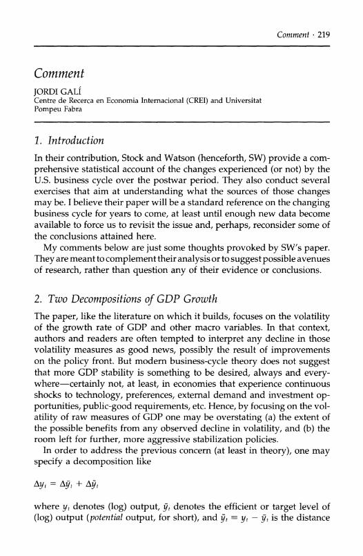
Comment * 219
Comment JORDI GALI Centre de Recerca en Economia Intemacional (CREI) and Universitat Pompeu Fabra
1. Introduction
In their contribution, Stock and Watson (henceforth, SW) provide a com-
prehensive statistical account of the changes experienced (or not) by the U.S. business cycle over the postwar period. They also conduct several exercises that aim at understanding what the sources of those changes may be. I believe their paper will be a standard reference on the changing business cycle for years to come, at least until enough new data become available to force us to revisit the issue and, perhaps, reconsider some of the conclusions attained here.
My comments below are just some thoughts provoked by SW's paper. They are meant to complement their analysis or to suggest possible avenues of research, rather than question any of their evidence or conclusions.
2. Two Decompositions of GDP Growth
The paper, like the literature on which it builds, focuses on the volatility of the growth rate of GDP and other macro variables. In that context, authors and readers are often tempted to interpret any decline in those
volatility measures as good news, possibly the result of improvements on the policy front. But modern business-cycle theory does not suggest that more GDP stability is something to be desired, always and every- where-certainly not, at least, in economies that experience continuous shocks to technology, preferences, external demand and investment op- portunities, public-good requirements, etc. Hence, by focusing on the vol-
atility of raw measures of GDP one may be overstating (a) the extent of the possible benefits from any observed decline in volatility, and (b) the room left for further, more aggressive stabilization policies.
In order to address the previous concern (at least in theory), one may specify a decomposition like
Ayt = Ayt + Ayt
where yt denotes (log) output, yt denotes the efficient or target level of (log) output (potential output, for short), and y t yt - yt is the distance
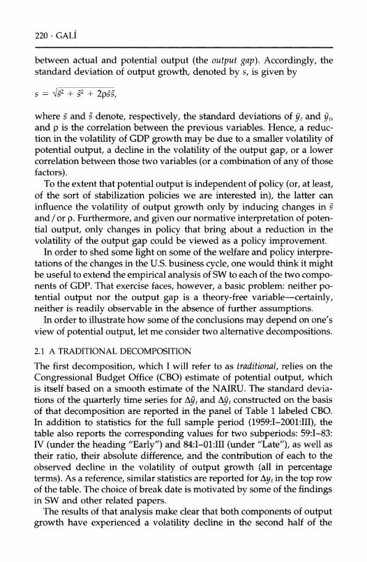
220 GALI
between actual and potential output (the output gap). Accordingly, the standard deviation of output growth, denoted by s, is given by
s = -l2 + s2 + 2pss,
where s and s denote, respectively, the standard deviations of yt and yt, and p is the correlation between the previous variables. Hence, a reduc- tion in the volatility of GDP growth may be due to a smaller volatility of
potential output, a decline in the volatility of the output gap, or a lower correlation between those two variables (or a combination of any of those factors).
To the extent that potential output is independent of policy (or, at least, of the sort of stabilization policies we are interested in), the latter can influence the volatility of output growth only by inducing changes in s and/or p. Furthermore, and given our normative interpretation of poten- tial output, only changes in policy that bring about a reduction in the
volatility of the output gap could be viewed as a policy improvement. In order to shed some light on some of the welfare and policy interpre-
tations of the changes in the U.S. business cycle, one would think it might be useful to extend the empirical analysis of SW to each of the two compo- nents of GDP. That exercise faces, however, a basic problem: neither po- tential output nor the output gap is a theory-free variable-certainly, neither is readily observable in the absence of further assumptions.
In order to illustrate how some of the conclusions may depend on one's view of potential output, let me consider two alternative decompositions.
2.1 A TRADITIONAL DECOMPOSITION
The first decomposition, which I will refer to as traditional, relies on the
Congressional Budget Office (CBO) estimate of potential output, which is itself based on a smooth estimate of the NAIRU. The standard devia- tions of the quarterly time series for Ayt and Ayt constructed on the basis of that decomposition are reported in the panel of Table 1 labeled CBO. In addition to statistics for the full sample period (1959:I-2001:III), the table also reports the corresponding values for two subperiods: 59:1-83: IV (under the heading "Early") and 84:I-01:III (under "Late"), as well as their ratio, their absolute difference, and the contribution of each to the observed decline in the volatility of output growth (all in percentage terms). As a reference, similar statistics are reported for Ayt in the top row of the table. The choice of break date is motivated by some of the findings in SW and other related papers.
The results of that analysis make clear that both components of output growth have experienced a volatility decline in the second half of the
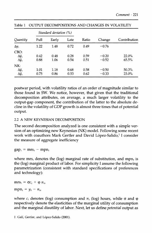
Comment * 221
Table 1 OUTPUT DECOMPOSITIONS AND CHANGES IN VOLATILITY
Standard deviation (%)
Quantity Full Early Late Ratio Change Contribution
Ayt 1.22 1.48 0.72 0.49 -0.76
CBO: Ayt 0.42 0.48 0.28 0.59 -0.20 22.0% Ayt 0.88 1.06 0.54 0.51 -0.52 65.5%
NK: Ayt 1.01 1.18 0.68 0.58 -0.50 50.3% Agt 0.75 0.86 0.53 0.62 -0.33 23.0%
postwar period, with volatility ratios of an order of magnitude similar to those found in SW. We notice, however, that given that the traditional
decomposition attributes, on average, a much larger volatility to the
output-gap component, the contribution of the latter to the absolute de- cline in the volatility of GDP growth is almost three times that of potential output.
2.2 A NEW KEYNESIAN DECOMPOSITION
The second decomposition analyzed is one consistent with a simple ver- sion of an optimizing new Keynesian (NK) model. Following some recent work with coauthors Mark Gertler and David Lopez-Salido,1 I consider the measure of aggregate inefficiency
gapt = mrst - mpnt
where mrst denotes the (log) marginal rate of substitution, and mpnt is the (log) marginal product of labor. For simplicity I assume the following parametrization (consistent with standard specifications of preferences and technology):
mrst = oct + P nt,
mpnt = yt - nt,
where ct denotes (log) consumption and nt (log) hours, while a and (p respectively denote the elasticities of the marginal utility of consumption and the marginal disutility of labor. Next, let us define potential output as
1. Gali, Gertler, and L6pez-Salido (2001).
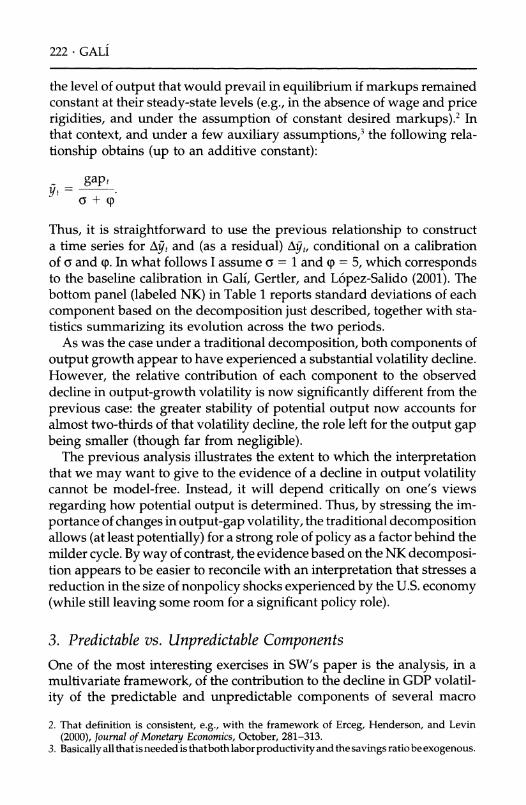
222 * GALI
the level of output that would prevail in equilibrium if markups remained constant at their steady-state levels (e.g., in the absence of wage and price rigidities, and under the assumption of constant desired markups).2 In that context, and under a few auxiliary assumptions,3 the following rela- tionship obtains (up to an additive constant):
gapt
aY + (
Thus, it is straightforward to use the previous relationship to construct a time series for Ayt and (as a residual) Agt, conditional on a calibration of a and (p. In what follows I assume a = 1 and (p = 5, which corresponds to the baseline calibration in Gali, Gertler, and Lopez-Salido (2001). The bottom panel (labeled NK) in Table 1 reports standard deviations of each component based on the decomposition just described, together with sta- tistics summarizing its evolution across the two periods.
As was the case under a traditional decomposition, both components of output growth appear to have experienced a substantial volatility decline. However, the relative contribution of each component to the observed decline in output-growth volatility is now significantly different from the previous case: the greater stability of potential output now accounts for almost two-thirds of that volatility decline, the role left for the output gap being smaller (though far from negligible).
The previous analysis illustrates the extent to which the interpretation that we may want to give to the evidence of a decline in output volatility cannot be model-free. Instead, it will depend critically on one's views regarding how potential output is determined. Thus, by stressing the im- portance of changes in output-gap volatility, the traditional decomposition allows (at least potentially) for a strong role of policy as a factor behind the milder cycle. By way of contrast, the evidence based on the NK decomposi- tion appears to be easier to reconcile with an interpretation that stresses a reduction in the size of nonpolicy shocks experienced by the U.S. economy (while still leaving some room for a significant policy role).
3. Predictable vs. Unpredictable Components One of the most interesting exercises in SW's paper is the analysis, in a multivariate framework, of the contribution to the decline in GDP volatil- ity of the predictable and unpredictable components of several macro
2. That definition is consistent, e.g., with the framework of Erceg, Henderson, and Levin (2000), Journal of Monetary Economics, October, 281-313.
3. Basically all that is needed is thatboth labor productivity and the savings ratio be exogenous.

Comment * 223
time series. SW conclude that changes in the unpredictable component (reflected in the variance-covariance matrix E of reduced-form VAR innovations) seem to have played a dominant role. In a structural VAR framework, however, changes in E must be caused by changes in the variance-covariance matrix of structural shocks, and/or changes in the matrix of contemporaneous relationships among the different variables. That observation raises an interesting question, which is briefly addressed in Blanchard and Simon (2001), but not in SW's paper: if we agree that mone-
tary policy affects aggregate demand and output only with a lag (an as-
sumption often incorporated in structural VARs), is it possible to reconcile the dominant role of the unpredictable component detected by SW with the
policy-improvement hypothesis (e.g., a more aggressive Taylor rule)? In my opinion that question can only be addressed using an explicit
structural model with an embedded policy rule of the sort used by SW in the last section of their paper. The SW model, however, may not be suitable to address the question posed above, since it does not incorporate any policy transmission lags. Perhaps a more realistic model incorporat- ing those lags [like those of Rotemberg and Woodford (1999), or Chris- tiano, Eichenbaum, and Evans (2001)] could be used in future research to reexamine the role of policy, in light of SW's evidence pointing to a domi- nant role of the unpredictable component as an immediate factor behind the changing volatility of U.S. GDP growth.
4. The Cross-Country Dimension SW's paper, as well as much of the related literature, studies the phenom- enon of changes in the business cycle from a time-series perspective. But measures of macroeconomic volatility appear to vary across countries no less than they vary over time. Can we learn anything from the cross-
country evidence regarding the sources of the observed changes (over time) in the U.S. business cycle? Here I just want to point to some evidence reported by Acemoglu and Zilibotti (1997), and whose possible connec- tion with the issue at hand is, to say the least, intriguing. They provide rather strong evidence of a negative relationship across countries between their level of development (measured by per capita GDP) and their cycli- cal volatility (measured by the standard deviation of GDP growth).4 Fatas
4. Acemoglu and Zilibotti develop a model that explains their evidence as the result of the insufficient diversification of productive activities resulting from project indivisibilities, which is only overcome as an economy develops (possibly thanks to a sequence of favor- able shocks). Kraay and Ventura (2001) provide an alternative explanation based on the patterns of specialization during the process of development of an economy. While both stories may help explain the cross-sectional evidence, neither mechanism seems a plausi- ble candidate to explain the taming of the U.S. business cycle over the postwar period.
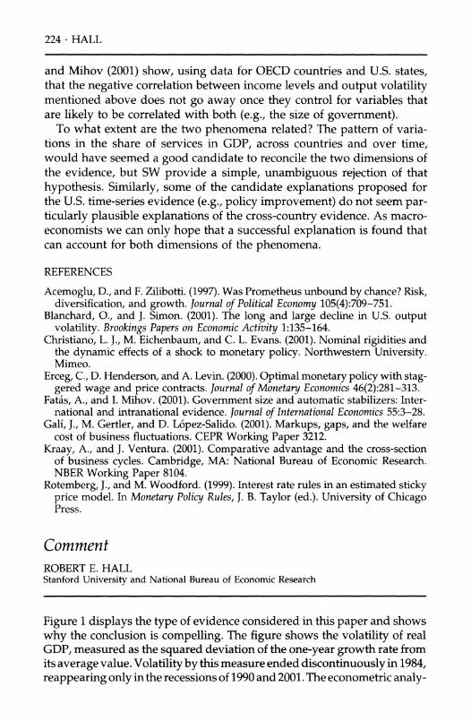
224 HALL
and Mihov (2001) show, using data for OECD countries and U.S. states, that the negative correlation between income levels and output volatility mentioned above does not go away once they control for variables that are likely to be correlated with both (e.g., the size of government).
To what extent are the two phenomena related? The pattern of varia- tions in the share of services in GDP, across countries and over time, would have seemed a good candidate to reconcile the two dimensions of the evidence, but SW provide a simple, unambiguous rejection of that hypothesis. Similarly, some of the candidate explanations proposed for the U.S. time-series evidence (e.g., policy improvement) do not seem par- ticularly plausible explanations of the cross-country evidence. As macro- economists we can only hope that a successful explanation is found that can account for both dimensions of the phenomena.
REFERENCES
Acemoglu, D., and F. Zilibotti. (1997). Was Prometheus unbound by chance? Risk, diversification, and growth. Journal of Political Economy 105(4):709-751.
Blanchard, O., and J. Simon. (2001). The long and large decline in U.S. output volatility. Brookings Papers on Economic Activity 1:135-164.
Christiano, L. J., M. Eichenbaum, and C. L. Evans. (2001). Nominal rigidities and the dynamic effects of a shock to monetary policy. Northwestern University. Mimeo.
Erceg, C., D. Henderson, and A. Levin. (2000). Optimal monetary policy with stag- gered wage and price contracts. Journal of Monetary Economics 46(2):281-313.
Fatas, A., and I. Mihov. (2001). Government size and automatic stabilizers: Inter- national and intranational evidence. Journal of International Economics 55:3-28.
Gali, J., M. Gertler, and D. L6pez-Salido. (2001). Markups, gaps, and the welfare cost of business fluctuations. CEPR Working Paper 3212.
Kraay, A., and J. Ventura. (2001). Comparative advantage and the cross-section of business cycles. Cambridge, MA: National Bureau of Economic Research. NBER Working Paper 8104.
Rotemberg, J., and M. Woodford. (1999). Interest rate rules in an estimated sticky price model. In Monetary Policy Rules, J. B. Taylor (ed.). University of Chicago Press.
Comment ROBERT E. HALL Stanford University and National Bureau of Economic Research
Figure 1 displays the type of evidence considered in this paper and shows why the conclusion is compelling. The figure shows the volatility of real GDP, measured as the squared deviation of the one-year growth rate from its average value. Volatility by this measure ended discontinuously in 1984, reappearing only in the recessions of 1990 and 2001. The econometric analy-
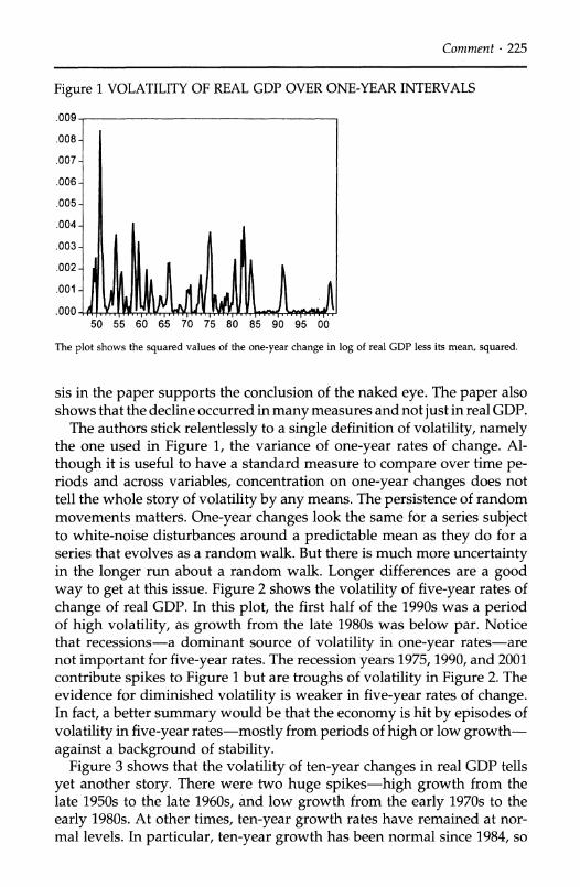
Comment 225
Figure 1 VOLATILITY OF REAL GDP OVER ONE-YEAR INTERVALS
.009
.008 -
.007 -
.006 -
.005 -
.004 -
.003-
.002 -
.001
.000 , 50 55 60 65 70 75 80 85 90 95 00
The plot shows the squared values of the one-year change in log of real GDP less its mean, squared.
sis in the paper supports the conclusion of the naked eye. The paper also shows that the decline occurred in many measures and not just in real GDP.
The authors stick relentlessly to a single definition of volatility, namely the one used in Figure 1, the variance of one-year rates of change. Al-
though it is useful to have a standard measure to compare over time pe- riods and across variables, concentration on one-year changes does not tell the whole story of volatility by any means. The persistence of random movements matters. One-year changes look the same for a series subject to white-noise disturbances around a predictable mean as they do for a series that evolves as a random walk. But there is much more uncertainty in the longer run about a random walk. Longer differences are a good way to get at this issue. Figure 2 shows the volatility of five-year rates of
change of real GDP. In this plot, the first half of the 1990s was a period of high volatility, as growth from the late 1980s was below par. Notice that recessions-a dominant source of volatility in one-year rates-are not important for five-year rates. The recession years 1975, 1990, and 2001 contribute spikes to Figure 1 but are troughs of volatility in Figure 2. The evidence for diminished volatility is weaker in five-year rates of change. In fact, a better summary would be that the economy is hit by episodes of
volatility in five-year rates-mostly from periods of high or low growth- against a background of stability.
Figure 3 shows that the volatility of ten-year changes in real GDP tells
yet another story. There were two huge spikes-high growth from the late 1950s to the late 1960s, and low growth from the early 1970s to the
early 1980s. At other times, ten-year growth rates have remained at nor- mal levels. In particular, ten-year growth has been normal since 1984, so
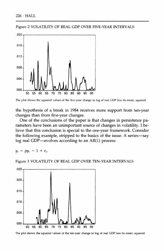
226 * HALL
Figure 2 VOLATILITY OF REAL GDP OVER FIVE-YEAR INTERVALS
.020
.016-
.012-
.008 -
.004 -
.000 ...... .. 50 55 60 65 70 75 80 85 90 95 00
The plot shows the squared values of the five-year change in log of real GDP less its mean, squared.
the hypothesis of a break in 1984 receives more support from ten-year changes than from five-year changes.
One of the conclusions of the paper is that changes in persistence pa- rameters have been an unimportant source of changes in volatility. I be- lieve that this conclusion is special to the one-year framework. Consider the following example, stripped to the basics of the issue. A series-say log real GDP-evolves according to an AR(1) process:
yt = PYt - 1 + Et.
Figure 3 VOLATILITY OF REAL GDP OVER TEN-YEAR INTERVALS
The plot shows the squared values of the ten-year change in log of real GDP less its mean, squared.
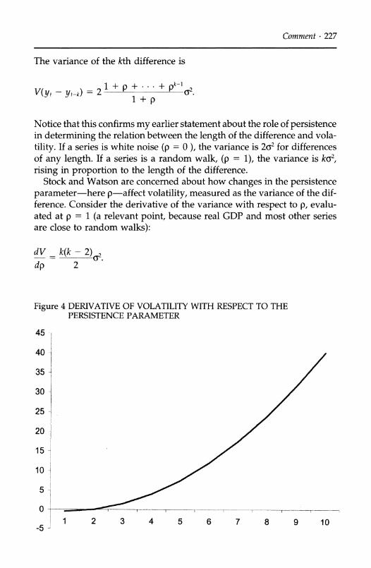
Comment . 227
The variance of the kth difference is
V(yt - yt-k) =2 l + +
Notice that this confirms my earlier statement about the role of persistence in determining the relation between the length of the difference and vola-
tility. If a series is white noise (p = 0 ), the variance is 2o2 for differences of any length. If a series is a random walk, (p = 1), the variance is ko2, rising in proportion to the length of the difference.
Stock and Watson are concerned about how changes in the persistence parameter-here p-affect volatility, measured as the variance of the dif- ference. Consider the derivative of the variance with respect to p, evalu- ated at p = 1 (a relevant point, because real GDP and most other series are close to random walks):
dV _ k(k - 2) 2
dp 2
Figure 4 DERIVATIVE OF VOLATILITY WITH RESPECT TO THE PERSISTENCE PARAMETER
45
40
35
30
25
20 i
15
10
5
O0 6 7 8 9 10
-5 1 2 3 4 5
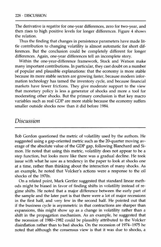
228 DISCUSSION
The derivative is negative for one-year differences, zero for two-year, and then rises to high positive levels for longer differences. Figure 4 shows the relation.
Thus the finding that changes in persistence parameters have made lit- tle contribution to changing volatility is almost automatic for short dif- ferences. But the conclusion could be completely different for longer differences. Again, one-year differences tell an incomplete story.
Within the one-year-difference framework, Stock and Watson make
many important contributions. In particular, they cast doubt on a number of popular and plausible explanations: that the economy is more stable because its more stable sectors are growing faster, because modem infor- mation technology has tamed the inventory cycle, and because financial markets have fewer frictions. They give moderate support to the view that monetary policy is less a generator of shocks and more a tool for
moderating other shocks. But the primary conclusion is that key macro variables such as real GDP are more stable because the economy suffers smaller outside shocks now than it did before 1984.
Discussion
Bob Gordon questioned the metric of volatility used by the authors. He
suggested using a gap-oriented metric such as the 20-quarter moving av-
erage of the absolute value of the GDP gap, following Blanchard and Si- mon. He noted that using this metric, volatility does not appear to be a
step function, but looks more like there was a gradual decline. He took issue with what he saw as a tendency in the paper to look at shocks one at a time, rather than thinking about the interaction of many shocks. As an example, he noted that Volcker's actions were a response to the oil shocks of the 1970s.
On a related point, Mark Gertler suggested that standard linear meth- ods might be biased in favor of finding shifts in volatility instead of re-
gime shifts. He noted that a major difference between the early part of the sample and the later part is that there were a lot of major recessions in the first half, and very few in the second half. He pointed out that if the business cycle is asymmetric in that contractions are sharper than
expansions, this might show up as a change in volatility rather than a shift in the propagation mechanism. As an example, he suggested that the recession of 1980-1982 could be plausibly attributed to the Volcker disinflation rather than to bad shocks. On the recession of 1974-1975 he noted that although the consensus view is that it was due to shocks, a
Discussion - 229
recent paper by Robert Barsky has argued otherwise. He was interested to see whether as a general rule the big recessions can be explained by shocks, and if so, what are the shocks. He also commented that any expla- nation of the reduction in output volatility must be consistent with the reduction in the volatility of inflation.
Jonathan Parker suggested that it might be interesting to see what sur-
vey forecast data have to say about reduced volatility. He pointed out that if economic forecasts lag, it might give a sense that the reduction in
volatility described in the paper was a surprise. In this case, it could be that a VAR would do a better job of fitting the data than actual expecta- tions over the period of the decline in volatility.
Justin Wolfers suggested a link between Gali and Hall's evidence on the reduction in the volatility of potential output and the output gap, and the debate about the Phillips curve in the session on Nancy Stokey's pa- per. He said that in order for the Phillips curve to describe the inflation
path of the 1990s, it is necessary to have enormous volatility in the natural rate of unemployment which cannot be squared with the observed reduc- tion in volatility. He also remarked that since the sample size used to
generate sectoral employment data triples over the period in question, it
might be safer to base decisions on sectoral differences on output shares rather than employment shares.
Fabrizio Perri remarked that it might be particularly useful to look at international data when trying to attribute the reduction in volatility to
changes in shocks or policy. He noted that there has also been a big de- cline in volatility in Europe. On this issue, Ken Rogoff mentioned that economists working at the IMF have produced evidence of a decline in the volatility of output and employment across the OECD. However, he noted that the volatility of stock prices has clearly not fallen. He specu- lated that this could imply that improvements in measurement over time are driving some of the observed reduction in volatility of GDP and
employment. Jean Boivin remarked that the IS curve in the structural model used
to evaluate the contribution of policy changes is very reduced-form. He worried that expectations of monetary policy are not sufficiently con- trolled for, leaving open the possibility that changes in monetary policy could contaminate the estimates of changes in volatility.
In summing up, Mark Watson welcomed the comments of Bob Hall and Bob Gordon on the question of regime break vs. slow decline in volatility. Ideally, he said, the authors would have liked to estimate linear models such as VARs, allowing for stochastic volatility in the shocks and also drift in the regression coefficients. But this is hard to do, and the regime- break approach was chosen for parsimony. He also welcomed Hall's

230 * DISCUSSION
approach of comparing different frequencies of the spectrum in his dis- cussion. He remarked that Ahmed, Levin, and Wilson look at the spec- trum of GDP before and after 1984 and find that the entire spectrum shifts down. He noted that this suggests that the finding of declining volatility is robust to which frequency of the spectrum is looked at. Watson also welcomed Jordi Gali's comments on the output gap and potential output as fundamentally important.
On the discussion of regime break vs. slow decline in volatility, Jim Stock remarked that the test for the existence of a break also has power against slowly changing processes, although the dating of the break is less robust. On Ken Rogoff's point on stock price volatility, he suggested that the most important change in measurement in the sample period is a change in accounting rules, which implies that the measurement issues are more likely to be on the stock-price side.