hardware & software architecture for multi-level unmanned
TRANSCRIPT

Hardware & Software Architecture for Multi-Level
Unmanned Autonomous Vehicle Design
by
Jesse H. Z. Davis
Submitted to the Department of Electrical Engineering and Computer Science
in Partial Fulfillment of the Requirements for the Degrees of
Bachelor of Science in Electrical Engineering
and Master of Engineering in Electrical Engineering and Computer Science
at the Massachusetts Institute of Technology
August 22, 2002
Copyright 2002 Jesse H. Z Davis. All rights reserved.
The author hereby grants to M.I.T. permission to reproduce and
distribute publicly paper and electronic copies of this thesis
and to grant others the right to do so.
Author_________________________________________________________________
Department of Electrical Engineering and Computer Science May 17, 1998
Certified by___________________________________________________________ Charles Coleman
Thesis Supervisor Accepted by____________________________________________________________
Arthur C. Smith Chairman, Department Committee on Graduate Theses

Jesse Davis Master’s Thesis, Electrical Engineering
Professor Charles Coleman Page: 2
MIT, Summer, 2002
Hardware & Software Architecture for Multi-Level
Unmanned Autonomous Vehicle Design
by
Jesse H. Z. Davis
Submitted to the
Department of Electrical Engineering and Computer Science
August 22, 2002
In Partial Fulfillment of the Requirements for the Degree of
Bachelor of Science in Electrical Engineering
and Master of Engineering in Electrical Engineering and Computer Science
1.0 Abstract
The theory, simulation, design, and construction of a radically new type of
unmanned aerial vehicle (UAV) are discussed. The vehicle architecture is based on a
commercially available non-autonomous flyer called the Vectron Blackhawk Flying
Saucer. Due to its full body rotation, the craft is more inherently gyroscopically stable
than other more common types of UAVs. This morphology was chosen because it has
never before been made autonomous, so the theory, simulation, design, and construction
were all done from fundamental principles as an example of original multi-level
autonomous development.
Thesis Supervisor: Charles Coleman
Title: Associate Professor, MIT Aeronautics and Astronautics Department

Jesse Davis Master’s Thesis, Electrical Engineering
Professor Charles Coleman Page: 3
MIT, Summer, 2002
2.0 Table of Contents
1.0 Abstract ......................................................................................................................... 2
2.0 Table of Contents .......................................................................................................... 3
3.0 List of Figures ............................................................................................................... 5
4.0 Overview ....................................................................................................................... 6
5.0 Theory ........................................................................................................................... 8
5.1 Conservation of Angular Momentum ....................................................................... 8
5.2 State-Space Description ............................................................................................ 9
5.2.1 DC Voltage Driven Motor.................................................................................. 9
5.2.2 Craft-Based Three-Dimensional Translational Motion ................................... 12
5.2.3 Craft-Based Three-Dimensional Rotational Motion........................................ 15
5.2.4 Earth-Based Three-Dimensional Translational and Rotational Motion........... 23
5.3 Altitude, Attitude, and Yaw Control ....................................................................... 27
5.3.1 System Analysis ............................................................................................... 27
5.3.1.1 Motor Voltages and Forces ....................................................................... 27
5.3.1.2 Pitch, Roll, and Yaw ................................................................................. 34
5.3.2 Controller Design ............................................................................................. 40
5.3.2.1 Attitude Control......................................................................................... 42
5.3.2.2 Vertical Speed Control .............................................................................. 46
5.3.2.3 Yaw Speed Control ................................................................................... 46
6.0 Simulation ................................................................................................................... 48
6.1 Controlled System Step Responses ......................................................................... 48
6.2 Time Discretized Dynamic Motor Control ............................................................. 51
7.0 Design and Construction ............................................................................................. 56
7.1 User Interface and Off-Board Controller ................................................................ 56
7.1.1 Multiplexer and Analog-to-Digital Converter.................................................. 58
7.1.2 Byte Timer........................................................................................................ 59
7.1.3 A2D Controller................................................................................................. 61
7.1.4 Serializer........................................................................................................... 62
7.1.5 Serializer Controller ......................................................................................... 65
7.1.6 Bit Timer .......................................................................................................... 66
7.1.7 Transmitter ....................................................................................................... 67
7.1.8 Clock ................................................................................................................ 68
7.2 On-Board Computer................................................................................................ 69
7.2.1 Outer Hoop Rotation Rate Sensor.................................................................... 70
7.2.2 Altimeter........................................................................................................... 72
7.2.3 Pitch, Roll, Yaw Sensor ................................................................................... 74
7.2.4 Receiver............................................................................................................ 75
7.2.5 CPU Data Interface .......................................................................................... 76
7.2.6 Motor Drivers 1-3 and Yaw Motor Driver....................................................... 79
7.2.7 CPU .................................................................................................................. 84
7.3 Known Hardware and Software Issues ................................................................... 90
8.0 Conclusion................................................................................................................... 93
9.0 References ................................................................................................................... 95

Jesse Davis Master’s Thesis, Electrical Engineering
Professor Charles Coleman Page: 4
MIT, Summer, 2002
10.0 Appendices ................................................................................................................ 97
10.1 Appendix A: Matlab Simulation Code.................................................................. 97
10.1.1 State-Space Description and Step Responses................................................. 97
10.1.2 Effects of Discretization of Dynamic Motor Voltages on Steering Control 103
10.2 Appendix B: VHDL Code................................................................................... 105
10.2.1 A2D Controller............................................................................................. 105
10.2.2 Serializer....................................................................................................... 107
10.2.3 Serializer Controller ..................................................................................... 109
10.2.4 CPU Data Interface ...................................................................................... 110
10.3 Appendix C: CPU Code ...................................................................................... 112
10.3.1 Header File ................................................................................................... 112
10.3.2 C Code File................................................................................................... 116

Jesse Davis Master’s Thesis, Electrical Engineering
Professor Charles Coleman Page: 5
MIT, Summer, 2002
3.0 List of Figures
5.0 Theory ........................................................................................................................... 8
Figure 5.1: Rotating Rotorcraft Sketch ....................................................................... 8
Figure 5.2: Simplified DC Motor Model .................................................................. 10
Figure 5.3: Propeller Mounting Advance Angle ....................................................... 12
Figure 5.4: Craft-Based Reference Frame................................................................. 13
Figure 5.5: Craft Measured Roll and Pitch angles .................................................... 35
Figure 5.6: Craft Tilt and Induced Yaw of the Normal Vector................................. 37
Figure 5.7: Roll and Pitch Components of Steering Control Vector ........................ 43
6.0 Simulation ................................................................................................................... 48
Figure 6.1: Vertical Speed Step Responses............................................................... 49
Figure 6.2: Yaw Speed Step Responses .................................................................... 49
Figure 6.3: Pitch and Roll Step Responses ............................................................... 50
Figure 6.4: Example RxF Torques from Each Motor During Steering..................... 52
Figure 6.5: Error Angle of Actual Average Torque Vector vs. Discretizations........ 53
Figure 6.6: Magnitude Error Factor vs. Discretizations............................................ 53
Figure 6.7: Polar Plot of Torque Vector Variation Resulting from Discretizations . 54
Figure 6.8: Total Angle of Torque Variation Over Time vs. Discretizations ........... 55
7.0 Design and Construction ............................................................................................. 56
Figure 7.1: Off-board System Block Diagram.......................................................... 57
Figure 7.2: Byte Timer Implementation.................................................................... 60
Figure 7.3: User Command Data Format .................................................................. 63
Figure 7.4: Bit Timer Implementation ...................................................................... 67
Figure 7.5: Off-Board Controller Final Implementation........................................... 68
Figure 7.6: System Block Diagram........................................................................... 69
Figure 7.7: Outer Hoop Rotation Rate Sensor Implementation ................................ 71
Figure 7.8: Distance vs. Echo Time of the Ultrasonic Altimeter.............................. 73
Figure 7.9: Motor Driver Implementation................................................................. 83
Figure 7.10: CPU Main Execution Loop Logic Flow Diagram................................ 86
Figure 7.11: CPU Interrupt Logic Flow Diagram..................................................... 87
Figure 7.12: On-Board Computer Final Implementation.......................................... 90
Jesse Davis Master’s Thesis, Electrical Engineering
Professor Charles Coleman Page: 6
MIT, Summer, 2002
4.0 Overview
One of the latest pushes to advance aerial technology has been towards creating
robust unmanned autonomous vehicles, UAVs. The applicability of these devices is
widespread and ranges from military to commercial to consumer utility. Uses include, for
example, possibilities of reconnaissance and supply delivery for the military, hazardous
or difficult terrain management for commercial businesses, and advanced technological
hobbies and toys for civilians. With such a large market for the devices, research in the
UAV field has been rapidly increasing, and interestingly, over a wide range of scale
factors. The military has been working towards developing full-scale autonomous stealth
reconnaissance and troop transport multi-mode aircraft; NASA has been holding design
competitions for meter-scale UAVs for extraterrestrial exploration; Sikorsky Corporation
has released its mid-sized Cypher I UAV; several academic institutions around the
country and the world have been developing hobby helicopter UAV systems, and there is
even research going on at Stanford into centimeter-scale devices (mesiocopters).
With such a large breadth of research and, in some cases, development also comes
many new technological and scientific needs. UAV research has sparked advances in
other fields such as material science for stronger lighter weight components, fuel cell,
advanced battery, and non-gasoline engine technology for lighter weight, greater
efficiency, and longer range possibilities, and microelectronics, micro-sensor, and micro-
electromechanical systems (MEMS) for smaller and more robust control. Since the
technology transfer from UAV research promises great strides in many disciplines, and
the value of their development affects so many levels of society, the amount of attention
and support that UAVs have been receiving should not be surprising.

Jesse Davis Master’s Thesis, Electrical Engineering
Professor Charles Coleman Page: 7
MIT, Summer, 2002
One particular area of UAV research that has not been adequately explored is the
vehicle morphology. When the requirement of a large cockpit space is eliminated, what
other flight mechanisms or craft designs may be employed to most efficiently enhance
performance and reduce power and control requirements? For foot-scale craft, is a simple
downsizing of the larger scale manned aircraft the best solution? To answer the first
question, many different types of designs have been tested or simulated including small
airplanes and craft’s with coaxial rotors, multiple rotors, ducted fans, or tilt-rotors, but no
definitive best solution has yet been found. To answer the second question, the flight
dynamics of smaller scale craft can be very different from those for larger craft, and as
such, it is most likely not a simple downsizing that will prove to be most effective.
It is the goal of this thesis to present a radically new type of small scale UAV that
will have expandable multi-level autonomous capabilities. This vehicle design has never
before been made autonomous, and even a user controlled version of the craft has only
been invented within the past two years. It is the hope of the author that this particular
UAV design will lay a foundation for developing this and other radical vehicle
morphologies as yet unexplored. In the subsequent sections of this paper, first the
mathematical theory of the craft will be examined, second the theoretical control
algorithms derived will be simulated on a state space model of the craft, and third the
design and construction of a complete user interface and on-board automating system will
be explained. This progression should provide the reader a complete picture of the
development cycle necessary to create a new type of UAV.

Jesse Davis Master’s Thesis, Electrical Engineering
Professor Charles Coleman Page: 8
MIT, Summer, 2002
5.0 Theory
In order to develop the theory of operation of the rotating rotorcraft, the basic
morphology must first be understood. As can be seen in Figure 5.1 below, the craft
exhibits a bicycle wheel structure with an inner hub at the center and three spokes to an
outer hoop.
Figure 5.1: Rotating Rotorcraft Sketch
The hub is de-spun from the rest of the craft by a yaw control motor mounted between
the hub and spokes so that the hub can serve as a stable platform for the autopilot. Each
spoke has on it a motor with propeller that is oriented in such a way as to provide most of
its thrust normal to the plane of the hoop. (The motors are actually set all at a slight angle
towards the direction of rotation of the hoop in order to aid the rotation. This will be
termed the advance angle of the propellers, and explained later.) There are several
different theoretical approaches that aid in the understanding, control, and engineering of
the craft. The main aspects to be considered here are the full non-linear state-space
description of the craft as well as a simple control and steering methodology.
5.1 Conservation of Angular Momentum
At the most basic level, it must first be shown that the hoop will actually spin as
shown and described above (even without the advance angle of the propellers). If the
craft is initially at rest, and the motors are then turned on, it is apparent from the

Jesse Davis Master’s Thesis, Electrical Engineering
Professor Charles Coleman Page: 9
MIT, Summer, 2002
conservation of angular momentum that the angular momentum of the entire closed
system must be zero:
0& (0) 0 ( ) 0A A A tt
∂= = → =
∂ (5.1)
Since, as drawn in Figure 5.1, the motors all spin the same direction, there are three
angular momentum vectors from the propellers’ rotation oriented in the negative z
direction (into the paper for the top view, and down for the side view of Figure 5.1). In
order for the total angular momentum to be zero, with the motors firmly mounted to the
frame, the entire outer assembly must rotate in the opposite direction creating an angular
momentum vector in the positive z direction to exactly counter the propellers’ rotation
(ignoring frictional losses in the motor).
5.2 State-Space Description
The next, much more complex, theoretical step to be taken is to develop the state-
space description of the entire system. There are several sections of the state-space
model. The sections that will be discussed are as follows: motor actuation, craft-
referenced three-dimensional translation, craft-referenced three-dimensional rotation, and
Earth-referenced three-dimensional translation and rotation.
5.2.1 DC Voltage Driven Motor
Each motor has states associated with it due to the inductance of the motors and
the inherent back voltage feedback loop of a voltage driven motor. (The choice to drive
the motors with voltage control rather than current control is made based on the ease of
creating pulse-width modulated (PWM) voltage signals and also to take advantage of the
inherent speed stabilizing back voltage feedback.)
Jesse Davis Master’s Thesis, Electrical Engineering
Professor Charles Coleman Page: 10
MIT, Summer, 2002
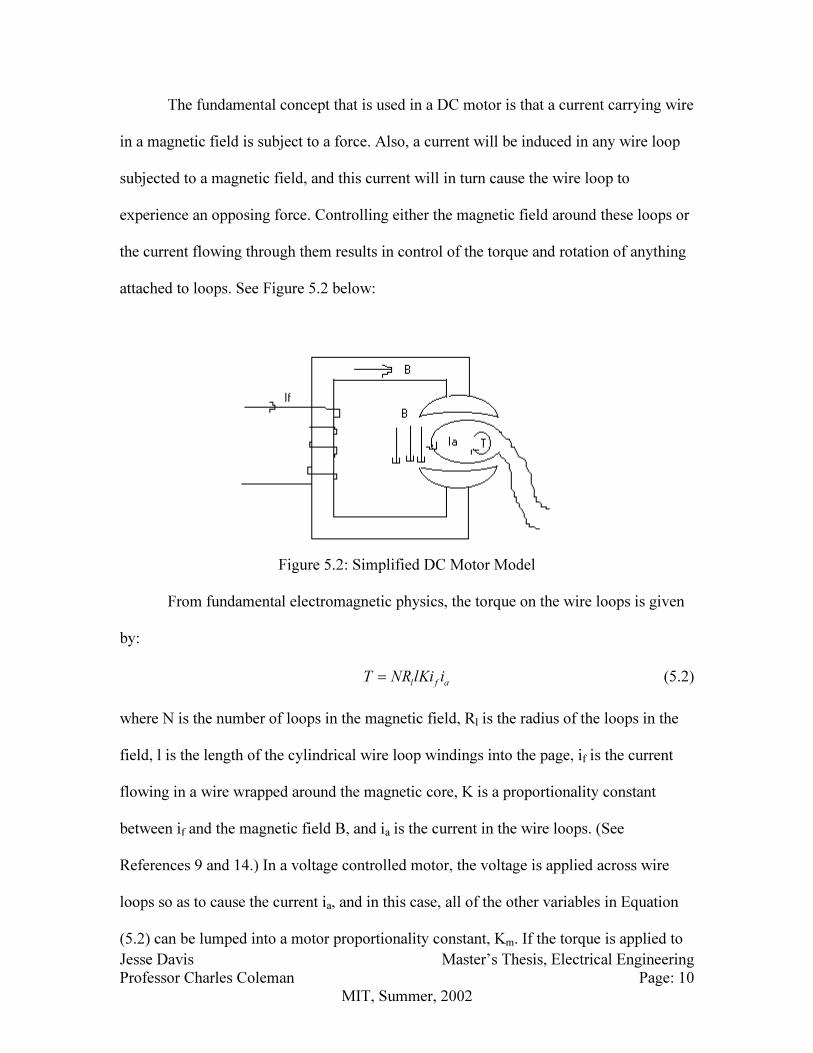
The fundamental concept that is used in a DC motor is that a current carrying wire
in a magnetic field is subject to a force. Also, a current will be induced in any wire loop
subjected to a magnetic field, and this current will in turn cause the wire loop to
experience an opposing force. Controlling either the magnetic field around these loops or
the current flowing through them results in control of the torque and rotation of anything
attached to loops. See Figure 5.2 below:
Figure 5.2: Simplified DC Motor Model
From fundamental electromagnetic physics, the torque on the wire loops is given
by:
l f aT NR lKi i= (5.2)
where N is the number of loops in the magnetic field, Rl is the radius of the loops in the
field, l is the length of the cylindrical wire loop windings into the page, if is the current
flowing in a wire wrapped around the magnetic core, K is a proportionality constant
between if and the magnetic field B, and ia is the current in the wire loops. (See
References 9 and 14.) In a voltage controlled motor, the voltage is applied across wire
loops so as to cause the current ia, and in this case, all of the other variables in Equation
(5.2) can be lumped into a motor proportionality constant, Km. If the torque is applied to
Jesse Davis Master’s Thesis, Electrical Engineering
Professor Charles Coleman Page: 11
MIT, Summer, 2002
some motor inertia, Im, plus some load inertia, Il, an angular speed, b, will result. The
relationship between torque and angular speed is given by:
( )m a m l
bT K i I I
t
∂= = +
∂ (5.3)
The motor itself can be modeled as a series connected inductance, L, and
resistance, RΩ
, and thus if a voltage, V, is across the motor terminals, the relationship
between the voltage and current ia will be:
a
a
iV i R L
tΩ
∂= +
∂ (5.4)
However, the applied voltage, Va, is not necessarily equal to the actual voltage, V, across
the motor due to the back voltage induced in the loops by the magnetic field. The back
voltage, Ve, is given by:
e e
V K b= (5.5)
Thus, Equation (5.4) should be re-written as:
a
a e a
iV V i R L
tΩ
∂− = +
∂ (5.6)
Combining Equations (5.3), (5.5), and (5.6), the full relationship between Va and b can be
seen to be:
( ) ( ) 2
2
m l m l
a e
m m
R I I L I Ib bV K
K t K t
Ω+ +∂ ∂
= + +∂ ∂
(5.7)
From Equation (5.7), it is simple to see that there are two states associated with a voltage
controlled motor, and in fact, for realistic motors, this is generally an over-damped
second order relationship.

Jesse Davis Master’s Thesis, Electrical Engineering
Professor Charles Coleman Page: 12
MIT, Summer, 2002
5.2.2 Craft-Based Three-Dimensional Translational Motion
The three-dimensional translational motion states are derived straight from
Newton’s Second Law of Motion:
2F m r=∑ (5.8)
The only translational forces on the craft result from the three propellers and gravity, so
the analysis here is quite straightforward. (The force of gravity will be included only in
the Earth-based reference in section 5.2.4. This choice is made in order that the reference
frames are not confused. In the Earth-based reference frame, the force of gravity is
always oriented on the negative z-axis, but in the craft based frame, the orientation is not
so clearly defined.) To slightly complicate matters, the propellers are tilted out of the
plane of the craft, by an angle ‘d’, in order to increase the torque around the out of plane
axis, thus increasing the hoop’s rotational speed. This out of plane tilt is depicted in
Figure 5.3 below:
Figure 5.3: Propeller Mounting Advance Angle
In order to create the equations of motion, a reference frame must be established.
The first reference frame that will be established is a craft-based reference frame, and in

Jesse Davis Master’s Thesis, Electrical Engineering
Professor Charles Coleman Page: 13
MIT, Summer, 2002
section 5.2.4, a translation between craft-based and Earth-based reference frames will be
developed. Figure 5.4 shows the orientation of the craft-based reference frame:
Figure 5.4: Craft-Based Reference Frame
Let the propeller depicted on the x-axis be propeller 1, the propeller immediately counter-
clockwise in the diagram be propeller 2, and the last propeller be propeller 3. The one
special feature about this reference frame is that it is completely fixed only to the hub and
not to the hoop, so the hoop can have a z-axis rotation in the reference frame. The angle
of rotation of the hoop in the craft-based reference frame will be defined as C
oψ .
From elementary thrust theory, the normal force exerted by a spinning propeller is
2 2 41
2
C
t propf C n b Rρ π= (5.9)
where the ‘C’ superscript denotes the force in a craft-based reference frame, Ct is the
propeller’s coefficient of thrust, ρ is the density of air, n is the gear ratio between the
propeller and the motor, b is the rotational speed of the motor (which is the same b as in
Equation (5.7)), and Rprop is the propeller radius. (See Reference 8.) From Figure 5.3, the
advance angle of the propellers is d, so the z-axis component of the forces from each of
the three propellers will be:
( )(1,2,3) (1,2,3) cosC C
zf f d= (5.10)

Jesse Davis Master’s Thesis, Electrical Engineering
Professor Charles Coleman Page: 14
MIT, Summer, 2002
The x- and y-axis components of the propeller forces, before any z-axis hoop rotation,
will be:
( )(1) (1) sin cos 0
2
C C
xf f d
π = =
(5.11)
( ) ( )(1) (1) (1)sin sin sin
2
C C C
yf f d f dπ
= =
(5.12)
( )(2) (2)
7sin cos
6
C C
xf f d
π =
(5.13)
( )(2) (2)
7sin sin
6
C C
yf f dπ
=
(5.14)
( )(3) (3)
11sin cos
6
C C
zf f d
π =
(5.15)
( )(3) (3)
11sin sin
6
C C
zf f d
π =
(5.16)
where the angles are measured from the x-axis counter-clockwise. (The angles are 2
π
ahead of the propeller locations at 0, 2
3
π
, and 4
3
π
.)
The state-equations in the craft-based reference frame are thus:
C
C
xC CC
y
C
C z
x
tv
s yv
t tv
z
t
∂ ∂
∂ ∂ = = ∂ ∂
∂ ∂
uur
(5.17)
1
C
Cvf
t m
∂=
∂
uur
uuur
(5.18)

Jesse Davis Master’s Thesis, Electrical Engineering
Professor Charles Coleman Page: 15
MIT, Summer, 2002
where C
xv , C
yv , and C
zv are the velocities of the craft along the x-, y-, and z- craft-based
axes, and Cfuuur
is specified by Equations (5.10)-(5.16) and rotated through C
oψ :
( ) ( )
( ) ( )
( )
( )
(1) (2) (3)
(1) (2) (3)
(1) (2) (3)
(1) (2) (3)
7 11sin cos cos cos
2 6 6cos sin 0
sin cos 0 sin
0 0 1
C C C C C C
o o oC C
C C Co o
x x x
C C C C C C
o o y y y
C C C
z z z
d f f f
f f f
f f f f d f
f f f
π π πψ ψ ψ
ψ ψ
ψ ψ
+ + + + +
− + + = + + = + +
uuur
( )( )
(1) (2) (3)
(1) (2) (3)
7 11sin sin sin
2 6 6
cos
C C C C C C
o o o
C C C
f f
d f f f
π π πψ ψ ψ
+ + + + +
+ +
(5.19)
5.2.3 Craft-Based Three-Dimensional Rotational Motion
As for the rotational motion of the craft in the craft-based reference frame, there
are four primary angles of concern. The angles that need to be tracked are the pitch, roll,
and yaw angles of the hoop, as well as the yaw angle of the hub. (The pitch and roll of the
hub are the same as for the hoop by construction.) Let the roll be an angle Cθ around the
x-axis, the pitch be an angle Cφ around the y-axis, the hoop yaw be an angle C
oψ around
the z-axis, and the hub yaw be an angle C
iψ around the z-axis. Furthermore, let
C
C
tθ
θω
∂=
∂ (5.20)
C
C
tφ
φω
∂=
∂ (5.21)
o
C
Co
tψ
ψω
∂=
∂ (5.22)
i
C
Ci
tψ
ψω
∂=
∂ (5.23)

Jesse Davis Master’s Thesis, Electrical Engineering
Professor Charles Coleman Page: 16
MIT, Summer, 2002
be the rotational velocities of the hoop around the x-, y-, and z-axes and the hub around
the z-axis. These last four equations also make up the first four rotational motion state
equations.
From Euler’s laws of angular motion it is known that:
M J Jt
ω
ω ω
∂= + ×
∂∑ (5.24)
where M are the moment vectors, J is a moment of inertia matrix, and ω is the vectored
angular velocity. This leads to state equations for rotational motion of:
( )1J M J
t
ω
ω ω−
∂= − ×
∂∑ (5.25)
This equation will have two parts to it, the first to deal with the hub and the second to
deal with the hoop. All variables for the hub will have a subscript ‘i’, and all variables for
the outer hub will have a subscript ‘o’. With a rigid-body assumption, and thus entirely
independent axes of motion, the moment of inertia matrices are given by:
0 0
0 0
0 0i
xx
i yy
zz
I
J I
I
=
(5.26)
and
0 0
0 0
0 0o
xx
o yy
zz
I
J I
I
=
(5.27)
The two different ω vectors are given by:
i
C
C C
i
C
θ
φ
ψ
ω
ω ω
ω
=
uuur
(5.28)

Jesse Davis Master’s Thesis, Electrical Engineering
Professor Charles Coleman Page: 17
MIT, Summer, 2002
and
o
C
C C
o
C
θ
φ
ψ
ω
ω ω
ω
=
uuur
(5.29)
The moments that will be exerted on the craft will have three different sources:
one from the changing rotational velocities of the propellers, another from the torque
exerted on the craft by the forces caused by the propellers, and another from the yaw
motor’s changing rotational velocity. Moments from the first source will be labeled with
a subscript ‘1’, from the second source ‘2’, and the third source ‘3’. Since the x- and y-
axis rotational motion of the hoop and hub are locked together, the x- and y- components
of all of the moments will act on both the hoop and hub as if they are one body.
Additionally, the x- and y-axis rotational state equations for the hoop and hub must be the
same. Since the z-axis rotational motion of the hoop and hub can be different, however,
care must be taken to specify which sections of the craft each of the z-axis moments will
act on.
The z-axis component of the moments from the first and second sources will act
only on the hoop. The reason for this is that the source of these moments is from bodies
connected only to the hoop, namely the motors and propellers. The z-axis component of
the moment from the third source will act on both the hoop and the hub, however. This is
because the yaw motor will be connected to both sections of the craft, and will therefore
affect both sections. These precise effects will be discussed shortly.
As for the actual equations, the moment caused by the first source, the changing
rotational velocities of the propellers, will be:

Jesse Davis Master’s Thesis, Electrical Engineering
Professor Charles Coleman Page: 18
MIT, Summer, 2002
( ) ( )
( ) ( )
( ) ( )
(1)
(1)
1(1)
(1)
sin cos2
sin sin2
cos
C
m p o
C C
m p o
m p
bI nI d
t
bM I nI d
t
bI nI d
t
πψ
πψ
∂ + + ∂
∂ = + +
∂ ∂
+ ∂
uuuuur
(5.30)
( ) ( )
( ) ( )
( ) ( )
(2)
(2)
1(2)
(2)
7sin cos
6
7sin sin
6
cos
C
m p o
C C
m p o
m p
bI nI d
t
bM I nI d
t
bI nI d
t
πψ
πψ
∂ + + ∂
∂ = + +
∂ ∂
+ ∂
uuuuur
(5.31)
( ) ( )
( ) ( )
( ) ( )
(3)
(3)
1(3)
(3)
11sin cos
6
11sin sin
6
cos
C
m p o
C C
m p o
m p
bI nI d
t
bM I nI d
t
bI nI d
t
πψ
πψ
∂ + + ∂
∂ = + +
∂ ∂
+ ∂
uuuuur
(5.32)
for motors (1), (2), and (3), giving a total of:
( ) ( )
( ) ( )
( ) ( )
(1) (2) (3)
(1) (2) (3)
1
(1)
7 11sin cos cos cos
2 6 6
7 11sin sin sin sin
2 6 6
cos
C C C
m p o o o
C C C C
m p o o o
m p
b b bI nI d
t t t
b b bM I nI d
t t t
bI nI d
t
π π πψ ψ ψ
π π πψ ψ ψ
∂ ∂ ∂ + + + + + +
∂ ∂ ∂
∂ ∂ ∂ = + + + + + +
∂ ∂ ∂
∂+
∂
uuuur
(2) (3)b b
t t
∂ ∂ + + ∂ ∂
(5.33)
where Im is the moment of inertia of the motor and motor gear, and Ip is the moment of
inertia of the propeller and propeller gear.
The moments from the second source, the torque from the forces caused by the
propellers, will all take the form:

Jesse Davis Master’s Thesis, Electrical Engineering
Professor Charles Coleman Page: 19
MIT, Summer, 2002
2(1,2,3) (1,2,3) (1,2,3)
C C CM r f= ×
uuuuuuuur uuuuur uuuuuur
(5.34)
The forces have already been defined, but the position vectors for the motors, (1,2,3)
Cr
uuuuur
, have
not yet been determined. From Figure 5.4, the position of the motors is apparent:
( )
( )(1)
cos
sin
0
C
m o
C C
m o
R
r R
ψ
ψ
=
uur
(5.35)
(2)
2cos
3
2sin
3
0
C
m o
C C
m o
R
r R
πψ
πψ
+
= +
uur
(5.36)
(3)
4cos
3
4sin
3
0
C
m o
C C
m o
R
r R
πψ
πψ
+
= +
uur
(5.37)
where Rm is the radius from the hub center to propeller center. Using Equation (5.34) to
combine Equations (5.10)-(5.16) and (5.35)-(5.37), the total moment from the second
source is:
( ) ( )
( ) ( )
( ) ( )
(2) (2) (3)
2 (1) (2) (3)
(1) (2) (3)
2 4cos sin sin sin
3 3
2 4cos cos cos cos
3 3
sin sin2
C C C C C C
m o o o
C C C C C C C
m o o o
C C C
m
R d f f f
M R d f f f
R d f f f
π πψ ψ ψ
π πψ ψ ψ
π
+ + + +
= − + + + +
+ +
uuuur
(5.38)

Jesse Davis Master’s Thesis, Electrical Engineering
Professor Charles Coleman Page: 20
MIT, Summer, 2002
Lastly, the moment caused by the third source, the yaw motor’s changing
rotational velocity, will be a positive moment for the hoop and a negative moment for the
hub. This orientation is chosen so that the yaw motor will counter-act the frictional forces
between the hub and hoop which would tend to draw the hub into a rotation with the
hoop. Since the hub needs to be de-spun in order to mount an effective autopilot on it, the
yaw motor must counter-balance this pull. The moment from the yaw motor on the hoop
will be:
( )
3
,
0
0o
o i
C
yaw
m yaw zz zz
M
bI I I
t
= ∂ + + ∂
uuuur
(5.39)
and correspondingly on the hub will be:
( )
3
,
0
0i
o i
C
yaw
m yaw zz zz
M
bI I I
t
= − ∂ + + ∂
uuuur
(5.40)
where Im,yaw is the moment of inertia associated with the yaw motor.
Combining all the moments of Equations (5.33), (5.38), (5.39), and (5.40), the
total moment on the hoop will be:

Jesse Davis Master’s Thesis, Electrical Engineering
Professor Charles Coleman Page: 21
MIT, Summer, 2002
( ) ( )
( ) ( )
( ) ( )
(1) (2) (3)
(1) (2) (3)
(1)
7 11sin cos cos cos
2 6 6
7 11sin sin sin sin
2 6 6
cos
C C C
m p o o o
C C C C
o m p o o o
m p
b b bI nI d
t t t
b b bM I nI d
t t t
bI nI d
t
π π πψ ψ ψ
π π πψ ψ ψ
∂ ∂ ∂ + + + + + +
∂ ∂ ∂
∂ ∂ ∂ = + + + + + +
∂ ∂ ∂
∂+
∂
uuuur
( )(2) (3)
,o i
yaw
m yaw zz zz
b b bI I I
t t t
∂ ∂ ∂ + + + + + ∂ ∂ ∂
( ) ( )
( ) ( )
( ) ( )
(1) (2) (3)
(1) (2) (3)
(1) (2) (3)
2 4cos sin sin sin
3 3
2 4cos cos cos cos
3 3
sin sin2
C C C C C C
m o o o
C C C C C C
m o o o
C C C
m
R d f f f
R d f f f
R d f f f
π πψ ψ ψ
π πψ ψ ψ
π
+ + + + +
− + + + +
+ + +
(5.41)
where the x- and y-components act on both the hoop and hub, and the z-component acts
only on the hoop. The total z-component moment that acts on the hub is given by
Equation (5.40).
Now that the total moment on each section of the craft is established, Equations
(5.25)-(5.29) can be used to finally derive the state equations for C
iω
uuur
and C
oω
uuur
. However,
a transformation will have to be developed between the rotational velocities in a rotated
hoop-based frame, r
iω
uur
and r
oω
uur
, and an un-rotated hub-based frame, C
iω
uuur
and C
oω
uuur
. (The
only difference between the rotated and un-rotated craft-based frames is that the rotated
craft-based frame is rigidly attached to the hoop, while the un-rotated craft-based frame is
rigidly attached to the hub.) The rotated craft-based frame will have rotational velocities
of:
Jesse Davis Master’s Thesis, Electrical Engineering
Professor Charles Coleman Page: 22
MIT, Summer, 2002
( ) ( ) ( )
( ) ( )( )
( )
(2) (3)
(1) (2) (3)
1 7 11sin cos cos
6 6
1 7 11sin sin sin
6 6
1
o o
o o
i
C C
yy zz m p
xx
rC Ci
zz xx m p
yy
C C
xx yy
zz
b bI I d I nI
I t t
b b bI I d I nI
t I t t t
I II
φ ψ
θ ψ
θ φ
π π
ω ω
ω π π
ω ω
ω ω
∂ ∂ − + + +
∂ ∂
∂ ∂ ∂ ∂ = − + + + +
∂ ∂ ∂ ∂
−
uur
( ),o i
yaw
m yaw zz zz
bI I I
t
∂
− + + ∂
( )
( )
(2) (3)
(1) (2) (3)
1 2 4cos sin sin
3 3
1 2 4cos cos cos
3 3
0
C C
m
xx
C C C
m
yy
R d f fI
R d f f fI
π π
π π
+ +
− + +
+
(5.42)
( ) ( )( )
( ) ( )( )
( )
(2) (3)
(1) (2) (3)
1 7 11sin cos cos
6 6
1 7 11sin sin sin
6 6
1
o o
o o
i
C C
yy zz m p
xx
rC Co
zz xx m p
yy
C C
xx yy
zz
b bI I d I nI
I t t
b b bI I d I nI
t I t t t
I II
φ ψ
θ ψ
θ φ
π π
ω ω
ω π π
ω ω
ω ω
∂ ∂ − + + +
∂ ∂
∂ ∂ ∂ ∂ = − + + + +
∂ ∂ ∂ ∂
−
uur
( ) ( )( ) (1) (2) (3)
, coso i
yaw
m yaw zz zz m p
b b b bI I I d I nI
t t t t
∂ ∂ ∂ ∂
+ + + + + + + ∂ ∂ ∂ ∂
( )
( )
( ) ( )
(2) (3)
(1) (2) (3)
(1) (2) (3)
1 2 4cos sin sin
3 3
1 2 4cos cos cos
3 3
1sin sin
2o
C C
m
xx
C C C
m
yy
C C C
m
zz
R d f fI
R d f f fI
R d f f fI
π π
π π
π
+ +
− + +
+ + +
(5.43)
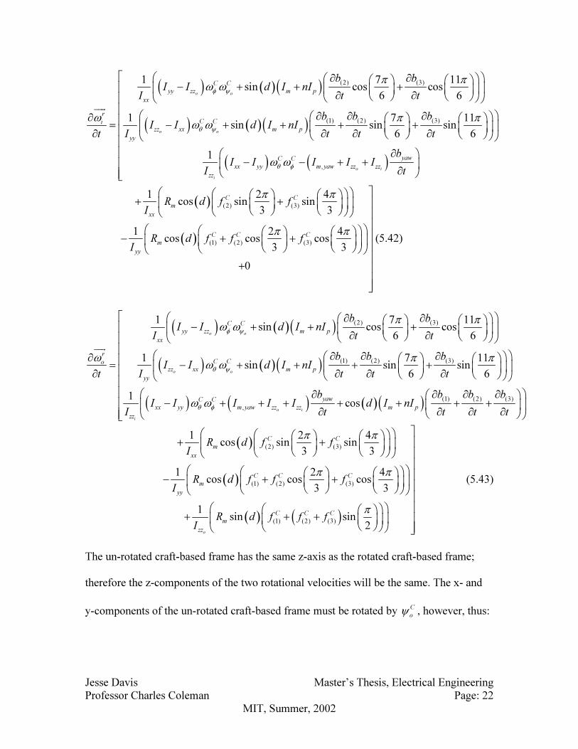
The un-rotated craft-based frame has the same z-axis as the rotated craft-based frame;
therefore the z-components of the two rotational velocities will be the same. The x- and
y-components of the un-rotated craft-based frame must be rotated by C
oψ , however, thus:

Jesse Davis Master’s Thesis, Electrical Engineering
Professor Charles Coleman Page: 23
MIT, Summer, 2002
( ) ( )
( ) ( ),
,
cos sin 00
0 sin cos 0
00 0 1i o
C CC
o ox
r C C C
i o o o y
C
z
ψ ψω
ω ψ ψ ω
ω
− = +
uuur
(5.44)
Solving for ,
C
i oω
uuur
gives:
( ) ( )
( ) ( ), ,
cos sin 0
sin cos 0
0 0 1
C C
o o
C C C r
i o o o i o
ψ ψ
ω ψ ψ ω
= −
uuur uuur
(5.45)
which is simply the rotated rotational velocity multiplied by an inverse rotation of C
oψ .
The full form of ,
C
i oω
uuur
is omitted to conserve space.
5.2.4 Earth-Based Three-Dimensional Translational and Rotational Motion
Now that the craft-based reference frame has been fully understood, a conversion
between the craft-based frame and an Earth-based frame must be established. The three
major differences between the craft-based frame and the Earth-based frame are the
difference in origin, the difference in rotational orientation, and the addition of a constant
z-axis force of gravity in the Earth-based frame. The difference in origin is very easy to
add in since it is simply a translational offset and will not affect the state equations at all.
Also, the force of gravity is easy to add in since it is simply a constant z-directed force.
The most difficult conversion is that of the rotation angles.
Let Eθ be the Earth-based x-axis angle, Eφ be the Earth-based y-axis angle, E
iψ
be the Earth-based z-axis angle relating to the hub, and E
oψ be the Earth-based z-axis
angle relating to the hoop. If the translational offset is subtracted from the craft-based
reference frame, these angles are those through which the craft-based frame would have
Jesse Davis Master’s Thesis, Electrical Engineering
Professor Charles Coleman Page: 24
MIT, Summer, 2002
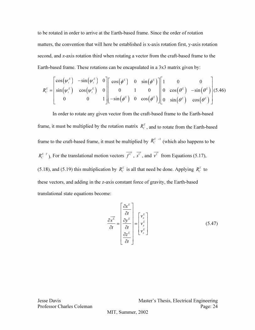
to be rotated in order to arrive at the Earth-based frame. Since the order of rotation
matters, the convention that will here be established is x-axis rotation first, y-axis rotation
second, and z-axis rotation third when rotating a vector from the craft-based frame to the
Earth-based frame. These rotations can be encapsulated in a 3x3 matrix given by:
( ) ( )
( ) ( )( ) ( )
( ) ( )( ) ( )
( ) ( )
cos sin 0 cos 0 sin 1 0 0
sin cos 0 0 1 0 0 cos sin
sin 0 cos0 0 1 0 sin cos
E E E Ei i
E E E E E
C i i
E EE E
R
ψ ψ φ φ
ψ ψ θ θ
φ φ θ θ
− = −
−
(5.46)
In order to rotate any given vector from the craft-based frame to the Earth-based
frame, it must be multiplied by the rotation matrix E
CR , and to rotate from the Earth-based
frame to the craft-based frame, it must be multiplied by 1E
CR
−
(which also happens to be
E T
CR ). For the translational motion vectors Cf
uuur
, Cs
uur
, and Cv
uur
from Equations (5.17),
(5.18), and (5.19) this multiplication by E
CR is all that need be done. Applying E
CR to
these vectors, and adding in the z-axis constant force of gravity, the Earth-based
translational state equations become:
E
E
xE EE
y
E
E z
x
tv
s yv
t tv
z
t
∂ ∂
∂ ∂ = = ∂ ∂
∂ ∂
uur
(5.47)

Jesse Davis Master’s Thesis, Electrical Engineering
Professor Charles Coleman Page: 25
MIT, Summer, 2002
( ) ( ) ( ) ( ) ( ) ( ) ( )( ) ( ) ( ) ( )
( ) ( ) ( ) ( ) ( ) ( ) ( )( )
(1) (2) (3) (1) (2) (3)
(1) (2) (3) (1) (2)
7 11c
2 6 6
1 7c
2 6
C C C E E E E E C C C C C C E E
i i o o o i
E
C C C E E E E E C C C C
i i o o
f f f d c s c s s f c f c f c s d c c
vf f f d s s c c s f c f c
t m
π π πψ φ θ ψ θ ψ ψ ψ ψ φ
π πψ φ θ ψ θ ψ ψ
+ + + + + + + + +
∂ = + + − + + + + +
∂
uur
( ) ( ) ( )
( ) ( ) ( ) ( ) ( ) ( )
(3)
(1) (2) (3) (1) (2) (3)
11
6
7 11c
2 6 6
C C E E
o i
C C C E E C C C C C C E
o o o
f c s d s c
gm f f f d c c f c f c f c s d s
πψ ψ φ
π π πφ θ ψ ψ ψ φ
+
− + + + − + + + + +
( ) ( ) ( ) ( ) ( ) ( )( )
( ) ( ) ( ) ( ) ( ) ( )( )
(1) (2) (3)
(1) (2) (3)
(1) (2)
7 11
2 6 6
7 11
2 6 6
7
2
C C C C C C E E E E E
o o o i i
C C C C C C E E E E E
o o o i i
C C C
o
f s f s f s s d c s s s c
f s f s f s s d s s s c c
f s f s
π π πψ ψ ψ ψ φ θ ψ θ
π π πψ ψ ψ ψ φ θ ψ θ
π πψ
+ + + + + + −
+ + + + + + +
+ + +
( ) ( ) ( )(3)
11
6 6
C C C E E
o of s s d c s
πψ ψ φ θ
+ + +
(5.48)
where the shorthand c(*) replaces cos(*) and s(*) replaces sin(*), g is the acceleration
due to gravity, and m is the craft’s total mass. The z-axis angle of the hub is used since it
is ultimately the orientation of the hub which will be controlled, and also since the craft-
based reference frame is really a hub-based reference frame.
As for the rotational motion, by association with Equations (5.20)-(5.23), the first
rotational motion state equations in the Earth-based frame are:
E
E
tθ
θω
∂=
∂ (5.49)
E
E
tφ
φω
∂=
∂ (5.50)
o
E
Eo
tψ
ψω
∂=
∂ (5.51)
i
E
Ei
tψ
ψω
∂=
∂ (5.52)
The conversion of the rotational velocity vectors from the craft-based frame to the Earth-
based frame is slightly more complicated than for the translational motion. The same

Jesse Davis Master’s Thesis, Electrical Engineering
Professor Charles Coleman Page: 26
MIT, Summer, 2002
rotation that was applied to the translational vectors cannot be applied again. The reason
for this is that the rotational axes must be separated from each other in order to correctly
convert their components. If the order of rotation is x-axis, y-axis, z-axis when rotating
from the craft-based frame to the Earth-based frame, then the x-axis component of ,
E
i oω
uuur
will be the same as the x-axis component of ,
C
i oω
uuur
. However, the y-axis component of ,
E
i oω
uuur
must be un-rotated through the x-axis Earth-based rotation angle, and the z-axis
component of ,
E
i oω
uuur
must be un-rotated through both the x- and y-axis Earth-based rotation
angles. The conversion becomes:
( ) ( )
( ) ( )
( ) ( )
( ) ( )
( ) ( )
( ) ( ),
,
cos 0 sin1 0 0 1 0 00 0
0 0 cos sin 0 cos sin 0 1 0 0
0 0 sin 0 cos0 sin cos 0 sin cos i o
E EE
C E E E E E
i o
EE EE E E E
θ
φ
ψ
φ φω
ω θ θ ω θ θ
ωφ φθ θ θ θ
− = + + − −
uuur
(5.53)
giving
( )
( ) ( ) ( )
( ) ( ) ( )
, ,
1 0 sin
0 cos cos sin
0 sin cos cos
E
C E E E E
i o i o
E E E
φ
ω θ φ θ ω
θ φ θ
− = −
uuur uuur
(5.54)
Solving Equation (5.54) for ,
E
i oω
uuur
gives:
( ) ( ) ( ) ( )
( ) ( )
( )( )
( )( )
, ,
1 tan sin tan cos
0 cos sin
sin cos0
cos cos
E E E E
E E E C
i o i o
E E
E E
φ θ φ θ
ω θ θ ω
θ θ
φ φ
= −
uuur uuur
(5.55)

Jesse Davis Master’s Thesis, Electrical Engineering
Professor Charles Coleman Page: 27
MIT, Summer, 2002
By this equation, there will be two different E
xω and E
yω , one for the hub and one for the
hoop. The E
xω and E
yω that will be concentrated on are those for the hub. This is done
because it is ultimately the orientation of the hub that will be controlled, so knowing its
rotational velocities is of primary importance. Finally, the complete state-space
description of the craft in both the craft-based and Earth-based reference frames has been
shown.
5.3 Altitude, Attitude, and Yaw Control
The actual implementation of the craft and user interface is going to take the form
of a two joystick remote control mechanism that can operate in two separate modes. In a
user controlled mode, one joystick will control roll and pitch, and the other will control
yaw motor speed and thrust; in a computer controlled mode, one joystick will control roll
and pitch, and the other will control yaw speed of the hub and vertical speed. In the
computer controlled mode, the user’s commands will be processed by a controller so that
the on-board computer ultimately controls the craft. To this end, three essentially separate
motions will need to be controlled: vertical speed, yaw speed of the hub, and attitude
(pitch and roll).
5.3.1 System Analysis
5.3.1.1 Motor Voltages and Forces
The yaw speed control is essentially separated from the other two controlled
dynamics because the yaw motor is the main actuator of craft-based z-axis torque. From
Equation (5.42) and (5.45):
( ) ( ),
1z
i o
i
C
i yawC C
xx yy m yaw zz zz
zz
bI I I I I
t I tθ φ
ω
ω ω
∂ ∂ = − − + +
∂ ∂ (5.56)

Jesse Davis Master’s Thesis, Electrical Engineering
Professor Charles Coleman Page: 28
MIT, Summer, 2002
Since Ixx ~ Iyy, and also since C
θω ~ C
φω ~ 0 around any stable operating point for which
we are designing the controller, it is clear that the moment imparted by the yaw motor is
dominant. Furthermore, the yaw motor moment doesn’t appear in either the x- or y-axis
component of ,
C
i oω
uuur
; hence the yaw control can be fully actuated with the yaw motor alone
while not affecting any other aspect of the craft.
The reason the altitude and attitude control are essentially independent requires
more development. Since the three propellers will provide both lift and steering of the
craft, it initially does not seem reasonable that the altitude and attitude control can be
separated. The method by which the motors provide lift is quite obvious; if higher
voltages are applied to the motors, the motors will turn the propellers faster, the
propellers will provide more lift, and the craft will rise along its z-axis. (As well as spin
slightly faster around its z-axis due to the advance angle d.) In order to steer the craft,
however, it seems reasonable that different voltages will have to be applied to each
motor. In addition, since the motors are rotating along with the rest of the hoop, these
voltages will have to be adjusted depending on the yaw of the hoop.
In order to steer the craft, some torque vector in the craft-based x-y plane will
have to be created around which the craft will then pivot. Looking at Equations (5.42)
and (5.43) again, noting that the rotation of Equation (5.45) will linearly combine x- and
y-components, and assuming that the advance angle of the propellers, d, will be small, the
primary components of the x- and y-axis moments are due to forces exerted by the
propellers at certain lever arms away from the origin. As an engineering assumption,
these torques will be considered the dominant torques experienced by the craft along its
x- and y-axes, and so these are the torques that will be controlled in order to steer the
Jesse Davis Master’s Thesis, Electrical Engineering
Professor Charles Coleman Page: 29
MIT, Summer, 2002
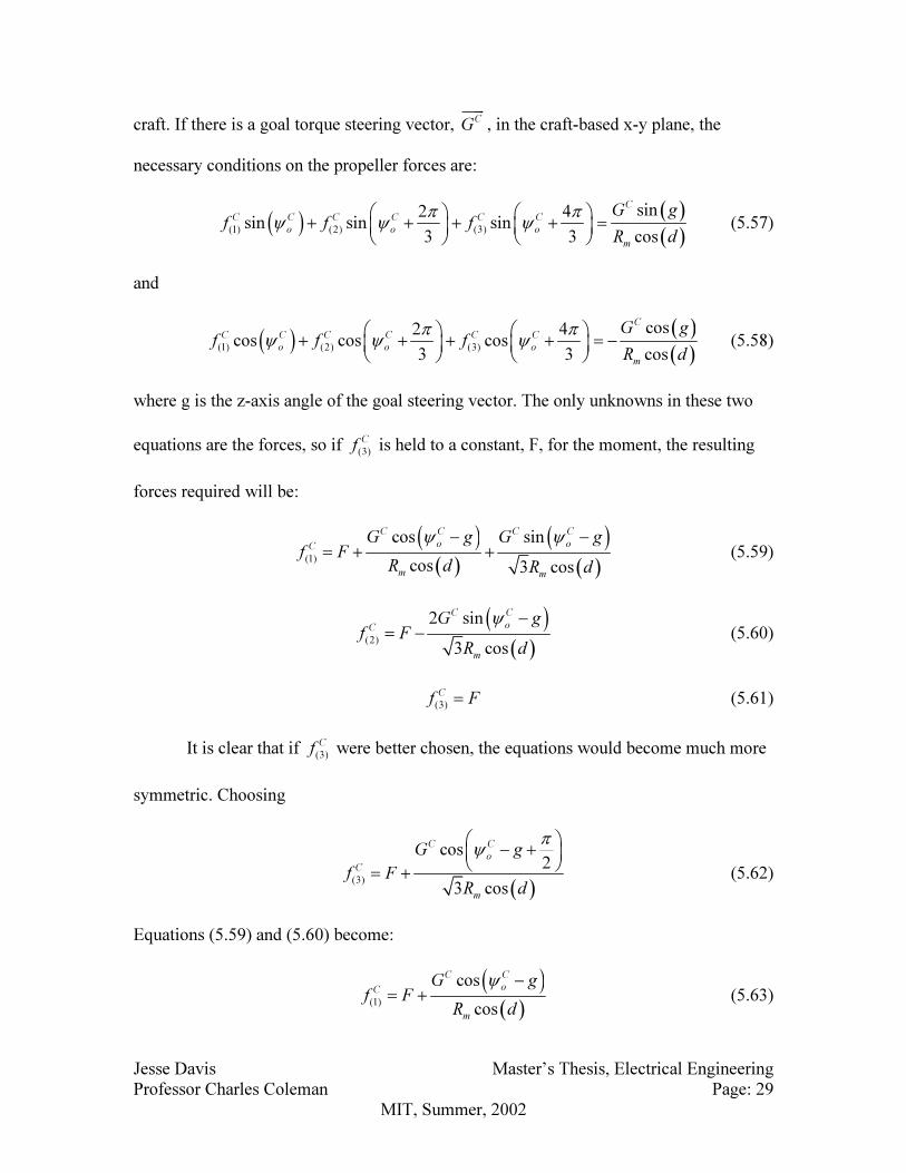
craft. If there is a goal torque steering vector, CG
uuur
, in the craft-based x-y plane, the
necessary conditions on the propeller forces are:
( )( )
( )(1) (2) (3)
sin2 4sin sin sin
3 3 cos
C
C C C C C C
o o o
m
G gf f f
R d
π πψ ψ ψ
+ + + + =
(5.57)
and
( )( )
( )(1) (2) (3)
cos2 4cos cos cos
3 3 cos
C
C C C C C C
o o o
m
G gf f f
R d
π πψ ψ ψ
+ + + + = −
(5.58)
where g is the z-axis angle of the goal steering vector. The only unknowns in these two
equations are the forces, so if (3)
Cf is held to a constant, F, for the moment, the resulting
forces required will be:
( )
( )
( )( )
(1)
cos sin
cos 3 cos
C C C C
o oC
m m
G g G gf F
R d R d
ψ ψ− −
= + + (5.59)
( )( )
(2)
2 sin
3 cos
C C
oC
m
G gf F
R d
ψ −
= − (5.60)
(3)
Cf F= (5.61)
It is clear that if (3)
Cf were better chosen, the equations would become much more
symmetric. Choosing
( )
(3)
cos2
3 cos
C C
o
C
m
G g
f FR d
πψ
− + = + (5.62)
Equations (5.59) and (5.60) become:
( )( )(1)
cos
cos
C C
oC
m
G gf F
R d
ψ −
= + (5.63)

Jesse Davis Master’s Thesis, Electrical Engineering
Professor Charles Coleman Page: 30
MIT, Summer, 2002
( )
(2)
cos2
3 cos
C C
o
C
m
G g
f FR d
πψ
− − = + (5.64)
where F is a thrust offset and is chosen such that the forces are never negative:
( )cos
C
m
GF
R d≥ (5.65)
Since Equation (5.9) gives a relationship between propeller thrust and motor rotational
speed, and Equation (5.7) gives a relationship between motor rotational speed and applied
voltage, the voltages that need to be applied to the motors in order to steer the craft can
be determined.
In Equation (5.7) there are three terms, one is a multiple of b, one is a multiple of
b
t
∂
∂, and one is a multiple of
2
2
b
t
∂
∂. Looking at the coefficients of these terms, it is clear
that the 2
2
b
t
∂
∂ can be neglected since a motor’s inductance will be at least three orders of
magnitude less than its resistance. The b
t
∂
∂ term cannot necessarily be neglected,
however. Motor’s have an intrinsic mechanical time constant associated with the spin up
of the rotor once a voltage is applied, and for the simple model developed in 5.2.1, this
time constant is given by:
( )m p
e m
R I nI
K Kτ
Ω+
= (5.66)
If this time constant is fast enough, and the hoop’s rotation is slow enough, the rotor’s
rotational speed can track the applied voltage without delay, and hence the b
t
∂
∂ term may

Jesse Davis Master’s Thesis, Electrical Engineering
Professor Charles Coleman Page: 31
MIT, Summer, 2002
be neglected. If the motor time constant is too slow, however, there will be an effective
time lag between the applied voltage sinusoid and the rotor’s rotational speed sinusoid
required to precisely steer the craft. This time lag can be interpreted as an angular lag if
o
C
ψω is known, and so the steering will always actually occur at a constant angle offset
from the commanded steering.
In order to find this angular offset, Equation (5.7) must be manipulated. First, the
2nd
order term is ignored as concluded in the paragraph above. Second, the Fourier
transform of the equation is taken giving:
1/
1
f
e
f
a
Kb
V iωτ=
+
(5.67)
where i equals 1− , the superscript ‘f’ denotes a Fourier transform variable, and ω is
the Fourier transform frequency. The phase delay, pd, of this equation at a frequency of
o
C
ψω is given by:
( )arctan
o
o
C
d Cp
ψ
ψ
τω
ω= (5.68)
which translates into an angular delay, o
ψδ , of:
( )arctano o
C
ψ ψδ τω= (5.69)
The last thing that needs to be determined is the amplitude change between Va
and b. This will simply be the magnitude of Equation (5.67) which is given by:
( )2
1/
1C
oo
f
e
fCa
Kb
Vψ
ωψ
ω τ
=
+
(5.70)

Jesse Davis Master’s Thesis, Electrical Engineering
Professor Charles Coleman Page: 32
MIT, Summer, 2002
Using Equations (5.9), (5.62)-(5.64), (5.69), and (5.70), the required applied voltages in
order to steer the craft to some goal torque CG
uuur
are:
( )( ) ( )( )
2
(1) 2 4
2 1 cos
cos
o
o
C C C
o
a e
t prop m
G gV K F
C n R R d
ψψ
ω τ ψ δ
ρ π
+− +
= + (5.71)
( )( )( )
2
(2) 2 4
cos2 12
3 cos
oo
C CCo
a e
t prop m
G g
V K FC n R R d
ψψ
πψ δω τ
ρ π
− + −+
= + (5.72)
( )( )( )
2
(3) 2 4
cos2 12
3 cos
oo
C CCo
a e
t prop m
G g
V K FC n R R d
ψψ
πψ δω τ
ρ π
− + ++
= + (5.73)
It is clear that each of these equations has three quantities which must be specified
in order for the craft to be manipulated: F, the force offset, GC, the goal torque
magnitude, and g, the goal torque angle. As was seen through the development of these
equations, the force offset F, does not affect the steering torque in any way. For any value
of F, if GC and g remain constant, the resulting torque will always be C
G
uuur
. (In the case if
the radicand of the second radical were to go negative, the radical should be taken of the
absolute value of the radicand, and a negative sign should be appended to the entire
equation. This would correspond to rotating the propellers in the direction opposite to
normal.)
The other part that is of concern is whether or not the total force in the z-direction
is independent of GC and g. Adding together Equations (5.62)-(5.64), the total force is:
( )( )
( )
cos
3cos
o
C C
oC
i
i m
G gf F
R d
ψψ δ− +
= +∑ (5.74)

Jesse Davis Master’s Thesis, Electrical Engineering
Professor Charles Coleman Page: 33
MIT, Summer, 2002
which is obviously not independent of GC or g. However, if the average of Equation
(5.74) is taken over a full cycle of C
oψ , the resultant average force is:
( ) 3C
o
C
i
i
f Fψ
=∑ (5.75)
which is, of course, independent of GC and g. Controlling the average force will be
sufficient as long as the actual vertical movement variation is not significant throughout a
rotation. Using only the z-component of Newton’s Second Law of Motion from Equation
(5.8), solving the differential equation for the z-position gives:
( )( )
2
2
1 2
cos3
2 cos
o
o
C C
o
C
m
G gFz t c t c
m mR d
ψ
ψ
ψ δ
ω
− +
= + + − (5.76)
if o
C
ψω is assumed to be a constant, where c1 and c2 are arbitrary integration constants.
Thus, as long as
( )
2
coso
C
C
m
G
mR dψ
ω (5.77)
the variation in z-position will be minimal. In order to satisfy this constraint, the craft
must be heavy, the steering cannot be too forceful, and the rotation rate of the craft must
be high. Plugging some likely numbers into this equation, it is not hard to see that this
constraint can easily be met. (Likely numbers are o
C
ψω ~ 10π, m ~ 1, Rm ~ .2, G
C <~1, and
d ~ 5 degrees.)
In the previous paragraphs it has been determined that F and CG
uuur
are essentially
independent of each other. Furthermore, 3F has been shown to be the primary vertical
force acting on the craft , and C
G
uuur
has been shown to be the primary craft-based x-y plane

Jesse Davis Master’s Thesis, Electrical Engineering
Professor Charles Coleman Page: 34
MIT, Summer, 2002
torque acting on the craft. Since F and C
G
uuur
can be independently set, the vertical motion
and rotational motion are de-coupled from each other. The proposition that the altitude
and attitude can be independently controlled has thus been proven.
5.3.1.2 Pitch, Roll, and Yaw
In order to steer the craft, a pitch, roll, yaw sensor will be placed on the hub. For
any given attitude, the sensor will give a constant reading, and for any given reading, the
craft must be at a given attitude. Since the order of rotation in rotation matrices matters,
so that a single Eθ , Eφ , and
,
E
i oψ combination can give rise to six different attitudes
depending on what order the rotations are made in, the question arises as to what the
sensor is actually measuring. Furthermore, there is another question as to how to translate
between the rotation matrix angles, Eθ , Eφ , and E
iψ , and the sensor’s pitch, roll, and
yaw measurements, E
mθ , E
mφ , and
i
E
mψ . (The subscript ‘m’ will denote a measured
variable.) It is in fact the sensor’s measured angles that will be controlled, and not the
Earth-based rotation matrix angles. This will make any combination of angles unique to a
given attitude so there can be no confusion about the orientation of the craft at any time.
The sensor assumes there is a front end of the craft and a vector which points
from the center of the craft through the front, and also from the center of the craft straight
up. For the purpose of this discussion, it is assumed that before any rotation, the front
pointing vector is co-linear with the Earth-based x-axis, and the up pointing vector (the
normal vector) is co-linear with the Earth-based z-axis. To follow this discussion, Figure
5.5 below will help with orientation.
Jesse Davis Master’s Thesis, Electrical Engineering
Professor Charles Coleman Page: 35
MIT, Summer, 2002
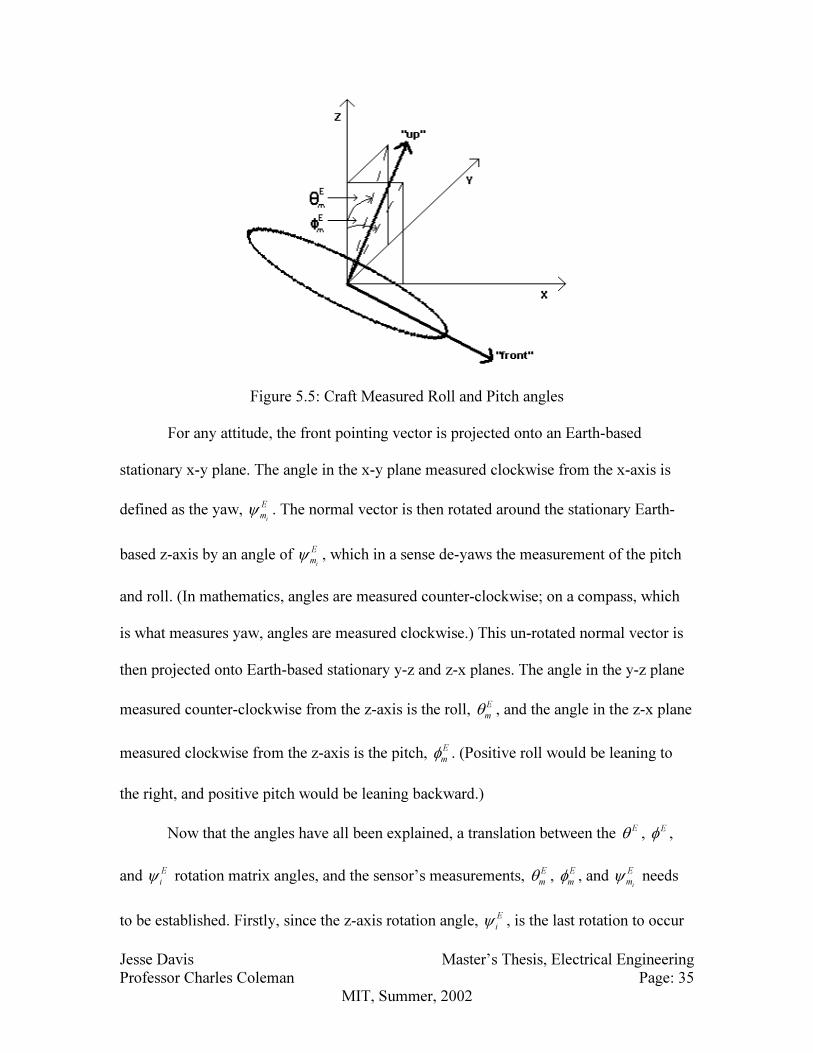
Figure 5.5: Craft Measured Roll and Pitch angles
For any attitude, the front pointing vector is projected onto an Earth-based
stationary x-y plane. The angle in the x-y plane measured clockwise from the x-axis is
defined as the yaw, i
E
mψ . The normal vector is then rotated around the stationary Earth-
based z-axis by an angle of i
E
mψ , which in a sense de-yaws the measurement of the pitch
and roll. (In mathematics, angles are measured counter-clockwise; on a compass, which
is what measures yaw, angles are measured clockwise.) This un-rotated normal vector is
then projected onto Earth-based stationary y-z and z-x planes. The angle in the y-z plane
measured counter-clockwise from the z-axis is the roll, E
mθ , and the angle in the z-x plane
measured clockwise from the z-axis is the pitch, E
mφ . (Positive roll would be leaning to
the right, and positive pitch would be leaning backward.)
Now that the angles have all been explained, a translation between the Eθ , Eφ ,
and E
iψ rotation matrix angles, and the sensor’s measurements, E
mθ , E
mφ , and
i
E
mψ needs
to be established. Firstly, since the z-axis rotation angle, E
iψ , is the last rotation to occur

Jesse Davis Master’s Thesis, Electrical Engineering
Professor Charles Coleman Page: 36
MIT, Summer, 2002
when rotating from the craft-based frame to the Earth-based frame, the measured yaw
angle will simply be:
2i
E E
m iψ π ψ= − (5.78)
which is just the z-axis rotation angle measured clockwise instead of counter-clockwise.
In order to find a translation between the other angles, using the description from the
paragraph above, the easiest method is to start with a unit normal z-directed vector, rotate
it using rotation matrices by Eθ and
Eφ , and then find the projected angles on the y-z and
z-x planes. The rotated normal vector becomes:
( ) ( )
( ) ( )( ) ( )
( ) ( )
( ) ( )
( )
( ) ( )
cos sincos 0 sin 1 0 0 0
0 1 0 0 cos sin 0 sin
1sin 0 cos 0 sin cos cos cos
E EE E
E E E
E EE E E E
θ φφ φ
θ θ θ
φ φ θ θ θ φ
− = − −
(5.79)
Since all of the components of this vector are known, simply taking inverse tangents of
the appropriate component ratios should give the correct angles of the projections onto
the y-z and z-x planes. This process reveals:
2E E
mφ π φ= − (5.80)
and
( )( )
( ) ( )( )tan
arctan , arctan tan coscos
E
E E E E
m m mEor
θθ θ θ φ
φ
= =
(5.81)
where the sign of E
mθ
is adjusted to be the sign of E
θ . (Like the yaw angle, the pitch
angle is adjusted as in Equation (5.80) because of the direction of measurement.) These
translations can be applied at any time in order to switch between the two sets of angles.

Jesse Davis Master’s Thesis, Electrical Engineering
Professor Charles Coleman Page: 37
MIT, Summer, 2002
The total tilt, Γ , of the normal vector from the Earth-based z-axis, and the
induced yaw, ϒ , of the normal vector from the Earth-based x-axis can now be
determined in terms of the measured angles. Figure 5.6 diagrams exactly what Γ and ϒ
are meant to be. Figure 5.6 is simply Figure 5.5 (in which the craft has undergone a pitch
and roll but no yaw) with a different labeling of angles.
Figure 5.6: Craft Tilt and Induced Yaw of the Normal Vector
Using ‘z’ as the projected z-component of the rotated unit normal in Figure 5.6,
the projected components of the normal onto the three axes will be:
$Zn z= (5.82)
$ ( )tanE
y mn z θ= − (5.83)
$ ( )tanE
xm
n z φ= − (5.84)
If there was also some yaw of 2
i
E E
m iψ π ψ= − , the actual projected components would be:

Jesse Davis Master’s Thesis, Electrical Engineering
Professor Charles Coleman Page: 38
MIT, Summer, 2002
( ) ( )
( ) ( )
( )
( )
( ) ( ) ( ) ( )
( ) ( ) ( ) ( )
cos sin 0 cos tan sin tantan
sin cos 0 tan cos tan sin tan
0 0 1 1
i i i i
i i i i
E E E E E EE
m m m m m mm
E E E E E E E
m m m m m m m
z
z z
z
ψ ψ ψ φ ψ θφ
ψ ψ θ ψ θ ψ φ
− − +− − = − −
(5.85)
The other known fact about these components is that they make up three sides of a
rectangular box of which a unit vector is the diagonal, thus:
( ) ( ) ( ) ( )( ) ( ) ( ) ( ) ( )( )2 2
1 1 cos tan sin tan cos tan sin tani i i i
E E E E E E E E
m m m m m m m mz ψ φ ψ θ ψ θ ψ φ= + + + − + (5.86)
which gives:
( ) ( )2 2
1
1 tan tanE E
m m
z
φ θ
=
+ +
(5.87)
Now Γ and ϒ can be found to be:
( ) ( )2 2
1arccos
1 tan tanE E
m mφ θ
Γ = + +
(5.88)
( ) ( ) ( )( ) ( ) ( )
tan tan tan
arctan
tan tan tan
i
i
E E E
m m m
E E E
m m m
θ ψ φ
φ ψ θ
+ ϒ = −
(5.89)
The only problem that might be encountered with these definitions is that there is
a discontinuity in the arctangent function, and incorrect results might be given under
certain situations. Specifically, assuming ,2 2
E E
m mand
π πθ φ≤ ≤ , the adjustments that
should be made are as follows:
if 0, 0E E
m mandθ φ> > :
( ) ( ) ( )( ) ( ) ( )
tan tan tan
arctan
tan tan tan
i
i
E E E
m m m
E E E
m m m
θ ψ φπ
φ ψ θ
+ ϒ = + −
(5.90)

Jesse Davis Master’s Thesis, Electrical Engineering
Professor Charles Coleman Page: 39
MIT, Summer, 2002
if 0, 0E E
m mandθ φ< > :
( ) ( ) ( )( ) ( ) ( )
tan tan tan
arctan
tan tan tan
i
i
E E E
m m m
E E E
m m m
θ ψ φπ
φ ψ θ
+ ϒ = + −
(5.91)
if 0, 0E E
m mandθ φ> < :
( ) ( ) ( )( ) ( ) ( )
tan tan tan
2 arctan
tan tan tan
i
i
E E E
m m m
E E E
m m m
θ ψ φπ
φ ψ θ
+ ϒ = + −
(5.92)
and if 0, 0E E
m mandθ φ< < :
( ) ( ) ( )( ) ( ) ( )
tan tan tan
arctan
tan tan tan
i
i
E E E
m m m
E E E
m m m
θ ψ φ
φ ψ θ
+ ϒ = −
(5.93)
It is assumed that the propellers on the craft can only provide appreciable lift
when they are spinning in one direction. Therefore, if the craft tilts off the Earth-based z-
axis, the offset force, F, required by the motors will increase. Since there will be some
maximum voltage, Vmax, that could be applied to the motors, there must also be some
maximum tilt, and thus some maximum pitch and roll. In order for the craft to maintain a
constant altitude, the average sum of the forces, given by Equation (5.75), projected onto
the Earth-based z-axis must equal the crafts weight:
( ) ( )( ) cos 3 cosC
i
i
f F mgΓ = Γ =∑ (5.94)
The offset force, F, in order to maintain a constant altitude, must therefore be:
( )3cos
mgF =
Γ (5.95)

Jesse Davis Master’s Thesis, Electrical Engineering
Professor Charles Coleman Page: 40
MIT, Summer, 2002
For some maximum allowable voltage, Vmax, and some maximum steering vector
magnitude, max
CG , that must always be able to be applied, using Equation (5.71), the
maximum offset force is given by:
( )( ) ( )
2 2 4
max max
max 22 cos
2 1o
C
t
Cm
e
V C n R GF
R dK
ψ
ρ π
ω τ
= −
+
(5.96)
which gives a maximum tilt of:
max
max
arccos3
mg
F
Γ =
(5.97)
and if the maximum pitch and maximum roll are the same, these maximum angles are:
2
max
,max ,max 2 2
9 1arctan
2 2
E E
m m
F
m gθ φ
= = −
(5.98)
5.3.2 Controller Design
What is then left to provide are the actual control laws for the altitude, attitude,
and yaw. As was discussed in the beginning of this system analysis section, the roll and
pitch angles, E
mθ and
E
mφ , the vertical speed,
E
zv , and the yaw speed of the hub,
mi
E
ψω , are
the primary variables for which control needs to be determined. It should be noted that all
of these variables are in the Earth-based reference frame.
Before the control can be derived, the sensors that will be used to determine the
current state of the craft must be examined. If the pitch, roll, yaw speed, and vertical
speed are to be controlled, these variables must also be measured. Commercially
available units exist that are complete pitch, roll, yaw sensors, and the derivatives of
these variables can be determined in software on the on-board control computer. Altitude

Jesse Davis Master’s Thesis, Electrical Engineering
Professor Charles Coleman Page: 41
MIT, Summer, 2002
sensors can also be easily found commercially, the cheapest of which is an ultrasonic
implementation.
The final variables that will need to be measured or determined are the yaw angle
and speed of the outer hub in the craft-based frame, C
oψ and
o
C
ψω . The yaw angle and
speed of the hoop are needed because of their importance in the motor voltage Equations
(5.71)-(5.73) that determine the steering of the craft. In order to measure these variables,
a potentiometer will be mounted with one end attached to the hub and the other end
attached to the hoop. The yaw speed can then be determined by passing the potentiometer
tap voltage through a comparator and measuring the time between positive or negative
transitions of the comparator output signal. The yaw angle can be determined either by
multiplying the yaw speed by time if the yaw speed is fairly constant, or can be more
accurately determined by passing the potentiometer tap voltage through an analog-to-
digital converter. It is apparent that there will be a “front” to the craft, thus in order to
steer properly, the craft based yaw angle should be referenced from the front of the craft.
In fact, in implementation, the easiest thing to do would be to set the comparator’s
transition at the front end of the craft.
There are several ways to approach the control of the craft. A full non-linear
system could be derived from the state-space description of the craft, a linearized version
of the state-space model could be used to create a linear controller, engineering
approximations could be used to create a simplified system for which controllers could be
derived, or other approaches could be taken. For the purposes of this paper, engineering
approximations will be made from which vastly simplified controllers can be derived.

Jesse Davis Master’s Thesis, Electrical Engineering
Professor Charles Coleman Page: 42
MIT, Summer, 2002
These control methodologies will then be simulated in the subsequent simulation section
with the full state-space model of the craft in order to verify proper operation.
5.3.2.1 Attitude Control
In order to steer the craft, the torque vector C
G
uuur
must be determined from a
desired roll and pitch, E
dθ and
E
dφ , and a current measured roll and pitch,
E
mθ and
E
mφ . (In
order not to confuse variables, the subscript ‘d’ will denote a desired variable, and as
previously noted, the subscript ‘m’ will denote the measured variable.) The magnitude of
this vector, GC, should reasonably depend on the difference between the current and
desired attitude. The angle of this vector, g, will be referenced from the front of the craft
as defined in the previous paragraph. In order to simplify the control, it would be
desirable to separate the pitch and roll control. Since the craft is almost perfectly
symmetrical around pitch or roll angles (and in fact is perfectly symmetrical if averaged
over time), the same controller for pitch angle can be used as for roll angle. This simple
observation provides a means of separating the control.
If the roll and pitch controllers are separate but equal, the output of the controllers
can be imagined as orthogonal control vectors, E E
d mθ θ θ= −
r
and E E
d mφ φ φ= −
r
, whose sum
is the craft steering vector, C
G
uuur
. See Figure 5.7 below:
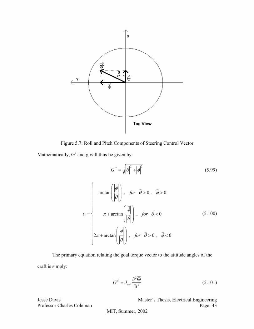
Jesse Davis Master’s Thesis, Electrical Engineering
Professor Charles Coleman Page: 43
MIT, Summer, 2002
Figure 5.7: Roll and Pitch Components of Steering Control Vector
Mathematically, Gc and g will thus be given by:
2 2
CG θ φ= +
r r
(5.99)
arctan , 0 , 0
arctan , 0
2 arctan , 0 , 0
for
g for
for
φθ φ
θ
φπ θ
θ
φπ θ φ
θ
> >
= + <
+ > <
r
r r
r
r
r
r
r
r r
r
(5.100)
The primary equation relating the goal torque vector to the attitude angles of the
craft is simply:
2
2
C
rotG J
t
∂ Θ=
∂
ur
uuur
(5.101)

Jesse Davis Master’s Thesis, Electrical Engineering
Professor Charles Coleman Page: 44
MIT, Summer, 2002
where Jrot is a rotated 2 x 2 inertia matrix given by:
( ) ( )
( ) ( )
( ) ( )
( ) ( )
cos sin cos sin0
0sin cos sin cos
C C C C
o o o oxx
rot C C C Cyy
o o o o
IJ
I
ψ ψ ψ ψ
ψ ψ ψ ψ
− = −
(5.102)
and Θur
is a vector angle given by:
C
C
θ
φ
Θ =
ur
(5.103)
Using the magnitudes of CG
uuur
and Θur
, and assuming that there is a single scalar moment
of inertia, Jscalar, about an axis co-linear with CG
uuur
and Θur
, the Laplace transform of
Equation (5.101) gives:
2
1
Cscalar
J sG
Θ
=
ur
uuur (5.104)
which is the primary equation for which a control law must be determined.
It is apparent from Equation (5.104) that since there are two poles at zero in the
torque-angle system, the system is inherently unstable with a zero degree phase margin.
In order to create a stable system, phase must somewhere by added by a controller. An
ideal controller for this purpose is a lead controller which takes the form:
1
1
c c
c
sLead A
s
α τ
τ
+=
+ (5.105)
A lead controller adds about
1
arcsin1
center
α
α
− Φ =
+ (5.106)
degrees of phase at a frequency of

Jesse Davis Master’s Thesis, Electrical Engineering
Professor Charles Coleman Page: 45
MIT, Summer, 2002
1
centerω
τ α
= (5.107)
The overall gain of the lead controller, A, is adjusted in order to make the cross-over
frequency of the entire system equal to that where the maximum phase of the lead
controller occurs. (A standard upper limit on α is 10. Since a lead controller amplifies
high frequency signal components by a factor of α more than low frequency signal
components, this choice is usually made so as not to overly amplify any high frequency
noise that might corrupt the controller. The maximum phase for an α of 10 is about 55
degrees.)
There is a limit as to how far the bandwidth of the system can be increased,
however. The torque vector is created by the three motors that all have poles associated
with them as well. Taking the Laplace transform of the motor characteristic Equation
(5.7) gives:
( ) ( )2
1/
1
e
m l m la
e m e m
Kb
L I I R I IVs s
K K K K
Ω
=
+ +
+ +
(5.108)
which is a two pole system. (One of the poles of the motor system comes from the
electrical time constant associated with the inductance and resistance, and the other pole
comes from the mechanical time constant of Equation (5.66).) Since every pole subtracts
90 degrees of phase, and there are already two poles at zero from Equation (5.104), the
cross-over frequency of the system must be set at least a decade before the first pole of
Equation (5.108) in order to create a stable system with decent phase margin. Taking all
these factors into consideration, Equations (5.104)-(5.108) can be used to easily
determine the parameters of a lead controller: A, τ, and α.

Jesse Davis Master’s Thesis, Electrical Engineering
Professor Charles Coleman Page: 46
MIT, Summer, 2002
5.3.2.2 Vertical Speed Control
As for the altitude control, a similar simplification will provide much help. Again
using Newton’s Second Law of Motion:
( )3 cos
E
zv
F mt
∂Γ =
∂ (5.109)
where the F is the same as in the motor voltage Equations (5.71)-(5.73). Taking the
Laplace transform of Equation (5.109) and rearranging gives:
( )3cos
E
zv
F ms
Γ= (5.110)
This system only has one pole at the origin, but since F is generated by manipulating
motor voltages, the poles from Equation (5.108) will also still be of concern.
In order to control E
zv , there are now a few different options. Since the pole at the
origin adds only -90 degrees of phase, a simple proportional controller could be used, as
long as the bandwidth is kept well below the first pole of the motor system. In order to
increase the bandwidth as high as possible, however, a lead controller could also be used
with a center frequency in between the two pole frequencies of the motor system. The
second choice is obviously preferable since it will give higher bandwidth leading to faster
control, and a lead controller can be derived in exactly the same way as in the previous
section.
5.3.2.3 Yaw Speed Control
The final controller that needs to be derived is for the yaw speed of the hub. The
yaw speed of the hub is equal to the yaw speed of the hoop minus the speed of the yaw
motor, so in order to control the yaw speed of the hub, the speed of the yaw motor must
be controlled. The equation for the speed of the motor is simply given by Equation

Jesse Davis Master’s Thesis, Electrical Engineering
Professor Charles Coleman Page: 47
MIT, Summer, 2002
(5.108) again! This is just a simple two pole system, and with a lead controller, the cross-
over frequency can now be pushed past the second characteristic motor pole. In fact, with
a lead controller, the gain and cross-over frequency can be made indefinitely high. There
are, of course, limitations to making the gain too high, but these limitations are only
imposed by implementation issues, not by the system itself. For the purposes of
simulation, a lead controller was placed at a frequency about an order of magnitude
greater than the lead of the vertical speed controller.
Jesse Davis Master’s Thesis, Electrical Engineering
Professor Charles Coleman Page: 48
MIT, Summer, 2002
6.0 Simulation
Simulation is used only to verify the theory. Although the theory has been proven
mathematically to be true, it is enlightening to observe the theoretical results by carrying
out numerical simulations. The simulation of the controllers and the simulation of actual
motor voltage commands are performed below. The full state-space model is much more
complicated than the models that were used to derive the controllers, so it is important to
verify that the simplification assumptions were valid. Also, since the dynamic voltages to
the motors that will be used in an actual implementation will be discretized, it is
important to understand the effects this will have on the system.
6.1 Controlled System Step Responses
In order to verify the controllers, simulations were performed using a Matlab ode
solver. Within the Matlab ode file, all of the state equations for the Earth-based frame, as
well as all of the control laws in the Earth-based frame were included. Using the ode
solver, the state equations were stepped forward in time from an initial zero-state starting
point, and by creating time dependent control goals, the operation of the controllers could
be tested.
The lead controlled vertical speed and yaw speed step responses are shown below
in Figures 6.1 and 6.2 respectively. The lead controllers were empirically tuned in order
to get the best responses. As can be seen in Figure 6.1, there is an overshoot in the
vertical speed step response, but the settling time is quite fast so this overshoot is
ignorable. The yaw speed step response has no overshoot, and the reason for this is that
there is 90 degrees more of phase margin in the yaw speed system than in the vertical
speed system. The other important feature of these responses is that they have a zero

Jesse Davis Master’s Thesis, Electrical Engineering
Professor Charles Coleman Page: 49
MIT, Summer, 2002
steady-state error, so that any commanded values will be perfectly met after transients
settle.
Figure 6.1: Vertical Speed Step Responses
Figure 6.2: Yaw Speed Step Responses

Jesse Davis Master’s Thesis, Electrical Engineering
Professor Charles Coleman Page: 50
MIT, Summer, 2002
As for the step responses of the pitch and roll, Matlab was unable to be used to
accurately lead control the steering vector. The reason for this was several discontinuities
encountered when evaluating the derivative of the commanded steering vector to
compute the lead control. The theoretical design of a lead controller for the attitude in
section 5.3.2.1 should be correct, but simulations were unable to be carried out to prove
this fact. Instead, a simple proportional controller was implemented. This approach
worked because a linear damping factor was added to each of the rotational velocities,
and this moved one of the poles at zero slightly off zero. This allowed for a proportional
controller to be used to make a zero-crossing between these first two poles at a much
lower bandwidth than would be expected with the full lead controller. The resulting
proportionally controlled step responses of the pitch and roll are shown below in Figure
6.3:
Figure 6.3: Pitch and Roll Step Responses

Jesse Davis Master’s Thesis, Electrical Engineering
Professor Charles Coleman Page: 51
MIT, Summer, 2002
Overall, the controller design for the vertical speed and yaw speed seems to be
flawless, whereas the controller design for the attitude could use significant
improvement. One important fact that may also be causing problems with the pitch and
roll step responses is the non-linearity of the actual system. It is possible that the
assumptions made in order to simplify the system and derive a simple control law ignore
some fundamental properties of the system that cannot be overlooked. While the
proportional control can be seen to work for a slightly altered system, the controller for
the steering remains an area for future research.
6.2 Time Discretized Dynamic Motor Control
The other simulation that needs to be carried out, besides the step responses of the
controlled system, is of the actual steering torque vector during operation. As was seen in
the system analysis section of the theory, the necessary forces from the motors as they
spin around the hub are sinusoidal in order to properly steer the craft. Since a computer
will eventually be the mechanism that provides the PWM signals to the motors, it would
be difficult to continuously vary the PWM signals as the equations require. Instead, the
computer will most likely have to discretize the PWM variation into a certain number of
segments per rotational period. This will create a discretized sinusoidal torque from each
of the three steering motors, and the effects of this discretization should be simulated in
order to verify that proper steering can still be commanded.
A Matlab file was created that calculated the total torque vector from three
discretized sinusoidal torque vectors with a variable number of discretizations. The inputs
to the file are the number of discretizations per period, the magnitude of the goal torque
vector, GC, and the angle of the goal torque vector, g. The file plots the RxF torque from

Jesse Davis Master’s Thesis, Electrical Engineering
Professor Charles Coleman Page: 52
MIT, Summer, 2002
each of the three motors over hoop rotation angle, the total varying torque vector over
time, and also finds the average torque vector. The complete code for the file can be
found in Appendix A. An example of the torque from each motor over hoop rotation
angle is given in Figure 6.4 below:
-400 -300 -200 -100 0 100 200 300 4003
3.2
3.4
3.6
3.8
4
4.2
4.4
4.6
4.8
5actual discretized torque required by motors
angle, degrees
torque, Nm
motor 1
motor 2
motor 3
Figure 6.4: Example RxF Torques from Each Motor During Steering
It was discovered that both the magnitude and angle of the actual average torque
vector vary significantly with the number of discretizations commanded. The angle
variation was found to be a positive (counter-clockwise) angle offset to the commanded
angle, and the magnitude variation was found to be a less than unity multiple of the
commanded magnitude. These variations are captured in Figures 6.5 and 6.6 below:

Jesse Davis Master’s Thesis, Electrical Engineering
Professor Charles Coleman Page: 53
MIT, Summer, 2002
0 5 10 15 20 25 30 35 40 45 500
10
20
30
40
50
60
70
80
90
discretizations
error angle, degrees
error angle vs. discretizations
Figure 6.5: Error Angle of Actual Average Torque Vector vs. Discretizations
0 5 10 15 20 25 30 35 40 45 500.6
0.65
0.7
0.75
0.8
0.85
0.9
0.95
1
1.05
discretizations
magnitude error factor
magnitude error factor vs. discretizations
Figure 6.6: Magnitude Error Factor vs. Discretizations
Once the discovery of the offset angle and magnitude error were made, the file was
altered to pre-correct for these errors by subtracting the angle offset from the commanded

Jesse Davis Master’s Thesis, Electrical Engineering
Professor Charles Coleman Page: 54
MIT, Summer, 2002
angle, and pre-scaling the commanded magnitude by the inverse of the magnitude error
factor.
The other major variation that occurred with the number of discretizations was the
actual calculated torque variation over time. (The magnitude did not vary significantly in
this regard.) This variation gives a sense of how close the actual torques are to the
average torque over hoop rotation angle. For a commanded 1C
G = and 0g = , Figures
6.7 and 6.8 below give an example torque variation over time and total angular variation
of torques as a function of discretizations:
-1 -0.5 0 0.5 1
-1
-0.5
0
0.5
1
polar plot of torque vector variation resulting from discretizations
calculated torque magnitude, Nm
calculated torque magnitude, Nm
variation
average
G = 1
g = 0
Total Angle of Torque
Variation Over Time
Figure 6.7: Polar Plot of Torque Vector Variation Resulting from Discretizations

Jesse Davis Master’s Thesis, Electrical Engineering
Professor Charles Coleman Page: 55
MIT, Summer, 2002
0 5 10 15 20 25 30 35 40 45 500
20
40
60
80
100
120
discretizations
total angle of torque variation, degrees
total angle of torqe variation over time vs. discretizations
Figure 6.8: Total Angle of Torque Variation Over Time vs. Discretizations
The number of discretizations that were chosen for the actual implementation in
the computer code was based on a need to balance steering precision with computer
processing time. The higher the number of discretizations, the better the precision of the
steering, but also the more processor time required to update the PWM signals. Based on
Figure 6.8 above, 20 discretizations per revolution were chosen.

Jesse Davis Master’s Thesis, Electrical Engineering
Professor Charles Coleman Page: 56
MIT, Summer, 2002
7.0 Design and Construction
Once the theory and simulations were complete, the task turned to building a
working stabilization system. There are two main sections to the system: an on-board,
stabilizing computer, and an off-board user interface and controller. The sub-sections of
the on-board unit are a pitch, roll, yaw sensor, an altimeter, an outer hoop rotation rate
sensor, a receiver for the user’s commands, a central processor, and motor driver
circuitry. The sub-sections of the off-board unit are a user interface, a command
serializer, and a transmitter for sending commands to the craft. The primary goal behind
the design of the system was modularity. This methodology simplifies the design,
construction, and debugging, and for a complex system, breaking the problem into parts
aids greatly. The remainder of this section will describe in detail the actual design and
construction of both the hardware and software needed to create a working system.
Unforeseen problems that arose during this process will be discussed, and solutions that
were implemented will be described.
7.1 User Interface and Off-Board Controller
The main sections of the off-board unit are the user interface, a command
serializer, and a transmitter. The user interface is implemented in a simple and widely
used method of using a two-axis potentiometer as a joystick. A two-axis potentiometer
joystick is a single unit in which there are two potentiometers mounted in such a way that
a single stick moved in orthogonal directions will create varying resistances in two
orthogonal potentiometers. Voltages from the potentiometers center-tap can then be
interpreted as user input commands. The complete block diagram of the off-board system
is shown in Figure 7.1 below:
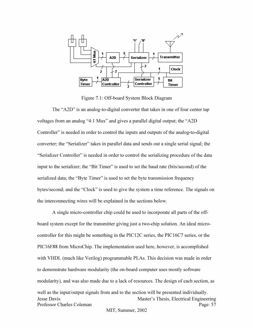
Jesse Davis Master’s Thesis, Electrical Engineering
Professor Charles Coleman Page: 57
MIT, Summer, 2002
Figure 7.1: Off-board System Block Diagram
The “A2D” is an analog-to-digital converter that takes in one of four center tap
voltages from an analog “4:1 Mux” and gives a parallel digital output; the “A2D
Controller” is needed in order to control the inputs and outputs of the analog-to-digital
converter; the “Serializer” takes in parallel data and sends out a single serial signal; the
“Serializer Controller” is needed in order to control the serializing procedure of the data
input to the serializer; the “Bit Timer” is used to set the baud rate (bits/second) of the
serialized data; the “Byte Timer” is used to set the byte transmission frequency
bytes/second; and the “Clock” is used to give the system a time reference. The signals on
the interconnecting wires will be explained in the sections below.
A single micro-controller chip could be used to incorporate all parts of the off-
board system except for the transmitter giving just a two-chip solution. An ideal micro-
controller for this might be something in the PIC12C series, the PIC16C7 series, or the
PIC16F88 from MicroChip. The implementation used here, however, is accomplished
with VHDL (much like Verilog) programmable PLAs. This decision was made in order
to demonstrate hardware modularity (the on-board computer uses mostly software
modularity), and was also made due to a lack of resources. The design of each section, as
well as the input/output signals from and to the section will be presented individually.

Jesse Davis Master’s Thesis, Electrical Engineering
Professor Charles Coleman Page: 58
MIT, Summer, 2002
7.1.1 Multiplexer and Analog-to-Digital Converter
Inputs: center-tap from each of four potentiometers on the two joysticks
data_select 0,1: two bit data selector from A2D Controller
nread: active-low conversion enable signal from A2D Controller
Outputs: nconv_done: active-low conversion complete signal to A2D Controller
data_in 1-5: five parallel digital lines to Serializer
The only two parts of Figure 7.1 that were combined into a single chip solution
were the multiplexer and analog-to-digital converter. The chip that was used for this was
the AD7824 which is a four-channel, 8-bit ADC. The fastest cycle time for switching
input channels and converting to a stable output is 2.5us corresponding to 400kHz. This
frequency turns out not to be the limiting factor to define the number of bytes per second
that the controller can send at top speed, but it is an important upper limit to note for the
proper use of this ADC.
The inputs to the four analog channels of the ADC are the center-taps from the
joystick potentiometers. The channel selection and active-low conversion enable are
controlled by the A2D Controller. As will be described in a subsequent section, the A2D
Controller waits for the Serializer to finish sending the data from the ADC before
switching input channels and requesting another conversion. The outputs of the ADC are
the parallel digital converted data which is sent directly to the Serializer for transmission,
and the conversion complete signal sent to the A2D Controller. The reason all eight bits
are not sent to the Serializer is in order to conserve the number of bits per byte of
transmission, and also because the full resolution should not be necessary to still have

Jesse Davis Master’s Thesis, Electrical Engineering
Professor Charles Coleman Page: 59
MIT, Summer, 2002
very precise control of the craft. The active-low conversion complete signal is sent to the
A2D Controller which then alerts the Serializer Controller that new data is ready to be
sent by the Serializer.
7.1.2 Byte Timer
Inputs: no signal inputs from any other section
Outputs: tx_trigger: active-high data transmission trigger to A2D Controller
The Byte Timer has the purpose of setting the frequency of transmission of bytes
from the off-board unit. The choice of byte frequency can be made rather arbitrarily, with
the main three restrictions being that the command updates should be fast enough to
control the craft precisely, slow enough that the on-board computer doesn’t get
overloaded with data, and slow enough that bytes don’t overlap each other. Since the
baud rate was chosen to be about 2400 (for reasons that will be explained shortly), and
there are a total of 10 bits to a standard serial byte transmission, the maximum frequency
of non-overlapping bytes per second is 240Hz. In order not to push this maximum, the
choice was made to update each of the four command channels at a rate approximately
equal to the inherent update rates of the Pitch, Roll, Yaw Sensor and Altimeter.
The implementation of the Byte Timer was accomplished with a 555 timer setup
in an astable oscillation mode as in Figure 7.2 below:
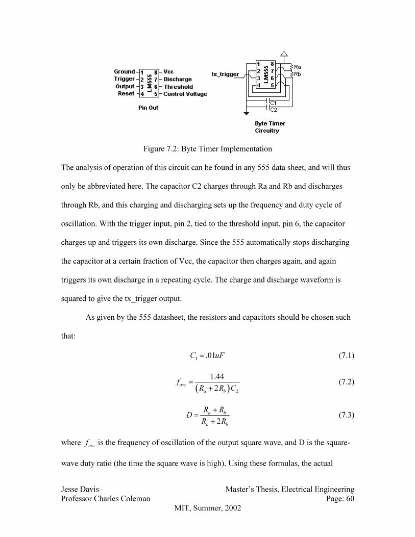
Jesse Davis Master’s Thesis, Electrical Engineering
Professor Charles Coleman Page: 60
MIT, Summer, 2002
Figure 7.2: Byte Timer Implementation
The analysis of operation of this circuit can be found in any 555 data sheet, and will thus
only be abbreviated here. The capacitor C2 charges through Ra and Rb and discharges
through Rb, and this charging and discharging sets up the frequency and duty cycle of
oscillation. With the trigger input, pin 2, tied to the threshold input, pin 6, the capacitor
charges up and triggers its own discharge. Since the 555 automatically stops discharging
the capacitor at a certain fraction of Vcc, the capacitor then charges again, and again
triggers its own discharge in a repeating cycle. The charge and discharge waveform is
squared to give the tx_trigger output.
As given by the 555 datasheet, the resistors and capacitors should be chosen such
that:
1
.01C uF= (7.1)
( ) 2
1.44
2osc
a b
fR R C
=
+
(7.2)
2
a b
a b
R RD
R R
+
=
+
(7.3)
where oscf is the frequency of oscillation of the output square wave, and D is the square-
wave duty ratio (the time the square wave is high). Using these formulas, the actual

Jesse Davis Master’s Thesis, Electrical Engineering
Professor Charles Coleman Page: 61
MIT, Summer, 2002
values that were chosen are: C1 = .01uF, C2 = .1uF, Ra = 39kΩ, and Rb = 39kΩ. In
testing, the oscillation frequency was about 145Hz. (Note: the duty ratio of the signal
doesn’t matter since it is only the frequency of low to high transitions that affects the rest
of the system.)
7.1.3 A2D Controller
Inputs: clk: system clock
nconv_done: active-low conversion complete signal from ADC
txdone: active-high data transmission complete signal from Serializer Controller
tx_trigger: active-high data transmission trigger from Byte Timer
Outputs: data_select 0,1: two bit data selector to ADC and Serializer
nread: active-low conversion enable signal to ADC
data_ready: active-high data ready signal to Serializer Controller
The A2D Controller controls the selection and conversion of the analog joystick
data via the ADC. The logic behind the controller is very direct. When triggered by the
rising edge of tx_trigger from the Byte Timer, the controller initiates a conversion of one
of the four analog inputs by issuing a two bit data_select signal, to choose the analog
input, and pulling low the active-low ADC read trigger, nread. The A2D Controller then
goes into a wait state until the analog-to-digital conversion is complete, as signaled by the
nconv_done line being pulled low by the ADC. At the end of a conversion, the A2D
Controller alerts the Serializer Controller that new digital data is on the bus between the
ADC and Serializer. Again the A2D Controller goes into a wait state until it is signaled
by the Serializer Controller, which eventually pulls txdone high, signifying that the

Jesse Davis Master’s Thesis, Electrical Engineering
Professor Charles Coleman Page: 62
MIT, Summer, 2002
transmission of the data is complete. The A2D Controller then updates the data_select
bus to select the next analog input, and resets to its initial state to wait for the trigger from
the Byte Timer again.
The controller is implemented as a finite state machine in a VHDL programmed
PLA. As was already mentioned, instead of using a single micro-controller and
programming in a more powerful language, such as C, several PLAs were used in order
to demonstrate hardware modularity. Also, finite state machines are particularly easy to
write in VHDL, and for all three programmed parts, the A2D Controller, the Serializer,
and the Serializer Controller, finite state machines were straightforward architectures.
The complete VHDL code for these three off-board components is included in Appendix
B.
7.1.4 Serializer
Inputs: clk: system clock
txbit: bit transmit signal from Serializer Controller
txdone: active-high data transmission complete signal from Serializer Controller
data_in 0-9: ten parallel digital lines from ADC, A2D Controller, and three
switches
Outputs: data_out: serialized data output to Transmitter
The Serializer takes ten parallel digital inputs and time multiplexes them into a
single serial output. The Serializer is controlled by two signals from the Serializer
Controller, txbit and txdone. Most of the time, the Serializer is in a wait state. The rising
edge of the bit transmit command, txbit, triggers the Serializer to read an internal register
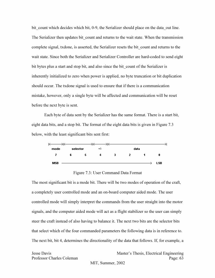
Jesse Davis Master’s Thesis, Electrical Engineering
Professor Charles Coleman Page: 63
MIT, Summer, 2002
bit_count which decides which bit, 0-9, the Serializer should place on the data_out line.
The Serializer then updates bit_count and returns to the wait state. When the transmission
complete signal, txdone, is asserted, the Serializer resets the bit_count and returns to the
wait state. Since both the Serializer and Serializer Controller are hard-coded to send eight
bit bytes plus a start and stop bit, and also since the bit_count of the Serializer is
inherently initialized to zero when power is applied, no byte truncation or bit duplication
should occur. The txdone signal is used to ensure that if there is a communication
mistake, however, only a single byte will be affected and communication will be reset
before the next byte is sent.
Each byte of data sent by the Serializer has the same format. There is a start bit,
eight data bits, and a stop bit. The format of the eight data bits is given in Figure 7.3
below, with the least significant bits sent first:
Figure 7.3: User Command Data Format
The most significant bit is a mode bit. There will be two modes of operation of the craft,
a completely user controlled mode and an on-board computer aided mode. The user
controlled mode will simply interpret the commands from the user straight into the motor
signals, and the computer aided mode will act as a flight stabilizer so the user can simply
steer the craft instead of also having to balance it. The next two bits are the selector bits
that select which of the four commanded parameters the following data is in reference to.
The next bit, bit 4, determines the directionality of the data that follows. If, for example, a

Jesse Davis Master’s Thesis, Electrical Engineering
Professor Charles Coleman Page: 64
MIT, Summer, 2002
30 degree pitch is commanded, this bit will decide whether the pitch is forward or
backward. For the thrust parameter in the user controlled mode, this bit will be an
additional data bit because there will not be the possibility of negative thrust. Finally, the
last four bits are the actual data bits. Four bits, including the positive or negative bit, will
give 31 total possible commands per parameter. (The thrust will have 32 commands.)
The Serializer was implemented on a PLA programmed in VHDL with a finite
state machine architecture. The interesting aspect of the Serializer implementation was
the method of catching the rising edge of the bit transmit signal, txbit. Since the
transmission complete signal, txdone, is independent of txbit, txbit could not be used as
the Serializer’s clock input because the txdone signal would never be read. Thus the
system clock had to be used as the Serializer’s clock. If txbit lasted for more than one
clock cycle, however, the Serializer might send a subsequent bit far sooner than expected,
thus garbling the transmission. In order to trigger on only the rising edge of txbit, a flag
was used in the VHDL code to indicate whether or not txbit had gone low since the last
time it had been high. If txbit was read high but had not gone low since the last time it
was read high, the same high txbit signal must be being read twice. If txbit was read high
and had been read low since the last time it was read high, txbit must have just gone high,
and the rising edge was caught. A code snippet of this logic is immediately below. For
the full VHDL code see Appendix B.
... if rising_edge(clk) then if (txdone = '1') then data_out <= '0'; bit_count <= "0000"; flag <= '0'; elsif (txbit = '0') then flag <= '0';

Jesse Davis Master’s Thesis, Electrical Engineering
Professor Charles Coleman Page: 65
MIT, Summer, 2002
elsif ((txbit = '1') and (flag = '0')) then flag <= '1'; case bit_count is
...
end if
...
7.1.5 Serializer Controller
Inputs: clk: system clock
data_ready: active-high data ready signal from A2D Controller
per_counter 0-3: four-bit baud period counter from Bit Timer
Outputs: en_nres: active-high counter enable, active-low counter reset to Bit Timer
txbit: bit transmit signal to Serializer
txdone: active-high data transmission complete signal to A2D Controller and
Serializer
The Serializer Controller controls the data transmission of the off-board unit. It
enables and resets the Bit Timer which sets the baud rate, it triggers the Serializer to send
bits at the correct times, and it signals the A2D Controller to update the data after a
transmission is complete. There are several stages to the operation of the Serializer
Controller. After the Bit Timer is reset and enabled, the Serializer Controller waits until
the time required between each bit is counted by the Bit Timer. At the end of this time,
the Serializer Controller triggers the Serializer to send a bit, and restarts the Bit Timer.
After ten bits have been sent, the Serializer Controller alerts both the Serializer and the
A2D Controller that the transmission is complete. This transmission complete signal
resets the Serializer’s bit_count so that the next bit to be sent will be the data 0 bit, and it

Jesse Davis Master’s Thesis, Electrical Engineering
Professor Charles Coleman Page: 66
MIT, Summer, 2002
also tells the A2D Controller to trigger the ADC for new data when the Byte Timer
triggers it.
The Serializer Controller was implemented as a finite state machine in VHDL.
The full code is given in Appendix B.
7.1.6 Bit Timer
Inputs: en_nres: active-high counter enable, active-low counter reset from Serializer
Controller
clk: system clock
Outputs: per_counter 0-3: four-bit baud period counter to Serializer Controller
The only purpose of the Bit Timer is to act as a binary counter that can be reset at
any time and enabled and disabled to count. This is precisely what the LS163 IC can do,
and additionally, the LS163 can be daisy-chained to provide slower and slower counting.
Since the speed of the system clock was 1.8432MHz, and the baud rate required was
2400, the clock had to be divided by 768 by the Bit Counter. This required three LS163’s
where bits 8 and 9 of the total counter where used as the baud period timer by the Serial
Controller. (768=512+256.) The complete implementation of the Bit Timer is shown in
Figure 7.3 below:
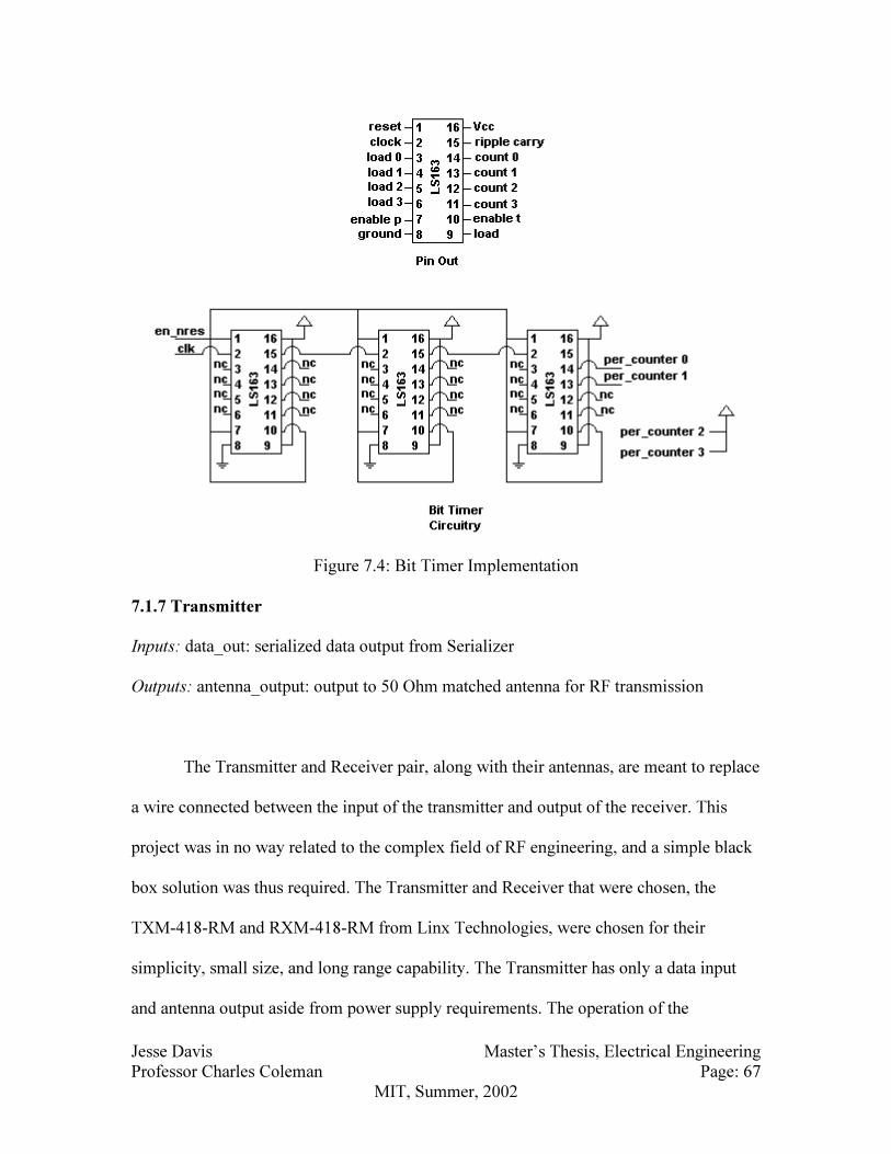
Jesse Davis Master’s Thesis, Electrical Engineering
Professor Charles Coleman Page: 67
MIT, Summer, 2002
Figure 7.4: Bit Timer Implementation
7.1.7 Transmitter
Inputs: data_out: serialized data output from Serializer
Outputs: antenna_output: output to 50 Ohm matched antenna for RF transmission
The Transmitter and Receiver pair, along with their antennas, are meant to replace
a wire connected between the input of the transmitter and output of the receiver. This
project was in no way related to the complex field of RF engineering, and a simple black
box solution was thus required. The Transmitter and Receiver that were chosen, the
TXM-418-RM and RXM-418-RM from Linx Technologies, were chosen for their
simplicity, small size, and long range capability. The Transmitter has only a data input
and antenna output aside from power supply requirements. The operation of the
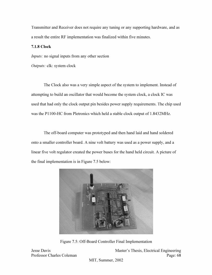
Jesse Davis Master’s Thesis, Electrical Engineering
Professor Charles Coleman Page: 68
MIT, Summer, 2002
Transmitter and Receiver does not require any tuning or any supporting hardware, and as
a result the entire RF implementation was finalized within five minutes.
7.1.8 Clock
Inputs: no signal inputs from any other section
Outputs: clk: system clock
The Clock also was a very simple aspect of the system to implement. Instead of
attempting to build an oscillator that would become the system clock, a clock IC was
used that had only the clock output pin besides power supply requirements. The chip used
was the P1100-HC from Pletronics which held a stable clock output of 1.8432MHz.
The off-board computer was prototyped and then hand laid and hand soldered
onto a smaller controller board. A nine volt battery was used as a power supply, and a
linear five volt regulator created the power buses for the hand held circuit. A picture of
the final implementation is in Figure 7.5 below:
Figure 7.5: Off-Board Controller Final Implementation

Jesse Davis Master’s Thesis, Electrical Engineering
Professor Charles Coleman Page: 69
MIT, Summer, 2002
7.2 On-Board Computer
The on-board computer is also broken into several parts. The architecture of the
on-board computer uses a master controller to collect data from several sensors, as well
as command data from the off-board controller, and process these data into PWM signals
sent to four motor drivers to steer the craft. This architecture is captured by Figure 7.6
below:
Figure 7.6: System Block Diagram
As discussed in the control section of the theory, an Altimeter, Pitch, Roll, Yaw Sensor,
and an Outer Hoop Rotation Rate Sensor are the minimum necessary sensors needed to
fly the craft. The CPU Data Interface is required because of some very specific issues
with the communication protocols available on the CPU. Since each of these sensors
needs to be interfaced in an entirely different manner, the CPU code demonstrates a wide
variety of the functionality of the particular CPU chosen.
The Altimeter and Pitch, Roll, Yaw Sensor are both polled by the CPU for data,
while the Outer Hoop Rotation Rate Sensor and Receiver both continuously transmit data
to the CPU. The Altimeter and Outer Hoop Rotation Rate Sensor data transmissions
interrupt the processor when they are received since the sensors are inherently
asynchronous as will be described. The Pitch, Roll, Yaw Sensor and Receiver data inputs

Jesse Davis Master’s Thesis, Electrical Engineering
Professor Charles Coleman Page: 70
MIT, Summer, 2002
are serial and are buffered in software by background processes. The formatting of each
set of data is also very different. The Outer Hoop Rotation Rate Sensor signal is a square
wave with a period equal to the period of rotation of the hoop around the hub; the
Altimeter signal is a pulse with a width proportional to the altitude of the craft; the Pitch,
Roll, Yaw Sensor has a manufacturer specified seven byte response format; and the
command data from the user that comes in from the Receiver has a custom format given
in Figure 7.3 and explained in the Serializer section of the off-board controller above.
Each section of the on-board computer is explained in detail below. Since most of
the components were purchased and not designed and built as part of the project,
descriptions of the communications protocols and basic operating characteristics about
the specific devices are all that will be provided. For more detailed information, see the
manufacturers’ data sheets. As for the CPU section, all of the work necessary was done in
software, so the general structure of this code will be given, and the full text of the code
will be provided in Appendix C.
7.2.1 Outer Hoop Rotation Rate Sensor
Inputs: no signal inputs from any other section
Outputs: rotation_clock: square wave signal with period matched to hoop rotation around
hub to CPU
The primary purpose of the Outer Hoop Rotation Rate Sensor is to determine how
fast the hoop is spinning with respect to the hub. The sensor also provides a reference for
the angle between the front of the craft (the front of the hub). Both of these data are
needed in order to properly control the steering voltage signals to the motors, and thus in

Jesse Davis Master’s Thesis, Electrical Engineering
Professor Charles Coleman Page: 71
MIT, Summer, 2002
order to properly control the craft. (One other piece of information that may be given by
this sensor is the actual angle between the front of the craft and the location of the
motors, and not just a reference for it. Depending on the particular parts used in the
implementation, this information either will or will not be accurately available.)
In order to determine the rate of rotation in a simple manner, the wrap around on
the center tap of a potentiometer will be detected. With one end of the potentiometer
mounted on the hub, and one end of the potentiometer mounted on the hoop, the voltage
on the center tap of the potentiometer should ideally be a saw-tooth wave with the same
frequency as the rotation frequency of the hoop. In the implementation given here, this
saw-tooth wave is squared to give a square wave clock with clean transitions that can
easily be detected by the CPU. The total circuit is provided in Figure 7.7 below:
Figure 7.7: Outer Hoop Rotation Rate Sensor Implementation
Since the wrap around is linked to the physical spinning of the hoop, the angular
placement of the potentiometer can be made such that the wrap around corresponds to a
certain orientation between hoop and hub. If a full turn potentiometer is used, instead of
the more standard partial turn potentiometers, the actual location of the hoop in relation
to the hub can be determined at any time. In the current implementation, a partial turn
potentiometer was used so that the only useful information given by the sensor is an
angular rate and angular reference and not any angles themselves. It is hoped that, other

Jesse Davis Master’s Thesis, Electrical Engineering
Professor Charles Coleman Page: 72
MIT, Summer, 2002
than at start-up, the rotation rate of the hoop will vary only slowly in relation to its own
speed so that the angular data can be created from the angular rate data and angular
reference.
7.2.2 Altimeter
Inputs: alt_query: negative transition query signal from CPU Data Interface
Outputs: echo: output relating to altitude of craft to CPU
The altimeter that was chosen is an ultrasonic range finder that is accurate
between three centimeters and three meters. The range finder works by sending out a
burst of ultrasonic tones and waiting for the echo to return. The length of time of the echo
then determines how far away the nearest object is since the speed of sound in air is fairly
constant under normal conditions. The specific ranger that was used, the Devantech
SRF04, requires a falling transition trigger, alt_query, and then responds with a signal,
echo, that has a high time proportional to the distance of the nearest object. The high time
of the echo signal is specified at 36 milliseconds when no ultrasonic echo is recorded by
the ranger. There is also a mandatory specified 10 millisecond delay between the end of
the echo signal and another falling transition of alt_query. This corresponds to a
maximum querying rate of 21.74Hz, so in order not to push the limit, the altimeter was
queried at 20Hz. Data taken on the ranger at four centimeter increments from four
centimeters to over three meters is shown in Figure 7.8 below:
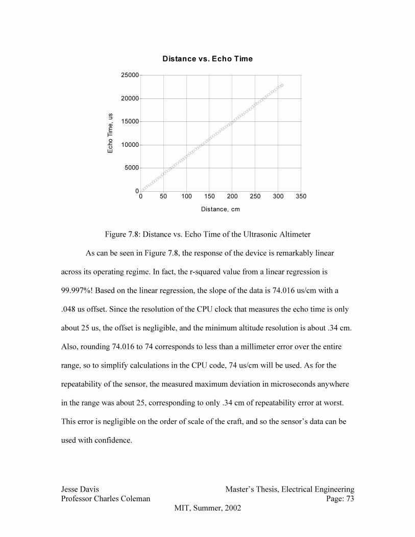
Jesse Davis Master’s Thesis, Electrical Engineering
Professor Charles Coleman Page: 73
MIT, Summer, 2002
Distance vs. Echo Time
0
5000
10000
15000
20000
25000
0 50 100 150 200 250 300 350
Echo T
ime
, u
s
Distance, cm
Figure 7.8: Distance vs. Echo Time of the Ultrasonic Altimeter
As can be seen in Figure 7.8, the response of the device is remarkably linear
across its operating regime. In fact, the r-squared value from a linear regression is
99.997%! Based on the linear regression, the slope of the data is 74.016 us/cm with a
.048 us offset. Since the resolution of the CPU clock that measures the echo time is only
about 25 us, the offset is negligible, and the minimum altitude resolution is about .34 cm.
Also, rounding 74.016 to 74 corresponds to less than a millimeter error over the entire
range, so to simplify calculations in the CPU code, 74 us/cm will be used. As for the
repeatability of the sensor, the measured maximum deviation in microseconds anywhere
in the range was about 25, corresponding to only .34 cm of repeatability error at worst.
This error is negligible on the order of scale of the craft, and so the sensor’s data can be
used with confidence.
Jesse Davis Master’s Thesis, Electrical Engineering
Professor Charles Coleman Page: 74
MIT, Summer, 2002
7.2.3 Pitch, Roll, Yaw Sensor
Inputs: pry_query: formatted one byte serial request from CPU Data Interface
Outputs: pry_data: formatted seven byte serial response to CPU Data Interface
The Pitch, Roll, Yaw Sensor used, a MicroStrain 3DM-DH, uses several
orthogonal accelerometers and magnetometers to determine the attitude of the craft. The
detailed inner workings of the sensor are complicated and unnecessary to present here.
The manufacturer supplied specifications are an accuracy of ± .7 degrees in pitch and
roll, and ± 1.5 degrees in yaw each with resolutions of less than .1 degrees. The usable
range of the pitch and yaw is ± 180 degrees, and the usable range of the roll is ± 70
degrees. The pitch, roll, and yaw data is updated at a maximum rate of about 30Hz, and is
communicated using an RS-232 serial protocol at 9600 baud.
The greatest benefit of the sensor is that it requires no initialization routine which
would cause a startup delay and also complicate the CPU code. The one setup that could
be done is to tare all the pitch, roll, and yaw values, but these tares can be handled in the
CPU so that the only request from the CPU will be for pitch, roll, and yaw data. Also, the
Pitch, Roll, Yaw Sensor requires the same voltage range as does the CPU, so only one
power supply needs to be used. With the ease of integration and communication, the
precision and accuracy of the sensor, as well as the physical size of the sensor package,
the MicroStrain sensor is ideal for the craft. (A new version of the MicroStrain sensor has
just been released which also includes angular rate gyroscopes. This new sensor is
unaffected by the movement of the craft itself, and will work in any dynamic as well as
static environment. The sensor used in this project is meant only for a static environment,

Jesse Davis Master’s Thesis, Electrical Engineering
Professor Charles Coleman Page: 75
MIT, Summer, 2002
but the accelerations experienced by the craft should be small compared to the effects of
gravity, so the sensor deviation will be minimal. For a future design, the new sensor, the
3DM-G should be used.)
7.2.4 Receiver
Inputs: antenna_input: input from 50 Ohm matched antenna for RF reception
Outputs: user_data: formatted one byte serial data to CPU Data Interface
detect: analog data detect signal to CPU
The receiver’s main function is to receive digital serial data from the transmitter
on the off-board controller. Since the receiver will always be picking up noise from the
environment, even if the transmitter is turned off, one additional requirement of the
receiver is to also have an output that alerts the CPU to the presence or absence of a
strong carrier signal from the transmitter. This detect output is essentially a data
validation output, and if it is not active, the data that is being sent out of the receiver must
be spurious.
The receiver used has exactly and only these two outputs. As mentioned in the
Transmitter section of the off-board controller above, RF engineering was not a major
part of the design work of this project, and a black box solution was sought. The TXM-
418-RM and RXM-418-RM from Linx Technologies were chosen as the
Transmitter/Receiver pair, and they were both matched with an ANT-418-CW-RH
antenna giving a manufacturer specified line-of-sight range of over 500 feet. The main
drawback to the communications link is that the Linx components are specified to only
handle data rates up to 10K baud. In testing, the maximum safe error-free standard baud

Jesse Davis Master’s Thesis, Electrical Engineering
Professor Charles Coleman Page: 76
MIT, Summer, 2002
rate was found to be 2400. As was mentioned in the Byte Timer section of the off-board
controller above, this limits the maximum byte rate to 240Hz. If a higher speed system
were desired, with a higher user command update rate, a new Transmitter/Receiver pair
would need to be found.
The only unexpected issue with the Receiver hardware implementation was with
the detect output. The detect output is not a standard digital output, and its voltage varies
by only a very slight amount between on and off states. As a result, a conversion of the
detect output into a digital signal was required. Since the CPU has eight analog-to-digital
converter inputs, however, no special off-CPU hardware was needed, and the conversion
could be handled in software on the CPU. The proper loading of the detect pin was still
required, however, and it was discovered that a 1MΩ resistor was required from the
detect pin to ground in order to significantly differentiate the on and off outputs.
7.2.5 CPU Data Interface
Inputs: pry_data: formatted seven byte serial response from Pitch, Roll, Yaw Sensor
user_data: formatted one byte serial data from Receiver
alt_query_clock: 4x speed PWM altimeter query signal from CPU
pry_query_fromCPU: one byte serial request to Pitch, Roll, Yaw Sensor in the
serial protocol of the CPU to the CPU Data Interface
Outputs: alt_query: PWM altimeter query signal to Altimeter
pry_query: one byte serial request to Pitch, Roll, Yaw Sensor
pry_data_toCPU: formatted seven byte serial response from Pitch, Roll, Yaw
Sensor altered to the serial protocol of the CPU to the CPU

Jesse Davis Master’s Thesis, Electrical Engineering
Professor Charles Coleman Page: 77
MIT, Summer, 2002
user_data_toCPU: formatted one byte serial data from the Receiver altered to the
serial protocol of the CPU to the CPU
The CPU Data Interface was not an original component of the system design, and
was discovered to be necessary after extensive testing of the CPU. The CPU has two
dedicated programmable hardware serial ports, but the hardware interface for these ports
requires more hardware design work to be done than seems reasonably necessary for this
project. The other serial possibilities are 14 general purpose programmable I/O pins on
the CPU, so these were chosen to be used instead. The interesting aspect of the serial
communication from these pins, however, is that the pins can only be driven between 0
and 5 volts opposed to the standard -12 and 12 volts, and also the voltages are inverted
from standard RS-232 protocol. In other words, instead of 5 volts corresponding to 12
volts and 0 volts corresponding to -12 volts, 5 volts corresponds to -12 volts and 0 volts
corresponds to 12 volts.
The three serial inputs of the CPU Data Interface are thus simply inverted to
become the correct serial outputs. Since the only bi-directional serial communication
occurred with the Pitch, Roll, Yaw Sensor, and it was discovered that this sensor could
detect serial communications between 0 and 5 volt levels, only an inverter is required,
and no more hardware intensive level changer. The inverter must sustain ± 12 volt inputs,
however, but this is not a difficult constraint to meet. All this leads to the fact that the
digital signal processing that the CPU Data Interface provides gives
_ _ _pry query pry query fromCPU= and _ _ _pry data toCPU pry data= .
Jesse Davis Master’s Thesis, Electrical Engineering
Professor Charles Coleman Page: 78
MIT, Summer, 2002
Since the user command data coming from the receiver is specifically formatted
in the off-board controller, there is a choice as to whether or not to put the data through
an inverter on the on-board computer or to invert it before transmission. Since the CPU
would require that a high voltage level be held across the RF channel unless data was
being received, it was decided to invert the data on the on-board computer since holding a
non-zero level can be difficult over an RF link. Thus another conversion that the CPU
Data Interface provides is _ _ _user data toCPU user data= .
The other interfacing that the CPU Data Interface provides is for the altimeter
querying. As specified in the Altimeter section of the off-board controller above, the
querying rate of the Altimeter is 20Hz. This specification is precisely met by a PWM
signal from the CPU. In order to use the built-in software serial communication routines
for the other data I/O lines, however, the minimum frequency PWM signal from the CPU
is about 125Hz. In order to provide a proper trigger for the Altimeter, a frequency
reduction is thus required. It was chosen to program the CPU to give a 160Hz
alt_query_clock signal that is frequency divided 8 times by a three bit counter on the
CPU Data Interface. The CPU Data Interface uses the alt_query_clock signal as a clock
input that cycles a finite state machine through eight possible states. In only one of these
states, the altimeter query signal, alt_query, is brought high, and the negative transition of
this signal triggers the Altimeter to take a measurement. The high time requirement of the
alt_query signal specified by the Altimeter manufacturer of 10 microseconds is also
easily met by this 6.25 millisecond high time trigger.
The CPU Data Interface is implemented on a VHDL programmed PLA. The three
necessary inverters are made as non-clocked, non-latched inverters so that the
Jesse Davis Master’s Thesis, Electrical Engineering
Professor Charles Coleman Page: 79
MIT, Summer, 2002
communication between the CPU and Altimeter would be completely independent of the
other CPU communication. The complete VHDL code for the CPU Data Interface is
provided in Appendix B.
7.2.6 Motor Drivers 1-3 and Yaw Motor Driver
Inputs: PWM 1-3, Yaw: PWM signals for motors from CPU
Outputs: Power amplified PWM signals to motors
The final sections of the on-board computer to be described besides the actual
CPU are the Motor Drivers for the three steering motors and the one yaw motor. The
main requirement on the Motor Drivers is that they be able to create sharp transitions for
a high power output PWM signal. The PWM frequency required will be specified by the
types of motors to be used in the construction of the craft. Since the actual craft
construction is not a part of this project, the specific motors for implementation were not
chosen, so a definite PWM frequency could not be chosen. In order to supply a relatively
constant voltage to a motor, a PWM frequency should be at least 10 times higher than the
inherent electrical time constant frequency. For most standard miniature DC motors, a
PWM frequency of 40KHz is more than ample, and so this is the PWM frequency that
was chosen. The switching time of the PWM signal should be at least about 100 times
faster than the PWM period, so the Motor Drivers need to be able to switch the full
system voltage, Vmax, in 250 nanoseconds.
As for the current sourcing requirement of the Motor Drivers, some thrust theory
will need to be done in order to determine power requirements for the craft. From
Jesse Davis Master’s Thesis, Electrical Engineering
Professor Charles Coleman Page: 80
MIT, Summer, 2002
Bernoulli’s Law, pressure is dependent on velocity of a fluid, and it can be determined
that:
21
2o inP P vρ= + (7.4)
where Po is the ambient non-moving air pressure well above the propeller, P is the air
pressure just above the propeller, ρ is the air density, and vin is the downward velocity of
the air just above the propeller. The pressure just below the propeller will be P P+ ∆ and
will be moving with a velocity of vin, and the pressure well below the propeller will again
be Po and will be moving with a velocity vout. Using these observations gives the
following equality:
2 2 2 21 1 1 1
2 2 2 2o out in out inP v P v v P P vρ ρ ρ ρ+ = + + = + ∆ + (7.5)
and solving for P∆ yields:
21
2out
P vρ∆ = (7.6)
In order to create this pressure differential, a thrust, Cf , is required by the
propeller:
2 2 21
2
C
prop prop outf R P R vπ ρπ= ∆ = (7.7)
This thrust can also be written in terms of a mass flux, Φ , as:
2C
out prop in outf v R v vρπ= Φ = (7.8)
Equating Equations (7.7) and (7.8) gives:
2out inv v= (7.9)
Jesse Davis Master’s Thesis, Electrical Engineering
Professor Charles Coleman Page: 81
MIT, Summer, 2002
In order produce this required thrust, the propeller must be supplied with some
amount of power. This required power, Ppow, is:
2 2 2 2 31 1 1
2 2 4pow out prop in out prop out
P v R v v R vρπ ρπ= Φ = = (7.10)
Rearranging Equation (7.7) in order to find the required vout for a given thrust gives:
2
2C
out
prop
fv
Rρπ= (7.11)
and substituting Equation (7.11) into Equation (7.10), the power required for a given
thrust is:
3
22
C
pow
prop
fP
Rρπ= (7.12)
If the maximum voltage in the system is Vmax, the motors have an efficiency of η for
converting electrical power into mechanical power, and the maximum thrust is max
Cf , the
maximum current, Imax, required by the Motor Drivers will be:
3
max
max 2
max
1
2
C
prop
fI
V Rη ρπ= (7.13)
If a 4 inch propeller blade is used, the maximum thrust is limited to twice the
weight of the craft, the mass of the craft is 700 grams, the efficiency of the motors is
50%, and the maximum system voltage is 20 volts, the maximum necessary continuous
current required from the Motor Drivers is 6 amps. There are several possible power
transistors that will supply this necessary power. Three possible suppliers of such
transistors are Mospec Semiconductor, Toshiba Semiconductor, and Fairchild
Semiconductor. The largest problem with finding these transistors will be matching both

Jesse Davis Master’s Thesis, Electrical Engineering
Professor Charles Coleman Page: 82
MIT, Summer, 2002
the high current requirement and fast switching requirement, but transistors close to the
specifications certainly exist. Two possible transistors for this purpose are the BU326
from Mospec or the KSC3552 from Fairchild.
One significant problem with these high power output transistors is that they have
extremely low beta values, so the base current may have to be up to one-tenth of the
collector current. This means that for a 6 amp output, the signal driving the transistor has
to source 600 milliamps! This high driving current requires that a pre-amplifier also be
used between the power amplifying transistors and the CPU. This pre-amplifier, besides
supplying the necessary driving current for the output stage transistors, needs to be high-
speed and also needs to convert the 0 to 5 volt digital signal from the CPU into a 0 to
Vmax volt signal. One possible amplifier that will do this is the LM4765 from National
Semiconductor.
Since the motors that will be used on the actual craft have not been chosen, the
components used in the Motor Drivers remain unspecified here. A general topology of
the Motor Drivers might be as shown in Figure 7.9 below, however:
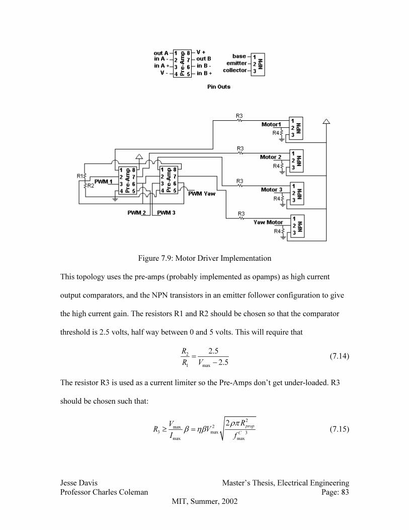
Jesse Davis Master’s Thesis, Electrical Engineering
Professor Charles Coleman Page: 83
MIT, Summer, 2002
Figure 7.9: Motor Driver Implementation
This topology uses the pre-amps (probably implemented as opamps) as high current
output comparators, and the NPN transistors in an emitter follower configuration to give
the high current gain. The resistors R1 and R2 should be chosen so that the comparator
threshold is 2.5 volts, half way between 0 and 5 volts. This will require that
2
1 max
2.5
2.5
R
R V=
−
(7.14)
The resistor R3 is used as a current limiter so the Pre-Amps don’t get under-loaded. R3
should be chosen such that:
2
2max
3 max 3
max max
2 prop
C
RVR V
I f
ρπβ ηβ≥ = (7.15)

Jesse Davis Master’s Thesis, Electrical Engineering
Professor Charles Coleman Page: 84
MIT, Summer, 2002
where β is the current gain of the output driving transistor. The resistor R4 is also used
as a current limiter, and is chosen so that the transistors don’t get under-loaded. R4
should be chosen such that:
max
4
rated
VR
I≥ (7.16)
where Irated is the current rating of the transistor. The actual implementation of the Motor
Drivers must be done after specifying appropriate motors, so the Motor Driver topology
presented here may require alterations, however, this should be at least a good starting
point.
7.2.7 CPU
Inputs: detect: analog data detect signal to CPU
pry_data_toCPU: formatted seven byte serial response from Pitch, Roll, Yaw
Sensor altered to the serial protocol of the CPU from the CPU Data
Interface
user_data_toCPU: formatted one byte serial data from the Receiver altered to the
serial protocol of the CPU from the CPU Data Interface
echo: output relating to altitude of craft from Altimeter
rotation_clock: square wave signal with period matched to hoop rotation around
hub from Outer Hoop Rotation Rate Sensor
Outputs: alt_query_clock: 4x speed PWM altimeter query signal from CPU
pry_query_fromCPU: one byte serial request to Pitch, Roll, Yaw Sensor in the
serial protocol of the CPU to the CPU Data Interface
PWM 1-3, Yaw: PWM signals for motors to Motor Drivers

Jesse Davis Master’s Thesis, Electrical Engineering
Professor Charles Coleman Page: 85
MIT, Summer, 2002
The CPU is the heart of the on-board computer. It is the main data collector,
processor, and controller of the on- and off-board system. The CPU that was chosen was
the TattleTale 8v2 from Onset Computers. This model was chosen for its wide range of
data I/O capabilities and built-in protocols, its large program memory, its C
programmability, its hardware floating point processing, and its ease of interfacing. At
the beginning of the project, the processing requirements of the CPU were unknown, and
so another reason this particular CPU was chosen was to be sure the system would be
able to succeed using it. At the end of the project, it turns out that the CPU is indeed
overkill for what it has been used for, and a much cheaper implementation might use a
microcontroller such as a PIC chip from MicroChip. Since there was a very demanding
time restriction, the implementation of an operational system took higher precedence than
implementing an optimized cost solution.
The particular CPU code that was written will not be explained because a lot of
the code is machine dependent. It is the logic flow of the code that is academically
important for this project, and so this is all that will be presented. A complete copy of the
actual code that was used to program the CPU can be found in Appendix C. (The
compiled code took up 102 kilobytes of the TT8’s 256 kilobyte capacity.) The code can
be broken up into three major conceptual sections: data querying and collection, control
decision, and PWM motor driving output. The logic flow of the main execution loop is
depicted in Figure 7.10 below:

Jesse Davis Master’s Thesis, Electrical Engineering
Professor Charles Coleman Page: 86
MIT, Summer, 2002
Figure 7.10: CPU Main Execution Loop Logic Flow Diagram

Jesse Davis Master’s Thesis, Electrical Engineering
Professor Charles Coleman Page: 87
MIT, Summer, 2002
In addition to the main execution loop, there are three possible interrupts that can take
control of the CPU at any time. These interrupts control the data collection from the
Outer Hoop Rotation Rate Sensor, the data collection from the Altimeter, and the
changing of the PWM signals to the Motor Drivers. The logic flow of the interrupts is
depicted in Figure 7.11 below:
Figure 7.11: CPU Interrupt Logic Flow Diagram
In Figures 7.10 and 7.11, the diamond blocks represent conditional branches and
the rectangular blocks represent unconditional processes. Also, “pry” stands for Pitch,
Roll, Yaw, “user data” refers to the user commands received by the RF Receiver, and the
“rotation rate” refers to the Outer Hoop Rotation Rate Sensor. The interrupts can occur at
any point during CPU operation and the Altimeter and Outer Hoop Rotation Rate Sensor
interrupts can also interrupt each other. When an interrupt is encountered by the CPU, the

Jesse Davis Master’s Thesis, Electrical Engineering
Professor Charles Coleman Page: 88
MIT, Summer, 2002
complete current state of the CPU is stored, the interrupt is handled and reset, the stored
CPU state is reloaded, and normal code execution continues.
The overall architecture of the code should be easy to ascertain from Figures 7.10
and 7.11. The CPU collects data from the sensors if there is any data to collect, and if any
of the data collection times-out, the CPU declares “bad data” on the reading. Specifically,
the user data is asynchronous but buffered by a serial port. This allows the CPU to check
the buffer for data, and if there is data available, collect it and flush the buffer without
having to worry that the user transmissions are non-polled and asynchronous. When the
CPU goes to collect the user data out of the serial port, it first checks to see whether or
not there is a positive detect signal from the RF Receiver. The Receiver will spew bad
data at the CPU if there is no RF signal, but the data can be invalidated by a negative
detect signal. If there is a negative detect signal, the CPU declares “bad data” for the user
commands.
The operation of the Pitch, Roll, Yaw Sensor is completely different. It is polled a
hard-coded number of times a second, and so the CPU must keep track of the last time
the sensor was queried, and also some sort of time count. When it is time to query the
sensor, the CPU sends a query and waits for all of the response data to arrive. If the
response is taking too much time, the CPU times-out the response and declares “bad
data” for the pitch, roll, and yaw data.
Since the collection of the data from the Outer Hoop Rotation Rate Sensor and
Altimeter are performed in interrupt routines which can be treated essentially as
background processes, there is no explicit data collection from these two sensors in the
main execution loop. There is, however, a time-out for both of these sensors in the main

Jesse Davis Master’s Thesis, Electrical Engineering
Professor Charles Coleman Page: 89
MIT, Summer, 2002
execution loop because under normal operation, both interrupts should occur periodically.
The rotation rate interrupt occurs at the same rate that the craft spins, and after start-up,
this should be at least twice a second. As for the Altimeter interrupt, since the Altimeter
is queried by a 20Hz PWM signal, the Altimeter interrupt should also occur at a rate of
20Hz. If new data has not been recorded by these sensors in under a hard-coded time-out
period, “bad data” is declared by the CPU.
Since the data collection for the Altimeter and Outer Hoop Rotation Rate Sensor
is performed in interrupts that can interrupt each other, data may occasionally be
corrupted if this occurs. The Outer Hoop Rotation Rate Sensor requires the time between
low to high transitions to be measured, and the Altimeter requires the high time of an
echo signal be measured. Based on the expected rate at which these two interrupts will
occur, and also the resolution of the CPU timers (25 us), data from the Outer Hoop
Rotation Rate Sensor should not be significantly affected if its collection is interrupted by
the Altimeter interrupt. The Altimeter echo signal requires a much higher accuracy,
however, so if the Altimeter data collection is interrupted by the Outer Hoop Rotation
Rate Sensor interrupt, the Altimeter data may be faulty. In order to circumvent this
problem, the Outer Hoop Rotation Rate Sensor interrupt invalidates the next Altimeter
measurement after which the data collection returns to normal operation.
The final version of the complete on-board electronics package that was built
weighs about 104 grams not including any power supply or motor driver circuitry that
will have to be implemented along with the actual craft. Aside from connectors, the entire
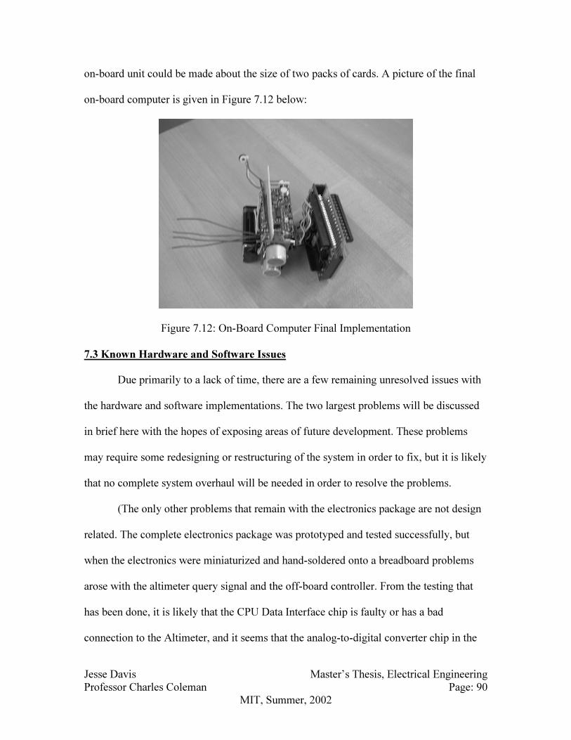
Jesse Davis Master’s Thesis, Electrical Engineering
Professor Charles Coleman Page: 90
MIT, Summer, 2002
on-board unit could be made about the size of two packs of cards. A picture of the final
on-board computer is given in Figure 7.12 below:
Figure 7.12: On-Board Computer Final Implementation
7.3 Known Hardware and Software Issues
Due primarily to a lack of time, there are a few remaining unresolved issues with
the hardware and software implementations. The two largest problems will be discussed
in brief here with the hopes of exposing areas of future development. These problems
may require some redesigning or restructuring of the system in order to fix, but it is likely
that no complete system overhaul will be needed in order to resolve the problems.
(The only other problems that remain with the electronics package are not design
related. The complete electronics package was prototyped and tested successfully, but
when the electronics were miniaturized and hand-soldered onto a breadboard problems
arose with the altimeter query signal and the off-board controller. From the testing that
has been done, it is likely that the CPU Data Interface chip is faulty or has a bad
connection to the Altimeter, and it seems that the analog-to-digital converter chip in the

Jesse Davis Master’s Thesis, Electrical Engineering
Professor Charles Coleman Page: 91
MIT, Summer, 2002
off-board controller might also be faulty or have a bad connection with the A2D
Controller. Since the prototypes worked perfectly, these two problems are considered of
minor importance, and could easily be fixed by either finding the faulty chips or
connections or rebuilding the electronics as described in the design and construction
section.)
The first major issue is that the altitude, attitude, and yaw controllers have not
been implemented in the on-board CPU code. Since the controllers have already been
derived and simulated, this will hopefully not be a major addition. Different components
of the voltages to the motors must be compensated using different controllers, however,
and so it seems that the controllers must be implemented in software and not more easily
in off-CPU hardware. In order to implement the lead controllers in software a miniature
ordinary differential equation computing engine must be implemented. Though this can
be accomplished rather easily, it is unclear whether this method will be sufficient to
successfully control the dynamics of the craft.
The second major remaining issue has to do with the interrupt processing
capabilities of the TT8. The main interrupts that the TT8 has to handle are from the Outer
Hoop Rotation Rate Sensor, the Altimeter, and the periodic interrupts required to
dynamically change the motor voltages as the motors rotate around the hub. The most
frequent of these interrupts is the periodic interrupt to change motor voltages, and the
period of this interrupt is set in the code to be 20 times faster than the Outer Hoop
Rotation Rate Sensor interrupt. When the hoop is spinning slowly with respect to the hub
(<2Hz), the operation of the CPU is perfect. When the hoop spins fast, however, the CPU
stops collecting data from the off-board controller and the Pitch, Roll, Yaw Sensor – the

Jesse Davis Master’s Thesis, Electrical Engineering
Professor Charles Coleman Page: 92
MIT, Summer, 2002
non-interrupt-driven sensors. The likely cause of this problem is that the CPU becomes
overloaded with the periodic interrupt requests to change the motor voltages. Probably
the best solution to this problem would be to design a second CPU into the system. This
second CPU would take steering commands from the main data collection CPU and
translate them into dynamic motor voltages. The second CPU could also be programmed
with the compensation and control methodologies for the system. Since specialized PID
control chips exist that would have this capability, both of the remaining implementation
problems could be solved at the same time if this additional CPU were implemented.

Jesse Davis Master’s Thesis, Electrical Engineering
Professor Charles Coleman Page: 93
MIT, Summer, 2002
8.0 Conclusion
The theory, simulation, and design of a control system for a radically new type of
flying device have been demonstrated. Control methodologies were developed from the
theoretical physical dynamics of the craft, and a complete wireless user interface system
and on-board computer were constructed and programmed to implement these
methodologies. Furthermore, it has been demonstrated by means of numerical simulation
that the control methodologies derived are viable if the actual craft were to be built.
Finally, all remaining issues with the current system implementation have been described
and suggestions for solution have been given. The primary work that remains to be done
in order to create a fully developed flying craft is to build the airframe along with
mounted motors and propellers, and interface these mechanics with the existing
electronics.
Besides simply completing the construction of the craft, there are many
possibilities for future work on this craft design. First, the hoop has not been
aerodynamically designed in order to maximize the downward thrust of the propellers.
Second, the air flow around the propellers themselves has not been investigated, but since
each propeller is constantly in the backwash of the preceding propeller, it is possible that
an entirely new propeller design would make for a more efficiently controlled craft.
Third, the efficiency of the design has not been investigated, but for any realistic use, this
would be an imperative study. Fourth, the scalability of the design has not been
investigated, so no realistic physical size limitations either large or small have been
discussed. Fifth, a non-linear state-space model based control methodology has not been
derived for this type of craft, only a vastly simplified control methodology was used.

Jesse Davis Master’s Thesis, Electrical Engineering
Professor Charles Coleman Page: 94
MIT, Summer, 2002
Sixth, GPS could be added to the craft, and more complicated types of autonomous
behavior could be developed. There are undoubtedly more possibilities for future study
surrounding this project, the ones listed here are merely to point out how broad of an
academic arena can be opened by this new type of craft design.
The possibilities for future uses of this craft make a similarly open ended list.
Constellations of the craft could be used in wide area dynamic remote surveillance
systems; the craft could be part of a Russian doll type tiered multi-vehicle reconnaissance
or delivery system; the hoop of the craft could be enlarged and hollowed to be filled with
lighter-than-air gasses in order to create a hybrid light-weight, highly maneuverable
flying device. The field of UAV research is rapidly gaining more and more attention, and
with this attention comes a responsibility to deliver meaningful advances in aerial
capabilities. Trying new types of vehicle design, regardless of their eventual
implementation into mass production, is a necessary expansion of these aerial
capabilities. Real progress rarely comes from simply re-inventing the already invented.
Instead, pushing back the boundaries of what has been done and what can be done will
prove to advance human knowledge at a far more rapid pace. Creativity and an open
mind are vital and indispensable keys to unlocking the potential of the future.

Jesse Davis Master’s Thesis, Electrical Engineering
Professor Charles Coleman Page: 95
MIT, Summer, 2002
9.0 References
1: Blaurock et al. The MIT Entry into the 1998 AUVS International Aerial Robotics
Competition. The MIT Aerial Robotics Club. 1998.
2: Borenstein, Johann. TheHoverBot – An Electrically Powered Flying Robot.
Unpublished white paper. Advanced Technologies Lab, University of Michigan:
Ann Arbor.
3: Frazzoli, Emilio; Dahleh, Munther; Feron, Eric. Robust Hybrid Control for
Autonomous Vehicle Motion Planning.
4: Gavrilets, V.; Frazzoli, E.; Mettler, B.; Piedmonte, M.; Feron, E. Aggressive
Maneuvering of Small Autonomous Helicopters: A Human-Centered Approach.
2001.
5: Gavrilets, G.; Mettler, B.; Feron, E. Dynamic Model for X-Cell 60 Helicopter in Low
Advance Ratio Flight. 2002.
6: Gavrilets, V.; Mettler, B.; Feron, E. Nonlinear Model for a Small-Size Acrobatic
Helicopter. AIAA Guidance, Navigation, and Control Conference and Exhibit,
August, 2001.
7: Gavrilets, V.; Shterenberg, A.; Dahleh, M.A.; Feron, E. Avionics System for a Small
Unmanned Helicopter Performing Aggressive Maneuvers. Massachusetts Institute
of Technology.
8: Gessow, A.; Myers, G. C. Aerodynamics of the Helicopter. F. Ungar, New York, 1967.
9: Gould, L.A.; Markey, W.R.; Roberge, J.K.; Trumper, D.L. Control Systems Theory.
Massachusetts Institute of Technology, rev. 2. 1997.
10: Jermyn et al. Helicopter with a Gyroscopic Rotor and Rotor Propellers to Provide
Vectored Thrust. United States Patent #:5,971,320. 1997.
11: Johnson, E.N.; DeBitetto, P.A.; Trott, C.A.; Bosse, M. C. The 1996 MIT / Boston
University / Draper Laboratory Autonomous Helicopter System. Draper
Laboratory, Massachusetts Institute of Technology, and Boston University.
12: Johnson, Eric; Fontaine, Sébastien; Kahn, Aaron. Minimum Complexity Uninhabited
Air Vehicle Guidance and Flight Control System. School of Aerospace
Engineering, Georgia Institute of Technology and Naval Research Laboratory.
13: Landau, L.D.; Lifshitz, E.M. Mechanics. Course of Theoretical Physics, vol. 1, ed. 3.
Institute of Physical Problems, USSR Academy of Sciences. Butterworth
Heinemann, 1976.

Jesse Davis Master’s Thesis, Electrical Engineering
Professor Charles Coleman Page: 96
MIT, Summer, 2002
14: Lundberg, Kent. Control and Tangents for Feedback Systems. Department of
Electrical Engineering, Massachusetts Institute of Technology, ver. 2.1. 2001.
15: Mettler, B.; Kanade, T.; Gavrilets, V.; Feron, E. Flight-Test Evaluation of Dynamic
Compensation for High-Bandwidth Control of Small-Scale Helicopter. AIAA
American Helicopter Society, Aerodynamics, Acoustics and Test and Evaluation.
Technical Specialist Meeting, January, 2002.
16: Morari, M.; Farruggio, David; Chapuis, Jacques. Fligende Plattform. Institut für
Automatic. 1998.
17: Neamen, Donald. Electronic Circuit Analysis and Design. ed. 2. McGraw Hill, 2001.
18: Shim, Hyunchul. Hierarchical Flight Control System Synthesis for Rotorcraft-based
Unmanned Aerial Vehicles. PhD Dissertation. Department of Mechanical
Engineering, University of California: Berkeley. 2000.
19: Shim, Hyunchul; Kim, Hyoun; Sastry, Shankar. Control System Design for
Rotorcraft-based Unmanned Aerial Vehicles using Time-domain System
Identification. Department of Mechanical Engineering, University of California:
Berkeley.
20: Shim, H.; Koo, T.J.; Hoffmann, F.; Sastry, S. A Comprehensive Study of Control
Design for an Autonomous Helicopter. Robotics and Intelligent Machines
Laboratory, University of California: Berkeley.
21: Sprague, K.; Gavrilets, V.; Dugail, D.; Mettler, B.; Feron, E.; Martinos, I. Design and
Applications of an Avionics System for a Miniature Acrobatic Helicopter.
Massachusetts Institute of Technology and Tufts University.
22: Young, Larry A. Vertical Lift – Not Just for Terrestrial Flight. Ames Research
Center, Army / NASA Rotorcraft Division.
23: Yudilevitch, G.; Levine, W.S. Techniques for Designing Rotorcraft Control Systems.
Institute for Systems Research, University of Maryland: College Park. 1994.

Jesse Davis Master’s Thesis, Electrical Engineering
Professor Charles Coleman Page: 97
MIT, Summer, 2002
10.0 Appendices
10.1 Appendix A: Matlab Simulation Code
10.1.1 State-Space Description and Step Responses
function dstatedt = state_eqns_alt(t,state); %the pitch and roll control is not working properly dstatedt = zeros(34,1); % the following command can be run at a matlab prompt once the file state_eqns.m % is saved into the directory from which matlab is launched: % % ode45('state_eqns_alt',[0 50],zeros(1,34),odeset('OutputSel',[15])) % % syntax: ode45('function',[time_start time_stop],["initial condition vector"],options) % the OutputSel selects which states are plotted , state 12 is z position % state = (b, a, i, c, tz, wx, wy, wz, wi, x, y, z, vx, vy, vz, i1, i2, i3, i4, b1, b2, b3, b4) % 1 2 3 4 5 6 7 8 9 10 11 12 13 14 15 16 17 18 19 20 21 22 23 % b,a,i,c are angles around x,y,z earth-based axes % tz is the angle around the craft-based z-axis % wx,wy,wz are angular velocities of the hoop in craft-based frame % wi is the angular velocity of the hub in the craft-based frame % x,y,z are position of craft in earth-based frame % vx,vy,vz are velocities of craft in earth-based frame % i1,i2,i3 are propeller motor currents % b1,b2,b3 are propeller angular velocities % i4,b4 are the yaw motor current and angular velocity b = state(1)*pi/180; a = state(2)*pi/180; i = state(3)*pi/180; c = state(4)*pi/180; tz = state(5)*pi/180; wx = state(6)*pi/30; wy = state(7)*pi/30; wz = state(8)*pi/30; wi = state(9)*pi/30; x = state(10); y = state(11); z = state(12); vx = state(13); vy = state(14); vz = state(15); i1 = state(16); i2 = state(17); i3 = state(18); i4 = state(19); b1 = state(20)*pi/30; b2 = state(21)*pi/30; b3 = state(22)*pi/30; b4 = state(23)*pi/30; db4dt = state(24)*pi/30; f1 = state(25); f2 = state(26); f3 = state(27); offset = state(28); Vc4 = state(29); steering = state(30); wxr = state(31)*pi/30;
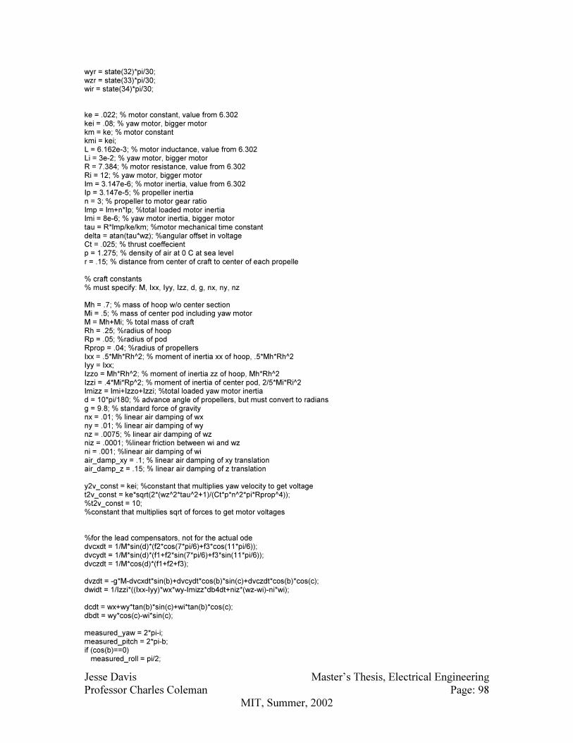
Jesse Davis Master’s Thesis, Electrical Engineering
Professor Charles Coleman Page: 98
MIT, Summer, 2002
wyr = state(32)*pi/30; wzr = state(33)*pi/30; wir = state(34)*pi/30; ke = .022; % motor constant, value from 6.302 kei = .08; % yaw motor, bigger motor km = ke; % motor constant kmi = kei; L = 6.162e-3; % motor inductance, value from 6.302 Li = 3e-2; % yaw motor, bigger motor R = 7.384; % motor resistance, value from 6.302 Ri = 12; % yaw motor, bigger motor Im = 3.147e-6; % motor inertia, value from 6.302 Ip = 3.147e-5; % propeller inertia n = 3; % propeller to motor gear ratio Imp = Im+n*Ip; %total loaded motor inertia Imi = 8e-6; % yaw motor inertia, bigger motor tau = R*Imp/ke/km; %motor mechanical time constant delta = atan(tau*wz); %angular offset in voltage Ct = .025; % thrust coeffecient p = 1.275; % density of air at 0 C at sea level r = .15; % distance from center of craft to center of each propelle % craft constants % must specify: M, Ixx, Iyy, Izz, d, g, nx, ny, nz Mh = .7; % mass of hoop w/o center section Mi = .5; % mass of center pod including yaw motor M = Mh+Mi; % total mass of craft Rh = .25; %radius of hoop Rp = .05; %radius of pod Rprop = .04; %radius of propellers Ixx = .5*Mh*Rh^2; % moment of inertia xx of hoop, .5*Mh*Rh^2 Iyy = Ixx; Izzo = Mh*Rh^2; % moment of inertia zz of hoop, Mh*Rh^2 Izzi = .4*Mi*Rp^2; % moment of inertia of center pod, 2/5*Mi*Ri^2 Imizz = Imi+Izzo+Izzi; %total loaded yaw motor inertia d = 10*pi/180; % advance angle of propellers, but must convert to radians g = 9.8; % standard force of gravity nx = .01; % linear air damping of wx ny = .01; % linear air damping of wy nz = .0075; % linear air damping of wz niz = .0001; %linear friction between wi and wz ni = .001; %linear air damping of wi air_damp_xy = .1; % linear air damping of xy translation air_damp_z = .15; % linear air damping of z translation y2v_const = kei; %constant that multiplies yaw velocity to get voltage t2v_const = ke*sqrt(2*(wz^2*tau^2+1)/(Ct*p*n^2*pi*Rprop^4)); %t2v_const = 10; %constant that multiplies sqrt of forces to get motor voltages %for the lead compensators, not for the actual ode dvcxdt = 1/M*sin(d)*(f2*cos(7*pi/6)+f3*cos(11*pi/6)); dvcydt = 1/M*sin(d)*(f1+f2*sin(7*pi/6)+f3*sin(11*pi/6)); dvczdt = 1/M*cos(d)*(f1+f2+f3); dvzdt = -g*M-dvcxdt*sin(b)+dvcydt*cos(b)*sin(c)+dvczdt*cos(b)*cos(c); dwidt = 1/Izzi*((Ixx-Iyy)*wx*wy-Imizz*db4dt+niz*(wz-wi)-ni*wi); dcdt = wx+wy*tan(b)*sin(c)+wi*tan(b)*cos(c); dbdt = wy*cos(c)-wi*sin(c); measured_yaw = 2*pi-i; measured_pitch = 2*pi-b; if (cos(b)==0) measured_roll = pi/2;

Jesse Davis Master’s Thesis, Electrical Engineering
Professor Charles Coleman Page: 99
MIT, Summer, 2002
else measured_roll = atan(tan(c)/cos(b)); end % motor constants % must specify: ke, kei, kt, kti, L, Li, R, Ri, Imp, Im, Ct, p, r % dynamic control % must specify: Vc1, Vc2, Vc3, Vc min_offset = 0; max_steering_to_offset_ratio = .75; pitch_gain = .05; roll_gain = pitch_gain; steering_tau = 50; steering_alpha = 10; steering_gain = 10; direction_gain = .7; yaw_dgain = 1000; yaw_tau = .0015; yaw_alpha = 10; alt_dgain = .00025; alt_tau = .015; alt_alpha = 10; dalt_dgoaldt = 0; dyaw_dgoaldt = 0; if (t < 5) %10 alt_dgoal = 0;%1; yaw_dgoal = 0; elseif (t < 10) %20 alt_dgoal = 0;%2; yaw_dgoal = 0; elseif (t<15) %30 alt_dgoal = 0;%-1; yaw_dgoal = 0; elseif (t<20) %40 alt_dgoal = 0; yaw_dgoal = 0; else alt_dgoal = 0; yaw_dgoal = 0; end yaw_dgoal = yaw_dgoal*pi/30; %convert to rpm goal from rad/sec goal dVc4dt = (yaw_alpha*yaw_dgain*(dwidt-dyaw_dgoaldt)+1/yaw_tau*(yaw_dgain*(wi-yaw_dgoal)-Vc4))*y2v_const; doffsetdt = alt_alpha*alt_dgain*(dalt_dgoaldt-dvzdt)+1/alt_tau*(alt_dgain*(alt_dgoal-vz)-offset); if (offset < min_offset) offset = min_offset; end dpitch_goaldt = 0; droll_goaldt = 0; if (t < 5) pitch_goal = 0*pi/180; roll_goal = 0*pi/180; elseif (t < 80) pitch_goal = 5*pi/180; roll_goal = 5*pi/180; elseif (t < 11)

Jesse Davis Master’s Thesis, Electrical Engineering
Professor Charles Coleman Page: 100
MIT, Summer, 2002
pitch_goal = 0*pi/180; roll_goal = 0*pi/180; elseif (t < 13) pitch_goal = 0*pi/180; roll_goal = 0*pi/180; else pitch_goal = 0*pi/180; roll_goal = 0*pi/180; end tilt_goal = acos(cos(pitch_goal)*cos(roll_goal)); if (roll_goal == 0) direction_goal = 0; elseif (roll_goal > 0) direction_goal = atan(tan(pitch_goal)/tan(roll_goal))-pi/2; else direction_goal = pi + atan(tan(pitch_goal)/tan(roll_goal))-pi/2; end pitch_steering = pitch_gain*(pitch_goal-measured_pitch); roll_steering = roll_gain*(roll_goal-measured_roll); if (t < 5) dsteeringdt = 0; else dsteeringdt = 2/sqrt(pitch_steering^2+roll_steering^2)*(pitch_steering*(pitch_gain*(dpitch_goaldt-(-dbdt)))+roll_steering*(roll_gain*(droll_goaldt-1/(cos(b)^2+tan(c)^2)*(cos(b)*sec(c)^2*dcdt+sin(b)*tan(c)*dbdt)))); end if (roll_steering == 0) direction = pi/2; elseif (roll_steering < 0) direction = pi+atan(pitch_steering/roll_steering); elseif (roll_steering > 0) if (pitch_steering >= 0) direction = atan(pitch_steering/roll_steering); else direction = 2*pi+atan(pitch_steering/roll_steering); end end %dsteeringdt = 0; %if (t < 5) % steering = 0; %else % steering = steering_gain*(tilt_goal - acos(cos(c)*cos(b))); %end %if (b == 0) % direction = direction_gain*direction_goal; %elseif (b > 0) % direction = direction_gain*(direction_goal-(atan(tan(measured_pitch)/tan(measured_roll)) - pi/2)); %else % direction = direction_gain*(direction_goal-(pi + atan(tan(measured_pitch)/tan(measured_roll)) - pi/2)); %end if (steering > max_steering_to_offset_ratio*offset) steering = max_steering_to_offset_ratio*offset; elseif (steering < -max_steering_to_offset_ratio*offset) steering = -max_steering_to_offset_ratio*offset; end Vc1 = sqrt(offset + steering/r/cos(d)*cos(tz-direction+delta))*t2v_const; Vc2 = sqrt(offset + steering/sqrt(3)/r/cos(d)*cos(tz-direction+delta-pi/2))*t2v_const;

Jesse Davis Master’s Thesis, Electrical Engineering
Professor Charles Coleman Page: 101
MIT, Summer, 2002
Vc3 = sqrt(offset + steering/sqrt(3)/r/cos(d)*cos(tz-direction+delta+pi/2))*t2v_const; % motor equations f1 = Ct*p*pi*r^4*n^2*b1^2; f2 = Ct*p*pi*r^4*n^2*b2^2; f3 = Ct*p*pi*r^4*n^2*b3^2; Ve1 = ke*b1; Ve2 = ke*b2; Ve3 = ke*b3; Ve4 = kei*b4; Va1 = Vc1-Ve1; Va2 = Vc2-Ve2; Va3 = Vc3-Ve3; Va4 = Vc4-Ve4; di1dt = (Va1-R*i1)/L; di2dt = (Va2-R*i2)/L; di3dt = (Va3-R*i3)/L; di4dt = (Va4-Ri*i4)/Li; m1 = km*i1; m2 = km*i2; m3 = km*i3; m4 = kmi*i4; dm4dt = kmi*di4dt; db1dt = m1/Imp; db2dt = m2/Imp; db3dt = m3/Imp; db4dt = m4/Imizz; d2b4dt2 = dm4dt/Imizz; df1dt = 2*Ct*p*pi*r^4*n^2*b1*db1dt; df2dt = 2*Ct*p*pi*r^4*n^2*b2*db2dt; df3dt = 2*Ct*p*pi*r^4*n^2*b3*db3dt; % craft equations dwxrdt = 1/Ixx*((Iyy-Izzo)*wy*wz+sin(d)*Imp*(db2dt*cos(7*pi/6)+db3dt*cos(11*pi/6))+r*cos(d)*(f2*sin(2*pi/3)+f3*sin(4*pi/3))-nx*wx); dwyrdt = 1/Iyy*((Izzo-Ixx)*wx*wz+sin(d)*Imp*(db1dt+db2dt*sin(7*pi/6)+db3dt*sin(11*pi/6))-r*cos(d)*(f1+f2*cos(2*pi/3)+f3*cos(4*pi/3))-ny*wy); dwzrdt = 1/Izzo*((Ixx-Iyy)*wx*wy+Imizz*db4dt+cos(d)*Imp*(db1dt+db2dt+db3dt)+r*sin(d)*(f1+(f2+f3)*sin(pi/2))-nz*wz-niz*(wz-wi)); dwirdt = 1/Izzi*((Ixx-Iyy)*wx*wy-Imizz*db4dt+niz*(wz-wi)-ni*wi); dwxdt = cos(tz)*dwxrdt+sin(tz)*dwyrdt-sin(tz)*wxr*wz+cos(tz)*wyr*wz; dwydt = -sin(tz)*dwxrdt+cos(tz)*dwyrdt-cos(tz)*wxr*wz-sin(tz)*wyr*wz; dwzdt = dwzrdt; dwidt = dwirdt; dtxdt = wx; dtydt = wy; dtzdt = wz; dtidt = wi; %german's: dcdt = wx+wy*tan(b)*sin(c)+wi*tan(b)*cos(c); dbdt = wy*cos(c)-wi*sin(c); dadt = wy*sin(c)/cos(b)+wz*cos(c)/cos(b); didt = wy*sin(c)/cos(b)+wi*cos(c)/cos(b); dvcxdt = 1/M*sin(d)*(f2*cos(7*pi/6)+f3*cos(11*pi/6));

Jesse Davis Master’s Thesis, Electrical Engineering
Professor Charles Coleman Page: 102
MIT, Summer, 2002
dvcydt = 1/M*sin(d)*(f1+f2*sin(7*pi/6)+f3*sin(11*pi/6)); dvczdt = 1/M*cos(d)*(f1+f2+f3); dvxdt = dvcxdt*cos(a)*cos(b)+dvcydt*(cos(a)*sin(b)*sin(c)-sin(a)*cos(c))+dvczdt*(cos(a)*sin(b)*cos(c)+sin(a)*sin(c)); dvydt = dvcxdt*sin(a)*cos(b)+dvcydt*(sin(a)*sin(b)*sin(c)+cos(a)*cos(c))+dvczdt*(sin(a)*sin(b)*cos(c)-cos(a)*cos(c)); dvzdt = -g*M-dvcxdt*sin(b)+dvcydt*cos(b)*sin(c)+dvczdt*cos(b)*cos(c); %dvxdt = 1/M*(-(f1+f2+f3)*cos(d)*sin(b)+(f2*cos(7*pi/6)+f3*cos(11*pi/6))*sin(d)*cos(i)*cos(b)+(f1+f2*sin(7*pi/6)+f3*sin(11*pi/6))*sin(d)*sin(i)*cos(b) - air_damp_xy*vx); %dvydt = 1/M*((f1+f2+f3)*cos(d)*cos(b)*sin(c)+(f2*cos(7*pi/6)+f3*cos(11*pi/6))*sin(d)*(cos(i)*sin(b)*sin(c)-sin(i)*cos(c))+(f1+f2*sin(7*pi/6)+f3*sin(11*pi/6))*sin(d)*(cos(i)*cos(c)+sin(i)*sin(b)*sin(c)) - air_damp_xy*vy); %dvzdt = 1/M*(-g*M+(f1+f2+f3)*cos(d)*cos(b)*cos(c)+(f2*cos(7*pi/6)+f3*cos(11*pi/6))*sin(d)*(cos(i)*sin(b)*cos(c)+sin(i)*sin(c))+(f1+f2*sin(7*pi/6)+f3*sin(11*pi/6))*sin(d)*(sin(i)*sin(b)*cos(c)-cos(i)*sin(c)) - air_damp_z*vz); %dvxdt = cos(a)*temp_dvxdt+sin(a)*temp_dvydt; %dvydt = -sin(a)*temp_dvxdt+cos(a)*temp_dvydt; dxdt = vx; dydt = vy; dzdt = vz; %this creates a fake ground at z = 0 if (z<=0)&(vz<=0) dzdt = 0; if (dvzdt <= 0) dvzdt = -vz*100; end end % dstatedt = d(c, b, a, i, tz, wx, wy, wz, wi, x, y, z, vx, vy, vz, i1, i2, i3, i4, b1, b2, b3, b4)dt % 1 2 3 4 5 6 7 8 9 10 11 12 13 14 15 16 17 18 19 20 21 22 2 dstatedt(1) = dbdt*180/pi; dstatedt(2) = dadt*180/pi; dstatedt(3) = didt*180/pi; dstatedt(4) = dcdt*180/pi; dstatedt(5) = dtzdt*180/pi; dstatedt(6) = dwxdt*30/pi; dstatedt(7) = dwydt*30/pi; dstatedt(8) = dwzdt*30/pi; dstatedt(9) = dwidt*30/pi; dstatedt(10) = dxdt; dstatedt(11) = dydt; dstatedt(12) = dzdt; dstatedt(13) = dvxdt; dstatedt(14) = dvydt; dstatedt(15) = dvzdt; dstatedt(16) = di1dt; dstatedt(17) = di2dt; dstatedt(18) = di3dt; dstatedt(19) = di4dt; dstatedt(20) = db1dt*30/pi; dstatedt(21) = db2dt*30/pi; dstatedt(22) = db3dt*30/pi; dstatedt(23) = db4dt*30/pi; dstatedt(24) = d2b4dt2*30/pi; dstatedt(25) = df1dt; dstatedt(26) = df2dt; dstatedt(27) = df3dt; dstatedt(28) = doffsetdt; dstatedt(29) = dVc4dt; dstatedt(30) = dsteeringdt; dstatedt(31) = dwxrdt*30/pi; dstatedt(32) = dwyrdt*30/pi; dstatedt(33) = dwzrdt*30/pi; dstatedt(34) = dwirdt*30/pi;

Jesse Davis Master’s Thesis, Electrical Engineering
Professor Charles Coleman Page: 103
MIT, Summer, 2002
10.1.2 Effects of Discretization of Dynamic Motor Voltages on Steering Control
function [avg_length,avg_angle,torque_range_factor,angle_range] = steering(discretizations,r,angle) %to execute: [l,a,f,r] = steering(25,2,0) % discretizations - number of pwm changes per revolution % r - length of desired torque vector % angle - angle of desired torque vector %r = 2; start = -2*pi; stop = 2*pi; step = .01; min = 3; max = min+2*r; offset = (max-min)/2+min; angle = angle*pi/180; min_mot = 0; t = [0 -1.5302 -1.0726 -0.7675 -0.6357 -0.5230 -0.4467 -0.3936 -0.3484 -0.3139 -0.2854 -0.2616 -0.2403 -0.2237 -0.2087 -0.1963 -0.1833 -0.1739 -0.1659 -0.1569 -0.1490 -0.1429 -0.1367 -0.1308 -0.1258 -0.1202 -0.1162 -0.1118 -0.1068 -0.1040 -0.1013 -0.0979 -0.0958 -0.0918 -0.0890 -0.0869 -0.0833 -0.0828 -0.0803 -0.0784 -0.0765 -0.0741 -0.0731 -0.0713 -0.0691 -0.0683 -0.0670 -0.0655 -0.0639 -0.0628]; n = [ 0 0.6359 0.8266 0.9001 0.9354 0.9548 0.9667 0.9744 0.9798 0.9836 0.9864 0.9886 0.9903 0.9916 0.9927 0.9936 0.9943 0.9949 0.9954 0.9959 0.9963 0.9966 0.9969 0.9971 0.9974 0.9976 0.9977 0.9979 0.9980 0.9982 0.9983 0.9984 0.9985 0.9986 0.9987 0.9987 0.9988 0.9989 0.9989 0.9990 0.9990 0.9991 0.9991 0.9991 0.9992 0.9992 0.9993 0.9993 0.9993 0.9993]; offset_angle = t(discretizations); %empirical angle offset angle = angle + offset_angle; pre_amp = 1/n(discretizations); %empirical pre-amplification r = r*pre_amp; t1 = zeros(1,floor((stop-start)/step+1)); t2 = zeros(1,floor((stop-start)/step+1)); t3 = zeros(1,floor((stop-start)/step+1)); rx = zeros(1,floor((stop-start)/step+1)); ry = zeros(1,floor((stop-start)/step+1)); j = 0; disc_step = 2*pi/discretizations; for i = start:step:stop index = round((i-start)/step) + 1; if ((i-start)/disc_step>j+1) j=j+1; end t1_tmp = offset + r*sin(start+j*disc_step-angle+pi/2); if (t1_tmp > max) t1(index) = max; elseif (t1_tmp < min) t1(index) = min; else t1(index) = t1_tmp; end t2_tmp = offset + r/sqrt(3)*sin(start+j*disc_step-angle+pi); if (t2_tmp > max) t2(index) = max;

Jesse Davis Master’s Thesis, Electrical Engineering
Professor Charles Coleman Page: 104
MIT, Summer, 2002
elseif (t2_tmp < min) t2(index) = min; else t2(index) = t2_tmp; end t3_tmp = offset + r/sqrt(3)*sin(start+j*disc_step-angle); if (t3_tmp > max) t3(index) = max; elseif (t3_tmp < min) t3(index) = min; else t3(index) = t3_tmp; end %calculate r components rx(index) = t1(index)*cos(i)+t2(index)*cos(i+2*pi/3)+t3(index)*cos(i+4*pi/3); ry(index) = t1(index)*sin(i)+t2(index)*sin(i+2*pi/3)+t3(index)*sin(i+4*pi/3); end figure(1); hold off; plot(rx,ry,'k'); axis([-r*1.25 r*1.25 -r*1.25 r*1.25]); hold on; mx = mean(rx); my = mean(ry); plot(mx,my,'ko'); %put a spot at the average legend('variation','average'); title('polar plot of torque vector variation resulting from discretizations'); xlabel('calculated torque magnitude, Nm'); ylabel('calculated torque magnitude, Nm'); hold off; i = start:step:stop; i = i.*180/pi; figure(2); hold off; plot(i,t1,'k-'); hold on; plot(i,t2,'k-.'); plot(i,t3,'k:'); legend('motor 1','motor 2','motor 3',3); title('actual discretized torque required by motors'); xlabel('angle, degrees'); ylabel('torque, Nm'); hold off; avg_angle = atan(my/mx)*180/pi; %check to see if the angle was met avg_length = sqrt(mx^2+my^2); %check to see if the length was met torque_range_factor = max/min; %factor over which the motor speed must change per cycle from min to max sorted = sort(ry); miny = sorted(1); maxy = sorted(length(sorted)); angle_range = (atan(maxy/mx)-atan(miny/mx))*180/pi; figure(3); angles = [ 115.0743 95.9820 76.2684 64.8416 55.2586 48.5117 42.8720 38.5602 34.8101 31.8759 29.3216 27.0291 25.2744 23.6231 22.2078 20.9263 19.7947 18.7594 17.8198 16.9988 16.2327 15.5578 14.9054 14.2967 13.7014 13.2688 12.7823 12.1945 11.9398 11.5729 11.2129 10.8554 10.5368 10.2465 9.9687 9.7037 9.4451 9.1638 8.9716 8.7563 8.5342 8.3529 8.1465 7.9811 7.8138 7.6477 7.4852 7.3351 7.1856]; i = 2:50; plot(i,angles,'k'); xlabel('discretizations'); ylabel('total angle of torque variation, degrees'); title('total angle of torqe variation over time vs. discretizations');
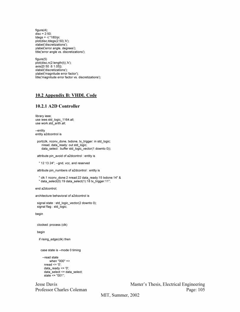
Jesse Davis Master’s Thesis, Electrical Engineering
Professor Charles Coleman Page: 105
MIT, Summer, 2002
figure(4); disc = 2:50; tdegs = -t.*180/pi; plot(disc,tdegs(2:50),'k'); xlabel('discretizations'); ylabel('error angle, degrees'); title('error angle vs. discretizations'); figure(5) plot(disc,n(2:length(t)),'k'); axis([0 50 .6 1.05]); xlabel('discretizations'); ylabel('magnitude error factor'); title('magnitude error factor vs. discretizations');
10.2 Appendix B: VHDL Code
10.2.1 A2D Controller
library ieee; use ieee.std_logic_1164.all; use work.std_arith.all; --entity entity a2dcontrol is port(clk, nconv_done, txdone, tx_trigger: in std_logic; nread, data_ready: out std_logic; data_select : buffer std_logic_vector(1 downto 0)); attribute pin_avoid of a2dcontrol : entity is " 12 13 24"; --gnd, vcc, and reserved attribute pin_numbers of a2dcontrol : entity is " clk:1 nconv_done:2 nread:22 data_ready:15 txdone:14" & " data_select(0):19 data_select(1):18 tx_trigger:11"; end a2dcontrol; architecture behavioral of a2dcontrol is signal state : std_logic_vector(2 downto 0); signal flag : std_logic; begin clocked: process (clk) begin if rising_edge(clk) then case state is --mode 0 timing --read state when "000" => nread <= '0'; data_ready <= '0'; data_select <= data_select; state <= "001";

Jesse Davis Master’s Thesis, Electrical Engineering
Professor Charles Coleman Page: 106
MIT, Summer, 2002
--allow a2d time to respond when "001" => nread <= '0'; data_ready <= '0'; data_select <= data_select; state <= "010"; --wait for data to be ready when "010" => if (nconv_done = '1') then state <= "010"; else state <= "011"; end if; nread <= '0'; data_ready <= '0'; data_select <= data_select; --wait for rising tx_trigger / let ser_send know data is ready --and allow for valid data delay out of a2d when "011" => if (tx_trigger = '1') then if (flag = '1') then data_ready <= '1'; state <= "100"; flag <= '0'; else data_ready <= '0'; state <= "011"; end if; else data_ready <= '0'; state <= "011"; flag <= '1'; end if; nread <= '0'; data_select <= data_select; --give ser_send time to respond with a txdone = '1' when "100" => nread <= '0'; data_ready <= '1'; state <= "101"; data_select <= data_select; --wait for ser_send to finish transmitting when "101" => if (txdone = '1') then nread <= '1'; data_ready <= '0'; state <= "110"; else nread <= '0'; data_ready <= '1'; state <= "101"; end if; data_select <= data_select; --allow for address hold time of a2d (might not need this state) when "110" => nread <= '1'; data_ready <= '0'; state <= "111"; data_select <= data_select; --change data to be sent when "111" => nread <= '1'; data_ready <= '0';

Jesse Davis Master’s Thesis, Electrical Engineering
Professor Charles Coleman Page: 107
MIT, Summer, 2002
state <= "000"; data_select <= data_select + 1; --when others go to 000 state when others => nread <= '1'; data_ready <= '0'; state <= "000"; data_select <= data_select; end case; end if; end process; end behavioral;
10.2.2 Serializer
library ieee; use ieee.std_logic_1164.all; use work.std_arith.all; entity serializer is port(clk, txbit, txdone : in std_logic; data_in : in std_logic_vector(9 downto 0); data_out : out std_logic); attribute pin_avoid of serializer : entity is " 13 "; --reserved attribute pin_numbers of serializer : entity is " clk:1 txbit:2 txdone:3 data_out:19 data_in(0):14 data_in(1):15 " & " data_in(2):4 data_in(3):5 data_in(4):6 data_in(5):7 " & " data_in(6):8 data_in(7):9 data_in(8):10 data_in(9):11 "; end serializer; architecture behavioral of serializer is signal bit_count : std_logic_vector(3 downto 0); signal flag : std_logic; begin clocked: process (clk) begin if rising_edge(clk) then if (txdone = '1') then data_out <= '0'; bit_count <= "0000"; flag <= '0'; elsif (txbit = '0') then flag <= '0';

Jesse Davis Master’s Thesis, Electrical Engineering
Professor Charles Coleman Page: 108
MIT, Summer, 2002
elsif ((txbit = '1') and (flag = '0')) then flag <= '1'; case bit_count is when "0000" => data_out <= data_in(0); --start bit, tied high bit_count <= "0001"; when "0001" => data_out <= not data_in(1); --data 0 bit_count <= "0010"; when "0010" => data_out <= not data_in(2); --data 1 bit_count <= "0011"; when "0011" => data_out <= not data_in(3); --data 2 bit_count <= "0100"; when "0100" => data_out <= not data_in(4); --data 3 bit_count <= "0101"; when "0101" => data_out <= not data_in(5); --data 4 bit_count <= "0110"; when "0110" => data_out <= not data_in(6); --select 0 bit_count <= "0111"; when "0111" => data_out <= not data_in(7); --select 1 bit_count <= "1000"; when "1000" => data_out <= not data_in(8); --mode bit_count <= "1001"; when "1001" => data_out <= data_in(9); --stop, tied low bit_count <= "1010"; when "1010" => data_out <= '0'; bit_count <= "0000"; when others => bit_count <= "0000"; end case; end if; end if; end process; end behavioral;

Jesse Davis Master’s Thesis, Electrical Engineering
Professor Charles Coleman Page: 109
MIT, Summer, 2002
10.2.3 Serializer Controller
library ieee; use ieee.std_logic_1164.all; use work.std_arith.all; --entity entity ser_send is port(clk, data_ready: in std_logic; per_counter : in std_logic_vector(3 downto 0); en_nres, txbit, txdone: out std_logic); attribute pin_avoid of ser_send : entity is " 12 13 24"; --gnd, vcc, and reserved attribute pin_numbers of ser_send : entity is " clk:1 data_ready:2 txdone:18 en_nres:20 " & " per_counter(0):5 per_counter(1):6 per_counter(2):7 " & " per_counter(3):8 txbit:14"; end ser_send; --the period counter might have to be frigged with to get the data rate --equal to that when the computer is txmitting. in this case, you could --use per_counter inputs as certain inputs that when all 1's will be the --right period, but may not be sequential bits from the counter. this will --make transition from computer control to joystick control easier architecture behavioral of ser_send is signal bit_count : std_logic_vector(3 downto 0); signal state : std_logic_vector(1 downto 0); begin clocked: process (clk) begin if rising_edge(clk) then case state is --startup when "00" => state <= "01"; txdone <= '0'; txbit <= '0'; en_nres <= '0'; bit_count <= "0000"; --wait for data to be ready when "01" => if (data_ready = '1') then state <= "10"; txdone <= '0'; txbit <= '1'; bit_count <= bit_count + 1; else state <= "01"; txdone <= '1'; txbit <= '0'; bit_count <= "0000";
Jesse Davis Master’s Thesis, Electrical Engineering
Professor Charles Coleman Page: 110
MIT, Summer, 2002
end if; en_nres <= '0'; --count period and bits when "10" => if (bit_count = "1010") then state <= "11"; txdone <= '1'; en_nres <= '0'; txbit <= '0'; bit_count <= "0000"; elsif (per_counter = "1111") then bit_count <= bit_count + 1; txbit <= '1'; state <= "10"; txdone <= '0'; en_nres <= '0'; else bit_count <= bit_count; txbit <= '0'; state <= "10"; txdone <= '0'; en_nres <= '1'; end if; --allow time for a2d to give back data_ready = 0 when "11" => state <= "01"; txdone <= '1'; en_nres <= '0'; txbit <= '0'; bit_count <= "0000"; --same as 00 when others => state <= "01"; txdone <= '0'; en_nres <= '0'; txbit <= '0'; bit_count <= "0000"; end case; end if; end process; end behavioral;
10.2.4 CPU Data Interface
library ieee; use ieee.std_logic_1164.all; use work.std_arith.all; entity alt_querrier is port(clk, serial_in_1, serial_in_2, serial_in_3 : in std_logic; querry, serial_out_1, serial_out_2, serial_out_3 : out std_logic); attribute pin_avoid of alt_querrier : entity is " 13 "; --reserved attribute pin_numbers of alt_querrier : entity is

Jesse Davis Master’s Thesis, Electrical Engineering
Professor Charles Coleman Page: 111
MIT, Summer, 2002
" clk:1 querry:22 " & " serial_in_1:2 serial_out_1:21" & " serial_in_2:3 serial_out_2:20" & " serial_in_3:4 serial_out_3:19"; end alt_querrier; architecture behavioral of alt_querrier is signal state : std_logic_vector(2 downto 0); begin serial_out_1 <= not serial_in_1; serial_out_2 <= not serial_in_2; serial_out_3 <= not serial_in_3; clocked: process (clk) begin if rising_edge(clk) then case state is when "000" => state <= "001"; querry <= '0'; when "001" => state <= "010"; querry <= '0'; when "010" => state <= "011"; querry <= '0'; when "011" => state <= "100"; querry <= '0'; when "100" => state <= "101"; querry <= '0'; when "101" => state <= "110"; querry <= '0'; when "110" => state <= "111"; querry <= '0'; when "111" => state <= "000"; querry <= '1'; when others => state <= "000"; querry <= '0'; end case; end if; end process; end behavioral;

Jesse Davis Master’s Thesis, Electrical Engineering
Professor Charles Coleman Page: 112
MIT, Summer, 2002
10.3 Appendix C: CPU Code
10.3.1 Header File
#include <tt8.h> #include <tat332.h> #include <sim332.h> #include <tpu332.h> #include <dio332.h> #include <qsm332.h> #include <tt8pic.h> #include <tt8lib.h> #include <userio.h> #include <stdio.h> #include <stdlib.h> #include <stddef.h> #include <math.h> #include <float.h> //constants #define PI 3.141593 #define G 9.8 #define CRAFT_MASS 1 //mass of total craft #define HOVER_THRUST CRAFT_MASS*G #define USPERCM 74 //microseconds per centimeter for alt echo #define MAX_ALT_ECHO_TIME 39000 //39ms, data sheet says 36ms #define MIN_ALT_ECHO_TIME 100 //100us, data sheet says 100us #define MOTOR_PWM_HI_VOLTS 20 //20 volt battery pack #define MOTOR_PWM_HI_MIN 20 //minimum amount of hi time on pwm #define MOTOR_PWM_HI_MAX 180 //maximum amount of hi time on pwm #define MOTOR_PWM_HI_STARTUP 50 //startup amount of hi time on pwm #define MOTOR_STARTUP_TIME 1000 //bring motors to startup speed in 1000 ms #define MOTOR_MIN_THRUST 3 //this can be changed or calibrated #define MOTOR_MAX_STEERING 2.5 //don't want max steering to be larger than min thrust #define MAX_STEER_TO_THRUST_RATIO .75 //don't want steering compared to thrust too large #define OUT_VOLTSSQPERNEWTON .5 //this will have to be calculated and calibrated //should theoretically be equal to 2*Ke^2/(p*r^4*PI) #define OUT_VOLTSSQPERNEWTONMETER .5 //this will also have to be calculated and calibrated //should theoretically be equal to 2*Ke^2/(p*r^5*PI) #define OUT_MOTOR_KE .2 //Ke //where Ke is the back emf motor constant, p is the density of air, and r is the radius //from the center of the vectron to the center of the motors #define USR_MAX_DATA 15 // 0b1111 = 15 #define USR_DAT2DEGREES 2 //max 30 degrees / max data of 0b1111=15 #define USR_DAT2NEWTONS .3 //.5kg*10m/s^2 = 5, max thrust data = 31, max thrust ~10 #define USR_STABLE_PITCH 0.0f #define USR_STABLE_ROLL 0.0f #define USR_STABLE_ALT_SPEED 0.0f #define USR_STABLE_YAW_SPEED 0.0f #define PRY_DAT2DEGREES 180/PI/10430 //this is given in the pry datasheet #define WZ_MILLISEC2HZ 1000 //WZ_MILLISEC2HZ/milliseconds = hertz conversion #define WZ_MAX_HZ 10 //max allowable hz output for glitch protection #define BAD_DATA -1000.0f #define ALT_SPEED_GAIN 5 //will have to be determined in simulations #define YAW_GAIN 5 //will have to be determined in simulations #define PITCH_GAIN 5 //will have to be determined in simulations

Jesse Davis Master’s Thesis, Electrical Engineering
Professor Charles Coleman Page: 113
MIT, Summer, 2002
#define ROLL_GAIN 5 //will have to be determined in simulations //define timing vars #define MOTOR_PWM_PERIOD 200 //4MHz/200 --> 20KHz PWM, 50us period #define MOTOR_PWM_DISCRETIZATIONS 20 //20 ~-> 10ms changes, 40 ~-> 5ms changes #define ALT_PWM_PERIOD 25000 //4MHz/25000 --> 160Hz PWM #define ALT_PWM_HI_TIME 12500 //datasheet says min is 10us, will be 6.25ms #define PRY_REQ_DELAY 35 //35ms between each pry request, ~28.57Hz #define WZ_TIMEOUT_DELAY 10000 //10s timeout #define ALT_TIMEOUT_DELAY 1000 //1s timeout since it's querried all the time //define pins #define TPU_USR_PIN 0 #define TPU_PRY_PIN 1 #define TPU_PRY_REQ_PIN 2 #define TPU_ALT_QUERY_PIN 3 #define TPU_ALT_ECHO_PIN 4 #define PWM_OUTPUT_PIN1 5 #define PWM_OUTPUT_PIN2 6 #define PWM_OUTPUT_PIN3 7 #define PWM_YAW_OUTPUT_PIN 8 #define TPU_WZ_PIN 9 #define A2D_USR_DETECT_PIN 0 //A2D 1, not TPU 1 //needed a 1 MOhm resistor to ground on usr detect pin #define NUM_PRIMARY_PWM_CHANNELS 3 #define PWM_CHANNEL_OFFSET 5 //define pry command and response formats #define PRY_REQ 192 //0b11000000 - 0xC0 #define PRY_RESPONSE_BYTES 7 #define PRY_VALID_HEADER 68 //0x44 //define buffer sizes for PRY and user data #define USR_BITSPERBYTE 8 #define USR_BUF_SIZE USR_BITSPERBYTE*16 //16 byte buffer #define PRY_BITSPERBYTE 8 #define PRY_BUF_SIZE PRY_BITSPERBYTE*16 //16 byte buffer #define PRY_REQ_BITSPERBYTE 8 #define PRY_REQ_BUF_SIZE PRY_REQ_BITSPERBYTE*4 //4 byte buffer //this last buffer is never used //define some macro functions #define USR_READY_FOR_UPDATE TSerByteAvail(TPU_USR_PIN) //is there usr data? #define GET_USR_BYTE TSerGetByte(TPU_USR_PIN) //get the usr data #define FLUSH_USR_DAT TSerInFlush(TPU_USR_PIN) //flush the usr data buffer
Jesse Davis Master’s Thesis, Electrical Engineering
Professor Charles Coleman Page: 114
MIT, Summer, 2002
#define PRY_READY TSerByteAvail(TPU_PRY_PIN) //is there pry data? #define PRY_READY_FOR_UPDATE ((MilliSecs() - pry_req_timer) >= PRY_REQ_DELAY) #define GET_PRY_BYTE TSerGetByte(TPU_PRY_PIN) //get the pry data #define FLUSH_PRY_DAT TSerInFlush(TPU_PRY_PIN) //flush the pry data buffer #define SEND_PRY_REQ TSerPutByte(TPU_PRY_REQ_PIN,PRY_REQ) #define ECHO TPUGetPin(TPU_ALT_ECHO_PIN) //query echo #define WZ TPUGetPin(TPU_WZ_PIN) #define USR_DETECT_MILLIV AtoDReadMilliVolts(A2D_USR_DETECT_PIN) #define PWM_READY_FOR_UPDATE (pit_counter != pit_hits) #define UPDATE_PWM \ if (PWM_READY_FOR_UPDATE) \ \ TPUUpdateAllChans(); \ pit_counter = pit_hits; \ #define UPDATE_USR \ if (USR_READY_FOR_UPDATE) \ \ usr_time = get_usr_dat(&usr_dat, 0, usr_time); \ change_output = 1; \ #define UPDATE_PRY \ if (PRY_READY_FOR_UPDATE) \ \ pry_req_timer = MilliSecs(); \ pry_time = get_pry_dat(&pry_dat, 0, pry_time); \ change_output = 1; \ #define TIMEOUT_WZ \ if ((MilliSecs() - wz_time) >= WZ_TIMEOUT_DELAY) \ \ wz_dat.wz = BAD_DATA; \ wz_dat.dwzdt = BAD_DATA; \ start_up_pwm = 1; \ SetSteeringInterruptTimer(0); \ #define TIMEOUT_ALT \ if ((MilliSecs() - alt_time) >= ALT_TIMEOUT_DELAY) \ \ alt_dat.alt = BAD_DATA; \ alt_dat.daltdt = BAD_DATA; \ #define RESTART_PWM_AFTER_WZ_TIMEOUT \ if ((wz_dat.wz != BAD_DATA) & (start_up_pwm == 1)) \ \ start_up_pwm = 0; \ #define UPDATE_OUTPUT \ if (change_output == 1) \ state_time = state_estimator(&state_dstate, &pry_dat, 0, state_time); \ controller(&state_dstate, &pry_dat, &usr_dat); \ UPDATE_PWM; \ change_output = 0; \

Jesse Davis Master’s Thesis, Electrical Engineering
Professor Charles Coleman Page: 115
MIT, Summer, 2002
//struct definitions struct USR_STRUCT int mode; //mode0 = usr control, mode1 = hover, etc... float pitch_c; //all angles are measured in degrees float roll_c; //angles are 4-bit discretized and then converted float yaw_c; float thrust_c; //measured in newtons float dpitch_cdt; //change in degrees float droll_cdt; //by the transmitter float dyaw_cdt; float dthrust_cdt; ; struct PRY_STRUCT float pitch; //want high precision from sensor, sub degree float roll; float yaw; float dpitchdt; //want high precision in derivative too float drolldt; float dyawdt; float pitch_tare; float roll_tare; float yaw_tare; ; struct ALT_STRUCT float alt; //measured in cm, range ~3-300 float daltdt; ; struct WZ_STRUCT float wz; //measured in Hz float dwzdt; ; struct STATE_STRUCT float tilt; float aparent_yaw; float actual_altitude; float dtiltdt; float daparent_yawdt; float dactual_altitudedt; ; struct OUTPUT_STRUCT float thrust_offset; //want precision on voltage to be applied to motors float pitch_roll_steering; float yaw_steering; float steering_angle; short pwm_hi_time_1; short pwm_hi_time_2; short pwm_hi_time_3; short pwm_hi_time_yaw; ; //for the pwm control /* PSC Pin State Control */ #define ForceByPAC 0x00 #define ForceHigh 0x01 #define ForceLow 0x02 #define NoForceState 0x03 /* PAC Pin Action Control (Inputs) */ #define NoTranDet 0x00 #define DetRising 0x04 #define DetFalling 0x08
Jesse Davis Master’s Thesis, Electrical Engineering
Professor Charles Coleman Page: 116
MIT, Summer, 2002
#define DetEither 0x0c #define NoChangePAC 0x10 /* PAC Pin Action Control (Outputs) */ #define NoChangematch 0x00 #define HighOnMatch 0x04 #define LowOnMatch 0x08 #define ToggleOnMatch 0x0c /* TBS Time Base/Directionality Control */ #define InputChan 0x00 #define OutputChan 0x80 #define Cap1Match1 0x00 #define Cap1Match2 0x20 #define Cap2Match1 0x40 #define Cap2Match2 0x60 #define NoChangeTBS 0x100 //function headers void init_alt_meas(void); ulong get_usr_dat(struct USR_STRUCT *usr_dat, short initialize_flag, ulong usr_time); void get_alt_dat(void); ulong get_pry_dat(struct PRY_STRUCT *pry_dat, short initialize_flag, ulong pry_time); void get_wz_dat(void); ulong state_estimator(struct STATE_STRUCT *state_dstate, struct PRY_STRUCT *pry_dat, short initialize_flag, ulong state_time); void controller(struct STATE_STRUCT *state_dstate, struct PRY_STRUCT *pry_dat, struct USR_STRUCT *usr_dat); void TPUInitPWM(short chan, short hi_time, short period); void TPUChangePWM(short chan, short hi_time, short period); void TPUUpdateAllChans(void); void InitOutputSteering(int delay); void SetSteeringInterruptTimer(int delay); void ServiceOutputSteeringInterrupt(void);
10.3.2 C Code File
#include "main.h" //THE USR DATA INPUT AND ALTIMETER NEED TO BE CALIBRATED //THE OUTPUT PWM HI TIMES NEED TO BE CALIBRATED //IF THE PERIODIC INTERRUPT TIMER GOES TOO FAST, THINGS GO AWRY ulong alt_time; //global so interrupt can access ulong wz_time; struct ALT_STRUCT alt_dat; //global so interrupt can access struct WZ_STRUCT wz_dat; struct OUTPUT_STRUCT output; int alt_dat_valid; double current_angle; int change_output; //change flag, global so interrupts can access int pit_hits; int pit_counter; void main(void) int start_up_pwm = 0; int i, j; //initialize variables

Jesse Davis Master’s Thesis, Electrical Engineering
Professor Charles Coleman Page: 117
MIT, Summer, 2002
struct USR_STRUCT usr_dat; //these structs are defined in main.h struct PRY_STRUCT pry_dat; struct STATE_STRUCT state_dstate; ptr usr_buf; ptr pry_buf; ptr pry_req_buf; ulong pry_time = 0; //initialize timers ulong pry_req_timer = 0; ulong usr_time = 0; ulong state_time = 0; static ExcCFrame efp1; //initialize interrupt frame handler static ExcCFrame efp2; static ExcCFrame efp3; //initialize tt8 InitTT8(NO_WATCHDOG, TT8_TPU); //initializes tt8 for action SimSetFSys(16000000); //sets system speed to 16MHz alt_time = 0; wz_time = 0; pit_hits = 0; pit_counter = 0; alt_dat_valid = 1; current_angle = 0; //will be initialized to zero every time the wz transitions change_output = 0; InstallHandler(get_alt_dat, TPU_INT_VECTOR + TPU_ALT_ECHO_PIN, &efp1); //setup interrupt handling InstallHandler(get_wz_dat, TPU_INT_VECTOR + TPU_WZ_PIN, &efp2); *PITR = 0; //disable periodic timer interrupt InstallHandler(ServiceOutputSteeringInterrupt, PIT_INT_VECTOR, &efp3); //initialize serial ports for usr and pry if ((usr_buf = malloc(USR_BUF_SIZE+TSER_MIN_MEM)) == 0) return; //can't allocate serial input buffer for usr commands so quit if (TSerOpen(TPU_USR_PIN,HighPrior,0,usr_buf,USR_BUF_SIZE,2400,'N',USR_BITSPERBYTE,1) != tsOK) return; //can't open channel for usr serial input //the TSER_MIN_MEM is a tt8 minimum "scratchpad" memory requirement in the buffer. //it is defined in tat332.h. all other capitalized variables are defined in main.h //initialize serial ports for pry if ((pry_buf = malloc(PRY_BUF_SIZE+TSER_MIN_MEM)) == 0) return; //can't allocate serial input buffer for pry data so quit if (TSerOpen(TPU_PRY_PIN,HighPrior,0,pry_buf,PRY_BUF_SIZE,9600,'N',PRY_BITSPERBYTE,1) != tsOK) return; //can't open channel for pry serial input //may need to adjust some of the pry serial settings once pry sensor comes in if ((pry_req_buf = malloc(PRY_REQ_BUF_SIZE+TSER_MIN_MEM)) == 0) return; //can't allocate serial input buffer for pry data so quit if (TSerOpen(TPU_PRY_REQ_PIN,HighPrior,1,pry_req_buf,PRY_REQ_BUF_SIZE,9600,'N',PRY_REQ_BITSPERBYTE,1) != tsOK) return; //can't open channel for pry serial input TPUGetPin(TPU_ALT_ECHO_PIN); //define as input pins TPUGetPin(TPU_WZ_PIN); TPUInterruptEnable(TPU_ALT_ECHO_PIN); //enable interrupts TPUInterruptEnable(TPU_WZ_PIN); SetInterruptMask(ALL_RUPTS_MASK); //tell main computer about interrupts

Jesse Davis Master’s Thesis, Electrical Engineering
Professor Charles Coleman Page: 118
MIT, Summer, 2002
//initialize motors to startup speed for (i = 0; i <= MOTOR_PWM_HI_STARTUP; i++) for (j = 0; j < NUM_PRIMARY_PWM_CHANNELS; j++) if (i == 0) TPUInitPWM(j + PWM_CHANNEL_OFFSET, i, MOTOR_PWM_PERIOD); else TPUChangePWM(j + PWM_CHANNEL_OFFSET, i, MOTOR_PWM_PERIOD); DelayMilliSecs(MOTOR_STARTUP_TIME/MOTOR_PWM_HI_STARTUP); //initialize data structures and operations, wz initialized behind the scenes sorta usr_time = get_usr_dat(&usr_dat, 1, usr_time); pry_time = get_pry_dat(&pry_dat, 1, pry_time); init_alt_meas(); DelayMilliSecs(1); //give altimeter time to respond, should be ~200us response + ~200us echo on ground state_time = state_estimator(&state_dstate, &pry_dat, 1, state_time); controller(&state_dstate, &pry_dat, &usr_dat); pry_req_timer = MilliSecs(); //main operation loop, infinite while (1) UPDATE_PRY; UPDATE_USR; UPDATE_PWM; RESTART_PWM_AFTER_WZ_TIMEOUT; TIMEOUT_WZ; TIMEOUT_ALT; UPDATE_OUTPUT; //end of while loop Reset(); //needs to be Reset() for ram programs ResetToMon() for flash return; /*************************Sub-routines follow************************/ /******************************************************************/ /* function: Initiates altimeter measurements inputs: none outputs: none */ void init_alt_meas(void) TPUInitPWM(TPU_ALT_QUERY_PIN,ALT_PWM_HI_TIME,ALT_PWM_PERIOD); return;

Jesse Davis Master’s Thesis, Electrical Engineering
Professor Charles Coleman Page: 119
MIT, Summer, 2002
/******************************************************************/ /* function: Collects the data from the user input inputs: *usr_dat - pointer to the current user data initialize_flag - tells routine whether this is the initialization usr_time - last time the user data was updated (from MilliSecs()) outputs: time - current time from MilliSecs() routine */ ulong get_usr_dat(struct USR_STRUCT *usr_dat, short initialize_flag, ulong usr_time) //assume buffered by tt8 serial port //need to know what tt8 expects for incoming serial data bits /* bit value: mode <select> +/- <- data -> bit number: 8 7 6 5 4 3 2 1 hex mask: 0x0080 0x0060 0x0010 0x000F short mask: 128 96 16 15 since there is only positive thrust, bit 5 will be data in the thrust case */ ulong elapsed_time, time; //setup variables to be their own masks to the incoming byte int mode = 128; int selector = 96; int pve_nve = 16; int data_c_tmp = 15; uchar tmp_byte; float data_c_tmp_f; float pve_nve_f; float elapsed_time_f; float usr_dat2degrees_f = USR_DAT2DEGREES; float usr_dat2newtons_f = USR_DAT2NEWTONS; //find out how much time since last update time = MilliSecs(); elapsed_time = time - usr_time; if (4050<USR_DETECT_MILLIV) //this is a safety, just in case the transmitter shuts off tmp_byte = GET_USR_BYTE; //defined above main else //this will put the vectron into a stable hover usr_dat->mode = 0; //mode 0 will be auto mode, mode 1 will be user mode usr_dat->thrust_c = BAD_DATA; //30; //will control thrust for hover in the controller usr_dat->dthrust_cdt = BAD_DATA; //0; //see thrust note one line up usr_dat->yaw_c = BAD_DATA; //current_yaw; usr_dat->dyaw_cdt = BAD_DATA; //0; usr_dat->pitch_c = BAD_DATA; //USR_STABLE_PITCH; usr_dat->dpitch_cdt = BAD_DATA; //0; usr_dat->roll_c = BAD_DATA; //USR_STABLE_ROLL; usr_dat->droll_cdt = BAD_DATA; //0; return usr_time; //receiver not receiving mode &= tmp_byte; //as initialized mode is its own mask to get the mode //data out of the received byte, all others are same mode >>= 7; //shift bit down to bottom mode &= 1; //this will erase all but bottom bit in case 1's came in top

Jesse Davis Master’s Thesis, Electrical Engineering
Professor Charles Coleman Page: 120
MIT, Summer, 2002
//of int when shift occured selector &= tmp_byte; selector >>= 5; selector &= 3; //this will erase all but the bottom two bits data_c_tmp &= tmp_byte; //no need to shift, already at bottom pve_nve &= tmp_byte; if (selector != 3) //if not thrust data, convert to +1 or -1 if (pve_nve == 0) //let 0 = -1, 1 = 1 pve_nve = -1; data_c_tmp ^= 15; //invert bits else pve_nve = 1; else //it's thrust data so tack it on to data_c_tmp data_c_tmp |= pve_nve; //change all data to floating point data data_c_tmp_f = data_c_tmp; pve_nve_f = pve_nve; elapsed_time_f = elapsed_time; //all data is now collected so lets put it in the usr_dat struct usr_dat->mode = mode; //need this syntax since usr_dat is a pointer //each byte only has info for either pitch or roll or yaw or thrust switch(selector) case 0 : if (initialize_flag == 0) //if this isn't an initialization, change d(x)dt vars usr_dat->dpitch_cdt = 1000.0f*(pve_nve_f*data_c_tmp_f*usr_dat2degrees_f - usr_dat->pitch_c)/elapsed_time_f; else usr_dat->dpitch_cdt = pve_nve_f*data_c_tmp_f*usr_dat2degrees_f; //elapsed time is in milliseconds so we need to multiply by 1000 usr_dat->pitch_c = pve_nve_f*data_c_tmp_f*usr_dat2degrees_f; //update data in usr_dat, must convert from binary number to degrees break; case 1 : if (initialize_flag == 0) usr_dat->droll_cdt = 1000.0f*(pve_nve_f*data_c_tmp_f*usr_dat2degrees_f - usr_dat->roll_c)/elapsed_time_f; else usr_dat->droll_cdt = pve_nve_f*data_c_tmp_f*usr_dat2degrees_f; usr_dat->roll_c = pve_nve_f*data_c_tmp_f*usr_dat2degrees_f; break; case 2 : if (initialize_flag == 0) usr_dat->dyaw_cdt = 1000.0f*(pve_nve_f*data_c_tmp_f*usr_dat2degrees_f - usr_dat->yaw_c)/elapsed_time_f;
Jesse Davis Master’s Thesis, Electrical Engineering
Professor Charles Coleman Page: 121
MIT, Summer, 2002
else usr_dat->dyaw_cdt = pve_nve_f*data_c_tmp_f*usr_dat2degrees_f; usr_dat->yaw_c = pve_nve_f*data_c_tmp_f*usr_dat2degrees_f; break; case 3 : if (initialize_flag == 0) usr_dat->dthrust_cdt = 1000.0f*(data_c_tmp_f*usr_dat2newtons_f - usr_dat->thrust_c)/elapsed_time_f; else usr_dat->dthrust_cdt = data_c_tmp_f*usr_dat2newtons_f; usr_dat->thrust_c = data_c_tmp_f*usr_dat2newtons_f; //update thrust, must convert from binary to newtons //no default case because selector can only be 0,1,2,3 due to the //processing we did on it above return time; /******************************************************************/ /* function: Collects the data from the pitch, roll, yaw sensor inputs: *pry_dat - pointer to the current pry data initialize_flag - tells routine whether this is the initialization pry_time - last time the pry data was updated (from MilliSecs()) outputs: time - current time from MilliSecs() routine */ ulong get_pry_dat(struct PRY_STRUCT *pry_dat, short initialize_flag, ulong pry_time) int bytes_received = 0; unsigned int pitch_tmp, yaw_tmp, header; int roll_tmp; ulong elapsed_time, time; //find out how much time since last update ulong time_out; float tmp_f, elapsed_time_f, pry_dat2degrees_f; time = MilliSecs(); elapsed_time = time - pry_time; FLUSH_PRY_DAT; //macro defined in main.h //this will be a polled operation SEND_PRY_REQ; //macro defined in main.h DelayMilliSecs(15); //15ms worst case delay between request and response from testing for (bytes_received=0; bytes_received < PRY_RESPONSE_BYTES ; bytes_received++) time_out = MilliSecs(); while (!PRY_READY) //timed out wait for data to arrive if (MilliSecs() - time_out > 5) //from testing 5ms is good time out period if (bytes_received <= 2) //if we timed out with no bytes received then the pry isn't working pry_dat->roll = BAD_DATA; pry_dat->drolldt = BAD_DATA; pry_dat->pitch = BAD_DATA;
Jesse Davis Master’s Thesis, Electrical Engineering
Professor Charles Coleman Page: 122
MIT, Summer, 2002
pry_dat->dpitchdt = BAD_DATA; pry_dat->yaw = BAD_DATA; pry_dat->dyawdt = BAD_DATA; return pry_time; UPDATE_PWM; switch(bytes_received) case 0 : header = GET_PRY_BYTE; if (header != PRY_VALID_HEADER) // defined in main.h return pry_time; //there was some error break; case 1 : roll_tmp = GET_PRY_BYTE; //get roll msb roll_tmp *= 256; //shift msb up 8 bits break; case 2 : roll_tmp += GET_PRY_BYTE; //get roll lsb break; case 3 : pitch_tmp = GET_PRY_BYTE; //get pitch msb pitch_tmp *= 256; //shift msb up 8 bits break; case 4 : pitch_tmp += GET_PRY_BYTE; //get pitch lsb break; case 5 : yaw_tmp = GET_PRY_BYTE; //get yaw msb yaw_tmp *= 256; //shift msb up 8 bits break; case 6 : yaw_tmp += GET_PRY_BYTE; //get yaw lsb break; //shouldn't need to be a default case because for loop //will automatically time this out //if spurious data comes in, i don't care since by the next pry //request it'll be all in the pry_buffer and i flush the buffer //each time before gathering data. also, it seems that the spurious //data that does sometimes arrive, arrives only after correct //angle measurements, so we can just ignore it //by this point, we know we have good data, so store it in the struct pry_dat2degrees_f = PRY_DAT2DEGREES; elapsed_time_f = elapsed_time; if (initialize_flag == 0) //if this isn't an initialization, change d(x)dt vars tmp_f = roll_tmp; pry_dat->drolldt = 1000.0f*(tmp_f*pry_dat2degrees_f - pry_dat->roll)/elapsed_time_f; tmp_f = pitch_tmp; pry_dat->dpitchdt = 1000.0f*(tmp_f*pry_dat2degrees_f - pry_dat->pitch)/elapsed_time_f; tmp_f = yaw_tmp; pry_dat->dyawdt = 1000.0f*(tmp_f*pry_dat2degrees_f - pry_dat->yaw)/elapsed_time_f; else //initialize d_dt's to 0 because that's what we're initializing the vars to pry_dat->drolldt = 0; pry_dat->dpitchdt = 0; pry_dat->dyawdt = 0; tmp_f = roll_tmp; pry_dat->roll_tare = tmp_f*pry_dat2degrees_f; tmp_f = pitch_tmp; pry_dat->pitch_tare = tmp_f*pry_dat2degrees_f; tmp_f = yaw_tmp; pry_dat->yaw_tare = tmp_f*pry_dat2degrees_f;

Jesse Davis Master’s Thesis, Electrical Engineering
Professor Charles Coleman Page: 123
MIT, Summer, 2002
tmp_f = roll_tmp; pry_dat->roll = (tmp_f*pry_dat2degrees_f - pry_dat->roll_tare); tmp_f = pitch_tmp; pry_dat->pitch = (tmp_f*pry_dat2degrees_f - pry_dat->pitch_tare); tmp_f = yaw_tmp; pry_dat->yaw = (tmp_f*pry_dat2degrees_f - pry_dat->yaw_tare); FLUSH_PRY_DAT; //prepare for next pry data reception return time; /******************************************************************/ /* function: Handles the wz interrupt and collects wz data inputs: none outputs: none */ void get_wz_dat(void) ulong elapsed_time, time; //find out how much time since last update float elapsed_time_f, wz_millisec2hz_f, motor_pwm_discretizations_f; int pit_delay; if(WZ) //if we were triggered by a positive edge time = MilliSecs(); elapsed_time = time - wz_time; elapsed_time_f = elapsed_time; wz_millisec2hz_f = WZ_MILLISEC2HZ; motor_pwm_discretizations_f = MOTOR_PWM_DISCRETIZATIONS; if (wz_time != 0) if (wz_millisec2hz_f/elapsed_time < WZ_MAX_HZ) //glitch protection wz_dat.dwzdt = 1000.0f*(wz_millisec2hz_f/elapsed_time_f - wz_dat.wz)/elapsed_time_f; wz_dat.wz = wz_millisec2hz_f/elapsed_time; pit_delay = (1000.0f/motor_pwm_discretizations_f)/wz_dat.wz; current_angle = 0; //this sets the zero point for the steering output, the "front" ServiceOutputSteeringInterrupt(); if (wz_dat.wz != 0) SetSteeringInterruptTimer(pit_delay); change_output = 1; else //this was the first time so don't record anything it will be incorrect wz_dat.dwzdt = 0; wz_dat.wz = 0; wz_time = time; //update time //unless i get a better potentiometer, can't use the a2d'ed wz pot dat as a current_angle help alt_dat_valid = 0; //since this handler may have interrupted the altimeter handler, this will make //the next altimeter reading invalid
Jesse Davis Master’s Thesis, Electrical Engineering
Professor Charles Coleman Page: 124
MIT, Summer, 2002
//another way to make the interrupts independent of the wz_dat would be to //read the wz potentiometer directly into an a2d pin and from this value //calculate at what point we are in the rotation and then figure out a //way to set the pwm using this data. this would involve an architectural //restructuring of the pwm output code and also a new potentiometer that //has a much shorter "dead" area //this last disabling on wz time out will certainly cause the craft to crash //if it is in mid-air when wz times out. a more intelligent system would have //a backup sensor to determine whether or not it was a sensor malfunction that //caused the time out, or if it was because the craft stopped rotating. if //it was becuase the craft stopped rotating, a different kind of control law //could take over for a non-rotational vectron, and if it was a sensor //malfunction, we could use the last good data (which could be easily added //to the wz struct) in order to then safely land the craft for recovery /* ** THIS IS THE IMPORTANT PART, ACKNOWLEDGES AND TURNS OFF INTERRUPT TILL NEXT */ TPUClearInterrupt(TPU_WZ_PIN); return; /******************************************************************/ /* function: Handles the altimeter interrupt and collects altimeter data inputs: none outputs: none */ void get_alt_dat(void) ulong elapsed_time, time; //use find out how much time since last update ulong echo_time; float elapsed_time_f, echo_time_f; float uspercm_f = USPERCM; if (ECHO) //if echo is high, it just went high, so start the stop watch StopWatchStart(); else //echo is low, it just went low, so read the stopwatch and process if (alt_dat_valid) echo_time = StopWatchTime(); time = MilliSecs(); elapsed_time = time - alt_time; elapsed_time_f = elapsed_time; echo_time_f = echo_time; if ((echo_time_f > MIN_ALT_ECHO_TIME)&(echo_time_f < MAX_ALT_ECHO_TIME)) //defined in main.h if (alt_time != 0) //if we're initializing, set daltdt to 0 alt_dat.daltdt = 1000.0f*(echo_time_f/uspercm_f - alt_dat.alt)/elapsed_time_f; else
Jesse Davis Master’s Thesis, Electrical Engineering
Professor Charles Coleman Page: 125
MIT, Summer, 2002
alt_dat.daltdt = echo_time_f/uspercm_f; //multiply by 1000 since elapsed_time is in milliseconds alt_dat.alt = echo_time_f/USPERCM; //this will be *very* close to actual height (within ~.5 cm) alt_time = time; //update time change_output = 1; else alt_dat_valid = 1; //make altimeter readings valid again //else, echo is either a glitch or ECHO just went high //end else /* ** THIS IS THE IMPORTANT PART, ACKNOWLEDGES AND TURNS OFF INTERRUPT TILL NEXT */ TPUClearInterrupt(TPU_ALT_ECHO_PIN); return; /******************************************************************/ /* function: Initiates PWM output on specified channel inputs: chan - channel number to set up hi_time - amount of time spent hi during period period - period of PWM signal outputs: none */ void TPUInitPWM(short chan, short hi_time, short period) CHANPRIOR(chan, Disabled); // stop what its doing *CIER &= ~(1 << chan); // don't want interrupts enabled FUNSEL(chan, PWM); // channel function select PRAM[chan][0] = OutputChan | NoChangePAC | (hi_time ? ForceHigh : ForceLow); PRAM[chan][2] = hi_time; PRAM[chan][3] = period; HOSTSERVREQ(chan, 2); CHANPRIOR(chan, HighPrior); // set channel priority while (HOSTSERVSTAT(chan) & 3) // wait for init return; //this routine was copied from the example files /******************************************************************/ /* function: Changes the PWM output on specified channel inputs: chan - channel number to set up hi_time - amount of time spent hi during period period - period of PWM signal outputs: none */

Jesse Davis Master’s Thesis, Electrical Engineering
Professor Charles Coleman Page: 126
MIT, Summer, 2002
void TPUChangePWM(short chan, short hi_time, short period) /* ** NEED TO DO THIS WRITE COHERENTLY (AS DOUBLE WRITE) */ * (ulong *) &PRAM[chan][2] = ((ulong) hi_time << 16L) | (ulong) period; return; //this routine was copied from the example files /******************************************************************/ /* function: Changes the PWM output on specified channel inputs: chan - channel number to set up hi_time - amount of time spent hi during period period - period of PWM signal outputs: none */ void TPUUpdateAllChans(void) int i; for (i = 0; i < NUM_PRIMARY_PWM_CHANNELS; i++) HOSTSERVREQ(i + PWM_CHANNEL_OFFSET, 1); /* issue request */ while (HOSTSERVSTAT(i + PWM_CHANNEL_OFFSET) & 3) /* await reply */ HOSTSERVREQ(PWM_YAW_OUTPUT_PIN, 1); /* issue request */ while (HOSTSERVSTAT(PWM_YAW_OUTPUT_PIN) & 3)/* await reply */ return; /******************************************************************/ /* function: initializes the periodic timer interrupt and r^2 steering inputs: delay - number of ms per interrupt outputs: none */ void InitOutputSteering(int delay) *PITR = 0; /* set count to zero - disable timer */ SetSteeringInterruptTimer(delay); return; /******************************************************************/ /* function: sets the periodic delay for the output steering interrupt inputs: delay - number of ms per interrupt outputs: none */
Jesse Davis Master’s Thesis, Electrical Engineering
Professor Charles Coleman Page: 127
MIT, Summer, 2002
void SetSteeringInterruptTimer(int delay) *PITR = 0; *PITR = 10*delay; /* delay of 10 = 10ms interrupt */ return; /* if delay = 0 stop */ /******************************************************************/ /* function: provides a full state and d(state)dt estimate of parameters not encompased by alt_dat, pry_dat, or wz_dat inputs: *state_dstate - points to state estimator struct *pry_dat - points to pitch, roll, yaw data struct initialize_flag - tells whether to initialize or not state_time - the last time from MilliSecs() that the sub routine was called outputs: time - an update for the state_time variable in the main routine */ ulong state_estimator(struct STATE_STRUCT *state_dstate, struct PRY_STRUCT *pry_dat, short initialize_flag, ulong state_time) ulong elapsed_time, time; //find out how much time since last update ulong time_out; float elapsed_time_f; float tilt_tmp; float aparent_yaw_tmp; double pitch_rad = PI/180*pry_dat->pitch; double roll_rad = PI/180*pry_dat->roll; double cp = cos(pitch_rad); double tp = tan(pitch_rad); double cr = cos(roll_rad); double tr = tan(roll_rad); time = MilliSecs(); elapsed_time = time - state_time; elapsed_time_f = elapsed_time; //assume that pitch and roll only vary by up to 90 degrees from their original values //yaw is positive to the right, CW. yaw is negative to the left, CCW. if (pry_dat->roll > 0) aparent_yaw_tmp = -1*(180/PI*atan2(tp,tr) - 90); if (pry_dat->roll < 0) aparent_yaw_tmp = -1*(180 + 180/PI*atan2(tp,tr) - 90); tilt_tmp = 180/PI*acos(cp*cr); if ((pry_dat->pitch = BAD_DATA)||(pry_dat->roll = BAD_DATA)) state_dstate->dtiltdt = BAD_DATA; state_dstate->daparent_yawdt = BAD_DATA; state_dstate->tilt = BAD_DATA; state_dstate->aparent_yaw = BAD_DATA; else
Jesse Davis Master’s Thesis, Electrical Engineering
Professor Charles Coleman Page: 128
MIT, Summer, 2002
if (initialize_flag == 0) state_dstate->dtiltdt = (tilt_tmp - state_dstate->tilt)/elapsed_time_f; state_dstate->daparent_yawdt = (aparent_yaw_tmp - state_dstate->aparent_yaw)/elapsed_time_f; else state_dstate->dtiltdt = tilt_tmp; state_dstate->daparent_yawdt = aparent_yaw_tmp; state_dstate->tilt = tilt_tmp; state_dstate->aparent_yaw = aparent_yaw_tmp; /* don't correct altimeter for angle of tilt, the altimeter is not that directional and will pick up an echo up to a 30 degree tilt anyway which is much more than the vectron should ever be tilted. can correct beyond this tilt if i want to, but it's fairly uneccessary. for a correction we would have to add: put this at the top of the sub-routine: float actual_altitude_tmp; and then down here: actual_altitude_tmp = alt_dat.alt*cos(roll_rad)*cos(pitch_rad); if (alt_dat.daltdt = BAD_DATA) state_dstate->dactual_altitudedt = BAD_DATA; state_dstate->actual_altitude = BAD_DATA; else if (initialize_flag == 0) state_dstate->dactual_altitudedt = (actual_altitude_tmp - state_dstate->actual_altitude)/elapsed_time_f; else state_dstate->dactual_altitudedt = actual_altitude_tmp; state_dstate->actual_altitude = actual_altitude_tmp; the extra states are already part of the state_dstate struct */ return time; /******************************************************************/ /* function: services output steering periodic interrupt inputs: none outputs: none */

Jesse Davis Master’s Thesis, Electrical Engineering
Professor Charles Coleman Page: 129
MIT, Summer, 2002
void ServiceOutputSteeringInterrupt(void) int i; short hi_time; float motor_factor; for (i = -1; i < NUM_PRIMARY_PWM_CHANNELS - 1; i++) if (i == 0) motor_factor = 1; else motor_factor = sqrt(3); hi_time = sqrt((output.thrust_offset + output.pitch_roll_steering*sin(current_angle*PI/180 - output.steering_angle*PI/180 + i*PI/2)/motor_factor)*OUT_VOLTSSQPERNEWTONMETER)*MOTOR_PWM_PERIOD/MOTOR_PWM_HI_VOLTS; if (hi_time < MOTOR_PWM_HI_MIN) hi_time = MOTOR_PWM_HI_MIN; if (hi_time > MOTOR_PWM_HI_MAX) hi_time = MOTOR_PWM_HI_MAX; switch(i) case 0: output.pwm_hi_time_1 = hi_time; break; case 1: output.pwm_hi_time_2 = hi_time; break; case 2: output.pwm_hi_time_3 = hi_time; break; default: //add any other motors here break; TPUChangePWM(i + PWM_CHANNEL_OFFSET + 1, hi_time, MOTOR_PWM_PERIOD); hi_time = output.yaw_steering*OUT_MOTOR_KE*MOTOR_PWM_PERIOD/MOTOR_PWM_HI_VOLTS; if (hi_time < MOTOR_PWM_HI_MIN) hi_time = MOTOR_PWM_HI_MIN; if (hi_time > MOTOR_PWM_HI_MAX) hi_time = MOTOR_PWM_HI_MAX; output.pwm_hi_time_yaw = hi_time; TPUChangePWM(PWM_YAW_OUTPUT_PIN, hi_time, MOTOR_PWM_PERIOD); current_angle += 360/MOTOR_PWM_DISCRETIZATIONS; if (current_angle >= 360) current_angle -= 360; pit_hits++; return; /******************************************************************/ /* function: heart of auto-piolot, decides what the voltage outputs to the motors should be based on the sensor inputs inputs: *state_dstate - points to state estimator struct *pry_dat - points to pitch, roll, yaw data struct *usr_dat - points to the user inputed data struct outputs: none (essentially output) */

Jesse Davis Master’s Thesis, Electrical Engineering
Professor Charles Coleman Page: 130
MIT, Summer, 2002
void controller(struct STATE_STRUCT *state_dstate, struct PRY_STRUCT *pry_dat, struct USR_STRUCT *usr_dat) float roll_error, pitch_error; float tilt, daltdt, dyawdt; if (usr_dat->mode == 1) //user controlled mode if (usr_dat->roll_c > 0) output.steering_angle = -1*(atan2(tan(usr_dat->pitch_c*PI/180),tan(usr_dat->roll_c*PI/180))*180/PI - 90); else output.steering_angle = -1*(180 + atan2(tan(usr_dat->pitch_c*PI/180),tan(usr_dat->roll_c*PI/180))*180/PI - 90); if (usr_dat->thrust_c > MOTOR_MIN_THRUST) output.thrust_offset = usr_dat->thrust_c; else output.thrust_offset = MOTOR_MIN_THRUST; output.pitch_roll_steering = cos(usr_dat->pitch_c*PI/180)*cos(usr_dat->roll_c*PI/180)/pow(cos(USR_DAT2DEGREES*USR_MAX_DATA*PI/180),2)*MOTOR_MAX_STEERING; if (output.thrust_offset*MAX_STEER_TO_THRUST_RATIO < output.pitch_roll_steering) output.pitch_roll_steering = output.thrust_offset*MAX_STEER_TO_THRUST_RATIO; output.yaw_steering = usr_dat->yaw_c; else //computer controlled mode if (pry_dat->roll = BAD_DATA) //if one is bad, both will be bad roll_error = 0; //going down in flames pitch_error = 0; else if (usr_dat->roll_c = BAD_DATA) roll_error = ROLL_GAIN*(USR_STABLE_ROLL-pry_dat->roll); //command a hover else roll_error = ROLL_GAIN*(usr_dat->roll_c - pry_dat->roll); if (usr_dat->pitch_c = BAD_DATA) pitch_error = PITCH_GAIN*(USR_STABLE_PITCH-pry_dat->pitch); //command a hover else pitch_error = PITCH_GAIN*(usr_dat->pitch_c - pry_dat->pitch); output.pitch_roll_steering = sqrt(pow(roll_error,2)+pow(pitch_error,2)); //this output.pitch_roll_steering will have to be lead compensated as written //about in Jesse Davis' thesis controller section if (roll_error > 0) output.steering_angle = -1*(atan2(tan(pitch_error*PI/180),tan(roll_error*PI/180))*180/PI - 90); else output.steering_angle = -1*(180 + atan2(tan(pitch_error*PI/180),tan(roll_error*PI/180))*180/PI - 90); if (state_dstate->tilt = BAD_DATA) tilt = 0; //going down in flames else tilt = state_dstate->tilt; if (alt_dat.daltdt = BAD_DATA) daltdt = 0; else daltdt = alt_dat.daltdt; if (usr_dat->thrust_c = BAD_DATA) output.thrust_offset = HOVER_THRUST/cos(tilt*PI/180)+ALT_SPEED_GAIN*(USR_STABLE_ALT_SPEED-daltdt); else

Jesse Davis Master’s Thesis, Electrical Engineering
Professor Charles Coleman Page: 131
MIT, Summer, 2002
output.thrust_offset = HOVER_THRUST/cos(tilt*PI/180)+ALT_SPEED_GAIN*(usr_dat->thrust_c-daltdt); //this output.thrust_offset will have to be dominant pole compensated as written //about in Jesse Davis' thesis controller section if (pry_dat->dyawdt = BAD_DATA) dyawdt = 0; else dyawdt = pry_dat->dyawdt; if (usr_dat->yaw_c = BAD_DATA) output.yaw_steering = YAW_GAIN*(USR_STABLE_YAW_SPEED-pry_dat->dyawdt); else output.yaw_steering = YAW_GAIN*(usr_dat->yaw_c-pry_dat->dyawdt); //this output.yaw_steering will have to be dominant pole compensated as written //about in Jesse Davis' thesis controller section return;