hamiltonian equations for a tangent structure on twistor...
TRANSCRIPT

Journal of Pure and Applied Mathematics: Advances and Applications Volume 14, Number 2, 2015, Pages 167-184 Available at http://scientificadvances.co.in DOI: http://dx.doi.org/10.18642/jpamaa_7100121576
2010 Mathematics Subject Classification: 14D21, 34N05, 53C15, 70Q05, 70S05. Keywords and phrases: twistor, Kählerian manifold, mechanical system, dynamic equation, almost complex, Hamiltonian formalism. Received November 5, 2015
2015 Scientific Advances Publishers
HAMILTONIAN EQUATIONS FOR A TANGENT STRUCTURE ON TWISTOR SPACE
ZEKI KASAP
Department of Elementary Mathematics Education Faculty of Education Pamukkale University Kinikli Campus Denizli Turkey e-mail: [email protected]
Abstract
The paper purpose to introduce some partial differential equations on twistor space, with an emphasis on Hamilton equations. Classical mechanics has provided effective solution methods for dynamic systems. Hamilton equation is one of these methods and it is a model that shows the movement over time of dynamic systems. Twisted geometries are discrete geometries that plays a role in loop quantum gravity and spin foam models, where they appear in the semiclassical limit of spin networks. It is well-known that twistor spaces are certain complex 3-manifolds, which are associated with special conformal Riemannian geometries on 4-manifolds. This correspondence between complex 3-manifolds and real 4-manifolds is called the Penrose twistor correspondence. In this study, showing motion modelling partial differential equations have been obtained for movement of objects in space and solutions of these equations have been generated by using the Maple software. Additionally, the implicit solution of the equation obtained as a result of a special selection of graphics to be drawn.
ZEKI KASAP 168
1. Introduction
Twistor theory maps the geometric objects of conventional 13 + space-time (Minkowski space) into geometric objects in a 4-dimensional space endowed with a Hermitian form of signature (2, 2). This space is called twistor space, and its complex valued coordinates are called “twisters”. Twistors are essentially complex objects and in order to proceed we shall have to consider the complexification of the compactified Minkowski space. Penrose introduced twistor theory [1]. Penrose created the twistor theory to solve problems in mathematical physics [2]. Pantilie shown that a natural class of twistorial maps gives a pattern for apparently different geometric maps, such as (1, 1)-geodesic immersions from (1, 2)-symplectic almost Hermitian manifolds and pseudo horizontally conformal submersions with totally geodesic fibres for which the associated almost CR-structure is integrable [3]. Ianus et al. defined a natural notion of quaternionic map between almost quaternionic manifolds [4]. Cecotti et al. examined twistorial topological strings by
considering ∗tt geometry of the 24 =Nd supersymmetric theories on
the Nekrasov-Shatashvili Ω21 background [5]. Santa-Cruz examined the
hyper-Kähler geometry of complex adjoint orbits from the point of view of twistor theory [6]. Albuquerque used twistor theory to describe virtually new constructions of Hermitian and quaternionic Kähler structures on tangent bundles [7]. Davidov and Mushkarov introduced that the twistor construction is applied for obtaining examples of generalized complex structures [8]. Loubeau and Pantilie presented that Weyl spaces provide a natural context for harmonic morphisms [9]. Davidov and Mushkarov presented that the twistor method is applied for obtaining examples of generalized Kähler structures, which are not yielded by Kähler structures [10]. Dunajski introduced an elementary and self-contained review of twistor theory as a geometric tool for solving non-linear differential equations [11]. Marchiafava revealed that an alternative
HAMILTONIAN EQUATIONS FOR A TANGENT … 169
proof of a characterization of twistorial maps between quaternionic projective spaces [12]. Tekkoyun obtained Euler-Lagrange and
Hamiltonian equations on ,2nnR which is a model of para-Kählerian
manifolds of constant J-sectional curvature [13].
2. Preliminaries
Definition 1. A Hermitian form on a vector space V over the complex field C is a function C→× VVf : such that for all wvu ,, in V and
all ba, in ( ) ( ) ( ) ( ) ( ) ( ) =+=+ vufwvbfwuafwbvauf ,2.,,,1,R ( )., vuf
Here, the bar indicates the complex conjugate. It follows that ( ) ( ) ( ),,,,, wufbvufabwavuf += which can be expressed by saying
that f is antilinear on the second coordinate.
Definition 2. Let ( ) ( ) 3, R∈==→→
ii yYxX be any two vectors. As
follows:
,,,:, 332211133 yxyxyxYX L ++−=><→×><
→→RRR (1)
in the form of a function. This function are bilinear and symmetric. This
the inner product function LYX ><→→
, along with 3R is called
Minkowski space or the Lorentz space and it is been shown .31R
Theorem 1. Let 31R∈X be any one vector.
(1) If 0, >><→→
LXX or →→→
= XX ,0 is spacelike;
(2) If →→→
<>< XXX L ,0, is timelike;
(3) If →→→
<>< XXX L ,0, is lightlike (isotropic, null). (3)
ZEKI KASAP 170
Definition 3. Let V be a vector space over .R Let M be a
differentiable manifold of dimension 2n, and suppose J is a differentiable vector bundle isomorphism .: MTMTJ xxx →
(1) A (almost) complex structure on M for ;2 IddJ −=
(2) A (almost) paracomplex structure on M for ;2 IddJ =
(3) A tangent (exact) structure on M for ,02 =dJ
where ,2 JJJ = and I is the identity (unit) operator on V by the map
VVJ →: and .nnV RR ⊕=
Definition 4. A tangent structure J on M assigns to each Mp ∈ a
linear map MTMTJ ppp →: that is smooth in p and satisfies 02 =dJ p
for all p. The pair ( )JM , is called a tangent manifold.
Theorem 2. Any (para)complex manifold M is also an almost (para)complex manifold.
Lemma 1. Let M be a smooth manifold. If M admits a complex structure A, then M admits an almost complex structure J. Let mM =Cdim
and ( )Uz, be any holomorphic chart inducing a coordinate frame
.,,,, 11 mm yxyx ∂∂∂∂ … Then J is given locally as
( ) ( ) ,, pxpyJpypxJ iipiip ∂−=∂∂=∂ (3)
where mi ≤≤1 and Up ∈ [14].
Definition 5. Let ( )gJM ,, be a 2n-dimensional almost complex
manifold and g is a metric, i.e., J is an almost complex structure such
that ( ) ( ),,,,2 YXgJYJXgXXJ −=−= for all vector fields YX , on M
and g is a metric.

HAMILTONIAN EQUATIONS FOR A TANGENT … 171
Definition 6. Let M be a complex manifold with complex structure J and compatible Riemannian metric >=< ..,g as in .,, >>=<< YXJYJX The alternating 2-form ( ) ( )YJXgYX ,:, =ω is called the associated Kähler form. We can retrieve g from ( ) ( ).,,, JYXYXg ω=ω We can say that g is a Kähler metric and that M is a Kähler manifold if ω is closed and ( )gM , is displayed in the form.
Definition 7. Let M be a complex manifold. A Riemannian metric on M is called Hermitian if it is compatible with the complex structure J of
.,,, >>=<< YXJYJXM Then the associated differential two-form ω defined by ( ) >=<ω YJXYX ,, is called the Kähler form. It turns out that ω is closed if and only if J is parallel. Then M is called a Kähler manifold and the metric on M a Kähler metric. Kähler manifolds are modelled on complex Euclidean space [15].
Definition 8. Suppose that ξ is a vector field: that is, a vector-valued function with Cartesian coordinates ( );,,1 nξξ … and ( )tx a parametric curve with Cartesian coordinates ( ( ) ( )).,,1 txtx n… Then ( )tx is an integral curve of ξ if it is a solution of the following autonomous system of ordinary
differential equations: ( ,,111 …xdt
dxξ= ) ( ).,,,, 1 nn
nn xxdt
dxx …… ξ=
Such a system may be written as a single vector equation
( )( ) ( ) ( )( ).tttt xxx∂∂=′=ξ (4)
3. Twistor Theory
Twistor theory is essentially complex objects, like wave functions in quantum mechanics, as well as endowed with holomorphic and algebraic structure sufficient to encode space-time points. In this meaning, twistor space can be considered more primitive than the space-time itself and indeed provides a background against which space-time could be meaningfully quantized. It is the use of complex analytic methods to solve problems in real differential geometry. The following description is given for twister space.
ZEKI KASAP 172
Definition 9. Minkowski space is a four-dimensional space possessing a Minkowski metric a metric tensor having the form
( ) ( ) ( ) ( ) .232221202 dxdxdxdxd +++−=τ (5)
In Equation (5) above, the metric signature (1, 3) is assumed; under this
assumption, Minkowski space is typically written ( ).3,1R
Lemma 2. Let V be a 2n-dimensional real vector space and ∗V its
dual space. Then the vector space ∗⊕ VV admits a natural neutral metric defined by
( ) ( )( ) .,,,21, ∗∈ηξ∈η+ξ=η+ξ+ VandVYXXYYX (6)
Lemma 3. Let V be a 2-dimensional real vector space and let
,41, ≤≤η+= ieQ iii be an orthonormal basis of the space ∗⊕ VV
endowed with its natural neutral metric (6). Then
,, 22212142121113 eaeaeeaeae +=+= (7)
where [ ]ijaA = is an orthogonal matrix. If ,1det =A the basis iQ
yields the canonical orientation of ∗⊕ VV and if 1det −=A it yields the opposite one (proof see [8]).
Theorem 3. Let V be a 2-dimensional real vector space. Take a basis 21, ee of V and let 21, ηη be its dual basis. Then ,111 η+= eQ
444333222 ,, η−=η−=η+= eQeQeQ is an orthonormal basis of
∗⊗ VV with respect to the natural neutral metric (5) and is positively
oriented with respect to the canonical orientation of .∗⊗ VV Put
,2kk Q=ε ,4,,1 …=k and define skew-symmetric endomorphisms
of ∗⊗ VV setting ( ) .4,,1, ≤≤δ−δε= kkkkk jiQQQS ijiij Then the
endomorphisms

HAMILTONIAN EQUATIONS FOR A TANGENT … 173
,, 3412134121 SSJSSI +=−=
,, 2413224132 SSJSSI +=−=
,, 2314323143 SSJSSI −=−= (8)
constitute a basis of the space of skew-symmetric endomorphisms of
.∗⊗ VV Let ( )VGI +∈ and ( ) ,,. 23
22
21 IdIIdIIVGJ −===∈ −
,31,,,, 23
22
21 srJJJJIIIIIdJIdJJ rssrrssr ≠−=−=−=== and
.3,1, srIJJI rssr = Evaluating the latter identity at .,, 41 ee … It
follows that
( ) ( ) ,, 231121231121 η−+=++= yyeyJeexxexIe
( ) ( ) ,, 131222221312 η−−=−−−= yyeyJeexexxIe
( ) ( ) ,, 221311231121 η−+=ηη−+η−=η yeyyJxxxI
( ) ( ) ., 221312221312 η−+−=ηη+η+−=η yeyyJxxxI (9)
Let ( )rrrrr JyIx +=Ψ ∑ =3
1 be a complex structure on ∗⊗ VV
compatible with the metric. Then we have 023
22
21 =−+ xxx and
023
22
21 =−+ yyy for 02 =Ψ [8].
Proof. Let us set ( ).31 rrrrr JyIx +=Ψ ∑ =
Let’s we have account 2Ψ
using Definition 4.
( ) ( )IdyyyxxxJyIx rrrrr
23
22
21
23
22
21
23
1
2 −++−+=+=Ψ ∑=
( ).23
1,srsr
sJIyx ++ ∑
=τ (10)
We see that .3,2,1,,0,023
22
21
23
22
21 ===−++−+ sryxyyyxxx sr
Therefore 02 =Ψ if and only if either

ZEKI KASAP 174
,0with 23
22
21 =−+= ∑ xxxIxI rrr
.0with 23
22
21 =−+= ∑ yyyJyJ sss
(11)
This shows that the restriction of I to V is a complex structure on V inducing the generalized complex structure. In contrast, the generalized complex structure J is not induced by a complex structure or a symplectic form on V [8].
Theorem 4. If α and β are 1-forms, then βα is a 2-forms.
Definition 10. In three dimensions, the vector from the origin to the point with Cartesian coordinates ( )zyx ,, can be written as [16]:
.
∂∂+
∂∂+
∂∂=++= zzyyzjyixrx
xk (12)
Proposition 1. Let 31, R∈
→YX be any two vector that are ( yxX ,=
→
) ( ).0,,,0, xzyYz −−=+ Let us consider the structure (9) using the
holomorphic property at (8). We can define the following holomorphic
structure with ,,, 321 zeyexe∂∂=
∂∂=
∂∂=
(1) ( ) ,yzyxxxJ∂∂++
∂∂=
∂∂
(2) ( ) ,yxxzyyJ∂∂−
∂∂−=
∂∂
(3) .0=∂∂zJ (13)
Dual form ( )∗J of above holomorphic structure (13) is as follows:
(1) ( ) ( ) ,dyzyxdxdxJ ++=∗
(2) ( ) ( ) ,xdydxzydyJ −−=∗
(3) ( ) .0=∗ dzJ (14)
HAMILTONIAN EQUATIONS FOR A TANGENT … 175
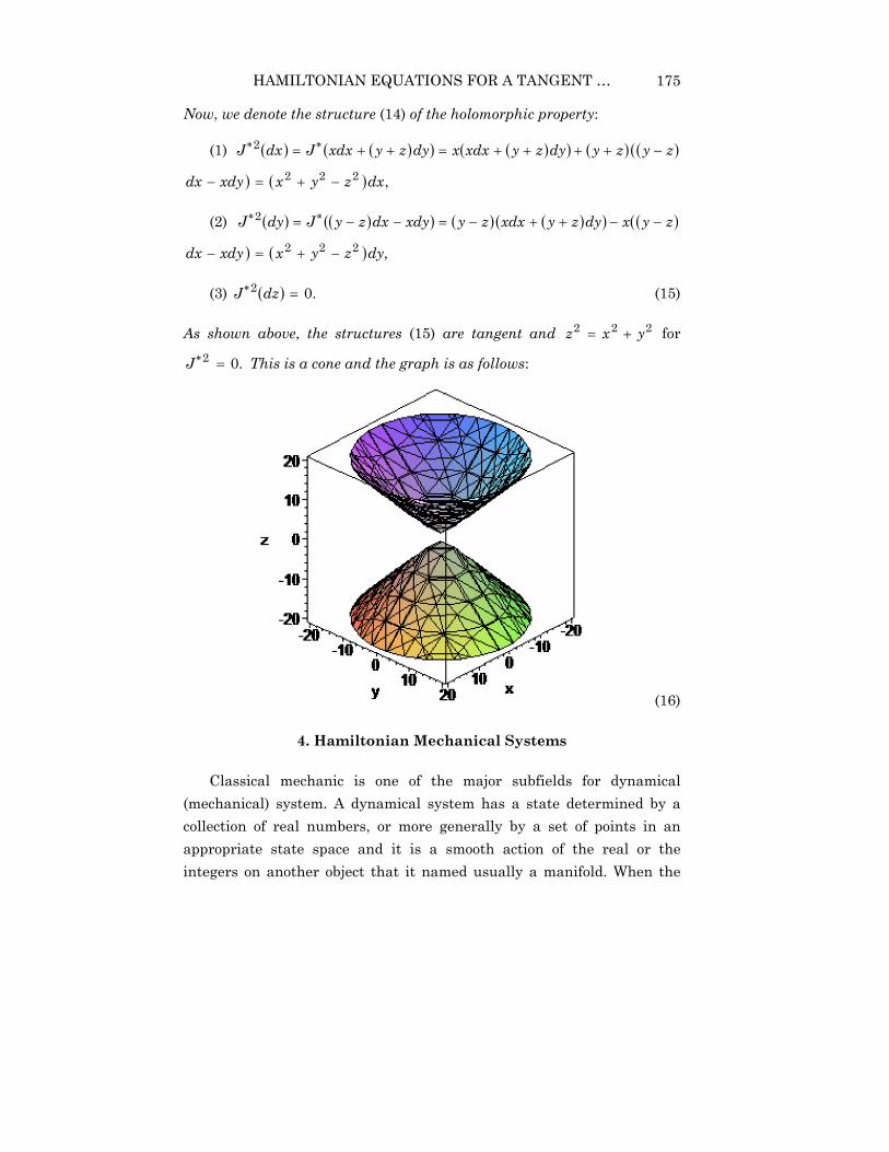
Now, we denote the structure (14) of the holomorphic property:
(1) ( ) ( )( ) ( )( ) ( ) (( )zyzydyzyxdxxdyzyxdxJdxJ −++++=++= ∗∗2
) ( ) ,222 dxzyxxdydx −+=−
(2) ( ) ( )( ) ( ) ( )( ) (( )zyxdyzyxdxzyxdydxzyJdyJ −−++−=−−= ∗∗2
) ( ) ,222 dyzyxxdydx −+=−
(3) ( ) .02 =∗ dzJ (15)
As shown above, the structures (15) are tangent and 222 yxz += for
.02 =∗J This is a cone and the graph is as follows:
(16)
4. Hamiltonian Mechanical Systems
Classical mechanic is one of the major subfields for dynamical (mechanical) system. A dynamical system has a state determined by a collection of real numbers, or more generally by a set of points in an appropriate state space and it is a smooth action of the real or the integers on another object that it named usually a manifold. When the

ZEKI KASAP 176
reals are acting, the mechanical system is called a continuous dynamical system, and when the integers are acting, the system is called a discrete dynamical system. At any given time, a dynamical system has a state given by a set of real numbers (a vector) that can be represented by a point in an appropriate state space. Dynamical systems theory is an area of mathematics used to describe the behaviour of complex dynamical systems, usually by employing differential equations or difference equations. The above-mentioned differential equations are found using the following ways:
Lemma 4. The closed 2-form on a vector field and 1-form reduction function on the phase space defined of a mechanical system is equal to the differential of the energy function 1-form of the Lagrangian and the Hamiltonian mechanical systems [17, 18].
Definition 11. Let M is the configuration manifold and its cotangent
manifold .MT ∗ By a symplectic form we mean a 2-form Φ on MT ∗ such that :
(i) Φ is closed, that is, ;0=Φd (ii) for each ∗∗∗ ×Φ∈ TMTMTz :,
R→M is weakly nondegenerate. If zΦ in (ii) is nondegenerate, we
speak of a strong symplectic form. If (ii) is dropped we refer to Φ as a
presymplectic form. Let ( )Φ∗ ,MT be a symplectic manifold. A vector
field MTMTXH∗∗ →: is called Hamiltonian if there is a 1C function
R→∗MTH : such that dynamical equation is determined by
.dHi HX =Φ (17)
We say that HX is locally Hamiltonian vector field if ΦHXi is closed and
where Φ shows the canonical symplectic form so that ( ),, ω=ΩΩ−=Φ ∗Jd ∗J a dual of ω,J a 1-form on .MT ∗ The trio ( )HXMT ,, Φ∗ is named
Hamiltonian system which it is defined on the cotangent bundle MT ∗ [19, 20].

HAMILTONIAN EQUATIONS FOR A TANGENT … 177
Definition 12. The vector field X on MT ∗ given by dHiX =ω is
called the geodesic flow of the metric g.
Definition 13. If ( ) MTba ∗→γ ,: is an integral curve of the
geodesic flow, then the curve ( )γp in M is called a geodesic.
The Hamiltonian of a system is defined to be the sum of the kinetic and potential energies expressed as a function of positions and their conjugate momenta. Recall from elementary physics that momentum of a particle, ,ip is defined in terms of its velocity iq by .iii qmp = In fact,
the more general definition of conjugate momentum, valid for any set of coordinates, is given in terms of the Lagrangian: ,ii qLp ∂∂=
.ii qLp ∂∂= Note that these two definitions are equivalent for
Cartesian variables. In terms of Cartesian momenta, the kinetic energy
is given by .221 ii
ni mpT ∑ =
= Then, the Hamiltonian, which is defined
to be the sum, ,VTH += expressed as a function of positions and
momenta, will be given by ( ) ( ),,,2, 12
1 niiniii qqVmppqH …+= ∑ =
where ,1pp = ., np… The function H is equal to the total energy of the
system. In terms of the Hamiltonian, the equations of motion of a system are given by Hamilton’s equations:
.,i
ii
i qHpp
Hq∂∂−=
∂∂= (18)
The solution of Hamilton’s equations of motion will yield a trajectory in terms of positions and momenta as functions of time. Hamilton’s equations can be easily shown to be equivalent to Newton’s equations and Hamilton’s equations can be used to determine the equations of motion of a system in any set of coordinates.

ZEKI KASAP 178
5. Hamilton Equations
Hamilton equations are an efficient use of classical mechanics to solve problems using mathematical modelling. In this part, we present, using (17), Hamilton equations for quantum and classical mechanics which are constructed on twistorial generalized Kähler manifolds. It is well-known that the quantum mechanical commutation relations for momentum and angular momentum give simple commutation relation for twistors and dual twistors (14). Hence the quantization rule for twistor theory: holomorphic structure of dual twistors (14) are represented for mechanical systems.
Proposition 2. Let ( )∗∗ JgMT ,, be on twistorial generalized Kähler
manifolds. Where in the calculations to be used (17). Imagine that the complex structures, a Liouville form and a 1-form on contact manifolds
are indicated by Ω∗,J and ,ω respectively. Think about a 1-form such
that
.dzxdyydx +−=ω (19)
Now, we obtain the Liouville form with (14) as follows:
( ) ( ) ( ) ( )dzJdyxJdxyJJ ∗∗∗∗ ++=ω=Ω
( ) ( ) .22 dyxzxyxdxxzxyx ++++−= (20)
It is well-known that if Φ is a closed on contact manifold ( ),,, ∗∗ JgMT
then Φ is also a symplectic structure on ( ).,, ∗∗ JgMT Therefore, the
2-form Φ shows the canonical symplectic form and derived from the 1-form Ω to find to mechanical equations. In this case the 2-form is calculated as:

HAMILTONIAN EQUATIONS FOR A TANGENT … 179
[( ) ( ) ]dyxzxyxdxxzxyxdyydxxd +−++−
∂∂+
∂∂=Ω−=Φ 22
( ) ( ) ( )
( ) ( ) ( )
∂++∂
+∂
+−∂+
∂++∂
+
∂+−∂
+∂
++∂+
∂+−∂
−=dydzz
xzxyxdxdzzxzxyxdydyy
xzxyx
dxdyyxzxyxdydxx
xzxyxdxdxxxzxyx
222
222
( ) .2 dzxdydzxdxdyxdxdxdyzyx ++−++= (21)
Proposition 3. Let HX be a vector field
,zZyYxXXH ∂∂+
∂∂+
∂∂= (22)
so that called to be Hamiltonian vector field associated with Hamiltonian energy H and determined by (17). Then there are
( ) ( )
∂∂−
∂∂−
∂∂−
∂∂++=Φ dxxdydyxdxxXdyxdxdxxdyXzyxXH 2
∂∂−
∂∂+
∂∂−
∂∂+ dyxdzdzxdyxXdxxdzdzxdxxX
( )
∂∂−
∂∂−
∂∂−
∂∂++− dxydydyydxxYdyydxdxydyYzyx2
∂∂−
∂∂+
∂∂−
∂∂+ dyydzdzydyxYdxydzdzydxxY
( )
∂∂−
∂∂−
∂∂−
∂∂++− dxzdydyzdxxZdyzdxdxzdyZzyx2
∂∂−
∂∂+
∂∂−
∂∂+ dyzdzdzzdyxZdxzdzdzzdxxZ
( ) ( )YdxzyxxXdzxXdyXdyzyx ++−+−++−= 22
.xZdyxZdxxYdzxYdx −−++ (23)
Furthermore, the differential of Hamiltonian energy H is obtained by
.dzzHdyy
HdxxHdH
∂∂+
∂∂+
∂∂= (24)

ZEKI KASAP 180
If these Equations (23) are solved for dHi HX =Φ
( ) ( ) zH
xyH
zyxxH
zyxX∂∂+
∂∂
++−
∂∂
++= 2
132
132
1
( ) ( ) zH
xyH
zyxxH
zyxY∂∂+
∂∂
+++
∂∂
++−= 2
132
132
1
( ) .2
321
21
2 zH
xzyx
yH
xxH
xZ∂∂++−
∂∂−
∂∂−= (25)
From here
( ) ( ) dxzH
xyH
zyxxH
zyxXH
∂∂+
∂∂
++−
∂∂
++= 2
132
132
1
( ) ( ) dyzH
xyH
zyxxH
zyx
∂∂+
∂∂
+++
∂∂
++−+ 2
132
132
1
( ) .2
321
21
2 dzzH
xzyx
yH
xxH
x
∂∂++−
∂∂−
∂∂−+ (26)
Consider the curve and its velocity vector ( ) txtMTI∂∂=α→⊂α ∗ ,: R
dztzdyt
ydx∂∂+
∂∂+ such that an integral curve of the Hamiltonian vector
field ,HX i.e., ( )( ) ( ) ., ItttXH ∈α=α Then we find the following
equations:
( ) ( ) ,21
321
321 dxt
xdxzH
xyH
zyxxH
zyx ∂∂=
∂∂+
∂∂
++−
∂∂
++
( ) ( ) ,21
321
321 dyt
ydyzH
xyH
zyxxH
zyx ∂∂=
∂∂+
∂∂
+++
∂∂
++−
( ) .2
321
21
2 dztzdzz
Hx
zyxyH
xxH
x ∂∂=
∂∂++−
∂∂−
∂∂− (27)
So, we find the following equations for motion:
HAMILTONIAN EQUATIONS FOR A TANGENT … 181
( ) ( ) ,21
321
321
zH
xyH
zyxxH
zyxtx
∂∂+
∂∂
++−
∂∂
++=
∂∂
( ) ( ) ,21
321
321
zH
xyH
zyxxH
zyxty
∂∂+
∂∂
+++
∂∂
++−=
∂∂
( ) .2
321
21
2 zH
xzyx
yH
xxH
xtz
∂∂++−
∂∂−
∂∂−=
∂∂ (28)
Therefore, the equations introduced in (28) are called Hamilton equations on twistorial generalized Kähler manifolds and then the triple
( )HXMT ,, Φ∗ is thought to be a Hamiltonian mechanical system
( )∗∗ JgMT ,, on twistorial generalized Kähler manifolds with space-
time points.
6. Equations Solving with Computer
The location of each object in space represented with maximum three dimensions in physical space. These three dimensions can be labelled by a combination of three chosen from the terms time, position, mass, length, width, height, depth, density, and breadth. In this study, (28) equations are partial differential equations on twistorial generalized Kähler manifolds such that its solved with Maple computation program. Implicit solution (28) for ( ) ( ) ( ) ( ) ( )ttzttyttx cos,sin, === is
( ) ( )( )xtFtzyxH ∗+∗−∗−= 61613,,, 1
( ) ( )( )xtFt ∗+∗−∗−∗∗ 616132cos 1
( ) ( ) ( )( )ytzxttFt ∗+∗∗−+∗−∗−∗∗ 313132sin 1
( ) ( ( ) ( ) )ytyxttFt ∗+∗∗−∗−+∗∗∗−∗ 313131313cos 1
( ) ( ) ( ) .2131321sin 1 xtzytFt ∗−∗∗−∗−∗+∗ (29)
As seen above (29) is a closed solution. To draw the graph of (29) must be made closed special preferences.

ZEKI KASAP 182
Example 2. Special values of (28);
( ) ( 21612341,,, PixPitzyxH ∗−∗−−∗=
( ) ) ( )212313141 ∗∗+∗∗−∗+ yPizx
( ( ) PixyPi ∗∗−∗−∗+∗∗− 31314148123 2
) ( ) ( ) .4,3143231 21 π=∗+∗−∗−∗∗+ tPiyzy
(30)
7. Discussion
A classical field theory explain the study of how one or more physical fields interact with matter which is used quantum and classical mechanics of physics branches. How the movement of objects in electrical, magnetically, and gravitational fields force is very important. Because, the classical theory of electromagnetism deals with electric and magnetic fields and their interaction with each other and with charges and currents. An electromagnetic field is a physical field produced by electrically charged objects and their locations over time.

HAMILTONIAN EQUATIONS FOR A TANGENT … 183
It is well-known that the motivation and one of the initial aims of twistor theory is to provide an adequate formalism for the union of quantum theory and general relativity. Twistor theory can also be used to solve non-linear differential equations, which are related to the self-
duality equations that describe instantaneous in .4R In this study, the Hamilton mechanical equations for space-time points (28) derived on twistorial generalized Kähler manifolds may be suggested to deal with problems in electrical, magnetically, and gravitational fields for the path of movement (30) of defined space moving objects [21, 22].
References
[1] R. Penrose, Twistor algebra, J. Math. Phys. 8 (1967), 345-366.
[2] R. Penrose, Twistor Theory, its Aims and Achievements, C. J. Isham, R. Penrose, D. W. Sciama (Eds.), Proceedings of Oxford Symposium on Quantum Gravity, Clarendon Press, Oxford, (1975), 268-407.
[3] R. Pantilie, On a class of twistorial maps, Differential Geometry and its Applications 26 (2008), 366-376.
[4] S. Ianus¸ S. Marchiafava, L. Ornea and R. Pantilie, Twistorial maps between quaternionic manifolds, arXiv:0801.4587v2, (2008).
[5] S. Cecotti, A. Neitzke and C. Vafa, Twistorial topological strings and a ∗tt geometry for N = 2 theories in 4d, arXiv:1412.4793v1, (2014).
[6] S. Santa-Cruz, Twistor geometry for hyper Kähler metrics on complex adjoint orbits, Annals of Global Analysis and Geometry 15 (1997), 361-377.
[7] R. Albuquerque, Twistorial constructions of special Riemannian manifolds.
[8] J. Davidov and O. Mushkarov, Twistor spaces of generalized complex structures, Journal of Geometry and Physics 56 (2006), 1623-1636.
[9] E. Loubeau and R. Pantilie, Harmonic morphisms between Weyl spaces and twistorial maps, Communications in Analysis and Geometry 14(5) (2006), 847-881.
[10] J. Davidov and O. Mushkarov, Twistorial construction of generalized Kähler manifolds, Journal of Geometry and Physics 57 (2007), 889-901.
[11] M. Dunajski, Twistor theory and differential equations, arXiv:0902.0274v2, (2009).
[12] S. Marchiafava, Twistorial maps between (para) quaternionic projective spaces, Bull. Math. Soc. Sci. Math. Roumanie Tome 52(100-3) (2009), 321-332.
[13] M. Tekkoyun, Mechanics systems on para-Kählerian manifolds of constant J-sectional curvature, http://arxiv.org/abs/0902.3569v1, (2009), 1-8.

ZEKI KASAP 184
[14] N. Nowaczyk, J. Niediek and M. Firsching, Basics of Complex Manifolds, (2009).
[15] W. Ballmann, Lectures on Kähler Manifolds, ESI Lectures in Mathematics and Physics, 2006.
[16] D. J. Griffiths, Introduction to Electrodynamics, Prentice Hall, ISBN 0-13-805326-X, 1999.
[17] J. Klein, Escapes variationnels et mécanique, Ann. Inst. Fourier, Grenoble 12 (1962).
[18] A. Ibord, The geometry of dynamics, Extracta Mathematicable 11(1) (1996), 80-105.
[19] M. de Leon and P. R. Rodrigues, Methods of Differential Geometry in Analytical Mechanics, Elsevier Sc. Pub., 1989.
[20] R. Abraham, J. E. Marsden and T. Ratiu, Manifolds Tensor Analysis and Applications, Springer, 2001.
[21] B. Thidé, Electromagnetic field theory, (2012).
[22] R. G. Martín, Electromagnetic Field Theory for Physicists and Engineers: Fundamentals and Applications, Granada, 2007.
g