twistor theory of higher-dimensional black holes

arX

iv:1

207.

0115

v1 [

gr-q

c] 3

0 Ju

n 20

12

Twistor Theory of

Higher-Dimensional Black Holes

Norman Metzner

Mathematical Institute St John’s CollegeUniversity of Oxford Oxford

Thesis submitted for the degree of

Doctor of Philosophy in Mathematics

Trinity Term 2012

http://arxiv.org/abs/1207.0115v1

iii

Acknowledgements

I would like to thank my supervisors Paul Tod and Lionel Masonfor the fruitful discussions and the guidance throughout all thestages towards this thesis. Furthermore, I am grateful to PiotrChruściel and Nicholas Woodhouse for sharing their thoughtson some ideas, to the German National Academic Foundation(Studienstiftung des deutschen Volkes), St John’s College Ox-ford and the Engineering and Physical Sciences Research Councilfor financial support, and to Mark Wilkinson, Parth Soneji andChristopher Hopper for making the days in the office so enjoy-able. Special mention to my wonderful wife Yulia backing me upand bearing with me at all times.

Abstract

The correspondence of stationary, axisymmetric, asymptotically flat space-timesand bundles over a reduced twistor space has been established in four dimensions.The main impediment for an application of this correspondence to examples inhigher dimensions is the lack of a higher-dimensional equivalent of the Ernst poten-tial. This thesis will propose such a generalized Ernst potential, point out wherethe rod structure of the space-time can be found in the twistor picture and therebyprovide a procedure for generating solutions to the Einstein field equations in higherdimensions from the rod structure, other asymptotic data, and the requirement ofa regular axis. Examples in five dimensions are studied and necessary tools aredeveloped, in particular rules for the transition between different adaptations of thepatching matrix and rules for the elimination of conical singularities.

v

Contents

Chapter 1. Introduction 1

Chapter 2. Mathematical Background 5

Chapter 3. Twistor Space 113.1. Definition of Twistor Space . . . . . . . . . . . . . . . . . . . . 113.2. Lines in PT . . . . . . . . . . . . . . . . . . . . . . . . . . . . 123.3. The Correspondence Space . . . . . . . . . . . . . . . . . . . . 123.4. Reality Structures . . . . . . . . . . . . . . . . . . . . . . . . . 13

Chapter 4. The Penrose-Ward Transform 154.1. Lax Pairs and Fundamental Solutions . . . . . . . . . . . . . . . 154.2. The Patching Matrix . . . . . . . . . . . . . . . . . . . . . . . 174.3. The Reverse Transform . . . . . . . . . . . . . . . . . . . . . . 174.4. The Abstract Form of the Transform . . . . . . . . . . . . . . . 18

Chapter 5. Yang’s Equation, σ-Model and Ernst Potential 215.1. Yang’s Equation and the J-Matrix . . . . . . . . . . . . . . . . 215.2. Reduction of Yang’s Equation . . . . . . . . . . . . . . . . . . . 225.3. Reduction of Einstein Equations . . . . . . . . . . . . . . . . . . 245.4. Solution Generation by the Symmetries of Yang’s Equation . . . . 28

Chapter 6. Black Holes and Rod Structure 296.1. Relevant Facts on Black Holes . . . . . . . . . . . . . . . . . . . 296.2. Rod Structure . . . . . . . . . . . . . . . . . . . . . . . . . . 32

Chapter 7. Bundles over Reduced Twistor Space 397.1. Reduced Twistor Space . . . . . . . . . . . . . . . . . . . . . . 397.2. The Twistor Construction . . . . . . . . . . . . . . . . . . . . . 427.3. Review of the Four-Dimensional Case . . . . . . . . . . . . . . . 46

Chapter 8. Twistor Approach in Five Dimensions 518.1. Bäcklund Transformations . . . . . . . . . . . . . . . . . . . . . 518.2. Higher-Dimensional Ernst Potential . . . . . . . . . . . . . . . . 538.3. Properties of P and the Bundle . . . . . . . . . . . . . . . . . . 608.4. Patching Matrix near the Axis and Twistor Data Integers . . . . . 61

Chapter 9. Patching Matrix for Relevant Examples 659.1. Five-Dimensional Minkowski Space . . . . . . . . . . . . . . . . 659.2. Twist Potentials on the Axis . . . . . . . . . . . . . . . . . . . 669.3. Asymptotic Minkowski Space-Times . . . . . . . . . . . . . . . . 689.4. Five-Dimensional Myers-Perry Solution . . . . . . . . . . . . . . 719.5. Black Ring Solutions . . . . . . . . . . . . . . . . . . . . . . . 77

vii

viii CONTENTS

Chapter 10. The Converse 8310.1. From Rod Structure to Patching Matrix — an Ansatz . . . . . . . 8410.2. Local Behaviour of J around a Nut . . . . . . . . . . . . . . . . 9410.3. Conicality and the Conformal Factor . . . . . . . . . . . . . . . 9610.4. Local Behaviour of P around a Nut: Switching . . . . . . . . . . 9810.5. Application to the Black Ring . . . . . . . . . . . . . . . . . . . 103

Chapter 11. Summary and Outlook 105

Appendix 107

Bibliography 117

CHAPTER 1

Introduction

Although initially proposed in four dimensions, the vacuum Einstein Field Equa-tions can be studied more generally in n dimensions. Higher-dimensional generalrelativity plays a role for example in string theory [40], the AdS/CFT correspon-dence, which relates the dynamics of an n-dimensional black hole with those ofquantum field theory in n−1 dimensions [32, 1], and scenarios involving large extradimensions and high-energy scattering are discussed in which higher-dimensionalblack holes might be produced in particle colliders [27]. Furthermore, black holespace-times are Ricci-flat Lorentzian manifolds and as such central objects of studyin differential geometry. This list of motivations was taken from [13, Sec. 1].

In four dimensions general relativity has led to various striking results aboutblack holes, for example concerning their horizon topology, their classification (seereferences in Section 6.1) or the laws of black hole mechanics [2]. Are these featuresexclusive to four-dimensional space-times or do some of them carry over to higherdimensions? Answers to these questions would provide valuable insights as wellas a better understanding of general relativity and its objects like black holes in abroader context [13, Sec. 1].

In four dimensions stationary and asymptotically-flat vacuum black holes canbe uniquely classified by their mass and angular momentum, and form a singlefamily, the Kerr solutions, see [6], references therein and Theorem 6.2. However, ageneralization of this statement to five dimensions, which would be a classficiationof five-dimensional, stationary, axisymmetric and asymptotically flat black holes bytheir mass and two angular momenta, does not hold as the space-times found byMyers & Perry [34] and Emparan & Reall [10] show. These examples of black holespace-times in five dimensions have topologically different horizons, so there cannotexist a continuous parameter to link them. Now the task is: Can we determine, orat least characterize, all stationary and asymptotically flat black hole solutions ofthe higher-dimensional vacuum Einstein field equations [13, Sec. 8]?

Since mass and angular momenta are not enough anymore to classify the solutions,an extra piece of information is needed. This extra piece was proposed to be theso-called rod structure [11, 21, 24] and Hollands & Yazadjiev [24] were able toshow that two stationary, axisymmetric and asymptotically flat black hole solutionswith connected horizon must be isometric, if their mass, angular momenta and rodstructures coincide. Thus the remaining problem is to prove that the only rodstructures giving rise to regular black hole solutions are those associated with theknown solutions or to find new examples.

Various strategies have been employed in order to address this question, amongwhich were direct approaches like the ones leading to the black ring, Bäcklundtransformations [33, Sec. 6.6] or other hidden symmetries [19]. Most often applied,however, was the method developed by Belinskiı & Zakharov [3], which uses the factthat the Einstein field equations for a stationary and axisymmetric space-time are

1

2 1. INTRODUCTION

integrable, see also [13, Sec. 5.2.2.2]. Via this ansatz they devised a purely algebraicprocedure for generating new solutions from known seeds that lead for example tothe discovery of a doubly-spinning black ring by Pomeransky & Sen’kov [37] and acandidate for a black hole with a Lens-space horizon [5].

In this thesis we are going to establish another way of constructing such solu-tions from the rod structure and other asymptotic data. The method is based ona twistor construction by which a holomorphic rank-(n − 2) vector bundle over aone-dimensional complex manifold is assigned to every stationary, axisymmetricsolution of the vacuum Einstein field equations in n dimensions. Under not veryrestrictive technical assumptions the bundle is fully characterized by only one tran-sition matrix, the so-called patching matrix, associated with each rod, and witha simple transformation from rod to rod. It was shown by Ward [46] that thecorrespondence can be better understood and made applicable for practical exam-ples with the help of a Bäcklund transformation. This was studied extensively in[49, 16, 17], but an application in more than four dimensions is not feasible withouta generalization of the Ernst potential.

As a first result we will therefore show that a modified version of a matrix alreadygiven in [31] satisfies the desired requirements.

Theorem 1.1. Let J be the matrix of inner products of Killing vectors for astationary and axisymmetric space-time in n dimensions. Then for any given rod(ai, ai+1) the matrix

J ′ =1

det A

1 −χt

−χ det A · A+ χχt

,

where A is adapted to (ai, ai+1) and χ is the vector of twist potentials for (ai, ai+1),is called higher-dimensional Ernst potential adapted to (ai, ai+1) and obtained fromJ by a Bäcklund transformation.

Following that, we quickly check that important results in four dimensions hold inthe same way in higher dimensions. Among these results is the important fact thatthe patching matrix is the analytic continuation of the Ernst potential J ′(0, z) =P (z).

As the second step we calculate the patching matrices P for the major exam-ples in five dimensions, which essentially requires the computation of various twistpotentials on the axis r = 0.

More importantly, the twistor correspondence provides a procedure for generatingsolutions from a given rod structure together with the asymptotic quantities, thatis based on the fact that P has simple poles at the nuts of the rod structure andthe known fall-off towards infinity. However, this ansatz contains numerous freeparameters and the aim is to fix these in terms of the given data by the use ofboundary conditions. For this it is inevitable to find out how the patching matriceswith adaptations to the different axis segments are related.

First this is done for the outer sections of the axis.

Theorem 1.2. Assume that we are given a rod structure with nuts at ai|ai ∈R1≤i≤N . If P+ is the patching matrix adapted to (aN ,∞), then P− = MP−1

+ M

with M =(

0 0 10 1 01 0 0

)is the patching matrix adapted to (−∞, a1).

With the help of this connection we are able to reconstruct the known space-timesflat space, Myers-Perry and the black ring from the rod structures with up to three

1. INTRODUCTION 3

nuts. However, we are not able to fix the conicality of the black ring, which needsfurther investigation of the behaviour of J , P and the conformal factor (appearingin the σ-model form of the metric) in a neighborhood of a nut. A definition of the(u, v)-coordinates can be found in Section 10.2.

Theorem 1.3. For a space-time regular on the axis the generic form of J in(u, v)-coordinates around a nut at u = v = 0, where two spacelike rods meet, is

J =

X0 u2Y0 v2Z0

· u2U0 u2v2V0

· · v2W0

, (1.1)

and, furthermore, one needs

• U0

v2e2ν= 1 as a function of v on u = 0,

• W0

u2e2ν= 1 as a function of u on v = 0.

If one of the rods is the horizon instead of a spacelike rod corresponding statementshold.

Building up on this, we obtain the following results about the conformal factor.

Proposition 1.4. On a segment of the axis where u = 0 we have U0

v2e2ν =

constant, and similarly where v = 0. Therefore, the factor(u2 + v2

)e2ν is con-

tinuous at the nut u = v = 0 and with the conventions leading to (1.1), the absenceof conical singularities requires

limv→0

U0 = limu→0

W0.

Last in the set of tools we show how P switches when going past a nut.

Theorem 1.5. Let at z = α be a nut where two spacelike rods meet and assumethat we have chosen a gauge where the twist potentials vanish when approaching thenut. Then

P− =

0 01

2(z − α)

0 1 0

2(z − α) 0 0

P+

0 0 2(z − α)

0 1 01

2(z − α)0 0

,

where P+ is adapted to u = 0 and P− is adapted to v = 0.

By this we can impose more boundary conditions on the free parameters in Pthat are possibly left and we have enough at hand to solve the conicality problemas exemplified for the black ring in Section 10.5.

This thesis is structured as follows. In Chapters 2, 3, 4, 5, 7 we give a detailed de-scription of the background material in order to make the thesis more self-contained,to familiarize the reader with the established construction and to identify the pointswhich impede a generalization to higher dimensions. The material for this purposeis mainly taken from [33, 17]. In Chapter 6 we revisit some relevant facts aboutblack holes. The aforementioned generalization of the Ernst potential follows inChapter 8, succeeded by the patching matrices for the examples in Chapter 9.Chapter 10 contains the reconstruction of P from the rod structure, results about

4 1. INTRODUCTION

the relation of different adaptations of P across nuts and the removal of conicalsingularities.

CHAPTER 2

Mathematical Background

This chapter is mainly based on Mason & Woodhouse [33, Ch. 2] and gives abrief summary of some mathematical tools which are needed later on. It is far fromexhaustive, and some parts are only aimed to make the reader familiar with thenotation used. In particular, we assume basic knowledge about principal bundlesand Yang-Mills theory as can be found for example in [29, 30].

The starting point for twistor theory is complex Minkowski space CM. For ourpurposes double null coordinates are often convenient, that is coordinates on CM inwhich the metric takes the form

ds2 = 2(dz dz − dw dw),

and the volume element is

ν = dw ∧ dw ∧ dz ∧ dz.

Then the vector fields ∂w, ∂w, ∂z , ∂z form a null tetrad at each point of CM. Ingeneral, a basis of 4-vectors W, W , Z, Z is called a null tetrad if

η(Z, Z) = −η(W, W ) = 1, 24 ν(W, W , Z, Z) = 1

where η is the metric tensor on CM, and all other inner products vanish.Within this setting we can recover various real spaces (“real slices”) by imposing

reality conditions on w, w, z, z.

• Euclidean real slice E: We identify real Cartesian coordinates x0, x1, x2,x3 with w, w, z, z via

(z ww z

)=

1√2

(x0 + ix1 −x2 + ix3

x2 + ix3 x0 − ix1

).

That is, we get E by imposing the reality conditions w = −w and z = z.• Minkowski real slice M: The real coordinates x0, x1, x2, x3 on M are

identified with w, w, z, z via

(z ww z

)=

1√2

(x0 + x1 x2 − ix3

x2 + ix3 x0 − x1

),

that is we pick out the real space by the condition that z and z should bereal, and that w = w.

For the definition of self-duality and anti-self-duality we need the Hodge staroperation. To clarify notation and conventions first a short reminder. Let (M, g)be an n-dimensional Riemannian or pseudo-Riemannian manifold. Given a p-formβ on M with (skew-symmetric) components βab...c its exterior derivative dβ has

5

6 2. MATHEMATICAL BACKGROUND

components ∂[aβbc...d] where the square brackets stand for antisymmetrization.1

The exterior or wedge product β ∧ γ with a q-form γ has components

β[ab...cγde...f ].

Now let ε be the n-dimensional alternating symbol, that is ε[a...b] = εa...b and

ε0...n = 1, and ∆ =√

| det(gab)|. We then define the (Hodge) dual of β to be the(n− p)-form ∗β with components

∗ βab...c =1

(n− p)!∆ε de...f

ab...c βde...f , (2.1)

where indices are raised and lowered with the metric gab or its inverse gab. Tosee that the definition is actually independent of the basis consider p vector fieldsX1, . . . , Xp with their covariant images θ1, . . . , θp (according to the metric) and fixa volume form d vol. Then ∗β is defined as the unique (n− p)-form satisfying

β(X1, . . . , Xp) dvol = (∗β) ∧ θ1 ∧ . . . ∧ θp.

This is a basis independent definition of ∗β and coincides with (2.1), since in coor-dinates

dvol = ∆εa...d.

Thus one can think of ∗β as the complement of β with respect to the volume form(and the appropriate prefactor). For example in terms of an oriented orthonormalbasis e1, . . . , en (of a vector space) the Hodge star operation is defined completelyby

∗(ei1 ∧ . . . ∧ eik ) = eik+1∧ . . . ∧ ein ,

where i1, . . . , ik, ik+1, . . . , in is an even permutation of 1, . . . , n. Of particularinterest for us are 2-forms on (CM, η) where we have

∗βab =1

2∆εabcdη

ceηdfβef .

Using the properties of the alternating symbol, it follows that the Hodge star oper-ation is idempotent, that is ∗2 = 1, thus has eigenvalues ±1.2

Definition 2.1. A 2-form is called self-dual (SD) if ∗β = β, and anti-self-dual(ASD) if ∗β = −β.

The space of 2-forms then decomposes into the direct sum of eigenspaces, becausein double null coordinates we have

α = dw ∧ dz, α = dw ∧ dz, ω = dw ∧ dw − dz ∧ dz (2.2)

as a basis for SD 2-forms, and

dw ∧ dz, dw ∧ dz, dw ∧ dw + dz ∧ dz

as a basis for ASD 2-forms.

1For a(

0p

)tensor

T[ab...c] =1

p!

∑

σ∈Sp

sgn(σ)Tσ(a)σ(b)...σ(c)

where Sp is the group of permutations of p elements. The symmetrization T(ab...c) is defined inthe same way but without the signum.2In general, on a Riemannian manifold (M,g) for a p-form β it is ∗∗β = (−1)p(n−p)sβ, where s isthe signature of g. For complex manifolds the concept of signature is void, thus we can set s = 1and then ∗2 = id for 2-forms on a four-dimensional manifold.

2. MATHEMATICAL BACKGROUND 7

Let E be a rank-n vector bundle with a connection D, that is a differentialoperator that maps sections s of E to 1-forms with values in E and in a localtrivialization it is given by

Ds = ds+ Φs

where Φ is matrix-valued 1-form called gauge potential, potential or sometimes alsoconnection. In a general gauge theory, that is a principal bundle P (M,G) over a(pseudo-) Riemannian manifold M with with gauge groupG ⊆ GL(n), the curvatureof D is the matrix-valued 2-form F = Fab dxa ∧ dxb with

Fab = ∂aΦb − ∂bΦa + [Φa,Φb].

The Yang-Mills equations are

DF = 0, D ∗ F = 0

where the first one is called the Bianchi identity and the second one is theEuler-Lagrange equation of the Lagrangian density 1

2 tr(F ∧ ∗F ) = 14 tr(FabF

ab).We then see that if F is SD or ASD then D ∗ F = ±DF = 0, that is the second setof Yang-Mills equations follow from the Bianchi identity.

Important objects for twistor theory is null 2-planes.

Definition 2.2. Let Π be an affine 2-plane in CM and Π⊥ the normal bundle ofΠ. The 2-plane Π is called (partially) null if 0 ( TΠp ∩ Π⊥

p ( TΠp for all p ∈ Π,

and it is called (totally) null if TΠ ∩ Π⊥ = TΠ.

Hence, totally null means that η(A,B) = 0 for all tangent vectors A, B of Π.From now on when we speak about null 2-planes we will always mean totally null2-planes (unless mentioned differently). With each null 2-plane Π we associate atangent bivector π = A∧B where A, B are independent tangent vectors of Π. Thetangent bivector has components πab = A[aBb].

Lemma 2.3. If Π is a null 2-plane, then πabπab = 0, and πab dxa ∧ dxb is either

SD or ASD.

Proof. First of all we observe that π is determined up to scale by the tangentspace of Π, because another choice of independent tangent vectors can be written asa linear combination of A and B and thus gives the same π up to a nonzero scalarfactor. Conversely, the tangent space of Π is given by all P b with πabP

b = 0, sinceA, B are null and orthogonal. But π can also be characterized up to a nonzeroscalar factor by the condition that ∗πabP b = 0 for all P b tangent vectors of Π. Thisfollows from πab = A[aBb], and ∗πab = εabcdA

cBd which implies that ∗πabP b = 0 ifand only if P is a linear combination of A and B. Hence, π = µ ∗ π for some µ , 0.However, the eigenvalues of ∗ are ±1, therefore πab = ∗πab or πab = − ∗ πab, thatis π SD or ASD. Again from πab = A[aBb] and the fact that A, and B are null and

orthogonal it is obvious that πabπab = 0.

Definition 2.4. An affine null 2-plane Π is called an α-plane if π is SD and aβ-plane if π is ASD.

In double null coordinates the surfaces of constant w, z and w, z, respectively,have tangent bivectors dw∧dz and dw∧dz, respectively, and are therefore α-planes.

If π is the tangent bivector of an α-plane through the origin, then it must bea linear combination of the 2-forms in (2.2). It is only determined up to a scalar

8 2. MATHEMATICAL BACKGROUND

factor, that is we can set the coefficient of dw ∧ dz to 1 without loss of generality.Then we have

π = dw ∧ dz − ζ(dw ∧ dw − dz ∧ dz) + µ dw ∧ dz.

So, the nonzero coefficients are πwz = 1, πww = −πzz = −ζ and πwz = µ. Then therequirement from Lemma 2.3 turns into

0 = πabπab = πabπcdη

acηbd = −µ− ζ2 − ζ2 − µ ⇔ µ = −ζ2.

This implies

πab = L[aM b]

where

L = ∂w − ζ∂z , M = ∂z − ζ∂w

for some ζ ∈ C. The case where the coefficient of dw ∧ dz vanishes yields ζ = 0, sothat π = dw ∧ dz (up to a constant) and L = ∂w, M = ∂z. There is no point inthe argument where we needed that our null tetrad is induced by coordinates, thatis the above statement is also true if we set L = W − ζZ and M = Z − ζW forsome null tetrad W , W , Z, Z not necessarily induced by coordinates. Conversely,L and M span an α-plane through the origin for every ζ ∈ C. Including the pointζ = ∞ by mapping it to the α-plane spanned by ∂w and ∂z then yields a one-to-onecorrespondence between α-planes through the origin and points of the Riemannsphere, Πζ ↔ ζ. This correspondence will be important for the characterization oftwistor spaces.

As a last point in this chapter a reminder about equivalence and reconstruction ofholomorphic vector bundles (these statements can be found in standard textbookssuch as [20, 18]). Let π : E → X be a rank-r holomorphic vector bundle withan open cover (Ui)i∈I of X and trivialization functions (biholomorphic maps) hi :π−1(Ui) → Ui × Cr.

The (holomorphic) transition functions gij : Ui ∩ Uj → GL(r,C) for all i, j ∈ Iare obtained from the biholomorphic maps

gij ≔ hi h−1j : Ui ∩ Uj × Cr → Ui ∩ Uj × Cr,

which are of the form gij(x, v) = (x, gij(x)v). By construction the transition func-tions obviously satisfy the relations

gijgjk = gik, gii = id . (2.3)

Two holomorphic vector bundles E → X and F → X are called isomorphic ifthere exists a bijective map f : E → F such that f and its inverse are vector bundlehomorphisms, that is f is a fibre-preserving holomorphic map πE = πF f suchthat for any x ∈ X a linear map fx : Ex → Fx is induced and analogously for thef−1.

Given two systems of transition functions, (gij)i,j∈I and (gi′j′)i′,j′∈I with covers(Ui)i∈I and (Vi′ )i′∈I′ , then they are called equivalent if for a common refinement ofthe open covers (Wk)k∈K there are holomorphic maps fk : Wk → GL(r,C) with

fkgkl = gklfl.

The transition functions with respect to the refined cover can be taken as the re-strictions of the initial transition functions and a common refinement is for exampleobtained by taking all possible intersections of Ui and Vi′ .

2. MATHEMATICAL BACKGROUND 9

Proposition 2.5. For holomorphic vector bundles the following statements hold.

(1) Let Uii∈I be an open covering of X, and let gij ∈ GLr(OX(Ui ∩ Uj))satisfy the cocycle relation (2.3). Then there exists as holomorphic vectorbundle E of rank r with these transition functions. [20]

(2) Isomorphic bundles can be represented by equivalent systems of transitionfunctions. [18]

CHAPTER 3

Twistor Space

In this chapter the twistor space for complexified Minkowski space is introducedusing Mason & Woodhouse [33, Sec. 9.2].

3.1. Definition of Twistor Space

In the previous chapter we have seen that α-planes through the origin in CM arespanned by L = ∂w − ζ∂z and M = ∂z − ζ∂w or by ∂w and ∂z in the limitingcase (ζ = ∞). As before, the coordinates w, z, w, z will always be double-nullcoordinates. Thus, a general α-plane, not necessarily passing through the origin,is labelled by three complex coordinates: the parameter ζ which determines thetangent space, together with the parameters

λ = ζw + z and µ = ζz + w (3.1)

that are constant over the α-plane.

Definition 3.1. The twistor space of CM is the three-dimensional complex man-ifold consisting of all (affine) α-planes in CM.

A way to determine the global geometry is by writing the equations of an α-planein homogeneous form

zZ2 + wZ3 = Z0, wZ2 + zZ3 = Z1 (3.2)

with complex constants Zα, α = 0, 1, 2, 3. The order of these constants is a conven-tion in twistor theory. If Z2

, 0, then (3.2) is equivalent to (3.1) for

λ =Z0

Z2, µ =

Z1

Z2, ζ =

Z3

Z2.

In the case Z2 = 0, Z3, 0, the parameter ζ must be infinite and the tangent space

is spanned by ∂w and ∂z. Consequently, we can identify the twistor space of CMwith an open subset of CP3 if we include this α-plane of constant w, z and regardthe Zαs as homogeneous coordinates.

The excluded points of CP3 are

I = [Z0 : Z1 : Z2 : Z3

]∈ CP3 : Z2 = Z3 = 0

.

There are 2 homogeneous coordinates left which parameterize I, hence it is a CP1

and the twistor space of CM is, as a complex manifold, CP3 − CP1. We can coverthe twistor space of CM by two coordinate patches V and V with V being thecomplement of the plane Z2 = 0 (that is the plane ζ = ∞) and V being thecomplement of the plane Z3 = 0 (that is the plane ζ = 0). The parameters λ, µ, ζare coordinates on V , and on V we can use coordinates λ, µ, ζ with

λ =Z0

Z3, µ =

Z1

Z3, ζ =

Z2

Z3,

11

12 3. TWISTOR SPACE

which on the overlap V ∩ V gives the relations

λ =λ

ζ, µ =

µ

ζ, ζ =

1

ζ.

For the twistor space we denote by T the copy of C4 on which (Z0, Z1, Z2, Z3) arelinear coordinates, and by PT the corresponding projective space CP3.

Now let U ⊂ CM and assume that its intersection with each α-plane is connected(but possibly empty).1

Definition 3.2. The twistor space of U is the subset

P = Z ∈ PT : Z ∩ U , ∅of PT.

If U is open, then P is open, and if U = CM, then P is the complement of I.

Remark 3.3.

(1) For many aspects of twistor theory it turns out that spinor calculus is asuitable tool. However, in our context we do not gain anything by usingspinors and thus they are not going to be introduced in this work.

(2) The Klein correspondence shows that compactified CM together withthe complex conformal group can be identified with a CP3 ⊂ CP5, theKlein quadric, together with the so-called projective general linear groupGL(4,C)/C×. [33, Sec. 2.4 and 9.2]

3.2. Lines in PT

The equations (3.2) allow further conclusions: if we hold w, z, w, z fixed, andvary Zα, then the equations determine a two-dimensional subspace of T, that is aprojective line in PT. This is the Riemann sphere of α-planes through the point inCM with coordinates w, z, w, z which we denote by x. It corresponds to the twistorspace of x ⊂ CM.

Two points x, y ∈ CM are null separated if and only if they lie on an α-plane,hence if and only if x∩ y , ∅. In other words, two lines in the twistor space intersectif and only if the corresponding points are separated by a null vector. A conformalmetric (that is a class of conformally equivalent metrics) is completely determinedby saying when two vectors are null separated (Appendix A). Hence, the conformalgeometry of CM is encoded in the linear geometry of PT.

3.3. The Correspondence Space

Let U be a subset of CM. The correspondence space F is the set of pairs (x, Z)with x ∈ U and Z an α-plane through x. It is fibred over U and P by projections

Fq

⑦⑦⑦⑦⑦⑦ p

U P

1The connectivity assumption is not necessary for the considerations in this chapter, but will latermake the Penrose-Ward transform work in a natural way.

3.4. REALITY STRUCTURES 13

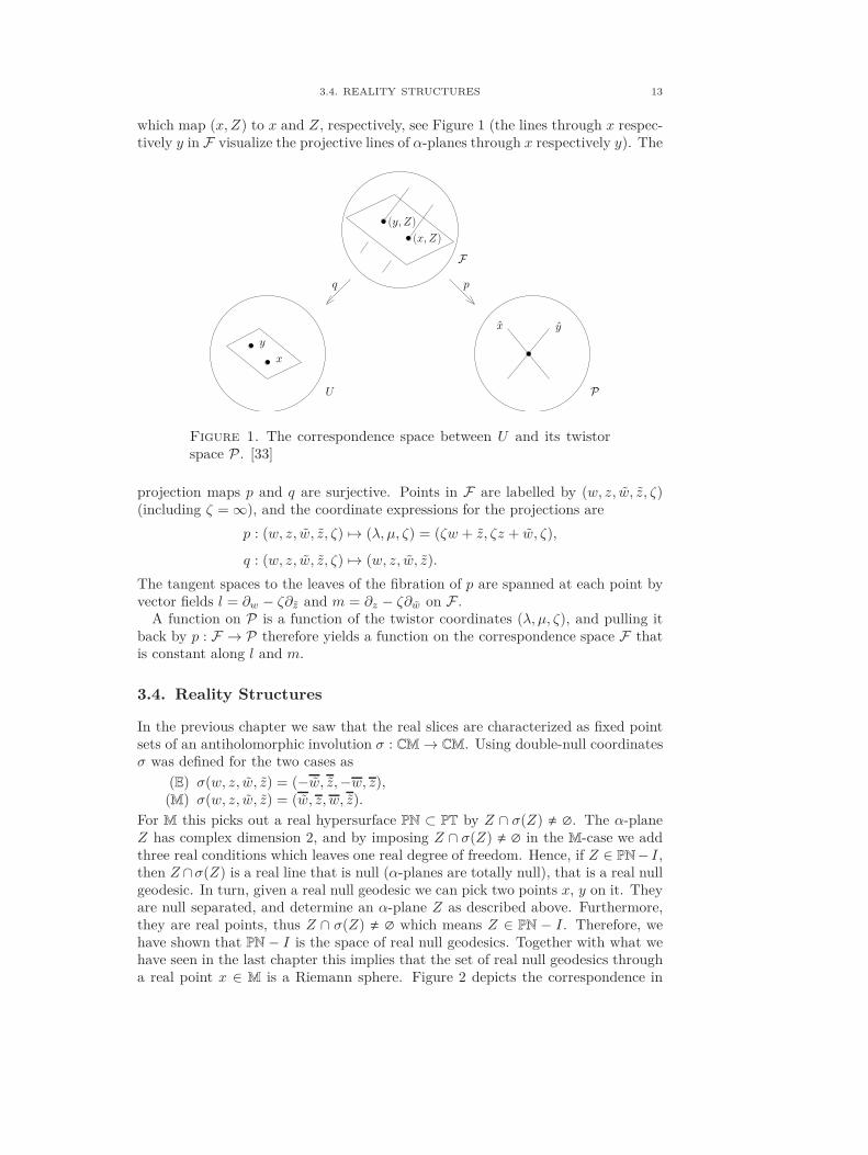
which map (x, Z) to x and Z, respectively, see Figure 1 (the lines through x respec-tively y in F visualize the projective lines of α-planes through x respectively y). The

y

x y

P

p

F

(y, Z)

(x, Z)

q

U

x

Figure 1. The correspondence space between U and its twistorspace P . [33]

projection maps p and q are surjective. Points in F are labelled by (w, z, w, z, ζ)(including ζ = ∞), and the coordinate expressions for the projections are

p : (w, z, w, z, ζ) 7→ (λ, µ, ζ) = (ζw + z, ζz + w, ζ),

q : (w, z, w, z, ζ) 7→ (w, z, w, z).

The tangent spaces to the leaves of the fibration of p are spanned at each point byvector fields l = ∂w − ζ∂z and m = ∂z − ζ∂w on F .

A function on P is a function of the twistor coordinates (λ, µ, ζ), and pulling itback by p : F → P therefore yields a function on the correspondence space F thatis constant along l and m.

3.4. Reality Structures

In the previous chapter we saw that the real slices are characterized as fixed pointsets of an antiholomorphic involution σ : CM→ CM. Using double-null coordinatesσ was defined for the two cases as

(E) σ(w, z, w, z) = (−w, z,−w, z),(M) σ(w, z, w, z) = (w, z, w, z).

For M this picks out a real hypersurface PN ⊂ PT by Z ∩ σ(Z) , ∅. The α-planeZ has complex dimension 2, and by imposing Z ∩ σ(Z) , ∅ in the M-case we addthree real conditions which leaves one real degree of freedom. Hence, if Z ∈ PN− I,then Z ∩σ(Z) is a real line that is null (α-planes are totally null), that is a real nullgeodesic. In turn, given a real null geodesic we can pick two points x, y on it. Theyare null separated, and determine an α-plane Z as described above. Furthermore,they are real points, thus Z ∩ σ(Z) , ∅ which means Z ∈ PN − I. Therefore, wehave shown that PN− I is the space of real null geodesics. Together with what wehave seen in the last chapter this implies that the set of real null geodesics througha real point x ∈ M is a Riemann sphere. Figure 2 depicts the correspondence in

14 3. TWISTOR SPACE

this real case. It also indicates how a point in PN− I corresponds to a locus in M

x

Z

x

Riemann sphere

M

twistor picture PN− I

Z

light ray

Figure 2. The correspondence between M and PN− I. [36]

and a point x ∈ M represented by its light cone corresponds to a locus (Riemannsphere) in PN − I. Thus, the relationship between U and its twistor space P is anon-local correspondence in general.

CHAPTER 4

The Penrose-Ward Transform

This chapter is about the Penrose-Ward transform which associates a solutionto the anti-self-dual Yang-Mills (ASDYM) equation on a domain U in CM to aholomorphic vector bundle on the twistor space P of U , using Mason & Woodhouse[33, Sec. 10.1 and 10.2].

That raises the question: What is the special importance of the ASDYM equa-tion for our considerations? To answer this, we have to say a few words aboutintegrable systems. In classical mechanics the notion of integrability is a preciseconcept. However, for systems obeying partial differential equations in which thereare infinitely many degrees of freedom, we do not have a clear-cut characterizationof integrability. A lot of theories were developed and it is easy to give examples of‘integrability’, yet there is no single effective characterization that covers all cases[33, Ch. 1].

But whatever the definition of integrability is, a reduction of an integrable system,which is obtained by imposing a symmetry or specifying certain parameters, alwaysyields another integrable system. Thus we have a partial ordering, in the sense thatwe say system A is less than system B if A is a reduction of B. This orderingmotivates the search for a ‘maximal element’, that is an integrable system fromwhich all others can be derived. Such a system has not yet been found, but it turnsout that almost all known systems in dimension 1 and 2, and a lot of importantsystems in dimension 3 arise as reductions of the ASDYM equation [33, Ch. 4.1].

The example of special significance for us will be the Ernst equation for stationaryaxisymmetric gravitational fields.

4.1. Lax Pairs and Fundamental Solutions

Let D be a connection on a complex rank-n vector bundle E over some region U inCM, and F its curvature 2-form. If D = d + Φ, then F = Fab dxa ∧ dxb, where in acoordinate induced local trivialization

Fab = ∂aΦb − ∂bΦa + [Φa,Φb].

The ASD conditions then take in double-null coordinates the form

Fzw = ∂zΦw − ∂wΦz + [Φz ,Φw] = 0,

Fzw = ∂zΦw − ∂wΦz + [Φz ,Φw] = 0,

Fzz − Fww = ∂zΦz − ∂zΦz − ∂wΦw + ∂wΦw

+ [Φz,Φz] − [Φw,Φw] = 0.

(4.1)

With

Dw = ∂w + Φw, Dz = ∂z + Φz, Dw = ∂w + Φw, Dz = ∂z + Φz

15

16 4. THE PENROSE-WARD TRANSFORM

the ASD condition can be written as

[Dz ,Dw] = 0, [Dz ,Dw] = 0, [Dz ,Dz ] − [Dw ,Dw] = 0, (4.2)

so that the ASDYM equation corresponds to the vanishing of the curvature on everyα-plane. Equivalently, we can require that the Lax pair of operators

L = Dw − ζDz , M = Dz − ζDw

should commute for every value of the complex ‘spectral parameter’ ζ, where L andM act on vector-valued functions on CM.

This last compatibility condition says that for a section s of E, represented by acolumn vector of length n, the linear system

Ls = 0, Ms = 0

can be integrated for each fixed value of ζ. Therefore, putting n independent solu-tions together, we obtain an n × n matrix fundamental solution f (dependent onζ) such that the columns of f form a frame field for E consisting of sections thatare covariantly constant on the α-planes tangent to ∂w − ζ∂z and ∂z − ζ∂w. Hence-forth, we suppose that U is open and that each α-plane that meets U intersects itin a connected and simply connected set, for example U an open ball. The secondcondition about simply connectedness ensures that the sections are single valued.

The matrix f satisfies

(∂w + Φw)f − ζ(∂z + Φz)f = 0,

(∂z + Φz)f − ζ(∂w + Φw)f = 0,(4.3)

and depends holomorphically on ζ (varied over the complex plane), and the coor-dinates w, z, w, z. However, if f were regular, by which we mean holomorphicwith non-vanishing determinant, on the entire ζ-Riemann sphere, then Liouville’stheorem would imply that f is independent of ζ. Consequently,

Dwf = Dzf = Dwf = Dzf = 0,

in other words f were covariantly constant and the connection flat.Given a choice of gauge, f is unique up to f 7→ fH where H is a non-singular

matrix-valued function of ζ, w, z, w, z such that

∂wH − ζ∂zH = 0, ∂zH − ζ∂wH = 0. (4.4)

So, H is essentially a function of λ = ζw + z, µ = ζz + w and ζ.If P denotes the twistor space of U , and V , V is a two-set Stein open cover of P1

such that V is contained in the complement of ζ = ∞, and V is contained in thecomplement of ζ = 0, then f can be regarded as a function on the correspondencespace F and H as the pull-back of a holomorphic function on V , as by (4.4) H isconstant along the leaves of p : F → P .

If D is not flat, f cannot be chosen so that it is regular for all finite values of ζand at ζ = ∞. However, with ζ = 1

ζwe get a solution f for the linear system

ζDwf − Dz f = 0, ζDz f − Dwf = 0, (4.5)

which is holomorphic on the whole ζ-Riemann sphere except for ζ = 0. This solutionis unique up to f 7→ f H, where H is holomorphic on V and satisfies the equationcorresponding to (4.4).

1For Stein manifolds see for example Field [15, Def. 4.2.7] and how the two-set cover can be chosensee for example Popov [38, Sec. 3.3].

4.3. THE REVERSE TRANSFORM 17

4.2. The Patching Matrix

On the overlap of the domains of f and f in F we must have

f = fP,

where P satisfies (4.4), and thus it is the pull-back by p of a holomorphic functionon V ∩ V . We call P patching matrix associated to D. It is determined by D upto equivalence P ∼ H−1PH where H is regular on V , H is regular on V and bothsatisfy (4.4). The matrices in the equivalence class of P are called patching data ofD. If P is in the equivalence class of the identity solution, then P = H−1H , hence

fH = f H. (4.6)

The left-hand side of (4.6) is regular in V , and the right-hand side is regular in V ,so we have a global solution in ζ, and therefore vanishing curvature. If there is nosuch solutions, the curvature has to be nonzero.

The transformation of Φ under a gauge transformation is

Φ 7→ Φ′ = g−1Φg + g−1 dg,

where g is a function of w, z, w, z with values in the gauge group. A solution forthe new potential can be attained by replacing f 7→ g−1f and f 7→ g−1f , whichleaves the patching matrix unchanged.

We have obtained a map which assigns patching data to every ASDYM field. Itis called forward Penrose-Ward transform. Indeed, the converse is true as well, thatis a patching matrix encodes an ASDYM field.

4.3. The Reverse Transform

For the following arguments we need the so-called Birkhoff’s factorization theorem.We do not state it in full precision, but only to the extend that is necessary here(for more details see Mason & Woodhouse [33, Sec. 9.3]).

Suppose P (λ, µ, ζ) is holomorphic matrix-valued function on V ∩ V with non-vanishing determinant. Birkhoff’s factorization theorem says that for fixed valuesof w, z, w, z we can factorize P in the form

P (ζw + z, ζz + w, ζ) = f−1∆f,

where f(w, z, w, z, ζ) is regular for |ζ| ≤ 1, f(w, z, w, z, ζ) is regular for |ζ| ≥ 1(including ζ = ∞), and ∆ = diag(ζk1 , . . . , ζkn) for some integers k1, . . . , kn whichmay depend on the point in CM. For functions P for which ∆ = 1, this factorizationis unique up to f 7→ cf , f 7→ cf for some constant c ∈ GL(n,C). Furthermore,given a P such that ∆ = 1 at some point of CM, then ∆ = 1 in an open set of CM.2

Given a Birkhoff factorization for fixed (w, z, w, z) such that

P (ζw + z, ζz + w, ζ) = f−1f,

2This statement is consequence of Birkhoff’s factorization theorem. If P (w, ζ) depends smoothlyon additional parameters w = (w1, w2, . . . ) and ∆ = 1 at some point w, then ∆ = 1 in an open

neighbourhood of w, and f , f can be chosen such that they depend smoothly on the parameters.The statement also holds if we replace ‘smooth’ by ‘holomorphic’ in the case that P dependsholomorphically on ζ (in a neighbourhood of the unit circle) and on the complex parameters w.Attempts to extend the factorization to the entire parameter space typically fail on a submanifoldof codimension 1, where ∆ ‘jumps’ to another value than the identity [33, Prop. 9.3.4].

18 4. THE PENROSE-WARD TRANSFORM

we can recover Φ in terms of f or f by

Φw − ζΦz = (−∂wf + ζ∂zf)f−1 = (−∂wf + ζ∂z f)f−1 (4.7)

with a similar equation for the other two components. By the uniqueness statementany other factorization is given by f ′ = gf , f ′ = gf , where g is independent of ζ.The new potential Φ′, which is obtained from f ′, f ′, is related to the previous onevia

Φ = g−1Φ′g + g−1 dg.

This is obvious regarding (4.7). Hence, P determines Φ up to gauge transformations.It remains to show that our patching matrix P is the same as the one that is

associated to the ASDYM field we have just constructed. In other words, we mustensure that applying first the reverse and then the forward Penrose-Ward transformto the function P gets us back to the starting point.

Suppose P is chosen such that ∆ = 1 at some point of CM, then ∆ = 1 in anopen set U of CM. The constancy of P along ∂w − ζ∂z implies

0 = (∂w − ζ∂z)(f−1f) = −f−1((∂w − ζ∂z)f)f−1f + f−1(∂w − ζ∂z)f,

or equivalently(∂wf − ζ∂zf)f−1 = (∂wf − ζ∂z f)f−1, (4.8)

at every point in U and for all ζ in some neighbourhood of the unit circle. The left-hand side of (4.8) is holomorphic for |ζ| < 1, and the right-hand side is holomorphicfor |ζ| > 1 except for a simple pole at infinity. Therefore, by an extension ofLiouville’s theorem both sides have to be of the form −Φw + ζΦz , where Φw andΦz are independent of ζ. We take them to be the two components of Φ. Thesame procedure with ∂z − ζ∂w instead of ∂w − ζ∂z defines Φz and Φw. Then, byconstruction

Dwf − ζDzf = 0, Dz − ζDwf = 0,

where D = d + Φ acts on the columns of f . Thus, the linear system associated toD is integrable, and D = d + Φ is ASD.

The above constructions gives an explicit formula of the potential Φ using f andf .

Lemma 4.1. The gauge potential Φ is given in terms of f and f by

Φ = h∂h−1 + h∂h−1,

where h = f |ζ=0 and h = f∣∣ζ=∞.

Proof. Setting ζ = 0 in (4.3) gives the first two components Φw, Φz; setting

ζ = 0 in (4.5) gives the second pair of components Φw, Φz.

So, we have shown that D can be recovered from the patching matrix, and indeedeven more, namely that any patching matrix such that ∆ = 1 at some point of CMgenerates a solution of the ASDYM equation in an open set of CM.

4.4. The Abstract Form of the Transform

The construction as described so far is very explicit and suggests that it dependson the cover V , V and the chosen coordinates. However, it does not show, as statedin its abstract form, that the transform is in fact between ASDYM fields on U andholomorphic vector bundles on P . The above choices were only a way to representthe bundle in a concrete way.

4.4. THE ABSTRACT FORM OF THE TRANSFORM 19

If D is an ASD connection on a rank-n vector bundle B → U , then the patchingmatrix P on U determines a rank-n vector bundle B′ → P , where P can be regardedas the transition matrix between the holomorphic trivializations (of B′) over V andV . The fibre of B′ attached to a point Z ∈ P is

B′Z = s ∈ Γ(Z ∩ U,B) : Ds|Z∩U = 0,

where Γ(Z ∩ U,B) is the space of sections of B over Z ∩ U . That is the fibreover an α-plane Z ∈ P is the vector space of covariantly constant sections of Bover Z ∩ U with respect to D. Because P has the Birkhoff factorization with∆ = 1 at each point of U , the restriction of B′ to each line in P correspondingto a point in U is holomorphically trivial. The holomorphic bundle is uniquelydetermined up to equivalence by D, as the freedom in the construction of P from D isprecisely the freedom in choice of two local holomorphic trivializations. Conversely,given B′ → P , the patching matrix P (and hence D) can be recovered in a directgeometrical way.

Theorem 4.2 (Ward [47]). Let U ⊂ CM be an open set such that the intersectionof U with every α-plane that meets U is connected and simply connected. Thenthere is a one-to-one correspondence between solutions to the ASDYM equation onU with gauge group GL(n,C) and holomorphic vector bundles B′ → P such thatB′|x is trivial for every x ∈ U .

Proof. See Mason & Woodhouse [33, Thm. 10.2.1].

CHAPTER 5

Yang’s Equation, σ-Model and Ernst Potential

We will see how the ASDYM can be written in a form called Yang’s equationusing Mason & Woodhouse [33, Sec. 3.3]. Then it is shown how Yang’s equationturns by a symmetry reduction into the Ernst equation which describes stationaryaxisymmetric solutions to the Einstein equations [33, Sec. 6.6].

5.1. Yang’s Equation and the J-Matrix

The ASD condition on the curvature 2-form ∗F = −F is coordinate-independentand invariant under gauge transformations as well as under conformal isometries ofCM. It can be written in other forms that are more tractable for certain aspects,even though some of the symmetries are broken.

The first two equations of (4.1), equivalent to

[Dz ,Dw] = 0, [Dz ,Dw] = 0,

are an integrability condition for the existence of matrix-valued functions h and hon CM such that

∂wh+ Φwh = 0, ∂zh+ Φzh = 0,

∂wh+ Φwh = 0, ∂z h+ Φzh = 0.

The potential Φ determines h and h uniquely up to h 7→ hB, h 7→ hA, whereB and A are matrices depending only on w, z and w, z, respectively. For a gaugetransformed potential Φ 7→ gΦg−1+g−1 dg we can replace h 7→ g−1h and h 7→ g−1h,which leaves the expression h−1h invariant.

We define Yang’s matrix [50] as J ≔ h−1h. It is determined by the connectionD up to J 7→ A−1JB. Note that h and h satisfy the same differential equationsas those in Lemma 4.1. Thus, the definition for Yang’s matrix is equivalent toJ = f(ζ = 0)f−1(ζ = ∞) with f and f as in Chapter 4. To consider the conversedirection let J = h−1h be a Yang’s matrix. The connection D is determined by J ,since we have

J−1∂J = J−1∂wJ dw + J−1∂zJ dz

= h−1h ∂w(h−1h) dw + w ↔ z

=(h−1h(∂wh

−1)h+ h−1∂wh)

dw + w ↔ z

=(−h−1(∂wh)h−1h+ h−1∂wh

)dw + w ↔ z

=(h−1Φwh+ h−1∂wh

)dw + w ↔ z,

(5.1)

21

22 5. YANG’S EQUATION

so that Φ is equivalent to J−1∂J by the gauge transformation Φ 7→ hΦh−1+h−1 dh.1

Given the matrix J we see that the first two equations of (4.1) are implied by (5.1),because

Φw = 0, Φz = 0, Φw = J−1∂wJ, Φz = J−1∂zJ

yields the first equation in (4.1) trivially, and the second one follows from

∂zΦw−∂wΦz + [Φz ,Φw]

= ∂z(J−1∂wJ) − ∂w(J−1∂zJ) + [J−1∂zJ, J

−1∂wJ ]

= 0.

A calculation similar to (5.1) shows that

∂w(J−1∂wJ) − ∂z(J−1∂zJ) = h−1(Fww − Fzz)h,

which is equivalent to Fww −Fzz under the above gauge transformation, and hencethe ASD equations are equivalent to Yang’s equation

∂w(J−1∂wJ) − ∂z(J−1∂zJ) = 0. (5.2)

However, they are no longer covariant under conformal transformations as thiswould change the 2-planes spanned by ∂w, ∂z and ∂w, ∂z .

Geometrically the construction of J can be interpreted as follows. Starting fromthe original gauge we make a transformation by g = h or g = h, respectively. Thisyields an equivalent gauge with vanishing Φw, Φz in the first case and vanishingΦw, Φz in the second case. If we have frame fields e1, . . . , en and e1, . . . , en,respectively, corresponding to the new gauge potentials, then

Dwei = 0, Dzei = 0, (5.3)

Dw ei = 0, Dz ei = 0, (5.4)

for i = 1, . . . , n. Furthermore, by definition of Yang’s matrix ej = eiJij . Therefore,J is the linear transformation from a frame field satisfying (5.3) to a frame fieldsatisfying (5.4). The connection potentials in the frames ei and ei are, respectively,

J−1∂J and J∂J−1.

The freedom in the construction of J from D is the freedom to transform the firstframe by B and the second frame by A.

5.2. Reduction of Yang’s Equation

In this section we show how Yang’s equation can be reduced by an additionalsymmetry so that it provides the linkage to Einstein equations.

Such a reduction can in general be approached as follows. Suppose we are givena two-dimensional subgroup of the conformal group, generated by two conformalKilling vectors X and Y , which span the tangent space of the orbit of our two-dimensional symmetry group at each point. To impose the symmetry on a solutionof the ASDYM equation, we require that the Lie derivative of the gauge potential Φalong X and Y vanishes.2 If the symmetry group is Abelian, [X,Y ] = 0, then there

1Note that after the gauge transformation the potential hΦh−1 + h−1 dh has vanishing w and zcomponent.2This requirement can be justified in a more systematic way if invariant connections, Lie derivateson sections of vector bundles etc. are introduced [33]. Here the Lie derivative of Φ along theKilling fields is the ordinary Lie derivative operator on differential form.

5.2. REDUCTION OF YANG’S EQUATION 23

exists a coordinate system with X , Y as the first two coordinate vector fields and bythe symmetry the components of Φ depend only upon the second pair of coordinates.The reduced version of equation (4.1) is obtained by changing the coordinates anddiscarding the derivatives with respect to the ignorable coordinates.

Another way is to impose the symmetry on Yang’s equation which is not alwaysstraightforward and we will see how it works in our case.

We are interested in the reduction by the commuting Killing vectors

X = w∂w − w∂w, Y = ∂z + ∂z.

The coordinates can be adapted by the transformation

w = reiθ, w = re−iθ, z = t− x, z = t+ x.

Then the metric is easily calculated to have the form

ds2 = dt2 − dx2 − dr2 − r2 dθ2,

and the Killing vectors are X = −2i∂θ, Y = 2∂t so that the symmetries are arotation θ 7→ θ + θ0 and a time translation t 7→ t+ t0.

In the Minkowski real slice the coordinates are real and the spatial metric isof cylindrical polar form. Thus, a reduction by X and Y refers to stationary ax-isymmetric solutions of the ASDYM equation and their continuations to CM. Thecrucial point for our considerations is the coincidence that apart from their rolein Yang-Mills theory the reduced equation turns out to be equivalent to the Ernstequation for stationary axisymmetric gravitational fields in general relativity.

We want to construct Yang’s matrix for the invariant potential in this stationaryaxisymmetric reduction. First, we note that it is still possible to choose the invariantgauge such that Φw = Φz = 0 and

Φ = −P dw

w+Q dz, (5.5)

where3 P and Q depend only on x and r. This can be seen as follows. Above wehave shown that for h being a solution of

∂wh+ Φwh = 0, ∂zh+ Φzh = 0, (5.6)

the gauge transformation with g = h yields a potential with Φw = Φz = 0, because(5.6) is equivalent to

h−1Φwh+ h−1∂wh = 0, h−1Φzh+ h−1∂zh = 0.

The integrability of (5.6) and hence the existence of h was ensured by the ASDcondition (4.2).

Now with the additional symmetry the question arises whether this is still possiblebut with h and Φ depending on x and r only. Under a gauge transformation wethen have

Φw 7→ h−1Φwh+1

2e−iθh−1hr, Φz 7→ h−1Φzh− 1

2h−1hx,

which is obtained by just substituting the coordinates and discarding the depen-dency on t and θ. In the same way the first equation of (4.1) becomes

− 1

2∂xΦw − 1

2e−iθ∂rΦz + [Φz,Φw] =

[Φz − 1

2∂x,Φw +

1

2e−iθ∂r

]= 0. (5.7)

3This P should not be confused with the Patching matrix.


Then, analogous to the general case, (4.1) in form of (5.7) is exactly the integrabilitycondition for the existence of an invariant gauge in which Φw = Φz = 0 and whereΦ and h depend only on x and r, that is

Φwh+1

2e−iθ∂rh = 0, Φzh− 1

2∂xh = 0.

Using the notation from (5.5) and by a similar calculation like above the secondequation in (4.1), Fzw = 0, takes the form

Px + rQr + 2[Q,P ] = 0, (5.8)

and the third equation, Fzz − Fww = 0, becomes

0 = ∂zΦz − ∂wΦw = −1

2∂xQ+

1

2e−iθ∂r

(P

w

),

or equivalently

Pr − rQx = 0. (5.9)

Condition (5.8) guarantees the existence of Yang’s matrix J(x, r) such that

Φw = −P

w= J−1∂wJ =

1

2eiθJ−1∂rJ, Φz = J−1∂zJ,

equivalent to

2P = −rJ−1∂rJ, 2Q = J−1∂xJ. (5.10)

It can again be interpreted as a change of gauge, but this time h and h depend onlyon x and r, hence so does J .

Starting with a matrix J(x, r), and defining the gauge potential by (5.10), it isan easy calculation that (5.8) is satisfied. Equation (5.9) becomes

r∂x(J−1∂xJ) + ∂r(rJ−1∂rJ) = 0. (5.11)

So, every solution to (5.11) determines a stationary axisymmetric ASDYM fieldand every stationary axisymmetric ASDYM field can be obtained in that way. TheYang’s matrix J determines the connection up to J 7→ A−1JB with constant ma-trices A and B. Note that in the general case above A, B depended on w, z andw, z, respectively. But here we restricted to gauge transformations such that thecondition Φw = Φz = 0 is preserved, hence they have to be constant (formula forgauge transformation of Φ involves derivatives of h, respectively h).

5.3. Reduction of Einstein Equations

The next step will be to show how reduced Yang’s equation (5.11) emanates froma reduction of the Einstein equations. This was originally discovered by Witten[48], Ward [46].

Let gab be a metric tensor in n dimensions (real or complex), and Xai , i =

0, . . . , n− s− 1, be n− s commuting Killing vectors that generate an orthogonallytransitive isometry group with non-null (n− s)-dimensional orbits. This means thedistribution of s-plane elements orthogonal to the orbits of Xi is integrable, in otherwords [U, V ] is orthogonal to all Xi whenever U and V are orthogonal to all Xi.

Define J = (Jij) ≔ (gabXai X

bj ), and denote by ∇ the Levi-Civita connection. We

have

XkJij = (LXkg)(Xi, Xj) + g(LXk

Xi, Xj) + g(Xi,LXkXj) = 0,

5.3. REDUCTION OF EINSTEIN EQUATIONS 25

as the first term vanishes due to the fact that Xk is a Killing vector, and the lasttwo terms since the Killing vectors commute. Thus J is constant along the orbitsof the Killing vectors. The Killing equation is

0 = LXigab = ∇aXib + ∇bXia, (5.12)

and since

[Xi, Xj] = 0 ∀ i, j (5.13)

we get

∂bJij = ∇b(Xai Xja) = Xa

i ∇bXja +Xaj ∇bXia

(5.12)= Xa

i ∇bXja −Xaj ∇aXib

(5.13)= Xa

i ∇bXja −Xai ∇aXjb

(5.12)= 2Xa

i ∇bXja.

(5.14)

This yields

Xaj ∇aXib = Xa

i ∇aXjb = −Xai ∇bXja = −1

2∂bJij .

Let U and V be vector fields orthogonal to the orbits. From

0 = ∇a(Ua V bXib︸︷︷︸=0

) − ∇a(V a U bXib︸︷︷︸=0

)

= (∇aUa)V bXib︸︷︷︸

=0

+Ua(∇aVb)Xib + UaV b(∇aXib) − U ↔ V

we obtain

UaV b∇aXib − V aU b∇aXib = −XibUa∇aV

b +XibVa∇aU

b

= −Xib(Ua∇aV

b − V a∇aUb)

= −Xib[U, V ]b

= 0,

where the last step follows from the orthogonal transitivity. This result togetherwith the Killing equation ∇aXib = ∇[aX|i|b] leads to

UaV b∇aXib = U [aV b]∇aXib = 0,

UaXbj∇aXib =

1

2Ua∂aJij ,

XajX

bk∇aXib =

1

2Xaj ∂aJki = 0.

However,1

2Jjk(

(∂aJki)Xjb − (∂bJki)Xja

),

where J ijJjk = δik,4 gives the same expressions when contracted with combinations

of Killing and orthogonal vectors. Hence, they must have the same components,

∇aXib =1

2Jjk(

(∂aJki)Xjb − (∂bJki)Xja

). (5.15)

Moreover, for a Killing vector X we can use the Ricci identity

∇b∇cXd = RabcdXa

4Here we need that the orbits of the isometry group are non-null, otherwise J would be degenerate.


with Rabcd the Riemann tensor, to take the second derivative of (5.15). After somecomputations (see Appendix C), we get

RabXai X

bj = −1

2Jik

√g−1∂a(

√ggabJkl∂bJlj),

where g = det(gab) and Rab = Rcacb is the Ricci tensor. If the Einstein vacuumequations, Rab = 0, hold, then

∂a(√ggabJkl∂bJlj) = 0. (5.16)

Since J is constant along the orbits (5.16) is essentially an equation on S, whereS is the quotient space by the Killing vectors identified with any of the s-surfacesorthogonal to the orbits. Denote by hab the metric on S and by D the correspondingLevi-Civita connection so that we get for the determinant

g = det gab = −r2 det(hab),

where −r2 = detJ .5 We know that for functions u on S covariant and partialderivative are equal ∂au = Dau. Considered this together with the expression forthe Laplace-Beltrami operator

D2u = DaDau =

1√|h|∂a

(√|h|hab∂bu

)

equation (5.16) becomesDa(rJ

−1DaJ) = 0, (5.17)

where the indices now run over 1, . . . , s and are lowered and raised with hab and itsinverse. Now remembering that

d detJ = detJ tr(J−1 dJ) ⇒ d(log detJ) = tr(J−1 dJ)

we can take the trace of (5.17) to get furthermore

0 = Da(r tr(J−1DaJ)) = Da(rDa(log detJ))

= Da(rDa(log −r2)) = Da(2r · 1

rDar)

= 2D2r,

hence r is harmonic on S. From now on we assume that the gradient of r is notnull.

In the case s = 2 isothermal coordinates always exist (see Appendix D), that iswe can write the metric on S in the form

e2ν(dr2 + dx2)

where x is the harmonic conjugate to r.6 As the Killing vectors commute, thereexist coordinates (y0, . . . , yn−3), where the Xi are the first n− 2 coordinate vectorfields. Taking furthermore the isothermal coordinates for the last two components,the full the metric then has the form

ds2 =n−3∑

i,j=0

Jij dyidyj + e2ν(dr2 + dx2), (5.18)

5The sign might vary depending on the signature of the metric and the Killing vectors (spacelikeor timelike). In some of the literature the condition is r2 = | det J |. Here it is adapted to theLorentzian case with one timelike and one spacelike Killing vector.6The function x is said to be harmonic conjugate to r, if x and r satisfy the Cauchy-Riemannequations.

5.3. REDUCTION OF EINSTEIN EQUATIONS 27

which is known as the (Einstein) σ-model. In this case (5.17) reduces to (5.11) andwe obtain the following proposition.

Proposition 5.1 (Proposition 6.6.1 in Mason & Woodhouse [33]). Let gab bea solution to Einstein’s vacuum equation in n dimensions. Suppose that it admitsn− 2 independent commuting Killing vectors generating an orthogonally transitiveisometry group with non-null orbits, and that the gradient of r is non-null. ThenJ(x, r) is the Yang’s matrix of a stationary axisymmetric solution to the ASDYMequation with gauge group GL(n− 2,C).

The partial converse of the Proposition yields a technique for solving Einstein’svacuum equations as follows. Any real solution J(x, r) to reduced Yang’s equa-tion (5.11) such that

(a) detJ = −r2,(b) J is symmetric

determines a solution to the Einstein vacuum equations, because we can reconstructthe metric from given J and e2ν via (5.18), and then (5.11) is equivalent to thevanishing of the components of Rab along the Killing vectors (as we have shownabove). The remaining components of the vacuum equations can be written as

2i∂ξ(log(re2ν

))= r tr

(∂ξ(J−1

)∂ξJ

), (5.19)

with ξ = x + ir, together with the complex conjugate equation (if x and r arereal), where ξ is replaced by ξ = x − ir and i by −i. These equations can beobtained by a direct calculation of the Christoffel symbols, curvature tensors and soon [21, App. D, Eq. (D9)]. They are automatically integrable if (5.11) is satisfiedand under the constraint detJ = −r2 (see Appendix E), and they determine eν

up to a multiplicative constant. The constraint, however, is not significant for thefollowing reason. We know that in polar coordinates u = log r is a solution to the(axisymmetric) Laplace equation

∂r(r∂ru) + r∂2xu = 0, (5.20)

so is u = c log r+ log d for constants c and d. Now suppose J is a solution to (5.11),and consider euJ = drcJ . Plugging this new matrix in (5.11), we see that it is againa solution of reduced Yang’s equation if (5.20) holds. The determinant constraintcan thus be satisfied by an appropriate choice of the constants, since we have

det(euJ) = e(n−2)u detJ = dn−2r(n−2)c detJ.

The condition J = J t is a further Z2 symmetry of the ASD connection.This coincidence between Einstein equations and Yang’s equation is remarkable,

since, although we started from a curved-space problem, by the correspondence itcan essentially be regarded as a problem on Minkowski space reduced by a timetranslation and a rotation, hence on flat space.

Considering the case n− 2 = s = 2, Yang’s matrix J can be written as

J =

(fα2 − r2f−1 −fα

−fα f

), (5.21)

where f and α are functions of x and r. It can be read off that the metric takes theform

ds2 = f(dt− α dθ)2 − f−1r2 dθ2 − e2ν(dr2 + dx2).

If f and α are real for real x and r this is known as the stationary axisymmetricgravitational field written in canonical Weyl coordinates.


5.4. Solution Generation by the Symmetries of Yang’s Equation

A tedious but straightforward calculation shows that in canonical Weyl coordinatesreduced Yang’s equation (5.11) becomes

r2∇2 log f + (f∂rα)2 + (f∂xα)2 = 0,

∂r(r−1f2∂rα) + ∂x(r−1f2∂xα) = 0,

(5.22)

where ∇2 = r−1∂r(r∂r) + ∂2x for real r is the axisymmetric form of the three-

dimensional Laplacian in cylindrical polar coordinates. The second equation is anintegrability condition for ψ with

∂xψ = −r−1f2∂rα, ∂rψ = −r−1f2∂xα,

or equivalentlyr∂xψ + f2∂rα = 0, r∂rψ − f2∂xα = 0.

If we consider the matrix

J ′ =1

f

(ψ2 + f2 ψ

ψ 1

)(5.23)

instead of J ,7 we find that (5.11) for J ′ again comes down to (5.22), but with αreplaced by ψ as one of the variables. Solutions to Einstein’s vacuum equationscan now be obtained by solving (5.11) for J ′ subject to the conditions detJ ′ = 1,J ′ = J ′t. In this context (5.11) is called Ernst equation and the complex functionE = f + iψ is the Ernst potential [14], which is often taken as the basic variable inthe analysis of stationary axisymmetric fields. We will also refer to J ′ as the Ernstpotential.

Note that (5.11) has the obvious symmetry J 7→ AtJA, where A ∈ SL(2,C) isconstant.8 This corresponds to the linear transformation

(X Y ) 7→ (X Y )A (5.24)

of Killing vectors in the original space-time. Yet, the construction of J ′ is notcovariant with respect to general linear transformations in the space of Killingvectors, that is for (5.24) we do not have J ′ 7→ AtJ ′A. Given a solution of theEinstein vacuum equations in form of J ′, this leads to a method of generating newsolutions. First, recover the corresponding J by solving for α in terms of ψ and f .Then replace J by CtJC, C ∈ SL(2,C), and construct J ′ from the new J . Againreplace J ′ by DtJ ′D, D ∈ SL(2,C), and so on. This produces an infinite-parameterfamily of solutions to the Einstein vacuum equations starting from one originalseed (if C and D are real, the transformations preserve the reality, stationarity andaxisymmetry of the solutions as well).

7Since ψ is only determined up to constant J ′ is only determined up to

J ′ 7→

(1 0γ 1

)J ′

(1 γ0 1

)

for a constant γ.8The requirement detA = 1 is necessary to preserve the constraint det J ′ = 1.

CHAPTER 6

Black Holes and Rod Structure

A remarkable consequence of Einstein’s theory of gravitation is that under certaincircumstances an astronomical object cannot exist in an equilibrium state and hencemust undergo a gravitational collapse. The result is a space-time in which there isa “region of no escape” — a black hole. Black hole space-times are of interest notonly in four but also in higher dimensions.

This chapter will provide basic knowledge in general relativity that is neededlater on. Yet, proofs or further details are omitted at many points as this would bebeyond the scope of our discussion. Moreover, we will see what questions arise inhigher-dimensional black hole space-times and in the next chapter we will describehow twistor theory can be useful in tackling these problems.

In the following a space-time will be a real time-orientable and space-orientable1

Lorentzian manifold, where not stated differently.

6.1. Relevant Facts on Black Holes

The following definitions are taken from Wald [45] and Chruściel & Costa [6, Sec. 2].Denote by J ±(m) the causal future or past of a space-time point m. An importantconcept is asymptotic flatness which roughly speaking means that the gravitationalfield and matter fields (if present) become negligible in magnitude at large dis-tance from the origin. More precisely we say an n-dimensional space-time (M, g)is asymptotically flat and stationary if M contains a spacelike hypersurface Sext

diffeomorphic to Rn−1\B(R), where B(R) is an open coordinate ball of radius R,that is contained in a hypersurface satisfying the requirements of the positive en-ergy theorem and with the following properties. There exists a complete Killingvector field ξ which is timelike on Sext (stationarity) and there exists a constantα > 0 such that, in local coordinates on Sext obtained from Rn−1\B(R), the metricγ induced by g on Sext, and the extrinsic curvature tensor Kij of Sext, satisfy thefall-off conditions

γij − δij = Ok(r−α), Kij = Ok−1(r−1−α)

for some k > 1, where we write f = Ok(rα) if f satisfies

∂k1· · ·∂kl

f = O(rα−l), 0 ≤ l ≤ k.

In [6, Sec. 2.1] it is argued that these assumptions together with the vacuum fieldequations imply that the full metric asymptotes that of Minkowski space.

The Killing vector ξ models a “time translation symmetry”. The one-parametergroup of diffeomorphisms generated by ξ is denoted by φt : M → M . Let Mext =

1In fact, one can argue that time-orientability implies space-orientability [23, Sec. 6.1].

29

30 6. BLACK HOLES AND ROD STRUCTURE

⋃t φt(Sext) be the exterior region, then the domain of outer communications is

defined as

〈〈Mext〉〉 = J +(Mext) ∩ J −(Mext).

We call B = M\J −(Mext) the black hole region and its boundary H+ = ∂B theblack hole event horizon.2 Analogously, the white hole and the white hole eventhorizon are W = M\J +(Mext) and H− = ∂W . So, if the space time containsa black hole, that means it is not (entirely) contained in the causal past of itsexterior region. H = H+ ∪ H− is a null hypersurface generated by (inextendible)null geodesics [23, p. 312].

The second type of symmetry we will impose models a rotational symmetry. Wesay a space-time admits an axisymmetry if there exists a complete spacelike Killingvector field with periodic orbits. This is a U(1)-symmetry so we imagine it as a rota-tion around a codimension-2 hypersurface. As shown in Myers & Perry [34, Sec. 3.1]and Emparan & Reall [13, Sec. 1.1], note that for dimM > 4 there is the possibilityto rotate around multiple independent planes (if M is asymptotically flat). Forspatial dimension n− 1 we can group the coordinates in pairs (x1, x2), (x3, x4), . . .where each pair defines a plane for which polar coordinates (r1, ϕ1), (r2, ϕ2), . . . canbe chosen. Thus there are N = ⌊n−1

2 ⌋ independent (commuting) rotations each as-sociated to an angular momentum. An n-dimensional space-time M will be calledstationary and axisymmetric if it admits n − 3 of the above U(1) axisymmetriesin addition to the timelike symmetry. However, note that this yields an importantlimitation. For globally asymptotically flat space-times we have by definition anasymptotic factor of Sn−2 in the spatial geometry, and Sn−2 has isometry groupO(n− 1). The orthogonal group O(n− 1) in turn has Cartan subgroup U(1)N withN = ⌊n−1

2 ⌋, that is there cannot be more than N commuting rotations. But eachof our rotational symmetries must asymptotically approach an element of O(n− 1)so that U(1)n−3 ⊆ U(1)N , and hence

n− 3 ≤ N =

⌊n− 1

2

⌋,

which is only possible for n = 4, 5. Therefore, stationary and axisymmetric solutionsin our sense can only have a globally asymptotically flat end in dimension four andfive. However, much of the theory, for example the considerations in Chapter 5, isapplicable in any dimension greater than four so that henceforth we still considerstationary and axisymmetric space-times and it will be explicitly mentioned if extracare is necessary.

Note for example that we have to change the above definitions of a black hole andstationarity in dimensions greater or equal than 6 because they require asymptoticalflatness. Instead of asking Sext to be diffeomorphic to Rn\B(R) we set the conditionthat Sext is diffeomorphic to Rn\B(R)×N , where B(R) is again an open coordinateball of radius R and N is a compact manifold with the relevant dimension. Thisis also called asymptotic Kaluza-Klein behaviour. The fall-off conditions then haveto hold for the product metric on Rn\B(R) × N . The definition of stationarity isverbatim the same only with other asymptotic behaviour of Sext.

The time translation isometry must leave the event horizon of the black holeregion invariant as it is completely determined by the metric which is invariantunder the action of ξ. Hence ξ must lie tangent to the horizon, but a tangent vectorto a hypersurface with null normal vector must be null or spacelike. So, ξ must be

2This definition does in fact not depend on the choice of Sext [6, Sec. 2.2].

6.1. RELEVANT FACTS ON BLACK HOLES 31

null or spacelike everywhere on the horizon. This motivates the following definition.A null hypersurface N is called a Killing horizon of a Killing vector ξ if (on N ) ξ isnormal to N , that is ξ is in particular null on N . The integral curves of the normalvector of a null hypersurface are in fact geodesics and these geodesics generate thenull hypersurface.3 If l is normal to N such that ∇ll = 0 (affinely parameterized),then ξ = f · l and

∇ξξ = f∇l(fl) = ξ(f) · l + f2∇ll = f−1ξ(f) · ξ = κ · ξ,where κ = ξ(ln |f |) is the so-called surface gravity. It can be shown that

κ2 = −1

2(∇µξν)(∇µξν)|N ,

and that κ is constant on the horizon. Thus, the following definition makes sense: AKilling horizon is called non-degenerate if κ , 0, and degenerate otherwise. Hence-forth, we will restrict our attention to non-degenerate horizons, since it is a nec-essary assumption in the upcoming theorems and degenerate horizons may have asomewhat pathological behaviour.

The following theorem links the two notions of event and Killing horizon.

Theorem 6.1 (Theorem 1 in Hollands et al. [25]). Let (M, gab) be an analytic,asymptotically flat n-dimensional solution of the vacuum Einstein equations con-taining a black hole and possessing a Killing field ξ with complete orbits which aretimelike near infinity. Assume that a connected component, H, of the event horizonof the black hole is analytic and is topologically R × Σ, with Σ compact, and thatκ , 0. Then there exists a Killing field K, defined in a region that covers H and theentire domain of outer communication, such that K is normal to the horizon andK commutes with ξ.

This theorem essentially states that the event horizon of a black hole that hassettled down is a Killing horizon (not necessarily for ∂t). In four dimensions thistheorem has already been proven earlier [23]. In four dimensions Theorem 6.1 is anessential tool in the proof of the following uniqueness theorem, which is the resultof a string of papers [26, 4, 22, 39].

Theorem 6.2. Let (M, g) be a non-degenerate, connected, analytic, asymptot-ically flat, stationary and axisymmetric four-dimensional space-time that is non-singular on and outside an event horizon, then (M, g) is a member of the two-parameter Kerr family. The parameters are mass M and angular momentum L.

Since stationarity can be interpreted as having reached an equilibrium, this saysthat in four dimensions the final state of a gravitational collapse leading to a blackhole is uniquely determined by its mass and angular momentum. The assumptionof axisymmetry is actually not necessary in four dimensions, as it follows from thehigher-dimensional rigidity theorem.

Theorem 6.3. Let (M, gab) be an analytic, asymptotically flat n-dimensionalsolution of the vacuum Einstein equations containing a black hole and possessing aKilling field ξ with complete orbits which are timelike near infinity. Assume that aconnected component, H, of the event horizon of the black hole is analytic and istopologically R× Σ, with Σ compact, and that κ , 0.

3This and some of the following statements can be found in standard textbooks or lecture notes,for example [44].


(1) If ξ is tangent to the null generators of H, then the space-time must bestatic; in this case it is actually unique (for n = 4 the Schwarzschildsolution). [41]

(2) If ξ is not tangent to the null generators of H, then there exist N , N ≥ 1,additional linear independent Killing vectors that commute mutually andwith ξ. These Killing vector fields generate periodic commuting flows, andthere exists a linear combination

K = ξ + Ω1X1 + . . .+ ΩNXN , Ωi ∈ R,so that the Killing field K is tangent and normal to the null generators ofthe horizon H, and g(K,Xi) = 0 on H. [25, Thm. 2]

Thus, in case (2) the space-time is axisymmetric with isometry group R× U(1)N .

Remark 6.4. In dimension four the last theorem has already been shown in[22, 23].

Interestingly, the higher-dimensional analogue of Theorem 6.2 is not true, that isthere exist different stationary and axisymmetric vacuum solutions with the samemass and angular momenta. Examples for five dimensions are given in Hollands& Yazadjiev [24]. They have topologically different horizons so there cannot exista continuous parameter to link them. A useful tool for the study of solutions infive dimensions is the so-called rod structure. Before defining it let us set the basicassumptions about our space-time.

Henceforth we are going to assume that, if not mentioned differently, we are givena vacuum (non-degenerate black hole) space-time (M, g) which is five-dimensional,globally hyperbolic, asymptotically flat, stationary and axisymmetric, and that is an-alytic up to and including the boundary r = 0.4 We are not considering space-timeswhere there are points with a discrete isotropy group. Note that the stationarityand axisymmetry implies orthogonal transitivity, which was necessary for the con-struction in Chapter 5 (see Appendix F). The assumption about analyticity mightseem unsatisfactory, but in this thesis we are going to focus on concepts concerningthe uniqueness of five-dimensional black holes rather than regularity.

6.2. Rod Structure

Remember the σ-model construction in Chapter 5. Using the (r, x)-coordinatesfrom there we define as in Harmark [21, Sec. III.B.1].

Definition 6.5. A rod structure is a subdivision of the x-axis into a finite num-ber of intervals where to each interval a constant three-vector (up to a non-zeromultiplicative factor) is assigned. The intervals are referred to as rods, the vectorsas rod vectors and the finite number of points defining the subdivision as nuts.

In order to assign a rod structure to a given space-time we quote the followingproposition.

Proposition 6.6 (Proposition 3 in Hollands & Yazadjiev [24]). Let (M, gab) bethe exterior of a stationary, asymptotically flat, analytic, five-dimensional vacuumblack hole space-time with connected horizon and isometry group G = U(1)2 × R.

4The coordinate r is defined in Chapter 5. Further statements on that are below in the followingsection.

6.2. ROD STRUCTURE 33

Then the orbit space M = M/G is a simply connected 2-manifold with boundariesand corners. If A denotes the matrix of inner products of the spatial (periodic)Killing vectors then furthermore, in the interior, on the one-dimensional boundarysegments (except the segment corresponding to the horizon), and at the corners Ahas rank 2, 1 or 0, respectively.

Furthermore, since det A , 0 in the interior of M , the metric on the quotient spacemust be Riemannian. Then M is an (orientable) simply connected two-dimensionalanalytic manifold with boundaries and corners. The Riemann mapping theoremthus provides a map of M to the complex upper half plane where some furtherarguments show that the complex coordinate can be written as ζ = x + ir. So,starting with a space-time (M, g) the line segments of the boundary ∂M give asubdivision of the x-axis

(−∞, a1), (a1, a2), . . . , (aN−1, aN ), (aN ,∞) (6.1)

as the boundary of the complex upper half plane. This subdivision is moreoverunique up to translation x 7→ x+const. which can be concluded from the asymptoticbehaviour [24, Sec. 4]. This subdivision is now our first ingredient for the rodstructure assigned to (M, g). For reasons which will become clear in Sections 7.2and 8.3 we take the set of nuts to be a0 = ∞, a1, . . . , aN.

As the remaining ingredient we need the rod vectors. The imposed constraint−r2 = detJ(r, x) implies detJ(0, x) = 0, and therefore

dim kerJ(0, x) ≥ 1.

We will refer to the set r = 0 as the axis. Taking the subdivision (6.1) wedefine the rod vector for a rod (ai, ai+1) as the vector that spans kerJ(0, x) forx ∈ (ai, ai+1) (we will not distinguish between the vector and its R-span). A fewcomments on that.

First consider the horizon. From Theorem 6.3 we learn that K = ξ + Ω1X1 +Ω2X2 (I) is null on the horizon and g(K,Xi)|H = 0 (II).5 These conditions areequivalent to

gti +∑

j

Ωjgij = 0 on H, (II)

gtt + 2∑

i

Ωigti +∑

i,j

ΩiΩjgij = 0 on H, (I)

(II)⇐⇒ gtt +∑

i

Ωigti = 0 on H.

Hence

JK =

gtt +

∑i Ωigti

gti +∑

j Ωjgij

= 0 on H, where K =

1

Ω1

Ω2

.

5It is not hard to see that if X1, X2 is a second pair of commuting Killing vectors which generatean action of U(1)2, then Xi is related to Xi by a constant matrix [24, Eq. (9) and Sec. 4].Hence, we can without loss of generality assume that our periodic Killing vectors are the onesfrom Theorem 6.3.


In other words K is an eigenvector of J on H. So, by the change of basis ξ 7→ K,Xi 7→ Xi the first row and column of J diagonalizes with vanishing eigenvaluetowards H. On the other hand away from any of the rotational axes the axialsymmetries X1, X2 are independent and non-zero, thus the rank of J drops on thehorizon precisely by one and the kernel is spanned by K. Note that if the horizonis connected precisely one rod in (6.1) will correspond to H.

Second, consider the rods which do not correspond to the horizon (assumingthat H is connected). Proposition 1 and the argument leading to Proposition 3 inHollands & Yazadjiev [24] show that on those rods the rotational Killing vectorsare linearly dependent and the rank of J again drops precisely by one. Whence, oneach rod (ai, ai+1) that is not the horizon, there is a vanishing linear combination

aX1 + bX2. Therefore the vector(

0 a b)t

spans the kerJ(0, x), x ∈ (ai, ai+1).By Hollands & Yazadjiev [24, Prop. 1] a and b are constant so that we take aX1+bX2

as the rod vector on (ai, ai+1).

Remark 6.7. The fact that a and b are constant is not explicitly shown in theproof of [24, Prop. 1], but follows quickly from [24, Eq. (11)]. For x being a pointwhere X1, X2 are linearly dependent or where one (but not both) of them vanishes,and for Ox being the orbit of x under the action which is generated by X1, X2 wehave

0 = a(x)X1 + b(x)X2, x ∈ Ox.

Since X1 and X2 commute it is

0 = LX1(0) = LX1

(a)X1 + LX1(b)X2.

On the other hand LX1(a) = a is the derivative along the orbit (the orbit is one-

dimensional), hence

0 = bX2

(− a

a+b

b

).

Assuming that b and X2 do not vanish, this can be integrated and implies ab

= const.so that without loss of generality both factors can be taken as constants. If b orX2 vanishes on the orbit, then one obtains immediately a = 0. Note that if oneof the Killing vectors vanishes somewhere on Ox it vanishes everywhere on Ox,otherwise one could follow the integral curve where the Killing vector is non-zeroup to the first point where it vanishes and there it stops, which is a contradictionto the periodicity. This shows that the two cases above are disjoint.

Note that the nuts of the rod structure are the points which correspond to thecorners of M and that is where the rank of J drops precisely by two. So, at thosepoints dim kerJ = 2.

Example 6.8 (Rod Structure of Four-Dimensional Schwarzschild Space-Time,taken from Section 3.1 in Fletcher [16]). The Schwarzschild solution in four dimen-sions has in usual coordinates the form

ds2 =

(1 − 2m

R

)dT 2 −

(1 − 2m

R

)−1

dR2 −R2(dΘ2 + sin2 Θ dΦ2),

and is obtained in Weyl coordinates (t, r, ϕ, x) by replacing

x = (R −m) cos Θ, r = (R2 − 2mR)12 sin Θ, t = T, ϕ = Φ.


If the symmetry group is generated by X = ∂ϕ and Y = ∂t, then one can calculatethe matrix of inner products of the Killing vectors (see Appendix H) as

J =

−r2

f0

0 f

where

f =r+ + r− − 2m

r+ + r− + 2mwith r2

± = r2 + (x ±m)2.

Note that r+ = |x + m|, r− = |x − m| for r = 0 so that for −m ≤ x ≤ mand r = 0 we have r+ = x + m, r− = m − x. Hence, f vanishes for r = 0,

−m ≤ x ≤ m. Yet, applying l’Hôpital’s rule twice shows that r2

fdoes not vanish

for r = 0, −m < x < m. So, the rod structure can be read off. It consists ofthe subdivision of the x-axis into (−∞,−m), (−m,+m) and (+m,+∞) and therod vectors as in Figure 1. The semi-infinite rods correspond to the rotation axis

and the finite one to the horizon. At r = 0, x = ±m the entry r2

fblows up.

Furthermore, we see that the boundary values of the rods are related to the massof the black hole.

3

∂∂ϕ

= 0 ∂∂ϕ

= 0∂∂t

null

z

12

Figure 1. Rod structure of the four-dimensional Schwarzschildsolution. The numbers are only for the ease of reference to theparts of the axis later on.

There is a better way of visualizing the topology associated with the rod struc-ture in five dimensions (from private communication with Piotr Chruściel). Firstconsider five-dimensional Minkowski space. We leave the time coordinate and onlyfocus on the spatial part. It is Riemannian and has dimension four, thus we canwrite it in double polar coordinates (r1, ϕ1, r2, ϕ2). Then the first quadrant inFigure 2, that is r1 ≥ 0, r2 ≥ 0, corresponds to the space-time. The diagram

r1

r2

Figure 2. Rod Structure for five-dimensional Minkowski space.

suppresses the angles, so that each point in r1 ≥ 0, r2 ≥ 0 represents S1 × S1


where the radius of the corresponding circle is ri. On the axes it thus degeneratesto pt × S1. The boundary of our space-time, r = 0, is in these polar coordinatesr1 = 0 ∪ r2 = 0, and the nut is at the origin r1 = r2 = 0 (see also Section 9.1).

Since our interest lies in asymptotically flat space-times, the rod structures forother space-times will be obtained from this one by modifying its interior and leavingthe asymptotes unchanged. For example we can cut out a quarter of the unit discas in Figure 3. But cutting out the quarter of the unit disc is nothing else than

r1

r2

Figure 3. Rod Structure with horizon topology S3.

cutting out r21 + r2

2 ≤ 1 (obviously taking the radius not to be one does not makeany difference for the topology). Therefore the middle rod is the boundary of aregion with topology S3. So, if this is the horizon of a black hole, then the blackhole has horizon topology S3. Finally look at Figure 4. This rod structure has three

A

O

B

C

r2

r1

Figure 4. Rod Structure with horizon topology S2×S1. The nutsare at A, B and O, where the rod between A and B correspondsto the horizon.

nuts: at A, at B and at the origin O, that is at r1 = r2 = 0. If the rod limited byA and B represents the horizon then the horizon topology is S2 ×S1, which can beseen by rotating Figure 4 first about the vertical and then about the horizontal axis.Another visualization is depicted in Figure 5, where the labelled points correspondto

A : pt × S1 ∈ R2 × R2, B : pt × S1 ∈ R2 × R2, O : pt × pt ∈ R2 × R2,

C : S1 × S1 ∈ R2 × R2.

Interpolating the transition between those points explains the topology as well.


×

S1

C

B

A

S2

Figure 5. Visualization of S2 × S1 topology.

The relation between those more geometrical diagrams and the above definitionof rod structure, that is only the z-axis with the nuts, can be made by the Riemannmapping theorem [24, Sec. 4].

The rod structure is essential for the characterization of stationary axisymmetricblack hole solutions. As mentioned above, such a solution is in five dimensions nolonger uniquely given by its mass and angular momenta. But two solutions withconnected horizon are isometric if their mass, angular momenta and rod structurescoincide, if the exterior of the space-time contains no points with discrete isotropygroup [24] (see also Theorem 10.3). An important question for the classification offive-dimensional black holes is which rod structures are admissible. Are there anyrestrictions on the possible configurations?

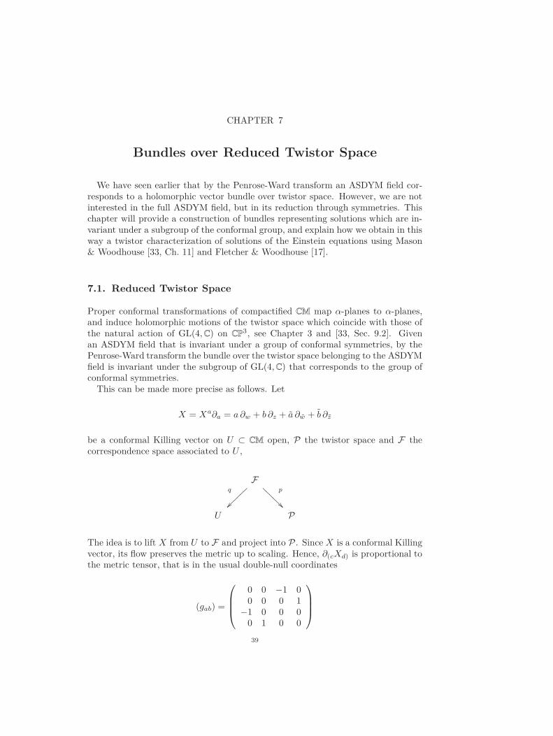
CHAPTER 7

Bundles over Reduced Twistor Space

We have seen earlier that by the Penrose-Ward transform an ASDYM field cor-responds to a holomorphic vector bundle over twistor space. However, we are notinterested in the full ASDYM field, but in its reduction through symmetries. Thischapter will provide a construction of bundles representing solutions which are in-variant under a subgroup of the conformal group, and explain how we obtain in thisway a twistor characterization of solutions of the Einstein equations using Mason& Woodhouse [33, Ch. 11] and Fletcher & Woodhouse [17].

7.1. Reduced Twistor Space

Proper conformal transformations of compactified CM map α-planes to α-planes,and induce holomorphic motions of the twistor space which coincide with those ofthe natural action of GL(4,C) on CP3, see Chapter 3 and [33, Sec. 9.2]. Givenan ASDYM field that is invariant under a group of conformal symmetries, by thePenrose-Ward transform the bundle over the twistor space belonging to the ASDYMfield is invariant under the subgroup of GL(4,C) that corresponds to the group ofconformal symmetries.

This can be made more precise as follows. Let

X = Xa∂a = a ∂w + b ∂z + a ∂w + b ∂z

be a conformal Killing vector on U ⊂ CM open, P the twistor space and F thecorrespondence space associated to U ,

Fq

⑦⑦⑦⑦⑦⑦ p

U P

The idea is to lift X from U to F and project into P . Since X is a conformal Killingvector, its flow preserves the metric up to scaling. Hence, ∂(cXd) is proportional tothe metric tensor, that is in the usual double-null coordinates

(gab) =

0 0 −1 00 0 0 1

−1 0 0 00 1 0 0

39

40 7. BUNDLES OVER REDUCED TWISTOR SPACE

the conditions

∂(wXw) = −∂(zXz) ⇔ ∂wa+ ∂wa = ∂zb+ ∂z b,

∂(wXz) = 0 ⇔ ∂za = ∂w b,

∂(wXw) = ∂(zXz) = 0 ⇔ ∂wa = ∂zb = 0,

∂(wXz) = 0 ⇔ ∂za = ∂wb,

(7.1)

together with the same equations but tilded and untilded variables interchanged.Now we are looking for a vector field X ′ that acts on α-planes and is induced by

the vector field X on U . So, we have to define a vector field X ′′ on F such that

q∗X′′ = X, (7.2)

and that preserves the distribution spanned by l, m, that is

[X ′′, l] = 0, [X ′′,m] = 0

modulo combinations of l and m. From (7.2) we see that X ′′ has to be of the form

X ′′ = a∂w + b∂z + a∂w + b∂z +Q∂ζ . (7.3)

For fixed ζ the conditions (7.1) imply

[X, l] = −lX = ζ(az∂w + bz∂z + az∂w + bz∂z)

− (aw∂w + bw∂z + aw∂w + bw∂z)

= ζ2az∂z + ζazl − bwm+ ζbz∂z − ζaw∂z − awl − bw∂z

= Q∂z mod (l,m)

whereQ = ζ2az + ζ(bz − aw) − bw. (7.4)

Similarly,[X,m] = Q∂w mod (l,m).

An easy calculation using (7.1) again shows also lQ = mQ = 0, hence [X ′′, l] =[X ′′,m] = 0. Therefore, with Q as in (7.4) we define X ′′ to be the lift of X fromU to F . Its projection X ′ = p∗X ′′ is a well-defined holomorphic vector field on thetwistor space, and the flow of X ′ is the action of conformal motions generated byX on α-planes.

Remember that λ = ζw+ z, µ = ζz+ w and ζ defined coordinates on the twistorspace and using w, z, w, z, ζ as coordinates on F the projection was given by

p : (w, z, w, z, ζ) 7→ (λ, µ, ζ) = (λ = ζw + z, µ = ζz + w, ζ).

Thus,X ′ = (ζa + b+ wQ)∂λ + (ζb + a+ zQ)∂µ +Q∂ζ

where the components are constant on α-planes, that is functions of λ, µ, ζ.Let U ⊂ CM be an open set satisfying the condition as in Theorem 4.2, and H be

a subgroup of the conformal group. We have shown that the Lie algebra h gives riseto Killing vectors X on U and to holomorphic vector fields X ′ on P . Now assumethat h acts freely on P , then we define the reduced twistor space R as the quotientof P over h.1 A vector bundle B′ → P , that is the Penrose-Ward transform of anASDYM connection D on a vector bundle B → U , is said to be invariant under hif it is the pullback of an unconstrained vector bundle E → R.

1A technically more detailed definition can be found in [33, Sec. 11.3].

7.1. REDUCED TWISTOR SPACE 41

In our example of stationary and axisymmetric solutions the reduction was gen-erated by the two commuting Killing vectors

X = w ∂w − w ∂w, Y = ∂z + ∂z.

The above construction yields

QX = −ζaw = −ζ, QY = 0.

This gives us

X ′′ = w∂w − w∂w − ζ∂ζ , Y ′′ = ∂z + ∂z ,X ′ = −µ∂µ − ζ∂ζ Y ′ = ∂λ + ζ∂µ.

With coordinates t, θ, x, r as in Chapter 5 and the gauge such that (5.5) holds,

Φ = −P dw

w+Q dz.2

The pullback of local invariant sections of a bundle E → P to F by p are simulta-neous solutions to

0 = Dls = ∂ls+ Φ(l)s = ∂ws− ζ(∂z +Q)s,

0 = Dms = ∂ms+ Φ(m)s = ∂zs− ζ(∂w − w−1P )s,

0 = X ′′(s), 0 = Y ′′(s)

(7.5)

where s is a function of ζ and the space-time coordinates. The first pair of equationsis required by the constancy of s on α-planes, and the second pair is the symmetrycondition.

Introducing the invariant spectral parameter σ = ζeiθ the symmetry conditionscan be stated as s = s(x, r, σ). A substitution of coordinates gives for the first pairof equations in (7.5) the form

(∂r − σ∂x + r−1σ∂σ)s− σ(J−1Jx)s = 0,

(∂x + σ∂r − r−1σ2∂σ)s+ σ(J−1Jr)s = 0,(7.6)

where J(x, r) is defined by

P = −rJ−1Jr, Q = J−1Jx.3

Equations (7.6) is a linear system for the reduced form of Yang’s equation that isintegrable if and only if (5.11) holds.

Another useful parameter for this example is

τ = x+1

2r(σ − σ−1) =

1

2(λ− ζ−1µ), (7.7)

which is constant along l and m as it depends only on λ, µ, ζ. Hence, τ is a functionon the twistor space.

The reduced twistor space has dimension 3−2 = 1, thus there exists one invariantcoordinate. Since

X ′τ = 0, Y ′τ = 0,

τ is constant along the orbits of X ′ and Y ′, so we can take it to be this coordinate.The pair of planes with σ = 0 and σ = ∞ corresponds to τ = ∞.

2This is a different Q as in the lift of the conformal Killing vector field.3Change of scale compared to (5.5).


The section s can now also be written in terms of x, r, τ , and the reduced systembecomes

(∂r − σ∂x)s− σ(J−1Jx)s = 0,

(∂r + σ∂x)s+ σ(J−1Jr)s = 0,

where σ is a function of x, r, τ by (7.7), and J satisfies the reduced form of Yang’sequation if and only if this reduced system is integrable for every τ .

A point of R is a leaf of the foliation of P spanned by X ′, Y ′. This is a two-parameter family of α-planes, each member being the orbit of one α-plane underthe flow of X ′ and Y ′. Points of R are labelled by τ .

The reduced twistor space R has a non-Hausdorff topology, which can be seen asfollows. Let U ⊂ CM as in Theorem 4.2, and P the twistor space of U . Consider aleaf of P , that is a point of R, with constant τ . This is the family of α-planes two ofwhich pass through a general point of U with coordinates t, θ, x, r, correspondingto the two roots of the quadratic equation

rσ2 + 2(x− τ)σ − r = 0 (7.8)

for σ. There are two cases. If we can continuously change one root into the other bymoving the point of U but keeping τ fixed, then there is only one leaf in the foliationfor this value of τ , hence τ labels a single point in R. Otherwise τ labels two points.

The discriminant of (7.8) is(x−τr

)2+ 1, so that there is only one solution to (7.8) if

τ = x± ir. Thus, τ labels only one point of U if τ = x± ir for some point of U , andtwo otherwise. For τ = ∞ we will always get two points, the leaves on which σ = 0and σ = ∞. If P is compact, then R as a quotient of P is compact, and from therange of the coordinate τ we see that it covers CP1. So, R is a compact Riemanniansurface covering CP1, but not Hausdorff, as for τ = x± ir with x, r belonging to apoint of the boundary of U there are two points in R. They cannot be separatedin the quotient topology since every neighbourhood contains a τ = x± ir for somepoint in U .

Despite our complex manifold not being Hausdorff it still makes sense in our caseto consider holomorphic vector bundles over it [49, App. 1].

7.2. The Twistor Construction

The considerations below are based on Fletcher & Woodhouse [17] which in turngo back to Woodhouse & Mason [49]. An alternative reference is Klein & Richter[28, App. B].

To obtain the formulae in the following in accordance with most of the literaturewe change the notation such that the coordinate −x is now named z, the param-eter −τ will be w as of now. Due to the clash with the standard notation fordouble-null coordinates this would have been confusing in the previous paragraphs.Furthermore, we will take ζ to be the spectral parameter instead of σ.

Another way of defining the reduced twistor space is to take the quotient of Uand F by h so that we have Σ = U/h and Fr = Σ × CP1. Then we obtain the

7.2. THE TWISTOR CONSTRUCTION 43

reduced version of the double fibration

Frq

~~⑦⑦⑦⑦⑦⑦

p

Σ Rwhich can be used for a slightly more abstract approach. Henceforth, instead ofbeginning with an ASD vacuum space-time, we take a two-dimensional complexconformal manifold Σ on which we are given a holomorphic solution r of the Laplaceequation. By z we denote the harmonic conjugate of r. We define Fr = Σ × X ,where X is a ζ Riemann sphere. The reduced twistor space R associated to Σ andr is constructed from Fr by identifying (σ, ζ) and (σ′, ζ′) if they lie on the sameconnected component of one of the surfaces given by

rζ2 + 2(w − z)ζ − r = 0 (7.9)

for some value of w and where z = z(σ), r = r(σ).We can use w as a local holomorphic coordinate on R, which is a non-Hausdorff

Riemann surface. Like above, w corresponds to one point of R if one can continu-ously change the roots of (7.9) into each other by going on a path in Σ and keepingw fixed; and two points otherwise.4 Let S be the w Riemann sphere, and V be theset of values for w which correspond only to one point in R. Then V ⊂ S is open,and if Σ is simply connected, then

V = z(σ) + ir(σ) : σ ∈ Σ. (7.10)

In general, V is not connected.However, for axis-regular solutions (for the definition see below) V can be enlarged

so that it becomes a simply connected open set V ′ ⊂ S. This situation is depictedin Figure 1. For w = ∞ we will always have two points, corresponding to ζ = 0

Im w = 0

Identified copies of V ′

∞0

S0 S1

∞1

Figure 1. Non-Hausdorff reduced twistor space with real poles(bullet points) as in the relevant examples.

and ζ = ∞, whatever x and r are. Therefore, w = ∞ is never in V . We denote thepoints in R corresponding to w = ∞ by ∞0 (for ζ = 0) and ∞1 (for ζ = ∞).

4Note that the condition for w to correspond only to one point is an open condition in R as z andr are smooth functions on Σ.


Now we need to construct the reduced form of the Penrose-Ward transform.First the forward direction, where we are given J as a solution of (5.11). In theunconstrained case the bundle over twistor space was defined by specifying what thefibres are. For an α-plane Z, that is a point in the twistor space P , it was the spaceof covariantly constant sections over Z in the given ASD bundle B → U (see endof Chapter 4). With our symmetry assumptions these are the sections defined by(7.5). We have seen above that with our additional symmetry (7.5) comes down to(7.6). Hence, the holomorphic bundle E → R is constructed by taking the fibre overa point of R to be the space of solutions of (7.6) on the corresponding connectedsurface in Fr. The integrability condition is precisely (5.11).

Conversely, let E → R be a holomorphic rank-n vector bundle together with achoice of frame in the fibres. For a fixed σ ∈ Σ let π : X → R be the restrictedprojection of Fr → R to σ×X , that is the identification (σ, ζ) ∼ (σ′, ζ′) as above,and denote by π∗(E) the pullback bundle of E to Fr. We have to assume that π∗(E)is a trivial holomorphic bundle over X .5

The matrix J can again be recovered within J 7→ AJB, where A and B areconstant, by the splitting procedure as in Chapter 4, but adapted to the symmetryconstraint. Suppose E is given by patching matrices Pαβ(w) according to anopen cover Rα of R such that ∞0 ∈ R0 and ∞1 ∈ R1. Then π∗(E) is given bypatching matrices

Pαβ(w(σ)) = Pαβ

(1

2r(σ)(ζ−1 − ζ) + z(σ)

)(7.11)

according to the open cover π−1(Rα) of X . The triviality assumption impliesthat there exist splitting matrices fα(ζ) such that

Pαβ

(1

2r(σ)(ζ−1 − ζ) + z(σ)

)= fα(ζ)f−1

β (ζ).6 (7.12)

We define J ≔ f0(0)f1(∞)−1. Another splitting would be of the form fαC for aninvertible matrix C, which has to be holomorphic on the entire ζ Riemann sphere,thus C is constant. But this leaves J invariant and the definition is independentof the choice of splitting. The splitting matrices fα depend smoothly on r, z as σvaries, so J does. Although J might have singularities where the triviality conditiondoes not hold.

Next we have to show that the so defined J satisfies (5.11). Therefore, we exploitthe freedom to choose the splitting matrices such that f1(∞) = 1, thus J = f0(0).Let Z1 = ∂r + ζ∂z + r−1ζ∂ζ and Z2 = −∂z + ζ∂r − r−1ζ2∂ζ be the vector fields in(7.6). An easy calculation shows Zi(w) = 0, i = 1, 2. Using this and acting withZi, i = 1, 2, on (7.12) yields for the left-hand side zero and hence for the right-handside

0 = Zi(fα)f−1β + fαZi(f

−1β ) = Zi(fα)f−1

β − fαf−1β Zi(fβ)f−1

β ,

which can be rearranged as

f−1α Zi(fα) = f−1

β Zi(fβ). (7.13)

In (7.13) the left-hand side is holomorphic on Rα and the right-hand side on Rβ ,so we obtain a function that is holomorphic on the entire ζ Riemann sphere, and

5This is less restrictive than it seems since if it is satisfied at one point σ then it holds in aneighbourhood of σ, compare comment on page 17.6See Proposition 2.5.

7.2. THE TWISTOR CONSTRUCTION 45

therefore by Liouville’s theorem both sides are independent of ζ. Evaluate (7.13)at ζ = 0, that is on R0. This can be written as

f−10 (0)Zi(0)(f0(0)) =

J−1∂rJ, i = 1

J−1∂xJ, i = 2.

But we can also write it as

f0(0)−1Zi(0)(f0(0)) = −Zi(f−10 (0))f0(0).

Combining both and rearranging yields

Zi(f−10 ) + (f−1

0 Zi(f0))f−10

∣∣ζ=0

= 0, i = 1, 2.

Therefore, f−10 is a solution for (7.6) at ζ = 0 and then for all ζ since we have

already seen that it is independent of ζ. The existence of a simultaneous solutionto both equations means they are integrable, thus J satisfies (5.11).

Another freedom in the construction of J from E is the change of local trivializa-tion Pαβ 7→ HαPαβH

−1β , where each Hα : Rα → GL(n,C) is holomorphic. Then J

becomes AJB with A = H0(∞0) and B = H1(∞1). This freedom of multiplying Jby constant matrices is the freedom of making linear transformations in the fibresof E over ∞0 and ∞1. By construction J is a linear map E∞1

→ E∞0, but in the

context of general relativity it was also the matrix of inner products of Killing vec-tors. Hence, E∞1

has to be interpreted as the space of Killing vectors in space-time,and E∞0

as its dual.Furthermore, from the context of general relativity we have the requirement for

J to be real and symmetric, and the constraint detJ = −r2. These conditionslead to further constraints on the bundle E → R which are in general still rathercomplicated [49, Sec. 5]. To obtain a simplification, we consider only axis-regularsolutions.

Definition 7.1. An Ernst potential J ′ is called axis-regular if the correspondingbundle E′ → RV satisfies E′ = η∗(E) where E is a bundle over R′ = RV ′ such

that E|S0and E|S1

are trivial.Here R′ is a double cover of the w-Riemann sphere identified over the two copies

of the set V ′ where V ′ is open, simply connected, invariant under w 7→ w andV ⊆ V ′ (V as in (7.10)). The map η : RV → RV ′ is the projection.

We shall also say that a metric J is axis-regular if the corresponding Ernst po-tential J ′ is.

Roughly speaking this definition just says that J ′ is axis-regular if we can enlargethe region where two spheres are identified to a simply connected patch such thatthis identification also extends to the fibres of E. The exact shape of V ′ is notimportant. Despite the further identifications we still have the projections Fr → R′

and can therefore construct J from a holomorphic bundle E′ → R′ that satisfiesthe triviality condition. Choose the copies of the two Riemann spheres in R′ suchthat ∞0 ∈ S0 and ∞1 ∈ S1.

If the bundle was not axis-regular, it meant that there are more than only isolatedpoints where the two spheres cannot be identified. Thus, in the light of later results(Proposition 8.16, Corollary 8.17) and [21, App. F] axis-regularity is necessary forthe the space-time not to have curvature singularities at r = 0.

This completes our construction of a correspondence between general relativityand twistor theory. The following diagram depicts the established relation in a


nutshell.

ASDYM connection forrank-(n− 2) vector bun-dle B → U

ooPW trf

Ch. 4

//

Ch. 7symmetry

reduction

B′ → P

Ch. 7symmetry

reduction

stationary axisymme-tric space-time of di-mension n

oocoincidence

Ch. 5

// reduced ASDYM oo

Ch. 7

// E → R

7.3. Review of the Four-Dimensional Case

For the rest of this chapter we review results for the case n− 2 = 2, that is J is a2 × 2-matrix and E a rank-2 vector bundle. To characterize the bundle E → R′ interms of patching matrices we choose a four-set open cover U0, . . . , U3 of R′ suchthat U0 ∪U2 ⊃ S0 with V ′ ⊂ U2 and ∞0 ∈ U0, and U1 ∪U3 ⊃ S1 with V ′ ⊂ U3 and∞1 ∈ U1. Now we use the following theorem.

Theorem 7.2 (Grothendieck). Let E → CP1 be a rank-a vector bundle. Then

E = Lk1 ⊕ . . .⊕ Lka = O(−k1) ⊕ . . .⊕ O(−ka)for some integers k1, . . . , ka unique up to permutation. Here, Lki = L⊗ki with Lthe tautological bundle.7

Hence we can choose a trivialization such that E|S0= Lp ⊕ Lq and E|S1

=

Lp′ ⊕ Lq

′

, that is

P02 =

(2w)p 0

0 (2w)q

, P13 =

(2w)p

′

0

0 (2w)q′

,

where we assume that without loss of generality w = 0 ⊂ V ′ which can beachieved by adding a real constant to w. The above form of the patching matricescan also be concluded from the Birkhoff factorization.

Now the triviality assumption and the symmetry imply that p = −p′ and q =−q′ which can be seen as follows. As a generalization of the winding number thedeterminant of a patching matrix has to be topologically invariant which impliesthat p + q is topologically invariant since detP02 ∼ wp+q . The triviality of thepullback of E to Fr then implies that p + q = p′ + q′. We will see later that thesymmetry of J requires that P02 = P−1t

13 , thus p = −p′ and q = −q′.That reduces the patching data to two integers p, q and a single holomorphic

patching matrix P (w) = P23(w) defined for w ∈ V ′. The remaining patchingmatrices are obtained by concatenation.

7O(1) is the tautological bundle: If z0 and z1 are linear coordinates on C2, then ζ = z1/z0 is

an affine (stereographic) coordinate on CP1. Each value of ζ, including ζ = ∞, defines a one-dimensional subspace Lζ ⊂ C2. So, as ζ varies, these subspaces form a line bundle L → CP1,

called tautological bundle O(1). Covering CP1 by V = z0, 0 and V = z1

, 0, we have atrivialization given by

t([z], λ(z0, z1)) = ([z], λz0) and t([z], λ(z0, z1)) = ([z], λz1)

so that the transition function is z1/z0 = ζ.

7.3. REVIEW OF THE FOUR-DIMENSIONAL CASE 47

We can then also reduce the reconstruction of J from E′ → R′ given p, q and P .For fixed r, z we get a map π : X → R′ by

ζ 7→ w =1

2r(ζ−1 − ζ) + z, (7.14)

where X is again the ζ Riemann sphere, namely (r, z) × X ⊂ Fr. The map is notyet well-defined as outside V ′ a value of w corresponds to two points of R′. So, wehave to add a rule which of the two points is to be π(ζ). For the construction ofJ(z, r) we need z ± ir to be in V ′, otherwise π is only a double cover of one of thespheres in R′ (ζ = 0 and ζ = ∞ lie on different spheres) for the following reason.First note that ζ and −ζ−1 are mapped to the same w, so if w < V ′ it correspondsto two points, each on one sphere, and we have to decide to which sphere we map ζand −ζ−1. Note further, as soon as we can find a path from ζ to −ζ−1 whose imagedoes not go through V ′, π covers only one sphere, because we can only change thesphere by going through V ′. Now the image of every path from ζ to −ζ−1 has togo through one of the points w = z + ir as ζ and −ζ−1 lie on different branches ofthe root function of quadratic equation (7.14), hence the path has to go througha branch point. Any other value of w can be avoided by picking a suitable path.Thus, if w = z + ir < V ′, then we can find a path connecting ζ and −ζ−1 whoseimage does not go through V ′ and π must be a double cover of one of the spheres.However, as we have seen above, if r = r(σ) and z = z(σ) for σ ∈ Σ this conditionis satisfied automatically (which will be assumed further on).

If V ′ is simply connected, π can be fixed by the condition that ζ = 0 is mappedto ∞0 ∈ S0 and ζ = ∞ to ∞1 ∈ S1. Yet, even if the space-time is regular on r = 0,that is there exist smooth non-singular coordinates on a neighbourhood of r = 0,the Ernst Potential may have poles on r = 0 (see Example 6.8). In most of therelevant examples V ′ is the complement of a finite set — infinity and a finite set ofisolated singularities, V ′ = CP1\∞, w1, . . . , wn, where the wi lie on the real axis,thus, suppose V ′ is not simply connected. The wi correspond to two points of X ,the roots of

rζ2 + 2(wi − z)ζ − r = 0, (7.15)

where r and z are still fixed. Here we need to assign the roots to S0, S1, say π(ζ0i ) ∈

S0 and π(ζ1i ) ∈ S1. Choose a cover V0, V1 of X such that 0, ζ0

1 , . . . , ζ0n ⊂ V0 and

∞, ζ11 , . . . , ζ

1n ⊂ V1. To define J(z, r) we use what is called the Ward ansatz in

Woodhouse & Mason [49, Sec. 5.5]. With given patching data p, q and P we havepatching matrices

P02 = P−113 =

(2w)p 0

0 (2w)q

, P23 = P.

Now instead of looking for splitting matrices for P01, we first do a transformationto our patching matrices. Let m0 = 2ζw

rand m1 = − 2w

ζr, and define

M0 =

m−p

0 0

0 m−q0

, M1 =

mp

1 0

0 mq1

, M2 =

rpζ−p 0

0 rqζ−q

.

Then Mα(ζ), α = 0, 1, is holomorphic and invertible on Uα and M2 is holomorphicand invertible on U2 and U3. Furthermore, since

m0(0) =2ζ

r

(1

2r(ζ−1 − ζ) + z

)∣∣∣∣ζ=0

= 1,


and similarly m1(∞) = 1, we get M0(0) = M1(∞) = id so that J(z, r) is unchangedby using Pαβ = MαPαβM

−1β instead of Pαβ . Yet, P02 = 1, which means we can

reduce our open cover to U ′0 = U0 ∪ U2 and U ′

α = Uα, α = 1, 3. For the evaluationof J(z, r) we seek a splitting Q0(ζ) and Q1(ζ) of the new patching matrix P ′

01 whichis

P ′01 = M0P01M

−11 = M0P02P23P31M

−11

=

rpζ−p 0

0 rqζ−q

P

(1

2r(ζ−1 − ζ) + z

) (−rζ)p 0

0 (−rζ)q

= Q0Q−11 .

(7.16)

Here Q0, Q1 are holomorphic in ζ and non-singular in V0 and V1, respectively. Asbefore, we set J ≔ Q0(0)Q−1

1 (∞), and obtain a solution of (5.11). A different label-ing of the roots of (7.15) yields a different solution J , yet these different solutionsare analytic continuations of each other and one can show that they are differentparts of the Penrose diagram of the maximal analytic extension of the metric (thiswill be considered again in Chapter 8 from a slightly different point of view).

From the interpretation of J as the matrix of inner products of Killing vectors ingeneral relativity, we require J to be real and symmetric. Therefore, the questionsarises which conditions we have to impose on our bundle to obtain solutions withthe desired properties. The following can be immediately read off from the splittingprocedure in any dimension (restriction to n = 2 not necessary).

Let i be the map that interchanges the spheres, that is it is the identity on V ′

and otherwise the two points of R′ that correspond to the same w are interchanged.Then J−1 is obtained from the pullback bundle i∗(E) and furthermore J−1t isobtained from the dual bundle E∗. Hence,

J = J t ⇔ J−1 = (J−1)t ⇔ i∗(E) = E∗ ⇔ P−1 = (P−1)t ⇔ P = P t,

or in other words J is symmetric, which means J = J t, if and only if P = P t, thatis P is symmetric.

Remember in general for a holomorphic function ϕ(a) we have that ϕ is real on the

real numbers if and only if ϕ(a) = ϕ(a). So, if P is real in the sense P (w) = P (w),then by (7.16) we have

P (w) = P (w) ⇒

Q0(ζ) ·Q1(ζ)

−1= Q0(ζ)Q1(ζ)−1, r, z ∈ R;

Q0(ζ) ·Q1(ζ)−1

= Q0(−ζ)Q1(−ζ)−1, z ∈ R, r ∈ iR.

So, J must be real as well, provided r, z ∈ R or z ∈ R, r ∈ iR. In terms of thebundle this is the condition E = j∗(E) where E is the complex conjugate bundleof E and j∗(E) is the pullback with the complex conjugation on the spheres

j :S0 → S0, w 7→ w;

S1 → S1, w 7→ w.

The converse, that is a real J implies a real P , is then also obvious.Moreover, for n = 2 it can be shown that (see for example [49], but as cited here

it is taken from [17]):

• If detP = 1, then detJ =(−r2

)p+q.

7.3. REVIEW OF THE FOUR-DIMENSIONAL CASE 49

• If J is obtained from an axis-regular space-time and if the definition of πis such that ζ0

i → 0 and ζ1i → ∞ for r → ∞ and all i, then p = 1, q = 0

and P (z) = J ′(z, 0) on the rotational axis or on the horizon. Here, J ′ isthe Ernst potential. Thus, P is the analytic continuation of the boundaryvalues of the Ernst potential.

As an argument in Fletcher [16] shows, this can be seen from thedeterminant condition above and the fact that J is bounded on the axis.The determinant condition implies p + q = 1 and an asymptotic relationbetween J and P reveals that if J is bounded as r → 0 then p and q mustbe non-negative. So, either p = 1, q = 0 or p = 0, q = 1. We can assumethat the trivialization over S0 and S1 can be chosen such that the firstholds. The same argument implies that the twistor data obtained from J ′

has p = q = 0, since det J ′ = 1. This goes along with the interesting effectthat the gauge groups for J and J ′ (in their Yang-Mills interpretation) aredifferent [49, Sec. 6].

• If J comes from an asymptotically flat space-time in the sense that itsErnst potential has the same asymptotic form as the Ernst potential ofMinkowski space with rotation and translation as Killing vectors, thenP (∞) = 1, and conversely.

These results can be used to look at some examples.

Example 7.3.

(1) Minkowski Space with Translation and RotationWritten in cylindrical polar coordinates

ds2 = dt2 − r2 dθ2 − dr2 − dz2

we can take the Killing vectors to be X = ∂θ, Y = ∂t. The matrix of innerproducts and the Ernst potential are then

J =

(−r2 0

0 1

), J ′ =

(1 00 1

).

Since it is axis-regular we also have p = 1 and q = 0 with V ′ the entirecomplex plane.

(2) The Kerr solutionThe patching data for the Kerr solution is (without proof)

P (w) =1

w2 − σ2

(w + m)2 + a2 2am

2am (w −m)2 + a2

where σ =√m2 − a2 for a < m. Axis-regularity implies again p = 1 and

q = 0. The open set V ′ is the complement of ∞, w1, w2 where w1 = σand w2 = −σ.

CHAPTER 8

Twistor Approach in Five Dimensions

Most of what we have seen about the twistor construction at the end of Chapter 7generalizes without any effort to five and higher dimensions. Only, instead of two,the rank of the bundle will be three so that we have three integers instead of onlyp and q in our twistor data (respectively n− 2 in higher dimensions). The splittingprocedure itself is not affected by increasing the rank. However, since the splittingitself is complicated, we have seen that the Ernst potential J ′ is a crucial tool forany practical application of the twistor characterization of stationary axisymmetricsolutions of Einstein’s field equations, and the way we obtained J ′ in Chapter 5seemed to be tailored to four dimensions with two Killing vectors. So, in order topursue this strategy we have to define an Ernst potential in five dimensions. First,we are going to say a few words about Bäcklund transformations, because we willsee that we secretly used them to obtain J ′. Since some of the following extendsimmediately to higher dimensions as well, we will present most of it in n dimensions.

In the last part of this section we generalize results from Fletcher [16, Sec. 2.4]in order to conclude the important fact that the integers in the twistor data arenon-negative as in four dimensions.

8.1. Bäcklund Transformations

In Chapter 5 we derived Yang’s equation as one way of writing the ASDYM equa-tions with gauge group GL(n,C). It has a number of ‘hidden’ symmetries one ofwhich is the Bäcklund transformation.

As in Mason & Woodhouse [33, Sec. 4.6] we can decompose a generic J-matrixin the following way1

J =

A−1 − BAB −BA

AB A

=

1 B

0 A−1

−1 A−1 0

B 1

, (8.1)

where A is a k×k non-singular matrix (k < n), A is k× k non-singular matrix withk+ k = n. Then, B is a k×k and B a k× k matrix. The term ‘generic’ rules out forexample cases where A is not invertible. Substituting this in Yang’s equation (5.2)

1Using

(1 B

0 A−1

)−1

=

(1 −BA

0 A

).

51

52 8. TWISTOR APPROACH IN FIVE DIMENSIONS

we get the coupled system of equations

∂z(ABzA) − ∂w(ABwA) = 0,


∂z(A−1Az)A

−1 − ∂w(A−1Aw)A−1 +BzABz −BwABw = 0,

A−1∂z(AzA−1) −A−1∂w(AwA

−1) + BzABz − BwABw = 0,

(8.2)

where an index denotes a partial derivative (see Appendix I for detailed calculation).The first two equations are integrability conditions and they imply the existence ofmatrices B′ and B′ such that

∂zB′ = ABwA, ∂wB

′ = ABzA,

∂zB′ = ABwA, ∂wB

′ = AB zA.

Definition 8.1. Together with B′ and B′ we define the other primed quantitiesas (

A, A,B, B, k, k)

7→(A′ = A−1, A′ = A−1, B′, B′, k′ = k, k′ = k

).

We call the matrix J ′, that is obtained from J by (8.1) with the primed blocksinstead of the unprimed, the Bäcklund transform.

Proposition 8.2 (Section 4.6 in Mason & Woodhouse [33]).

(1) J ′ is again a solution of Yang’s equation.(2) (J ′)′ = J

Proof.

(1) Substitute the unprimed by the primed versions in (8.2).(2) Noting that Bw = A−1B′

zA−1 = A′B′

zA and similar for the other integra-bility equations, this statement is obvious.

However, the connection between ASDYM and Einstein’s field equations in thestationary and axisymmetric case was given by the reduced Yang’s equation

r∂x(J−1∂xJ) + ∂r(rJ−1∂rJ) = 0,

see (5.11). The reduction was induced by the coordination transformation

z = t+ x, z = t− x, w = reiθ, w = re−iθ.

Now we have to be careful, because the r-derivatives also act on the r-factors ap-pearing. But an analogous calculation as above (see Appendix J) shows that thereduced Yang’s equation is equivalent to a similar set of equations

r∂x(ABxA) + ∂r(rABrA) = 0,

r∂x(ABxA) + ∂r(rABrA) = 0,

r∂x(A−1Ax)A−1 − ∂r(rA−1Ar)A

−1 + rBrABr − rBrABr = 0,

rA−1∂x(AxA−1) −A−1∂r(rArA

−1) + rBrABr − rBrABr = 0,

(8.3)

where all matrices are functions of x and r. The integrability conditions are now

∂rB′ = rABxA, ∂xB

′ = −rABrA,

∂rB′ = rABxA, ∂xB

′ = −rABrA.

8.2. HIGHER-DIMENSIONAL ERNST POTENTIAL 53

So, we have to adapt the transform, namely we define A′ = r−2A−1, A′ = A−1

and the rest as above2. Again by substitution it can be checked that this givesa solution of the reduced Yang’s equation. However, one should note that thismodified Bäcklund transformation is not an involution anymore since the definitionfor A′, A′ is not involutive. The definition for B′, B′ is still an involution sothat the inverse Bäcklund transformation is obtained by B = B′′, B = B′′ andA = r−2(A′)−1, A = (A′)−1.

Proposition 8.3.

detJ ′ = (−r)2(1−k)

Proof. Note that for the decomposition of a general matrix in block matriceswe know from basic linear algebra

det

(P QR S

)= det(S) det(P −QS−1R),

if S is invertible. Applied to our decomposition (8.1) this yields

detJ = det(A) det(A−1 − BAB + BAA−1AB) = det(A) det(A−1). (8.4)

Now using the fact that detJ = −r2 we obtain

detJ ′ = det(A′) det((A′)−1)

= (−r)−2k det(A−1) det(A)

= (−r)−2k det(J)

= (−r)2(1−k)

Example 8.4 (Bäcklund Transformation in Four Dimensions). As in [33,Sec. 6.6], we consider the four-dimensional case with two Killing vectors. As in(5.21) we set A = −r−2f , A = f , B = −B = α. Then the integrability equationstake the form

∂x(r−1f2∂xα) + ∂r(r−1f2∂rα) = 0,

like in (5.22). The blocks for the Bäcklund transform are B′ = −B′ = ψ, A′ =A−1 = f−1, A′ = −r−2A−1 = f−1 defining

J ′ =1

f

(f2 + ψ2 ψ

ψ 1

),

where the existence of ψ is ensured by the integrability condition as above. Hence,our Ernst potential is obtained by a Bäcklund transformation.

8.2. Higher-Dimensional Ernst Potential

Let us first recall the definition of twist 1-forms, twist potentials and some of theirproperties.

2Note that this modification is not mentioned in [33, Sec. 4.6], but necessary to obtain the correctresult in Example 8.4.


Definition 8.5. Consider an n-dimensional (asymptotically flat) space-time Mwith X0 a stationary and X1, . . . , Xn−3 axial Killing vectors, all mutually commut-ing. The twist 1-forms are defined as

ω1a = ∆ εab...cdeXb1 · · ·Xc

n−3∇dXe1 ,

...

ωn−3,a = ∆ εab...cdeXb1 · · ·Xc

n−3∇dXen−3,

where ∆ =√−g = re2ν , according to (5.18).3

Adopting a vector notation

ω =

ω1...

ωn−3

, X =

X1...

Xn−3

this can be written as

ωa = ∆ εab...cdeXb1 · · ·Xc

n−3∇dXe.

Let θI , I ∈ 1, . . . , n− 3, be the dual to XI , that is θIk = gkjXjI .

Proposition 8.6.

(1) The twist 1-forms can be written as

ωI = ∗(θ1 ∧ . . . ∧ θn−3 ∧ dθI), I ∈ 1, . . . , n− 3. (8.5)

(2) ω is closed.(3) ω annihilates the Killing vector fields X0, . . . , Xn−3.

Proof.

(1) Suppressing the I-index for θ, we note that

∇[dθe] = ∂[dθe] − Γf[de]θf = ∂[dθe]

as we use the Levi-Civita connection for which Γfde

= Γf(de). But ∂[dθe] are

the components of dθ so that from the definition of the Hodge dual we seethat (8.5) is an equivalent way of writing the twist 1-forms.

(2) Analogously to the proof of [45, Thm. 7.1.1] implied by the vacuum fieldequations.

(3) We denote by xK the coordinate belonging to XK , K = 0, . . . , n− 3, andfor M/G we use again r and z as coordinates. It is sufficient to show thatω = ωr dr + ωz dz with all other components vanishing. We will do thefollowing calculations a bit more in detail as the results will proof usefullater on. Using

θIk = gkaXaI = JkI for I = 1, . . . , n− 3,

3Note that in [24] the notation is taken from [45] where ε is already the volume element.


we first calculate

dθI = ∂rJ0I dr ∧ dx0 + . . .+ ∂rJn−3,I dr ∧ dxn−3

+ ∂zJ0I dz ∧ dx0 + . . .+ ∂zJn−3,I dz ∧ dxn−3

= −(∂rJ0I dx0 + . . .+ ∂rJn−3,I dxn−3) ∧ dr

− (∂zJ0I dx0 + . . .+ ∂zJn−3,I dxn−3) ∧ dz.

This gives for I ∈ 1, . . . , n− 3 the following

θ1 ∧ . . . ∧ θn−3 ∧ dθI = −(JK1 dxK) ∧ . . . ∧ (JM,n−3 dxM )

∧((∂rJRI dxR) ∧ dr + (∂zJRI dxR) ∧ dz

),

where the summation over capital latin indices runs from 0 to n − 3. Atthis point we can already see that only ωr, ωz are non-zero, but let usdetermine them somewhat more precisely. Our volume form is

dvol = r dx0 ∧ . . . ∧ dxn−3 ∧ (ω dr) ∧ (ω dz),

so that

∗(r dx0 ∧ . . . ∧ dxn−3 ∧ (ω dr)

)= (−1)n−2ω dz,

since the left-hand side contains n− 2 spacelike and one timelike compo-nent. Thus

∗(dx0 ∧ . . . ∧ dxn−3 ∧ dr

)= (−1)n−2 1

rdz;

similar for dr ↔ dz but with the opposite sign. Whence we obtain

ωIr = (−1)n−1 1

r

∑

σ∈Sn−2

sgn(σ)J1,σ(0) · · · Jn−3,σ(n−4)∂zJI,σ(n−3)

= (−1)n−1 1

rdet

J01 · · · J0,n−3 ∂zJ0I

.... . .

......

Jn−3,1 · · · Jn−3,n−3 ∂zJn−3,I

, (8.6)

where Sn−2 are the permutations of n−2 elements. An analogous equationholds for ωIz.

The last statement in the above proposition implies that ω can also be regardedas 1-forms on the interior of M/G. Due to the form of the σ-model metric thereshould be no confusion if we denote both the form on M and the one on M/Gby the same symbol. Being a form on M/G means that ω has only non-vanishingcomponents for the r- and z-coordinate, and of course as a form on M/G it willagain be a closed. This gives rise to the following definition.

Definition 8.7. Locally there exist functions on M/G such that

∂rχI = ωIr and ∂zχI = ωIz for I = 1, . . . , n− 3,

or equivalently in vector notation

dχ = ω.

These functions χI are called twist potentials.


The construction of the Ernst Potential in Example 8.4 is tailor-made for dimen-sion four, and it is not immediately obvious how to generalize it to higher dimen-sions. Nevertheless, there is an ansatz in Maison [31], where it is noted that the fullmetric on space-time, that is essentially J , can be reconstructed from knowing thetwo twist potentials (in five dimensions) χ, the 2×2-matrix A =

(XaIX

bKgab

)I,K=1,2

and its non-vanishing determinant det A on the factor space M/G. The matrix in[31, Eq. (16)] will then be our candidate for the higher-dimensional Ernst Potential.Note, however, that the condition det A , 0 needs further investigation.

Closely connected to the non-vanishing determinant is the concept of adaptationsto certain parts of the axis r = 0. Recall that the assumption of axis-regularity wasan important one. It said that the region where the two spheres of the reducedtwistor space are identified can be enlarged to a simply connected patch such thatthis identification also extends to the fibres of the bundle. The exact shape of V ′

is not important, however, there is still an ambiguity if we have a nut on r = 0.4

Figure 1 shows how we can choose different extensions of V . From Example 6.8 we

Im w

Re w

V ′1

V

V

V ′2

Figure 1. Two different extensions V ′1 and V ′

2 of V around a poleof J ′ (bullet on the real axis).

learn that the choice of V ′ matters, that is we obtain different Ernst potentials J ′

for different extensions.

Definition 8.8. In any dimension given an axis-regular J ′ we shall call it adaptedto the rod (ai, ai+1) if V ′|r=0 ⊆ (ai, ai+1).

For a rod corresponding to a rotational axis we know that along this rod a linearcombination of the axial Killing vectors vanishes. By a change of basis we canalways assume that without loss of generality this vector is already in the basis, sayXK = 0, K > 0. Then we make the following definition.

4Remember that we assume that there is only a finite number of isolated nuts.


Definition 8.9. In dimension n we call A adapted to (ai, ai+1) the (n−3)×(n−3)-matrix that is obtained from J by

(a) cancelling the Kth column and row, if (ai, ai+1) is a rotational axis and XK thecorresponding rod vector;

(b) cancelling the 0th column and row, if (ai, ai+1) is the horizon.

The following lemma shows the reason for the latter definition.

Lemma 8.10. A adapted to (ai, ai+1) is invertible on (ai, ai+1) and becomes sin-gular at the limiting nuts.

Proof. This is a simple consequence of what we have seen in Section 6.2.First, consider a rod corresponding to a rotational axis (ai, ai+1). Here J is an(n−2)×(n−2) matrix and has rank n−3. Since XK = 0 on (ai, ai+1), we cancelled azero column and row, thus it follows that A has full rank and det A , 0 on (ai, ai+1).Of course, where the rank of J drops further, that is where dim kerJ(0, z) ≥ 2, thematrix A cannot have full rank anymore and det A = 0. So, this adaptation becomessingular as soon as we reach one of the nuts limiting this rod.

Second, consider the horizon rod (ah, ah+1). Here the first row and column of J ,that is the one with the asymptotically timelike Killing vector in it, becomes zero.Then A adapted to (ah, ah+1) has full rank on (ah, ah+1), and becomes singular atthe nuts where the rotational axes intersect the horizon.

Note that at the beginning of this section we defined the twist 1-forms bysingling out X0. However, the definition works just as well with the setX0, . . . , XK , . . . , Xn−2 of Killing vectors. For an adaptation to a certain rod weobtain in the same way as above n− 3 twist potentials by omitting the rod vectorfor this rod.

Now, we have collected all the components for the following definition, which isa modification of [31, Eq. (16)].

Definition 8.11. In n dimensions and for a given rod (ai, ai+1) we call thematrix

J ′ =1

det A

1 −χt


, (8.7)

where A is adapted to (ai, ai+1) and χ is the vector of twist potentials for (ai, ai+1),higher-dimensional Ernst potential adapted to (ai, ai+1).

Remark 8.12.

(1) For n = 5 this is becomes on the horizon rod

J ′ =1

det A

1 −χ1 −χ2

−χ1 det A · J11 + χ21 det A · J12 + χ1χ2

−χ2 det A · J21 + χ2χ1 det A · J22 + χ22

.

(2) Note that J =(g(Xi, Xj)

)is a matrix of scalar quantities, hence J is

bounded for r → 0. So, the domain of J ′ is only restricted by det A andby the arguments above we see that for an adaptation to (ai, ai+1) thelimit J ′(0, z) is well-defined for z ∈ (ai, ai+1).


Lemma 8.13 (Maison [31]). J ′ = (J ′)t, detJ ′ = 1 and

(J ′)−1 =

χtA−1χ+ det A χtA−1

A−1χ A−1

.

Proof. The first part is obvious, the second part is an easy calculation andProposition 8.3 implies for k = 1 that detJ ′ = 1.

Even though ingredients and the matrix J ′ itself were known already before, thecrucial new step for the twistor construction is to recognize the following.

Theorem 8.14. J ′ is obtained from J by a Bäcklund transformation.

Proof. Consider without loss of generality J ′ adapted to the horizon. Wedecompose J according to (8.1)

J =

A−1 − BAB −BA

AB A

with A as above the spatial part of J ,

B = −Bt = A−1

J01...

J0,n−3

,

and k = 1, k = n−3. In order to calculate A remember that the inverse of a generalmatrix was given

A−1 =1

det A(A)t,

where A =((−1)i+j det(Aij)

)with Aij being the matrix obtained from A = (Aij)

by crossing out the ith row and jth column.As a first step towards A we do a Laplace expansion of det J along the first row

detJ = J00 det A+n−3∑

k=1

(−1)k+2J0k det J0k,

and by another Laplace expansion (also using that J is symmetric)

det J0k =

n−3∑

l=1

(−1)l+1J0l det Akl.

Substituting the latter one in the expression for det J yields

detJ = J00 det A−n−3∑

k,l=1

(−1)k+lJ0k det AklJ0l

= J00 det A− det A(J01 · · · J0,n−3

)A−1

J01...

J0,n−3

,

which is equivalent todetJ

det A= J00 + BtAB = A−1.


Hence

A =det A

detJ= −r−2 det A,

and we can, in line with the Bäcklund transformation, define

A′ = A−1, A′ = −r−2A−1 = det A−1.

To complete our proof of showing that J ′ is a Bäcklund transform we have to verifythat the integrability conditions yield the right expression for the twist potentials.They take the form

∂rB′ = r−1 det(A)A ∂z

A−1

J01...

J0,n−3

,

∂zB′ = −r−1 det(A)A ∂r

A−1

J01...

J0,n−3

,

and B′ = −(B′)t. We are done if we can show that B′ = χ because then ourconstructed J ′ coincides with the Bäcklund transform (apart from swapping thefirst and last row, respectively column, which does not affect our considerations).

So, it remains to show

∂rχ = ωr = r−1 det(A)A ∂z

A−1

J01...

J0,n−3

,

∂zχ = ωz = −r−1 det(A)A ∂r

A−1

J01...

J0,n−3

.

(8.8)

Starting from the left-hand side of (8.8) we Laplace expand the determinant in(8.6) twice; first along the last column and then along the first row

r · ωIr = (−1)n−1(−1)1+(n−2)∂zJ0I · det A

+ (−1)n−1n−3∑

l=1

(−1)(l+1)+(n−2)∂zAl,I · det

J01 · · · J0,n−3

......

Jl,1 · · · Jl,n−3

......

Jn−3,1 · · · Jn−3,n−3

= ∂zJ0I · det A+

n−3∑

l=1

(−1)l∂zAlI

(n−3∑

k=1

(−1)k+1J0k · det Akl

)

= det A

∂zJ0I −

(∂zA1I · · · ∂zAn−3,I

)A−1

J01...

J0,n−3

.


However, the last line is the Ith component of

r · ωr = det A

∂zJ01...

∂zJ0,n−3

− (∂zA)A−1

J01...

J0,n−3

= det A · A ∂z

A−1

J01...

J0,n−3

,

which corresponds to the right-hand side of (8.8). An analogous computation veri-fies the second equation of (8.8).

This completes the justification to call the J ′ defined in (8.7) Ernst potential —by Proposition 8.2 it satisfies Yang’s equation and by Lemma 8.13 it is symmetricand has unit determinant.

8.3. Properties of P and the Bundle

Having different adaptations of J ′ which are related to different extenstions of Vthe question arises whether these yield equivalent bundles over the reduced twistorspace. To see that is true is not very hard using results in Fletcher [16].

Proposition 8.15 (Proposition 3.1 in Fletcher [16]). Suppose E → RV , the bun-dle corresponding to a solution J of Yang’s equation on the set V , can be representedas the pullback of the bundles E1 → RV ′

1and E2 → RV ′

2, where V ′

1 and V ′2 are sim-

ply connected open sets which intersect the real axis in distinct intervals. Then E1

and E2 are the pullbacks of a bundle E → RV where V = V1 ∪ V2. Moreover, we

can express E in standard form in two different ways; and one of the collectionsof patching matrices is identical to the collection used to describe E1 and the othercollection is identical to that used to describe E2.

Sketch of Proof. The proof in Fletcher [16] only makes use of the construc-tion for the reduced twistor space and not of the rank of the bundle. So, it carriesover to higher dimensions.

Roughly speaking the argument is that for two different adaptations with reducedtwistor spaces RV1

and RV2, as in Figure 1, their pullbacks to RV have to be

equivalent (in the sense of Proposition 2.5), since in both cases it yields the bundledefined by the solution J for (5.11). But if they are equivalent on RV and are bothanalytical continuations, then they have to belong to the same bundle and are onlytwo different representations of it.

The bridge between Ernst potential and patching matrix is built by analyticcontinuation.

Proposition 8.16 (Proposition 7.2 in Woodhouse & Mason [49]). In five as wellas in four dimensions if P is a patching matrix of an axis-regular Ernst potentialJ ′ on V , then J ′ is analytic on (a choice of) V ′ and J ′(0, z) = P (z) for real z.

Proof. This is literally the same as for Woodhouse & Mason [49], since it doesnot make use of the rank of the bundle. Note that even though in the statementthere the assumption of J being positive definite is made, it in fact is not necessaryfor the proof.

8.4. PATCHING MATRIX NEAR THE AXIS 61

Corollary 8.17. A patching matrix P has real singularities, that is points z ∈ Rwhere an entry of P has a singularity, at most at the nuts of the rod structure.

Proof. Suppose P corresponds to the bundle E → RV , where V is the max-imally extended region over which the spheres can be identified. Suppose furtherthat P has a real singularity a ∈ R which is not one of the nuts, say without lossof generality a ∈ (ai, ai+1). Then from Proposition 8.15 we know that E can onVi be expressed in standard form. But using Proposition 8.16 that means thatP (z) = J ′

i(z, 0) for z ∈ (ai, ai+1). On the other hand we have seen earlier alreadythat J ′

i is regular on (ai, ai+1) and only becomes singular when approaching thenut. Contradiction!

For every other bundle E → RV it must be V ⊆ V , hence E is the pullback of Eand as such the patching matrix of E cannot have poles where the patching matrixof E has not.

As in Fletcher [16] we sometimes also call the singularities of P double points,because the singularities of P are the points where the two Riemann spheres of thereduced twistor space cannot be identified.

Proposition 8.18. The real singularities of a patching matrix P are simple poles.

Proof. We have seen above that on the real axis r = 0 the singularities of Pare caused by the term det A. So, consider the rod (ai, ai+1) where A has full rank.The determinant of a matrix equals the product of its eigenvalues. Furthermore,towards the nuts ai, ai+1 we know, also from above, that the rank of A dropsprecisely by one which is the case if and only if det A contains the factors z − aiand z − ai+1, respectively, with multiplicity one.

Note that if P has a pole with r , 0, then it is obviously not splittable at thispoint, see (7.12), hence we do not obtain J at this point by the splitting procedurewhich means the metric might be singular at this point. We would like to excludesuch situations. However, referring again to (7.12) it is evident that the splittingprocedure in general does break down for r → 0. So, one has to study this limitby means of other tools, see Section 8.4, and we have seen in Example 6.8 even forregular space-times it is possible that P has real poles. But as in Chapter 7 weassume that there are only finitely many of them.

8.4. Patching Matrix near the Axis and Twistor Data Integers

In this last part we will sketch a generalization of the asymptotic formula of J forr → 0. Originally, the result in four dimensions goes back to Ward [46], but herewe will follow the lines of Fletcher [16, Sec. 2.4].

In Section 8.2 we defined

J ′ =

g −gχt

−gχ A+ g · χχt

,

where g = (det A)−1. We have shown above that P (w) is the analytic continuationof J(r = 0, z), hence we can assume that it also takes the form

P (w) =

g −gχt

−gχ A+ g · χχt

,


but the entries being functions of w. Analogously to Chapter 7 we have

P02 = P−113 = diag

((2w)p0 , (2w)p1 , (2w)p2

), P23 = P.

Furthermore, we assume for the integers p0 ≥ p1 ≥ p2, which is just a question ofordering. Following exactly the lines as in Chapter 7 we obtain

Q0Q−11 =

(r

ζ

)p0

(r

ζ

)p1

(r

ζ

)p2

P (w)

(−rζ)p0

(−rζ)p1

(−rζ)p2

,

where the left-hand side is a function of ζ. With

R01 =

ζ−p0

ζ−p1

ζ−p2

P (w)

(−ζ)p0

(−ζ)p1

(−ζ)p2

this can be rewritten as

Q0Q−11 =

rp0

rp1

rp2

R01

rp0

rp1

rp2

.

Suppose we can split g = g0g−11 , where g0 is holomorphic in ζ, that is on S0, and

g−11 is holomorphic in ζ−1, that is on S1. This may be achieved by the use of a

Laurent series. We claim that then R01 can be split as follows

R01 =

ζ−p0

ζ−p1

ζ−p2

(

g0 0

− g0χ A0

)ζp0

ζp1

ζp2

︸︷︷︸≕M

0(ζ)

×

ζ−p0

ζ−p1

ζ−p2

(g−1

1 −g−11 χt

0 A−11

)

(−ζ)p0

(−ζ)p1

(−ζ)p2

︸︷︷︸≕M−1

1(ζ)

,

where A0 is holomorphic in ζ, that is on S0, and lower triangular, and A−11 is

holomorphic in ζ−1, that is on S1, and upper triangular. All these steps generalizestraight-forwardly to more than five dimensions. In the case of n dimensions therange of integers is p0 ≥ . . . ≥ pn−3. In the following paragraphs it does notsimplify the notation if we restrict to n = 5, therefore we will consider the moregeneral setting.

The matrices M0, M1 are not necessarily holomorphic and non-singular on S0 orS1, respectively. Yet, we can expand χ(w) and the off-diagonal entries of A0(w)around w = z which yields5

χ(w) =

∞∑

k=0

χ(k)(z)rk

2kk!(ζ−1 − ζ)k,

and similarly for the entries of A0(w). Here χ(k) denotes the kth derivative.

5Remember w = 12r(ζ−1 − ζ) + z.

8.4. PATCHING MATRIX NEAR THE AXIS 63

Denote by Jkl,0 the (kl)-entry of A0 (k, l = 1, . . . , n− 3). Now consider the (kl)-entry of M0 where k, l = 0, . . . , n − 3 and without loss of generality k > l. Thisentry gets multiplied by ζpk−pl , where pk − pl ≥ 0 by the chosen order of the piand because M0 is lower triagonal. Hence, all the terms up to O(rpk−pl ) in theTaylor series for the (kl)-entry are indeed holomorphic on S0 and the terms up toO(rpk−pl−1) vanish at ζ = 0. Therefore the lowest order contribution for r → 0 forthis entry is

− rp0−pl

2p0−pl(p0 − pl)!χ

(p0−pl)l (z) · g0, or

rpk−pl

2pk−pl(pk − pl)!J

(pk−pl)kl,0 (z) · g0 for k ≥ 1.

(8.9)

Analogous arguments work for M−11 . Thus the obtained asymptotic behaviour as

r → 0 is

J →

rp0

. . .

rpn−3

(

g −gΥt

−gΥ gΥΥt − A

)

(−1)p0

. . .

(−1)pn−3

︸︷︷︸≕B

rp0

. . .

rpn−3

,

where

Υ =

Υ(1)

...Υ(n−3)

with Υ(l) =

rp0−pl

2p0−pl(p0 − pl)!χ(p0−pl)(z),

and A = A0A−11 with the entries of A0 as in (8.9) and analogously for A−1

1 .Note that all exponents of r in B are greater than 0. Thus on a part of the axis

r = 0 where A is not singular, that is everywhere apart from the nuts, we see thatboundedness of J implies pi ≥ 0.

It remains to justify the claim about the splitting of R01. As [16, Sec. 2.4] showsit is not hard to find a splitting in the four-dimensional case under the assumptionthat g splits appropriately

g(−1)p0 −gχ1ζp1−p0(−1)p1

− gχ1ζp0−p1 (−1)p0 (J00 + gχ2

1)(−1)p1

︸︷︷︸D

=

g0(−1)p0 0

− g0χ1ζp0−p1(−1)p0 J00(−1)p1

︸︷︷︸D

0

g1 −g−1

1 χ1ζp1−p0 (−1)p1−p0

0 1

︸︷︷︸D−1

1

.

To obtain a splitting in the five-dimensional case we make the following inductiveansatz (

D B

Bt C

)=

(D0 0

Bt0 C0

)(D−1

1 B−11

0 C−11

)

=

(g0 0

− g0χ A0

)(g−1

1 −g−11 χt

0 A−11

)


where D is the upper (2 × 2)-block whose splitting D = D0D−11 we know. The

indices nought and one bear the same meaning as above. Then B0 and B−11 are

fixed by D, D0, D−11 and B. It is not hard to see that B0, B−1

1 , C0, B−11 can

be found such that they are holomorphic on the appropriate sphere. One has toensure that certain entries of A are non-zero, which can without loss of generalitybe assumed if we choose the adaptation to the right part of the axis. This inductiveargument can then be continued to obtain splittings higher dimensions if needed.

For n = 5 we get for example

B0 =

−g0χ2ζp1−p−2(−1)p0

J01ζp1−p2 (−1)p1

, B−1

1 =

−g−11 χ2ζ

p2−p0(−1)p2−p0

J01

J00ζp2−p1 (−1)p2−p1

C0 = −J201

J00(−1)p2 + J11(−1)p2 , C−1

1 = 1.

(8.10)Note that we assumed the metric to be analytic throughout the space-time (up toand including the axis), so that it is not necessary to split Jkl or the twist potentials.

Using the freedom in choosing the splitting matrices as in Chapter 7 so thatQ−1

1 (∞) = id and assuming that detP = 1 we obtain from the above splittingformula

det

ζ−p0

. . .

ζ−pn−3

P (w)

(−ζ)p0

. . .

(−ζ)pn−3

= (−1)p0+...+pn−3 ,

and thus−r2 = detJ = detQ0(0) =

(−r2

)p0+...+pn−3.

So, if all pi are non-negative this forces

p0 = 1, p1 = 0, . . . , pn−3 = 0.

In this case the asymptotic formula simplifies to

J =

r1. . .

1

(−g −gΥt

gΥ gΥΥt − A

)

r1. . .

1

+ higher orders in r,

where

Υ =

Υ(1)

...

Υ(1)

with Υ(1) =

r

2

d

dw

∣∣∣∣w=z

χ(w)

and A is the same as in the definition of J ′.If detJ = 1 as for the Ernst potential we get back our analytic continuation

formulaJ(r, z) = P (z) + higher orders in r.

CHAPTER 9

Patching Matrix for Relevant Examples

In the previous chapter we have discussed how to extend the twistor constructionto five dimensions. Let us now look at some examples. For all the space-times wefirst need to know the metric in the σ-model form, that is we have to calculateJ(r, z). After that the Ernst potential, respectively the patching matrix, can becomputed which mainly means determining the twist potentials on the axis. Theeasiest to start with is flat space in five dimensions.

9.1. Five-Dimensional Minkowski Space

The real five-dimensional Minkowski space is the manifold R5 with metric given inthe standard basis as

ds2 = −dx20 + dx2

1 + dx22 + dx2

3 + dx24.

Along the lines of [24, Sec. 4] we define the Killing vector fields X1 = ∂ϕ, X2 = ∂ψas generating the rotations in the (12)-plane and the (34)-plane, that is

ϕ = arctan

(x1

x2

), ψ = arctan

(x3

x4

).

To obtain the σ-model coordinates we define

r = R1R2, z =1

2(R2

1 −R22),

where R1 =√x2

1 + x22 and R2 =

√x2

3 + x24. This yields

√r2 + z2 =

1

2(R2

1 +R22),

thus we get the relations

R21 =

√r2 + z2 + z, R2

2 =√r2 + z2 − z.

Now by the definition of the symmetries we have x1 = R1 cosϕ, x2 = R1 sinϕ sothat

dx21 + dx2

2 = dR21 +R2

1 dϕ2 = dR21 +

(√r2 + z2 + z

)dϕ2,

and similarly

dx23 + dx2

4 = dR22 +R2

2 dψ2 = dR22 +

(√r2 + z2 − z

)dψ2,

whence

dr2 + dz2 = 2(R2

1 +R22

) (dR2

1 + dR22

).

Hence,

e2ν =1

2(R21 +R2

2)=

1

2√r2 + z2

.

65

66 9. PATCHING MATRIX FOR RELEVANT EXAMPLES

Summing up, the metric in σ-model form is given by

J(r, z) =

−1 0 0

0 z +√r2 + z2 0

0 0 −z +√r2 + z2

(9.1)

and e2ν =1

2√r2 + z2

. (9.2)

Since dim(kerJ(0, z)) > 1 only for z = 0, we can read off that the metric admits twosemi-infinite rods, namely (−∞, 0) and (0,∞). Because J is diagonal θI∧dθI = 0 asit contains an overall factor of the form dyi∧dyi. It follows that the twist potentialsare constant on all of Minkowski space and thereby we obtain the patching matrixas

P±(z) = diag

(∓ 1

2z,−1,±2z

), (9.3)

where the upper sign combination is for P adapted to z > 0, and the lower one forz < 0.

9.2. Twist Potentials on the Axis

As part of the algorithm for obtaining P (z) from the metric we need to calculatethe twist potentials just on the axis. Explicit expressions for twist potentials havebeen obtained for example in [42, 43], but these are given only for the black ringand not in Weyl coordinates which we need here. Therefore it is simpler to rederivesome results, not only for completeness but also for providing a way of calculatingthe twist potentials on the axis for other space-times where they are not yet in theliterature.

First we derive general formulae. Assume that the metric takes the form

ds2 = J00 dt2 + 2J01 dtdϕ+ 2J02 dtdψ + J11 dϕ2 + 2J12 dϕdψ

+ J22 dψ2 + e2ν(dr2 + dz2

),

and rewrite it as

ds2 = −F 2 (dt+ ω1 dϕ+ ω2 dψ)2 +G2 (dψ + Ω dϕ)2

+H2 dϕ2 + e2ν(dr2 + dz2

),

with

F 2 = −J00, −F 2ω1 = J01, −F 2ω2 = J02,

−F 2ω22 +G2 = J22, −F 2ω1ω2 +G2Ω = J12,

−F 2ω21 +G2Ω2 +H2 = J11.

The latter form has been chosen to facilitate calculating P adapted to part of theaxis where z → ∞ and ∂ϕ = 0. In terms of the orthonormal frame

θ0 = F (dt+ ω1 dϕ+ ω2 dψ) , θ1 = G (dψ + Ω dϕ) ,

θ2 = H dϕ, θ3 = eν dr, θ4 = eν dz,

9.2. TWIST POTENTIALS ON THE AXIS 67

the Killing 1-forms take the form

∂

∂t→ T = −F θ0 = −F 2 (dt+ ω1 dϕ+ ω2 dψ) ,

∂

∂ψ→ Ψ = Gθ1 − Fω2 θ

0.

Using dϕ = H−1 θ2, dψ = G−1 θ1 − ΩH−1 θ2 this yields for the first twist potential

dχ1 = ∗ (T ∧ Ψ ∧ dT )

= ∗(F 3Gθ0 ∧ θ1 ∧ (dω1 ∧ dϕ+ dω2 ∧ dψ)

)

= ∗(F 3Gθ0 ∧ θ1 ∧

(dω1 ∧H−1 θ2 + dω2 ∧ (−ΩH−1 θ2)

))

= −F 3G

H∗(θ0 ∧ θ1 ∧ θ2 ∧ (dω1 − Ω dω2)

),

and for the second

dχ2 = ∗ (T ∧ Ψ ∧ dΨ)

= ∗(−FGθ0 ∧ θ1 ∧ dΨ

)

= − ∗(FGθ0 ∧ θ1 ∧

(G2 dΩ ∧ dϕ− F 2ω2(dω1 ∧ dϕ+ dω2 ∧ dψ)

))

=FG

H∗(θ0 ∧ θ1 ∧ θ2 ∧ (G2 dΩ − F 2ω2 dω1 − F 2ω2Ω dω2)

).

Since J = J(r, z) all the functions depend only on r, z, hence so do χi and ωi. Thenthe total derivatives are dχi = ∂rχi dr+∂zχi dz and analogous for ωi. Furthermore,noting that dr = e−ν θ3, dz = e−ν θ4 the above equations read

dχ1 = ∂rχ1 dr + ∂zχ2 dz

= −F 3G

H∗(θ0 ∧ θ1 ∧ θ2 ∧

((∂rω1 − Ω ∂rω2)e−ν θ3

+ (∂zω1 − Ω ∂zω2)e−ν θ4))

= −ǫ F3G

H

((∂rω1 − Ω ∂rω2)dz − (∂zω1 − Ω ∂zω2)dr

)

⇒ ∂zχ1 = −ǫ F3G

H

(∂rω1 − Ω ∂rω2

),

and

dχ2 = ∂rχ2 dr + ∂zχ2 dz

=FG

H∗(θ0 ∧ θ1 ∧ θ2 ∧

(G2∂rΩ − F 2ω2∂rω1 − F 2ω2Ω∂rω2)e−ν θ3

+ (G2∂zΩ − F 2ω2∂zω1 − F 2ω2Ω∂zω2

)e−ν θ4

)

= ǫFG

H

((G2∂rΩ − F 2ω2∂rω1 − F 2ω2Ω∂rω2

)dz


−(G2∂rΩ − F 2ω2∂rω1 − F 2ω2Ω∂rω2

)dr

)

⇒ ∂zχ2 = ǫFG

H

(G2∂rΩ − F 2ω2∂rω1 − F 2ω2Ω∂rω2

),

with ǫ ∈ ±1 only depending on the chosen orientation of our orthonormal tetrad.Here comes the point where we need to specify our metric functions in order tocalculate the twist potentials. First we are going to look at the asymptotics sincethey will give us important information later.

9.3. Asymptotic Minkowski Space-Times

For a stationary and axisymmetric space-time in five dimensions we learn from [21,Sec. IV.C] not only that it asymptotes Minkowski space but also how. In σ-model

form(for

√r2 + z2 → ∞ and z√

r2+z2finite

)the metric coefficients converge as

follows

J00 = −1 +4M

3π

1√r2 + z2

+ O((r2 + z2)−1

),

J01 = −L1

π

√r2 + z2 − z

r2 + z2+ O

((r2 + z2)−1

),

J02 = −L2

π

√r2 + z2 + z

r2 + z2+ O

((r2 + z2)−1

),

J11 =(√

r2 + z2 − z)[

1 +2

3π

M + η√r2 + z2

+ O((r2 + z2)−1

)],

J12 = ζr2

(r2 + z2)32

+ O((r2 + z2)−1

),

J22 =(√

r2 + z2 + z)[

1 +2

3π

M − η√r2 + z2

+ O((r2 + z2)−1

)],

e2ν =1

2√r2 + z2

+ O((r2 + z2)−1

).

(9.4)

Furthermore, M is the mass of the space-time configuration and L1, L2 are theangular momenta; ζ and η are constant where η is not gauge-invariant, that is itchanges under z → z+ const., unlike ζ; the periodicity of ϕ and ψ is assumed to be2π (the case when it is 2πε is given in [21, Sec. IV.C] as well).

Our aim is to integrate ∂zχi along the z-axis, therefore we first need the metric

coefficients in the limit z → +∞ for fixed r. In this case√r2 + z2 → z

(1 + r2

2z2

)

which yields for the leading order terms in z

J00 ∼ −1 +4M

3π

1

z, J01 ∼ −L1

2π

r2

z3, J02 ∼ −2L2

π

1

z,

J11 ∼ r2

2z

(1 +

2

3π

M + η

z

), J12 ∼ ζ

r2

z3, J22 ∼ 2z

(1 +

2

3π

M − η

z

);

9.3. ASYMPTOTIC MINKOWSKI SPACE-TIMES 69

therefore

F 2 ∼ 1 − 4M

3π

1

z, F 2ω1 ∼ −L1

2π

r2

z3, F 2ω2 ∼ −2L2

π

1

z,

G2 = J22 + F 2ω2 ∼ 2z +4

3π(M − η),

G2Ω = J12 + F 2ω1ω2 ∼ r2

z3

(ζ +

3L1L2

π(3πz − 4M)

),

H2 = J11 + F 2ω21 −G2Ω2 ∼ r2

2z

(1 +

2

3π

M + η

z

).

We observe that the leading order terms in z of F , ω2, G are O(1) and of ω1, Ω, H2

are O(r2). So, the terms containing Ω can for r → 0 be neglected.1 Furthermorewe have

H2

r2

r→0−−−→ 1

2z

(1 +

2

3π

M + η

z

),

1

r∂rω1 =

3L1

z2

1

3πz − 4M.

Then

∂zχ1 = −ǫF 3Gr

H

∂rω1

r

r→0−−−→ −ǫ(

3πz − 4M

3πz

) 32 √

2z√

2z3L1

z2

1

3πz − 4M

= −2ǫL1

π

(z − 4M

3π

z5

) 12

∼ −2ǫL1

π

1

z2,

where in the last step again only the leading order term in z was kept. Integrationis easy and gives

χ1 ∼ 2ǫL1

πz.

Using

G2∂rΩ

r

r→0−−−→ 2

z3

(ζ +

3L1L2

π(3πz − 4M)

),

1Taking two limits successively is not ambiguous in this case, since we remember that

limy→y0

limx→x0

f(x, y) = limx→x0

limy→y0

f(x, y)

if all the limits exist and if at least one of the limits converges uniformly keeping the secondvariable fixed. The above functions meet these conditions.


we can play the same game for χ2 and get

∂zχ2 = ǫFGr

H

1

r

(G2∂rΩ − F 2ω2∂rω1 − F 2ω2Ω∂rω2

)

r→0−−−→ ǫ

(3πz − 4M

3πz

) 12 √

2z√

2z

(2

z3

(ζ +

3L1L2

π(3πz − 4M)

)

− 2L2

π

1

z· 3L1

z2

1

3πz − 4M

)

= 4ǫζ

(z − 4M

3π

z5

) 12

∼ 4ǫζ

z,

which can to leading order in z be integrated to

χ2 ∼ −4ǫζ

z.

Now we can go straight on to calculate P and obtain again by only considering theleading order in z the following

1

g= det A

r→0−−−→(

−1 +4M

3πz

)2z

(1 +

2(M − η)

3πz

)= −6πz − 4(M + η)

3π

⇒ g ∼ − 1

2z− M + η

3πz2for large z

⇒ χ1g =

(− 1

2z− M + η

3πz2

)2ǫL1

πz∼ − ǫL1

πz2,

χ2g =

(− 1

2z− M + η

3πz2

)(−4ǫζ

z

)∼ 2ǫζ

z2,

J00 + gχ21 ∼ J00 = −1 +

4M

3πz, J02 + gχ1χ2 ∼ J02 = −2L2

πz,

J22 + gχ22 ∼ J22 = 2z +

4(M − η)

3π

So, finally we obtain the patching matrix to leading order in z beyond (9.3) as

P+ =

− 1

2z− M + η

3πz2

ǫL1

πz2−2ǫζ

z2

ǫL1

πz2−1 +

4M

3πz−2L2

πz

−2ǫζ

z2−2L2

πz2z +

4(M − η)

3π

. (9.5)

The index indicates that the patching matrix is adapted to the top asymptotic end.The adaptation P− to the bottom asymptotic end, that is the one which extendsto z → −∞, is obtained by swapping ϕ and ψ in their roles. This leads to z 7→ −z,L1 ↔ L2. Furthermore, one has to check what happens with ζ and η in this case.From [21, Eq. (5.18)] we see that ζ 7→ ζ and η 7→ −η for the Myers-Perry solution.But all asymptotically flat space-times have the same fall off up to the order (9.4),

9.4. FIVE-DIMENSIONAL MYERS-PERRY SOLUTION 71

so this behaviour must be generic. For the ease of reference later on we will includeP− again explicitly

P− =

1

2z− M − η

3πz2− ǫL2

πz2−2ǫζ

z2

− ǫL2

πz2−1 − 4M

3πz

2L1

πz

−2ǫζ

z2

2L1

πz−2z +

4(M + η)

3π

. (9.6)

The Myers-Perry solution, which we will study next, is the five-dimensional pen-dant of the Kerr solutions, that is it describes a five-dimensional spinning blackhole.

9.4. Five-Dimensional Myers-Perry Solution

It was in 1986 that the Schwarzschild solution in dimension greater than four wasextended from the static to the stationary case by Myers and Perry Myers & Perry[34]. The calculations in the first part of this example up to the expression forJ(r, z) is based on Harmark [21]. Myers-Perry space-time is asymptotically flat andhas horizon topology S3. Its metric is given by

ds2 = −dt2 +ρ2

0

Σ

[dt− a1 sin2 θ dϕ− a2 cos2 θ dψ

]2

+ (ρ2 + a21) sin2 θ dϕ2 + (ρ2 + a2

2) cos2 θ dψ2

+Σ

∆dρ2 + Σ dθ2,

(9.7)

where

∆ = ρ2

(1 +

a21

ρ2

)(1 +

a22

ρ2

)− ρ2

0,

Σ = ρ2 + a21 cos2 θ + a2

2 sin2 θ,

(9.8)

and the coordinate ranges are

t ∈ R, ϕ, ψ ∈ [0, 2π) , θ ∈ [0, π].

A straight forward computation shows

detJ = −1

4ρ2∆ sin2 2θ,

hence

r =1

2ρ

√∆ sin 2θ.

The second coordinate z is obtained via the relation

e2ν(dr2 + dz2

)=

Σ

∆dρ2 + Σ dθ2 (9.9)

as

z =1

2ρ2

(1 +

a21 + a2

2 − ρ20

2ρ2

)cos 2θ,

which can be verified either by direct substitution into (9.9) or by a more gen-eral approach as sketched in [21, App. H]. This determines the metric in σ-model


coordinates. However, expressing it in prolate spherical coordinates x, y is moreconvenient. They are defined by

r = α√

(x2 − 1)(1 − y2), z = αxy,

where α is a constant and the ranges are taken to be x ≥ 1, −1 ≤ y ≤ 1. With theansatz x = x(ρ), y = y(θ) this is solved by

x =2ρ2 + a2

1 + a22 − ρ2

0√(ρ2

0 − a21 − a2

2)2 − 4a2

1a22

, y = cos 2θ,

α =1

4

√(ρ2

0 − a21 − a2

2)2 − 4a2

1a22.

(9.10)

In terms of r, z it can be shown (see [21, App. G]) that this is

x =R+ +R−

2α, y =

R+ −R−2α

, (9.11)

where R± =√r2 + (z ± α)2. In terms of prolate spherical coordinates the J-matrix

and e2ν are given by

J00 = −4αx+ (a21 − a2

2)y − ρ20

4αx+ (a21 − a2

2)y + ρ20

, J01 = − a1ρ20(1 − y)

4αx+ (a21 − a2

2)y + ρ20

,

J02 = − a2ρ20(1 + y)

4αx+ (a21 − a2

2)y + ρ20

, J12 = −1

2

a1a2ρ20(1 − y)2

4αx+ (a21 − a2

2)y + ρ20

,

J11 =1 − y

4

[4αx+ ρ2

0 + a21 − a2

2 +2a2

1ρ20(1 − y)

4αx+ (a21 − a2

2)y + ρ20

],

J22 =1 + y

4

[4αx+ ρ2

0 − a21 + a2

2 +2a2

2ρ20(1 + y)

4αx+ (a21 − a2

2)y + ρ20

],

e2ν = −4αx+ (a21 − a2

2)y + ρ20

8α2(x2 − y2).

(9.12)

Substituting (9.11) yields J(r, z).The rod structure consists of three components (−∞, α), (−α, α), (α,∞) as we

will see from the explicit expressions for the rod vectors below. First note thatr = 0 implies R± = |z ± α|.(1) If z lies in the semi-infinite spacelike rod (α,∞), we have x = z

α, y = 1, thus

Jk1 = 0 for k = 0, 1, 2. Therefore the rod vector is ∂ϕ.(2) If z lies in the finite timelike rod (−α, α), we have x = 1, y = z

α. Thus the

kernel of J is spanned by the vector(

1 Γ1 Γ2)t,

where Γ1,2 are the angular velocities

Γ1 =ρ2

0 + a21 − a2

2 − 4α

2a1ρ20

, Γ2 =ρ2

0 − a21 + a2

2 − 4α

2a2ρ20

.

It can be shown that this rod corresponds to an event horizon with topologyS3 (a brief reasoning can be found in [24, proof of Prop. 2 in Sec. 3]).

(3) If z lies in the semi-infinite spacelike rod (−∞,−α), we have x = − zα

, y = −1,thus Jk2 = 0 for k = 0, 1, 2. Therefore the rod vector is ∂ψ.


From the given eigenvectors it becomes clear that dim kerJ(0,±α) > 1. The con-served Komar quantities are

M =3π

8ρ2

0, L1 =3π

8a1ρ

20, L2 =

3π

8a2ρ

20. (9.13)

Having done this preparation the patching matrix can be obtained in the sameway as before for the asymptotic metric. The limit r → 0 can here be regarded assin θ → 0, then with Σ → ρ2 + a2

1 we obtain

F 2 → ρ2 + a21 − ρ2

0

ρ2 + a21

, F 2ω1 → −a1ρ20

Σsin2 θ, F 2ω2 → −a2ρ

20

Σcos2 θ,

G2 →(ρ2 + a2

2

)cos2 θ +

ρ20a

22

Σcos4 θ + F 2ω2

2 ,

G2Ω → a1a2

Σρ2

0 sin2 θ cos2 θ + F 2ω1ω2

H2 → (ρ2 + a21) sin2 θ +

a2ρ20

Σsin4 θ −G2Ω2 + F 2ω2

1 .

We observe that F , ω2, G are O(1) and ω1, Ω, H2 are O(sin2 θ). So, the termscontaining Ω can for θ → 0 be neglected. Furthermore we have

H2

sin2 θ

θ→0−−−→ ρ2 + a21,

and, using ω1 =a1ρ

20 sin2 θ

Σ − ρ20

, also

∂θ ω1

sin θ= 2a1ρ

20 cos θ · (Σ − ρ2

0) − sin2 θ(a22 − a2

1)

(Σ − ρ20)

2 → 2a1ρ20

ρ2 + a21 − ρ2

0

.

As a last preparation we rewrite

G2 → ρ2 + a22 +

ρ20a

22

ρ2 + a21

+

(ρ2 + a2

1 − ρ20

ρ2 + a21

)−1

· a22ρ

40

(ρ2 + a21)

= ρ2 + a22 +

ρ20a

22

ρ2 + a21

+a2

2ρ40

(ρ2 + a21)(ρ2 + a2

1 − ρ20)

=(ρ2 + a2

2)(ρ2 + a21 − ρ2

0) + ρ20a

22

ρ2 + a21 − ρ2

0

=ρ2∆

ρ2 + a21 − ρ2

0

Finally, this enables us to calculate

∂ρχ1θ→0−−−→ ǫF 3G√

∆· sin θ

H· ∂θω1

sin θ

=ǫ√∆

(ρ2 + a2

1 − ρ20

ρ2 − a21

) 32(

ρ2∆

ρ2 + a21 − ρ2

0

) 12

(ρ2 + a21)− 1

2 · 2a1ρ20

ρ2 + a21 − ρ2

0

=2ǫρa1ρ

20

(ρ2 + a21)2

,

which can easily be integrated to

χ1|θ=0 = − ǫρ20a1

ρ2 + a21

.


For the second twist potential we need

Ω = sin2 θ

(a1a2ρ

20 cos2 θ

G2Σ+a1ρ

20ω2

G2Σ

),

which implies

∂θΩ

sin θ→ 2

(a1a2ρ

20

G2Σ+a1ρ

20

G2Σ· a2ρ

20

F 2Σ

),

so that

−∂ρχ2 = ǫFG√

∆

(G2

H∂θΩ − F 2ω2

H∂θω1 +

F 2ω2

HΩ∂θω2

)

∼ ǫFG√∆

· sin θ

H

(G2∂θΩ

sin θ− F 2ω2∂θω1

sin θ

)

θ→0−−−→ ǫ√∆

(ρ2 + a2

1 − ρ20

ρ2 + a21

) 12(

ρ2∆

ρ2 + a21 − ρ2

0

) 12 1

(ρ2 + a21)

12

×[2G2 a1a2ρ

20

Σ

(1

G2+

ρ20

G2F 2Σ

)− a2ρ

20

Σ· 2a1ρ

20

Σ − ρ20

]

=ǫρ

ρ2 + a21

· a1a2ρ20

Σ

(2 +

2ρ20

F 2Σ− 2ρ2

0

Σ − ρ20

)

=2ǫa1a2ρ

20ρ

(ρ2 + a21)

2 ;

integration

χ2|θ=0 =ǫa1a2ρ

20

ρ2 + a21

.

On θ = 0 it is

ρ2 = 2z +1

2

(ρ2

0 − a21 − a2

2

),

so the notation in the following calculation of P can be somewhat streamlined byintroducing

β =1

4

(−ρ2

0 + a21 − a2

2

), γ =

1

4

(ρ2

0 + a21 − a2

2

),

hence

F 2 =z + β

z + γ= −gtt, F 2ω2 =

ǫa2ρ20

2(z + γ)= −gtψ

χ1 =ǫρ2

0a1

2(z + γ), χ2 = − ǫρ2

0a1a2

2(z + γ)

gψψ = ρ2 + a22 +

ρ20a

22

Σ= 2z +

1

2

(ρ2

0 − a21 + a2

2

)+

ρ20a

22

2z + 12 (ρ2

0 + a21 − a2

2)

= 2z − 2β +ρ2

0a22

2(z + γ)=

2

z + γ

((z − β)(z + γ) +

a22ρ

20

4

).


This implies

detA = g−1 = gttgψψ − g2tψ

= −z + β

z + γ· 2

z + γ

((z − β)(z + γ) +

a2ρ20

4

)− a2

2ρ40

4(z + γ)2

= − 1

4(z + γ)2

[8(z2 − β2)(z + γ) + 2a2

2ρ20

((z + β +

ρ20

2

)]

= − 1

4(z + γ)2

[8(z2 − β2) + 2a2

2ρ20

]

= −2(z2 − α2)

z + γ,

where in the last step

8β2 − 2a22ρ

20 =

1

2(ρ2

0 − a21 + a2

2)2 − 2a22ρ

20 = 8α2

with α as in [21, Eq. (5.15)]. We then obtain for z ∈ (α,∞), r = 0 and with ǫ = 1the following (the index refers to the numbering as above for the rod structure)

P1 =

− z + γ

2(z2 − α2)− ρ2

0a1

4(z2 − α2)

ρ20a1a2

4(z2 − α2)

· −z2 + z(β − γ) + γ2 − βγ − α2

z2 − α2−a2ρ

20(z − γ)

2(z2 − α2)

· · 2(z − β) +a2

2ρ20(z − γ)

2(z2 − α2)

,

(9.14)using P1 = (Pij) with2

P12 = gtψ + gχ1χ2 = − a2ρ20

2(z + γ)+

ρ40a

21a2

8(z + γ)(z2 − α2)

=a2ρ

20

8(z + γ)(z2 − α2)

(−4(z2 − α2) + a2

1ρ20

)=

4a2ρ20(z2 − γ2)

8(z + γ)(z2 − α2)

= −a2ρ20(z − γ)

2(z2 − α2),

P22 = gψψ + gχ22

=2

z + γ

((z − β)(z + γ) +

a22ρ

20

4

)− z + γ

2(z2 − α2)· ρ4

0a21a

22

4(z + γ)2

= 2(z − β) +1

z + γ· a

22ρ

20

2

(z2 − α2 − 1

4a2

1ρ20

︸︷︷︸z2−γ2

)· 1

z2 − α2

= 2(z − β) +a2

2ρ20(z − γ)

2(z2 − α2),

2Here Pij are only the entries of the patching matrix and not the transition matrices of the bundle.


and

P11 = gtt + gχ21 = −z + β

z + γ− z + γ

2(z2 − α2)· ρ4

0a21

4(z + γ)2

= − 1

8(z + γ)(z2 − α2)

(8(z + β)(z2 − α2) + ρ4

0a21

)

= − 1

z2 − α2

(z2 + z(β − γ) + γ2 − βγ − α2

),

where the last step comes from

8(β − γ)(γ2 − α2) = − 8

16· ρ

20

2

((ρ2

0 + a21 − a2

2)2 − (ρ20 − a2

1 − a22)2 + 4a2

1a22

)

= −1

4ρ2

0

(4a2

1(ρ20 − a2

2) + 4a21a

22

)= −a2

1ρ40

thus

8(z + β)(z2 − α2) + ρ40a

21 = 8(z + β)(z2 − α2) − 8(β − γ)(γ2 − α2)

= 8(z + γ)(z2 + z(β − γ) + γ2 − βγ − α2).

The Myers-Perry solution with vanishing angular momenta is as in four dimen-sions the Schwarzschild solution, sometimes also called Schwarzschild-Tangherlinisolution.

Five-Dimensional Schwarzschild Space-Time.

In the case of a1 = a2 = 0 the Myers-Perry metric becomes

ds2 =

(−1 +

ρ20

ρ2

)dt2 + ρ2 sin2 θ dϕ2 + ρ2 cos2 θ dψ2

+

(1 − ρ2

0

ρ2

)−1

dρ2 + ρ2 dθ2,

and from (9.12) we can read off the J-matrix as

J = diag

(−x− 1

x+ 1, α(1 − y)(1 + x), α(1 + y)(1 + x)

).

The twist potentials are globally constant and we set them without loss of generalityto zero. The adaptations to the three different parts of the axis, then take thefollowing form.

(1) Spacelike rod z ∈ (α,∞): Here we get with y = 1 that

A = diag

(−x− 1

x+ 1, 2α(x+ 1)

),

hence with x = zα

we obtain

P1(z) = diag

(− 1

2(z − α),−z − α

z + α, 2(z + α)

).

(2) Horizon rod z ∈ (−α, α): Using that x = 1 on this part of the axis the abovedefinition gives

A = 2α · diag (1 − y, 1 + y) ,

9.5. BLACK RING SOLUTIONS 77

hence with y = zα

we obtain

P2(z) = diag

(− 1

4(z2 − α2),−2(z − α), 2(z + α)

).

(3) Spacelike rod z ∈ (−∞,−α): Here we get with y = −1 that

A = diag

(−x− 1

x+ 1, 2α(x+ 1)

),

hence x = − zα

yields

P3(z) = diag

(1

2(z + α),−z + α

z − α,−2(z − α)

).

Last comes the example that features a major novelty of higher-dimensional rel-ativity in comparison with four dimensions.

9.5. Black Ring Solutions

A five-dimensional black ring is a space-time with a black hole whose horizon hastopology S1 × S2. This solution was originally obtained from the Kaluza-Klein C-metric solutions via a double Wick rotation of coordinates and analytic continuationof parameters Emparan & Reall [10]. Because the ranges of mass and angularmomenta of the black ring overlap with the Myers-Perry solution, it is an examplefor the problem in higher-dimensional general relativity that a black hole space-timeis not uniquely determined only by mass and angular momenta. This is becausetheir different horizon topologies do not allow a smooth transition of both solutionsinto one another by changing the parameters smoothly. A detailed analysis of theblack ring solution and its properties can be found in [9, 12]. For the first part ofthis section we take the results and notation from [21, Sec. VI].

One way of defining the black ring solution is the following

ds2 = −F (v)

F (u)

(dt− Cκ

1 + v

F (v)dϕ

)2

+2κ2F (u)

(u− v)2

[−G(v)

F (v)dϕ2 +

G(u)

F (u)dψ2 +

1

G(u)du2 − 1

G(v)dv2

],

(9.15)

where F (ξ) and G(ξ) are

F (ξ) = 1 + bξ, G(ξ) = (1 − ξ2)(1 + cξ),

and the parameters vary in the ranges

0 < c ≤ b < 1.

The parameter κ has the dimension of length and for thin rings it is roughly theradius of the ring circle. The constant C is given in terms of b and c by

C =

√2b(b− c)

1 + b

1 − b,

and the coordinate ranges for u and v are

−1 ≤ u ≤ 1, −∞ ≤ v ≤ −1

with asymptotic infinity recovered as u → v → −1. For the ϕ-coordinate the axis ofrotation is v = −1, and for the ψ-direction the axis is divided in two components.First u = 1 which is the disc bounded by the ring, and second u = −1 which is


the outside of the ring, that is up to infinity. The horizon is located at v = − 1c

and outside of it at v = − 1b

lies an ergosurface. As argued in [13, Sec. 5.1.1] threeindependent parameters b, c, κ is one too many, since for a ring with a certain massand angular momentum we expect its radius to be dynamically fixed by the balancebetween centrifugal and tensional forces. This is here the case as well, because ingeneral there are conical singularities3 on the plane containing the ring, u = ±1. Inorder to cure them ϕ and ψ have to be identified with periodicity

∆ϕ = ∆ψ = 4π

√F (−1)

|G′(−1)| = 2π

√1 − b

1 − c,

and the two parameters have to satisfy

b =2c

1 + c2. (9.16)

This leaves effectively a two-parameter family of solutions as expected with theKilling vector fields X0 = ∂t, X1 = ∂ϕ and X2 = ∂ψ. Henceforth, however, we willkeep the conical singularity in and regard the parameter b as free. By (9.16) it canbe replaced at any time.

A straight forward calculation shows

detJ =4κ4

(u− v)4G(u)G(v),

hence we define

r =2κ2

(u− v)2

√−G(u)G(v).

The harmonic conjugate can be calculated in the same way as for the Myers-Perrysolution (for details see [21, App. H]) and one obtains

z =κ2(1 − uv)(2 + cu+ cv)

(u − v)2.

Using expressions for u, v in terms of r, z (see [21, App. H])

u =(1 − c)R1 − (1 + c)R2 − 2R3 + 2(1 − c2)κ2

(1 − c)R1 + (1 + c)R2 + 2cR3

v =(1 − c)R1 − (1 + c)R2 − 2R3 − 2(1 − c2)κ2

(1 − c)R1 + (1 + c)R2 + 2cR3,

where

R1 =√r2 + (z + cκ2)2, R2 =

√r2 + (z − cκ2)2, R3 =

√r2 + (z − κ2)2,

3A brief note on the nature of those singularities and why they are called conical can be found inAppendix G.


the J-matrix can be computed as

J00 = − (1 + b)(1 − c)R1 + (1 − b)(1 + c)R2 − 2(b− c)R3 − 2b(1 − c2)κ2

(1 + b)(1 − c)R1 + (1 − b)(1 + c)R2 − 2(b− c)R3 + 2b(1 − c2)κ2,

J01 = − 2Cκ(1 − c)[R3 −R1 + (1 + c)κ2

(1 + b)(1 − c)R1 + (1 − b)(1 + c)R2 − 2(b− c)R3 + 2b(1 − c2)κ2,

J22 =(R3 + z − κ2)(R2 − z + cκ2)

R1 − z − cκ2,

J11 = − r2

J00J22+J2

01

J00,

with the remaining components vanishing, and

e2ν =[(1 + b)(1 − c)R1 + (1 − b)(1 + c)R2 + 2(c− b)R3 + 2b(1 − c2)κ2

]

× (1 − c)R1 + (1 + c)R2 + 2cR3

8(1 − c2)2R1R2R3.

The rod structure consists of four components (−∞,−cκ2), (−cκ2, cκ2), (cκ2, κ2),(κ2,∞).

(1) For r = 0 and z ∈ (κ2,∞) we have R3 − R1 + (1 + c)κ2 = 0 which impliesJ01 = J11 = 0. Hence, the interval (κ2,∞) is a semi-infinite spacelike rod indirection ∂ϕ.

(2) For r = 0 and z ∈ (cκ2, κ2) we have R2 + R3 − (1 − c)κ2 = 0 which impliesJ22 = 0. Hence, the interval (cκ2, κ2) is a finite spacelike rod in direction ∂ψ.

(3) For r = 0 and z ∈ (−cκ2, cκ2) we have R1 +R2 − 2cκ2 = 0 which implies thatthe kernel of J in this range is spanned by the vector

(1 Γ 0

)t, where Γ =

b− c

(1 − c)Cκ

is again the angular velocity. Thus, (−cκ2, cκ2) is a finite timelike rod and itcan be shown that it corresponds to an event horizon with topology S2 ×S1 (abrief reasoning can be found in [24, proof of Prop. 2 in Sec. 3]).

(4) For r = 0 and z ∈ (−∞,−cκ2) we have R1 −R3 + (1 + c)κ2 = 0 which impliesJ22 = 0. Hence, the interval (−∞,−cκ2) is a semi-infinite spacelike rod indirection ∂ψ.

We see that on the top rod one twist 1-form vanishes and for the other one weobtain as before

∂rχ = ǫF 3H

G∂zω, ∂zχ = −ǫF

3H

G∂rω,

wheredχ = ∂rχ dr + ∂zχ dz = ∗(T ∧ Ψ ∧ dT ).

Note that

ω =J01

J00, G2 = − r2

J00J22,

as −r2 = det J = (J00J11 − J201)J22. On r = 0 we also see that

R1 = |z + cκ2|, R2 = |z − cκ2|, R3 = |z − κ2|,and for κ2 < z < ∞ the moduli signs can be dropped. Then the metric coefficientsbehave as

J00 = O(1), J01 = O(r2), J22 = O(1), ω2 = O(r2),


so that we obtain

∂zχ = −ǫ (−J00)32 (J22)

12

r(−J00)

12 (J22)

12 ∂r

(J01

J00

)

= −ǫJ200J22

r∂r

(J01

J00

).

Now, if J01 = r2B(z) + O(r4), then

limr→0

∂zχ = −ǫ limr→0

2J00J22B(z). (9.17)

In order to determine B(z) we do some auxiliary calculations. Denote α = cκ2,β = κ2. Then with z > β and to leading order in r it is

R1 = (z + α)

(1 +

r2

2(z + α)2

), R2 = (z − α)

(1 +

r2

2(z − α)2

)

R3 = (z − β)

(1 +

r2

2(z − β)2

),

whence

J22 = 2(z − β)2(z + α)

r2

r2

2(z − α)=

2(z − β)(z + α)

z − α.

Second we compute

J00 = −z − α

z + λ, where λ = κ2 · 2b− bc− c

1 − b. (9.18)

Last, we obtain

J01 = −C(1 − c)κ3

2(1 − b)

1

(z − β)(z + α)(z + λ)· r2.

Using these results (9.17) can be integrated to

χ|r=0 =2ν

z + λ, ν =

ǫC(1 − c)κ3

1 − b.

Note that this agrees up to a constant with [42, Eq. (25)]. Now we can compute thequantities which go in the patching matrix. The restriction r = 0 is not explicitlymentioned, but still assumed in the following.

gχ =χ

J00J22= − ν

(z − β)(z + α),

g =1

J00J22= − z + λ

2(z + α)(z − β),

For the last matrix entry we first calculate some auxiliaries. From (9.18) we obtain

b =λ+ α

λ+ 2β − α,

hence

b− c =(β − α)(λ − α)

β(λ+ 2β − α), 1 + b =

2(λ+ β)

λ+ 2β − α, 1 − b =

2(β − α)

λ+ 2β − α.

This yields

2ν2 =4b(b− c)(1 + b)(1 − c)2κ6

(1 − b)3= (λ+ α)(λ − α)(λ + β),


which in turn justifies the following factorization

(z − α)(z + α)(z − β) + 2ν2 =(z + λ

)(z2 − (β + λ)z − α2 + βλ+ λ2

).

and eventually

J00 + gχ2 = −z − α

z + λ− 2ν2

(z + λ)(z + α)(z − β)

= −z2 − (β + λ)z − α2 + βλ+ λ2

(z + α)(z − β).

The patching matrix for z ∈ (β,∞) and r = 0 now is

P1 =

− z + λ

2(z + α)(z − β)

ν

(z + α)(z − β)0

· − z2 − γz + δ

(z + α)(z − β)0

0 02(z + α)(z − β)

z − α

, (9.19)

where the index again only indicates that it is adapted to the part of the axis whichextends to +∞ and where

α = cκ2, β = κ2, λ = κ2 · 2b− bc− c

1 − b,

ν =ǫC(1 − c)κ3

1 − b, γ = κ2 + λ, δ = −c2κ4 + κ2λ+ λ2

. (9.20)

Note that this is based on the assumption that the periodicity of ϕ, ψ is 2π, other-wise it has to be modified according to [21, Eq. (4.17)].

From (9.6) we read off the conserved Komar quantities as

M =3π

4(λ+ κ2), L1 =

πC(1 − c)κ3

1 − b, L2 = 0.

CHAPTER 10

The Converse

First let us recall the twistor construction for five-dimensional space-times asobtained in Chapter 7 and 8. It can be summarized as follows.

Summary 10.1. There exists a one-to-one correspondence between five-dimensional stationary and axisymmetric space-times and rank-3 bundles E → Rover the reduced twistor space R, which consists of two Riemann spheres identifiedover a certain region.

For J being the matrix of inner products of Killing vectors, we define the Ernstpotential as (see Definition 8.11)

J ′ =1

det A

1 −χt


,

where A is obtained from J by cancelling an appropriate row and column, andχ = (χ1, χ2) are the twist potentials.

If P is the patching matrix of E → R, then J ′(z) = P (z) where both are non-singular for r → 0.

Remember that the bundle E → R was characterized by the so-called twistor dataconsisting of the patching matrix and three integers. For the bundle correspondingto J itself these integers are p0 = 1, p1 = p2 = 0 and for the bundle correspondingto the Ernst potential J ′ these are p0 = p1 = p2 = 0. Hence it comes down todetermining P when parameterizing the bundle.

Corollary 10.2. The patching matrix P (adapted to any portion of the axisr = 0) determines the metric and conversely.

Sketch of Proof. J ′(r, z) is obtained from P (w) by the splitting procedure(see Section 7.2) and conversely P (w) is the analytic continuation of J ′(r = 0, z).

As seen in Chapter 6 the classification of black holes in four dimensions (seeTheorem 6.2) does not straight-forwardly generalize to five dimensions. The Myers-Perry solution and the black ring are space-times whose range of parameters (massand angular momenta) do have a non-empty intersection, but their horizon topologyis different, which means they cannot be isometric. In order to address this issue therod structure (see Definition 6.5) is introduced to supplement the set of parameters.

Using this extended set of parameters the following theorem is a first step towardsa classification.

Theorem 10.3 (Hollands & Yazadjiev [24]). Two five-dimensional, asymptoti-cally flat vacuum space-times with connected horizon where each of the space-timesadmits three commuting Killing vector fields, one time translation and two axialKilling vector fields, are isometric if they have the same mass and two angularmomenta, and their rod structures coincide.

83

84 10. THE CONVERSE

Note, however, that [7, Prop. 3.1] suggests that by adding the rod structure tothe list of parameters the mass becomes redundant, at least for connected horizon.

Theorem 10.3 answers the question about uniqueness of five-dimensional blackholes, but not existence. In other words, we do not yet know whether rod structureand angular momenta determine the twistor data, that is essentially P , and therebythe metric.

Conjecture 10.4. Rod structure and angular momenta determine P (even fora disconnected horizon).

10.1. From Rod Structure to Patching Matrix — an Ansatz

In the following we will present an ansatz for this reconstruction of the patchingmatrix from the given data, exemplified in cases where the rod structure has up tothree nuts.

Given a rod structure with nuts at ai|ai ∈ R1≤i≤N we know that P can at mosthave single poles at these nuts (see Corollary 8.17 and Proposition 8.18). We shallsee that this can also be derived from the switching procedure (Theorem 10.15) andthus we make the ansatz

P (z) =1

∆P ′(z),

where ∆ =∏Ni=1(z − ai) and the entries of P ′(z) are holomorphic in z. If we

now, moreover, choose P to be adapted to the top outermost rod (aN ,∞), thenSection 9.3 tells us its asymptotic behaviour as z → ∞, that is P asymptotes P+

given in (9.5). This implies that the entries of P ′(z) are in fact polynomials,

P ′(z) =

qN−1(z) qN−2(z) qN−2(z)

· qN (z) qN−1(z)

· · qN+1(z)

,

where qk is a polynomial of degree k.1 In fact, from (9.5) we can not only deduce thedegree of the polynomials but also their leading coefficients. The diagonal entrieswill have leading coefficient − 1

2 , −1, and 2, respectively, and the leading coefficientson the superdiagonal will be proportional to the angular momenta. Similarly, onecan use (9.6) for P adapted to the bottom outermost rod (−∞, a1). Note that thisdoes not impose any further restrictions on the coefficients of the space-time metricapart from being analytic.

The number of free parameters in P equals the number of independent coefficientsin the polynomials. Our aim must be to tie our space-time metric by expressing allthose parameters in terms of not more than the ai and the angular momenta L1,L2. Any free parameter left in P means another free parameter in our (family of)solutions.

Example 10.5 (One-Nut Rod Structure).Consider the case where the rod structure has one nut, which is without loss ofgenerality at the origin (remember that a shifted rod structure corresponds to a

1The notation shall just indicate the degree of the polynomials, that is qN−1 and qN−2 in differententries of the matrix can still be different polynomials, and if N − 2 < 0 then it shall be thezero-polynomial.

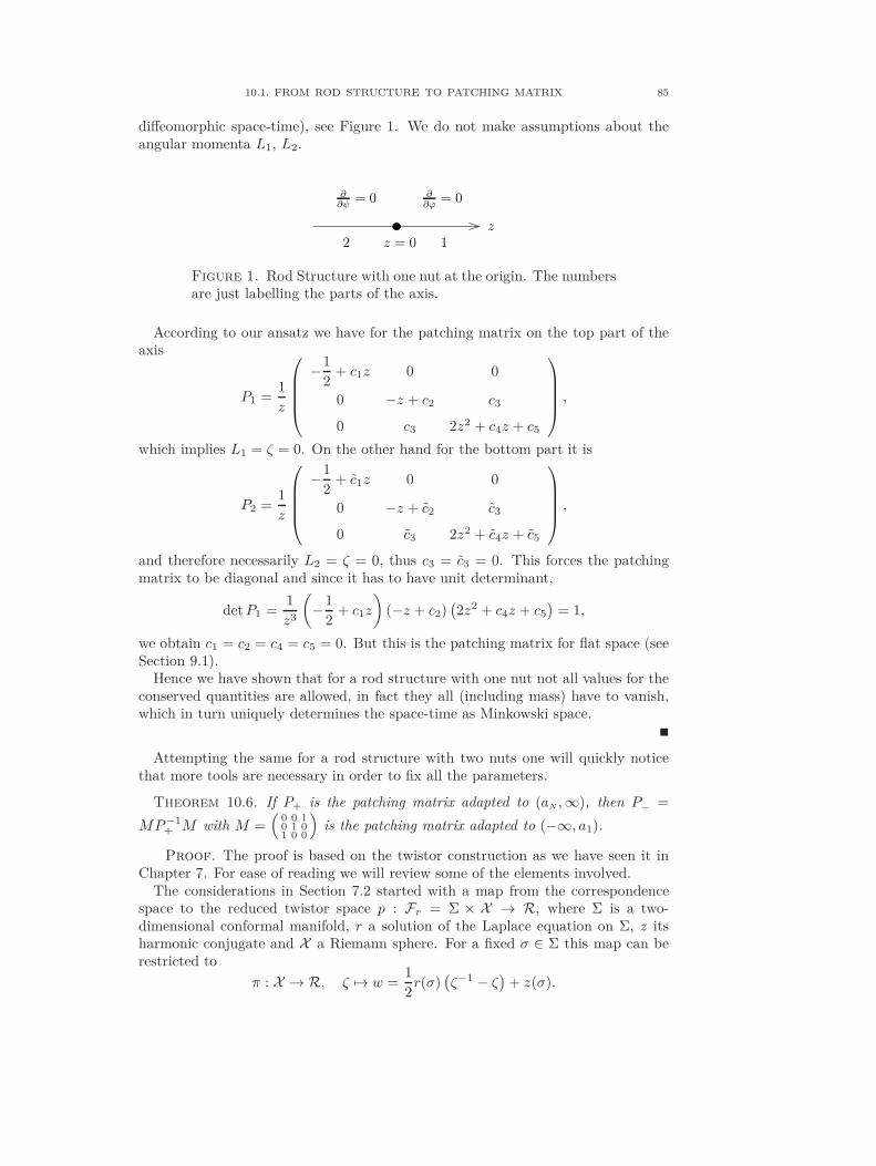
10.1. FROM ROD STRUCTURE TO PATCHING MATRIX 85

diffeomorphic space-time), see Figure 1. We do not make assumptions about theangular momenta L1, L2.

z

∂∂ϕ

= 0

z = 02 1

∂∂ψ

= 0

Figure 1. Rod Structure with one nut at the origin. The numbersare just labelling the parts of the axis.

According to our ansatz we have for the patching matrix on the top part of theaxis

P1 =1

z

−1

2+ c1z 0 0

0 −z + c2 c3

0 c3 2z2 + c4z + c5

,

which implies L1 = ζ = 0. On the other hand for the bottom part it is

P2 =1

z

−1

2+ c1z 0 0

0 −z + c2 c3

0 c3 2z2 + c4z + c5

,

and therefore necessarily L2 = ζ = 0, thus c3 = c3 = 0. This forces the patchingmatrix to be diagonal and since it has to have unit determinant,

detP1 =1

z3

(−1

2+ c1z

)(−z + c2)

(2z2 + c4z + c5

)= 1,

we obtain c1 = c2 = c4 = c5 = 0. But this is the patching matrix for flat space (seeSection 9.1).

Hence we have shown that for a rod structure with one nut not all values for theconserved quantities are allowed, in fact they all (including mass) have to vanish,which in turn uniquely determines the space-time as Minkowski space.

Attempting the same for a rod structure with two nuts one will quickly noticethat more tools are necessary in order to fix all the parameters.

Theorem 10.6. If P+ is the patching matrix adapted to (aN ,∞), then P− =

MP−1+ M with M =

(0 0 10 1 01 0 0

)is the patching matrix adapted to (−∞, a1).

Proof. The proof is based on the twistor construction as we have seen it inChapter 7. For ease of reading we will review some of the elements involved.

The considerations in Section 7.2 started with a map from the correspondencespace to the reduced twistor space p : Fr = Σ × X → R, where Σ is a two-dimensional conformal manifold, r a solution of the Laplace equation on Σ, z itsharmonic conjugate and X a Riemann sphere. For a fixed σ ∈ Σ this map can berestricted to

π : X → R, ζ 7→ w =1

2r(σ)

(ζ−1 − ζ

)+ z(σ).

86 10. THE CONVERSE

Given a bundle E → R one had to assume that π∗(E), the pullback of E to X , istrivial in order to construct J . Then the splitting procedure will provide a J(r, z),which depends smoothly on r and z.

R consists of two Riemann spheres that are identified over a certain set. Therewill always be points, like w = ∞, where the spheres cannot be glued. These pointsare for obvious reasons called double points and the case that is interesting for usis when these points are real and there is only a finite number of them. In otherwords the two spheres are glued together up to the set ∞, a1, . . . , aN.

Therefore, π is only well-defined if one specifies the assignment of these poles tothe spheres. The roots of the double points ai satisfy

rζ2i + 2(ai − z)ζi − r = 0,

so they are

ζ±i =

1

r

((ai − z) ±

√(z − ai)

2 + r2

). (10.1)

We note two things. First, the spheres are labelled by saying that the roots of w =∞, namely ζ = 0 and ζ = ∞, are mapped to π(0) = ∞0 ∈ S0 and π(∞) = ∞1 ∈ S1.Second, r and z are chosen as parameters in the very beginning, but the obtainedexpressions depend smoothly on r and z so that we can vary them and follow theconsequences. One observation of this kind is that for r → 0 one of the roots in(10.1) tends to zero and one to infinity.

Hence, given a solution J of Yang’s equation (5.11) and the corresponding bundleE → RU , U = CP1\∞, a1, . . . , aN the region where the spheres are identified andU not simply connected, then the description of the twistor space as S0 ∪S1 and thepatching matrix P are adapted to the component C of the real axis if those ζ±

i thattend to zero for r → 0 on C are assigned to S0 and those that tend to infinity areassigned to S1; see also [16, Prop. 3.2]. This is merely a requirement of consistentbehaviour under the variation of r and z, since π(0) ∈ S0 and π(∞) ∈ S1. Notethat in this case on C it is P (z) = J ′(z).

More explicitly this can be stated as

ζ+i →

0, i ≤ k

∞, i > kand ζ−

i →

∞, i ≤ k

0, i > k,

for an adaptation to C = (ak, ak+1) and for r → 0 on z ∈ (ak, ak+1).This allows to draw the conclusion that for a given a bundle a change of

adaptation from (ak, ak+1) to (ak−1, ak) is achieved by swapping the assignmentof π(ζ±

k ) to the spheres; see [16, Sec. 3.2]. Following this idea, one then obtainsthe adaptation to (−∞, a1) from an adaptation to (aN ,∞) by swapping all doublepoints π(ζ±

k ), 1 ≤ k ≤ N . However, the latter is the same as swapping the doublepoint at infinity which means relabelling the spheres by saying π(0) ∈ S1 andπ(∞) ∈ S0.

Now let us step back from this line of ideas and have a look from anotherside. Note that if J is a solution of Yang’s equation (5.11) with detJ = 1and J is symmetric, J = J t, then J−1 is a solution of Yang’s equation aswell with detJ−1 = 1. On the other hand, just by inspection of the splittingprocedure one notices that J is defined as a linear map J : E∞0

→ E∞1,

where Ew is the fiber of E → R over w ∈ R, and that J−1 is the solution ofYang’s equation generated by the bundle where the spheres are swapped, S0 ↔ S1


(see also property (3) in [49, Sec. 4]). But this is precisely what we have done above.

The last point to note is that even though we have shown that P−1 is adapted to(−∞, a1) it does not necessarily have to be in our standard form due to the gaugefreedom in the splitting procedure. Using the asymptotic form of P in (9.5) andcomparing the fall-off of P−1 with (9.6) one sees that a flip of the first and thirdrow and column brings P−1 into the desired standard form. This is implementedby the conjugation with M , which completes the proof.

Corollary 10.7. If P+ is the patching matrix adapted to (aN ,∞), then ∆ dividesall 2 × 2-minors of ∆ · P+ = P ′

+.

Proof. From Theorem 10.6 and Proposition 8.18 it follows that P−1+ has at

most simple poles at the nuts. But by the general formula for the inverse of a matrixthe entries of P−1

+ are (up to a sign) P i,j+ /∆2, where P i,j+ is the 2×2-minor of ∆ ·P+

obtained by cancelling the ith row and jth column. Hence one factor of ∆ has tocancel.

This turns out to be a powerful tool as seen in the next example. But before wewould like to point out an implication of the last corollary.

Remark 10.8. Taking the Ernst potential (8.7) in five dimensions and writing itin the following way

J ′+(z) =

g −gχt

−gχ A+ gχχt

=

1

∆

p0 ~p t

~p P

,

the matrix of metric coefficients A as a function of z is obtained as

A =1

∆P− 1

∆p0~p · ~p t =

1

∆p0

(p0P− ~p · ~p t

). (10.2)

All entries of p0P − ~p · ~p t are 2 × 2-minors of ∆ · J ′, hence ∆ divides them. ThusA = P/p0 where the entries of P are polynomials in z. We remember from Section 8.3that p0/∆ blows up when we approach aN , that means p0 cannot have a factor(z − aN ). So, the entries of A are bounded as z ↓ aN , a feature which is consistentwith our picture of space-time.

Note, however, that we cannot extend that to other nuts without changing theadaptation, that is to say, the expression for a metric coefficient Jij(z, r = 0),z > aN , might contain poles for z < aN as the J22 for the black ring shows

J22(z) =

2(z − κ2)(z + cκ2)

z − cκ2, z > κ2,

0 , cκ2 < z < κ2,

2(z − cκ2)(z + cκ2)

z − κ2, −cκ2 < z < cκ2,

0 , z < −cκ2.

The terms in the denominators vanish for certain values of z, but these are not sin-gularities of the metric since they are not in the domain of the respective expression.The reason for pointing out this is that when we try to fix the free parameters in our

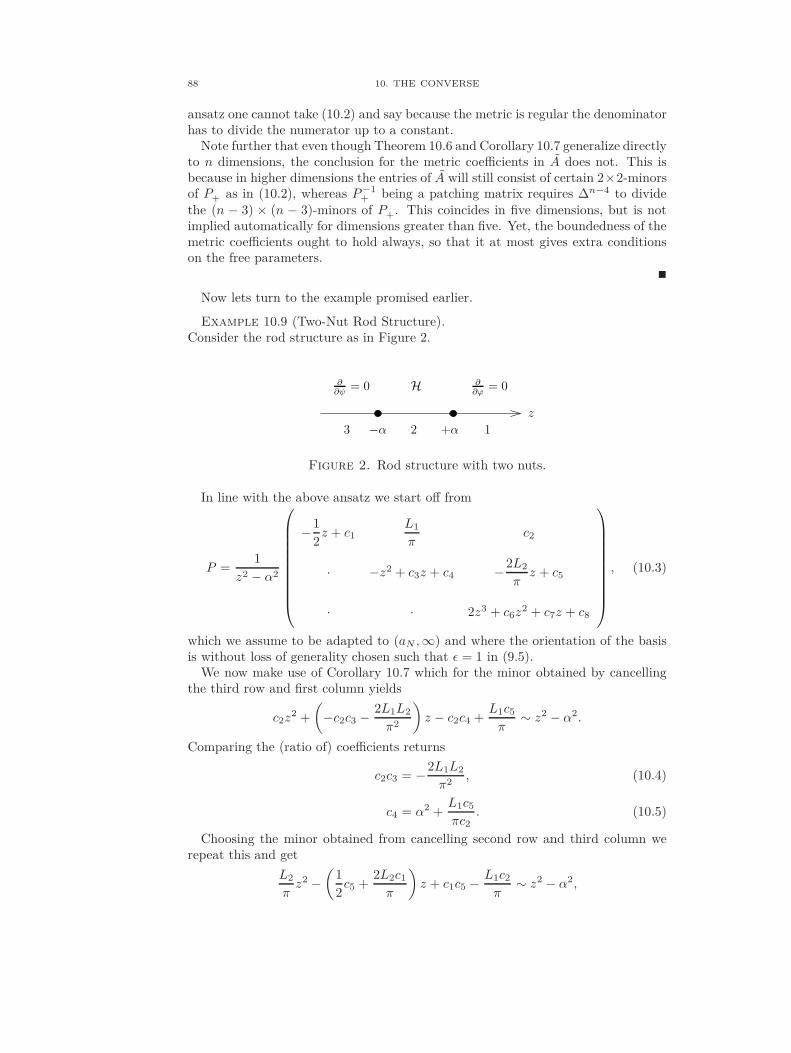
88 10. THE CONVERSE

ansatz one cannot take (10.2) and say because the metric is regular the denominatorhas to divide the numerator up to a constant.

Note further that even though Theorem 10.6 and Corollary 10.7 generalize directlyto n dimensions, the conclusion for the metric coefficients in A does not. This isbecause in higher dimensions the entries of A will still consist of certain 2×2-minorsof P+ as in (10.2), whereas P−1

+ being a patching matrix requires ∆n−4 to dividethe (n − 3) × (n − 3)-minors of P+. This coincides in five dimensions, but is notimplied automatically for dimensions greater than five. Yet, the boundedness of themetric coefficients ought to hold always, so that it at most gives extra conditionson the free parameters.

Now lets turn to the example promised earlier.

Example 10.9 (Two-Nut Rod Structure).Consider the rod structure as in Figure 2.

H∂∂ψ

= 0 ∂∂ϕ

= 0

z

13 +α−α 2

Figure 2. Rod structure with two nuts.

In line with the above ansatz we start off from

P =1

z2 − α2

−1

2z + c1

L1

πc2

· −z2 + c3z + c4 −2L2

πz + c5

· · 2z3 + c6z2 + c7z + c8

, (10.3)

which we assume to be adapted to (aN ,∞) and where the orientation of the basisis without loss of generality chosen such that ǫ = 1 in (9.5).

We now make use of Corollary 10.7 which for the minor obtained by cancellingthe third row and first column yields

c2z2 +

(−c2c3 − 2L1L2

π2

)z − c2c4 +

L1c5

π∼ z2 − α2.

Comparing the (ratio of) coefficients returns

c2c3 = −2L1L2

π2, (10.4)

c4 = α2 +L1c5

πc2. (10.5)

Choosing the minor obtained from cancelling second row and third column werepeat this and get

L2

πz2 −

(1

2c5 +

2L2c1

π

)z + c1c5 − L1c2

π∼ z2 − α2,


thus

c5 = −4L2

πc1, (10.6)

4c21 = α2 − L1

L2c2. (10.7)

These four equations allow us to express c1, c2, c4 and c5 in terms of c3.The coefficients c7 and c8 can be fixed by the minor which results from cancelling

the second row and the first column

−2L1

πz3 +

c6L1

πz2 +

(c7L1

π+

2c2L2

π

)z +

L1c8

π− c2c5 ∼ z3 + bz2 − α2z − bα2,

where b is some constant. Again the ratios of the coefficients for the linear over thecubic and the constant over the quadratic term give

c7 = −2α2 − 2L2

L1c2, (10.8)

c8 = −α2c6 +π

L1c2c5. (10.9)

The last coefficient that remains undetermined is c6, but the determinant is goingto help us for this. The requirement detP = 1 implies

(z2 − α2

)3= z6 +

(1

2c6 − 2c1 − c3

)z5

+

(2c1c3 − c1c6 − c4 − 1

2c3c6 +

1

2c7

)z4 + . . .

The quintic term immediately gives the desired expression

c6 = 4c1 + 2c3. (10.10)

Exploiting furthermore the quartic term we get

−3α2 = 2c1c3 − c1c6 − c4 − 1

2c3c6 +

1

2c7,

which, by using the above obtained relations, is equivalent to

α2 = 4c21 + 4c1c3 + c2

3 +L1

L2c2. (10.11)

Let us relabel the parameters in accordance with [21] as follows

c3 =1

22

0, L1 =π

4a1

20, L2 =

π

4a2

20.

Note that from the asymptotic patching matrix we see that c3 is proportional tothe mass which justifies the implicit assumption about its positiveness in the abovedefinition. However, the parameters (0, a1, a2) are not unconstrained as we willsee soon.

By (10.4) it is

c2 = −1

4a1a2

20. (10.12)

Equations (10.7), (10.11), (10.12) imply

L1

L2c2 = 4c1c3 + c2

3 +L2

L1c2 ⇒ c1 = −1

8

(2

0 + a21 − a2

2

).

90 10. THE CONVERSE

Moreover, from (10.6) and (10.10) we obtain

c5 =1

8a2

20

(2

0 + a21 − a2

2

)and c6 =

1

2

(2

0 − a21 + a2

2

).

Continuing with (10.5) yields

c4 = α2 − 1

82

0

(2

0 + a21 − a2

2

),

so do (10.8) and (10.9) give

c7 = −2α2 +1

2a2

220,

c8 =1

2α2(−2

0 + a21 − a2

2

)− 1

8a2

220

(2

0 + a21 − a2

2

).

With these parameters being determined and with the help of (10.11) we can writeα explicitly as

α2 =1

16

(2

0 − a21 − a2

2

)2 − 1

4a2

1a22. (10.13)

Comparing those expressions with (9.14) one will find that they coincide. However,note that

16α2 = 40 − 22

0

(a2

1 + a22

)+(a2

1 − a22

)2,

which implies that for real non-zero α we need the left hand side to be positive and

therefore 20 >

(|a1| + |a2 |

)2, a condition on the asymptotic quantities familiar from

the discussion of the Myers-Perry solution in [13] and [35], or we need 0 < 20 <(

|a1| − |a2|)2

. This latter possibility is ruled out in [13] and [35] by the additional

requirement that 20 > |a1|2 + |a2|2, and it is also forbidden by [7, Prop. 3.1]. Yet, it

is allowed by our analysis. So, characterizing our solution by the mass and the twoangular momenta we obtain next to the Myers-Perry space-time another branch,which is unphysical.

Mass and angular momenta form a set of three parameters and the position ofthe nuts can be expressed in terms of these three parameters. This is more than onewould have expected by only regarding Theorem 10.3. However, we stated alreadythat by [7, Prop. 3.1] the mass is redundant in the set of parameters. Here we didnot actually eliminate the mass, but the rod length. If one tries vice versa, that isone tries to replace M by α in the set of parameters, then by rearranging (10.13)one is looking for all positive c3 which satisfy a 6th order polynomial. As shownin Appendix J.1, with no further conditions on (α > 0, L1, L2) there are also twopositive solutions for c3 (unless L2

1 = L22 when there is only one). Thus, we are

facing the same problem as before, and this suggests that further conditions needto be imposed on the parameters in order to rule out the unphysical solutions.

Some of the steps above, when we determined all the parameters in the patchingmatrix, only work for L1, L2 , 0. Assuming that one of the angular momentavanishes leads to dichotomies at certain steps when tracing back the parameters.Some of the branches in this tree of possibilities are dead ends others lead to validsolutions such as the Myers-Perry solution with one vanishing angular momentumor an ultrastatic solution, that is where gtt = 1, gti = 0 (but this is not physical asthe mass is zero). On the other hand at no point we used the fact that the middlerod is a horizon.

Note also that issues of conicality cannot arise here as the periodicities of φ, ψare chosen to be 2π on the outer parts of the axis and no further spatial rods are


left. When we turn to higher numbers of nuts more will be required.

Moving on to the next level, that is to a rod structure with three nuts, we willconsider the simpler case where one of the Killing vectors is hypersurface-orthogonal.This simplifies the computation in comparison with the general case as we will.

Example 10.10 (Three-Nut Rod Structure with one Hypersurface-OrthogonalKilling Vector).We consider the rod structure as in Figure 3. Together with L1 = L , 0, L2 = 0

∂∂ϕ

= 0H

3 +α−α +β4 2 1z

∂∂ψ

= 0 ∂∂ψ

= 0

Figure 3. Rod structure with three nuts, where α, β > 0, andS2 × S1 horizon.

this comprises our twistor data. In order to simplify the calculations we would liketo make assumptions such that the two non-diagonal entries in the third row andcolumn of the patching matrix vanish (when adapted to (β,∞)). One thereforeneeds gtψ = gϕψ = 0, however, this cannot be concluded from L2 = 0, as the BlackSaturn shows [8]. The Black Saturn is non-static, but allows vanishing total angularmomentum. We thus make the assumption that ∂ψ is hypersurface-orthogonal, thatis Ψ∧dΨ = 0, and in Appendix K it is shown that this implies χ2 = gtψ = gϕψ = 0.

These assumptions turn our ansatz into

P =1

∆

q(z) l(z) 0

l(z) c(z) 0

0 0 Q(z)

,

where

∆(z) = (z + α)(z − α)(z − β),

q(z) =1

2z2 + c1z + c2,

l(z) =L

πz + c3,

c(z) = −z3 + c4z2 + c5z + c6,

Q(z) = 2z4 + c7z3 + c8z

2 + c9z + c10.

Theorem 10.6 gives the following conditions

qc− l2 = q1∆, q1 quadratic,

Qq = c1∆, c1 cubic,

Ql = q2∆, q2 quadratic,

Qc = Q1∆, Q1 quartic.

(10.14)

92 10. THE CONVERSE

The condition for the patching matrix to have unit determinant then implies

∆3 = Q(qc− l2) = Qq1∆ ⇔ ∆2 = Qq1. (10.15)

Now, as q1 is a quadratic, there are six possibilities for it to be a product of (z+α),

(z−α) and (z−β). But ∂ψ = 0 on (α, β), thus Q∆ → 0 for z ↓ β. To guarantee this

(z−β)2 has to divideQ, which rules out three of those six possibilities. Furthermore,by Theorem 10.6 we have

q1

∆=

1

det A4on (−∞,−α),

where A4 is obtained from J by cancelling the rows and columns containing innerproducts with ∂ψ. But from the general theory we know that the entry of P withthe inverse determinant contains a simple pole when approaching the nut, that isz ↑ −α, so that q1(−α) , 0. This immediately yields

q1 =1

2(z − α)2 and by (10.15) also Q = 2(z + α)2(z − β)2.

Now observe that there is a factor of (z − α) in ∆ but not in Q, so that by (10.14)the monic (z − α) has to divide l, q and c. We write this as

l =L

π(z − α), q = −1

2(z − α) l1, c = −(z − α) q3,

where

l1 = z +A, q3 = z2 +Bz + C for A,B,C = const.

The first equation in (10.14) then turns into

l1q3 − 2L2

π2= ∆

⇔ z3 + (A+B)z2 + (C +AB)z +AC − 2L2

π2= z3 − βz2 − α2z + α2β.

Comparing the coefficients one sees

B = −A− β, C +AB = −α2, AC − 2L2

π2= α2β,

and therefore A satisfies

1

A

(α2β +

2L2

π2

)−A(A+ β) = −α2

⇔ A3 + βA2 − α2A− α2β − 2L2

π2= 0.

Writing F (a) ≔ a3 + βa2 − α2a− α2β − 2L2

π2, we see that since F (0) < 0, this last

polynomial has to have at least one (positive) real root (see Figure 4). Now fromF ′(A) = 3A2 + 2βA− α2 one concludes that the local maximum of F is at

amax = −1

3

(β +

√β2 + 3α2

).

Furthermore, note that since α ≤ β, it is

amax ≤ −1

3

(α+

√α2 + 3α2

)= −α and

F (−α) = −2L2

π2< 0,


F (a)

aAamin−αamax

Figure 4. The cubic F (a).

which implies that if F has two more real roots, they will both be smaller than −α.On the other hand there is a constraint on A obtained from the asymptotics. Inour patching matrix the central entry is

c

∆= − (z − α)(z2 +Bz + C)

∆= −1 + (α− β −B)z−1 + . . .

Using (9.5) and the relation between A and B, this gives

A+ α =4M

3π.

Positivity of M thus implies A > −α and we therefore have shown that there is aunique positive A ∈ R which satisfies all the constraints.

Consequently, by our ansatz we are able to fix all the parameters in terms of α,β, L, that is in terms of the given data, and the patching matrix is

P1 =

− z +A

2(z + α)(z − β)

L

π(z + α)(z − β)0

· − z2 − γz + δ

(z + α)(z − β)0

0 02(z + α)(z − β)

z − α

,

whereγ = β +A, δ = −α2 + βA+A2.

Note that λ and A are zeros of the same polynomial and are restricted by the sameinequality involving the mass, so this is the patching matrix for the black ring withthe conical singularity not fixed, see (9.19).2 For the regular black ring the angular

2I am grateful to Harvey Reall for suggesting this possibility, which turns out to be correct.

94 10. THE CONVERSE

momentum can also be expressed in terms of α and β. We will see in Section 10.5how this can be done in the twistor picture.

10.2. Local Behaviour of J around a Nut

For the general case of a rod structure with three nuts and especially as the numberof nuts gets higher, one will find it increasingly difficult to reduce the number of freeparameters to a minimum and would therefore like to obtain more constraints fromthe inner rods. With this desire in mind it would be useful to have an understandingof how the patching matrices with adaptations to adjacent rods are related to eachother. We have seen an example in Theorem 10.6, which can be considered as sucha switch at the nut at infinity. The proof gives an idea of what is happening whenchanging the adaptation, yet it will be more difficult for interior nuts, that is nutsfor which |ai| is finite.

A strategy of how to achieve this is describred in Fletcher [16, Ch. 3]. Therethe essence is that “... redefining the sphere S0 and S1 by interchanging doublepoints alters the part of the real axis to which the bundle is adapted.” [16, Sec. 3.2].However, as the example in [16, Sec. 5.1] shows, this comes down to a Riemann-Hilbert problem which will be rather hard and impractical to solve in five or evenhigher dimensions. Thus we will approach this task in a different way. The ideais that we start off as above on the outermost rods where |z| → ∞, determine asmany free parameters as possible by the constraints which we have got on theserods, then take the resulting P -matrix (still having free parameters in it which wewould like to pin down), calculate its adaptation to the next neighbouring rod andapply analogous constraints there. But before looking at the patching matrix itselflet us first study how J behaves locally around a nut.

Consider first a nut where two spatial rods meet, that is like in Figure 5.

∂∂ψ

= 0 ∂∂ϕ

= 0

z

u = 0v = 0

Figure 5. Two spatial rods with their rod vectors meeting at a nut.

Without loss of generality assume that the nut is at z = 0. In this case a suitablechoice of coordinates are the (u, v)-coordinates defined as

r = uv, z =1

2(v2 − u2) ⇔ u2 = −z ±

√r2 + z2, v2 = z ±

√r2 + z2,

where the signs on the right-hand side are either both plus or both minus. If wechoose both signs to be plus, then the rod ∂ϕ = 0 corresponds to u = 0 and ∂ψ tov = 0. The metric in the most general case has the form

ds2 = X dt2 + 2Y dtdϕ+ 2Z dtdψ + U dϕ2 + 2V dϕdψ +W dψ2

+ e2ν(u2 + v2)(du2 + dv2),(10.16)

10.2. LOCAL BEHAVIOUR OF J AROUND A NUT 95

or equivalently

J(u, v) =

X Y Z

· U V

· · W

.

We assume that φ, ψ have period 2π.

Theorem 10.11. For a space-time regular on the axis the generic form of J in(u, v)-coordinates around a nut, where two spacelike rods meet, is

J =

X0 u2Y0 v2Z0

· u2U0 u2v2V0

· · v2W0

, (10.17)

and, furthermore, one needs

• U0

v2e2ν= 1 as a function of v on u = 0,

• W0


If one of the rods is the horizon instead of a spacelike rod corresponding statementshold.

The second part of the theorem is closely tied to the problem of conicality, whichwe will investigate shortly.

Proof. Introduce Cartesian coordinates

x = u cosφ, y = u sinφ, z = v cosψ, w = v sinψ, (10.18)

then the metric becomes in these coordinates

ds2 = X dt2 + 2Y

u2dt(xdy − y dx) + 2

Z

v2dt(z dw − w dz) +

U

u4(xdy − y dx)2

+ 2V

u2v2(xdy − y dx)(z dw − w dz) +

W

v4(z dw − w dz)2

+ e2ν(u2 + v2)

(1

u2(xdx+ y dy)2 +

1

v2(z dz + w dw)2

).

(10.19)

The x, y, z, w are not to be confused with the earlier use of the same symbols. SetX0 = X . Now as u → 0 for constant v we immediately see that in order for gtyand gxw to be bounded we need Y = u2Y0 and V = u2V1 for bounded Y0, V1.3 Theremaining singular terms are

U

u4(xdy − y dx)2 + e2ν(u2 + v2)

1

u2(xdx + y dy)2.

For the fourth-order pole not to be dominant we need U = u2U0 for bounded U0;then it is required

U0

v2e2ν= 1 as a function of v on u = 0 (10.20)

to remove the remaining second-order pole.

3Remember that for polar coordinates (u, φ) the angle φ is bounded in the limit to but notcontinuous (or even differentiable) at the origin u = 0. Thus x

uis not bounded towards the origin.

96 10. THE CONVERSE

Repeating this for v → 0 with fixed u yields Z = v2Z0, V1 = v2V0, W = v2W0

andW0


This is the minimum that we can demand in terms of regularity of J on the axisand near the nuts.

Assuming now without loss of generality that in Figure 5 the axis segment wherev = 0 is the horizon, we have seen in Chapter 8 that then the first row and firstcolumn degenerate. So, we substitute

z = v cosh(ωt), w = v sinh(ωt),

where ω is a constant with no further restriction. The coordinates x and y choose asin (10.18). Now the above argument works analogously with all results equivalent,but

X0

v2e2ν= −ω2 as a function of v on u = 0.

10.3. Conicality and the Conformal Factor

Returning to the case as depicted in Figure 5, we saw in (10.20) that regularity atan axis seqment where ∂φ vanishes forces a relation between gφφ and the conformalfactor e2ν of the (r, z)-metric. In this section we first establish the following.

Proposition 10.12. On a segment of the axis where u = 0 we have U0

v2e2ν =constant.

Proof. To prove this we need to consider how the conformal factor varies onthe axis and this is obtained from (5.19) which we may write as

∂ξ(log(re2ν

))=

ir

2tr(J−1JξJ

−1Jξ). (10.21)

It will be convenient to work with χ = u+iv where ξ = z+ir = 12χ

2 and concentrate

on the conformal factor of the (u, v)-metric which is (u2 + v2)e2ν by (10.19). Then

∂χ(log((u2 + v2

)e2ν))

= ∂χ(log((u2 + v2

)(uv)−1re2ν

))

=1

χ− 1

2u+

i

2v+

iuv

2(u+ iv)tr(J−1JχJ

−1Jχ).

Close to the axis segment u = 0 we substitute from (10.17) and expand in powersof u to find

∂χ(log((u2 + v2)e2ν

)))=

1

χ− 1

2u+

i

2v+

iuv

2(u+ iv)

(K1

u2+K2

u+ O(1)

), (10.22)

where

K1 =(U0

(X0W0 − v2Z2

0

))2= 1 +

1

v2O(u2),

K2 =(U0

(X0W0 − v2Z2

0

))2 ∂χU0

U0.

The right hand side of the first equation follows from the determinant

u2v2 = detJ = u2v2X0U0W0 − u2v4U0Z20 + O

(u4),

10.3. CONICALITY AND THE CONFORMAL FACTOR 97

hence

1 = U0

(X0W0 − v2Z2

0

)+

1

v2O(u2).

Taking in (10.22) the limit on to u = 0 we obtain just

∂v(log(v2e2ν

))= ∂v log (U0) ,

so thatU0

v2e2ν= constant on u = 0.

Thus (10.20) will hold at all points of the axis segment if it holds at one. Thefollowing proposition is an analysis similar to [21, App. H], but it is simpler andmore self-contained to rederive it than translate it.

Proposition 10.13. As a function on the axis u = 0 ∪ v = 0, that is as afunction of one variable, the factor

(u2 + v2

)e2ν is continuous at the nut u = v = 0.

Proof. Near the nut introduce polar coordinates

u = R cos Θ, v = R sin Θ,

so that from (10.21) and with the help of

uv∂z = v∂u − u∂v, uv∂r = u∂u + v∂v, ∂ξ =1

2(∂z − i∂r)

we get

∂Θ

(log((u2 + v2

)e2ν))

= (u∂v − v∂u)(log((u2 + v2

)e2ν))

= (u∂v − v∂u)

(log

(u2 + v2

uv

))− r∂z

(log(re2ν

))

= −u

v+v

u− (uv)2

4tr(J−1JzJ

−1Jr)

= −u

v+v

u− uv

4tr(J−1JuJ

−1Ju − J−1JvJ−1Jv

).

Again we expand this using (10.17) to find

∂Θ

(log((u2 + v2

)e2ν))

= −u

v+v

u− v

u

(U0

(X0W0 − v2Z2

0

))2

+u

v

(W0

(X0U0 − u2Y 2

0

))2+ O(u) + O(v)

= O(u) + O(v) = O(R).

Now the jump in log(u2 + v2

)e2ν round the nut is

∆(log((u2 + v2

)e2ν))

= limR→0

∫ π2

0∂Θ

(log((u2 + v2

)e2ν))

dΘ = 0,

and(u2 + v2

)e2ν does not jump either.

On u = 0, U0 is continuous and by Proposition 10.12 U0

v2e2ν = constant, so v2e2ν

must be bounded there. Similarly, on v = 0 for W0 and W0

u2e2ν . Thus,(u2 + v2

)e2ν

is continuous on the two rods and has no jump across the nut, so it is continuouson the axis.

98 10. THE CONVERSE

The strategy for removing conical sigularities is now clear: We start by assumingthat φ and ψ both have period 2π. On the part of the axis extending to z = +∞,where the Killing vector ∂φ vanishes, we have U0

v2e2ν = constant by Proposition 10.12and the asymptotic conditions we are imposing make this constant one. The corre-sponding statement holds on the part of the axis extending to z = −∞ for the samereason. When passing by a nut between two spacelike rods we may suppose, bychoosing the basis of Killing vectors appropriately, that ∂φ vanishes above the nutand ∂ψ below and we know by Proposition 10.13 that

(u2 + v2

)e2ν is continuous

at the nut. If there is no conical singularity above the nut we have U0

v2e2ν = 1 there

and we want W0

u2e2ν = 1 below the nut. Therefore we require the limits of U0 fromabove and W0 from below to be equal.

Corollary 10.14. With the conventions leading to (10.17), the absence of con-ical singularities requires

limv→0

U0 = limu→0

W0.

This is what we have just shown. At a nut where one rod is the horizon we do notobtain further conditions as we have no reason to favour a particular value of ω. Tosee how this is applied to the case of the black ring we need a better understandingof going past a nut.

10.4. Local Behaviour of P around a Nut: Switching

In this section we establish a prescription for obtaining the matrix P− adapted to thesegment of the axis below a nut from the matrix P+ adapted to the segment above.We call this process ‘switching’. Once we have the prescription we can imposethe condition of non-conicality found in Corollary 10.14. We then apply this tothe black ring, but it is clear that with this prescription we have an algorithm forworking systematically down the axis given any rod structure so that we obtainall the matrices Pi adapted to the different rods labelled by i. The result is thefollowing.

Theorem 10.15. Let at z = a be a nut where two spacelike rods meet, as inFigure 5, and assume that we have chosen a gauge where the twist potentials vanishwhen approaching the nut. Then

P− =

0 01

2(z − a)

0 1 0

2(z − a) 0 0

P+

0 0 2(z − a)

0 1 01

2(z − a)0 0

,

where P+ is adapted to u = 0 and P− is adapted to v = 0.

We begin by motivating this prescription from a consideration of (10.16). Firstcalculate the twist potentials in the same way as in Chapter 9. The metric (10.16)can be rearranged in orthonormal form

ds2 = X(dt+ ω1 dϕ+ ω2 dψ)2 + U(dϕ+ Ω dψ)2

+ W dψ2 − e2ν(dr2 + dz2).

10.4. LOCAL BEHAVIOUR OF P AROUND A NUT: SWITCHING 99

The orthonormal frame is again

θ0 = X12 (dt+ ω1 dϕ+ ω2 dψ), θ1 = U

12 (dϕ + Ω dψ),

θ2 = W12 dψ, θ3 = eν dr, θ4 = eν dz,

so

Xω1 = Y, Xω2 = Z Xω1ω2 + UΩ = V,

U +Xω21 = U, W + UΩ2 +Xω2

2 = W.

Adapted to ∂ψ = 0, then for small r it is Z, V,W ∈ O(r2), hence ω2,Ω, W ∈ O(r2),4

and the other terms O(1). This implies WW

→ 1 as r → 0.Now the 1-forms are

∂t → T = X12 θ0, ∂ϕ → Φ = ω1X

12 θ0 + U

12 θ1,

hence

dχ1 = ∗(T ∧ Φ ∧ dT ) = ∗(X12 θ0 ∧ U

12 θ1 ∧X dω2 ∧ dψ)

dχ2 = ∗(T ∧ Φ ∧ dΦ) = ∗(X12 θ0 ∧ U

12 θ1 ∧ (ω1X dω2 + U dΩ) ∧ dψ),

which with ∗(θ0 ∧ θ1 ∧ θ2 ∧ θ3) = ǫθ4 leads to

∂zχ1 = ǫ(XU)12X lim

r→0

(∂rω2

W 1/2

)

∂zχ2 = ǫ(XU)12 limr→0

(Xω1∂rω2 + U∂rΩ

W 1/2

).

We switch again to (u, v)-coordinates by using

∂

∂u= u

∂

∂z+ v

∂

∂r,

∂

∂v= −v ∂

∂z+ u

∂

∂r.

On v = 0 this yields

∂χ1

∂u= u

∂ψ1

∂z= uǫ(XU)

12X lim

v→0

(1

uW 1/2

∂ω2

∂v

).

Now use5

ω2 =Z

X=v2Z0

X0and W = v2W0 + O(v4),

4In order to see that Ω ∈ O(r2), derive from X ∈ O(1) and UX = UX − Y 2 that U ∈ O(1).5NB: If we did not have Z = v2Z0 already, then we could impose it here without loss of generality,since a smooth metric invokes smooth twist 1-forms, but χ1 becomes singular for v → 0 if onlyZ = vZ0.

100 10. THE CONVERSE

to obtain

∂χ1

∂u= ǫ

(X0U

) 12

2vZ0

vW 1/2

0

= 2ǫ

(X0U

) 12 Z0

W 1/2

0

= 2ǫZ0

W 1/2

0

(u2U0X0 − u4Y 2

0

) 12

= 2ǫZ0

(U0X0

W0

) 12

u+ O(u2)

⇒ χ1 = χ01 + χ1

1u2 + h.o.

Analogous steps lead to

∂χ2

∂u= u

∂χ2

∂z= uǫ(XU)

12 limv→0

u2Y0

1u∂ω2

∂v+(U − Y 2

X

)1u∂vΩ

vW 1/2

0

= 2u2(XU)12

Y0Z0

X0W1/2

0

+

(U0 − Y 2

0

X0

)1u

Ω0,v

vW 1/2

0

= 2ǫV0

(U0X0

W0

) 12

u3 + h.o.

⇒ χ2 = χ02 + χ1

2u4 + h.o.

For u = 0 we only have to swap Y ↔ Z, U ↔ W . With u2 ∼ 2z the above can besummarized as

P−(r = 0, z) =

g0

2z+ O(1) −g0χ

11 + O(z) −g0χ

12z + O(z2)

· X0 + O(z) 2zY0 + O(z3)

· · 2zU0 + O(z4)

,

where g0 = (X0U0 −2zY 20 )−1. Note that here we dropped without loss of generality

the constant terms of the twist potentials χ0i . This can be done just by a gauge

transformation to P of the form P → APB with constant matrices A and B, namely

P →

1 0 0

−c1 1 0

−c2 0 1

P

1 −c1 −c2

0 1 0

0 0 1

.

For P in standard form this results in χi → χi+ ci. Removing the constant term inthe twist potentials allows us to assume that without loss of generality the entrieswhich become zero or blow up towards a nut are only on the diagonal. The off-diagonal entries are bounded towards the nut.

Without loss of generality assume that the nut is at a = 0. Then the calculationsabove show that to leading order in z the patching matrices below and above the

10.4. LOCAL BEHAVIOUR OF P AROUND A NUT: SWITCHING 101

nut are6

P− =

1

2zX0U0− Z0

(U0X0W0)1/2− V0z

(U0X0W0)1/2

· X0 2zY0

· · 2zU0

, (10.23)

P+ =

− 1

2zX0W0

Y0

(U0X0W0)1/2− V0z

(U0X0W0)1/2

· X0 −2zZ0

· · −2zW0

. (10.24)

Using that det J = −u2v2 in (10.17) and thus X0U0W0 = −1 to leading order in zwe see that the switching is correct to leading order in z. (This is consistent withthe different adaptations we calculated for example for the Schwarzschild space-timeor flat space, see Section 9.4.)

Proof of Theorem 10.15. To prove Theorem 10.15 the strategy is to followthe splitting procedure outlined in Section 8.4.

We first observe that splitting P+ as in (10.23) will lead not to J(r, z) as desired,but to J(r, z) with its rows and columns permuted. This can be seen by looking atthe diagonal case. To obtain J(r, z) with the rows and columns in the order (t, φ, ψ)we need to permute

P+ → P+ = E1P+E1 with E1 =

0 1 01 0 00 0 1

.

Similarly for P− by (10.24), we permute

P− → P− = E2P−Et2 with E2 =

0 1 00 0 11 0 0

.

Note that now the prescription in Theorem 10.15 translates to

P− = DP+D with D =

1 0 0

0 2z 0

0 01

2z

. (10.25)

6Chosen the right orientation for the basis such that the signs which are recorded by ǫ work out.


Recall that we have set a = 0. Following Chapter 8, to obtain J we split thematrices

P+ =

1 0 0

0r

ζ0

0 0 1

P+

1 0 0

0 −rζ 0

0 0 1

,

P− =

1 0 0

0 1 0

0 0r

ζ

P−

1 0 0

0 1 0

0 0 −rζ

.

(10.26)

The location of the diagonal entries which are not one is dictated by the position ofthe Killing vector which vanishes on the section of axis under consideration withinthe basis of Killing vectors (∂t, ∂φ, ∂ψ) . In the language of Section 8.4, the integers(p0, p1, p2) are, as we know, a permutation of (0, 0, 1) and the location of the 1 isdetermined by the prescription just given.

Assembling (10.25) and (10.26) to

P− = AP+B,

where

A =

1 0 0

02zζ

r0

0 0r

2zζ

, B =

1 0 0

0 −2z

rζ0

0 0 − rζ

2z

,

all that is needed for completing the proof is to show that splitting the left and righthand side of this last equation yield the same J-matrix. To perform the splitting,we replace all appearances of z by w and make the substitution (7.14). Note that

w = z +r

2

(ζ−1 − ζ

)=

1

2

(u2 − v2 + uv

(ζ−1 − ζ

))=

1

2ζ(uζ + v) (u− vζ) ,

so that

2wζ

r=

(uζ + v)(u − vζ)

uv= 1 +O (ζ) ,

−2w

rζ= − 1

ζ2

(uζ + v)(u − vζ)

uv= 1 +O

(ζ−1

).

Thus A(z, r, ζ) is holomorphic and nonsingular in the neighbourhood of ζ = 0 withA(z, r, 0) = id, and B(z, r, ζ−1) is holomorphic and nonsingular in the neighbour-

hood of ζ−1 = 0 with B(z, r, 0) = id. Consequently, if P+ splits as

P+ = K0+ (r, z, ζ)

(K∞

+

(r, z, ζ−1

))−1,

with K0+ holomorphic and nonsingular in the neighbourhood of ζ = 0 and K∞

+

holomorphic and nonsingular in the neighbourhood of ζ−1 = 0, then a splitting of

P− is given by taking

P− = K0−(K∞

−)−1

with K0− = AK0

+, K∞− = B−1K∞

+ .

10.5. APPLICATION TO THE BLACK RING 103

The corresponding expressions for J are

J = J+(r, z) = K0+(0)

(K∞

+ (0))−1

and

J = J−(r, z) = K0−(0)

(K∞

− (0))−1

= A(r, z, 0)J+(r, z)B(r, z, 0) = J+(r, z).

These are the same.

10.5. Application to the Black Ring

Now we see how to apply the prescription for switching and the discussion of con-icality to P (z) for the black ring as in (9.19). We are interested in the nut withlargest z-value, which is the one at z = β. The first step is to make an additiveshift to the twist potential χ to ensure that the term P12 in (9.19) is finite at z = β.This needs

χ → χ+ C, C = − 2ν

β + λ,

when

P12 → P12 − CP11 = P12 − ν(z + λ)

(β + λ)(z + α)(z − β)=

ν

(z + α)(β + λ),

which is indeed finite at z = β, and

P22 → P22 − 2CP12 + C2P11 = − (z + µ)

(z + α), where µ =

κ2(2b− c+ bc)

(1 + b),

which is also finite at z = β. We are in position to make the switch as in Theo-rem 10.15 with β in place of a and the result is

P2 =

(z + α)

2(z − α)(z − β)0 0

· − (z + µ)

(z + α)

2ν(z − β)

γ(z + α)

· · −2(z + λ)(z − β)

(z + α)

.

We have completed the switching and obtained P2(z), the transition matrix adaptedto the section of axis α < z < β. We could continue to find the transition matrixadapted to the other segments but that is straightforward and we do not need it.Instead we shall return to the question of conicality addressed in Corollary 10.14.Compare with Theorem 10.11 to find from P1 that

v2W0 =2(z + α)(z − β)

(z − α)

where now v2 = −2(z − β) and from P2 that

u2U0 = −2(z + λ)(z − β)

(z + α)

where now u2 = 2(z−β). Corollary 10.14 implies that there is no conical singularityon the axis section α < z < β provided

limu→0

W0 = limv→0

U0,


which here requiresβ + λ

β + α=β + α

β − α.

Using (9.20) this condition can be solved for b as

b =2c

1 + c2

which is known [10] (or [21, Eq. (6.20)]) to be the right condition.

CHAPTER 11

Summary and Outlook

In this work we have presented a possible way for the reconstruction of five- orhigher-dimensional black hole space-times from what are at the moment believed tobe the classifying parameters, rod structure and angular momenta. The method isbased on a twistor construction which in turn relies on the Penrose-Ward transform.

Our idea assigns a patching matrix to every rod structure where, apart from thepossible poles at the nuts, the entries of the patching matrix have to be rationalfunctions with the same denominator ∆ — Chapter 10. By imposing boundaryconditions the aim is to determine all the coefficients of the polynomials in thenumerator of these rational functions in terms of the nuts and angular momenta.

However, with an increasing number of nuts one needs increasingly sophisticatedtools and it is of particular importance to gain a detailed understanding of how thepatching matrices, adapted to two neighbouring rods, are related. In Theorem 10.15we show how to do this and Theorem 10.6 provides this statement for the nut atinfinity, that is, it relates the patching matrices which are adapted to the outer rods.By means of that we are able to reconstruct the patching matrix for a general two-nut rod structure (up to one restriction on the parameters for the physical Myers-Perry solution) and we can show that a three-nut rod structure with one Killingvector hypersurface-orthogonal fixes, together with a given angular momentum, thespace-time to be the black ring.

Also in Chapter 10 we discuss conical singularities on the axis and show how toobtain necessary and sufficient conditions for their removal. Applying this to theblack ring we obtain the known relation between the parameters. In particular,this implies a relation between the rod structure and the asymptotic quantities fora non-singular solution known to exist.

Further questions which are interesting to pursue in this context are for example:Which rod structures are admissible? In other words, are there any restrictions

on the rod structures which one allows in the set of parameters?Can we construct a Lens space-time this way, that is a space-time whose horizon

is connected and has the topology of a Lens space [24, Prop. 2]? We know what thecorresponding rod structure looks like, but are we able to fix enough parametersand can we see whether the resulting patching matrix does give rise to a space-time without singularities? The latter question seems to be difficult to address asby the analytic continuation one can guarantee the existence of the solution withall its nice regularity properties only in a neighbourhood of the axis, but furtheraway from the axis there might be so-called “jumping lines”, where the mentionedtriviality assumption of the bundle does not hold.

How many dimensions does the moduli space for an n -nut rod structure have?Can we find upper and lower bounds on that depending on the imposed boundary

105

106 11. SUMMARY AND OUTLOOK

conditions? This also does not seem to be an easy questions as most of the con-ditions we impose on the patching matrix are highly non-linear, for example thedeterminant condition.

Which parts of the theory extend to higher dimensions? We have already pointedout along the way that some statements straight-forwardly generalize to more thanfive dimensions as well, but some others do not. A closer look at those points iscertainly interesting.

Also stepping a dimension down leads to a question for which this set of toolsmight be appropriate. Are we able to disprove the existence of a double-Kerr solu-tion in four dimensions? It is conceivable that for example the imposed compatibilityrequirements as one switches at the nuts lead finally to an overdetermined systemof conditions and thereby provoke a contradiction.

Appendix

A. Conformal Metrics and Null Separated Points

We show that two symmetric (0,2)-tensors are conformally equivalent if and onlyif their sets of null vectors are identical (assuming that we have a bijection or adiffeomorphism between the underlying manifolds). If the (pseudo-) metrics areconformally equivalent, then the null vectors are obviously identical. Conversely,if we know that the (pseudo-) metrics g1, g2 leave the null cones invariant, thentimelike or spacelike vectors, respectively, in g1 correspond to timelike or spacelikevectors, respectively, in g2. We are interested in the Lorentzian case, and choose anorthonormal tetrad e0, e1, e2, e3 for g1 such that e0 is timelike and e1, e2, e3 arespacelike. By the assumption that null cones are preserved this is also orthogonaltetrad for g2, and

g1(e0, e0) = 1 ⇒ g2(e0, e0) = λ > 0,

g1(ei, ei) = 1 ⇒ g2(ei, ei) = µi < 0, i = 1, 2, 3.

Moreover, e0 + ei is null for g1 hence for g2

0 = g2(e0 + ei, e0 + ei) = g2(e0, e0) + 2g2(e0, ei) + g2(ei, ei)

= g2(e0, e0) + g2(ei, ei) = λ− µi.

This shows that all nonzero coefficients for g2 are the same, that is g1 and g2 areconformally equivalent.

B. Characterization of Simple Bivectors

A bivector xαβ is simple ⇔ εαβγδxαβxγδ = 0 ⇔ ∗xαβxαβ = 0.

Proof. xαβ is simple ⇒ εαβγδxαβxγδ = 0:

εαβγδxαβxγδ = εαβγδ(Z

αZβ − ZβZα)(ZγZδ − ZδZγ)

= εαβγδ(ZαZγZβZδ − ZαZδZβZγ

− ZβZγZαZδ + ZβZδZαZγ)

= 4ǫαβγδZαZγZβZδ

= 0.

εαβγδxαβxγδ = 0 ⇒ ∗xαβxαβ = 0 : ∗xαβxαβ =

1

2∆ǫαβγδx

γδxαβ = 0

∗xαβxαβ = 0 ⇒ xαβ is simple: First note that xαβ has to have rank 0, 2 or 4,because it is skew-symmetric (its non-degenerate part defines a symplectic bilinearform and symplectic vector spaces are even-dimensional). This implies that if x

107

108 APPENDIX

has an eigenvector with eigenvalue 0, then x has to be of rank 2 or 0. Supposingthat xαβ is nonzero we can set 2 rows and 2 columns zero. But then x has to be ofthe form xαβ = Z [αZβ]. It remains to show that such an eigenvector exists. Usingrelations for the alternating symbol one can verify that

yαγxβγ − ∗xαγ ∗ yβγ =1

2xδλyδλδ

αβ

for bivectors xαβ , yαβ. Setting yαβ = ∗xαβ and using ∗2 = 1, ∆2 = −1 yieldsimmediately

∗xαβxβγ = 0 ⇐⇒ ∗xαβxαβ = 0.

So, our assumption implies that xβγqγ is an eigenvector with eigenvalue 0 for anarbitrary qγ .

C. Computation for Reduced Einstein Equations

Using (5.15) and the Ricci identity we obtain

RabXai X

bj = Xb

jRcacbX

ai = −Xb

j∇c∇cXib

= −1

2Xbj∇c

(J lk((∂cJik)Xlb − (∂bJki)X

cl )).

Expanding by Leibniz rule

RabXai X

bj = −1

2(∇cJ

lk) · (XbjXlb︸︷︷︸

=Jjl

(∂cJik) −Xbj (∂bJki)︸︷︷︸

=0

Xcl )

− 1

2XbjXlb︸︷︷︸

=Jjl

J lk∇c∂cJik − 1

2J lk(∂cJik)Xb

j∇cXlb︸︷︷︸12∂cJjl

+1

2J lkXc

lXbj∇c∂bJki +

1

2JklXb

j (∂bJki)︸︷︷︸=0

∇cXcl ,

and using (5.14) together with the expression for the Laplace-Beltrami operator

l u = ∇a∇au =1√|g|∂a

(√|g|gab∂bu

),

this yields

RabXai X

bj = −1

2Jjl(∂

cJik)(∂cJlk) − 1

2l Jij − 1

4J lk(∂cJik)(∂cJjl)

+1

2J lkXc

l ∇c(Xbj∂bJki︸︷︷︸

=0

) − 1

2J lkXc

l ∇c(Xbj )︸︷︷︸

− 12∂bJjl

∂bJki.

Some further substitutions and cancellations lead to

RabXai X

bj = −1

2Jjl(∂


2l Jij

− 1

4J lk(∂cJik)(∂cJjl) +

1

4J lk(∂cJik)(∂cJjl),

E. INTEGRABILITY OF EINSTEIN EQUATIONS 109

and eventually

RabXai X

bj = −1

2Jjl(∂


2l Jij

= −1

2JikJ

kll Jlj − 1

2Jjkg

− 12 (∂aJ

kl)g12 gab(∂bJli)

= −1

2Jikg

− 12 ∂a(g

12 gabJkl∂bJlj)

as claimed. Note that the covariant derivative for the functions Jik is the same asthe partial derivative.

D. Isothermal Coordinates

Isothermal coordinates on a manifold are local coordinates where the metric has theform

ds2 = e2ν(dx21 + . . . dx2

n)

with eν a smooth function. In the real case the manifold should be Riemannian sothat isothermal coordinates are conformal to the Euclidean metric.

For a 2-surface isothermal coordinates always exist locally, which can be seen asfollows. The coordinates r and x are isothermal if they satisfy

∗dr = dx

where ∗ is again the Hodge star operator. Suppose ∆ = dδ+δd = δd is the Laplace-Beltrami operator on functions,1 then by standard elliptic theory, we can choose rto be harmonic near a given point, that is ∆r = 0, with non-vanishing gradientdr. In our case we were given such an r. By the Poincaré lemma ∗dr = dx has alocal solution x if and only if d ∗ dr = 0. Because of δ = ∗d∗, this is equivalent to∆r = 0, thus local solutions exists. From the facts that dr is non-zero and ∗2 = −1on 1-forms, we conclude that dr and dx are necessarily linearly independent, andtherefore give local isothermal coordinates.

In our case the overall sign of the metric is not fixed, because we only asked theorthogonal 2-surfaces to be non-null. But the exclusion of null vectors still leavestwo possibilities for the signature, (+,+) or (−,−).

E. Integrability of Einstein Equations

The second part of the reduced vacuum Einstein equations (5.19) are in full

2i∂ξ(log re2ν) = r tr(∂ξJ−1∂ξJ),

−2i∂ξ(log re2ν) = r tr(∂ξJ−1∂ξJ).

By use of (5.11) and the constraint detJ = −r2, we have to show that they areintegrable, that is

∂ξ∂ξ(log re2ν) = ∂ξ∂ξ(log re2ν),

which is equivalent to

∂ξ(r tr(∂ξJ

−1∂ξJ))

+ ∂ξ(r tr(∂ξJ

−1∂ξJ))

= 0. (App1)

1Here δ denotes the codifferential according to the differential d. As the codifferential lowers thegrade of a form, we get on functions δr = 0. One can proof that ∇a∇a and dδ+ δd are equivalentwhen acting on scalar functions.

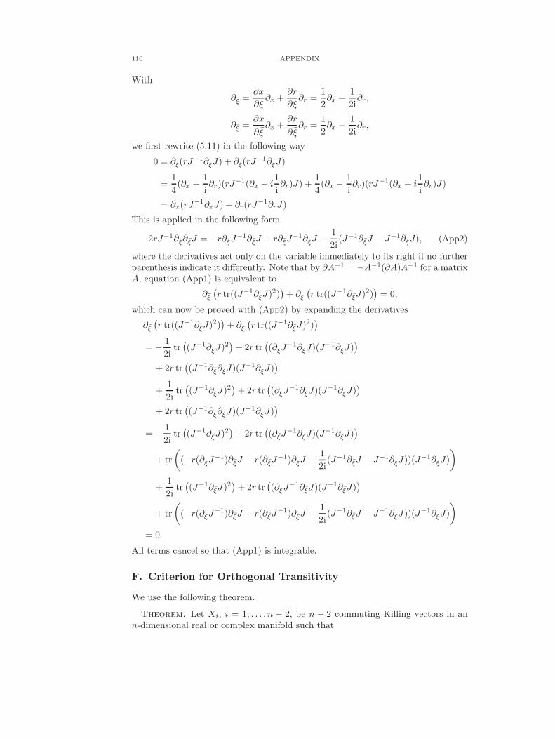
110 APPENDIX

With

∂ξ =∂x

∂ξ∂x +

∂r

∂ξ∂r =

1

2∂x +

1

2i∂r,

∂ξ =∂x

∂ξ∂x +

∂r

∂ξ∂r =

1

2∂x − 1

2i∂r,

we first rewrite (5.11) in the following way

0 = ∂ξ(rJ−1∂ξJ) + ∂ξ(rJ

−1∂ξJ)

=1

4(∂x +

1

i∂r)(rJ

−1(∂x − i1

i∂r)J) +

1

4(∂x − 1

i∂r)(rJ

−1(∂x + i1

i∂r)J)

= ∂x(rJ−1∂xJ) + ∂r(rJ−1∂rJ)

This is applied in the following form

2rJ−1∂ξ∂ξJ = −r∂ξJ−1∂ξJ − r∂ξJ−1∂ξJ − 1

2i(J−1∂ξJ − J−1∂ξJ), (App2)

where the derivatives act only on the variable immediately to its right if no furtherparenthesis indicate it differently. Note that by ∂A−1 = −A−1(∂A)A−1 for a matrixA, equation (App1) is equivalent to

∂ξ(r tr((J−1∂ξJ)2)

)+ ∂ξ

(r tr((J−1∂ξJ)2)

)= 0,

which can now be proved with (App2) by expanding the derivatives

∂ξ(r tr((J−1∂ξJ)2)

)+ ∂ξ

(r tr((J−1∂ξJ)2)

)

= − 1

2itr((J−1∂ξJ)2

)+ 2r tr

((∂ξJ

−1∂ξJ)(J−1∂ξJ))

+ 2r tr((J−1∂ξ∂ξJ)(J−1∂ξJ)

)

+1

2itr((J−1∂ξJ)2

)+ 2r tr

((∂ξJ

−1∂ξJ)(J−1∂ξJ))

+ 2r tr((J−1∂ξ∂ξJ)(J−1∂ξJ)

)

= − 1

2itr((J−1∂ξJ)2

)+ 2r tr

((∂ξJ

−1∂ξJ)(J−1∂ξJ))

+ tr

((−r(∂ξJ−1)∂ξJ − r(∂ξJ

−1)∂ξJ − 1

2i(J−1∂ξJ − J−1∂ξJ))(J−1∂ξJ)

)

+1

2itr((J−1∂ξJ)2

)+ 2r tr

((∂ξJ

−1∂ξJ)(J−1∂ξJ))

+ tr

((−r(∂ξJ−1)∂ξJ − r(∂ξJ

−1)∂ξJ − 1

2i(J−1∂ξJ − J−1∂ξJ))(J−1∂ξJ)

)

= 0

All terms cancel so that (App1) is integrable.

F. Criterion for Orthogonal Transitivity

We use the following theorem.

Theorem. Let Xi, i = 1, . . . , n − 2, be n − 2 commuting Killing vectors in ann-dimensional real or complex manifold such that

H. ROD STRUCTURE OF SCHWARZSCHILD SOLUTION 111

(1) the tensor X[a1

1 Xa2

2 · · ·Xan−2

n−2 ∇bXc]i vanishes at least at one point for every

i = 1, . . . , n− 2 and

(2) the tensor XciR

[bc X

a1

1 Xa2

2 · · ·Xan−2]n−2 = 0 for all i = 1, . . . , n− 2,

then the 2-planes orthogonal to the Killing vectors Xi, i = 1, . . . , n − 2, are inte-grable.

For dimension four this is proven in [45, Thm. 7.1.1] using Frobenius’ theoremon integrable submanifolds; the generalization is due to Emparan and Reall [11].In the Einstein vacuum case condition (2) is automatically satisfied. Condition(1) is moreover satisfied if for example one of the Killing vectors corresponds to anaxisymmetry, hence it vanishes on its “rotation axis”. If we suppose both holds, thenthe obtain the metric in the σ-model form. In the real case we want our space-timealso stationary (to get isothermal coordinates on space-time modulo symmetries).

G. Conical Singularities

Suppose we parameterize the flat, real, three-dimensional space in conical coordi-nates. Then the metric takes the form

dx2 + dy2 + dz2 = dr2 + k2r2dϕ2 + dz2,

which is singular at r = 0. Apparently, this is only a coordinate effect. So, con-versely given a metric

dr2 + k2r2dϕ2 + dz2

we can define x = r cos θ, y = r sin θ, θ = kϕ so that

dr2 + k2r2dϕ2 + dz2 = dx2 + dy2 + dz2.

However, this requires that the periodicities of ϕ and θ are in a ratio of 2πk

. If theydo not have the correct periodicity, then a singularity at the apex z = 0, r = 0appears which is of the form “Riem = δ(r)”. That is, there are diffeomorphisminvariant quantities which become singular at the origin but their limit towards itis finite. Lastly, a short picture how the above form of the metric relates to thepicture of a cone. In cylinder coordinates

dR2 +R2dϕ2 + dZ2

a cone with aperture 2α is given by Z = R cotα, see Figure 1. With dZ2 = dR2 cotαthe metric on the cone becomes

sin−2 α dR2 +R2dϕ2 = dr2 + sin2 α r2dϕ2

where R = r sinα. This is exactly our conical parameterization of the (x, y)-planeabove with the relation k2 = sin2 α.

H. Rod Structure of Schwarzschild Solution

With the substitution

z = (R−m) cos Θ, r = (R2 − 2mR)12 sin Θ, t = T, θ = Φ

for the Schwarzschild metric

ds2 =

(1 − 2m

R

)dT 2 −

(1 − 2m

R

)−1

dR2 −R2(dΘ2 + sin2 Θ dΦ2)

112 APPENDIX

α

z

y

x

Figure 1. Cone with aperture 2α.

we calculate

(z +m)2 = (R cos Θ +m(1 − cos Θ))2

= R2 cos2 Θ + 2mR cos Θ(1 − cos Θ) +m2(1 − cos Θ)2,

(z −m)2 = (R cos Θ −m(1 + cos Θ))2

= R2 cos2 Θ − 2mR cos Θ(1 + cos Θ) +m2(1 + cos Θ)2,

r2 = R2 sin2 Θ − 2mR sin2 Θ.

This yields

r2 + (z +m)2 = R2 + 2mR(cos Θ − 1) +m2(1 − cos Θ)2

= (R+m(cos Θ − 1))2 ,

r2 + (z −m)2 = R2 − 2mR(cos Θ + 1) +m2(1 + cos Θ)2

= (R−m(cos Θ + 1))2,

and therefore

r+ + r− = 2R− 2m and f =2R− 4m

2R= 1 − 2m

R.

But from the metric we see

g(Y, Y ) = 1 − 2m

R,

and

g(X,X) = −R2 sin2 Θ = − (R2 − 2mR)R2 sin2 Θ

R2 − 2mR= − (R2 − 2mR) sin2 Θ

1 − 2mR

= −r2

f.

Then J takes the desired form.

I. GENERAL BÄCKLUND TRANSFORMATION 113

I. General Bäcklund Transformation

Starting from the given decomposition we have2

J−1 =

A−1 0

B 1

−1 1 B

0 A−1

,

and

∂αJ = −

1 B

0 A−1

−1 0 Bα

0 −A−1AαA−1

1 B

0 A−1

−1 A−1 0

B 1

+

1 B

0 A−1

−1 −A−1AαA

−1 0

Bα 0

,

where α ∈ w, z. This yields

J−1∂αJ

= −

A−1 0

B 1

−1 0 Bα

0 −A−1AαA−1

1 B

0 A−1

−1 A−1 0

B 1

+

A−1 0

B 1

−1 −A−1AαA

−1 0

Bα 0

= −

A 0

−BA 1

0 Bα

0 −A−1AαA−1

1 −BA

0 A

A−1 0

B 1

+

A 0

−BA 1

−A−1AαA

−1 0

Bα 0

=

−ABαAB −AαA−1 −ABαA

BABαAB + A−1AαB +BAαA−1 +Bα BABαA+ A−1Aα

.

From this we can read off the form of Yang’s equation (5.2). The (12)-entry of thematrix yields


which is the second equation in (8.2). Using this we get for the (11)-entry

ABzABz + ∂z(AzA−1) −ABwABw − ∂w(AwA

−1) = 0,

which corresponds to the last equation in (8.2). Again using ABαA = 0 we get forthe (22)-entry

BzABzA+ ∂z(A−1Az) −BwABwA− ∂w(A−1Aw) = 0

2Using

(A−1 0B 1

)−1

=

(A 0

−BA 1

).

114 APPENDIX

corresponding to the third equation in (8.2). Lastly, with the vanishing of the(11)-entry we obtain for the (21)-entry

0 = (BABzA+ A−1Az)Bz + (BAzA−1)z + (A−1)zABz + A−1(ABzA)zA

−1

+BzA(A−1)z − (z, z ↔ w, w)

= A−1AzBz +BzAzA−1 + (A−1)zABz +BzA(A−1)z

+ A−1(ABzA)zA−1 − (z, z ↔ w, w)

= A−1(AzBz − AzBz) + (BzAz −BzAz)A−1

+ A−1(ABzA)zA−1 − (z, z ↔ w, w).

Multiplying with A from left and A from right gives

0 = (AzBz − AzBz)A+ A(BzAz −BzAz) + (ABzA)z − (z, z ↔ w, w)

= (ABzA)z − ABzzA− (ABzA)z + ABzzA+ (ABzA)z − (z, z ↔ w, w)

= (ABzA)z − (ABwA)w,

that is the first equation in (8.2).

J. Reduced Bäcklund Transformation

To obtain the reduced form of the Yang’s equation in terms of the Bäcklund de-composition we proceed as above. By taking α ∈ r, x we immediately get the lastthree equations and the part with the x-derivatives in the first equation. Only ther-derivatives in the first equation need a closer look. But there we have in the sameway as above

r(BABrA+ A−1Ar)Br + (rBArA−1)r + (rA−1ABrAA

−1)r

= rA−1ArBr + rBrArA−1 + r(A−1)rABr + rBrA(A−1)r

+ A−1(rABrA)rA−1

= rA−1(ArBr − ArBr) + r(BrAr −BrAr)A−1 + A−1(rABrA)rA

−1

= A−1(rABrA)rA−1,

which yields the claimed form of the equations.

J.1. Two-Nut Spacetime: Parameter Configurations. Given the set ofparameters (α > 0, L1, L2), we would like to see whether the mass, that is c3, isuniquely determined. If we set x = c3, then from (10.13) we get

4α2x4 =

(x3 − L2

2

)2

− L21L

22

with 2Li = πLi and L2 = L21 + L2

2. This is equivalent to finding the positive zerosof

F (x) ≔ x6 − 4α2x4 − L2x3 +1

4

(L2

1 − L22

)2.

K. IMPLICATIONS OF HYPERSURFACE-ORTHOGONALITY 115

Rewrite this as

F (x) = x3(x3 − 4α2x− L2

)︸︷︷︸

G(x)

+K, where K =1

4

(L2

1 − L22

)2 ≥ 0.

NowG′(x) = x2 (6x3 − 16α2x− 3L2)︸︷︷︸

g(x)

Since g(x) is a third order polynomial with positive leading coefficient, and negativevalue and slope for x = 0, it has to have precisely one zero for x > 0. Therefore,G(x) has precisely two extremal points for x < 0, a saddle point at the origin andprecisely one minimum for x > 0. At this minimum it is

x3 =8

3α2x+

1

2L2

∣∣∣∣xmin>0

,

hence

G(x)|xmin>0 =

(8

3α2x+

1

2L2

)(−4

3α2x− 1

2L2

)= −32

9α4x2 − 2α2L2x− 1

4L4.

Finally, we see that

F (x)|xmin>0 = G(x)|xmin>0 +K = −32

9α4x2 − 2α2L2x− L2

1L22 < 0,

and because G(0) = 0, we conclude that with no conditions on (α > 0, L1, L2) thereare two positive solutions for x (unless L2

1 = L22 when there is only one).

K. Implications of Hypersurface-Orthogonality

A Killing vector K is called hypersurface-orthogonal if K is the normal of a hyper-surface. By [45, Thm. B.3.2] this is equivalent to the vanishing K ∧ dK, where wedenote the Killing 1-form by K as well. To sketch how this implies the vanishing ofcertain metric coefficients we write in our case

Ψ = gtψ dt+ gϕψ dϕ+ gψψ dψ,

thendΨ = gtψ,r dr ∧ dt+ gϕψ,r dr ∧ dϕ+ gψψ,r dr ∧ dψ + r ↔ z

and Ψ ∧ dΨ = 0 is equivalent to

gϕψ dgtψ = gtψ dgϕψ,

gψψ dgtψ = gtψ dgψψ,

gψψ dgϕψ = gϕψ dgψψ,

where d = ∂r + ∂z. If all three of the metric coefficients are non-zero these equa-tions can be integrated easily, showing that all three metric coefficients have tobe proportional. However, this is a contradiction with respect to the asymptoticform of the metric if we regard this set of equations for a region that extends to√r2 + z2 → ∞. Thus, some of the metric coefficients have to vanish, and it is not

hard to see that the only possibility, which is compatible with the asymptotic formof the metric, is when gtψ = gϕψ = 0.

Bibliography

[1] O. Aharony, S. S. Gubser, J. M. Maldacena, H. Ooguri, & Y. Oz. Large NField Theories, String Theory and Gravity. Phys. Rept., 323:183–386, 2000,hep-th/9905111.

[2] J. M. Bardeen, B. Carter, & S. W. Hawking. The Four Laws of Black HoleMechanics. Comm. Math. Phys., 31:161–170, 1973.

[3] V. A. Belinskiı & V. E. Zakharov. Integration of the Einstein Equations byMeans of the Inverse Scattering Problem Technique and Construction of ExactSoliton Solutions. Sov. Phys. JETP, 48(6):985, 1978.

[4] B. Carter. Axisymmetric Black Hole Has Only Two Degrees of Freedom. Phys.Rev. Lett., 26:331–333, Feb 1971.

[5] Y. Chen & E. Teo. A Rotating Black Lens Solution in Five Dimensions. Phys.Rev., D78:064062, 2008, gr-qc/0808.0587.

[6] P. T. Chruściel & J. L. Costa. On Uniqueness of Stationary Vacuum BlackHoles. Astérisque, 321:195–265, 2008, gr-qc/0806.0016. Géométrie différen-tielle, physique mathématique, mathématiques et société. I.

[7] P. T. Chruściel & L. Nguyen. A Lower Bound for the Mass of AxisymmetricConnected Black Hole Data Sets. Class. Quant. Grav., 28:125001, 2011, gr-qc/1102.1175.

[8] H. Elvang & P. Figueras. Black Saturn. JHEP, 05:050, 2007, hep-th/0701035.

[9] H. Elvang, R. Emparan, & A. Virmani. Dynamics and Stability of Black Rings.J. High Energy Phys., 12:074, 35 pp. (electronic), 2006, hep-th/0608076.

[10] R. Emparan & H. S. Reall. A Rotating Black Ring Solution in Five Dimensions.Phys. Rev. Lett., 88(10):101101, 2002, hep-th/0110260.

[11] R. Emparan & H. S. Reall. Generalized Weyl Solutions. Phys. Rev. D (3), 65(8):084025, 26, 2002, hep-th/0110258.

[12] R. Emparan & H. S. Reall. Black Rings. Classical Quantum Gravity, 23(20):R169–R197, 2006, hep-th/0608012.

[13] R. Emparan & H. S. Reall. Black Holes in Higher Dimensions. Living Reviews inRelativity, 11(6), 2008. URL http://www.livingreviews.org/lrr-2008-6.

[14] F. J. Ernst. New Formulation of the Axially Symmetric Gravitational FieldProblem. Phys. Rev., 167:1175–1178, Mar 1968.

[15] M. Field. Several Complex Variables and Complex Manifolds. Number pt. 1in London Mathematical Society Lecture Note Series. Cambridge UniversityPress, 1982.

117

http://www.livingreviews.org/lrr-2008-6

118 Bibliography

[16] J. Fletcher. Non-Hausdorff Twistor Spaces and the Global Structure of Space-Time. PhD thesis, Oxford University (England), 1990.

[17] J. Fletcher & N. M. J. Woodhouse. Twistor Characterization of StationaryAxisymmetric Solutions of Einstein’s Equations. In Twistors in Mathematicsand Physics, Volume 156 of London Math. Soc. Lecture Note Ser., pages 260–282. Cambridge University Press, Cambridge, 1990.

[18] K. Fritzsche & H. Grauert. From Holomorphic Functions to Complex Mani-folds. Graduate Texts in Mathematics. Springer, 2002.

[19] S. Giusto & A. Saxena. Stationary Axisymmetric Solutions of Five DimensionalGravity. Class.Quant.Grav., 24:4269–4294, 2007, hep-th/0705.4484.

[20] H. Grauert, T. Peternell, & R. Remmert. Several Complex Variables VII: Sheaf-Theoretical Methods in Complex Analysis. Number v. 74 in Encyclopaedia ofMathematical Sciences. Springer-Verlag, 1994.

[21] T. Harmark. Stationary and Axisymmetric Solutions of Higher-DimensionalGeneral Relativity. Phys. Rev. D (3), 70(12):124002, 25, 2004, hep-th/0408141.

[22] S. W. Hawking. Black Holes in General Relativity. Comm. Math. Phys., 25:152–166, 1972.

[23] S. W. Hawking & G. F. R. Ellis. The Large Scale Structure of Space-Time.Cambridge University Press, London, 1973.

[24] S. Hollands & S. Yazadjiev. Uniqueness Theorem for 5-Dimensional BlackHoles with Two Axial Killing Fields. Comm. Math. Phys., 283(3):749–768,2008, gr-qc/0707.2775.

[25] S. Hollands, A. Ishibashi, & R. Wald. A Higher-Dimensional Stationary Ro-tating Black Hole Must be Axisymmetric. Communications in MathematicalPhysics, 271:699–722, 2007, gr-qc/0605106.

[26] W. Israel. Event Horizons in Static Electrovac Space-Times. Communicationsin Mathematical Physics, 8:245–260, 1968.

[27] P. Kanti. Black Holes in Theories with Large Extra Dimensions: A Review.Int.J.Mod.Phys., A19:4899–4951, 2004, hep-ph/0402168.

[28] C. Klein & O. Richter. Ernst Equation and Riemann Surfaces, Volume 685 ofLecture Notes in Physics. Springer-Verlag, Berlin, 2005.

[29] S. Kobayashi & K. Nomizu. Foundations of Differential Geometry, Volume Iof Wiley Classics Library. John Wiley & Sons Inc., New York, 1996.

[30] S. Kobayashi & K. Nomizu. Foundations of Differential Geometry, Volume IIof Wiley Classics Library. John Wiley & Sons Inc., New York, 1996.

[31] D. Maison. Ehlers-Harrison-Type Transformations for Jordan’s Extended The-ory of Gravitation. Gen. Relativity Gravitation, 10(8):717–723, 1979.

[32] J. M. Maldacena. The Large N Limit of Superconformal Field Theories andSupergravity. Adv.Theor.Math.Phys., 2:231–252, 1998, hep-th/9711200.

[33] L. J. Mason & N. M. J. Woodhouse. Integrability, Self-Duality, and TwistorTheory. London Mathematical Society Monographs. New Series. The Claren-don Press Oxford University Press, New York, 1996.

Bibliography 119

[34] R. Myers & M. Perry. Black Holes in Higher-Dimensional Space-Times. Annalsof Physics, 172(2):304 – 347, 1986.

[35] R. C. Myers. Myers-Perry Black Holes, 2011, gr-qc/1111.1903.

[36] R. Penrose. The Road to Reality: A Complete Guide to the Laws of the Uni-verse. Vintage, 2007.

[37] A. Pomeransky & R. Sen’kov. Black Ring with Two Angular Momenta, 2006,hep-th/0612005.

[38] A. D. Popov. Self-Dual Yang-Mills: Symmetries and Moduli Space. Rev. Math.Phys., 11:1091, 1999, hep-th/9803183.

[39] D. C. Robinson. Uniqueness of the Kerr Black Hole. Phys. Rev. Lett., 34:905–906, Apr 1975.

[40] A. Strominger & C. Vafa. Microscopic Origin of the Bekenstein-Hawking En-tropy. Phys. Lett., B379:99–104, 1996, hep-th/9601029.

[41] D. Sudarsky & R. M. Wald. Extrema of Mass, Stationarity, and Staticity, andSolutions to the Einstein-Yang-Mills Equations. Phys. Rev. D, 46:1453–1474,Aug 1992.

[42] S. Tomizawa, Y. Uchida, & T. Shiromizu. Twist of a Stationary Black Holeor Ring in Dive Dimensions. Phys. Rev. D (3), 70(6):064020, 5, 2004, gr-qc/0405134.

[43] S. Tomizawa, Y. Yasui, & A. Ishibashi. Uniqueness Theorem for ChargedRotating Black Holes in Five-Dimensional Minimal Supergravity. Phys. Rev.D, 79:124023, Jun 2009, hep-th/0901.4724.

[44] P. K. Townsend. Black Holes (Lecture Notes Part III), 1997. URLhttp://arxiv.org/pdf/gr-qc/9707012v1.

[45] R. M. Wald. General Relativity. University of Chicago Press, Chicago, IL,1984.

[46] R. S. Ward. Stationary Axisymmetric Space-Times: A New Approach. Gen.Relativity Gravitation, 15(2):105–109, 1983.

[47] R. Ward. On Self-Dual Gauge Fields. Physics Letters A, 61(2):81 – 82, 1977.

[48] L. Witten. Static Axially Symmetric Solutions of Self-Dual SU(2) Gauge Fieldsin Euclidean Four-Dimensional Space. Phys. Rev. D, 19:718–720, Jan 1979.

[49] N. M. J. Woodhouse & L. J. Mason. The Geroch Group and Non-HausdorffTwistor Spaces. Nonlinearity, 1(1):73–114, 1988.

[50] C. N. Yang. Condition of Self-Duality for SU(2) Gauge Fields on EuclideanFour-Dimensional Space. Phys. Rev. Lett., 38:1377–1379, Jun 1977.

http://arxiv.org/pdf/gr-qc/9707012v1

twistor theory of higher-dimensional black holes

Documents