hades rv programme with harps-n at tng - arxiv · astronomy & astrophysics manuscript no....
TRANSCRIPT

Astronomy & Astrophysics manuscript no. GJ625_AA_vArxiv c©ESO 2017June 14, 2017
HADES RV Programme with HARPS-N at TNG
V. A super-Earth on the inner edge of the habitable zone of the nearby M-dwarfGJ 625 ?
A. Suárez Mascareño1, 2, 3, J. I. González Hernández1, 3, R. Rebolo1, 3, 4, S. Velasco1, 3, B. Toledo-Padrón1, 3, L. Affer5,M. Perger6, G. Micela5, I. Ribas6, J. Maldonado5, G. Leto7, R. Zanmar Sanchez7, G. Scandariato7, M. Damasso8, A.
Sozzetti8, M. Esposito9, E. Covino9, A. Maggio5, A. F. Lanza7, S. Desidera10, A. Rosich6, A. Bignamini11, R.Claudi10, S. Benatti10, F. Borsa12, M. Pedani13, E. Molinari13, J. C. Morales6, E. Herrero6, and M. Lafarga6
1 Instituto de Astrofísica de Canarias, E-38205 La Laguna, Tenerife, Spaine-mail: [email protected]
2 Observatoire Astronomique de l’Université de Genève, Versoix, Switzerlande-mail: [email protected]
3 Universidad de La Laguna, Dpto. Astrofísica, E-38206 La Laguna, Tenerife, Spain4 Consejo Superior de Investigaciones Científicas, Spain5 INAF - Osservatorio Astronomico di Palermo, Piazza del Parlamento 1, 90134 Palermo, Italy6 Institut de Ciènces de l’Espai (CSIC-IEEC), Campus UAB, Carrer de Can Magrans s/n, 08193 Cerdanyola del Vallés, Spain7 INAF - Osservatorio Astrofisico di Catania, via S. Sofia 78, 95123 Catania, Italy8 INAF - Osservatorio Astrofisico di Torino, via Osservatorio 20, 10025 Pino Torinese, Italy9 INAF - Osservatorio Astronomico di Capodimonte, Via Moiariello, 16, 80131 - NAPOLI
10 INAF - Osservatorio Astronomico di Padova, Vicolo dell’Osservatorio 5, 35122, Padova, Italy11 INAF - Osservatorio Astronomico di Trieste, via Tiepolo 11,34143, Trieste, Italy12 INAF - Osservatorio Astronomico di Brera, Via E. Bianchi 46,I-23807 Merate (LC), Italy13 Fundación Galileo Galilei - INAF, Rambla José Ana Fernandez Pérez 7, E-38712 Breña Baja, TF - Spain
Revised April-2017
ABSTRACT
We report the discovery of a super-Earth orbiting at the inner edge of the habitable zone of the star GJ 625 based on the analysis of theradial-velocity (RV) time series from the HARPS-N spectrograph, consisting in 151 HARPS-N measurements taken over 3.5 yr. GJ625 b is a planet with a minimum mass M sin i of 2.82 ± 0.51 M⊕ with an orbital period of 14.628 ± 0.013 days at a distance of 0.078AU of its parent star. The host star is the quiet M2 V star GJ 625, located at 6.5 pc from the Sun. We find the presence of a secondradial velocity signal in the range 74-85 days that we relate to stellar rotation after analysing the time series of Ca II H&K and Hαspectroscopic indicators, the variations of the FWHM of the CCF and and the APT2 photometric light curves. We find no evidencelinking the short period radial velocity signal to any activity proxy.
Key words. Planetary Systems — Techniques: radial velocity — Stars: activity — Stars: chromospheres — Stars: rotation — Stars:magnetic cycle — starspots — Stars: individual (GJ 625)
1. Introduction
The detection rate of potentially habitable Earth-like planetsaround M-dwarfs is rapidly increasing (Wright et al. 2016;Anglada-Escudé et al. 2016; Jehin et al. 2016; Gillon et al. 2017;Astudillo-Defru et al. 2017). Since years ago it has been clearthat M-dwarfs are a shortcut to find earth-like planets and there-fore several surveys have attempted to take advantage of their
? Based on: observations made with the Italian Telescopio NazionaleGalileo (TNG), operated on the island of La Palma by the INAF - Fun-dación Galileo Galilei at the Roche de Los Muchachos Observatory ofthe Instituto de Astrofísica de Canarias (IAC); photometric observationsmade with the robotic telescope APT2 (within the EXORAP program)located at Serra La Nave on Mt. Etna.; lucky imaging observations madewith the Telescopio Carlos Sánchez operated on the island of Tenerifeby the Instituto de Astrofísica de Canarias in the Spanish Observatoriodel Teide.
low masses and closer habitable zones (Quirrenbach et al. 2012;Bonfils et al. 2013; Howard et al. 2014; Irwin et al. 2015; Berta-Thompson et al. 2015a; Affer et al. 2016; Suárez Mascareñoet al. 2017a; Perger et al. 2017b). M-dwarfs have also provento be difficult targets because of their stellar activity. The sig-nals induced by the stellar rotation can easily mimic those ofplanetary origin (Queloz et al. 2001; Bonfils et al. 2007; Boisseet al. 2011; Robertson et al. 2014; Suárez Mascareño et al. 2015;Newton et al. 2016; Vanderburg et al. 2016; Suárez Mascareñoet al. 2017a,b). For the case of M-dwarfs these signals tend to becomparable to those of rocky planets close to the habitable zoneof their stars (Howard et al. 2014; Robertson et al. 2014; SuárezMascareño et al. 2015; Newton et al. 2016; Suárez Mascareñoet al. 2017b). The interpretation of the radial velocity curves ofM-dwarfs is usually complicated even in the quietest of stars.Low mass stars are the most common type of stars, offering valu-able complementary information on the formation mechanisms
Article number, page 1 of 22
arX
iv:1
705.
0653
7v3
[as
tro-
ph.E
P] 1
3 Ju
n 20
17
A&A proofs: manuscript no. GJ625_AA_vArxiv
of planetary systems. For instance giant planets at close orbitsare known to be rare around M dwarfs (Endl et al. 2006), whilelow mass rocky planets appear to be more frequent (Bonfils et al.2013; Dressing & Charbonneau 2013; Dressing et al. 2015).
Even with the large amount of confirmed exoplanets(Howard et al. 2009; Mayor et al. 2011; Howard et al. 2012) thenumber of rocky planets remains comparably small with onlyabout a hundred known around M-dwarfs. This is mostly be-cause most surveys – including the Kepler survey – have fo-cused primarily in solar type and K-type stars. In the recentyears many planetary systems have been reported hosting Nep-tune mass planets and super-Earths (Udry et al. 2007; Delfosseet al. 2013; Howard et al. 2014; Astudillo-Defru et al. 2015), anda rapidly increasing amount of Earth-mass planets (Mayor et al.2009; Berta-Thompson et al. 2015b; Wright et al. 2016; Afferet al. 2016; Anglada-Escudé et al. 2016; Jehin et al. 2016; SuárezMascareño et al. 2017a; Gillon et al. 2017). However the fre-quency of Earth-sized planets around M-dwarfs is still not wellestablished. Several studies have attempted to quantify the abun-dance of rocky planets in close orbits and in the habitable zonesof M-dwarfs, but the uncertainties are still large, making it im-portant to continue adding new planets to the sample (Bonfilset al. 2013; Gaidos 2013; Kopparapu 2013).
We report the discovery of a super-Earth orbiting the nearbystar GJ 625 on the inner edge of its habitable zone. The discov-ery is part of the HADES (HArps-n red Dwarf Exoplanet Sur-vey) radial velocity (RV) program with HARPS-N at the Tele-scopio Nazionale Galileo in La Palma (Spain). The HADES RVprogram is the result of a collaborative effort between the Ital-ian Global Architecture of Planetary Systems (GAPS, Covinoet al. (2013); Poretti et al. (2016)) Consortium, The Institut deCiències de l’Espai de Catalunya (ICE), and the Instituto de As-trofísica de Canarias (IAC). The HADES team has previouslydiscovered two super-Earth exoplanets of minimum masses of∼ 6.3 and ∼ 2.5 M⊕ orbiting the early-type M-dwarf GJ 3998(Affer et al. 2016).
GJ 625 is a bright (V = 10.17 mag) low activity (log10(R′HK)∼ – 5.5) M-dwarf located at a distance of 6.5 pc from the Sun(van Leeuwen 2007; Gaia Collaboration et al. 2016). Table 1shows the stellar parameters. Its low activity combined with itslong rotation period, of more than 70 days, makes it a very inter-esting candidate to search for rocky planets.
2. Data & Observations
2.1. Spectroscopy
The star GJ 625 is part of the HADES RV program (Afferet al. 2016) and has been extensively monitored since 2013. Wehave used 151 HARPS-N spectra taken over 3.5 yr. HARPS-N (Cosentino et al. 2012) is a fibre-fed high resolution echellespectrograph installed at the Telescopio Nazionale Galileo inthe Roque de los Muchachos Observatory (Spain). The instru-ment has a resolving power greater than R ∼ 115 000 over aspectral range from ∼380 to ∼690 nm and has been designedto attain very high long-term radial-velocity precision. It is con-tained in a vacuum vessel to avoid spectral drifts due to tem-perature and air pressure variations, thus ensuring its stability.HARPS-N is equipped with its own pipeline providing extractedand wavelength-calibrated spectra, as well as RV measurementsand other data products such as cross-correlation functions andtheir bisector profiles.
Most of the observations were carried out using the FabryPerot (FP) as simultaneous calibration. The FP offers the pos-
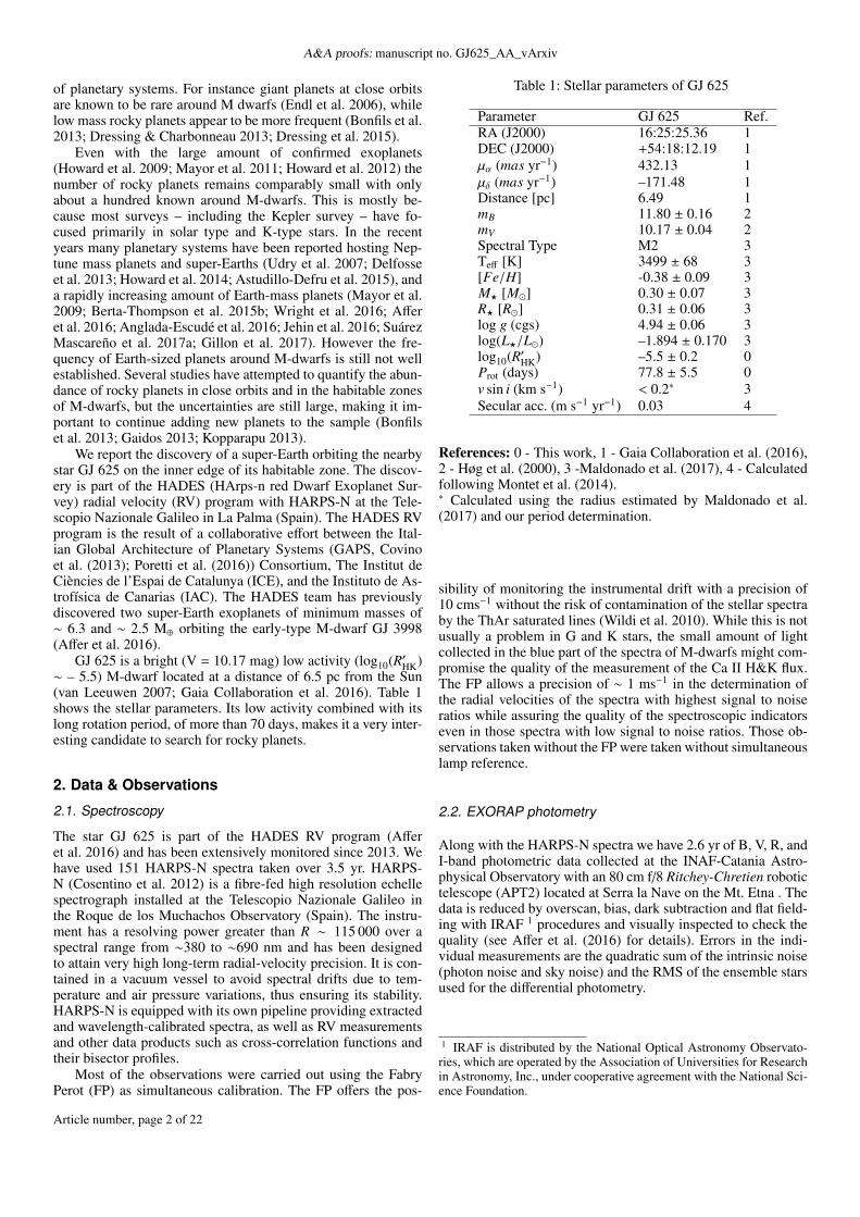
Table 1: Stellar parameters of GJ 625
Parameter GJ 625 Ref.RA (J2000) 16:25:25.36 1DEC (J2000) +54:18:12.19 1µα (mas yr−1) 432.13 1µδ (mas yr−1) –171.48 1Distance [pc] 6.49 1mB 11.80 ± 0.16 2mV 10.17 ± 0.04 2Spectral Type M2 3Teff [K] 3499 ± 68 3[Fe/H] -0.38 ± 0.09 3M? [M�] 0.30 ± 0.07 3R? [R�] 0.31 ± 0.06 3log g (cgs) 4.94 ± 0.06 3log(L?/L�) –1.894 ± 0.170 3log10(R′HK) –5.5 ± 0.2 0Prot (days) 77.8 ± 5.5 0v sin i (km s−1) < 0.2∗ 3Secular acc. (m s−1 yr−1) 0.03 4
References: 0 - This work, 1 - Gaia Collaboration et al. (2016),2 - Høg et al. (2000), 3 -Maldonado et al. (2017), 4 - Calculatedfollowing Montet et al. (2014).∗ Calculated using the radius estimated by Maldonado et al.(2017) and our period determination.
sibility of monitoring the instrumental drift with a precision of10 cms−1 without the risk of contamination of the stellar spectraby the ThAr saturated lines (Wildi et al. 2010). While this is notusually a problem in G and K stars, the small amount of lightcollected in the blue part of the spectra of M-dwarfs might com-promise the quality of the measurement of the Ca II H&K flux.The FP allows a precision of ∼ 1 ms−1 in the determination ofthe radial velocities of the spectra with highest signal to noiseratios while assuring the quality of the spectroscopic indicatorseven in those spectra with low signal to noise ratios. Those ob-servations taken without the FP were taken without simultaneouslamp reference.
2.2. EXORAP photometry
Along with the HARPS-N spectra we have 2.6 yr of B, V, R, andI-band photometric data collected at the INAF-Catania Astro-physical Observatory with an 80 cm f/8 Ritchey-Chretien robotictelescope (APT2) located at Serra la Nave on the Mt. Etna . Thedata is reduced by overscan, bias, dark subtraction and flat field-ing with IRAF 1 procedures and visually inspected to check thequality (see Affer et al. (2016) for details). Errors in the indi-vidual measurements are the quadratic sum of the intrinsic noise(photon noise and sky noise) and the RMS of the ensemble starsused for the differential photometry.
1 IRAF is distributed by the National Optical Astronomy Observato-ries, which are operated by the Association of Universities for Researchin Astronomy, Inc., under cooperative agreement with the National Sci-ence Foundation.
Article number, page 2 of 22

A. Suárez Mascareño et al.: HADES RV Programme with HARPS-N at TNG
Fig. 1: Diffraction-limited image of GJ 625 after lucky imag-ing processing with a selection of the 30% best individualTCS/FastCam frames.
2.3. FastCam Lucky Imaging Observations
On June 6th 2016, we collected 50,000 individual frames of GJ625 in the I band using the lucky imaging FastCam instrument(Oscoz et al. 2008) at the 1.5m Carlos Sánchez Telescope in theObservatorio del Teide, Tenerife, with 30 ms exposure time foreach frame. FastCam is an optical imager with a low noise EM-CCD camera which allows to obtain speckle-featuring not satu-rated images at a fast frame rate (Labadie et al. 2011).
In order to construct a high resolution, diffraction lim-ited, long-exposure image, the individual frames were bias sub-tracted, aligned and co-added using our own Lucky Imaging al-gorithm (Velasco et al. 2016). Figure 1 presents the high reso-lution image constructed by co-addition of the best percentageof the images using lucky imaging and shift-and-add algorithms.Due to the atmospheric conditions of the night, the selection of30% of the individual frames was found to be the best solutionto produce a deep and diffraction limited image of the target, re-sulting in a total integration time of 450 seconds. The combinedimage achieved ∆mI = 4.5− 5.0 at 1′′. We find no bright contam-inant star in the diffraction limited image.
3. Determination of Stellar Activity Indicators andRadial Velocities
3.1. Activity Indicators
For the activity analysis we use the extracted order-by-order wavelength-calibrated spectra produced by the HARPS-N pipeline. For a given star, the change in atmospheric trans-parency from day to day causes variations in the flux distribu-tion of the recorded spectra that are particularly relevant in theblue, where we intend to measure Ca II lines. In order to mini-mize the effects related to these atmospheric changes we createa spectral template for each star by de-blazing and co-adding ev-ery available spectrum and use the co-added spectrum to correctthe order-by-order fluxes of the individual ones. We also correcteach spectrum for the Earth’s barycentric radial velocity and theradial velocity of the star using the measurements given by the
CaII K line
3932 3933 3934 3935Wavelength (Å)
0.0
0.5
1.0
1.5
2.0
2.5
Rel
ativ
e F
lux
CaII H line
3967 3968 3969 3970Wavelength (Å)
0.0
0.5
1.0
1.5
2.0
2.5
Rel
ativ
e F
lux
Continuum V
3885 3890 3895 3900 3905 3910 3915Wavelength (Å)
0.0
0.5
1.0
1.5
2.0
2.5
Rel
ativ
e F
lux
Continuum R
3985 3990 3995 4000 4005 4010 4015Wavelength (Å)
0.0
0.5
1.0
1.5
2.0
2.5
Rel
ativ
e F
lux
Fig. 2: Ca II H&K filter of the spectrum of the star GJ 625 withthe same shape as the Mount Wilson Ca II H&K passband.
standard pipeline and re-binned the spectra into a wavelength-constant step. Using this HARPS-N dataset, we expect to havehigh quality spectroscopic indicators to monitor tiny stellar ac-tivity variations with high accuracy.
SMW Index
We calculate the Mount Wilson S index and the log10(R′HK) byusing the original Noyes et al. (1984) procedure, following Lo-vis et al. (2011) and Suárez Mascareño et al. (2015, 2017a). Wedefine two triangular-shaped passbands with full width half max-imum (FWHM) of 1.09 Å centred at 3968.470 Å and 3933.664 Åfor the Ca II H&K line cores, and for the continuum we use two20 Å wide bands centred at 3901.070 Å (V) and 4001.070 Å(R),as shown in figure 2.
Then the S-index is defined as
S = αNH + NK
NR + NV+ β, (1)
where NH , NK , NR and NV are the mean fluxes per wavelengthunit in each passband, while α and β are calibration constantsfixed as α = 1.111 and β = 0.0153 . The S index (SMW ) servesas a measurement of the Ca II H&K core flux normalized to theneighbour continuum. As a normalized index to compare it toother stars we compute the log10(R′HK) following Suárez Mas-careño et al. (2015).
Hα Index
We also use the Hα index, with a simpler passband follow-ing Gomes da Silva et al. (2011) and Suárez Mascareño et al.(2017a). It consists of a rectangular bandpass with a width of1.6 Å and centred at 6562.808 Å (core), and two continuumbands of 10.75 Å and a 8.75 Å wide centred at 6550.87 Å (L)and 6580.31 Å (R), respectively, as seen in Figure 3.
Thus, the Hα index is defined as
HαIndex =Hαcore
HαL + HαR. (2)
Article number, page 3 of 22

A&A proofs: manuscript no. GJ625_AA_vArxiv
Fig. 3: Spectrum of the M-type star GJ 625 showing the Hα re-gion of the spectrum. The light-red shaded regions show the filterpassband and continuum bands.
Where Hαcore, HαL and HαR are the mean fluxes per wave-length unit in each of the previously defined passbands.
3.2. Radial velocities
The radial-velocity measurement in the HARPS-N standardpipeline is determined by a Gaussian fit of the cross correlationfunction (CCF) of the spectrum with a synthetic stellar template(Baranne et al. 1996; Pepe et al. 2000) that consists on a se-ries of delta functions at the positions of isolated stellar lines atwavelength longer than 4400 Å. In the case of M-dwarfs, dueto the huge number of line blends, the cross correlation functionis not Gaussian, resulting in a less precise Gaussian fit whichmight cause distortions in the radial-velocity measurements anddecrease the sensibility in the measurement of the variations inthe full width half maximum (FWHM) of the CCF. To deal withthis issue we tried two different approaches as in Suárez Mas-careño et al. (2017a).
The first one consisted in using a slightly more complexmodel for the CCF fitting, a Gaussian function plus a secondorder polynomial using only the central region of the CCF func-tion. We use a 15 km s−1 window centred at the minimum of theCCF. This configuration provides the best stability of the mea-surements. Along with the measurements of the radial velocity,we obtain the FWHM of the cross correlation function whichwe also use to track variations in the activity level of the star.A second approach to the problem was to recompute the radialvelocities using the TERRA pipeline (Anglada-Escudé & Butler2012), which is a template matching algorithm with a high sig-nal to noise stellar spectral template. Every spectrum is correctedfor both barycentric and stellar radial velocity to align it to theframe of the solar system barycenter. The radial velocities arecomputed by minimizing the χ2 of the residuals between the ob-served spectra and shifted versions of the stellar template, withall the elements contaminated by telluric lines masked. In thiscase we are using the Doppler information at wavelength longerthan 4550 Å. All radial-velocity measurements are correctedfrom the secular acceleration of the star.
For the bisector span measurement we rely on the pipelineresults, as it does not depend on the fit but on the CCF itself. Thebisector has been a standard activity diagnostic tool for solar typestars since more than 10 years ago . Unfortunately its behaviourin slow rotating stars is not as informative as it is for fast rota-tors (Saar & Donahue 1997; Bonfils et al. 2007). We report themeasurements of the bisector span (BIS) for each radial-velocity
measurement, but we do not find any meaningful information inits analysis.
3.3. Quality Control of the Data
As the sampling rate of our data is not well suited for modellingfast events, such as flares, and their effect in the radial velocity isnot well understood, we identify and reject points likely affectedby flares by searching for an abnormal behaviour of the activityindicators (Reiners 2009). The process rejected 11 spectra thatcorrespond to flare events of the star with obvious activity en-hancement and line distortion. That leaves us with 140 HARPS-N spectroscopic observations taken over 3.3 years with a typicalexposure of 900 s and an average signal to noise ratio of 56 at5500 Å. All measurements and their uncertainties are reportedin Table A.1.
4. Analysis
In order to properly understand the behaviour of the star, ourfirst step is to analyse the different modulations present in thephotometric and spectroscopic time-series.
We search for periodic variability compatible with both stel-lar rotation and long-term magnetic cycles. We compute thepower spectrum using a Generalised Lomb Scargle Periodogram(Zechmeister & Kürster 2009) and if there is any significant pe-riodicity we fit the detected period using sinusoidal model, or adouble harmonic sinusoidal model to account for the asymmetryof some signals (Berdyugina & Järvinen 2005), with the MPFITroutine (Markwardt 2009). The model used for the preliminaryanalysis is chosen based on the reduced χ2 of the fit.
The significance of the periodogram peak is evaluated usingboth the Cumming (2004) modification of the Horne & Baliu-nas (1986) formula to obtain the spectral density thresholds fora desired false alarm probability (FAP) level and bootstrap ran-domization (Endl et al. 2001) of the data. We finally opted forthe power spectral density (PSD) levels given by the bootstrapprocess as those where the most conservative.
Radial velocities
For the analysis of the radial velocities we use both the measure-ments given by the CCF and by the TERRA pipeline. We have140 measurements distributed along 3.3 years. The star shows amean RV of -12.850 Kms−1. The CCF RV measurements showan RMS of 2.56 ms−1 with a typical uncertainty of 1.32 m s−1
while the TERRA RV measurements show an RMS of 2.57 ms−1 with a typical uncertainty of 1.24 m s−1. Figure 4 shows bothtime-series of RVs. Both sets show a very similar scatter with theTERRA data having slightly smaller error bars.
We find a clear dominant signal in the data, present in bothseries with a FAP <0.1% (although more significant in theTERRA data). The signal has a period of 14.629 ± 0.069 days inthe CCF series and 14.629 ± 0.077 days in the TERRA series, asemi amplitude of 1.85 ± 0.13 ms−1 in the CCF data, and a semiamplitude of 1.65 ± 0.18 ms−1 in the TERRA data. Figure 5shows the periodograms of both data series combined and Fig-ure 6 shows the phase folded fits of both series. When analysingthe residuals we see a structure of different signals between ∼ 65to ∼ 100 days (see Fig. 5). Of those the most significant one isnot the same in the CCF and TERRA data. The CCF data showsa 74.7 ± 1.9 d signal with a semi amplitude of 1.64 ± 0.18 ms−1
while the TERRA data shows a 85.9 ± 2.8 d signal with a semi
Article number, page 4 of 22
A. Suárez Mascareño et al.: HADES RV Programme with HARPS-N at TNG
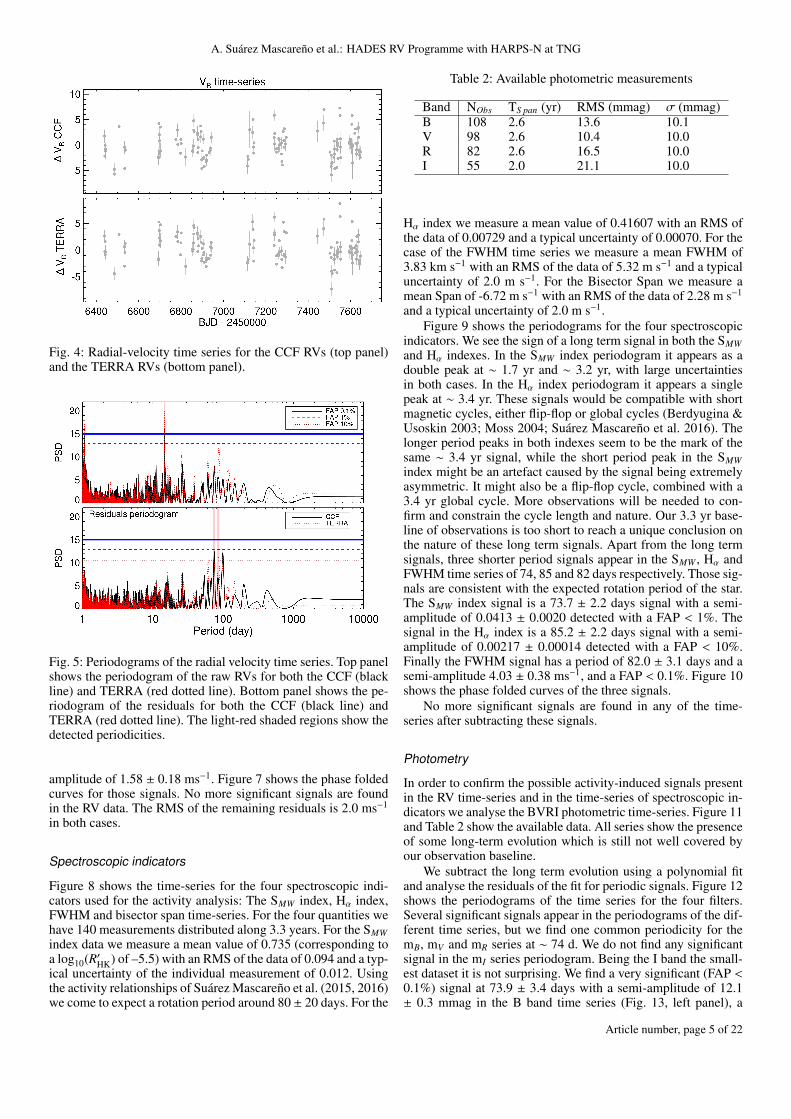
Fig. 4: Radial-velocity time series for the CCF RVs (top panel)and the TERRA RVs (bottom panel).
Fig. 5: Periodograms of the radial velocity time series. Top panelshows the periodogram of the raw RVs for both the CCF (blackline) and TERRA (red dotted line). Bottom panel shows the pe-riodogram of the residuals for both the CCF (black line) andTERRA (red dotted line). The light-red shaded regions show thedetected periodicities.
amplitude of 1.58 ± 0.18 ms−1. Figure 7 shows the phase foldedcurves for those signals. No more significant signals are foundin the RV data. The RMS of the remaining residuals is 2.0 ms−1
in both cases.
Spectroscopic indicators
Figure 8 shows the time-series for the four spectroscopic indi-cators used for the activity analysis: The SMW index, Hα index,FWHM and bisector span time-series. For the four quantities wehave 140 measurements distributed along 3.3 years. For the SMWindex data we measure a mean value of 0.735 (corresponding toa log10(R′HK) of –5.5) with an RMS of the data of 0.094 and a typ-ical uncertainty of the individual measurement of 0.012. Usingthe activity relationships of Suárez Mascareño et al. (2015, 2016)we come to expect a rotation period around 80 ± 20 days. For the
Table 2: Available photometric measurements
Band NObs TS pan (yr) RMS (mmag) σ (mmag)B 108 2.6 13.6 10.1V 98 2.6 10.4 10.0R 82 2.6 16.5 10.0I 55 2.0 21.1 10.0
Hα index we measure a mean value of 0.41607 with an RMS ofthe data of 0.00729 and a typical uncertainty of 0.00070. For thecase of the FWHM time series we measure a mean FWHM of3.83 km s−1 with an RMS of the data of 5.32 m s−1 and a typicaluncertainty of 2.0 m s−1. For the Bisector Span we measure amean Span of -6.72 m s−1 with an RMS of the data of 2.28 m s−1
and a typical uncertainty of 2.0 m s−1.Figure 9 shows the periodograms for the four spectroscopic
indicators. We see the sign of a long term signal in both the SMWand Hα indexes. In the SMW index periodogram it appears as adouble peak at ∼ 1.7 yr and ∼ 3.2 yr, with large uncertaintiesin both cases. In the Hα index periodogram it appears a singlepeak at ∼ 3.4 yr. These signals would be compatible with shortmagnetic cycles, either flip-flop or global cycles (Berdyugina &Usoskin 2003; Moss 2004; Suárez Mascareño et al. 2016). Thelonger period peaks in both indexes seem to be the mark of thesame ∼ 3.4 yr signal, while the short period peak in the SMWindex might be an artefact caused by the signal being extremelyasymmetric. It might also be a flip-flop cycle, combined with a3.4 yr global cycle. More observations will be needed to con-firm and constrain the cycle length and nature. Our 3.3 yr base-line of observations is too short to reach a unique conclusion onthe nature of these long term signals. Apart from the long termsignals, three shorter period signals appear in the SMW , Hα andFWHM time series of 74, 85 and 82 days respectively. Those sig-nals are consistent with the expected rotation period of the star.The SMW index signal is a 73.7 ± 2.2 days signal with a semi-amplitude of 0.0413 ± 0.0020 detected with a FAP < 1%. Thesignal in the Hα index is a 85.2 ± 2.2 days signal with a semi-amplitude of 0.00217 ± 0.00014 detected with a FAP < 10%.Finally the FWHM signal has a period of 82.0 ± 3.1 days and asemi-amplitude 4.03 ± 0.38 ms−1, and a FAP < 0.1%. Figure 10shows the phase folded curves of the three signals.
No more significant signals are found in any of the time-series after subtracting these signals.
Photometry
In order to confirm the possible activity-induced signals presentin the RV time-series and in the time-series of spectroscopic in-dicators we analyse the BVRI photometric time-series. Figure 11and Table 2 show the available data. All series show the presenceof some long-term evolution which is still not well covered byour observation baseline.
We subtract the long term evolution using a polynomial fitand analyse the residuals of the fit for periodic signals. Figure 12shows the periodograms of the time series for the four filters.Several significant signals appear in the periodograms of the dif-ferent time series, but we find one common periodicity for themB, mV and mR series at ∼ 74 d. We do not find any significantsignal in the mI series periodogram. Being the I band the small-est dataset it is not surprising. We find a very significant (FAP <0.1%) signal at 73.9 ± 3.4 days with a semi-amplitude of 12.1± 0.3 mmag in the B band time series (Fig. 13, left panel), a
Article number, page 5 of 22

A&A proofs: manuscript no. GJ625_AA_vArxiv
0.0 0.5 1.0 1.5 2.0-10
-5
0
5
10
VR m
s-1 C
CF
0.0 0.5 1.0 1.5 2.0Phase
-10-505
10
O -
C
0.0 0.5 1.0 1.5 2.0
-5
0
5
10
VR m
s-1 T
ER
RA
0.0 0.5 1.0 1.5 2.0Phase
-5
0
5
10
O -
C
Fig. 6: Phase folded curve of the raw RV data using the 14.6 days periodicity. Left panel shows the CCF measurements, right panelthe TERRA measurements. Red dots are the same points binned in phase with a bin size of 0.1. The error bar of a given bin isestimated using the weighted standard deviation of binned measurements divided by the square root of the number of measurementsincluded in this bin. The blue solid line shows the best fit to the data using a sinusoidal fit.
0.0 0.5 1.0 1.5 2.0
-5
0
5
VR m
s-1 C
CF
0.0 0.5 1.0 1.5 2.0Phase
-5
0
5
O -
C
0.0 0.5 1.0 1.5 2.0
-5
0
5
VR m
s-1 T
ER
RA
0.0 0.5 1.0 1.5 2.0Phase
-5
0
5
O -
C
Fig. 7: Phase folded curve of the RV data using the 74 days periodicity for the CCF data (left panel) and the 86 days periodicity forthe TERRA data (right panel) after subtracting the signals shown in Fig. 6. Red dots are the same points binned in phase with a binsize of 0.1. The error bar of a given bin is estimated using the weighted standard deviation of binned measurements divided by thesquare root of the number of measurements included in this bin. The blue solid line shows the best fit to the data using a doubleharmonic sinusoidal fit.
significant (FAP < 1%) signal at 73.9 ± 3.7 days with a semi-amplitude of 8.2 ± 0.3 mmag in the V band time series (Fig. 13,middle panel) and a less significant (FAP < 10%) signal at 73.6± 2.8 days with a semi-amplitude of 7.8 ± 0.3 mmag for the Rband time series (Fig. 13, right panel). No more significant sig-nals are found in the V and R band series after subtracting thedetected signals. For the case of the B band there is a remainingsignal at ∼ 1 yr with a second peak at ∼ 0.5 yr which seem to bean artefact.
5. Interpretation of the detected signals
The previous analysis unveiled several signals at different time-scales. Some of them are common among different datasets. Ta-
ble 3 shows the measured signals for the different datasets of GJ625. We can identify 6 different signals: At ∼3 yr, at ∼1.6 yr, at∼85 d, at ∼82 d, at ∼74 d and at ∼14.6 d.
The 3.4 yr signal appears as a significant peak in the Hα in-dex time-series and as a less significant one in the SMW indextime-series indicating a probable common origin. This signal isprobably the fingerprint of the magnetic cycle of the star. A 3.4yr cycle is short for what one could expect in solar type stars, butis in the range of previous measurements in M-dwarfs (Robert-son et al. 2013; Suárez Mascareño et al. 2016). The signal at 1.7yr could have different interpretations. On one hand, we couldeither be seeing the first harmonic of the 3 yr signal, because ofthe non-sinusoidal shape of the cycle (Waldmeier 1961; Baliunaset al. 1995). On the other hand, it could be a flip-flop cycle, i.e. a
Article number, page 6 of 22

A. Suárez Mascareño et al.: HADES RV Programme with HARPS-N at TNG
Table 3: Detected signals in the different datasets of GJ 625. Parameters have been calculated using least squares minimization.
Dataset 14.6 d Amp 74 d Amp 82 d AmpRV CCF 14.629 ± 0.069 d 1.85 ± 0.13 ms−1 74.7 ± 1.9 d 1.64 ± 0.18 ms−1
RV TERRA 14.629 ± 0.077 d 1.65 ± 0.18 ms−1
SMW 73.7 ± 2.2 d 0.0413 ± 0.0020Hα
FWHM 82.0 ± 3.1 d 4.03 ± 0.38 ms−1
mB 73.9 ± 3.4 d 12.1 ± 0.3 mmagmV 73.9 ± 3.7 d 8.2 ± 0.3 mmagmR 73.6 ± 2.8 d 7.8 ± 0.3 mmag
Dataset 85 d Amp 1.7 yr Amp 3.4 yr AmpRV CCFRV TERRA 85.9 ± 2.8 d 1.58 ± 0.18 ms−1
SMW 1.7 ± 0.2 yr 0.08162 ± 0.0024 3.2 ± 1.0 yr 0.05849 ± 0.0024Hα 85.2 ± 2.2 d 0.00217 ± 0.00014 3.4 ± 1.6 yr 0.00593 ± 0.00017FWHMmBmVmR
Fig. 8: Time-series of the spectroscopic indicators. From top tobottom SMW index, Hα index, FWHM (in ms−1) and bisectorspan (in ms−1) time-series.
cycle of spatial rearrangement of active regions (Berdyugina &Usoskin 2003; Moss 2004). The short baseline of observationsproves to be a problem to give a correct interpretation of thesesignals. We could be measuring the global cycle and a flip flopcycle, or the global cycle (3 yr) and its first harmonic or even aflip-flop cycle and its first harmonic. At this stage, with our base-line being as close to the measured cycle length we cannot ruleout the possibility of having an artefact of a poorly constrainedlong term signal. Many years of data are probably needed beforegiving a definitive answer.
The group of signals at 74, 82 and 85 days that appear in thedifferent spectroscopic indicators, photometric series and in theradial velocity series, are probably related to the stellar rotation.Given the activity level of the star (log10(R′HK) = –5.5 ± 0.2 )
Spectroscopic indicators Periodograms
1 10 100 1000 10000BJD - 5000005
10152025
SM
W P
SD
1 10 100 1000 10000BJD - 5000005
10152025
Hα
PS
D
1 10 100 1000 10000MJD - 5000005
10152025
FW
HM
PS
D
1 10 100 1000 10000Period (d)
05
10152025
BIS
PS
D
FAP 0.1%FAP 1%FAP 10%
Fig. 9: Periodograms of the spectroscopic indicators. From topto bottom SMW index, Hα index, FWHM and bisector span time-series. The light-red shaded regions show the detected periodici-ties. The light green shaded region shows the position of the 14.6d signal detected in RV.
we expect the rotation period to be around 80 ± 20 days (SuárezMascareño et al. 2015, 2016), and the semi amplitude of the in-duced radial velocity signal to be ∼ 1.5 ms−1 (Suárez Mascareñoet al. 2017b). Scandariato et al. (2017) found a similar period-icity using a pooled variance analysis in the Ca II H&K and Hα
fluxes, and the V-band photometric time series. The 5 signalsaround 74 days (RV, CCF, SMW , mB, mV and mR) give us a strongindication of the stellar rotation, probably in a region close to theequator. The decline in amplitude when moving to redder bandsin photometry might be an indication that we are measuring amodulation based on photospheric inhomogeneities, for whichthe contrast gets reduced when going to redder wavelength. The
Article number, page 7 of 22

A&A proofs: manuscript no. GJ625_AA_vArxiv
0.0 0.5 1.0 1.5 2.0
-0.3
-0.2
-0.1
0.0
0.1
0.2
∆ S
MW
0.0 0.5 1.0 1.5 2.0Phase
-0.3-0.2-0.10.00.10.2
O -
C
0.0 0.5 1.0 1.5 2.0
-0.01
0.00
0.01
0.02
∆ H
α
0.0 0.5 1.0 1.5 2.0Phase
-0.01
0.00
0.01
0.02
O -
C
0.0 0.5 1.0 1.5 2.0
-20
-10
0
10
20
∆ F
WH
M m
s-1
0.0 0.5 1.0 1.5 2.0Phase
-20-10
01020
O -
C
Fig. 10: Phase folded curve for the SMW index time series using the 74 d period, for the detrended Hα index time-series using the85 d period, and for the FWHM time-series using the 82 d period. Grey dots are the individual measurements after subtracting thelong term variations. Red dots are the same points binned in phase with a bin size of 0.1. The error bar of a given bin is estimatedusing the weighted standard deviation of binned measurements divided by the square root of the number of measurements includedin this bin. The blue solid line shows the best fit to the data using a double harmonic sinusoidal fit.
BVRI Photometry time series (mmag)
6800 7000 7200 7400 7600 7800MJD - 50000
-200
2040
∆ m
B
6800 7000 7200 7400 7600 7800MJD - 50000
-200
2040
∆ m
V
6800 7000 7200 7400 7600 7800MJD - 50000-40-20
02040
∆ m
R
6800 7000 7200 7400 7600 7800MJD - 50000
-200
204060
∆ m
I
Fig. 11: Time-series of the BVRI photometry. From top to bot-tom mB, mV , mR and mI time-series.
signal at 85 days seen in the Hα index and RV TERRA time se-ries probably shows the rotation period at higher latitudes, givingus a hint on the differential rotation of this star. Being a signalonly present in the Hα and RV variations we are probably see-ing a modulation based only on chromospheric inhomogeneities.The 82 days signal seen in the FWHM could be both a signalbased on inhomogeneities in an intermediate latitude, or an aver-age of all the measured inhomogeneities along all latitudes. Thetwo different RV induced signals for the two algorithms couldimply that the two different RV algorithms are sensitive to theeffect of different groups of inhomogeneities. While the CCFmeasurements seems to go in line with the photometric and CaII H&K variations, the TERRA measurements appear coherentthe Hα variations.
The signal at 14.6 days appears in both analyses of the RVtime-series with parameters that are consistent with each other.There is no evidence of signals at this period in any of the avail-able activity proxies (see Table 3).
As a second test we measured the Spearman correlation coef-ficient between the SMW , the Hα index, the FWHM, the bisectorspan and the radial velocities. We do not find a strong correlationbetween any of these quantities and the raw radial velocities. The
BVRI Periodograms
1 10 100 1000MJD - 5000005
10
1520
mB P
SD
1 10 100 1000MJD - 5000005
10
1520
mV P
SD
1 10 100 1000MJD - 5000005
10
1520
mR P
SD
1 10 100 1000Period (d)
05
10
1520
mI P
SD
FAP 0.1%FAP 1%FAP 10%
Fig. 12: Periodograms for the BVRI photometry. From top tobottom mB, mV , mR and mI periodograms. The light-red shadedregions show the detected periodicities. The light green shadedregion shows the position of the 14.6 d signal detected in RV.
only significant one being between the FWHM and the RVs, spe-cially with the CCF ones. All the correlation coefficients remainnon significant if we subtract 74 and 85 days signals, isolatingthe 14.6 days signal (see Table. 4). For the case of the FWHM vsRV correlation we see the coefficient going down significantly.When we subtract the 14.6 d signal isolating the 74 d or 85 dsignals we see the RV vs SMW correlation coefficients going upand the RV vs FWHM correlation coefficient recovering the rawvalue. This constitutes a new evidence of the stellar origin of the74 d and 85 d signals, and of the planetary origin of the 14.6 done. Although the correlation coefficients are not very high inany case, it seems clear that isolating the 14.6 d signal reducesthe correlation between the different activity proxies and the RVmeasurements, while isolating the 74 d or 85 d signal does not,and even increases it for the SMW .
Following this idea, we subtract the linear correlation be-tween the radial velocity and the two activity diagnostic indexesthat showed a significant correlation. When doing this we see,that the strength of the 14.6 d signal remains constant, or even
Article number, page 8 of 22

A. Suárez Mascareño et al.: HADES RV Programme with HARPS-N at TNG
0.0 0.5 1.0 1.5 2.0
-20
0
20
40
∆ m
B (
mm
ag)
0.0 0.5 1.0 1.5 2.0Phase
-20
0
20
40
O -
C
0.0 0.5 1.0 1.5 2.0
-20
-10
0
10
20
∆ m
V (
mm
ag)
0.0 0.5 1.0 1.5 2.0Phase
-20-10
01020
O -
C
0.0 0.5 1.0 1.5 2.0
-30
-20
-10
0
10
20
∆ m
R (
mm
ag)
0.0 0.5 1.0 1.5 2.0Phase
-30-20-10
01020
O -
C
Fig. 13: Phase folded curve of the data for the B, V and R filter time series using the 74 days periodicity. Grey dots are the individualmeasurements after subtracting the long term variations. Red dots are the same points binned in phase with a bin size of 0.1. Theerror bar of a given bin is estimated using the weighted standard deviation of binned measurements divided by the square root of thenumber of measurements included in this bin. The blue solid line shows the best fit to the data using a double harmonic sinusoidalfit.
Table 4: Activity - Radial-velocity correlations. The parenthesis value indicates the significance of the correlation. Note: Long termvariations of activity indicators have been subtracted.
Parameter Raw data 14.6 d signal 74 d signal 85 d signalSMW vs VRCCF 0.08 (1σ) -0.05 (<1σ) 0.14 (2σ)SMW vs VRT ERRA 0.09 (1σ) -0.01 (<1σ) 0.13 (2σ)Hα vs VRCCF -0.08 (1σ) -0.08 (1σ) 0.02 (<1σ)Hα vs VRT ERRA 0.01 (<1σ) -0.03 (<1σ) 0.05 (<1σ)FWHM vs VRCCF 0.23 (2σ) 0.14 (1σ) 0.22 (2σ)FWHM vs VRT ERRA 0.15 (2σ) 0.06 (< 1σ) 0.14 (2σ)BIS vs VRCCF 0.04(< 1σ) 0.05 (< 1σ) 0.06 (< 1σ)BIS vs VRT ERRA -0.01 (<1σ) 0.01 (<1σ) -0.01 (<1σ)
10 100 1000Period (day)
0
5
10
15
20
PS
D
10 100 1000Period (day)
0
5
10
15
20
PSD
10 100 1000Period (day)
0
5
10
15
20
PSD
RAW FWHM subtracted SMW subtractedFAP 0.1%FAP 1%FAP 10%
CCFTERRA
Fig. 14: Periodograms for the radial velocity after removingthe correlation with the different activity diagnostic tools thatshowed a significant correlation coefficient. From left to rightthere is the periodogram for the original data, the periodogramafter detrending against the FWHM, and against the SMW index.
gets increased, while the significance of the 74 d and 85 d signalsgets slightly reduced in all cases (see Fig. 14).
Keplerian signals are deterministic and consistent in time.When measuring one signal, it is expected to find the signifi-cance of the detection increasing steadily with the number of
observations, as well as the measured period being stable overtime. However, in the case of activity related signal this is notnecessarily the case. As the stellar surface is not static, and theconfiguration of active regions may change with time, changesin the phase of the modulation and in the detected period are ex-pected (Affer et al. 2016; Suárez Mascareño et al. 2017a; Mortier& Collier Cameron 2017). Even the disappearance of the signalat certain seasons is possible. To study the evolution of both sig-nals we perform a simultaneous fit of the detected periodicitiesin each of the time series, and then use the derived parameters tosubtract the contribution of one of them leaving the other "iso-lated". We then perform the stacked periodograms using a verynarrow frequency window around each of the signals. Fig. 15shows the evolution of the PSD of the detection of both isolatedsignals. Once we gain enough signal to noise, the 14.6 d sig-nal increases steadily with the number of measurements. On theother hand the behaviour of the 74 d and 85 d signals is more er-ratic, especially for the case of the 85 days signal in the TERRAdata. This is consistent with the attributed stellar origin, althoughwe cannot rule out that the fluctuations are created by the lack ofa sufficient signal to noise ratio for those signals.
Of the different significant radial-velocity signals detected inour data, it seems clear that the one at 14.6 d has a planetaryorigin, while the signals at 74 d and 85 d have stellar activityorigin.
Finally, an analysis of the spectral window ruled out that thepeak in the periodogram attributed to the keplerian signal is anartefact of the time sampling. No features appear at 14.6 d dayseven after masking the oversaturated regions of the power spec-trum. The region around 70-90 days is more complicated in the
Article number, page 9 of 22

A&A proofs: manuscript no. GJ625_AA_vArxiv
Fig. 15: Evolution of the significance of the detections for theisolated signals. Thick lines show the 14.6 days signal, dashedlines represent the 74 d and 85 d signals. Black lines representthe CCF signals, red lines show the TERRA signals.
HARPS-N spectral window, casting some doubts on those peri-odicities, but that region is perfectly clean in the spectral win-dow for the photometric time series. That suggests that the sig-nals that we attributed to rotation in the RVs and spectroscopicindicators are real, but it also might explain the differences be-tween the various indicators and the two different RV time se-ries trough spectral leakage of the real signal (Scargle 1982). Wealso recognize a prominent feature at 36.8 days, which should betreated with caution when searching for additional planets in thefuture. Figure 16 shows the spectral windows of the HARPS-Nand photometric time series, along with a comparison betweenthe RV periodogram around the 14.6 d signal and the spectralwindow in the same region. Following Rajpaul et al. (2016), wetried to re-create the 14.6 days signal by injecting the PRot signalalong with a second signal at PRot/2 at 1000 randomized phaseshifts with a white noise model. Additionally we added a secondset of signals at 3 yr and 1.5 yr to account for the possible effectof the magnetic cycle. We were never able to generate a signal at14.6 days, or any significant signal at periods close to 14.6 days.It seems very unlikely that any of the signals are artefacts of thesampling. The process on the other hand created many spuriouspeaks at periods between 35 and 120 days. Future observationsshould take into account the possibility of having aliases andartefacts of the rotation arising in a wide range of periodicities.
6. MCMC modelling of the GJ 625 b planet
The analysis of the radial-velocity time series and of the activityindicators leads us to conclude that the best explanation of theobserved data is the existence of a planet orbiting the star GJ 625at the period of 14.6 d. The best solution comes from a super-Earth with a minimum mass of 2.8 M⊕ orbiting at 0.078 AU ofits star.
In order to quantify the uncertainties of the orbital parame-ters of the planet, we perform a bayesian analysis using the codeExoFit (Balan & Lahav 2009) as outlined in Suárez Mascareñoet al. (2017a). This code follows the Bayesian method describedin Gregory (2005); Ford (2005); Ford & Gregory (2007). A sin-gle planet can be modelled using the following formula:
vi = γ − K[sin(θ(ti + χP) + ω) + e sinω] (3)
where γ is system radial velocity; K is the velocity semi-amplitude equal to 2πP−1(1 − e2)−1/2a sin i; P is the orbital pe-110100100010000Period (day)0
20
40
60
PS
D
1 10 100 1000 10000Period (day)
01020304050
PS
D
Spectral Window (HARPS-N)
Spectral Window (Phot)
10 12 14 16 18 20Period (day)
0
5
10
15
20
PS
D
Spectral WindowRV Periodogram
Fig. 16: Spectral windows for the HARPS data (top panel) andthe photometric data (mid panel). Bottom panel shows the RVperiodogram (red dotted line) compared to the spectral window(black solid line) in the range of periods around the signal for theplanet candidate.
riod; a is the semi-major axis of the orbit; e is the orbital ec-centricity; i is the inclination of the orbit; ω is the longitude ofperiastron; χ is the fraction of an orbit, prior to the start of datataking, at which periastron occurs (thus, χP equals the numberof days prior to ti = 0 that the star was at periastron, for an or-bital period of P days); and θ(ti +χP) is the angle of the star in itsorbit relative to periastron at time ti, also called the true anomaly.
To fit the previous equation to the data we need to specifythe six model parameters, P, K, γ, e, ω and χ. Observed radial-velocity data, di, can be modelled by the equation: di = vi + εi +δ(Gregory 2005), where vi is the calculated radial velocity of thestar and εi is the uncertainty component arising from account-able but unequal measurement error which are assumed to benormally distributed. The term δ contains any unknown mea-surement error. Any noise component that cannot be modelled isdescribed by the term δ. The probability distribution of δ is cho-sen to be a Gaussian distribution with finite variance s2. There-fore, the combination of uncertainties εi + δ has a Gaussian dis-tribution with a variance equal to σ2
i + s2 (see Balan & Lahav2009, for more details).
In Table 5 we show the final parameters and uncertainties ob-tained with the MCMC bayesian analysis with the code ExoFit.We performed a a simultaneous fit of the planetary signal and theactivity induced signal using both the CCF and the TERRA data.The obtained parameters are compatible in both datasets, exceptfor ω and χ. However in those cases the uncertainties are large,suggesting that more data might be needed to better define thesolution. Fig. 17 and 18 show the probability densities for allthe parameters in both situations and Fig. 19 shows the best fit tothe data obtained for the RV signal attributed to the planet can-didate GJ 625 b. The TERRA data gives a smaller RV amplitudeand smaller mass and a smaller RMS of the residuals. The noisefactor in both cases exceeds the typical uncertainties of our data,indicating the presence of unaccounted signals in the radial ve-locity data. The smaller RMS of the residuals after the fit of theTERRA data – despite showing a higher RV noise factor – andthe tighter parameter results lead us to favour the model givenby the TERRA data. The RMS of the remaining residuals is 1.8
Article number, page 10 of 22

A. Suárez Mascareño et al.: HADES RV Programme with HARPS-N at TNG
m s−1, smaller than the HADES noise contribution estimated inPerger et al. (2017a).
7. Discussion
We detect the presence of a planet with a semi-amplitude of 1.6m s−1 that, given the stellar mass of 0.3 M�, converts to mp sin iof 2.75 M⊕, orbiting with a period of 14.6 d around GJ 625, anM2-type star with a mean rotation period of around 78 d andan additional activity signal compatible with an activity cycle ofaround 3 yr. We have seen hints of differential rotation, with thedifference between the shortest and the longest period going upto 11 days.
The planet is a small super-Earth at the edge of the habit-able zone of its star. Using a basic estimation of the equilibriumtemperature, and a correction using the greenhouse calculatedto estimate the surface temperature, we estimate a mean surfacetemperature of 350 K for a Bond albedo A = 0.3 and Earth-likegreenhouse effect. Surface temperatures close to earth surfacetemperature can be reached for many combinations of albedoand greenhouse effect. Following Kasting et al. (1993) and Sel-sis et al. (2007), we perform a simple estimation of the habitablezone (HZ) of this star. The HZ would go from 0.099 to 0.222 AUin the narrowest case (cloud free model), and 0.057 to 0.305 AUin the broader one (fully clouded model). Figure 20 shows thedistribution of surface mean temperatures for the different com-bination of bond albedo and green house levels and the evolutionof the habitable zone following Selsis et al. (2007). The estima-tion of the habitable zone performed by Kopparapu (2013) fora cloud-free model would leave the most optimistic inner limitof the HZ at 0.088 AU. If we assume that the HZ evolves withthe cloud coverage of the atmosphere of the planet in the sameway as in Selsis et al. (2007), then the most optimistic limit ofthe inner HZ would move down to 0.043 AU for a completelycovered atmosphere, following almost exactly the same patternas in Selsis et al. (2007). We find that GJ 625 b might potentiallyhost liquid water depending on its atmospheric conditions.
The habitability of planets in close orbits around low-massstars is nowadays a subject of debate. Planets are probably tidallylocked, and exposed to the strong magnetic field, flares and UVand X-ray irradiation of their parent stars. But even if those arestrong arguments against their habitability, none of them is adefinitive one. Depending on the planet composition and its ownmagnetic field it could be able to prevent all but a small atmo-spheric loss (Vidotto et al. 2013; Zuluaga et al. 2013; Anglada-Escudé et al. 2016; Ribas et al. 2016; Bolmont et al. 2017).
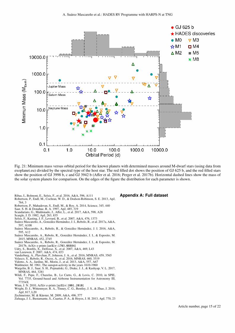
GJ 625 b is in the lower part of the Mass vs Period diagramof known planets around M-dwarf stars with measured dynamicmasses (Fig. 21). The proposed projected mass would make it thelightest planet found around an M2 star to date. Of all the knownplanets around M-dwarfs with dynamical masses determined ∼52 % are super-Earths or Earth-like planets (< 10 M⊕) at periodsshorter than 100 days. Fig. 21 points out once more the lack ofmassive planets in close orbits around M-dwarfs, only ∼ 9 %of detected planets at periods shorter than 10 days being heavierthan 10 M⊕, with only one going over 1 MJup, as expected by thecore-accretion formation model (Laughlin et al. 2004). There isalso a lack of small planets (< 3 M⊕) in close orbits (< 10 days)around early M-dwarfs (M0-M2), with GJ 3998 being the onlyone. At periods longer than 10 days on the other hand there is agreat abundance of this kind of planets.
The presence of one or more extra planets around the star GJ625 cannot yet be ruled out at longer orbital periods and smallRV amplitudes ( < 1.5 ms−1 for periods shorter than 3 years),
but finding them will not be easy. The rotation period, combinedwith the signs of differential rotation, would make difficult thedetection of low amplitude planetary signals in the range of pe-riods from 35 to 120 days, as stated at the end of Section 5. Alsoconsidering the detected magnetic cycle it would be expected tofind a RV signal at 1.5 yr or 3 yr eventually arising. The mostpromising candidates to continue searching would be very smallmass planets at very close orbits, and small mass planets in thehabitable zone of the star, at periods shorter than 30 days.
The activity induced RV variations measured both using theCCF fitting and the TERRA pipeline are not consistent with eachother. With the CCF fitting favouring a signal at 74 days, verysimilar to the ones measured in the B-,V- and R-band photome-try and in the Ca II H&K variations, while the TERRA pipelinefavours a 85 d signal closest to the signal measured in the Hα
index. Stellar induced signals are usually more complicated thanplanetary signals, and the long period and low amplitude of thesignals (∼ 1.6 ms−1), combined with their non-sinusoidal shape,could easily lead to an incorrect modelling. The spectral windowof the observation series might also be playing a part here. Theregion around 70-100 days is a complicated one, so it cannot beruled out that it is affecting the 82 and 85 days measurements. Ifwe assume that this is not the case, it could be that the changein the source of RV information (a selection of lines in the CCFvs the full spectrum in TERRA) is making the two algorithmssensitive to different active regions or even different depths ofthe stellar atmosphere. If this were the case the use of both al-gorithms for the same star could prove a very useful tool for thediagnosis of activity induced signals, maybe even for the case ofearlier spectral types (G and K-type stars). Further investigationusing data from different stars would be needed.
GJ 625 has an estimated mass of 0.3 M�, placing it closeto the theoretical limit at which a star becomes fully convec-tive. If the proposed 3 yr magnetic cycle could be confirmed itwould place GJ 625 in the small group of very small mass starswhich exhibit activity cycles despite theoretical predictions sug-gesting they should not (Chabrier & Küker 2006; Robertsonet al. 2014; Suárez Mascareño et al. 2016; Wargelin et al. 2017).The growing number of detected cycles in stars that are expectedto be fully-convective, and therefore to not have a tachocline,supports the idea that the stellar dynamo might not be confinedto the tachocline but instead distributed across the convectionzone (Wright et al. 2016).
8. Conclusions
We have analysed 151 high resolution spectra along with photo-metric observations in 4 different bands to study the presence ofplanetary companions around the M-dwarf star GJ 625 and itsstellar activity. For the study of this system, we extracted the ra-dial velocity information in two different ways, on one hand us-ing the cross correlation of the spectra with a numerical template,on the other hand by template matching the individual spectrawith a high S/N template.
We detected one significant radial-velocity signals, at a pe-riod of 14.6 d. A second one arises at 74-85 days, with differentperiods for the different algorithms. From the available photo-metric and spectroscopic information we conclude that the 14.6d signal is caused by a planet with a minimum mass of 2.82 M⊕in an orbit with a semi-major axis of 0.078 AU. The planet ison the inner edge of the habitable zone, with its mean surfacetemperature very dependent on the atmospheric parameters. Theshort period of the planet makes it a potential transiting candi-date. Following Winn (2010) we find the transit probability of GJ
Article number, page 11 of 22

A&A proofs: manuscript no. GJ625_AA_vArxiv
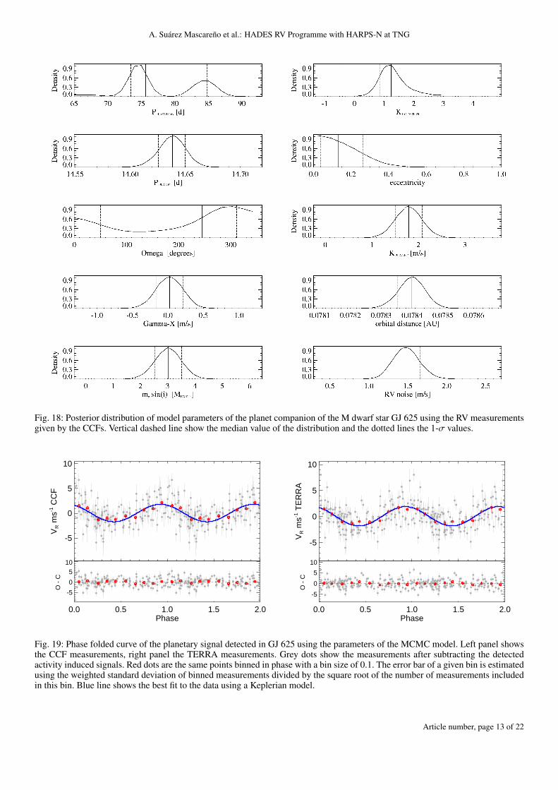
Fig. 17: Posterior distribution of model parameters of the planet companion of the M dwarf star GJ 625 using the RV measurementsgiven by the TERRA pipeline. Vertical dashed line show the median value of the distribution and the dotted lines the 1-σ values.
Table 5: MCMC parameters and uncertainties
TERRA CCFParameter Value Upper error Lower error Value Upper error Lower error PriorPplanet [d] 14.628 +0.012 −0.013 14.638 +0.012 − 0.013 10.5 - 18.5γ [ms−1 + 12850] -0.11 +0.18 −0.18 -0.07 + 0.19 − 0.20 −3.0 - +3.0e 0.13 +0.12 −0.09 0.13 + 0.13 − 0.09 0.0 - 0.99ω [deg] 343.1 +9.6 −14.8 240 + 70 − 180 0.0 - 360.0χ 0.94+ +0.026 −0.043 0.26 + 0.45 − 0.18 0.0 - 0.99Kplanet [ms−1] 1.67 +0.29 −0.29 1.79 + 0.29 − 0.30 0.0 - 3.0a [AU] 0.078361 +0.000044 −0.000046 0.078399 + 0.000042 − 0.000045 –mp sin i [MEarth] 2.82 +0.51 −0.51 3.02 +0.49 − 0.50 –
PRot [d] 84.7 + 1.3 − 1.8 76.1 + 8.9 − 3.0 65.0 - 95.0KRot [ms−1] 1.41 + 0.53 − 0.47 1.25 + 0.52 − 0.39 0.0 - 3.0
RV noise [ms−1] 1.61 +0.18 −0.18 1.48 + 0.18 − 0.17 0.0 - 3.0
625 b in the range of 1.5 - 2.5 %. Detecting the transits wouldgive a new constraining point to the mass-radius diagram andprovide further opportunity for atmospheric characterization.
The second radial-velocity signal of period 74-85 d and semiamplitude of 1.6 ms−1 is a magnetic activity induced signal re-lated to the rotation of the star. Using the photometric light
curves and the time-series of spectral indicators we concludethat the rotation period of the star is ∼ 74 days, with evidenceof differential rotation up to ∼ 85 days. We have seen that themeasured rotation period and the amplitude of the rotation in-duced signal match the expected results of Suárez Mascareñoet al. (2015, 2016, 2017b). We also found evidence for a mag-
Article number, page 12 of 22
A. Suárez Mascareño et al.: HADES RV Programme with HARPS-N at TNG
Fig. 18: Posterior distribution of model parameters of the planet companion of the M dwarf star GJ 625 using the RV measurementsgiven by the CCFs. Vertical dashed line show the median value of the distribution and the dotted lines the 1-σ values.
0.0 0.5 1.0 1.5 2.0
-5
0
5
10
VR m
s-1 C
CF
0.0 0.5 1.0 1.5 2.0Phase
-5
0
5
10
O -
C
0.0 0.5 1.0 1.5 2.0
-5
0
5
10
VR m
s-1 T
ER
RA
0.0 0.5 1.0 1.5 2.0Phase
-5
0
5
10
O -
C
Fig. 19: Phase folded curve of the planetary signal detected in GJ 625 using the parameters of the MCMC model. Left panel showsthe CCF measurements, right panel the TERRA measurements. Grey dots show the measurements after subtracting the detectedactivity induced signals. Red dots are the same points binned in phase with a bin size of 0.1. The error bar of a given bin is estimatedusing the weighted standard deviation of binned measurements divided by the square root of the number of measurements includedin this bin. Blue line shows the best fit to the data using a Keplerian model.
Article number, page 13 of 22

A&A proofs: manuscript no. GJ625_AA_vArxiv
Fig. 20: Mean surface temperature of GJ 625 b as a function ofalbedo and the fraction of radiation absorbed by the atmosphere(top panel) and change of the habitable zone as a function ofcloud coverage of the planet (bottom panel). The Earth symbolshows where it would be with an Earth-like albedo and green-house effect (top panel), and with an Earth-like cloud coverage(bottom panel).
netic cycle of ∼3 yr which would need future observations to bebetter constrained.
Acknowledgements
We thank Guillem Anglada-Escudé for distributing the lat-est version of the TERRA pipeline. This research has madeextensive use of the SIMBAD database, operated at CDS,Strasbourg, France and NASA’s Astrophysics Data System.This work has been financed by the Spanish Ministry projectMINECO AYA2014-56359-P. J.I.G.H. acknowledges financialsupport from the Spanish MINECO under the 2013 Ramón yCajal program MINECO RYC-2013-14875. A.S.M acknowl-edges financial support from the Swiss National Science Foun-dation (SNSF). M. P., I. R., J.C.M., E.H., A. R., and M.L. ac-knowledge support from the Spanish Ministry of Economy andCompetitiveness (MINECO) and the Fondo Europeo de Desar-rollo Regional (FEDER) through grant ESP2016-80435-C2-1-R. mGAPS acknowledges support from INAF trough the "Pro-getti Premiali” funding scheme of the Italian Ministry of Edu-cation, University, and Research and through the PREMIALEWOW 2013 research project. L. A. and G. M. acknowledge sup-port from the Ariel ASI-INAF agreement N. 2015-038-R.0. Theresearch leading to these results has received funding from theEuropean Union Seventh Framework Programme (FP7/ 2007-2013) under Grant Agreement No. 313014 (ETAEARTH). G.S.acknowledges financial support from “ Accordo ASI–INAF” n.2013-016-R.0 July 9, 2013.
ReferencesAffer, L., Micela, G., Damasso, M., et al. 2016, A&A, 593, A117Anglada-Escudé, G., Amado, P. J., Barnes, J., et al. 2016, Nature, 536, 437Anglada-Escudé, G. & Butler, R. P. 2012, ApJS, 200, 15Astudillo-Defru, N., Bonfils, X., Delfosse, X., et al. 2015, A&A, 575, A119Astudillo-Defru, N., Forveille, T., Bonfils, X., et al. 2017, ArXiv e-prints
[arXiv:1703.05386]
Balan, S. T. & Lahav, O. 2009, MNRAS, 394, 1936Baliunas, S. L., Donahue, R. A., Soon, W. H., et al. 1995, ApJ, 438, 269Baranne, A., Queloz, D., Mayor, M., et al. 1996, A&AS, 119, 373Berdyugina, S. V. & Järvinen, S. P. 2005, Astronomische Nachrichten, 326, 283Berdyugina, S. V. & Usoskin, I. G. 2003, A&A, 405, 1121Berta-Thompson, Z. K., Irwin, J., Charbonneau, D., et al. 2015a, Nature, 527,
204Berta-Thompson, Z. K., Irwin, J., Charbonneau, D., et al. 2015b, NAT, 527, 204Boisse, I., Bouchy, F., Hébrard, G., et al. 2011, A&A, 528, A4Bolmont, E., Selsis, F., Owen, J. E., et al. 2017, MNRAS, 464, 3728Bonfils, X., Delfosse, X., Udry, S., et al. 2013, A&A, 549, A109Bonfils, X., Mayor, M., Delfosse, X., et al. 2007, A&A, 474, 293Chabrier, G. & Küker, M. 2006, A&A, 446, 1027Cosentino, R., Lovis, C., Pepe, F., et al. 2012, in SPIE, Vol. 8446, Ground-based
and Airborne Instrumentation for Astronomy IV, 84461VCovino, E., Esposito, M., Barbieri, M., et al. 2013, A&A, 554, A28Cumming, A. 2004, MNRAS, 354, 1165Delfosse, X., Bonfils, X., Forveille, T., et al. 2013, A&A, 553, A8Dressing, C. D. & Charbonneau, D. 2013, ApJ, 767, 95Dressing, C. D., Charbonneau, D., & Newton, E. R. 2015, in AAS/Division for
Extreme Solar Systems Abstracts, Vol. 3, AAS/Division for Extreme SolarSystems Abstracts, 501.03
Endl, M., Cochran, W. D., Kürster, M., et al. 2006, ApJ, 649, 436Endl, M., Kürster, M., Els, S., Hatzes, A. P., & Cochran, W. D. 2001, A&A, 374,
675Ford, E. B. 2005, AJ, 129, 1706Ford, E. B. & Gregory, P. C. 2007, in Astronomical Society of the Pacific Con-
ference Series, Vol. 371, Statistical Challenges in Modern Astronomy IV, ed.G. J. Babu & E. D. Feigelson, 189
Gaia Collaboration, Brown, A. G. A., Vallenari, A., et al. 2016, A&A, 595, A2Gaidos, E. 2013, ApJ, 770, 90Gillon, M., Triaud, A. H. M. J., Demory, B.-O., et al. 2017, Nature, 542, 456Gomes da Silva, J., Santos, N. C., Bonfils, X., et al. 2011, A&A, 534, A30Gregory, P. C. 2005, ApJ, 631, 1198Høg, E., Fabricius, C., Makarov, V. V., et al. 2000, A&A, 355, L27Horne, J. H. & Baliunas, S. L. 1986, ApJ, 302, 757Howard, A. W., Johnson, J. A., Marcy, G. W., et al. 2009, ApJ, 696, 75Howard, A. W., Marcy, G. W., Bryson, S. T., et al. 2012, ApJS, 201, 15Howard, A. W., Marcy, G. W., Fischer, D. A., et al. 2014, ApJ, 794, 51Irwin, J., Berta-Thompson, Z. K., Charbonneau, D., Dittmann, J., & Newton,
E. R. 2015, in American Astronomical Society Meeting Abstracts, Vol. 225,American Astronomical Society Meeting Abstracts, 258.01
Jehin, E., Gillon, M., Lederer, S. M., et al. 2016, in AAS/Division for PlanetarySciences Meeting Abstracts, Vol. 48, AAS/Division for Planetary SciencesMeeting Abstracts, 302.07
Kasting, J. F., Whitmire, D. P., & Reynolds, R. T. 1993, ICARUS, 101, 108Kopparapu, R. K. 2013, ApJ, 767, L8Labadie, L., Rebolo, R., Villó, I., et al. 2011, A&A, 526, A144Laughlin, G., Bodenheimer, P., & Adams, F. C. 2004, ApJ, 612, L73Lovis, C., Dumusque, X., Santos, N. C., et al. 2011, ArXiv e-prints
[arXiv:1107.5325]Maldonado, J., Scandariato, G., Stelzer, B., et al. 2017, A&A, 598, A27Markwardt, C. B. 2009, in Astronomical Society of the Pacific Conference Se-
ries, Vol. 411, Astronomical Data Analysis Software and Systems XVIII, ed.D. A. Bohlender, D. Durand, & P. Dowler, 251
Mayor, M., Bonfils, X., Forveille, T., et al. 2009, A&A, 507, 487Mayor, M., Marmier, M., Lovis, C., et al. 2011, ArXiv e-prints
[arXiv:1109.2497]Montet, B. T., Crepp, J. R., Johnson, J. A., Howard, A. W., & Marcy, G. W. 2014,
ApJ, 781, 28Mortier, A. & Collier Cameron, A. 2017, ArXiv e-prints [arXiv:1702.03885]Moss, D. 2004, MNRAS, 352, L17Newton, E. R., Irwin, J., Charbonneau, D., Berta-Thompson, Z. K., & Dittmann,
J. A. 2016, ApJL, 821, L19Noyes, R. W., Hartmann, L. W., Baliunas, S. L., Duncan, D. K., & Vaughan,
A. H. 1984, ApJ, 279, 763Oscoz, A., Rebolo, R., López, R., et al. 2008, in Proc. SPIE, Vol. 7014, Ground-
based and Airborne Instrumentation for Astronomy II, 701447Pepe, F., Mayor, M., Delabre, B., et al. 2000, in SPIE, Vol. 4008, Optical and
IR Telescope Instrumentation and Detectors, ed. M. Iye & A. F. Moorwood,582–592
Perger, M., García-Piquer, A., Ribas, I., et al. 2017a, A&A, 598, A26Perger, M., Ribas, I., Affer, L., & Suárez-Mascareño, A. 2017b, A&APoretti, E., Boccato, C., Claudi, R., et al. 2016, Mem. Soc. Astron. Italiana, 87,
141Queloz, D., Henry, G. W., Sivan, J. P., et al. 2001, A&A, 379, 279Quirrenbach, A., Amado, P. J., Seifert, W., et al. 2012, in Proc. SPIE, Vol. 8446,
Ground-based and Airborne Instrumentation for Astronomy IV, 84460RRajpaul, V., Aigrain, S., & Roberts, S. 2016, MNRAS, 456, L6Reiners, A. 2009, A&A, 498, 853
Article number, page 14 of 22
A. Suárez Mascareño et al.: HADES RV Programme with HARPS-N at TNG
Fig. 21: Minimum mass versus orbital period for the known planets with determined masses around M-dwarf stars (using data fromexoplanet.eu) divided by the spectral type of the host star. The red filled dot shows the position of GJ 625 b, and the red filled starsshow the position of GJ 3998 b, c and GJ 3942 b (Affer et al. 2016; Perger et al. 2017b). Horizontal dashed lines show the mass ofthe solar system planets for comparison. On the edges of the figure the distribution for each parameter is shown.
Ribas, I., Bolmont, E., Selsis, F., et al. 2016, A&A, 596, A111Robertson, P., Endl, M., Cochran, W. D., & Dodson-Robinson, S. E. 2013, ApJ,
764, 3Robertson, P., Mahadevan, S., Endl, M., & Roy, A. 2014, Science, 345, 440Saar, S. H. & Donahue, R. A. 1997, ApJ, 485, 319Scandariato, G., Maldonado, J., Affer, L., et al. 2017, A&A, 598, A28Scargle, J. D. 1982, ApJ, 263, 835Selsis, F., Kasting, J. F., Levrard, B., et al. 2007, A&A, 476, 1373Suárez Mascareño, A., González Hernández, J. I., Rebolo, R., et al. 2017a, A&A,
597, A108Suárez Mascareño, A., Rebolo, R., & González Hernández, J. I. 2016, A&A,
595, A12Suárez Mascareño, A., Rebolo, R., González Hernández, J. I., & Esposito, M.
2015, MNRAS, 452, 2745Suárez Mascareño, A., Rebolo, R., González Hernández, J. I., & Esposito, M.
2017b, ArXiv e-prints [arXiv:1703.08884]Udry, S., Bonfils, X., Delfosse, X., et al. 2007, A&A, 469, L43van Leeuwen, F. 2007, A&A, 474, 653Vanderburg, A., Plavchan, P., Johnson, J. A., et al. 2016, MNRAS, 459, 3565Velasco, S., Rebolo, R., Oscoz, A., et al. 2016, MNRAS, 460, 3519Vidotto, A. A., Jardine, M., Morin, J., et al. 2013, A&A, 557, A67Waldmeier, M. 1961, The sunspot-activity in the years 1610-1960Wargelin, B. J., Saar, S. H., Pojmanski, G., Drake, J. J., & Kashyap, V. L. 2017,
MNRAS, 464, 3281Wildi, F., Pepe, F., Chazelas, B., Lo Curto, G., & Lovis, C. 2010, in SPIE,
Vol. 7735, Ground-based and Airborne Instrumentation for Astronomy III,77354X
Winn, J. N. 2010, ArXiv e-prints [arXiv:1001.2010]Wright, D. J., Wittenmyer, R. A., Tinney, C. G., Bentley, J. S., & Zhao, J. 2016,
ApJ, 817, L20Zechmeister, M. & Kürster, M. 2009, A&A, 496, 577Zuluaga, J. I., Bustamante, S., Cuartas, P. A., & Hoyos, J. H. 2013, ApJ, 770, 23
Appendix A: Full dataset
Article number, page 15 of 22

A&A proofs: manuscript no. GJ625_AA_vArxiv
Table A.1: Full available dataset. Radial velocities are given in the Barycentric Reference Frame after subtracting the secularacceleration. Radial-velocity uncertainties include photon noise, calibration and telescope related uncertainties.BJD is referenced to day 2450000, <Vr CCF> = 12850.11 ms−1, <FWHM> 3703.09 ms−1.
BJD ∆Vr CCF σ Vr CCF ∆Vr T ERRA σ Vr T ERRA ∆FWHM BIS Span SMW σ SMW Hα σ Hα
(d) (ms−1) (ms−1) (ms−1) (ms−1) (ms−1) (ms−1)6438.576 2.00 1.31 2.64 1.19 -2.48 -7.68 0.620 0.009 0.4260 0.00066440.577 -2.63 1.25 -0.22 1.25 1.77 -6.84 0.627 0.008 0.4164 0.00056441.698 -0.08 1.33 1.63 1.31 -0.82 -8.32 0.623 0.008 0.4210 0.00056442.513 -0.88 1.21 -0.83 1.22 5.56 -8.24 0.728 0.008 0.4300 0.00056443.481 -1.17 1.52 -0.33 1.34 -1.57 -4.93 0.654 0.012 0.4157 0.00086484.636 -5.47 1.65 -4.33 1.33 2.81 -11.65 0.529 0.011 0.4124 0.00086485.458 -4.32 1.30 -4.40 1.21 -2.18 -10.24 0.595 0.008 0.4137 0.00056507.464 2.71 2.10 2.98 1.90 -6.48 -12.12 0.553 0.013 0.4069 0.00096533.354 -0.90 1.29 0.67 1.25 1.38 -8.02 0.614 0.008 0.4187 0.00056534.363 -4.75 1.65 -2.98 1.38 -5.46 -7.17 0.601 0.012 0.4221 0.00086535.419 -0.21 1.45 -0.49 1.29 -0.76 -6.18 0.592 0.012 0.4141 0.00086536.475 -0.84 1.29 1.26 1.27 -2.85 -8.30 0.684 0.008 0.4143 0.00056693.714 -2.83 1.51 -1.58 1.39 0.19 -5.41 0.744 0.013 0.4199 0.00076694.738 -2.29 1.46 -1.86 1.38 1.60 -10.44 0.721 0.012 0.4175 0.00076695.707 3.72 2.04 5.27 1.52 -0.13 -6.90 0.663 0.017 0.4140 0.00106696.698 -1.52 1.53 0.97 1.30 2.95 -5.39 0.692 0.012 0.4170 0.00076697.710 1.71 1.28 3.68 1.25 3.28 -7.19 0.821 0.011 0.4309 0.00066698.711 0.93 1.61 2.22 1.37 0.84 -4.92 0.663 0.013 0.4203 0.00086700.690 -0.65 1.31 0.92 1.26 1.72 -6.98 0.792 0.011 0.4158 0.00066701.667 3.17 1.46 4.74 1.33 -5.70 -3.22 0.717 0.013 0.4161 0.00086702.662 -1.44 1.45 1.79 1.43 -4.22 -6.69 0.769 0.011 0.4278 0.00076775.629 1.08 1.75 2.53 1.39 2.65 -10.16 0.779 0.016 0.4069 0.00106783.490 3.03 1.32 3.46 1.31 5.21 -7.24 0.818 0.012 0.4229 0.00076784.494 0.99 1.30 1.62 1.20 6.69 -4.60 0.857 0.011 0.4262 0.00066798.430 -1.74 1.29 -0.87 1.22 0.89 -6.52 0.815 0.010 0.4233 0.00066799.453 0.95 1.28 1.36 1.23 -0.99 -6.34 0.833 0.011 0.4266 0.00066800.417 0.31 1.41 3.22 1.29 2.46 -5.21 0.894 0.013 0.4371 0.00076821.485 -2.71 1.84 -3.05 1.51 -7.94 -4.35 0.590 0.016 0.4217 0.00116854.495 -1.17 1.25 0.21 1.25 -1.00 -5.66 0.931 0.011 0.4235 0.00066855.484 -1.44 1.32 -0.18 1.25 -0.89 -7.25 0.746 0.011 0.4091 0.00066857.467 -0.71 1.29 0.15 1.21 3.35 -4.95 0.813 0.012 0.4049 0.00076858.436 -0.09 1.35 1.39 1.29 4.39 -7.70 0.777 0.011 0.4093 0.00066859.458 4.93 1.32 4.60 1.28 3.63 -9.58 0.761 0.010 0.4075 0.00066860.423 2.78 1.24 3.02 1.17 4.26 -6.83 0.845 0.010 0.4127 0.00066861.450 2.21 1.27 4.23 1.24 7.78 -5.48 0.994 0.011 0.4216 0.00056877.444 2.30 1.30 3.25 1.19 2.60 -8.93 0.813 0.011 0.4292 0.00066878.442 2.18 1.23 2.98 1.25 4.06 -5.39 0.781 0.010 0.4154 0.00056879.383 -1.02 1.24 -0.29 1.19 6.14 -4.11 0.889 0.012 0.4259 0.00066880.386 1.05 1.36 2.13 1.25 4.76 -3.22 0.781 0.012 0.4214 0.00076881.403 0.84 1.95 0.81 1.47 -1.91 -6.34 0.793 0.020 0.4276 0.00116892.395 1.44 1.31 2.62 1.21 -0.40 -7.09 0.736 0.011 0.4132 0.00066893.398 3.93 1.45 2.50 1.29 3.29 -6.48 0.711 0.012 0.4140 0.00076894.401 2.30 1.39 1.50 1.30 2.56 -6.94 0.716 0.010 0.4088 0.00066897.410 -2.36 1.29 -1.97 0.98 -0.59 -3.46 0.757 0.015 0.4259 0.00096898.381 -4.20 1.39 -1.51 1.07 -1.21 -7.39 0.791 0.015 0.4251 0.00096899.395 -0.69 1.26 0.34 0.98 -4.95 -0.65 0.734 0.017 0.4186 0.00106904.495 -2.25 1.01 -0.90 0.90 -2.00 -6.76 0.760 0.009 0.4263 0.00066905.388 1.03 0.99 1.21 0.94 -6.51 -4.09 0.767 0.011 0.4209 0.00066907.382 -2.05 1.02 -0.46 0.92 -10.51 -5.15 0.694 0.010 0.4182 0.00066909.380 -4.11 1.23 -2.25 1.24 -7.44 -4.52 0.707 0.009 0.4196 0.00066918.389 -3.37 1.48 -3.10 1.18 -8.96 -7.26 0.595 0.013 0.4138 0.00096920.388 -2.44 1.09 -1.45 0.93 -13.49 -10.08 0.670 0.010 0.4172 0.00076921.393 -1.43 1.78 -1.85 1.38 -15.38 -6.81 0.658 0.016 0.4167 0.00106932.342 -1.54 1.45 -1.60 1.26 -5.48 -9.18 0.706 0.016 0.4190 0.00106938.320 -1.49 1.08 0.61 0.97 -1.03 -7.88 0.779 0.012 0.4142 0.00076940.320 -0.47 1.16 -0.94 1.36 -0.26 -5.09 0.830 0.013 0.4176 0.00076942.318 1.43 0.93 1.41 0.90 4.59 -6.06 0.909 0.010 0.4208 0.0005
Article number, page 16 of 22

A. Suárez Mascareño et al.: HADES RV Programme with HARPS-N at TNG
Table A.1: Full available dataset. Radial velocities are given in the Barycentric Reference Frame after subtracting the secularacceleration. Radial-velocity uncertainties include photon noise, calibration and telescope related uncertainties.BJD is referenced to day 2450000, <Vr CCF> = 12850.11 ms−1, <FWHM> 3703.09 ms−1.
BJD ∆Vr CCF σ Vr CCF ∆Vr T ERRA σ Vr T ERRA ∆FWHM BIS Span SMW σ SMW Hα σ Hα
(d) (ms−1) (ms−1) (ms−1) (ms−1) (ms−1) (ms−1)6943.315 1.45 1.07 0.40 0.95 4.47 -5.65 0.831 0.012 0.4140 0.00067113.565 -3.73 1.63 -2.42 1.41 -7.34 -2.10 0.773 0.017 0.4062 0.00097114.622 -5.75 3.47 -3.72 2.51 -4.94 -10.36 0.769 0.034 0.4065 0.00197115.529 -2.29 1.58 -2.15 1.30 -9.84 -5.27 0.629 0.013 0.4031 0.00087116.576 -2.83 1.26 -1.73 1.18 -4.91 -5.72 0.660 0.009 0.4038 0.00057123.548 2.42 3.67 1.08 2.45 0.81 -6.15 0.607 0.032 0.4107 0.00227137.713 2.10 1.36 5.33 1.35 -6.38 -7.25 0.676 0.009 0.4073 0.00057139.674 4.80 1.44 3.90 1.29 -3.61 -5.28 0.650 0.011 0.4055 0.00077142.604 -0.34 1.36 0.45 1.25 -2.94 -3.25 0.720 0.012 0.4117 0.00077143.549 -1.32 1.53 -2.04 1.35 -1.85 -6.11 0.615 0.013 0.4071 0.00087144.543 0.95 1.52 1.87 1.35 -5.68 -7.39 0.760 0.015 0.4243 0.00097239.410 1.79 1.01 0.90 0.95 -1.23 -7.22 0.761 0.010 0.4157 0.00067240.410 5.76 1.03 6.15 0.95 0.21 -4.99 0.726 0.011 0.4135 0.00067241.407 0.71 1.30 2.84 1.09 -5.87 -9.06 0.723 0.013 0.4145 0.00087242.407 2.13 1.28 3.25 1.05 -4.76 -4.11 0.755 0.014 0.4269 0.00087249.438 -1.31 1.35 -2.59 1.19 1.21 -5.66 0.742 0.015 0.4135 0.00097251.395 -0.40 0.99 -1.04 0.87 2.22 -5.80 0.798 0.011 0.4209 0.00067260.370 -0.84 0.94 -0.84 0.90 -0.80 -4.44 0.777 0.010 0.4146 0.00067261.379 0.84 1.05 -0.59 1.06 1.46 -7.19 0.754 0.011 0.4099 0.00067262.376 -0.36 1.04 -0.47 0.92 3.59 -3.07 0.803 0.012 0.4212 0.00077263.376 1.33 1.00 1.77 0.95 3.34 -8.43 0.839 0.011 0.4176 0.00067264.375 -0.40 1.34 -0.34 1.01 7.63 -3.16 0.826 0.016 0.4247 0.00097274.359 0.22 1.16 -0.10 0.93 1.28 -5.93 0.739 0.011 0.4018 0.00077275.359 -1.41 1.43 -1.71 1.39 4.38 -6.65 0.765 0.012 0.4069 0.00077276.358 -2.44 1.05 -3.20 0.95 7.00 -6.61 0.946 0.013 0.4176 0.00077277.356 -3.46 1.02 -3.28 1.03 5.83 -2.72 0.769 0.011 0.4045 0.00067282.371 2.91 0.96 5.24 1.49 3.05 -5.72 0.757 0.010 0.4013 0.00057285.373 0.59 1.27 -0.99 1.14 4.22 -5.68 0.642 0.011 0.4093 0.00077286.357 -0.47 1.09 -0.74 0.97 -1.80 -4.13 0.685 0.011 0.4050 0.00077287.359 3.16 1.10 3.46 0.98 0.28 -5.95 0.673 0.010 0.4070 0.00077293.358 0.08 1.42 -1.26 1.32 0.14 -6.87 0.731 0.012 0.4110 0.00077296.390 2.53 1.14 3.24 1.18 -1.87 -11.83 0.664 0.008 0.4146 0.00067443.689 3.02 2.09 2.59 1.47 -1.82 -5.43 0.561 0.017 0.4027 0.00117472.703 3.78 1.57 4.04 1.39 -5.03 -7.27 0.702 0.015 0.4161 0.00097474.665 6.60 1.40 5.81 1.28 -0.61 -2.85 0.671 0.011 0.4117 0.00077502.703 -0.82 1.38 -0.55 1.36 -8.39 -6.57 0.609 0.010 0.4148 0.00077508.527 -4.00 1.11 -1.33 1.00 -2.50 -7.08 0.703 0.009 0.4204 0.00067508.659 -2.13 1.50 0.54 1.44 -2.49 -12.67 0.679 0.011 0.4170 0.00077509.550 -6.62 1.49 -7.26 1.30 -1.09 -11.35 0.756 0.012 0.4202 0.00087510.531 -3.39 1.44 -3.98 1.19 -4.10 -8.28 0.681 0.011 0.4141 0.00077513.622 -3.47 1.52 -4.33 1.31 -2.63 -7.93 0.696 0.013 0.4148 0.00087521.524 -2.78 1.46 -1.79 1.25 -4.16 -4.58 0.788 0.013 0.4094 0.00077522.497 0.28 1.42 -0.78 1.37 0.43 -5.13 0.725 0.013 0.4071 0.00077523.494 -1.30 1.84 -1.64 1.41 0.56 -7.26 0.676 0.017 0.4083 0.00107524.495 -1.60 1.76 -0.93 1.60 4.52 -9.77 0.719 0.015 0.4090 0.00097525.521 -3.43 1.62 -3.72 1.27 10.84 -9.65 0.963 0.017 0.4281 0.00097535.641 -3.44 1.38 -4.24 1.15 3.99 -11.65 0.782 0.014 0.4101 0.00087536.504 -0.46 1.32 1.46 1.02 6.61 -4.87 0.802 0.014 0.4090 0.00087537.496 -0.19 1.56 -0.35 1.23 8.41 -1.00 0.973 0.020 0.4306 0.00107537.611 0.95 1.22 -1.19 1.24 6.29 -5.58 0.881 0.013 0.4135 0.00077538.489 -0.15 1.06 -0.73 1.00 2.95 -7.15 0.860 0.010 0.4218 0.00067538.620 -0.05 1.15 -0.16 1.02 4.42 -8.91 0.839 0.010 0.4101 0.00067540.658 -2.09 1.31 0.11 1.04 3.40 -10.09 0.724 0.012 0.4062 0.00077549.591 7.97 1.35 8.69 1.25 -3.93 -11.09 0.747 0.010 0.4118 0.00077550.597 5.93 1.23 6.33 1.11 5.35 -9.50 0.727 0.009 0.4206 0.00067551.582 0.78 1.48 -0.33 1.09 -1.05 -7.63 0.614 0.012 0.4151 0.00087552.554 -0.39 1.26 0.62 1.07 -0.11 -7.40 0.632 0.011 0.4142 0.00077553.561 -2.19 1.43 -1.69 1.21 -0.30 -6.43 0.655 0.013 0.4142 0.0009
Article number, page 17 of 22

A&A proofs: manuscript no. GJ625_AA_vArxiv
Table A.1: Full available dataset. Radial velocities are given in the Barycentric Reference Frame after subtracting the secularacceleration. Radial-velocity uncertainties include photon noise, calibration and telescope related uncertainties.BJD is referenced to day 2450000, <Vr CCF> = 12850.11 ms−1, <FWHM> 3703.09 ms−1.
BJD ∆Vr CCF σ Vr CCF ∆Vr T ERRA σ Vr T ERRA ∆FWHM BIS Span SMW σ SMW Hα σ Hα
(d) (ms−1) (ms−1) (ms−1) (ms−1) (ms−1) (ms−1)7594.464 0.13 1.51 -0.26 1.35 1.00 -5.21 0.817 0.012 0.4181 0.00077596.458 0.77 1.52 -0.48 1.45 1.47 -5.79 0.761 0.014 0.4188 0.00087597.470 1.36 1.53 0.71 1.43 1.71 -10.35 0.702 0.012 0.4167 0.00077603.456 -0.63 1.36 0.19 1.32 7.67 -8.98 0.757 0.009 0.4093 0.00067604.446 -0.13 1.61 -0.43 1.43 9.40 -6.31 0.779 0.014 0.4111 0.00087606.393 4.30 1.47 1.86 1.19 10.04 -5.10 0.765 0.014 0.4124 0.00087607.474 5.68 2.20 5.39 2.23 16.25 -7.92 0.763 0.018 0.4103 0.00117608.435 0.46 1.12 -0.90 1.02 9.23 -6.53 0.802 0.011 0.4103 0.00067609.430 -1.96 3.14 -2.40 2.19 13.38 -7.73 0.817 0.030 0.4128 0.00187610.400 0.15 2.67 0.40 2.15 8.52 -7.85 0.983 0.031 0.4348 0.00167620.430 1.97 1.68 0.52 1.45 -0.40 -6.87 0.668 0.015 0.4125 0.00097621.461 1.71 2.81 -0.53 1.80 11.63 -12.30 0.436 0.018 0.4147 0.00157625.405 0.43 1.02 -0.33 1.10 -4.17 -4.94 0.815 0.011 0.4158 0.00067626.409 0.61 1.38 0.20 1.18 -5.01 -6.14 0.710 0.014 0.4111 0.00097627.403 -1.73 1.22 0.86 1.06 -6.58 -4.51 0.687 0.013 0.4175 0.00087628.406 -1.25 1.21 -1.71 1.13 -5.40 -3.69 0.814 0.011 0.4267 0.00077629.402 2.80 1.15 2.58 1.01 -0.81 -7.01 0.700 0.012 0.4179 0.00077632.404 -0.48 1.09 -0.26 0.98 -6.03 -6.18 0.744 0.011 0.4084 0.00067637.400 3.40 1.15 2.82 1.09 -5.64 -7.31 0.653 0.010 0.4186 0.00077638.385 1.80 1.16 1.54 1.12 -5.09 -8.60 0.676 0.012 0.4173 0.00087641.383 -0.89 1.00 -1.85 1.02 -5.71 -7.20 0.650 0.009 0.4261 0.00067642.382 -2.00 1.07 -2.65 1.03 -3.46 -4.29 0.627 0.010 0.4199 0.00077643.380 -1.43 1.15 -2.24 1.09 -4.58 -5.93 0.689 0.012 0.4283 0.00077645.381 -1.98 1.18 -1.15 1.16 -7.10 -8.70 0.640 0.011 0.4276 0.00077646.377 -1.07 1.14 -1.08 0.98 -5.02 -7.60 0.670 0.011 0.4161 0.0007
Article number, page 18 of 22

A. Suárez Mascareño et al.: HADES RV Programme with HARPS-N at TNG
Table A.2: EXORAP B band photometric dataset
MJD ∆mB σ mB(d) (mmag) (mmag)
6782.913 29.78 10.136784.956 30.38 10.106786.940 28.48 10.116797.895 19.68 10.146798.910 18.58 10.116801.896 30.18 10.116802.888 30.78 10.116813.872 26.58 10.106817.853 22.18 10.136830.982 9.68 10.136834.832 10.38 10.166835.832 9.68 10.116836.832 10.08 10.116839.823 0.58 10.116840.822 11.48 10.136841.822 6.38 10.206845.876 4.28 10.166851.846 20.38 10.136866.853 27.68 10.106868.852 21.48 10.107037.086 -0.92 10.117110.987 4.38 10.137112.016 -3.82 10.107113.014 1.68 10.107117.946 16.18 10.107154.924 20.78 10.077162.053 13.78 10.067165.006 31.08 10.067165.970 14.48 10.057171.845 8.18 10.067176.994 -0.22 10.077184.862 8.28 10.087196.035 2.18 10.027199.824 4.38 10.057200.864 5.28 10.047204.069 -8.42 10.047208.096 -27.02 10.087208.919 -19.02 10.057209.918 -14.72 10.037211.064 -26.02 10.057211.912 -13.12 10.037212.913 -14.62 10.047214.925 -9.82 10.037216.057 -24.32 10.037222.052 -23.82 10.087222.963 -12.92 10.057224.958 -9.02 10.047225.955 -11.42 10.037227.897 -6.52 10.047231.864 4.88 10.037232.948 6.18 10.047239.991 -16.52 10.087240.984 -12.22 10.067247.969 0.28 10.077258.951 5.28 10.067386.203 2.38 10.047398.172 -3.22 10.047416.127 -7.52 10.047417.128 -4.72 10.04
Table A.2: EXORAP B band photometric dataset (continued)
MJD ∆mB σ mB(d) (mmag) (mmag)
7419.097 -10.72 10.047424.121 -6.42 10.047425.115 -4.02 10.067437.081 -5.32 10.047439.068 -9.32 10.077440.054 -8.52 10.067443.055 1.78 10.107445.055 9.78 10.117455.091 6.38 10.057483.003 0.78 10.067483.998 0.48 10.077488.014 1.78 10.057488.995 7.68 10.057489.993 7.48 10.067490.987 -0.82 10.077491.988 1.38 10.087493.979 2.18 10.067494.957 -2.12 10.077495.949 6.88 10.107497.936 -3.12 10.067498.922 -8.52 10.107504.949 -7.32 10.057507.953 -6.12 10.057511.993 -5.12 10.057515.073 -12.12 10.087517.002 -8.52 10.117518.027 -3.92 10.057523.995 -1.02 10.057524.922 12.78 10.067545.962 -4.02 10.067546.958 1.48 10.067550.949 -2.82 10.087552.965 -7.42 10.067553.904 1.48 10.067554.847 -2.92 10.077565.945 -11.72 10.067569.959 -11.12 10.087570.957 -9.22 10.087571.956 -17.82 10.067573.957 -10.12 10.067574.957 -8.02 10.087575.990 -13.42 10.087576.989 -12.32 10.067577.987 -13.62 10.087578.987 -19.92 10.107590.945 -11.42 10.107591.949 -24.12 10.117593.977 -17.82 10.107746.197 -10.02 10.07
Article number, page 19 of 22
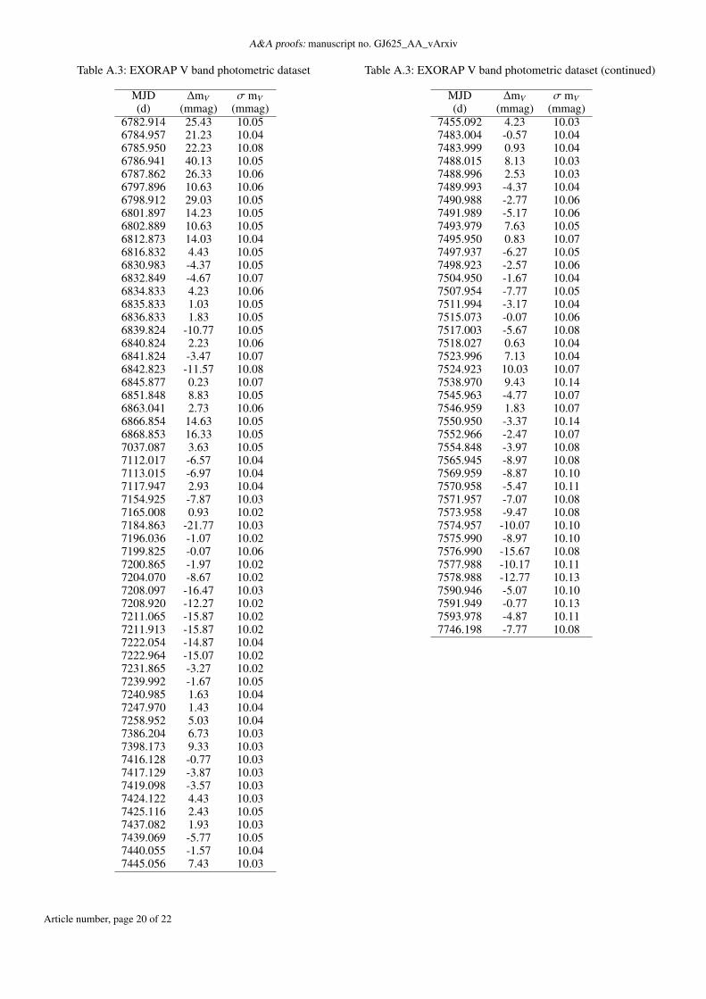
A&A proofs: manuscript no. GJ625_AA_vArxiv
Table A.3: EXORAP V band photometric dataset
MJD ∆mV σ mV(d) (mmag) (mmag)
6782.914 25.43 10.056784.957 21.23 10.046785.950 22.23 10.086786.941 40.13 10.056787.862 26.33 10.066797.896 10.63 10.066798.912 29.03 10.056801.897 14.23 10.056802.889 10.63 10.056812.873 14.03 10.046816.832 4.43 10.056830.983 -4.37 10.056832.849 -4.67 10.076834.833 4.23 10.066835.833 1.03 10.056836.833 1.83 10.056839.824 -10.77 10.056840.824 2.23 10.066841.824 -3.47 10.076842.823 -11.57 10.086845.877 0.23 10.076851.848 8.83 10.056863.041 2.73 10.066866.854 14.63 10.056868.853 16.33 10.057037.087 3.63 10.057112.017 -6.57 10.047113.015 -6.97 10.047117.947 2.93 10.047154.925 -7.87 10.037165.008 0.93 10.027184.863 -21.77 10.037196.036 -1.07 10.027199.825 -0.07 10.067200.865 -1.97 10.027204.070 -8.67 10.027208.097 -16.47 10.037208.920 -12.27 10.027211.065 -15.87 10.027211.913 -15.87 10.027222.054 -14.87 10.047222.964 -15.07 10.027231.865 -3.27 10.027239.992 -1.67 10.057240.985 1.63 10.047247.970 1.43 10.047258.952 5.03 10.047386.204 6.73 10.037398.173 9.33 10.037416.128 -0.77 10.037417.129 -3.87 10.037419.098 -3.57 10.037424.122 4.43 10.037425.116 2.43 10.057437.082 1.93 10.037439.069 -5.77 10.057440.055 -1.57 10.047445.056 7.43 10.03
Table A.3: EXORAP V band photometric dataset (continued)
MJD ∆mV σ mV(d) (mmag) (mmag)
7455.092 4.23 10.037483.004 -0.57 10.047483.999 0.93 10.047488.015 8.13 10.037488.996 2.53 10.037489.993 -4.37 10.047490.988 -2.77 10.067491.989 -5.17 10.067493.979 7.63 10.057495.950 0.83 10.077497.937 -6.27 10.057498.923 -2.57 10.067504.950 -1.67 10.047507.954 -7.77 10.057511.994 -3.17 10.047515.073 -0.07 10.067517.003 -5.67 10.087518.027 0.63 10.047523.996 7.13 10.047524.923 10.03 10.077538.970 9.43 10.147545.963 -4.77 10.077546.959 1.83 10.077550.950 -3.37 10.147552.966 -2.47 10.077554.848 -3.97 10.087565.945 -8.97 10.087569.959 -8.87 10.107570.958 -5.47 10.117571.957 -7.07 10.087573.958 -9.47 10.087574.957 -10.07 10.107575.990 -8.97 10.107576.990 -15.67 10.087577.988 -10.17 10.117578.988 -12.77 10.137590.946 -5.07 10.107591.949 -0.77 10.137593.978 -4.87 10.117746.198 -7.77 10.08
Article number, page 20 of 22

A. Suárez Mascareño et al.: HADES RV Programme with HARPS-N at TNG
Table A.4: EXORAP R band photometric dataset
MJD ∆mV σ mV(d) (mmag) (mmag)
6782.915 36.87 10.056784.957 42.47 10.046785.951 34.37 10.086786.941 44.07 10.046787.863 45.67 10.066798.912 45.77 10.056802.890 30.27 10.056830.984 21.57 10.056832.849 17.57 10.076834.834 20.47 10.086835.834 18.17 10.056839.825 17.57 10.056841.824 12.17 10.086845.878 22.17 10.076851.848 27.07 10.056863.042 9.17 10.067037.088 1.67 10.057112.017 3.17 10.037113.016 -11.23 10.047117.947 -8.23 10.037154.925 -4.53 10.037165.008 5.67 10.027184.863 -8.83 10.037196.037 -3.13 10.027199.826 -5.83 10.037200.866 -1.93 10.027204.071 -19.03 10.027208.098 -34.83 10.027211.065 -17.73 10.027222.054 -29.33 10.027231.866 -5.13 10.027239.992 -5.83 10.057240.985 -10.53 10.047247.970 -12.63 10.057258.953 -1.73 10.057386.204 -0.33 10.047398.173 0.17 10.047416.129 -14.53 10.047417.129 -10.33 10.047419.098 -8.53 10.047424.123 -9.73 10.047425.117 -9.03 10.067437.082 -0.53 10.047439.069 -4.03 10.057440.056 -3.03 10.057445.056 1.17 10.047455.093 -4.13 10.047483.004 -2.13 10.057483.999 -1.23 10.067488.016 12.77 10.047488.996 -7.33 10.047489.994 -3.53 10.057490.989 -5.03 10.067491.990 -7.73 10.067493.980 -7.13 10.057495.950 -7.33 10.067497.938 -8.43 10.057498.923 -15.43 10.057504.950 -6.03 10.047507.955 -9.93 10.04
Table A.4: EXORAP R band photometric dataset (continued)
MJD ∆mV σ mV(d) (mmag) (mmag)
7511.994 -8.33 10.047515.074 -17.83 10.067517.003 -14.53 10.087518.028 -5.63 10.047524.923 10.47 10.087538.970 -4.53 10.137545.963 -3.13 10.107546.959 0.67 10.107552.966 0.87 10.107554.848 6.37 10.137565.946 4.57 10.117569.960 -13.13 10.147570.958 -5.33 10.147571.957 -18.33 10.117573.958 -7.23 10.117574.958 -14.33 10.147575.991 -22.83 10.147576.990 -6.63 10.117578.988 0.97 10.167590.946 -4.83 10.137593.978 -13.23 10.147746.198 -8.33 10.08
Article number, page 21 of 22
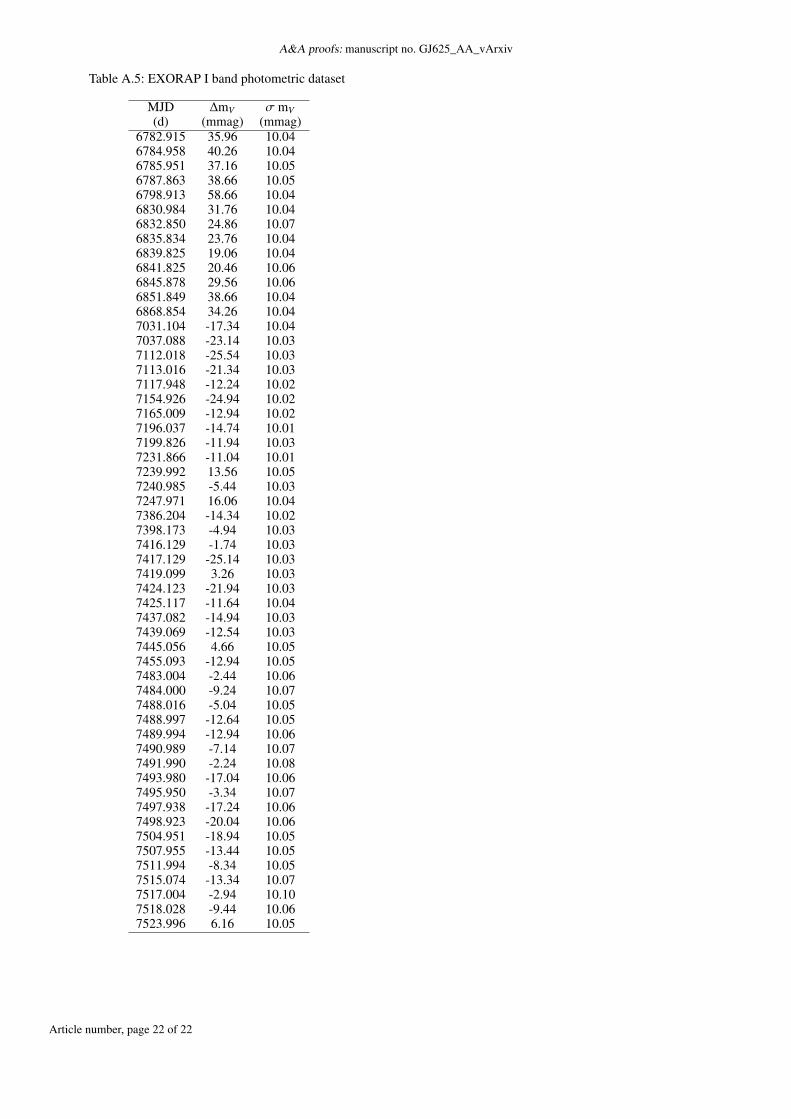
A&A proofs: manuscript no. GJ625_AA_vArxiv
Table A.5: EXORAP I band photometric dataset
MJD ∆mV σ mV(d) (mmag) (mmag)
6782.915 35.96 10.046784.958 40.26 10.046785.951 37.16 10.056787.863 38.66 10.056798.913 58.66 10.046830.984 31.76 10.046832.850 24.86 10.076835.834 23.76 10.046839.825 19.06 10.046841.825 20.46 10.066845.878 29.56 10.066851.849 38.66 10.046868.854 34.26 10.047031.104 -17.34 10.047037.088 -23.14 10.037112.018 -25.54 10.037113.016 -21.34 10.037117.948 -12.24 10.027154.926 -24.94 10.027165.009 -12.94 10.027196.037 -14.74 10.017199.826 -11.94 10.037231.866 -11.04 10.017239.992 13.56 10.057240.985 -5.44 10.037247.971 16.06 10.047386.204 -14.34 10.027398.173 -4.94 10.037416.129 -1.74 10.037417.129 -25.14 10.037419.099 3.26 10.037424.123 -21.94 10.037425.117 -11.64 10.047437.082 -14.94 10.037439.069 -12.54 10.037445.056 4.66 10.057455.093 -12.94 10.057483.004 -2.44 10.067484.000 -9.24 10.077488.016 -5.04 10.057488.997 -12.64 10.057489.994 -12.94 10.067490.989 -7.14 10.077491.990 -2.24 10.087493.980 -17.04 10.067495.950 -3.34 10.077497.938 -17.24 10.067498.923 -20.04 10.067504.951 -18.94 10.057507.955 -13.44 10.057511.994 -8.34 10.057515.074 -13.34 10.077517.004 -2.94 10.107518.028 -9.44 10.067523.996 6.16 10.05
Article number, page 22 of 22