guy yona - taurel006/vic_thesis.pdf · a thesis submitted toward the degree of ... mppt maximum...

TEL AVIV UNIVERSITY The Iby and Aladar Fleischman Faculty of Engineering

The Zandman-Slaner School of Graduate Studies

VIRTUAL INFINITE CAPACITORS

A thesis submitted toward the degree of Master of Science in Electrical and Electronic Engineering

by

Guy Yona

January 2013

TEL AVIV UNIVERSITY The Iby and Aladar Fleischman Faculty of Engineering

The Zandman-Slaner School of Graduate Studies

VIRTUAL INFINITE CAPACITORS

A thesis submitted toward the degree of Master of Science in Electrical and Electronic Engineering

by

Guy Yona

This research was carried out in the School of Electrical Engineering under the supervision of Prof. George Weiss

January 2013

ii

I dedicate this thesis to my darling wife Olga, in

grateful thanks for her patience, support and

love. I also dedicate this thesis to my loved

grandfather Zvi Porat, who taught me the love of

knowledge.

iii

Acknowledgements

First and foremost, I had both the privilege and the pleasure of working with Prof.

George Weiss. George has an admirable combination of acute mind, kindness and

perseverance. The lessons I have learnt from him during the course of the last two years

grow far beyond academic skills and knowledge. George has become truly a mentor to

me.

I am gratefully thankful to my parents Alon and Dalia, and to my wife Olga, who

enabled me to pursue my studies, through not a minute personal cost to themselves,

without whom I could not have undertaken this project.

I wish to thank the staff of the Tel-Aviv University Faculty of Engineering, and

acknowledge the generous support of the Israel Strategic Alternative Energy Foundation,

San Francisco.

iv

Abstract

We define a virtual infinite capacitor (VIC) as a nonlinear capacitor that has the

property that for an interval of the charge Q, the voltage V remains constant. We propose

a lossless approximate realization for the VIC using switches, an inductor and two

capacitors. This circuit requires a complex control algorithm that we describe. The VIC

is useful as a filter capacitor for various applications, for example power factor

compensators (PFC), as we describe. In spite of using small capacitors, the VIC can

replace a very large capacitor in applications that do not require substantial energy

storage, such as power filtering. We give simulation results for a PFC working in critical

conduction mode with a VIC for output voltage filtering, with both circuits operating in

zero-voltage-switching conditions.

v

Contents

Symbols and Abbreviations ........................................................................................... vi

List of Figures ............................................................................................................... vii

1. Introduction ................................................................................................................. 1

2. The virtual infinite capacitor ....................................................................................... 5

2.1. Nonlinear capacitors ............................................................................................. 5

2.2. Definition of a virtual infinite capacitor ............................................................... 7

3. A proposed implementation of the VIC ...................................................................... 9

3.1. The canonical switching cell ................................................................................ 9

3.2. The proposed circuit ........................................................................................... 11

3.3. Controlling the charge in a VIC ......................................................................... 12

4. Control of the VIC .................................................................................................... 16

4.1. Sliding mode control .......................................................................................... 16

4.2. The control problem of a boost converter .......................................................... 19

4.3. The proposed control algorithm ......................................................................... 22

4.4. Parameter sensitivity of the VIC ........................................................................ 25

5. An application of the VIC in a PFC .......................................................................... 29

5.1. Power Factor Compensation .............................................................................. 29


5.3. Simulation results ............................................................................................... 34

5.4. An improvement – integral sliding mode control .............................................. 39

6. Zero-voltage-switching (ZVS) of a PFC and a VIC.................................................. 41

6.1. Overview of ZVS and motivation ...................................................................... 41


6.3. Simulation results of a ZVS PFC ....................................................................... 50

6.4. ZVS implementation of the VIC ........................................................................ 53

7. Conclusion................................................................................................................. 61

8. Bibliography .............................................................................................................. 63

vi

Symbols and Abbreviations

CRM Critical Conduction Mode

ESR Equivalent Series Resistance

FCCrM Frequency Clamped Critical conduction Mode

IGBT Insulated Gate Bipolar Transistor

ISM Integral Sliding Mode

LPF Low-Pass Filter

MOS Metal-Oxide-Semiconductor

MOSFET Metal-Oxide-Semiconductor Field Effect Transistor

MPPT Maximum Power Point Tracking

MRC Multi-Resonant Converter

ODE Ordinary Differential Equation

PF Power Factor

PFC Power Factor Compensation

PI Proportional-Integral (means of control)

PV Photovoltaic

PWM Pulse Width Modulation

QSC Quasi-Square wave Converter

QSM Quasi Sliding Mode

SMC Sliding Mode Control / Sliding Mode Controller

THD Total Harmonic Distortion

VIC Virtual Infinite Capacitor

VSS Variable Structure System

ZVS Zero-Voltage Switching

vii

List of Figures

1.1 Simplified structure of a switching AC/DC power supply 1

1.2 Life expectancy of electrolytic capacitors as a function of temperature 3

2.1 � − � characteristics of a virtual infinite capacitor 7

2.2 A typical application of the VIC 8

3.1 A canonical switching cell 9

3.2 Average model of a canonical switching cell 10

3.3 Current and voltage waveforms in the canonical switching cell 10

3.4 A realization of the VIC 11

3.5 A proposed charge controller for the VIC 14

4.1 An example double integrator system with variable feedback 16

4.2 Phase trajectories of the system from Figure 4.1 17

4.3 Sliding mode regime of the system from Figure 4.1 18

4.4 Average model of the VIC 20

4.5 Plot of duty cycle dynamics (4.5) showing the instability if the VIC 21

4.6 The average switching frequency of the VIC vs. the sampling frequency 26

4.7 The RMS error of the output voltage of the VIC vs. the sampling period 26

4.8 The RMS error of the output voltage of the VIC vs. the switching frequency 27

4.9 The RMS error of the output voltage of the VIC vs. the control parameter � 28

5.1 A PFC using a boost converter with a VIC as the output capacitor 31

5.2 The waveform of the inductor current in critical conduction mode 31

5.3 The PFC from Figure 5.1 with the average model of the boost converter 33

5.4 Simulation results for a PFC boost converter using a VIC 35

viii

5.5 Simulation results for the power-up phase of the PFC boost converter 36

5.6 Simulation results for an output power change from 250W to 500W 37

5.7 Simulation results for an output power change from 500W to 250W 38

5.8 Simulation results for a PFC using a VIC with an integral sliding function 40

6.1 Waveforms of the current and voltage in a non-ZVS boost converter 44

6.2 Zero-voltage-switching version of the boost converter in a PFC 45

6.3 Waveforms of the current and voltage in a ZVS boost converter 46

6.4 Simulation results for a ZVS boost converter PFC using a VIC 51

6.5 Simulation results for the power-up phase of the ZVS PFC using a VIC 52

6.6 Simulation results for an output power change in the ZVS PFC using a VIC 53

6.7 A realization of the VIC showing the parallel capacitance of the switches 54

6.8 Average model of the VIC operating in critical mode 55

6.9 Waveforms of the current and voltage in a VIC operating in critical mode 57

6.10 Simulation results for a PFC using a VIC operating in critical mode (in ZVS) 58

6.11 Bode plot of the dependence of the output voltage error in the noise in a VIC 59

6.12 Simulation results: PFC using a VIC with the integral critical mode controller 60

7.1 � − � characteristic of a virtual "big" capacitor 62

1

1. Introduction

Most power converters require input and output filters with capacitors for the

purpose of voltage smoothing, in particular switching noise suppression. Unfortunately,

covering the low frequency range requires a large capacitance, which has three major

disadvantages: (1) low reliability; (2) large size; (3) high cost. We shall demonstrate

those disadvantages in several common power converters.

As an important example, we look at the basic structure of a switching single

phase AC/DC power supply, shown in Figure 1.1. A rectified AC voltage is passed

through a capacitive low-pass filter, which holds the voltage at a fairly constant DC level

with a ripple determined by its capacitance. Often, regulation also requires power factor

compensation (PFC), which warrants an additional circuit before the filtering, see

Chapter 5. A highly regulated low voltage, typically in the order of 3-24V, is usually

required on the DC side, hence a DC/DC converter is used to step down the voltage. For

safety reasons and the high voltage ratio, an insulated DC/DC converter topology is

generally used (such as flyback, forward, push-pull, half and full bridge topologies [45]),

which incorporates a high frequency transformer. To allow a proper functioning of the

DC/DC converter, the ripple on its input voltage �� must be constrained. The filter

capacitor, with capacitance �, must supply the load between line peaks (at twice the grid

frequency, if a full bridge rectifier is used) and allow the voltage to drop to a minimum ��. If we do not use a PFC, then the capacitance needed is

� = �� − �� , (1.1)

where � is the converter input power, � the grid frequency and �� is the minimal peak

voltage of the grid [44].

Figure 1.1: Simplified structure of a switching AC/DC power supply. The

alternating grid voltage is first rectified, then filtered by a capacitor,

converted to the required voltage and filtered again at the output side. The

PFC stage is optional.

grid connection

DC/DC converter

PFC DC

connection ��

2

A practical rule of thumb is to choose the ripple on �� to be 25-30% of the

minimum peak grid voltage. Using (1.1), we find that a typical 500W power supply

would require a 300μF capacitor (the capacitance is proportional to the power of the

converter). Only electrolytic and film capacitors are suitable for rectified grid voltages

and have high enough capacitance, with the latter being 10-20 times more expensive than

the former, and limited to about 600μF. Either kind of capacitors is very large compared

to the other components in the power supply. For example, a typical 300μF/400V

electrolytic capacitor has a diameter of 30mm and a height of 40mm (for comparison, the

dimensions of a transformer intended for the same power supply are approximately

20mm x 13mm x 11mm). The large dimensions of the filter capacitor hinder the design

of flat, small form factor power supplies, which have many uses in displays, portable

PCs, LED lighting and other applications.

We move to another example. In the growing industry of photovoltaic (PV) energy

production, the lifetime of a PV system is determined mainly by the inverter, as the

lifetime of modern PV panels surpasses 20 years, vs. an average of 5 years for the

inverter [27]. PV module inverters face harsh environmental conditions, with

temperatures up to 70ºC combined with humid of corrosive conditions, which greatly

affect the lifetime of electronic components. Aluminum electrolytic capacitors, used to

filter out the current ripple on the DC-link, are known as one of the weakest links in PV

module inverters [34]. Unlike other capacitors, electrolytic capacitors have a life

expectancy after which their equivalent series resistance (ESR) rises significantly and

they are prone to failure. The life expectancy is exceptionally susceptible to ambient

temperature, as shown in Figure 1.2. In most commercial inverters, a several hundred μF

capacitor is needed to meet the ripple requirement, and the use of film capacitors is either

impractical or very costly. Finding a way to significantly reduce the capacitance while

maintaining the same ripple or less, will facilitate the use of smaller film (instead of

electrolytic) capacitors, and would help solving the life expectancy problem of PV

module inverters. An additional advantage of using film instead of electrolytic capacitors

is a considerably smaller ESR in the former.

Many applications require both reliable and small capacitors. One example is the

module-integrated PV inverter, which is an effective PV system topology for systems

located in built-up areas. Such PV systems are prone to shading and module mismatch

that reduce the power output of the system, therefore it is useful to place a maximum

power point tracking (MPPT) converter on each panel. Often, it is more economical to

3

include also an inverter with the MPPT on each panel. These inverters have the same

reliability problem described above, and need also to be compact in order to fit into the

PV module. Similar considerations also apply to certain power supplies, especially in

aerospace systems.

Figure 1.2: Life expectancy of aluminum electrolytic capacitors as a function

of temperature. The different lines represent the common qualification tests of

commercial capacitors, determining their grade (taken from [20]).

The need for high reliability, lightweight and small form factor power converters

is growing, as renewable energy sources, electric transportation and efficient DC lighting

become more widespread. Thus, we think that it would be useful to have a high

reliability circuit that can replace a large converter capacitor. The purpose of this thesis is

to propose such a circuit. We define a virtual infinite capacitor (VIC) as a nonlinear

capacitor that has the property that for an interval of the charge Q, the voltage V remains

constant. We shall explain how such a device is useful, and how to build and control one.

In spite of using small capacitors, the VIC can replace a very large capacitor in

applications that do not require substantial energy storage. The VIC is useful as a filter

capacitor for various applications, for example power factor compensators (PFC), as we

describe. The use of much smaller capacitors instead of electrolytic capacitors

contributes to higher reliability and smaller devices. Therefore, the VIC can replace the

input or output capacitors in various power converters, where there is a significant low

frequency current flowing through the capacitor. A typical application is after the PFC

stage in single phase power supply (see Figure 1.1).

�� (°C)

4

Organization

The theoretical concept of the VIC as a type of a nonlinear capacitor is introduced

in Chapter 2. In Chapter 3 we propose and discuss a possible implementation of the VIC

using a bidirectional DC/DC converter, and the need to control its charge. In Chapter 4

we discuss the problem of controlling the VIC, propose a sliding mode controller and

discuss its parameter sensitivity. Chapter 5 contains a proposed application of the VIC as

an output capacitor of the PFC stage in a single phase power supply, including

simulation results, and demonstrates the results of an improved control using a three

dimensional sliding surface. Chapter 6 deals with ways to significantly reduce the

switching losses of the discussed implementations using zero-voltage-switching (ZVS)

techniques in both the PFC boost converter and the VIC bidirectional converter. For this

purpose, we propose and discuss a critical mode controller for the VIC.

5

2. The virtual infinite capacitor

2.1. Nonlinear capacitors

The theory of networks built from static nonlinear circuit elements was largely

developed by Leon O. Chua [4]. There are four basic types of two-terminal circuit

elements, each corresponding to a relation between two independent variables:

1. Relationship between the voltage � and the current ": a resistor ;

2. Relationship between � and the charge �: a capacitor ;

3. Relationship between " and the magnetic flux Φ: an inductor ;

4. Relationship between � and Φ: a memristor [7].

A relationship does not necessarily mean a function. For example, in a hysteresis type

relation between " and Φ , as common in an inductor, Φ cannot be expressed as a

function of " (and vice verse). Often, a circuit element can be expressed by a continuous

and piecewise smooth curve in the correct plane, one of the following "-�, �-�, "-Φ or

the �-Φ plane. Then the element is characterized by that curve, and will belong to the

corresponding type.

When a capacitor is characterized by a straight line through the origin of the �-�

plane, it is called a linear capacitor. It can be described by � = �� where � is the slope

of the straight line, or the capacitance of the capacitor. If a capacitor is characterized by

any other curve in the �-� plane, then it is a nonlinear capacitor. Nonlinear capacitors

can be found in the early references Manley and Rowe [26] and Rowe [32]. The curve of

a nonlinear capacitor can be a function by � = �(�) if it is voltage-controlled, or it can

be a function � = �(�) if it is charge-controlled. Nonlinear capacitors occur extensively

in integrated circuits, as the metal-oxide-semiconductor (MOS) capacitor is nonlinear.

Although all real capacitors demonstrate undesired nonlinearity outside of their operating

range (for instance, when exceeding their breakdown voltage), ferroelectric ceramic

capacitors also exhibit a significant nonlinear �-� curve which is used in snubbers for

power electronics switches [38]. Also, nonlinear capacitors are found in biological

systems and can be used as a model for more complex networks.

From the definition of electric current, �(�) = $ %(&)'&() , the current entering a

voltage-controlled nonlinear capacitor can be expressed by:

6

%(�) = '�(�)'� = '�(�)'� ∙ '�(�)'� = �(�)'�(�)'�

where �(�) = +,(-)+- is the dynamic capacitance (also, incremental capacitance), which

is a function of the capacitor voltage (this is a constant equal to the capacitance in the

case of a linear capacitor). In the case of a charge-controlled capacitor, we define the

dynamic capacitance � at a given point � by .� = +-(,)+, , and note that �(/) = ∞ for

1+-(,)+, 23 = 0.

In the case of a charge-controlled nonlinear capacitor (or in the equivalent case

where the � - � curve of a voltage-controlled capacitor is strictly monotonically

increasing), the energy absorbed by the circuit element during an infinitesimal change of

charge '� = %'� is '4 = �'�. In the special case of a linear capacitor, the last

equation becomes

4(�.) − 4(�)) = 5 1� �'�,((7),((8) = 12�5 '(��),((7)

,((8) = 12� :��(�.) − ��(�));, or when expressed in term of voltage, substituting � = ��,

4(�.) − 4(�)) = �2 :��(�.) − ��(�));. We note that the change of energy in the capacitor depends only on the initial and the

final values of its charge, and of its characteristic �-� curve, while being independent of

the functions �(�) or �(�). It is easy to see that a charge-controlled nonlinear capacitor is energy-conserving,

in the sense that when moving from a charge �. to another one �� > �. (charging) and

then back to �. (discharging), we get back the same energy that we have stored.

Assuming that the nonlinear capacitor cannot produce any energy, the stored energy at

any point must be positive:

5 �(�)'� ≥ 0,7) for all �. in the operating range. (2.1)

The above restriction allows to have � < 0 for some positive values of �, but we

shall not explore this possibility. The theory of synthesis of nonlinear capacitors with

prescribed �-� curves using simple components and theoretical two-port elements (i.e.

rotators, scalors, reflectors and mutators) has been investigated by Chua [4, 5] and

7

others, though remained largely impractical, due to the complexity and limitations of

realizing the proposed two-port elements (most of which are circuits that include

realizations of one or more current conveyors, which are abstract 3-terminal current

amplifiers).

2.2. Definition of a virtual infinite capacitor

In this thesis we propose a circuit that behaves like a nonlinear capacitor. While

for a usual capacitor, the dependence of the voltage � on the charge �(�) = $ %(&)'&() is

linear, the �-� plot of the proposed circuit element would have a flat region for � ∈:�ABC, �ADE; as shown in Figure 2.1.

Fig. 2.1: F-G characteristics of a virtual infinite capacitor.

For charges in the interval :�ABC, �ADE; the voltage would remain at a predefined

level �HIJ. Thus, in this interval, our circuit would be equivalent to an infinite capacitor

charged to the voltage �HIJ. A charge-controlled nonlinear capacitor for which � has a flat region, namely

+-+, = 0 for � ∈ :�ABC, �ADE;, will be called a virtual infinite capacitor (VIC). A VIC

should have an additional output through which � can be measured, allowing to keep it

in the desired range � ∈ :�ABC, �ADE;,. Indeed, this is needed because in this range �

cannot be estimated from �. In the region of interest � ∈ :�ABC, �ADE;, the dynamic

capacitance is infinite, but the amount of stored energy is of course finite and not very

large. Thus, our device is good for filtering or voltage regulation, but it is not meant for

energy storage (see also Chapter 3.3). We emphasize that the �-� plot of the VIC does

not have to look like in Figure 2.1. Indeed, outside the flat region :�ABC, �ADE; the plot

may have any shape as long as the restriction (2.1) is satisfied. It is even possible to build

VICs that have a �-� plot with hysteresis, and this may be useful, for instance, if a very

fast power-up is needed (but we do not discuss this in this work).

8

A typical application of the VIC would be to create a constant voltage �HIJ on a

load KL when the energy is coming from a variable current source %�, as shown in Figure

2.2 (which may be a simplified circuit based on Norton's theorem).

Fig. 2.2: A typical application of the VIC, stabilizing the voltage on a load.

The value �HIJ may be adjustable, and � should be measurable, as explained

before. An external charge controller (not shown in the figure) may regulate %� in the

low frequency range, such that � remains in the desired range – we describe this in

Chapter 3.3.

3. A proposed implementation of the VIC

3.1. The canonical switching c

The canonical switching cell, as defined in Kassakian

Figure 3.1, is the basic ingredient in every switched power converter.

Here, / and /M are complementary logical signals, which determine the state of the

switches. Thus, if / =implemented using any suitable high

IGBTs or a diode in the case where the current flows in only one direction (in this case,

only one of the switching device

cycle N of the canonical switching cell is defined as the proportion of time that

hence 0 O N O 1. If /

controller as explained in Chapter 4, the

the proportion of time that

external signals �P, �Q, �switchings. Equivalently,

Assuming the rate

switching frequency, an average model of the canonical switching cell can be derived.

The averages of the rapidly changing signals are:

Hence, a circuit equivalent to the average model can be obtained using controlled voltage

and current sources, as shown in Figure 3.2.

C

�P %P

%Q

9

A proposed implementation of the VIC

The canonical switching cell

The canonical switching cell, as defined in Kassakian et al. [23, Ch. 6]), shown in

Figure 3.1, is the basic ingredient in every switched power converter.

Fig. 3.1: A canonical switching cell.

are complementary logical signals, which determine the state of the

1 then �� P and if / 0 then �� Q. The switches can be

any suitable high-frequency switching device, such as MOSFETs,


switching devices can be a diode). If / is a periodic signal, the duty

he canonical switching cell is defined as the proportion of time that

is a non-periodic signal, such as produced by a sliding mode

ler as explained in Chapter 4, the instantaneous duty cycle N shall be defined as

rtion of time that / 1 over a time interval that it short enough

�R, %P, %Q, %R are practically constant in it, but it contains several

switchings. Equivalently, N is obtained from / by low-pass filtering.

Assuming the rate of change of the external signals is much slower than the


The averages of the rapidly changing signals are:

�S� N�P T �1 � N!�Q,U�P N%R,U�Q �1 � N!%R.


and current sources, as shown in Figure 3.2.

%R W �R

/

/M ��

%�P

%�Q

, Ch. 6]), shown in

are complementary logical signals, which determine the state of the

. The switches can be

frequency switching device, such as MOSFETs,


is a periodic signal, the duty

he canonical switching cell is defined as the proportion of time that / 1,

periodic signal, such as produced by a sliding mode

shall be defined as

that it short enough so that the

are practically constant in it, but it contains several

of change of the external signals is much slower than the



Fig. 3.2

Since we intend to use a circuit based on the canonical switching cell as a VIC, it

would be useful to compute the voltage ripple

of �P � �Q) on the capacitor

external impedance between

currents %P, %Q, %R and assume a constant switching frequency

flowing through the capacitor and of the voltage across it are shown in Figure 3.3. While

/ 1 (the falling slope of the capacitor voltage), we have

As we assumed that %P

Fig. 3.3: Plots showing the current flowing through the capacitor

(upper plot) and the voltage across it (lower plot).

C

�Q

�P %P

%Q

%P � %�

%P � %R �P � �Q

%P

�P � �QSSSSSSSSSS

10

3.2: An average model of a canonical switching cell.


would be useful to compute the voltage ripple Δ�� (defined as the peak-to

on the capacitor � . For the sake of this computation, we assume infinite

external impedance between �P and �Q, neglect any interference from the ripple in the

and assume a constant switching frequency 1/&. Plots of the current

apacitor and of the voltage across it are shown in Figure 3.3. While

(the falling slope of the capacitor voltage), we have

� ''� ��P � �Q! %P � %R. P � %R is constant, we obtain by integration

Δ�� %R � %P� N&.

Plots showing the current flowing through the capacitor

(upper plot) and the voltage across it (lower plot).

C%R �R

W N%R

N��P � �Q!

P

Q

�S�

U�P

U�Q

+-

�

�

�P

Q / 1

/ 0


to-peak variation

, we assume infinite

, neglect any interference from the ripple in the

. Plots of the current

apacitor and of the voltage across it are shown in Figure 3.3. While

Plots showing the current flowing through the capacitor Y

Δ��

3.2. The proposed circuit

We propose an approximate

Figure 2.1, partially shown in Figure

are omitted from the figure). This realization is only an approximation

additional undesirable effects: switching noise, switching losses and small oscillations of

the voltage�.

Fig. 3.4: An approximate realization of a

and the drivers.

measuring Z[. We recognize that the central part of the circuit in Figure 3

cell, operating as a bidirectional DC/DC converter.

period \], and the signals

sampling period. In a typical application, when the VIC is used to filter t

voltage of a power factor compensator (PFC), the current

oscillate at twice the grid frequency. Charge

transferred to the capacitor

fluctuations is much lower than the

voltage �R will vary while keeping

filtering effect. Let us denote by

when� ∈ :�ABC, �ADE;

�R,ABC cannot be chosen too small, because it would lead to the DC/DC converter

working at a high voltage ratio and hence low efficiency. Ther

why �R,ABC cannot be chosen too small, and similarly

small: this will become clear when we discuss the control of the VIC in

+

_

�

11

proposed circuit

We propose an approximate realization for the virtual infinite capacitor

partially shown in Figure 3.4 (the controller and the drivers of the switches

are omitted from the figure). This realization is only an approximation


: An approximate realization of a VIC, not showing the controller

The connections on the right side are used only for

We recognize that the central part of the circuit in Figure 3.4 is a canonical switchin

cell, operating as a bidirectional DC/DC converter. The controller works with a sampling

, and the signals /, /M ∈ ^0,1_ that control the switches are constant during each

sampling period. In a typical application, when the VIC is used to filter t

voltage of a power factor compensator (PFC), the current % (and hence the charge

oscillate at twice the grid frequency. Charge fluctuations in the range

to the capacitor �R via the converter, as long as the frequency of the

fluctuations is much lower than the controller sampling frequency

will vary while keeping � almost constant (close to �HIJ), which is the desired

Let us denote by :�R,ABC, �R,ADE; the interval in which

;. We impose that

0 ? �R,ABC ? �R,ADE ? �HIJ. cannot be chosen too small, because it would lead to the DC/DC converter

working at a high voltage ratio and hence low efficiency. There is also another reason

cannot be chosen too small, and similarly �HIJ � �R,ADE cannot be chosen too

small: this will become clear when we discuss the control of the VIC in Chapter 4

W C %R

/

%

/M �R �R

realization for the virtual infinite capacitor from

(the controller and the drivers of the switches

are omitted from the figure). This realization is only an approximation, as it exhibits


, not showing the controller

The connections on the right side are used only for

canonical switching

The controller works with a sampling

that control the switches are constant during each

sampling period. In a typical application, when the VIC is used to filter the output

(and hence the charge �) will

fluctuations in the range :�ABC, �ADE; are

he frequency of the charge

1/\] . Thus, the

), which is the desired

the interval in which �R will vary

cannot be chosen too small, because it would lead to the DC/DC converter

e is also another reason

cannot be chosen too

Chapter 4.

12

We give a brief description of the circuit operation in the various regions that

correspond to the linear segments of the plot from Figure 2.1. In the first region, when

the total charge of the system is small (e.g., during power-up), the converter creates an

almost constant ratio between its input and output voltages,

N �R� �R,ABC�HIJ . This situation corresponds to the first (left) linear segment of the plot in Figure

2.1. Thus, when � reaches the value �HIJ, then �R reaches the value �R,ABC. The charge

needed for � to reach the voltage �HIJ is �ABC. The control of the converter in the first

region can be, for example, sliding mode control or pulse width modulation (PWM) with

proportional control. The dynamic capacitance in this region is � T N��R (this is valid

for frequencies significantly lower than the resonant frequency of W and �R). The second

region corresponds to the horizontal segment (for � ∈ :�ABC, �ADE;) and this is where

we want the circuit to be most of the time, because here the dynamic capacitance is

infinite. The circuit remains in the horizontal region until �R reaches the maximum

allowable value �R,ADE . The control of the VIC in the horizontal region will be discussed

in Chapter 4. In the first two regions, the switches change their state frequently, such that

/M 1 � / (actually, small delays may have to be introduced to reduce switching losses).

The third region corresponds to the rightmost segment of the plot in Figure 2.1, when

the capacitor � is on its own, while �R remains at the constant level �R,ADE . In the third

region we have / /M 0 and the dynamic capacitance is �. This situation occurs if we

overcharge the VIC.

We note that another possible realization of the VIC with �R > �HIJ exists, by

reversing the DC/DC converter. This alternative realization allows much better

regulation of �, but the higher voltage required on �R may be a drawback for many

applications.

3.3. Controlling the charge in a VIC

First, we derive a limitation on the current flowing through the VIC in sinusoidal

regime, assuming that the VIC remains in the region � ∈ :�ABC, �ADE;. Most of the

energy stored in the VIC (if realized as in Figure 3.4) is stored in the capacitor �R. Thus,

the operating range � ∈ :�ABC, �ADE; corresponds to �R holding energy in the range

13

.��R�R,ABC� ≤ 4 ≤ .��R�R,ADE� . (3.1)

As power regulation is a typical application of the VIC, it is useful to consider a

sinusoidal input current % ") sin 2cd��, as would be the case in a PFC working in

steady state on a grid with frequency gω , ignoring the ripple current (see Section V). We

assume that � �HIJ is constant. During the first half of the period (when 2cd� ≤ e)

the VIC is storing energy, and during the second half the same energy is returned. The

amount of energy stored during the half period (the increase in the total stored energy) is

Δ4 = �5 ") sin 2cd��'� = �")cd .fghi

)

According to (3.1), we have the upper bound Δ4 O .��R�R,ADE� � .��R�R,ABC� . It

follows that in order to maintain the VIC energy within the required range, the steady

state current amplitude must satisfy:

") ≤ cd�R2� j�R,ADE� � �R,ABC� k. (3.2)

Suppose that the VIC is a part of the general circuit from Figure 2.2. As mentioned

at the end of Section I, an external charge controller usually affects ini in the low

frequency range, in order to keep � ∈ :�ABC, �ADE; , or equivalently, to keep �R ∈:�R,ABC, �R,ADE;. We give an example of a simple charge controller for the circuit in

Figure 2, which can be easily adapted to most applications.

A useful way of representing ini would be

Ulm��n! 'm�n! To�n! ∙ pq�n!, (3.3)

where a hat denotes the Laplace transformation, ' is a continuous and bounded signal, p

is the control signal and o is a low-pass filter used to limit the bandwidth of the control.

The presence of o means that the control can influence %� only in the low frequency

range, corresponding to the bandwidth of o . This corresponds to typical system

constraints, such as a unity power factor in the case of a PFC, where the control should

not influence %� at the grid frequency and its harmonics, but only at lower frequencies

(see Chapter 5). For simplicity we take o�n! ..Pr] , with & > 0.

14

The total energy stored in the VIC (neglecting the inductor) is 4 .� :�R��R T��; . In the operating region � ∈ :�ABC, �ADE; the voltage � is constant, hence

'4 �R�R'�R.

Fig. 3.5: An example of a VIC charge controller, using a PI controller to

obtain the oscillations of Gst around the mid-point of the allowed range.

The squaring block compensates the nonlinearity in the plant due to (3.4).

Equating this with '4 �'� we obtain +-u+, --u�u . The solution of this

differential equation is

�R v2��R � T �R), (3.4)

where �R) is a constant. Applying the above relation for � �ABC, we obtain that

�R) �R,ABC� � 2�ABC��R . Denoting ')��! '��! � %wx(��! and using (3.3), we also have

Ulm�n! 'm)�n! To�n! ∙ pq�n!. (3.5)

We want to control p��! such that the closed loop system is stable and for any

constant '), we have lim(→| �R ��! �R,HIJ, where

+

�R,HIJ�

�R�

o�n!

1n v2��] � T �R)

�

p

CHARGE

CONTROLLER

+

}� ~1 T 1&�n� �

+

-

% �R ') ' � %wx(

15

�R,HIJ� 12�R �R,ADE� � �R,ABC� �. The choice of �R,HIJ follows from our desire to allow a maximal dynamic range for

4 in (3.1), so that the reference voltage �R,HIJ corresponds to the midpoint of the VIC

energy range.

Introduce the tracking error � �R,HIJ� � �R�. We propose to achieve the control

objective by using a PI controller }� �1 T .r�]�, with }� > 0 and &� > 0, as shown in

Figure 4. There is a squaring block in the loop, which is meant to cancel the square root

introduced by (3.4). From the block diagram we have �l � ++( ��R�! � �-�u %, and using

(3.5) we get

n��n! � ��0! �2��R jo�n!pq�n! T 'm)�n!k �2��R �o�n!}� ~1 T 1&�n� ��n! T 'm)�n!�. Using the formula for o�n!, we obtain

��n! ��n!'m)�n! � �R2� ��n!��0!, where

��n! � �-�u n�1 T &n!&n� T n� T �-�u }�n T �-�u��r�.

The stability condition for � is &� > τ, which follows from the Routh criterion.

Since �(0) = 0, it follows that for constant ') , we have indeed lim(→| � (�) = 0 as

required. The stability of the closed loop system and the fact that �(0) = 0also implies

the following: if we assume that ') is a stationary random signal, then 4(�) =�(0)4(')) = 0. If ') is a constant plus a sinusoidal signal of frequency 2cd (e.g. in a

PFC), then � is a sinusoidal signal (attenuated by �� 2%cd�� ), so that �R� oscillates

symmetrically around �R,HIJ� .

16

4. Control of the VIC

4.1. Sliding mode control

Sliding mode control (SMC) is a method of discontinues control, where the control

signal p can only have a finite number of possible values, usually two. The application of

an appropriate control law moves the phase trajectory towards a "sliding surface", which

is a desired reduced order subspace of the system state-space. The system state will then

remain close to (or "slide" along) the sliding surface, thus maintaining a sliding mode

operation. The control signal usually changes the mode (substructure) of a Variable

Structure System (VSS), for instance, by opening or closing a switch in a switched

power converter.

Sliding mode controllers are used primarily in controlling non-linear systems,

where a conventional continuous controller is hard to implement or not robust. Vadim

Utkin, one of the originators of SMC, writes that: "the major advantage of sliding mode

is low sensitivity to plant parameter variations and disturbances which eliminates the

necessity of exact modelling. Sliding mode control enables the decoupling of the overall

system motion into independent partial components of lower dimension and, as a result,

reduces the complexity of feedback design." [42]

Fig. 4.1: The example double integrator system with variable feedback

defined in (4.1). � is a discontinuous control signal, determined by the

sliding mode control law in (4.2) (taken from [37]).

We demonstrate the principle and characteristics of sliding mode control using a

double integrator with variable feedback gain as the plant to be controlled (this example

is from Spiazzi et al. [37]). This system is described by the following equations

(illustrated in Figure 4.1):

��l. = ��,�l� = }p�.,1 (4.1)

1/s 1/s '

p

17

where p ∈ ^1,−1_ is the discontinuous control input. When p = −1 , the system is

marginally stable with eigenvalues �.,� = ±%√}. When p = 1, the system is unstable

with eigenvalues �.,� = ±√} (there exists a stable trajectory in this case, �. = −√}��,

which is extremely non-robust). The phase trajectories of the two substructures of (4.1)

are shown in Figure 4.2.

Fig. 4.2: The phase trajectories of the system from Figure 4.1. Note that

the system is unstable for all but singular starting conditions, which are

sensitive to perturbations (taken from [37]).

The control law takes the form:

�.(�� + ��.) < 0 ⟹ p = +1,�.(�� + ��.) ≥ 0 ⟹ p = −1, (4.2)

where � < √} is a control parameter. This control law divides the phase-plane into two

regions, whose boundaries are the �� axis and the line �� + ��. = 0 (see Figure 4.3).

When the state trajectory crosses from one region to another, the control signal changes,

which changes the substructure of the system and causes the state trajectory to change

course. The control law should be designed to ensure that the phase trajectory will move

towards and hit a sliding surface (here, the line �� + ��. = 0) from an arbitrary initial

condition, and that the state trajectory in the vicinity of the sliding surface does not move

away from it. These conditions are called the hitting condition and the existence

condition, respectively [8]. The motion of the state trajectory on the sliding surface is

called sliding mode [37] or sliding motion, and is completely different from the

trajectories dictated by the substructures of the VSS. Indeed, on the sliding surface we

have "infinitely fast" switching of p and the evolution of the system obeys a different

differential equation. An additional desirable property of the control law is stability,

achieved when the sliding motion is always directed towards an equilibrium point, 0 in

� = −�

substructure I

� = �

substructure II

18

our example. In any practical application the switching frequency (of the commutation

between the substructures) is of course finite, hence the state trajectory will oscillate

around the sliding surface, and this trajectory will be an approximation of the sliding

motion (this is sometimes called Quasi-Sliding-Mode, or QSM [8]).

Fig. 4.3: The sliding regime of the system from Figure 4.1, under the

control law from equation (4.2). In region I, the control signal is � = −�,

and in region II, � = �. The state trajectory shows oscillations around

the sliding surface �t + �� = � , which are present in every

implementation of SMC (taken from [37]).

Let us consider now a general non-linear system [37]:

�l = �(�, �, p) = ��P(�, �, p)��(�, �) > 0,�Q(�, �, p)��(�, �) < 0,1 where � is the state vector of the system, and the vector function � (of the same

dimension) is discontinuous on the surface � = 0, where �(�, �) is called the sliding

function. The system is in sliding mode if the state � moves on the sliding surface �(�, �) = 0. The SMC process can be divided into two phases. In the first phase, called

the reaching phase [8], the controller will drive the state trajectory to converge, or hit,

the sliding surface. This phase is possible if the hitting condition, which must be derived

for the specific problem, is satisfied. The second phase is the sliding mode operation,

during which the state trajectory stays in the vicinity of the sliding surface and moves

towards a stable equilibrium point or a desired limit cycle. This is possible if the

existence and stability conditions are satisfied, which will be discussed below.

19

The existence condition demands that the state trajectories in the two

substructures on both sides of the sliding surface must be directed towards it. In other

words, for a series � → �), where �(�, �)) = 0, we have:

�(�, �) > 0�(�, �) < 0 ⇒ lim��→�8 ∇�(�, �)) ⋅ �P(�, �, p) < 0lim��→�8 ∇�(�, �)) ⋅ �Q(�, �, p) > 0. Since �l = ∑ ¢£¢�¤ ¢�¤¢( = ∇� ⋅ �, the existence condition becomes (see also a related but not

precise formulation in [37]):

�(�, �) > 0, lim��→�8 �l(�, �) < 0�(�, �) < 0, lim��→�8 �l(�, �) > 0 ⇒ lim��→�8 sgnj�(�) ∙ �l(�)k = −1. (4.3)

Naturally, the condition sgnj� ⋅ �l k = −1 when not limited locally to the vicinity

of � = 0, is a sufficient (yet hard to accomplish) hitting condition. We give here, without

proof, another, more practical, sufficient hitting condition. Let �P, �Q steady state

vectors corresponding to the inputs pP, pQ (the two possible values of p), respectively.

The sufficient hitting condition is given by:

�(�P) < 0,�(�Q) > 0. Good references on sliding mode control are Edwards and Spurgeon [8], Young,

Utkin and Özgüner [47] and Fridman, Moreno and Iriarte [10]. Levant [25] discusses

higher order sliding modes, and Spiazzi et al [37] and Tan, Lai and Tse [37] address the

issues of SMC in DC/DC converters.

4.2. The control problem of a boost converter

Let us discuss in more detail the operation of the circuit from Figure 3.4 for � ∈ :�ABC, �ADE;. Notice that we may now regard the capacitor �R as a variable voltage

source and the circuit as a boost converter that should produce a constant output voltage �HIJ. We start by showing that the aim of keeping exactly � = �HIJ cannot be achieved,

no matter what control strategy (and switching frequency) we use. This fundamental

limitation for boost converters has been discussed also in Sira-Ramirez [36] and Ortega

et al. [31, Ch. 7].

Consider the average model of the circuit

11]). Recall that no current is flowing to the terminals on the right.

constant, we have:

where N is the short-time average of

that 0 O N O 1. Hence,

�lRThis is a second order nonlinear system with state variables

control signal N. From the equality of the two expressions for

which cannot be limited

values, and hence it must

It is known that

converter (making the voltage error small) is difficult due to the unstable zero dynamics

[31, Ch. 6]. We examine th

Figure 4.4, but this time

and we are interested in the dynamics of

variables � and %], with

�

20

Fig. 4.4: Average model of the VIC.

the average model of the circuit, shown in Figure 4.4 (following [

Recall that no current is flowing to the terminals on the right. Assuming

¦N�R�lR = %,�R T WUllR N�,�R�lR %R,1

time average of / (this is the duty-cycle if q is a

Hence,

lR %N�R ,�lR %R�R ,UllR N� � �RW . This is a second order nonlinear system with state variables �R, %R , which

. From the equality of the two expressions for �lR we get

N %%R, limited to :0,1; since %R must alternate between positive and negative

must cross zero. Thus, the precise regulation of � is not possible.

t is known that the related problem of controlling the output voltage of a boost


We examine this regulation problem using the same average model from

Figure 4.4, but this time we have a constant voltage source in place of the capacitor

we are interested in the dynamics of �. We write the state equations with the state

, with �] and % constants:

�R %R �R

W

%

C +-

N�R�lR N�

shown in Figure 4.4 (following [23, Ch.

Assuming that � is

is a PWM signal) so

which depends on the

must alternate between positive and negative

is not possible.

put voltage of a boost


regulation problem using the same average model from

n place of the capacitor �R

e write the state equations with the state

21

Ull] N� 1W � �]W ,�l �N %]� T %�.

(4.4)

Eliminating the inductor current %] from (4.4), we obtain the second order ODE

�§ � NlN �l T N�

W� � N�]W� � Nl�N %. To keep � at a desired equilibrium point � �∗ , we must have �§ �l 0 . The

resulting differential equation describes the dynamics of the duty cycle N:

Nl N�W% ��] �N�∗!. (4.5)

The equilibrium points of (4.5) are given by

N 0,N �]�∗. The equilibrium point N 0 forces �] 0 and % 0 , which is a trivial equilibrium

point. The second equilibrium point has more physical significance. Recalling that an

equilibrium point �∗ of a scalar ODE �l ©��! is asymptotically stable if ©′��!1|�¬�∗ ?0, the stability of N --∗ is dependent on the direction of the current %. For % ? 0 (which

is the case when power is transferred to the higher voltage, and it is the case half of the

time in the VIC) this equilibrium point is unstable, as seen from the plot of equation (4.5)

in Figure 4.5.

Fig. 4.5: Plot of the function from (4.5) for ® ? 0 . The nontrivial

equilibrium point is unstable.

This difficulty is present even if we linearize the equations (we obtain a zero in the

right half-plane). In the linear case, this problem has been addressed by various

techniques, including ∞H control, see for instance Naim et al. [30]. The approaches

Nl N

N --∗ 0

22

based on linearization are completely inadequate when the input voltage of the boost

converter (�R in our case) varies significantly, since the small signal assumption of the

linearization is violated. Sliding mode control of boost converters, which seems to be a

very attractive approach, has been explored by several researchers, among them [31],

Cortez et al. [6], Escobar and Sira-Ramirez [9], Gee et al. [12], Guo et al. [15], Tan, Lai

and Tse [41] and Wai and Shih [46].

4.3. The proposed control algorithm

We now introduce a sliding mode controller for our circuit from Figure 3.4,

working in the region � ∈ :�ABC, �ADE;. The state equations of this system are:

¦��l = −/ ∙ %R + %,WUllR = / ∙ � − �R,�R�lR = %R.1 (4.6)

These equations are considered only in the operating range Ω defined by

|%R| O %R,ADE,�R ∈ :�R,ABC, �R,ADE;,� > �ABC, (4.7)

where 0 < �R,ABC < �R,ADE < �ABC < �HIJ. We design a sliding mode controller which is

inspired by the one in Hijazi et al. [18], but is not the same. Indeed, the sliding function

in [14][18] (a function of two state variables) is designed for a boost converter with a

constant input voltage, while our circuit requires a modified sliding function (a function

of three state variables and the disturbance %). For an oscillating (but positive) voltage �R

and an oscillating input current i we propose to use the following sliding function:

� = �HIJ − � − �(�HIJ ∙ % − �R ∙ %R), (4.8)

where only �HIJ is constant. The sliding surface Γ is the set of all possible states

� = ±�%R�R² ∈ Ω for which �(�) = 0. The proposed sliding mode control is:

/ = �1%�� < 0,0%�� ≥ 0,1 /M = 1 − /. This control law is written in an ideal form that would lead to infinitely fast switching of / and /M. In reality the switching frequency is limited, since the controller has a finite

sampling frequency 1/\] , but we ignore this fact in our analysis, because 1/\] is

assumed to be high (for further discussion see Section 4.4).

23

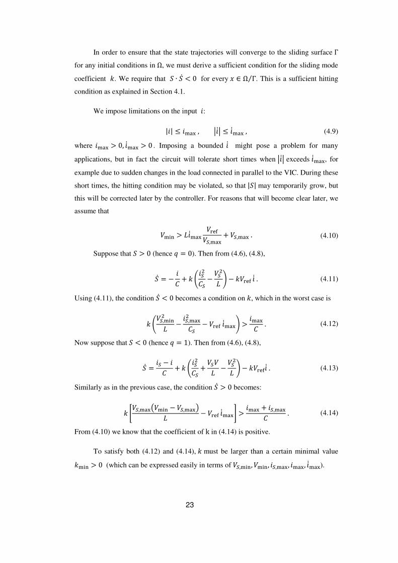
In order to ensure that the state trajectories will converge to the sliding surface Γ

for any initial conditions in Ω, we must derive a sufficient condition for the sliding mode

coefficient �. We require that � ∙ �l < 0 for every � ∈ Ω Γ⁄ . This is a sufficient hitting

condition as explained in Section 4.1.

We impose limitations on the input %: |%| O %ADE,�Ull� O UllADE, (4.9)

where %ADE > 0, UllADE > 0 . Imposing a bounded Ull might pose a problem for many

applications, but in fact the circuit will tolerate short times when �Ull� exceeds UllADE, for

example due to sudden changes in the load connected in parallel to the VIC. During these

short times, the hitting condition may be violated, so that |�| may temporarily grow, but

this will be corrected later by the controller. For reasons that will become clear later, we

assume that

�ABC > WUllADE �HIJ�R,ADE + �R,ADE. (4.10)

Suppose that � > 0 (hence / = 0). Then from (4.6), (4.8),

�l = − %� + � ´%R��R − �R�W µ − ��HIJUll. (4.11)

Using (4.11), the condition �l < 0 becomes a condition on �, which in the worst case is

� ´�R,ABC�W − %R,ADE��R − �HIJUllADEµ > %ADE� . (4.12)

Now suppose that � < 0 (hence / = 1). Then from (4.6), (4.8),

�l = %R − %� + � ´%R��R + �R�W − �R�W µ − ��HIJUll. (4.13)

Similarly as in the previous case, the condition �l > 0 becomes:

� ¶�R,ADE �ABC − �R,ADE�W − �HIJUllADE· > %ADE + %R,ADE� . (4.14)

From (4.10) we know that the coefficient of k in (4.14) is positive.

To satisfy both (4.12) and (4.14), � must be larger than a certain minimal value

�ABC > 0 (which can be expressed easily in terms of �R,ABC, �ABC, %R,ADE, %ADE, UllADE).

24

Positive values of � < �ABC can also be chosen for the sliding function if we

assume that � stays close to Γ. This is useful because a smaller � enables better output

voltage regulation, as long as the system remains stable. The condition can be expressed

by requiring that lim�→�8 sgnj�(�) ∙ �l(�)k = −1 for all �) ∈ Γ (this is the existence

condition from Section 4.1). From (4.8) we have

�(�) = 0 ⟹ % = �HIJ − � + ��R%R��HIJ . (4.15)

For � > 0, combining (4.11) and (4.15) gives the condition

��HIJ ´�R�W − %R��R + �HIJUllµ + � �R%R� > 1� (� − �HIJ). (4.16)

In a similar way, for � < 0, combining (4.13) and (4.15) gives the condition

��HIJ ´%R��R + �R(� − �R)W − �HIJUllµ + � (�HIJ − �R)%R� > 1� (�HIJ − �). (4.17)

Choosing � that satisfy both the conditions (4.16), (4.17) will fulfill the existence

condition and will ensure that the state trajectory near the sliding surface will always be

directed towards the sliding surface. Finding the range of � that will satisfy (4.16) and

(4.17) for all possible � ∈ Γ and for all Ull satisfying �Ull� < UllADE is a numerical problem

that is best handled by a computer. One usually obtains a condition of the type > �¹ABC ,

where 0 < �¹ABC < �ABC . In order to get reasonable results, we must impose an upper

bound �ADE on �, otherwise (4.16) would require an infinite �. When choosing � based

on the existence condition, we choose �ABC and �ADE close to �HIJ, to get a better (i.e.,

lower) value for �¹ABC.

Formula (4.15) imposes an upper bound for the ripple of � when � stays close to Γ

and the existence condition is satisfied. Indeed, expressing � from (4.15) and then

applying the first two constraints from (4.7) and the first constraint from (4.9) we obtain

|� − �HIJ| < � �R,ADE ∙ %R,ADE + �HIJ ∙ %ADE�. Computing �l as a function of /, the state variables, % and Ull and setting �l = 0, we

can derive the short-time average of /:

/S = W% + �� R� − L�u %R� + WUll�HIJ�W%R + ��R� (4.18)

25

By setting � = 0 and substituting (4.15) into (4.18), we get

/S = W -º»¼Q-P�-u�u�-º»¼ + �� R� − L�u %R� + WUll�HIJ�W%R + ��R� .

We note that the sliding mode control can also be achieved by an equivalent PWM

control with the duty cycle N = /S. However, we think that this equivalent PWM control

is not practical, because it requires the measurement of Ull and a complicated computation.

4.4. Parameter sensitivity of the VIC

After establishing the control of the VIC and the key requirements for its

operation, we wish to evaluate the sensitivity of the controller performance to the

changes of two important parameters: the sliding function constant �, and the sampling

period of the controller (\] from the previous section, which is actually the time between

consecutive control decisions). The first parameter was discussed at length in the

previous section. The second parameter is dependent on the implementation and requires

some explanation. The analysis done so far assumes that a change in / can occur at any

time, with unbounded switching frequency. In practice, such a controller is not possible,

and a finite frequency approximation to SMC must be observed. There are several

approaches to this approximation, including hysteresis-based control, constant ON time,

constant switching frequency, limited maximum switching frequency and constant

sampling frequency [40]. In our implementation, a constant sampling period \] is used,

and after each sampling the controller decides whether to perform a switching. Hence,

the switching frequency is variable and bounded by half the sampling frequency. The

relation between the sampling frequency 1/\] and the actual switching frequency is

shown in Figure 4.6. All the plots in this section were done with the simulation

parameters of Chapter 6 (with � = 0.002, except in Figure 4.9).

26

Fig. 4.6: The average switching frequency of the VIC vs. the sampling

frequency of the controller �/½¾. The ratio of the sampling to switching

frequency varies from 1:6.5 to 1:8.5.

Fig. 4.7: The RMS error in the output voltage G over 3 grid semi-cycles

(in red) and one semi-cycle (in blue) vs. the sampling period ½¾.

1 2 3 4 5 6 7 8 9 100

200

400

600

800

1000

1200

1400

sampling freq. (1/Ts) [MHz]

sw

itchin

g f

req.

[kH

z]

0 0.1 0.2 0.3 0.4 0.5 0.6 0.7 0.8 0.9 10

0.5

1

1.5

2

2.5

3

3.5

Ts [usec]

Vc e

rror

- rm

s

27


(in red) and one semi-cycle (in blue) vs. the switching frequency of the

VIC.

Since we wish to evaluate the performance of the VIC, we chose the RMS error of

the output voltage �HIJ − � as a simple assessment measure. We have calculated this

value over three semi-cycles of the grid (30ms, the red line in Figures 4.7-4.9) and over

one semi-cycle (10ms, the blue line in Figures 4.7-4.9), when the circuit was in steady

state. High sampling frequency calculations over 3 semi-cycles are not shown due to

simulation limitations. In Figure 4.7 we observe the almost linear decrease of the RMS

error with the shortening of the sampling period \] . Figure 4.8 shows the same

phenomenon, with respect to the switching frequency (which relates to \] via the plot in

Figure 4.6). This plot has practical importance, since the power losses of the VIC are

linearly related to the switching frequency in our implementation (although this can be

amended in a zero voltage switching implementation of the same circuit).

The dependence of the RMS voltage error on the sliding coefficient � is shown in

Figure 4.9. As expected, lower � causes the voltage error to decrease, since the term �HIJ − � in the sliding function from (4.8) becomes more dominant. However, we can

only decrease � down to a certain limit, set by the hitting and existence conditions.

0 200 400 600 800 1000 1200 14000

0.5

1

1.5

2

2.5

3

switching freq. [kHz]

Vc e

rror

- rm

s

28


(in red) and one semi-cycle (in blue) vs. the sliding coefficient ¿ defined

in (4.8). The vertical line represents the calculated minimal ¿ that fulfils

the hitting and existence conditions, at a sampling frequency of 2MHz.

0 1 2 3 4 5 6 7 8

x 10-3

0.5

1

1.5

2

2.5

3

3.5

4

k

Vc e

rror

- rm

s

29

5. An application of the VIC in a PFC

5.1. Power Factor Compensation

The power factor (PF) is defined as the ratio between the active power and the

apparent power of a system. If the current % and voltage À are periodic with period \, and

%, À ∈ ℒ�:0, \), then the active power is defined by ⟨À, %⟩ = 7Ä $ À(�)%(�)'�Å) (their inner

product in ℒ�:0, \) ), and the apparent power is defined by ‖À‖‖%‖ [11]. Hence,

PF = ⟨À, %⟩‖À‖‖%‖. When the voltage and the current are both purely sinusoidal, the PF is equal to the

cosine of the phase angle È between them. For sinusoidal voltage and non-sinusoidal

current, we define ". as the fundamental component of the current, and "É�] as the RMS

value of the current [1]. The PF depends of both the distortion factor of the waveform

(defined as "./"É�]) and the displacement factor related to the phase angle (��nÈ, where È is the phase difference between the fundamental component of the current and the

voltage waveform), in the form

PF = "."É�] ��nÈ. There are several reasons to seek a close to unity PF. First, the conduction losses in the

grid depend on the current, which is proportional to the apparent power. Since only

active power is used by the load, a PF < 1 will cause power losses due to the reactive

power flowing through the grid. In addition, harmonics caused by the waveform

distortion may disrupt other devices connected to the grid. The purpose of power factor

compensation (PFC) is to minimize the input current distortion factor, and to minimize

the phase difference between the voltage and current waves. This process is also called

power factor correction [1] or power factor conditioning [33] (each abbreviated as PFC).

As in most power supplies the periods of the current and voltage waveforms are

the same, and the peaks of the current coincide with the peaks of the voltage, the

displacement factor is close to unity. Hence, the task of PFC is reduced to eliminating the

higher order harmonics of the input current. The PF can thus be approximated by

30

PF ≈ "."É�] = v 11 + THD� , where THD is the "total harmonic distortion", which is the quadratic sum of amplitudes

of the unwanted harmonics over the squared amplitude of the fundamental harmonic

[32]. Hence, an equivalent desirable quality of a PFC would be a THD close to zero.

Several standards have been established to limit the harmonic content of the input

current of a power supply, the most common of them is EN61000-3-2 set by the

European Union in 2001. Passive PFC circuits (built from transformers, diode and

passive circuit elements) usually do not meet the standard criteria under a wide range of

loads and for applications with higher power than approximately 400W [16]. In addition,

passive PFC circuits require large and heavy magnetics. For this reason, an active PFC

circuit is usually implemented in modern power supplies. Rectifier bridges and boost

converters are most commonly used in active PFC, mostly due to their easy

implementation and good performance [1].

There are several approaches to building a PFC based on boost converters, among

them are critical conduction mode, continuous conduction mode, frequency clamped

critical conduction mode and discontinuous conduction mode boost converters.

Topologies of two boost stages are used in interleaved PFCs (common in low-profile

form factor converters) where two stages operate out-of-phase in order to reduce the

current ripple, and in bridgeless PFCs [32]. A myriad of other PFC topologies have been

proposed in the literature, for various applications and with diverse properties.


The performance of the VIC has been examined in a typical application as the

output capacitor of a boost converter used in a PFC, shown in Figure 5.1. For the boost

converter in a PFC there are two control objectives, namely: (1) attaining a nearly

constant output voltage� = �HIJ; (2) keeping the (short-time) average value of the input

current %d nearly proportional to the input voltage pd = Î sin(c�) , thus obtaining a

close to unity power factor.

There are several methods to build a PFC boost converter in continuous or

discontinuous conduction modes. The boost converter depicted here operates in the

critical conduction mode (CRM), also called border-line mode, as described in Gotfryd

[13] and in Lai and Chen [24]. In the CRM operation, each current pulse of %L has the

31

form shown in Figure 5.2. During 0 O � < �w in each pulse, the switch will be closed

and the inductor current %L will rise. During �w O � < \ the switch will be open and the

energy in the inductor will be released to the load and the VIC, causing %L to fall to zero,

Fig. 5.1: A PFC using a boost converter with a VIC as the output capacitor. Note that

the voltage Gs is measured, which is equivalent to measuring F as in Figure 2. The

internal sliding-mode controller of the VIC is not shown.

since � > pÉ = �pd�. When %L = 0 is detected, the switch will close again, starting the

next triangular pulse. Note that the switching frequency 1 \⁄ (which is variable) should

be much greater than the grid frequency. The average current in a triangle is

UlLÏ = pÉ2WÐ �w. (5.1)

Thus, to create an average current that is proportional to pÉ, we hold �w constant

during each semi-cycle of the grid (from one zero crossing of the grid to the next). Then

(according to (5.1)) the boost converter is seen from the grid like a resistor with

resistance �LÑ(Ò� , which is a desirable behavior.

Fig. 5.2: The waveform of the inductor current, as required for critical conduction mode.

%Ó

%Ó%L

%L

CRITICAL-MODE

CONTROLLER

%d pÉ

pÉ%wx(

%wx(% %

WÐ �

K �R �HIJ /Ð ��

�w %wx(

pd AC

LINE

VIC

��

%L

pÉWÐ �w

�w \ �

32

The diode is conducting only when the switch is open, hence its current %Ó

corresponds to the descending part of %L in Figure 5.2 (for �w O � < \), and %Ó = 0

otherwise. The average current of the diode is

UlÓÏ = 1\ (\ − �w) pÉ2WÐ �w. (5.2)

From elementary considerations we have −�w = xÔ-QxÔ �w , from where \ =--QxÔ �w. Substituting this into (5.2) we obtain the (short-time) average current of the

diode:

UlÓÏ = pÉ��w2WÐ�. (5.3)

The expressions (5.1), (5.3) enable us to obtain an average model of the boost

converter using a resistor and a current source that both depend on �w, as shown in

Figure 5.3.

The current flowing into the VIC is % = %Ó − %wx( . This current is fluctuating at

twice the grid frequency, and is linearly dependent on �w. We recall that the purpose of

the VIC is to hold V constant. Thus, keeping � in the region � ∈ :�ABC, �ADE; (which is

equivalent to keeping �R ∈ :�R,ABC, �R,ADE;) involves regulating �w using a variation of

the charge controller presented in Chapter 3. The value �w that the boost converter

receives is updated when the grid voltage crosses zero, hence at twice the grid frequency,

because �w should be constant in each semi-cycle to guarantee a nice sinusoidal shape

for %d . In addition, a feed-forward term from %wx( is used to improve the transient

response to changes in the load:

�w(n) = o(n) ∙ pq(n) + }Ulmwx((n), (5.4)

where p is the output of the PI controller, as in Figure 3.5, and } is the feed-forward

gain:

} = 4WÐ�HIJpd,ADE� , (5.5)

where pd,ADE is the amplitude of the grid voltage. This gain is derived from the steady-

state criterion for zero energy change during one grid semi-cycle. Indeed, integrating

(5.3) and a constant %wx( over one grid semi-cycle �0, ÕÖi� we obtain

pd,ADE� �w2WÐ� 5 sin� cd��'�Õ/Öi) = %wx( ecd.

33

Expressing from here �w, we obtain the factor } from (5.5).

Fig. 5.3: The PFC from Figure 5.1 with the average model of the boost converter.

The VIC charge controller affects both the PFC input current and the VIC input

current via ×ØÙ. Since Y®Ù is small, the circuit looks from the grid like a resistor

with resistance tÚÛ×ØÙ . Note the similarity of the right side of this circuit to the circuit

in Figure 2.

The load changes are supposed to be rare events (when a sudden change in the

load occurs, the first priority is to maintain a constant �, even at the price of temporarily

causing a distortion in %d). The feed-forward term may instantaneously affect �w, thus

violating the PFC objective of sinusoidal %d , in case the VIC does not have enough

energy reserve. The internal sliding mode controller of the VIC is not shown in Figures

5.1 and 5.3.

Finally, we discuss the power-up process of the converter. The circuit shown in

Figure 5.3 must be connected to the grid at a proper time, where �pd� ∈ :pABC, pADE; . The upper limit pADE is required in order to limit the in-rush current to the circuit at the

time of connection. The maximal allowed in-rush current is determined by the properties

of the switching components and the design specifications, and its dependence on pADE

is complex and depends on the exact realization of the VIC. When the circuit is

connected below a certain lower limit pABC, a somewhat more complicated power-up

algorithm is required to deal with the slowly charging VIC (which causes the problem of

the descending inductor current, described below, to be more pronounced). In order to

comply with these requirements, a mechanism that senses the phase of the grid and

connects the circuit at a certain phase must be incorporated in the converter. There are

� %Ó

K

%L

��

VIC CHARGE

CONTROLLER

~ AC

LINE

%wx( �w

%d pÉ %wx(

VIC

�HIJ �R

% pd

pÉ��w2WÐ� 2WÐ�w

34

several methods to realize this mechanism, and its realization is outside the scope of this

work, as are the algorithms for low-voltage (< pABC) power-up. We have found by

simulations that connecting our proposed circuit at a phase angle in the range 5° − 15° results in a stable power-up with a in-rush current less than 20A, which is acceptable for

most designs of 500W power supplies.

During power-up, there may be episodes where the slope of the descending

inductor current (as shown in Figure 5.2) xÔQ-LÑ is too low, and the rising pÉ may cause

the inductor current not to reach zero before changing the sign of the slope. To prevent

such episodes from damaging the power-up process, a protective logic should be

incorporated in the control of the boost converter. A proposed logic is to close the switch

of the boost converter when the inductor current starts rising (when supposed to be

descending), in addition to the case when %L hits zero. This would cause a secondary in-

rush current which will charge the VIC and the boost converter will resume normal

operation right afterwards as the descending slope of the inductor current will be steeper.

This logic should allow this additional trigger only when the inductor current is below a

certain limit ( xÔLÑ �w , either measured or calculated, can be used as a reference),

otherwise accidental activations of the switch would cause the current to rise on

undesired instances.

Since the VIC has no charge to begin with, it will operate in the first region (as

described in Section 3.2) until �] reaches �£,ADE . In our proposed controller, this is

implemented using PWM with a duty cycle of -u,ÝÞß-º»¼ . The feed-forward term of the

charge controller will provide the initial �w value for the control of the boost converter.

An initial value for the integrator in the PI charge controller should be set, in order to

avoid an overshoot in the input current subsequent to the power-up.

5.3. Simulation results

The VIC performance in the circuit from Figure 5.1 has been examined by

MATLAB simulations using the SimPowerSystems toolbox. The parameters of the VIC

(shown in Figure 3.4 and the sliding function (4.8)) are � = 0.002, � = 4μ©, �R =40μFand W = 60μH. From (4.12) and (4.14) we get �ABC ≈ 0.008 (this value strongly

depends on �ABC, which is chosen as �ABC = 395V ) and from (4.16) and (4.17) we get �¹ABC ≈ 0.002 (using 398 < � < 402). The sampling frequency of the VIC controller is

2MHz. The parameters of the VIC charge controller (shown in Figure 4) are }� = 2 ×

35

10Q.� , &� = 40ms , the initial value of the integrator is −0.05μs and the cut-off

frequency of the LPF is 10Hz ( o(n) = ..Pr] where & = 15.9ms). The boost converter

circuit parameters (shown in Figure 5.1) are �HIJ = 400V,K = 320Ω (thus, the power is

500W), WÐ = 60μH and �� = 100nF. The grid voltage pd has the amplitude pd,ADE =340V and the frequency Hz50 . The results are shown in Figure 5.4.

Fig. 5.4: Simulation results for a PFC boost converter using a VIC. Three grid

cycles are shown in steady state operation. All the signals shown, except for the

last (d), are filtered via a low-pass filter with a cut-off frequency of 1KHz, to

eliminate the ripple noise of the boost converter. (a) the converter input current ®ä; (b) the VIC input current ® (c) the voltage error Gåæç − G; (d) the VIC inner

capacitor voltage Gs, used as a measure of F.

0.5 0.51 0.52 0.53 0.54 0.55 0.56-4

-2

0

2

4

time [sec]

i in [

A]

0.5 0.51 0.52 0.53 0.54 0.55 0.56

-1

0

1

time [sec]

i [A

]

0.5 0.51 0.52 0.53 0.54 0.55 0.56

0

1

2

time [sec]

Verr

or [

V]

0.5 0.51 0.52 0.53 0.54 0.55 0.56100

200

300

400

time [sec]

VS [

V]

(a)

(b)

(c)

(d)

36

Fig. 5.5: Simulation results for the power-up phase of the PFC boost converter

using a VIC. Only the first semi-cycle of the grid voltage is shown here. (a) the

converter input current ®ä; (b) the VIC input current ® (c) the output voltage G;

(d) the VIC inner capacitor voltage Gs, used as a measure of F.

The calculated total harmonic distortion (THD) of the input current %d (in the

range up to 4KHz) is less than 0.7%. (the signal %d was passed through an LPF prior to

THD calculation, as most standards take into account only the first 40 harmonics of the

grid frequency in THD calculation). The low frequency voltage ripple seen in Figure

5.4(c) is 1.63V. The capacitance of a conventional capacitor, if used to achieve the same

output voltage ripple instead of the VIC, would have been � = ��-��Ö = �.è�..é�∙�Õ∙.)) ≈2.65mF, more than 65 times larger than �R (we have denoted by %�� the peak-to-peak

variation of % , as observed in Figure 5.4(b), and similarly �� is the peak-to-peak

variation of �). This ratio of 65 could be increased significantly if the DC/DC converter

were reversed, as mentioned in Chapter 3. Another way of greatly increasing this ratio

0 0.002 0.004 0.006 0.008 0.01

0

5

10

15

time [sec]

i in [A

]

0 0.002 0.004 0.006 0.008 0.01

-1

0

1

2

3

time [sec]

i [A

]

0 0.002 0.004 0.006 0.008 0.010

200

400

time [sec]

V [V

]

0 0.002 0.004 0.006 0.008 0.010

200

400

time [sec]

VS [V

]

(a)

(b)

(c)

(d)

37

(hence, lowering the ripple significantly) is by using more complex sliding functions in

the controller of the VIC is portrayed in the next section.

The power-up process of the converter is shown in Figure 5.5. Several episodes of

in-rush current occur in the first 2 milliseconds, for reasons explained in the previous

Section. In order to prevent the secondary in-rush current episodes, a sufficient charge

would have to be absorbed by the VIC during the initial in-rush current. This would

require connecting the circuit to the grid during the peak voltage, and applying an in-rush

current in order of 100A. An in-rush current of this magnitude would require less-than-

optimal switching components, and would render the circuit impractical.

Fig. 5.6: Simulation results for an output power change from 250W to 500W in a

PFC boost converter using a VIC. Three grid cycles are shown and the power

change occurs at 0.525 sec. The signals (a), (c), (d) are filtered via a low-pass

filter with a cut-off frequency of 1KHz, to eliminate the ripple noise of the boost

converter. (a) the converter input current ®ä; (b) the converter output current

®Ø�× ; (c) the VIC input current ®; (d) the voltage error Gåæç − G; (e) the VIC

inner capacitor voltage Gs, used as a measure of F.

0.5 0.51 0.52 0.53 0.54 0.55 0.56-4-2024

time [sec]

i g [

A]

0.5 0.51 0.52 0.53 0.54 0.55 0.560

0.5

1

1.5

time [sec]

i out [

A]

0.5 0.51 0.52 0.53 0.54 0.55 0.56

-1

0

1

time [sec]

i [A

]

0.5 0.51 0.52 0.53 0.54 0.55 0.56

0

1

2

time [sec]

Verr

or [

V]

0.5 0.51 0.52 0.53 0.54 0.55 0.56100

200

300

400

time [sec]

VS [

V]

(a)

(b)

(c)

(d)

(e)

38

The circuit does not exhibit PFC properties during the power-up stage. Since �w is

not constant during the power-up phase, the shape of the input current is not sinusoidal.

Starting from the second grid semi-cycle, �w will be set constant during each semi-

cycle, to allow a small THD. As described in Section 3.2, in the first region of operation

of the VIC (when the charge is less than ��), the VIC operates at a constant PWM

duty cycle N = -u,ÝÞß-º»¼ . Since �R.ABC = 100�, the duty cycle would be N = 25%. The

VIC enters the second region when � = 400�, which would correspond to �R ≥ �R,ABC.

Fig. 5.7: Simulation results for an output power change from 500W to 250W in a

PFC boost converter using a VIC. Three grid cycles are shown and the power

change occurs at 0.525 sec. The meaning of all the signals is as in Figure 5.6.

0.5 0.51 0.52 0.53 0.54 0.55 0.56-4-2024

time [sec]

i g [

A]

0.5 0.51 0.52 0.53 0.54 0.55 0.560

0.5

1

1.5

time [sec]

i ou

t [A

]

0.5 0.51 0.52 0.53 0.54 0.55 0.56

-1

0

1

time [sec]

i [A

]

0.5 0.51 0.52 0.53 0.54 0.55 0.56

0

1

2

time [sec]

Verr

or [

V]

0.5 0.51 0.52 0.53 0.54 0.55 0.56100

200

300

400

time [sec]

VS [

V]

(a)

(b)

(c)

(d)

(e)

39

Figures 5.6 and 5.7 demonstrate the stability of the output voltage during increases

or decreases of the output power, respectively. Upon reaching stability, as in Figure 5.4,

the load power changes at 0.525 seconds from 250W to 500W or vice versa. The input

current during the semi-cycle in which the power change occurs does not keep a

sinusoidal form, as �w must be changed in order to keep the VIC within the flat

operating region, as described in the previous section.

5.4. An improvement – integral sliding mode control

As we have seen, small perturbations of the output voltage � still remain in a PFC

regulated by the VIC. Since the VIC is a third-order system (equation (4.6)), and the

sliding mode controller is a second-order controller (equation (4.8)), we can try

improving the steady state performance by increasing the order of the controller. This

practice is advised in [10, Ch. 1] and in practical design guides such as [40], especially if

a fixed-frequency SMC is employed (which is the case in our implementation). This kind

of full order SMC is called Integral Sliding Mode (ISM) by Utkin and Shi [43] and in

[10, Ch. 1], but we do not follow their approach, since it requires a non-singular state

dependent input matrix, which is not our case (see (4.6)). Instead, we add a simple

integrator of the output voltage error to the sliding function �(�) (following [40]). The

improved sliding function will be

� = �HIJ − � − �(�HIJ ∙ % − �R ∙ %R) + �ì5 (�HIJ − �)'&() , (5.6)

where �ì > 0 is a second sliding coefficient. Since the implementation of the controller

is discrete, the integral is replaced by an appropriate summation.

As a result of the increased order, the existence condition of the sliding mode will

become a complex relation between � and �ì. Although it is possible to formulate this

relation analytically and use numerical methods to find the domain where the existence

condition holds, it is more practical to use the � appropriate for the second order sliding

function (4.8), and a small �ì that would not greatly influence the existence condition.

The hitting condition is not a concern in our implementation, since the reaching phase is

done using a constant PWM and not SMC, as explained in Section 5.2.

The performance of the VIC with the improved sliding function (5.6) is shown in

Figure 5.8. In this simulation, the sliding coefficients were � = 0.008, �ì = 200,000 (a

40

discrete form of the integration in (5.6) was implemented, using the Euler backward

method, i.e., í = íQ. + �îÅ (�HIJ − �) where í is the integration variable, and \] is the

sampling time). All other parameters were as in the previous section. As seen in the

simulation results, this controller indeed provides a significant improvement in the

steady state error, with a low-frequency output voltage ripple of about 50mV, in

comparison to 1.63V using the sliding function (4.6). The THD of %d is not changed by

much, with a value of 0.72%.

Fig. 5.8: Simulation results for a PFC boost converter using a VIC with the

improved full order sliding function (5.6). Three grid cycles are shown in steady

state operation. The signals (except Gs ) pass through an LPF with cut-off

frequency of 1kHz. This filter is insufficient to smooth he signal GæååØå = Gïðñ − G

in this scale, yet it is evident that the low frequency ripple is in order of 50mV.

The meaning of all the signals is as in Figure 5.4.

0.5 0.51 0.52 0.53 0.54 0.55 0.56-4

-2

0

2

4

time [sec]

i g [

A]

0.5 0.51 0.52 0.53 0.54 0.55 0.56

-1

0

1

2

time [sec]

i [A

]

0.5 0.51 0.52 0.53 0.54 0.55 0.56-0.05

0

0.05

time [sec]

Verr

or [

V]

0.5 0.51 0.52 0.53 0.54 0.55 0.56100

200

300

400

time [sec]

VS [

V]

(a)

(b)

(c)

(d)

41

6. Zero-voltage-switching (ZVS) in a PFC and a VIC

6.1. Overview of ZVS and motivation

Much of the power losses in a switched-mode power supply are due to the high-

frequency switching of the MOSFET in the PFC boost converter. This is demonstrated

by an estimation of the boost converter switching losses in our example circuit. Due to

the relatively small inductor chosen for our circuit, the average switching frequency is

high, about 430kHz. The method of power losses calculation is portrayed in [14], and

the switching component used in this calculation are the MOSFET IPP60R250CP and

the Schottky diode IDH10G65C5 by Infineon [21], [22]. This MOSFET was chosen to

have fast switching times and a small output capacitance. A silicon-carbide Schottky

diode was chosen in order to avoid the reverse recovery time of p-n junction diodes,

which is in the order of 100ns. Commonly, the most prominent factors contributing to the switching losses are:

(1) the power lost during the overlapping of the MOSFET current curve and the voltage

across it during transition, (2) the dissipation of the charge stored in the parasitic parallel

capacitance of the MOSFET during switching on, and (3) the dissipation of the reverse

recovery charge in each diode (with body diodes or switching diodes present in the

circuit) due to recombination of the minority carriers in the diode when it is turned off, or

in the case of a Schottky diode, which does not possess the reverse recovery effect,

dissipation of the charge stored in the parallel capacitance when the diode is turned on.

In the case of critical conduction mode switching, the MOSFET is switched on

when the current reaches zero. Hence, in each switching cycle the energy lost in the

switching on process is the energy stored in the parasitic parallel capacitance �w]] =0.5nF [21] alone, hence

4w = 12�w]]��. The energy lost during switching off of the MOSFET is

4wòò = 5 pÓR(�)%ÓR(�)'�(ÔóP(ô)

+ .��+� = %LÝõö� �Éx + �ò2 + .��+�, (6.1)

where: %LÝõö ≈ 2%d is the maximum inductor current in the cycle; �ò = 12nsec is the

current fall time of the MOSFET [21]; �Éx is the rise time of the voltage and �+ = 15nC

42

is the charge stored in the parallel capacitance of the diode [22]. The gate current

%ù = − -�úûüýûóþ� must discharge the gate-drain capacitance, where Kù = 1.3Ω is the gate

resistance and ��(��x = 5V is the gate Miller plateau voltage [14]. Hence,

�Éx = �ùÓ�òò�Kù��(��x , (6.2)

where �ùÓ�òò ≈ 350pF is the effective gate-drain capacitance, estimated from the

�ÓR − �ùÓ diagram [21].

Substituting (6.2) into (6.1), multiplying by the switching frequency �R� and

averaging �%d� over one grid period to achieve an average power loss, we obtain:

�R� = �R�(4w + 4wòò) = 12�R�� ¶�w]]� + �+ + 2Ud� ´�ò + �ùÓ�òò�Kù��(��x µ·. (6.3)

The average of the absolute value input current of the circuit in Chapter 5, when

operating at 500W, is Ud� = 1.88A. Using this value, the frequency �R� = 430kHz and

the MOSFET parameters, from (6.3) we obtain �R� = 32.85W, which leads to a 6.57%

decrease in the efficiency of the converter. Since the switching losses are proportional to

the drain-source voltage during switching (� in our case so far), a method of reducing

this voltage at the moment of switching would considerably increase the converter

efficiency. Such methods are referred to as zero-voltage-switching (ZVS).

In addition to reducing the power losses of the converter, ZVS has the following

advantages [2]:

1. Reduced electromagnetic interference at transitions due to smaller voltage

derivatives.

2. Reduced gate drive requirements (no Miller effect).

Often, we c make use of the parasitic capacitance of the switch to create the ZVS effect.

The increase of the switching frequency AC component of the current in both

switched and passive parts of the converter is an important disadvantage of ZVS, which

causes a higher overall conduction loss. As the switching frequency rises, the trade-off is

biased towards implementing ZVS, but a careful loss analysis should be performed if the

benefit is not clear. An outline of this analysis appears in [17].

Various methods of ZVS have been investigated since Lee and Liu [28] presented

the idea in 1986 as a new family of resonant switches (previously invented by the same

43

authors for zero-current switching). An early variant of the original method was

proposed by Henze, Martin and Parsley [17], where a composite switch with an anti-

parallel diode and a capacitor is introduced. All power MOSFET and IGBT devices, by

construction, include such parallel components, which in most cases simplifies the

implementation of the ZVS method of [17]. A similar method to that proposed by Henze

et al. is used in our proposed circuit. Other common ZVS techniques include the Multi-

Resonant Converter (MRC) invented by Tabisz and Lee [39], the Quasi-Square wave

Converter (QSC) invented by Vorperian [44], the Zero-Voltage-Transition method by

Hua et al. [19], zero-current-switching-zero-voltage-switching by Lin and Lee [26],

transformer assisted techniques [3, 48] and more.


We observe the waveforms of the non zero-voltage switching boost converter from

Figure 5.1, shown in Figure 6.1. The switch is switched off at zero voltage, but switched

on when the voltage is �� = �, which is the high output voltage of the converter. In

accordance with the resonant zero-voltage switching methods mentioned above [17], we

wish to discharge the parallel capacitance of the PFC switch (the capacitor is not shown

in Figure 5.1, but present in every implementation of the switch) before switching it on.

This would require having a sufficient inverse current %L on the inductor, which is

impossible due to the forward diode in the circuit. For this reason, we replace this diode

with an n-channel MOSFET with a body diode being exactly the diode in the circuit

(shown in Figure 6.2 as �2). When the inductor current %L reaches zero, we keep �2 "on"

for a little more time, which causes %L < 0 (see Figure 6.3). When a sufficient negative

current %�d is reached, �2 is switched off, so that the negative current will discharge the

capacitance of �1(which is also "off") and an additional parallel capacitor (which may

be needed to limit the slope of the voltage when switching off �1), shown together in

Figure 6.2 as �.. This is a resonant discharge, which ends when the voltage �� reaches

zero, then �1 is switched on with a negligible loss.

44

Fig. 6.1: The waveforms of the inductor current ®Ú and the voltage G in a non

zero-voltage switching boost converter (shown in Figure 5.1). The switch is closed

at time ½, when the voltage across it is G (the high voltage at the output of the

converter). The small parallel capacitance of the switch causes a steep rise of G

at time ×ØÙ. Note the abrupt fall of G at time ½, as a very high current flows

through the switch which discharges the capacitance.

Since we added an additional switch �2, we must also make sure it works in a zero-

voltage switching regime. Fortunately this is an easier task than the switching of �1, as %L

is in the right direction to charge �. after �1 is switched off. The charging will stop when

the body diode of �2 starts conducting at �� ≈ �. This will cause the voltage across �2 to

be almost zero, and from that time until the reversal of the direction of %L it can be

switched on at ZVS conditions. Since this resonant charge is driven by the maximal

inductor current, it is a very short event, and will be neglected in our analysis below. The

current waveform during this time will be approximated by a descending linear slope

xÔQ-LÑ which corresponds with the next stage, when �2 (or its body diode) is conducting.

%L

��

�

� �w \

2UlLÏ

�

0

0

45

Fig. 6.2: A Zero-voltage-switching version of the boost converter from Figure 5.1,

also showing the VIC. The controllers, rectifying bridge and the load are not

shown. When st is held open and Y� is only the parasitic capacitance of s�, this

circuit is equivalent to the circuit in Figure 5.1, as the body diode of s� is implicit

in any implementation of the switch in Figure 5.1.

The main practical difficulty in implementing the above zero-voltage switching

method to our circuit, is determining the proper �w (defined as the duration when �1is

"on", see Figure 6.3) that causes the required average current %L∗ to be the same as in the

average model of the non ZVS PFC from Figure 5.3. We rewrite (5.1), the relation for

the non ZVS circuit from the previous chapter, using an alternative notation

%L∗ = pÉ2WÐ �w, (6.4)

where �w is the output of the VIC charge controller, which corresponds to �w(n) in

(5.4), and is constant during each semi-cycle of the grid, and %L∗ is the resulting (desired)

average inductor current. In order to retain the average model of the converter shown in

Figure 5.3, we need to obtain an expression for the actual average current UlLÏ(�w) and

keep it equal to the desired current %L∗ . To obtain this, �w (as a function of �w, which we

ought to find) must vary during the grid semi-cycle in order to compensate for the

variations in the duration of the resonant discharge. (In this chapter, we sometimes refer

to this �w as the "adjusted" �w, distinguished from the "unadjusted" �w of Chapter 5.)

�

/Ð ��

WÐ

VIC

/MÐ

�.

�2

�1

��

�HIJ �R

%Ó %L %wx( %

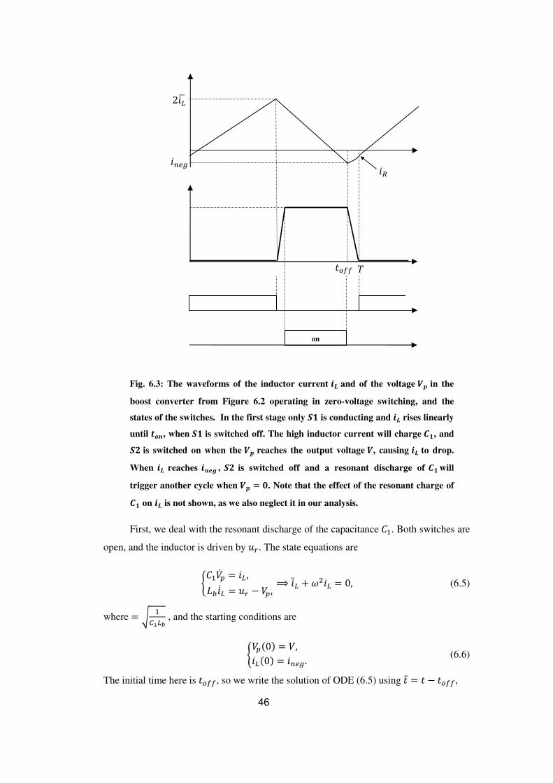
46

Fig. 6.3: The waveforms of the inductor current ®Ú and of the voltage G in the

boost converter from Figure 6.2 operating in zero-voltage switching, and the

states of the switches. In the first stage only s� is conducting and ®Ú rises linearly

until ×ØÙ, when s� is switched off. The high inductor current will charge Y�, and st is switched on when the G reaches the output voltage G, causing ®Ú to drop.

When ®Ú reaches ®Ùæä , st is switched off and a resonant discharge of Y� will

trigger another cycle when G = �. Note that the effect of the resonant charge of

Y� on ®Ú is not shown, as we also neglect it in our analysis.

First, we deal with the resonant discharge of the capacitance �.. Both switches are

open, and the inductor is driven by pÉ. The state equations are

��.�l� = %L ,WÐUllL = pÉ − ��, 1 ⟹ Ul§L +c�%L = 0, (6.5)

where = � .�7LÑ , and the starting conditions are

��(0) = �,%L(0) = %�d.1 (6.6)

The initial time here is �wòò, so we write the solution of ODE (6.5) using � = � − �wòò,

\

2UlLÏ

2UlLÏ

�wòò

%�d

on

%þ

47

�%L = Î sin(c�) + cos(c�),�� = pÉ −cWÐÎcos(c�) + cWÐ sin(c�).1 Applying the initial conditions (6.6) to the above solution we get

Î = (pÉ − �)v�.WÐ , = %�d, hence,

��%L = (pÉ − �)v�.WÐ sin(c�) + %�d cos(c�),�� = pÉ − (pÉ − �) cos(c�) + vWÐ�. %�d sin(c�).

1 (6.7)

(6.8)

The duration of the resonant discharge Δ�þ = \ − �wòò can be found from (6.8), by

solving for �� = 0. Through some algebraic calculations, denoting À�d = �LÑ�7 %�d� and

� = xÔgQxÔ-P��ýi��ýig Q�xÔ-P-g��ýig P(xÔQ-)g we obtain

Δ�þ = 1c cosQ.(�). (6.9)

The inductor current at the end of the resonant discharge, %þ, (see Figure 6.3) can be

found by substituting (6.9) for � in (6.7), obtaining

%þ = (pÉ − �)v�.WÐ �1 − �� + %�d�. (6.10)

Next, we find the duration of the descending part of the inductor current Δ�wòò = �wòò −�w using a linear relation with a slope

xÔQ-LÑ , hence,

Δ�wòò = WÐpÉ − � ~%�d − %þ − pÉWÐ �w�. (6.11)

Now, the average inductor current UlLÏ can be expressed as

UlLÏ = $ %L(�)'�Å) \ = �w + �wòò + �þ�w + Δ�wòò + Δ�þ, (6.12)

where �w is the charge flowing through the inductor until �w, �wòò is the charge

flowing from �w to �wòò and �þ is the charge flowing from �wòò to \.

48

�w can easily be calculated by integrating the rising inductor current:

�w = 5 ~pÉ�WÐ + %þ�'� = pÉ�w�2WÐ + %þ�w(Ò�) . (6.13)

By integrating the falling inductor current and substituting (6.11) we obtain:

�wòò = 5 ~pÉ − �WÐ � + pÉ�wWÐ + %þ�'��(Òôô)

= 12(pÉ − �) ¶WÐ %�d� − %þ�� − 2%þpÉ�w − pÉ��w�WÐ ·. (6.14)

Likewise, �þ is obtained by integrating (6.7) and substituting (6.9):

�þ = 5 �(pÉ − �)v�.WÐ sin(c�) + %�d cos(c�)��(�) '�

= (pÉ − �)�.(1 − �) + %�d��.WÐ(1 − ��).

(6.15)

Substituting the charges from (6.13-6.15), Δ�wòò from (6.11) and Δ�þ from (6.9) into

(6.12), we obtain after some algebraic manipulation:

UlLÏ= � �xÔ(Ò�g�LÑ + %þ�w� − LÑ� %�d� − %þ�� − (pÉ − �)��.(1 − �) − (pÉ − �)%�d��.WÐ(1 − ��)

��w − WÐ %�d − %þ� − (pÉ − �)��.WÐ cosQ.(�) . We substitute the above expression in (6.1), and solve the resulting equation to obtain

�w = �w2 − WÐ%þpÉ +v´�w2 − WÐ%þpÉ µ� − WÐpÉ� 4(�w), (6.16)

where

4(�w) = pÉ %�d − %þ��w − 2(pÉ − �)��.(1 − �) − WÐ %�d� − %þ��+ (pÉ − �)��.WÐ ~pÉWÐ �w cosQ.(�) − 2%�d�1 − ��.

The sign before the square root in (6.16) is positive, as at the limit �. → 0, %�d →0, %þ → 0 we require �w = �w (as in the non ZVS case). In practice, the real-time

calculation of �w from (6.16) in order to control a PFC is a demanding task. A linear

approximation of �w in the form

49

�w ≈ &(pÉ) + �(pÉ)�w, where &(pÉ) and �(pÉ) are pre-calculated coefficients, can be used to achieve very good

results. When comparing the approximated �w with the exact values of (6.16) in the

range 0.4μs − 4μs, we obtain an RMS error of 0.42ns and a maximal error of 2.3ns. In

addition, a discretization error should be taken into account as the look-up table

containing the coefficients is limited in size.

Operating Condition

The proper operation of the zero-voltage switching algorithm depends on the

negative inductor current which depletes the capacitance �. and drives �� to zero. In

order to obtain the conditions required for the above, we verify that the time Δ�þ from

(6.9) exists and is finite. We recall the argument of the arc-cosine in (6.9),

� = pÉ� − pÉ� + À�d�À�d� − 2pÉ� + ��À�d� + (pÉ − �)� .

First, the expression inside the square root must be non-negative, hence

À�d� ≥ �(2pÉ − �). (6.17)

Now we search for the minimal value of À�d that satisfies −1 O � O 1, the domain of

the arc-cosine (recall that À�d is proportional to %�d. We want to minimize the required

negative current since it causes conduction losses, therefore the higher values of À�d are

less significant). Since À�d, �, pÉ ∈ ℝP, we examine (6.17) under two cases:

1) pÉ O -� :

The inequality (6.17) is always true, and the minimal À�d which satisfies it is

À�d = 0. In this case, � = xÔxÔQ- satisfies −1 O � O 0, and no additional condition

is required.

2) pÉ > -� :

In this case time the inequality (6.17) becomes the operating condition that ensures

that �� falls to 0�. The minimal À�d is À�d� = �(2pÉ − �), thus � = xÔQ-xÔ which

satisfies −1 O � O 1 as required.

For example, for � = 400V, pÉ(ADE) = 340Vwe get (from case 2) À�d(ABC) ≈ 335V.

Using WÐ = 60μHand �. = 1.5nF, we obtain %�d(ADE) = −1.675A .

50

6.3. Simulation results of a ZVS PFC

The performance of the zero-voltage switching circuit from Figure 6.2 as part of

the PFC presented in the previous chapter has been examined in MATLAB simulations

using the SimPowerSystems toolbox. The parameters of the VIC are the same as in the

previous chapter. The parameters of the VIC charge controller (shown in Figure 3.5) are }� = 2 × 10Q.�, &� = 40ms, the initial value of the integrator is −0.075μs and the cut-

off frequency of the LPF is 20Hz ( o(n) = ..Pr] where & = 8ms). The parameters of the

PFC circuit (shown in Figures 5.1 and 6.2) are �HIJ = 400V,K = 320Ω (hence, the

power is 500W), WÐ = 60μH , �� = 100nF and �. = 1.5nF . The grid voltage is the

same as in the previous chapter. We have chosen %�d proportional to the voltage pÉ,

with a proportion constant }�d = −5mΩQ., which corresponds to a maximal %�d =−1.675A for the maximal pÉ (as calculated in the end of the previous section). The

results are shown in Figure 6.4.

The calculated total harmonic distortion (THD) of the input current %d (in the

range up to 4KHz) is about 9.2%. The low frequency voltage ripple seen in Figure 6.4(c)

is 2.08V peak-to-peak. A significantly lower ripple can be achieved by using the

integrating sliding function demonstrated in Chapter 5.4. Since �w , as calculated by

equation (6.16), has a component that divides by pÉ, it tends to infinity when pÉ → 0V.

Therefore, the adjusted �w must be limited by a saturation value, that we choose to be �w(ADE) = 50μs (no optimization was performed on this value). The higher THD than

that of the non-ZVS circuit and the small deviations from a sinusoidal waveform seen in

the zero-crossings of the current in Figure 6.4(a) are a result of the inability to accurately

reconstruct the desired sinusoidal average input current in low pÉ (near the zero-

crossings) due to the asymptote of �w . A better THD may be attainable if a tighter

(higher, and not proportional to pÉ) %�d is used, and if the capacitance �. is reduced (by

disconnecting any parallel capacitor) when pÉ is low. Some PFC methods can be

adjusted to mitigate this problem, such as a Frequency Clamped Critical conduction

Mode (FCCrM) [32], but this is not covered in this thesis.

51

Fig. 6.4: Simulation results for a zero-voltage switching PFC using a VIC. Three

grid cycles are shown in steady state operation. All the signals shown, except for

the last (d), are filtered via a low-pass filter with a cut-off frequency of 1KHz, to

eliminate the ripple noise of the boost converter. (a) the converter input current ®ä; (b) the VIC input current ®; (c) the voltage error Gïðñ − G; (d) the VIC inner

capacitor voltage Gs, used as a measure of F.

The power-up process of the converter is shown in Figure 6.5. A single episode of

in-rush current occurs during the first 5 microseconds. In contrast with the non-zero-

voltage switching circuit, there are no secondary in-rush episodes. That is since the

adjusted �w is greater than the unadjusted �w at the beginning of each semi-cycle,

which causes a greater inductor current that in turn causes a greater current to charge the

VIC (compare Figure 6.5(b) and Figure 5.5(b)). As in the non-ZVS version, this circuit

does not exhibit PFC properties during the power-up stage since �w is not constant.

0.5 0.51 0.52 0.53 0.54 0.55 0.56-4

-2

0

2

4

time [sec]

i g [A

]

0.5 0.51 0.52 0.53 0.54 0.55 0.56

-1

0

1

time [sec]

i [A

]

0.5 0.51 0.52 0.53 0.54 0.55 0.56

0

1

2

time [sec]

Verr

or [

V]

0.5 0.51 0.52 0.53 0.54 0.55 0.56100

200

300

400

time [sec]

VS [V

](a)

(b)

(c)

(d)

52

Fig. 6.5: Simulation results for the power-up phase of the ZVS PFC using a VIC.

Only the first semi-cycle of the grid voltage is shown here. (a) the converter input

current ®ä; (b) the VIC input current ®; (c) the output voltage G; (d) the VIC

inner capacitor voltage Gs, used as a measure of F.

Figure 6.6 shows the stability of the output voltage during an increase and a decrease of

the output power. Upon reaching stability, as in Figure 6.4, the load power changes at

0.515 seconds from 250W to 500W and back to 250W at 0.545 seconds. The input

current during the semi-cycle in which the power change occurs does not retain a

sinusoidal form, since �w must be changed in order to keep the VIC within the flat

operating region, as described in the previous chapter.

0 0.001 0.002 0.003 0.004 0.005 0.006 0.007 0.008 0.009 0.01

0

5

10

15

time [sec]

i g [

A]

0 0.001 0.002 0.003 0.004 0.005 0.006 0.007 0.008 0.009 0.01

-1

0

1

2

3

time [sec]

i [A

]

0 0.001 0.002 0.003 0.004 0.005 0.006 0.007 0.008 0.009 0.010

200

400

time [sec]

V [

V]

0 0.001 0.002 0.003 0.004 0.005 0.006 0.007 0.008 0.009 0.010

200

400

time [sec]

VS [

V]

(a)

(b)

(c)

(d)

53

Fig. 6.6: Simulation results for an output power changes in a ZVS PFC using a

VIC. At time 0.515sec the power changes from 250W to 500W, and at time

0.545sec it changes back to 250W. Three grid cycles are shown. The signals (a),

(c), (d) are filtered via a low-pass filter with a cut-off frequency of 1KHz, to

eliminate the ripple noise of the boost converter. (a) the converter input current ®ä; (b) the converter output current ®Ø�× ; (c) the VIC input current ®; (d) the

voltage error Gåæç − G; (e) the VIC inner capacitor voltage Gs, used as a measure

of F.

6.4. ZVS implementation of the VIC

In order to be a proper replacement for a large capacitor and not significantly

reduce the overall efficiency of the circuit using it, any implementation of the VIC must

be extremely efficient, and not cause power losses that are much greater than the losses

in the ESR of an equivalent electrolytic capacitor. Since the VIC must operate in a very

high switching frequency (several hundred kHz), the switching losses of the

0.5 0.51 0.52 0.53 0.54 0.55 0.56-4-2024

time [sec]i g

[A

]

0.5 0.51 0.52 0.53 0.54 0.55 0.560

0.5

1

1.5

time [sec]

i ou

t [A

]

0.5 0.51 0.52 0.53 0.54 0.55 0.56

-101

time [sec]

i [A

]

0.5 0.51 0.52 0.53 0.54 0.55 0.56

0

1

2

time [sec]

Ve

rro

r [V

]

0.5 0.51 0.52 0.53 0.54 0.55 0.56100

200

300

400

time [sec]

VS

[V

]

(a)

(b)

(c)

(d)

(e)

implementation presented in Chapter 4

calculations from the beginning of this chapter,

each switching, one MOSFET is turned on (which also discharges its parallel capacitance �w]]) and the other is turned off. We assume that the parallel diodes do not conduc

no reverse recovery current contributes to the power loss. For ease of calc

roughly approximate �]voltage on each MOSFET is the same

(two switchings of each MOSFET)

MOSFET chosen in Section 6.1

4]� =where U = 1.8A (see Chapter 5) is the average of the absolute valu

the switching time (obtained from simulation)

�É = 17nsec is the current rise time [

(similarly to (6.2)). Since the switching frequency is

estimated switching power loss would be

Fig 6.7: A realization of a

capacitance of the switches,

voltage on the lower switch.

In order to reduce the switching losses, we need t

was done for the PFC stage.

switches, ��, shown in Figure 6.7.

can be implemented, if we can con

control the average inductor current

operating in critical mode is shown in Figure 6.8. Note

%

_

C

+

�

54

implementation presented in Chapter 4 are expected to be high. Following our

the beginning of this chapter, we can estimate the switching losses

each switching, one MOSFET is turned on (which also discharges its parallel capacitance

) and the other is turned off. We assume that the parallel diodes do not conduc

no reverse recovery current contributes to the power loss. For ease of calc

to be 200V and neglect the voltage drop on the inductor

voltage on each MOSFET is the same. Hence, the energy loss in each

(two switchings of each MOSFET), under the condition given in Section 5.3 and the

MOSFET chosen in Section 6.1 is

�w]]�]� T U�] �Éx T �ò T �òx T �É� 39.8μJ, (see Chapter 5) is the average of the absolute value of the VIC current

the switching time (obtained from simulation), �Éx, �ò are the same as in Section 6.1,

is the current rise time [21] and �òx 18nsec is the voltage fall time

Since the switching frequency is �] 246kHz (see Figure 4.6), the

switching power loss would be �]� 4]��] Ê 9.8W.

realization of a VIC, showing the parallel parasitic

capacitance of the switches, Y (compare Figure 3.4). � denotes the

voltage on the lower switch.

In order to reduce the switching losses, we need to implement a ZVS algorithm, as

for the PFC stage. In ZVS, we make use of the parasitic capacitance of the

, shown in Figure 6.7. A similar technique to that described in Section 6.2

can be implemented, if we can control the VIC in a critical mode, which

inductor current %] of the VIC. An average model of the VIC

operating in critical mode is shown in Figure 6.8. Note that it is different than the

%�

/M

/

í

�� W

�� R �R %R

�.

��

be high. Following our

n estimate the switching losses. On

each switching, one MOSFET is turned on (which also discharges its parallel capacitance

) and the other is turned off. We assume that the parallel diodes do not conduct, so

no reverse recovery current contributes to the power loss. For ease of calculation, we

n the inductor, so the

in each switching cycle

, under the condition given in Section 5.3 and the

e of the VIC current at

are the same as in Section 6.1,

is the voltage fall time

(see Figure 4.6), the

parallel parasitic

denotes the

o implement a ZVS algorithm, as

In ZVS, we make use of the parasitic capacitance of the

A similar technique to that described in Section 6.2

critical mode, which allows us to

An average model of the VIC

it is different than the

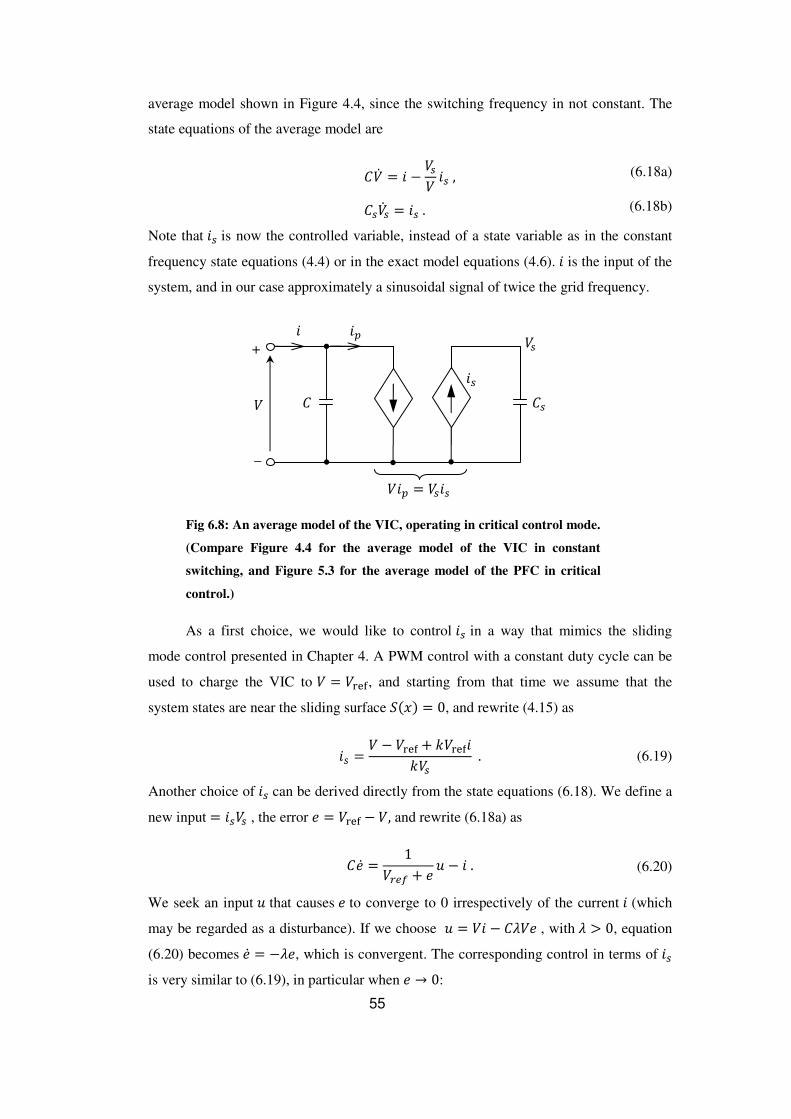
55

average model shown in Figure 4.4, since the switching frequency in not constant. The

state equations of the average model are

��l % −

�]�%],

�]�l] %].

(6.18a)

(6.18b)

Note that %] is now the controlled variable, instead of a state variable as in the constant

frequency state equations (4.4) or in the exact model equations (4.6). % is the input of the

system, and in our case approximately a sinusoidal signal of twice the grid frequency.

Fig 6.8: An average model of the VIC, operating in critical control mode.

(Compare Figure 4.4 for the average model of the VIC in constant

switching, and Figure 5.3 for the average model of the PFC in critical

control.)

As a first choice, we would like to control %] in a way that mimics the sliding

mode control presented in Chapter 4. A PWM control with a constant duty cycle can be

used to charge the VIC to � �HIJ, and starting from that time we assume that the

system states are near the sliding surface �(�) = 0, and rewrite (4.15) as

%] � � �HIJ T ��HIJ%��] . (6.19)

Another choice of %] can be derived directly from the state equations (6.18). We define a

new input %]�] , the error � �HIJ � �, and rewrite (6.18a) as

��l 1�É�ò T � p � %. (6.20)

We seek an input p that causes � to converge to 0 irrespectively of the current % (which

may be regarded as a disturbance). If we choose p �% � �� , with � > 0, equation

(6.20) becomes �l ��, which is convergent. The corresponding control in terms of %] is very similar to (6.19), in particular when � → 0:

%]

%

_

%�

�] �

�] +

�

�%� �]%]

56

%] � � �HIJ T ��%��] . (6.21)

Substituting (6.21) into the state equations (6.18b), we obtain a set of differential

equations

��l � �� ,�]�l] ��% − ��] ,

(6.22a)

(6.22b)

We observe that the first equation (6.22a) is decoupled from the second (independent of

�]), and stable as designed by our choice of p. The second equation (6.22b) with � 0

becomes

12� ''� (�]�) = �%, which means that the derivative of the stored energy equals the flow of the power into

the VIC.

The implementation of the critical conduction mode controller of the VIC using U] (the average value of %] over one switching cycle), determined by either (6.19) or (6.21),

requires us to take a different approach than used in Section 5.2 for the PFC control,

since U] may take either positive or negative values. Hence, we control either the duration

of the rising current if U] > 0, or the duration of the falling current if U] ? 0 (denoted �w

in both cases). Typical waveforms of %], í and the state of the switches are shown in

Figure 6.9. From simple calculations, we get:

�w 2W� − �] U]forU] ≥ 0,�w � 2W�] U]forU] < 0.

(6.23a)

(6.23b)

We explain the positive U] switching cycle, which is symmetrical to the negative case:

when / 1 the current %] rises for a duration �w which is calculated from (6.23). �.is

then turned off, and the voltage í drops to zero in resonant conditions driven by a

positively high %]. When í 0, �� is switched on (in ZVS conditions) and %] starts to

drop. When %] reaches zero, the desired average current U] is calculated using (6.19) or

(6.21), the controller decides if the next switching cycle is a positive "triangle" or a

negative one, and chooses �w accordingly. If the next cycle is a negative one, it starts at

that time with a falling %], otherwise �� is switched off and the resonant charge of its

57

capacitance causes í to reach �, and another switching cycle starts. We do not correct

�w based on the duration of the resonant stages, as we do in the ZVS control of the PFC

(see Chapter 6.2), since the errors that are caused by this inaccuracy can be adequately

corrected as shown later in this chapter.

Fig. 6.9: The waveforms of the inductor current ®" and the voltage � in a

VIC controlled in a critical conduction mode, showing the state of the

switches. ½ denotes the end of each switching cycle, and the start of a

new counting towards ×ØÙ. The first two switching cycles are positive,

while the third is a negative one. Note that ×ØÙ determines the duration of

the "on" state of s� for a positive triangle, and of st for a negative one.

Simulation results of the ZVS PFC that was introduced in Chapter 6.3, with a ZVS

VIC operating in critical conduction mode, are shown in Figure 6.10. The critical

conduction mode controller uses equation (6.21) to determine U], with � = 0.004. All the

conditions of the simulation are as in Chapter 6.3, and the capacitors �� 0.5nF. The

calculated switching loss is less than 0.1W (using the method explained in the beginning

of this section), and the conduction loss is about 1.25W. Switching losses occur when the

current %] during the resonant stage is not high enough for driving í to 0 (or to �), which

%]

%L

í

��

� �

�w

�\

�

�

� ��

�.

�1��

�2

on on

on

0

0

0

0

on

�w �w \ � �

\

on

58

forces a non-zero-voltage switching. The simulated RMS of the error in � (low-pass

filtered at 1kHz) is 0.52V, and the peak-to-peak ripple is 1.67V.

Fig. 6.10: Simulation results for a PFC using a ZVS VIC with the critical

conduction mode controller (6.21). Three grid cycles are shown in steady state

operation. The signals (except Gs) pass through an LPF with cut-off frequency of

1kHz. The low frequency ripple is 1.67V peak-to-peak. The meaning of all the

signals is as in Figure 5.4.

We now consider a model that takes into account the imperfections in generating

the current %] , due to the complexity of generating the exact positive and negative

triangles and the presence of transients. We examine a third controller, based on the

integral sliding function (5.6), including the noise #:

%] = ��] ´% − �2$c� − �c�5 �(�)'�() µ + #, (6.24)

0.12 0.13 0.14 0.15 0.16 0.17 0.18-4

-2

0

2

4

time [sec]

i g [

A]

0.12 0.13 0.14 0.15 0.16 0.17 0.18

-1

0

1

time [sec]

i [A

]

0.12 0.13 0.14 0.15 0.16 0.17 0.18

-1

-0.5

0

0.5

1

time [sec]

Verr

or [

V]

0.12 0.13 0.14 0.15 0.16 0.17 0.18100

200

300

400

time [sec]

Vs [

V]

(a)

(b)

(c)

(d)

59

where $ and c are control constants (which relate to �, �ì from (5.6)). Substituting

(6.24) in (6.18), we obtain the closed loop system

��l = �2$c� + �c�5 �(�)'�() + �]� #,

�]�l] = ��] ´% − �2$c� − �c�5 �(�)'�() µ + #,

or equivalently,

�l + 2$c� + c�5 �(�)'�() = − �]�� #,

� ''� (�]�) = 2� ´% − �2$c� − �c�5 �(�)'�() µ + �]#.

(6.25a)

(6.25b)

If we denote c = − -�- #, then (6.25a) becomes �§ + 2$c�l + c�� = cl , so the transfer

function from c to � is

%(n) = nn� + 2$cn + c�. (6.26)

For large enough |n| we have %(n) ≈ 1/n, so that the right asymptote of % (see Figure

6.11) is always the same, regardless of c and $. In theory, the larger we choose c

(while keeping, for example, $ = 1), the better. In practice, for very large c, the system

becomes unstable, because of modeling inaccuracies. Figure 6.12 shows the simulated

results of the controller (6.24), with constants $ = 7.8125,c = 10000 HD&' . Similarly to

the results of the controller from Chapter 5.4, the obtained ripple on � is reduced

significantly to about 14mV RMS.

Fig. 6.11: Asymptotic gain Bode plot of the transfer function (6.26), showing

that when using the controller from (6.24), the noise is low in frequencies

both higher and lower than (Ù.

c

c gain

12$c

1

20dB dec⁄ −20dB dec⁄

60

Fig. 6.12: Simulation results for a PFC boost converter using a VIC with the

improved integral critical mode controller (6.24). Three grid cycles are shown in

steady state operation. The signals (except Gs) pass through an LPF with cut-off

frequency of 1kHz. This filter is insufficient to smooth he signal GæååØå = Gïðñ − G

in this scale, yet it is evident that the low frequency ripple is in order of 50mV.

The meaning of all the signals is as in Figure 5.4.

0.12 0.13 0.14 0.15 0.16 0.17 0.18-4

-2

0

2

4

time [sec]i g

[A

]

0.12 0.13 0.14 0.15 0.16 0.17 0.18

-1

0

1

time [sec]

i [A

]

0.12 0.13 0.14 0.15 0.16 0.17 0.18-0.1

-0.05

0

0.05

0.1

time [sec]

Verr

or [

V]

0.12 0.13 0.14 0.15 0.16 0.17 0.18100

200

300

400

time [sec]

Vs [

V]

(a)

(b)

(c)

(d)

61

7. Conclusion

In this thesis we have introduced the VIC, an electronic circuit that replaces a large

filter capacitor. Realizations of the VIC using a bidirectional DC/DC converter with a

sliding mode or a critical mode control have been proposed, as well as a zero-voltage-

switching realization. An application of the VIC as a component in the boost converter of

a PFC was studied and simulated, using a capacitor 1000 times smaller than an

equivalent filter capacitor required to achieve the same output voltage ripple.

The use of much smaller capacitors instead of electrolytic capacitors contributes

to higher reliability and smaller devices. Therefore, the VIC can replace the input or

output capacitors in various power converters, where there is a significant low frequency

current flowing through the capacitor. Typical applications are in PFCs and in single

phase inverters.

As a continuation of this work, we are planning to build a working prototype of

the VIC. A possible new application as the energy storage device in a synchronverter

[49] is being explored. In this application, the VIC will be used in an inverter to emulate

the inertia of a synchronous generator. In such applications, when a much large energy

storage is needed, a VIC using batteries (as will be first implemented in the

synchronverter now being built in our lab) or supercapacitors may prove more useful.

Several improvements can be made to our zero-voltage switching controllers:

when the needed current U] in the critical mode controlled VIC is very small (see Chapter

6.4), the controller creates alternating positive and negative triangles in the %] waveforms

(see Figure 6.9) that cause unnecessary conduction losses. Opening both switches when %] hits zero, and introducing a delay between consecutive triangles may reduce those

losses. The ZVS control of the PFC stage may also include a closed loop controller that

observes and corrects the current in the inductor W], instead of the complex open loop

correction of �w explained in Chapter 6.2.

Other topologies of the VIC may be useful in some applications. For example,

when the power requirements from the VIC are high and the reliability of the product is

important, a VIC using a very large film capacitor would be very expensive. An

equivalent topology where the capacitor inside the VIC works at a higher v oltage than

the input may be more economic, as film capacitors can withstand high voltages, and the

capacitance needed would be much lower (since the energy in the capacitor depends on

the square of the voltage across it).

62

Fig. 7.1: F-G characteristics of a virtual "big" capacitor (compare with Figure 2.1)

Similar to the VIC, which has 3 terminals and requires an external controller, a

virtual "big" capacitor, which has the � − � plot shown in Figure 7.1, can be

constructed. Such a device has only 2 terminals, similar to a regular capacitor, and the

voltage across it can be used to determine its charge. This adaptation (which can be

easily implemented by changing �HIJ as a function of �]) may ease the integration of the

VIC in various systems. Another idea based on the VIC is a virtual infinite inductor. This

device is defined as having a constant current over a range of magnetic fluxes, and may

be useful as a current regulator in applications such laser diodes and precise magnetic

instruments.

Q

V

maxQ minQ

refV

63

8. Bibliography

[1] AN-42047: Power Factor Correction (PFC) basics, Fairchild Semiconductor Co.

San-Jose, CA, 2004.

[2] W. Andreycak, “Zero voltage switching resonant power conversion”, UNITRODE

Power Supply Design Seminar SEM-700, 1990.

[3] J. A. Bassett, "New, zero voltage switching, high frequency boost converter

topology for power factor correction," in Proc. of INTELEC, The Hague,

Netherlands, Oct. 1995.

[4] L. O. Chua, Introduction to Nonlinear Network Theory. New York: McGraw-Hill,

1967.

[5] L. O. Chua, "Synthesis of new nonlinear network elements," in Proc. of IEEE, vol.

56, no. 8, pp. 1325-1340, 1968.

[6] D. Cortez, J. Alvarez and J. Alvarez, "Robust sliding mode control for the boost

converter," in Proc. of CIEP, Guadalajara, Mexico, Oct. 2002.

[7] M. Di Ventra, Y. V. Pershin and L. O. Chua, "Circuit elements with memory:

memristors, memcapacitors and meminductors," in Proc. of IEEE, vol. 97, no. 10,

Oct. 2009.

[8] C. Edwards and S. K. Spurgeon, Sliding Mode Control: Theory and Applications.

London, U.K.: Taylor & Francis, 1998.

[9] G. Escobar and H. Sira-Ramirez, "A passivity based-sliding mode control approach

for the regulation of power factor precompensators," in Proc. of IEEE conf. on

Decision and Control, Tampa, FL, Dec. 1998.

[10] L. Fridman, J. Moreno, R. Iriate (eds.), Sliding modes after the first decade of the

21st century. Berlin: Springer, 2011.

[11] E. Garcia-Canseco, R. Griño, R. Ortega, M. Salichs and A. M. Stankovic, "Power

factor compensation of electrical circuits," IEEE Control Systems, vol. 27, no. 2, pp.

44-59, Apr. 2007.

[12] A. Gee, F. V. P. Robinson, and R. W. Dunn, "Sliding-mode control, dynamic

assessment and practical implementation of a bidirectional buck/boost DC-to-DC

converter," in Proc. of EPE, Ohrid, Macedonia, 2011.

[13] M. Gotfryd, "Limits in boost power factor corrector operating in border-line mode,"

IEEE Trans. Power Electron., vol. 18, no. 6, pp.1330-1335, Nov. 2003.

64

[14] D. Graovac, M. Pürschel and A. Kiep, "MOSFET power losses calculation using the

data-sheet parameters", Infineon Tech. AG, Neubiberg, Germany, Jul. 2006.

[15] S. Guo, X. Lin-Shi, B. Allard, Y. Gao and Y. Ruan, "Digital sliding-mode controller

for high-frequency DC/DC SMPS", IEEE Trans. Power Electron., vol. 25, no. 5, pp.

1120-1123, May 2010.

[16] Harmonic current emissions – Guidelines to the standard EN 61000-3-2, ESPMA,

Wellingborough, UK, Nov. 2010.

[17] C. P. Henze, H. C. Martin and D. W. Parsley, "Zero-voltage switching in high

frequency power converters using pulse width modulation," in Proc. of APEC, New

Orleans, LA, Feb. 1988.

[18] A. Hijazi, M. Di Loreto, E. Bideaux, P. Venet, G. Clerc and G. Rojat, "Sliding mode

control of boost converter: application to energy storage system via

supercapacitors," in Proc. of EPE, Barcelona, Spain, 2009.

[19] G. Hua, C.-Sh. Liu, Y. Jiang and F. C. Y. Lee, "Novel zero-voltage-transition PWM

converters," IEEE Trans. Power Electron., vol. 9, no. 2, pp. 213-219, Mar. 1994.

[20] IEC Technical Report 62380:2004(E): Reliability data handbook – universal model

for reliability prediction of electronic components, PCBs and equipment, IEC,

Geneva, Switzerland, Aug. 2008.

[21] IPP60R250CP Data Sheet, Rev. 2.1, Infineon Tech. AG, München, Germany, Jan.

2012.

[22] IDH10G65C5 Data Sheet, Rev. 2.1, Infineon Tech. AG, München, Germany, Sep.

2012.

[23] J. G. Kassakian, M. F. Schlecht and G. C. Verghese, Principles of Power

Electronics. Reading, MA: Addison-Wesley, 1992.

[24] J.-S. Lai and D. Chen, "Design consideration for power factor correction boost

converter operating at the boundary of continuous conduction mode and

discontinuous conduction mode," in Proc. of APEC, San Diego, CA, Mar. 1993.

[25] A. Levant, "Sliding order and sliding accuracy in sliding mode control," Int. J.

Control, vol. 58, pp. 1247-1263 ,1993.

[26] R. L. Lin and F. C. Y. Lee, "Novel zero-current-switching-zero-voltage-switching

converters," in Proc. of PESC, Baveno, Italy, June 1996.

[27] J. Liu and N. Henze, "Reliability consideration for low-power grid-tied inverter for

photovoltaic application," in Proc. of EU PVSEC, Hamburg, Germany, 2009.

[28] K.-H. Liu and F. C. Y. Lee, "Zero-voltage switching technique in DC/DC

Converters," IEEE Trans. Power Electrons., vol. 5, no. 3, pp. 293-304, Jul. 1990.

65

[29] J. M. Manley and H. E. Rowe, "Some general properties of nonlinear elements –

Part I: general energy relations," in Proc. of IRE, vol. 44, no. 7, pp. 904-913, 1956.

[30] R. Naim, G. Weiss and S. Ben-Yaakov, "H∞ control applied to boost power

converters,", IEEE Trans. Power Electron., vol. 12, no. 4, pp. 677-683, 1997.

[31] R. Ortega, A. Loria, P. J. Nickolasson and H. Sira-Ramirez, Passivity-based Control

of Euler-Lagrange Systems. London, UK: Springer Verlag, 1998.

[32] Power Factor Correction (PFC) Handbook, Rev. 4, ON Semiconductor, Denver,

CO, Feb. 2011.

[33] M. H. Rashid, Power Electronics: Circuits, Devices, and Applications, 2nd ed.,

Englewood Cliffs, NJ: Prentice-Hall Inc., 1993, pg. 487-490.

[34] C. Rodriguez and G. A. J. Amaratunga, "Long-lifetime power inverter for

photovoltaic AC modules," IEEE Trans. Ind. Elect. vol. 55, no. 7, pp. 2593-2601,

Jul. 2008.

[35] H. E. Rowe, "Some general properties of nonlinear elements – Part II: small signal

theory," in Proc. of IRE, vol. 46, no. 5, pp. 850-860, 1958.

[36] H. Sira-Ramirez, "Sliding motions in bilinear switched networks," IEEE Trans.

Circuits and Systems, vol. 34, no. 8, pp. 919-933, 1987.

[37] G. Spiazzi, P. Mattavelli and L. Rossetto, "Sliding mode control of DC-DC

converters," in Proc. 4th Congresso Brasileiro de Elettronica de Potencia

(COBEP), Belo Horizonte, Spain, 1997.

[38] C. G. Steyn and J. D. Van Wyk, "Study and application of nonlinear turn-off

snubber for power electronic switches," IEEE Trans. Ind. Appl. vol. IA-22, no. 3,

May/Jun. 1986.

[39] W. A. Tabisz and F. C. Y. Lee, "Zero-voltage-switching multi-resonant technique –

a novel approach to improve performance of high frequency quasi-resonant

converters," in Proc. of PESC, Kyoto, Japan, Apr. 1988.

[40] S.-C. Tan, Y. M. Lai and C. K. Tse, "General design issues of sliding-mode

controllers in DC-DC converters," IEEE Trans. Ind. Electron., vol. 55, no. 3, pp.

1160-1173, Mar. 2008.

[41] S.-C. Tan, Y. M. Lai and C. K. Tse, "Implementation of pulse-width-modulation

based sliding mode controller for boost converters," IEEE Power Electron. Letters,

vol.3, no. 4, pp. 130-135, Dec. 2006.

[42] V. I. Utkin, "Sliding mode control," in Variable Structure Systems: From Principles

to Implementation, A. Sabanovic, L. Fridman and S. Spurgeon (eds.), Institute of

Electrical Engineers, 2004.

66

[43] V. I. Utkin and J. Shi, "Integral sliding mode in systems operating under uncertainty

conditions," in Proc. of CDC, Kobe, Japan, Dec. 1996.

[44] V. Vorperian, "Quasi-square-wave converters: topologies and analysis," IEEE

Trans. of Power Electron., vol. 3, no. 2, pp. 183-191, Apr. 1988.

[45] E. Walker, "Design review: a step-by-step approach to AC line-powered

converters," in TI Unitrode Design Seminar Series, 2005

[46] R.-J. Wai and L.-C. Shih, "Design of voltage tracking control for DC-DC boost

converter via total sliding-mode technique", IEEE Trans. Ind. Electron., vol. 58, no.

6, pp. 2502-2511, Jun. 2011.

[47] K. D. Young, V. I. Utkin and U. Özgüner, "A control engineer's guide to sliding

mode control," IEEE Trans. Control Systems Tech., vol. 7, no. 3, pp. 328-342, May

1999.

[48] X. Yuan and I. Barbi, "Analysis, designing and experimentation of a transformer-

assisted PWM zero-voltage switching pole inverter," IEEE Trans. of Power

Electron., vol. 15, no. 1, pp. 72-82, Jan. 2000.

[49] Q.-C. Zhong and G. Weiss, "Synchronverters: inverters that mimic synchronous

generators," IEEE Tran. Ind. Electron., vol. 85, no. 4, pp. 1259-1267, Apr. 2011.

67

תקציר

ליניארי בעל התכונה שעבור �כקבל לא) VIC(סופי וירטואלי �אנו מגדירי� קבל אי�

אנו מציעי� מימוש . נשאר קבוע � ההדקי� שלו מתח, הנמצא בתחו� מסוי� �מטע�

סליל ושני , תו� שימוש ברכיבי מיתוג, סופי הוירטואלי�חסר הפסדי� של הקבל האי�מקורב

ופי ס�הקבל האי�. אותו אנו מתארי�, המעגל מחייב אלגורית� בקרה מורכב. קבלי�

מקד� הספק תיקו�כגו� מעגל , פק ביישומי� רבי�הוירטואלי שימושי כקבל סינו� הס

)PFC( ,סופי �הקבל האי�, במימוש המוצע למרות השימוש בקבלי� קטני�. המוצג בתזה זו

, הוירטואלי יכול להחלי קבלי� גדולי� מאוד ביישומי� שאינ� דורשי� אגירת אנרגיה רבה

) PFC(מקד� הספק תיקו� של מעגלמדגימי� תוצאות סימולציה אנו . כגו� סינו� הספק

סופי �העושה שימוש בקבל אי�, )critical conduction mode( קריטיהעובד במשטר הולכה

ימימושומנתחי� מדגימי� אנו , כמו כ�. סינו� מתח המוצא של המעגלייצוב ווירטואלי עבור

סופי הוירטואלי ושל מעגל �של הקבל האי� )zero-voltage switching(אפס �מתחב�מיתוג

. תיקו� מקד� ההספק

68

אביב �אוניברסיטת תל ש איבי ואלדר פליישמ�"הפקולטה להנדסה ע

סליינר�ש זנדמ�"בית הספר לתארי� מתקדמי� ע

סופיי� וירטואליי��קבלי� אי�

בהנדסת חשמל ואלקטרוניקה " מוסמ� אוניברסיטה"חיבור זה הוגש כעבודת גמר לקראת התואר

על ידי

גיא יונה

העבודה נעשתה בבית הספר להנדסת חשמל

וויס' ורג'ג' בהנחיית פרופ

ג"שבט תשע

69

אביב �אוניברסיטת תל ש איבי ואלדר פליישמ�"הפקולטה להנדסה ע

סליינר�ש זנדמ�"עבית הספר לתארי� מתקדמי�

סופיי� וירטואליי��קבלי� אי�

בהנדסת חשמל ואלקטרוניקה " מוסמ� אוניברסיטה"חיבור זה הוגש כעבודת גמר לקראת התואר

על ידי

גיא יונה

ג"שבט תשע

guy yona - taurel006/vic_thesis.pdf · a thesis submitted toward the degree of ... mppt maximum...

Documents